multi-echelon reverse supply chain … · with specified returns using particle swarm optimization...

International Journal of InnovativeComputing, Information and Control ICIC International c©2012 ISSN 1349-4198Volume 8, Number 10(A), October 2012 pp. 6719–6731

MULTI-ECHELON REVERSE SUPPLY CHAIN NETWORK DESIGNWITH SPECIFIED RETURNS USING PARTICLE

SWARM OPTIMIZATION

Zhen-Hua Che1,∗, Tzu-An Chiang2 and Yu-Chun Kuo1

1Department of Industrial Engineering and ManagementNational Taipei University of Technology

No. 1, Sec. 3, Chung-hsiao E. Rd., Taipei 10608, Taiwan∗Corresponding author: [email protected]

2Department of Business AdministrationNational Taipei College of Business

No. 321, Sec. 1, Jinan Rd., Taipei 10051, [email protected]

Received January 2011; revised June 2011

Abstract. This paper focuses on the development of an optimization mathematicalmodel for a reverse supply chain network that contains forward and reverse logisticalplans in the multi-echelon system. In the reverse process, the defective products are re-turned to the original manufacture/supplier (specified returns) to be produced again. Thenext period covers the quantity of defective products for the present period, as well asthe demands for the new period. To solve the mathematical model efficiently, a particleswarm optimization (PSO) solution is proposed, called PSOsm. The PSOsm introducesthe saltation mechanism into the procedure of the original PSO to increase the searcharea, which prevents the solution being laid on the local solution. Finally, to illustratethe performance of the PSOsm, the original PSO and a genetic algorithm (GA) are em-ployed to find the solution for the proposed problem and the performance of both methodsis compared. The results show that the PSOsm provides a better solution.Keywords: Reverse supply chain, Specified returns, Particle swarm optimization, Ge-netic algorithm

1. Background and Related Works. Supply chain management has become an im-portant strategic process for the coordination of supply chain networks that increasea company’s competitiveness in the current business environment [1-7]. Sadjady andDavoudpour [8] stated that designing distribution networks – as one of the most impor-tant strategic issues in supply chain management – has become the focus of researchattention in recent years and Das and Chowdhury [9] pointed out consideration of reverselogistics as a significant part of overall business process has been gaining importanceacross the entire global market. Dowlatshahi [10] also pointed out that reverse logisticsis an important concept for logistics and supply chain management and that efficientreverse logistics management can increase the competitiveness of an enterprise and pre-vent expulsion from the market, especially when facing intense competition and low profitmargins.

Shih [11] suggested that the reverse logistics system is an essential part of businessoperations when the recovery rates and service coverage are broadened, in the future.Desai and Mital [12] suggested that enterprises should work on the reuse, reworking,recycling, and reutilization of products at the end of the product life cycle. Hu et al.[13] stated that reverse logistics involves the complex logistics of management procedures,

6719

6720 Z.-H. CHE, T.-A. CHIANG AND Y.-C. KUO

which includes planning, management and control of the discarded logistics generated byrework and the disposal of discarded products. Imre [14] proposed that reverse logisticsinvolves the recycling of materials that could be reused in the market. If reverse logisticsis economically viable, it could protect the environment and reduce resources waste, whichmight provide a new use for recycled products. According to one conservative estimate,reverse logistics may account for 4% of total logistical costs [15]. According to Daugherty’sstudy, the average reverse logistics may account for 9.49% of total logistical costs [16].Therefore, reverse logistics may become critical to the success of many enterprises.The traditional supply chain focuses only on logistics, which is the sale of products,

and has neglected possible damage that may occur after the products are sold, seeminglyignoring the unavoidable fact that some non-conforming products would be generated inthe production and transportation processes. Therefore, when customers discover thatthey have bought non-conforming products, they would surely want the original manu-facturer to take responsibility. The distribution problem of returning the non-conformingproducts to the original manufacturers needs to be taken into account. The network forthis specific return supply chain is shown in Figure 1.To the best of our knowledge, no mathematical model for supply chain planning prob-

lems in multi-echelon networks that considers specified returns has been presented, eventhough it represents a better operational practice. Therefore, this paper emphasizes thedevelopment of an optimization mathematical model to deal with the problem of a reversesupply chain with specified returns.

Figure 1. Network concept for reverse logistics with specified returns

MULTI-ECHELON REVERSE SUPPLY CHAIN NETWORK DESIGN 6721

Gen and Cheng [17] indicated that a multi-stage stage logistical problem can be treatedas the combination of a multiple-choice Knapsack problem and a capacitated location-allocation problem as a NP-hard problem. In this study, every copartner has constrainedinformation about not only capacity, but also rate of loss, rate of defective items and thespecified returns. Hence, the task is more difficult for this problem.

Some previous research has proposed heuristic approaches for the design of forward/rev-erse supply chain networks, which can find near optimal solutions very quickly [18-21].PSO has been proven as an effective and simple optimization algorithm [22]. Cui etal. [23] and Yu et al. [24] stated that PSO is a practicable method for the solution ofoptimization problems. Some studies [25-30] have also pointed out that PSO is a usefulheuristic approach that can easily produce acceptable solutions to complex problems.Azadeh et al. [31] proposed a particle swarm optimization (PSO) algorithm to determinethe optimal inspection policy in serial multi-stage processes. Che and Cui [32] proposed aPSO method for Unbalanced Supply Chain Design. Sinha et al. [33], Mahnam et al. [34],Yang and Lin [35] and Che [30] successfully applied the PSO to the solution of supplychain planning problems. However, the above studies did not deal with a multi-echelonsupply chain planning problem that considers specified returns. Another purpose of thisstudy, therefore, is to present a modified PSO method (PSOsm) for the solution of theoptimization mathematical model developed for reverse supply chain network design withspecified returns.

The remainder of this paper is organized as follows. Section 2 develops an optimizationmathematical model to deal with the problem. The proposed heuristic solution model,PSOsm, is presented for the solution of the mathematical model in Section 3. Section 4presents detailed applications of the proposed method. Section 5 compares the experimen-tal results for PSOsm, PSO and GA, to determine the performance of PSOsm. Section 6presents the conclusions.

2. Optimization Mathematical Model for Supply Chain Network Design. Costand quality are the criteria used for the design of the supply chain network in this study.Before the data is used, a T -transfer technique is employed to transfer the original valuesof these two criteria to the standard T scores and to further integrate these scores. TheT -transfer formula for the original value, C, is Cs = (C−mean(C))/(Stand(C)/10)+50,where mean(C) is the mean value of C and Stand(C) is the standard deviation of C.

The notations used in the optimization optimizing mathematical model are as follows:

i Supply chain echelons, i = 1, 2, 3, . . ., I

p Production periods, t = 1, 2, 3, . . ., T

I Total number of echelons in the supply chain

P Total periods of production

j Copartner index

k Copartner index of the specified return

Ji Total number of copartners at echelon i

Ki Total number of copartners for the specified return at echelon i

INC(i,j) Inspection cost for copartner j at echelon i

PC(i,j) Production costs for copartner j at echelon i

TC((i,j),(i+1,k)) Transportation cost from copartner j of echelon i to the original

(specified) copartner k of echelon i+ 1

TLR((i,j),(i+1,k)) Transport loss rate from copartner j of echelon i to the original



DR(i,j) Defect production rate of copartner j at echelon i

Xp(i,j) Product quantity of copartner j at echelon i in period p

Xp((i,j),(i+1,k)) Transportation quantity from copartner j of echelon i to the original


Rp−1((i+1,k),(i,j)) Quantity of non-conforming products from copartner j of echelon i

at period p− 1 to the original (specified) copartner k of echelon i+ 1

MaxCAP(i,j) Upper limit of maximal productivity of copartner j at echelon i

MinCAP(i,j) Lower limit of minimal productivity of copartner j at echelon i

INT{} Integer function to obtain the integer value of the real number by

eliminating its decimal

The mathematical model is formulated as follows.Objective function: Minimize production costs, transportation costs, remake costs,

inspection costs and quality (definition 1 of quality level was the best quality).

MinimiseP∑

p=1

I−1∑i=1

Ji∑j=1

Ki+1∑k=1

(PC(i,j) ×Xp

((i,j),(i+1,k))

)

+P∑

p=1

I∑i=1

J1∑j=1

Ki+1∑k=1

(TC((i,j),(i+1,k)) ×

(Xp

((i,j),(i+1,k)) +Rp((i+1,k),(i,j))

))

+P∑

p=1

I∑i=1

Ji∑j=1

Ki−1∑k=1

(PC(i,j) ×Xp

((i−1,k),(i,j))

)

+P∑

p=1

I∑i=1

Ji∑j=1

Ki+1∑k=1

(INC(i,j) ×Xp

((i,j),(i+1,k))

)+

P∑p=1

I∑i=1

Ji∑j=1

Qp(i,j)

Constraints: The transportation quantities for suppliers are at the first echelon, themiddle echelon suppliers of the second, third, etc., to the last echelon supplier, afterconsidering the transportation loss rates. These also represent the quantity of specifiednon-conforming products returned to the original manufacturer.

Ki+1∑k=1

Xp((i,j),(i+1,k)) = INT

{Ki+1∑k=1

Xp((i,j),(i+1,k)) ×

(1− TLR((i,j),(i+1,k))

)+Rp−1

((i+1,k),(i,j))

},

i = 1; p = 1, 2, 3, . . . , P ; j = 1, 2, 3, . . . , J

Ki−1∑k=1

Xp((i−1,k),(i,j)) = INT

{[Ki−1∑k=1

Xp((i−1,k),(i,j)) ×

Ki+1∑k=1

(1− TLR((i,j),(i+1,k))

)]

+

Ki+1∑k=1

Rp−1((i+1,k),(i,j)) −

Ki−1∑k=1

Rp((i,j),(i−1,k))

},

i = 2, . . . , I − 1; p = 1, 2, 3, . . . , P ; j = 1, 2, 3, . . . , J

Ki−1∑k=1

Xp((i−1,k),(i,j)) = INT

{Ki−1∑k=1

[Xp

((i−1,k),(i,j)) ×(1− TLR((i,j),(i−1,k))

)−Rp

((i,j),(i−1,k))

]},

i = I; p = 1, 2, 3, . . . , P ; j = 1, 2, 3, . . . , J


The quantity of non-conforming products that must be returned to the original manu-facturer of the last echelon is generated in the production process.

Ki−1∑k=1

Rp((i,j),(i−1,k)) = INT

{(Ki−1∑k=1

Xp((i−1,k),(i,j)) +

Ki+1∑k=1

Rp−1((i+1,k),(i,j))

)×DR(i,j)

},

i = 2, 3, . . . , I; p = 2, 3, . . . , P ; j = 1, 2, 3, . . . , J

The restricted quantities apply to suppliers from the first to the last echelon, to meetthe customer demands.

X(i,j) = INT

{Ki+1∑k=1

Xp((i,j),(i+1,k)) ×

(1−DR(i,j)

)×(1− TLR((i,j),(i+1,k))

)},

i = i; p = 1, 2, 3, . . . , P ; j = 1, 2, 3, . . . , J

X(i,j) = INT

{Ki−1∑k=1

Xp((i−1,k),(i,j)) ×

(1−DR(i,j)

)×(1− TLR((i,j),(i+1,k))

)},

i = 2, 3, . . . , I − 1; p = 1, 2, 3, . . . , P ; j = 1, 2, 3, . . . , J

The transportation volume must not be larger than the maximum productivity of thesupplier and must not be less than the start-up productivity level.

MinCAP(i,j) ≤Ki+1∑k=1

Xp((i,j),(i+1,k)) ≤ MaxCAP(i,j),

i = 1, 2, . . . , I − 1; p = 1, 2, 3, . . . , P ; j = 1, 2, 3, . . . , J

The transportation volume must be equal to or larger than 0 and an integer number.

Xp((i,j),(i+l,k)) ≥ 0 and ∈ integer

for i = 1, 2, . . . , I; j = 1, 2, 3, . . . , J ; k = 1, 2, 3, . . . , K; p = 1, 2, 3, . . . , P

Using multi-echelon production, no non-conforming products can be returned to theoriginal manufacturer at the beginning of the production.

Rp((i,j),(i−1,k)) = 0

for p = 1; i = 1, 2, . . . , I; j = 1, 2, 3, . . . , J ; k = 1, 2, 3, . . . , K

3. A Heuristic Method Based on PSO. To solve the optimization mathematicalmodel for the reverse logistics problem with specified returns, a heuristic method, PSOsm,is proposed, which obtains a near optimal solution under minimal objective functionvalues. The step-wise description of PSOsm is as follows.

Step 1: Encoding scheme. Each particle is represented by a matrix-string of bits ofinteger numbers (Figure 2), which is used to illustrate the scheme for a feasible solution.Each bit represents the transportation quantity for each route between the upstream anddownstream partners.

Step 2: Setting the relevant control parameters. Particle population and iterationtimes: larger particle populations and iterations times require extended computationaltime, but also generate better objective function values [36]. Maximum speed: by fixingthe accuracy of particles in the solution space, if the speed of the particle is faster (largervalue), the convergence rate of the solution is also faster, which may prevent the discoveryof the optimal solution, due to the increased pace; if it is too small, it may not reachthe local search space. A learning factor: usually c1 = c2 = 2, or between 0 and 4; c1regulates the flying step length of the particle towards its optimal location and c2 regulates


Figure 2. Particle scheme

the flying step size of the particle towards the global optimal location. Inertial weight:Shi and Eberhart [37] reported that w has a greater opportunity to discover the globaloptima, when it is between 0.9 and 1.2.Step 3: Generating the initial population: The initial speed and location of each par-

ticle are generated in a random fashion. The range is regulated by the constraints of themathematical models. These randomly generated values are called the parental genera-tion. Each value has its own initial speed and location, substituting the particle swarm ofparental generation in the objective function to obtain a fitness function value and thenreordering and evaluating them to determine the optimal function value, f(gbest), of theparental generation population.Step 4: Updating the velocity and position of each particle: The formulae for velocity

and position updating process for each particle are

vi+1 = wvi + c1 × rand1()× (pbest− Si) + c2 × rand2()× (gbest− Si)

Si+1 = Si + vi+1

where vi is the speed of the change in position of the particle i, vi+1 is the new speed ofthe particle i, Si is the current position of the particle i, Si+1 is the new position of theparticle i, pbest is the best individual position of the particle i, gbest is the best positionof all of the particles, rand1() and rand2() are stochastic variables with a value betweenzero and one, w is the inertial weight and c1 and c2 are learning factors. The calculationshows that the population and individual optimal values are their current optimal locationand velocity. The rest of the particles are updated towards the optimal value.Step 5: Saltation. The saltation mechanism is used to update the particle. Saltation

helps to broaden the area of the search space and prevents stalling at a local optimum.The procedure for the saltation mechanism can be algorithmically stated as follows:

Procedure – Saltation mechanism{Step 5.1: Randomly select n particles, Pn ∈ (P1, P2, . . . , PN);

//n = q ∗ r, q is the number of particles and r is the saltation rate; Pn is theset of selected particles.//Step 5.2: Randomly select k bits in each selected particle, Bk,Pn ∈ (B1,Pn , B2,Pn ,. . . , BK,Pn); //Bk,Pn is the set of selected bits from particle Pn.//Step 5.3: Set V alue Bnew

k,Pn= V alue Bold

k,Pn+ rand3(), for all k and Pn;

//V alue Bk,Pn is the value of the selected bit k from particle Pn, rand3() isthe independent random integer variable evenly distributed within [−Si,old, U ], U isthe upper bound of the transportation quantity.//Step 5.4: If (constraints of the mathematical model are not satisfied) Then go to Step3;Step 5.5: Calculate the new fitness value fnew(Pn) of the selected particles;Step 5.6: If (fnew(Pn) is not better than f old(Pn)) Then go to Step 3;


Step 5.7: If (fnew(Pn) is better than f(pbest)) Then {pbest = Pn};Step 5.8: If (fnew(Pn) is better than f(gbest)) Then {gbest = Pn};}Step 6: Repeat Steps 4 and 5, until the termination condition is met; that is to say, a

new generation is generated.Step 7: Obtain a suitable solution for the reverse supply chain network design problem

with specified returns.

4. Illustrative Example. In a supply chain network, non-conforming products are un-avoidable. All companies, no matter how high their yield rate, cannot guarantee a 100%yield. Product incidents in the manufacturing process and transportation losses in thetransportation process may lead to non-conforming products. These non-conformingproducts may be returned to the original suppliers for rework using a reverse logisticsnetwork model.

This study adopts the {3-3-4-4} network to simulate the return and rework of non-conforming products. The final customer demands for the first period are 400, 350, 450and 400 units, those for the second period are 400, 250, 450 and 500 units and thosefor the third period are 400, 450, 400 and 350 units. Figure 3 shows the structure ofthe reverse logistics network, the return course of the product and the relevant parametervalues, including production costs, transportation costs, inspection costs, quality, incidentrates for the supplier, loss rates and the upper and lower limits of the productivity usedin this case.

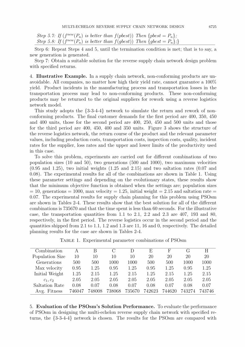
To solve this problem, experiments are carried out for different combinations of twopopulation sizes (10 and 50), two generations (500 and 1000), two maximum velocities(0.95 and 1.25), two initial weights (1.25 and 2.15) and two saltation rates (0.07 and0.08). The experimental results for all of the combinations are shown in Table 1. Usingthese parameter settings and depending on the evolutionary states, these results showthat the minimum objective function is obtained when the settings are; population sizes= 10, generations = 1000, max velocity = 1.25, initial weight = 2.15 and saltation rate =0.07. The experimental results for supply chain planning for this problem using PSOsmare shown in Tables 2-4. These results show that the best solution for all of the differentcombinations is 735670 and that the time spent is less than 60 seconds. For the illustrativecase, the transportation quantities from 1.1 to 2.1, 2.2 and 2.3 are 407, 193 and 80,respectively, in the first period. The reverse logistics occur in the second period and thequantities shipped from 2.1 to 1.1, 1.2 and 1.3 are 11, 16 and 0, respectively. The detailedplanning results for the case are shown in Tables 2-4.

Table 1. Experimental parameter combinations of PSOsm

Combination A B C D E F G HPopulation Size 10 10 10 10 20 20 20 20Generations 500 500 1000 1000 500 500 1000 1000Max velocity 0.95 1.25 0.95 1.25 0.95 1.25 0.95 1.25Initial Weight 1.25 2.15 1.25 2.15 1.25 2.15 1.25 2.15

c1, c2 2.05 2.05 2.05 2.05 2.05 2.05 2.05 2.05Saltation Rate 0.08 0.07 0.08 0.07 0.08 0.07 0.08 0.07Avg. Fitness 746047 748008 738068 735670 742623 744620 743274 743746

5. Evaluation of the PSOsm’s Solution Performance. To evaluate the performanceof PSOsm in designing the multi-echelon reverse supply chain network with specified re-turns, the {3-3-4-4} network is chosen. The results for the PSOsm are compared with


Figure 3. {3-3-4-4} reverse logistics network

those for the original GA and PSO. Table 5 shows the average value of the optimal pa-rameter combinations for the GA and PSO, after obtaining the solution for the parametercombination. As shown, for the PSO, the average fitness value of 736211 is the minimalaverage fitness value of the parameter combinations. The optimal parameter combina-tion is 10 particle populations, 1000 generation times, 1.25 maximal rate and 2.15 initial


Table 2. Production plan through PSOsm (1st period)

To Echelon 1 Echelon 2 Echelon 3 Echelon 4From P(1.1) P(1.2) P(1.3) P(2.1) P(2.2) P(2.3) P(3.1) P(3.2) P(3.3) P(3.4) P(4.1) P(4.2) P(4.3) P(4.4)

Echelon 1

P(1.1) 407 193 80P(1.2) 601 99 247P(1.3) 3 97 0

Echelon 2

P(2.1) 181 304 171 334P(2.2) 29 197 55 105P(2.3) 112 71 71 68

Echelon 3

P(3.1) 181 52 30 45P(3.2) 81 23 186 253P(3.3) 127 48 112 1P(3.4) 15 238 131 117

Table 3. Production plan through PSOsm (2nd period)


Echelon 1

P(1.1) 183 307 347P(1.2) 155 156 29P(1.3) Reverse 48 37 429

Echelon 2

P(2.1) 11 16 0 0 118 61 202P(2.2) 2 1 1 63 117 13 295P(2.3) 1 2 0 Reverse 67 507 87 123

Echelon 3

P(3.1) 5 1 3 12 0 61 52P(3.2) 9 6 2 167 128 274 139P(3.3) 3 1 1 14 40 85 16P(3.4) 8 3 2 Reverse 203 85 25 304

Echelon 4

P(4.1) 4 2 3 0P(4.2) 1 0 1 3P(4.3) 1 6 3 4P(4.4) 1 6 0 3

Demand 400 250 450 500

weight, with a linear decrease to 0.4 and 2.05 learning factors. The optimal parametercombination for the GA is a parent population of 10, 1000 generation times, 0.8 crossoverrate and 0.07 mutation rate. Its minimal average fitness is 739964. The average minimalfitness for the PSOsm of 735670, as shown in Table 5, is the smallest average fitness valueof the three algorithms. As can be seen, the average fitness value for the PSOsm is thelowest of the three algorithms.

Tables 6 and 7 show the verification and comparison data tables for the three algorithms.The data is collected from 30 iterations of independent calculations of the optimal param-eters and ANOVA verification is performed on the fitness value to check whether thereare significant differences. Shen and Hsieh [38] used a single factor ANOVA to verify thedifferences between the response of different visitors and various different projects at atourist attraction, in terms of satisfaction and loyalty. Scheffe’s Multiple Comparison testwas used to conduct the pairwise comparison [39-41]. If the diversity reaches a significantlevel, Scheffe’s multiple comparison test is used to verify the differences between differentgroups.

As shown in Table 6, the P-value is 1.65E-13, which is smaller than the confidencelevel, α (The mean difference is significant at the α = 0.05 level). Therefore, it can beinferred that the fitness values of these three algorithms display a significant variation,


Table 4. Production plan through PSOsm (3rd period)


Echelon 1

P(1.1) 46 75 316P(1.2) 132 135 42P(1.3) Reverse 596 216 141

Echelon 2

P(2.1) 4 4 1 93 304 91 266P(2.2) 4 2 0 95 93 1 225P(2.3) 5 0 7 Reverse 65 102 308 2

Echelon 3

P(3.1) 0 1 1 105 54 76 6P(3.2) 4 4 16 235 7 237 0P(3.3) 2 0 2 28 122 66 174P(3.4) 6 9 4 Reverse 19 279 18 173

Echelon 4

P(4.1) 1 7 1 8P(4.2) 0 1 0 1P(4.3) 2 7 2 1P(4.4) 1 4 0 8

Demand 400 450 400 350

Table 5. Experimental parameter combinations of PSO and GA

Combination A1 B1 C1 D1 E1 F1 G1 H1Population Size 10 10 10 10 20 20 20 20

PSO Generations 500 500 1000 1000 500 500 1000 1000Max velocity 0.95 1.25 0.95 1.25 0.95 1.25 0.95 1.25Initial Weight 1.25 2.15 1.25 2.15 1.25 2.15 1.25 2.15

c1, c2 2.05 2.05 2.05 2.05 2.05 2.05 2.05 2.05Avg. Fitness 757887 743386 739371 736211 746459 745624 746092 743423Combination A2 B2 C2 D2 E2 F2 G2 H2

Population Size 10 10 10 10 20 20 20 20GA Generations 500 500 1000 1000 500 500 1000 1000

Crossover Rate 0.75 0.8 0.75 0.8 0.75 0.8 0.75 0.8Mutation Rate 0.08 0.07 0.08 0.07 0.08 0.07 0.08 0.07Avg. Fitness 745835 747472 741094 739964 746964 745175 744937 745107

Table 6. Verified results for fitness value

Average VariancePSO 735899.8 6801490GA 740350.3 7841043PSOsm 734215.7 6844191P-value = 1.65E-13, Critical value = 3.101296

so Scheffe’s Multiple Comparison is used to conduct the pairwise comparison betweendifferent algorithms. Its formula is(

xi − xj −√(k − 1)Fα(k−1)(n−k)

√MSE

(1

ni

+1

nj

),

xi − xj +√(k − 1)Fα(k−1)(n−k)

√MSE

(1

ni

+1

nj

))


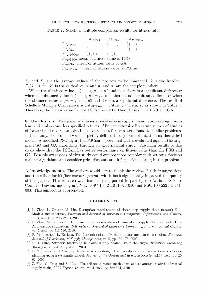
Table 7. Scheffe’s multiple comparison results for fitness value

FitµPSO FitµGA FitµPSOsm

FitµPSO (−,−) (+,+)FitµGA (−,−) (+,+)FitµPSOsm (+,+) (+,+)FitµPSO: mean of fitness value of PSOFitµGA: mean of fitness value of GAFitµPSOsm: mean of fitness value of PSOsm

Xi and Xj are the average values of the projects to be compared, k is the freedom,Fα(k − 1, n− k) is the critical value and ni and nj are the sample numbers.

When the obtained value is (+,+), µ1 > µ2 and that there is a significant difference;when the obtained value is (−,+), µ1 = µ2 and there is no significant difference; whenthe obtained value is (−,−), µ1 < µ2 and there is a significant difference. The result ofScheffe’s Multiple Comparison is FitµPSOsm < FitµPSO < FitµGA, as shown in Table 7.Therefore, the fitness value for the PSOsm is better than those of the PSO and GA.

6. Conclusions. This paper addresses a novel reverse supply chain network design prob-lem, which also considers specified returns. After an extensive literature survey of studiesof forward and reverse supply chains, very few references were found to similar problems.In this study, the problem was completely defined through an optimization mathematicalmodel. A modified PSO algorithm PSOsm is presented and is evaluated against the orig-inal PSO and GA algorithms, through an experimental study. The main results of thisstudy show that the PSOsm has better performance on fitness value than the PSO andGA. Possible extensions of this study could explore more complex multi-criteria decisionmaking algorithms and consider price discount and information sharing in the problem.

Acknowledgements. The authors would like to thank the reviews for their suggestionsand the editor for his/her encouragement, which both significantly improved the qualityof this paper. This research was financially supported in part by the National ScienceCouncil, Taiwan, under grant Nos. NSC 100-2410-H-027-010 and NSC 100-2221-E-141-003. This support is appreciated.

REFERENCES

[1] L. Zhao, L. Qu and M. Liu, Disruption coordination of closed-loop cupply chain network (I) –Models and theorems, International Journal of Innovative Computing, Information and Control,vol.4, no.11, pp.2955-2964, 2008.

[2] L. Zhao, M. Liu and L. Qu, Disruption coordination of closed-loop supply chain network (II) –Analysis and simulations, International Journal of Innovative Computing, Information and Control,vol.5, no.2, pp.511-520, 2009.

[3] R. Vrijhoel and L. Koskeia, The four roles of supply chain management in construction, EuropeanJournal of Purchasing & Supply Management, vol.6, pp.169-178, 2002.

[4] D. J. Flint, Strategic marketing in global supply chains: Four challenges, Industrial MarketingManagement, vol.33, pp.45-50, 2004.

[5] D. Y. Sha and Z. H. Che, Supply chain network design: Partner selection and production/distributionplanning using a systematic model, Journal of the Operational Research Society, vol.57, no.1, pp.52-62, 2006.

[6] Z. Yan, C. Teng and S. Miao, The self-organization mechanism and advantage analysis of virtualsupply chain, ICIC Express Letters, vol.4, no.2, pp.389-394, 2010.


[7] Z. H. Che and C. J. Chiang, A modified Pareto genetic algorithm for multi-objective build-to-ordersupply chain planning with product assembly, Advances in Engineering Software, vol.41, no.7-8,pp.1011-1022, 2010.

[8] H. Sadjady and H. Davoudpour, Two-echelon, multi-commodity supply chain network design withmode selection, lead-times and inventory costs, Computers & Operations Research, vol.39, no.7,pp.1345-1354, 2012.

[9] K. Das and A. H. Chowdhury, Designing a reverse logistics network for optimal collection, recoveryand quality-based product-mix planning, International Journal of Production Economics, vol.135,no.1, pp.209-221, 2012.

[10] S. Dowlatshahi, Developing a theory of reverse logistics, Interfaces, vol.30, no.3, pp.143-155, 2000.[11] L. H. Shih, Reverse logistics system planning for recycling electrical appliances and computers in

Taiwan, Conservation and Recycling, vol.32, pp.55-72, 2001.[12] A. Desai and A. Mital, Evaluation of disassemblability to enable design for disassembly in mass

production, International Journal of Industrial Ergonomics, vol.32, no.4, pp.265-281, 2003.[13] T. L. Hu, J. B. Sheu and K. H. Huang, A reverse logistics cost minimization model for the treatment

of hazardous wastes, Transportation Research Part E: Logistics Transportation Review, vol.38, no.6,pp.457-473, 2002.

[14] D. Imre, Optimal production-inventory strategies for a HMMS-type reverse logistics system, Inter-national Journal of Production Economics, vol.81-82, pp.351-360, 2003.

[15] D. S. Rogers and R. T. Lembke, An examination of reverse logistics practices, Journal of BusinessLogistics, vol.22, no.2, pp.129-148, 2001.

[16] P. J. Daugherty, C. W. Autry and A. E. Ellinger, Reverse logistics: The relationship between resourcecommitment and program performance, Journal of Business Logistics, vol.22, no.1, pp.107-123, 2001.

[17] M. Gen and R. Cheng, Genetic Algorithms and Engineering Design, Wiley, New York, 1997.[18] H. J. Ko and G. W. Evans, A genetic algorithm-based heuristic for the dynamic integrated for-

ward/reverse logistics network for 3PLs, Computers & Operational Research, vol.34, no.2, pp.346-366, 2007.

[19] D. Y. Sha and Z. H. Che, Virtual integration with a multi-criteria partner selection model for themulti-echelon manufacturing system, The International Journal of Advanced Manufacturing Tech-nology, vol.25, no.7-8, pp.739-802, 2005.

[20] H. Min, H. J. Ko and C. S. Ko, A genetic algorithm approach to developing the multi-echelon reverselogistics network for product returns, Omega, vol.34, no.1, pp.56-69, 2006.

[21] F. T. S. Chana, S. H. Chung and S. Wadhwa, A hybrid genetic algorithm for production anddistribution, Omega, vol.33, no.4, pp.345-355, 2005.

[22] F. van den Bergh and A. P. Engelbrecht, A study of particle swarm optimization particle trajectories,Information Sciences, vol.176, no.8, pp.937-971, 2006.

[23] C. C. Cui, B. Li and R. C. Zhang, Particle swarm optimization, Journal of Huaqiao University,vol.27, pp.343-346, 2006.

[24] F. H. Yu, H. B. Liu and J. B. Dai, Grey particle swarm algorithm for multi-objective optimizationproblems, Journal of Computer Applications, vol.26, no.12, pp.2950-2952, 2006.

[25] M. Clerc and J. Kennedy, The particle swarm: Explosion, stability, and convergence in a multi-dimensional complex space, IEEE Transactions on Evolutionary Computation, vol.6, no.1, pp.58-73,2002.

[26] S. He, Q. H. Wu, J. Y. Wen, J. R. Saunders and R. C. Paton, A particle swarm optimizer withpassive congregation, Biosystems, vol.78, no.1-3, pp.135-147, 2004.

[27] S. T. Wang and Z. J. Wang, Study of the application of PSO algorithms for nonlinear problems,Journal of Huazhong University of Science and Technology, vol.33, no.12, pp.4-7, 2005.

[28] H. J. Yu, L. P. Zhang, D. Z. Chen, X. F. Song and S. X. Hu, Estimation of model parameters usingcomposite particle swarm optimization, Journal of Chemical Engineering of Chinese Universities,vol.19, no.5, pp.675-680, 2005.

[29] Y. Luo, X. Yuan and Y. Liu, An improved PSO algorithm for solving non-convex NLP/MINLPproblems with equality constraints, Computers & Chemical Engineering, vol.31, no.3, pp.153-162,2006.

[30] Z. H. Che, Using fuzzy analytic hierarchy process and particle swarm optimization for balancedand defective supply chain problems considering WEEE/RoHS directives, International Journal ofProduction Research, vol.48, no.11, pp.3355-3381, 2010.

[31] A. Azadeh, M. S. Sangari and A. S. Amiri, A particle swarm algorithm for inspection optimizationin serial multi-stage processes, Applied Mathematical Modelling, vol.36, no.4, pp.1455-1464, 2012.


[32] Z. H. Che and Z. Cui, Unbalanced supply chain design using the analytic network process anda hybrid heuristic-based algorithm with balance modulating mechanism, International Journal ofBio-Inspired Computation, vol.3, no.1, pp.56-66, 2011.

[33] A. K. Sinha, H. K. Aditya, M. K. Tiwari and F. T. S. Chan, Agent oriented petroleum supply chaincoordination: Co-evolutionary particle swarm optimization based approach, Expert Systems withApplications, vol.38, no.5, pp.6132-6145, 2011.

[34] M. Mahnam, M. R. Yadollahpour, V. Famil-Dardashti and S. R. Hejazi, Supply chain modelingin uncertain environment with bi-objective approach, Computers & Industrial Engineering, vol.56,no.4, pp.1535-1544, 2009.

[35] M. F. Yang and Y. Lin, Applying the linear particle swarm optimization to a serial multi-echeloninventory model, Expert Systems with Applications, vol.37, no.3, pp.2599-2608, 2010.

[36] T. C. Jones and D. W. Riley, Using inventory for competitive advantage through supply chainmanagement, International Journal of Physical Distribution & Logistics Management, vol.15, no.5,pp.16-26, 1985.

[37] Y. Shi and R. Eberhart, A modified particle swarm optimizer, Proc. of IEEE International Confer-ence on Evolutionary Computation, pp.69-73, 1998.

[38] C. C. Shen and C. Y. Hsieh, A study on the relationship among attraction, tourist satisfaction andloyalty of religious tourism – A case of Fo Guang Shan in Kaohsiung, Tourism Management Research,vol.3, no.1, pp.79-95, 2003.

[39] H. Scheffe, A method for judging all contrasts in the analysis of variance, Biometrika, vol.40, no.1-2,pp.87-104, 1953.

[40] Y. H. Jou, Y. Y. Huang and H. N. Chen, Applying relationship marketing strategies to donors ofnon-profit organization: The case of social welfare charitable, Marketing Review, vol.2, no.1, pp.5-32,2005.

[41] S. Chou, C. S. Lin and Y. C. Hsieh, The influence on marketing performance of fit between marketingorganization characteristics and competitive strategies: Using the food industry as an example,Marketing Review, vol.2, no.1, pp.33-58, 2005.

multi-echelon reverse supply chain … · with specified returns using particle swarm optimization...

Documents