1

Multi-Layer Convolutional Sparse Modeling:Pursuit and Dictionary Learning

Jeremias Sulam, Member, IEEE, Vardan Papyan, Yaniv Romano, and Michael Elad Fellow, IEEE

Abstract—The recently proposed Multi-Layer ConvolutionalSparse Coding (ML-CSC) model, consisting of a cascade ofconvolutional sparse layers, provides a new interpretation ofConvolutional Neural Networks (CNNs). Under this framework,the forward pass in a CNN is equivalent to a pursuit algorithmaiming to estimate the nested sparse representation vectors from agiven input signal. Despite having served as a pivotal connectionbetween CNNs and sparse modeling, a deeper understandingof the ML-CSC is still lacking. In this work, we propose asound pursuit algorithm for the ML-CSC model by adoptinga projection approach. We provide new and improved boundson the stability of the solution of such pursuit and we analyzedifferent practical alternatives to implement this in practice.We show that the training of the filters is essential to allowfor non-trivial signals in the model, and we derive an onlinealgorithm to learn the dictionaries from real data, effectivelyresulting in cascaded sparse convolutional layers. Last, but notleast, we demonstrate the applicability of the ML-CSC modelfor several applications in an unsupervised setting, providingcompetitive results. Our work represents a bridge betweenmatrix factorization, sparse dictionary learning and sparse auto-encoders, and we analyze these connections in detail.

Index Terms—Convolutional Sparse Coding, Multilayer Pur-suit, Convolutional Neural Networks, Dictionary Learning,Sparse Convolutional Filters.

I. INTRODUCTION

New ways of understanding real world signals, and propos-ing ways to model their intrinsic properties, have led toimprovements in signal and image restoration, detection andclassification, among other problems. Little over a decade ago,sparse representation modeling brought about the idea thatnatural signals can be (well) described as a linear combinationof only a few building blocks or components, commonlyknown as atoms [1]. Backed by elegant theoretical results,this model led to a series of works dealing either with theproblem of the pursuit of such decompositions, or with thedesign and learning of better atoms from real data [2]. Thelatter problem, termed dictionary learning, empowered sparseenforcing methods to achieve remarkable results in manydifferent fields from signal and image processing [3], [4], [5]to machine learning [6], [7], [8].

Neural networks, on the other hand, were introduced aroundforty years ago and were shown to provide powerful classi-fication algorithms through a series of function compositions[9], [10]. It was not until the last half-decade, however, thatthrough a series of incremental modifications these methodswere boosted to become the state-of-the-art machine learning

J. Sulam, and M. Elad are with the Computer Science Department,Technion-Israel Institute of Technology. Y. Romano and V. Papyan are withthe Statistics Department of Stanford University.

tools for a wide range of problems, and across many differentfields [11]. For the most part, the development of new variantsof deep convolutional neural networks (CNNs) has been drivenby trial-and-error strategies and a considerable amount ofintuition.

Withal, a few research groups have begun providing the-oretical justifications and analysis strategies for CNNs fromvery different perspectives. For instance, by employing waveletfilters instead of adaptive ones, the work by Bruna and Mallat[12] demonstrated how scattering networks represent shiftinvariant analysis operators that are robust to deformations(in a Lipschitz-continuous sense). The inspiring work of [13]proposed a generative Bayesian model, under which typicaldeep learning architectures perform an inference process. In[14], the authors proposed a hierarchical tensor factorizationanalysis model to analyze deep CNNs. Fascinating connectionsbetween sparse modeling and CNN have also been proposed.In [15], a neural network architecture was shown to be ableto learn iterative shrinkage operators, essentially unrolling theiterations of a sparse pursuit. Building on this interpretation,the work in [16] further showed that CNNs can in fact improvethe performance of sparse recovery algorithms.

A precise connection between sparse modeling and CNNswas recently presented in [17], and its contribution is cen-tered in defining the Multi-Layer Convolutional Sparse Cod-ing (ML-CSC) model. When deploying this model to realsignals, compromises were made in way that each layer isonly approximately explained by the following one. With thisrelaxation in the pursuit of the convolutional representations,the main observation of that work is that the inference stageof CNNs – nothing but the forward-pass – can be interpretedas a very crude pursuit algorithm seeking for unique sparserepresentations. This is a useful perspective as it providesa precise optimization objective which, it turns out, CNNsattempt to minimize.

The work in [17] further proposed improved pursuits forapproximating the sparse representations of the network, orfeature maps, such as the Layered Basis Pursuit algorithm.Nonetheless, as we will show later, neither this nor theforward pass serve the ML-CSC model exactly, as they donot provide signals that comply with the model assumptions.In addition, the theoretical guarantees accompanying theselayered approaches suffer from bounds that become looserwith the network’s depth. The lack of a suitable pursuit, inturn, obscures how to properly sample from the ML-CSCmodel, and how to train the dictionaries from real data.

In this work we undertake a fresh study of the ML-CSC and of pursuit algorithms for signals in this model.

arX

iv:1

708.

0870

5v2

[cs

.CV

] 3

0 Ju

n 20

18

2

Our contributions will be guided by addressing the followingquestions:

1) Given proper convolutional dictionaries, how can oneproject1 signals onto the ML-CSC model?

2) When will the model allow for any signal to be expressedin terms of nested sparse representations? In other words,is the model empty?

3) What conditions should the convolutional dictionariessatisfy? and how can we adapt or learn them to representreal-world signals?

4) How is the learning of the ML-CSC model related totraditional CNN and dictionary learning algorithms?

5) What kind of performance can be expected from thismodel?

The model we analyze in this work is related to severalrecent contributions, both in the realm of sparse represen-tations and deep-learning. On the one hand, the ML-CSCmodel is tightly connected to dictionary constrained learningtechniques, such as Chasing Butterflies approach [18], fasttransform learning [19], Trainlets [20], among several others.On the other hand, and because of the unsupervised flavor ofthe learning algorithm, our work shares connections to sparseauto-encoders [21], and in particular to the k-sparse [22] andwinner-take-all versions [23].

In order to progressively answer the questions posed above,we will first review the ML-CSC model in detail in SectionII. We will then study how signals can be projected ontothe model in Section III, where we will analyze the stabilityof the projection problem and provide theoretical guaranteesfor practical algorithms. We will then propose a learningformulation in Section IV, which will allow, for the first time,to obtain a trained ML-CSC model from real data while beingperfectly faithful to the model assumptions. In this work werestrict our study to the learning of the model in an unsuper-vised setting. This approach will be further demonstrated onsignal approximation and unsupervised learning applicationsin Section V, before concluding in Section VI.

II. BACKGROUND

A. Convolutional Sparse Coding

The Convolutional Sparse Coding (CSC) model assumesa signal x ∈ RN admits a decomposition as D1γ1, whereγ1 ∈ RNm1 is sparse and D1 ∈ RN×Nm1 has a convolutionalstructure. More precisely, this dictionary consists of m1 localn1-dimensional filters at every possible location (Figure 1top). An immediate consequence of this model assumptionis the fact that each jth patch P0,jx ∈ Rn1 from thesignal x can be expressed in terms of a shift-invariant localmodel corresponding to a stripe from the global sparse vector,S1,jγ1 ∈ R(2n1−1)m1 . From now on, and for the sake ofsimplicity, we will drop the first index on the stripe and patchextraction operators, simply denoting the jth stripe from γ1

as Sjγ1.In the context of CSC, the sparsity of the representation

is better captured through the `0,∞ pseudo-norm [24]. This

1By projection, we refer to the task of getting the closest signal to the onegiven that obeys the model assumptions.

1

1 ∈ ℝ×1 ∈ ℝ1∈ ℝ

∈ ℝ1

1

2

1, ∈ ℝ 2 −1 1

1, ∈ ℝ 1

2 ∈ ℝ1×2 ∈ ℝ2

0,

1

1

1

1

2

1

1

1

2

2

Fig. 1: The CSC model (top), and its ML-CSC extension byimposing a similar model on γ1 (bottom).

measure, as opposed to the traditional `0, provides a notionof local sparsity and it is defined by the maximal number ofnon-zeros in a stripe from γ. Formally,

‖γ‖s0,∞ = maxi‖Siγ‖0. (1)

We kindly refer the reader to [24] for a more detailed descrip-tion of this model, as well as extensive theoretical guaranteesassociated with the model stability and the success of pursuitalgorithms serving it.

This model presents several characteristics that make itrelevant and interesting. On the one hand, CSC providesa systematic and formal way to develop and analyze verypopular and successful patch-based algorithms in signal andimage processing [24]. From a more practical perspective, onthe other hand, the convolutional sparse model has recentlyreceived considerable attention in the computer vision and ma-chine learning communities. Solutions based on the CSC havebeen proposed for detection [25], compressed sensing [26]texture-cartoon separation [27], [28], inverse problems [29],[30], [31] and feature learning [32], [33], and different con-volutional dictionary learning algorithms have been proposedand analyzed [29], [34], [35]. Interestingly, this model has alsobeen employed in a hierarchical way [36], [37], [38], [39]mostly following intuition and imitating successful CNNs’architectures. This connection between convolutional featuresand multi-layer constructions was recently made precise in theform of the Multi-Layer CSC model, which we review next.

B. Multi Layer CSC

The Multi-Layer Convolutional Sparse Coding (ML-CSC)model is a natural extension of the CSC described above, as itassumes that a signal can be expressed by sparse representa-tions at different layers in terms of nested convolutional filters.Suppose x = D1γ1, for a convolutional dictionary D1 ∈RN×Nm1 and an `0,∞-sparse representation γ1 ∈ RNm1 . Onecan cascade this model by imposing a similar assumption on

3

the representation γ1, i.e., γ1 = D2γ2, for a correspondingconvolutional dictionary D2 ∈ RNm1×Nm2 with m2 localfilters and a `0,∞-sparse γ2, as depicted in Figure 1. In thiscase, D2 is a also a convolutional dictionary with local filtersskipping m1 entries at a time2 – as there are m1 channels inthe representation γ1.

Because of this multi-layer structure, vector γ1 can beviewed both as a sparse representation (in the context ofx = D1γ1) or as a signal (in the context of γ1 = D2γ2). Thus,one one can refer to both its stripes (looking backwards topatches from x) or its patches (looking forward, correspondingto stripes of γ2). In this way, when analyzing the ML-CSCmodel we will not only employ the `0,∞ norm as definedabove, but we will also leverage its patch counterpart, wherethe maximum is taken over all patches from the sparse vectorby means of a patch extractor operator Pi. In order to maketheir difference explicit, we will denote them as ‖γ‖s0,∞and ‖γ‖p0,∞ for stripes and patches, respectively. In addition,we will employ the `2,∞ norm version, naturally defined as‖γ‖s2,∞ = max

i‖Siγ‖2, and analogously for patches.

We now formalize the model definition:

Definition 1. ML-CSC model:Given a set of convolutional dictionaries DiLi=1 of appropri-ate dimensions, a signal x(γi) ∈ RN admits a representationin terms of the ML-CSC model, i.e. x(γi) ∈Mλ, if

x = D1γ1, ‖γ1‖s0,∞ ≤ λ1,γ1 = D2γ2, ‖γ2‖s0,∞ ≤ λ2,

...γL−1 = DLγL, ‖γL‖s0,∞ ≤ λL.

Note that x(γi) ∈ Mλ can also be expressed as x =D1D2 . . .DLγL. We refer to D(i) as the effective dictionaryat the ith level, i.e., D(i) = D1D2 . . .Di. This way, one canconcisely write

x = D(i)γi, 1 ≤ i ≤ L. (2)

Interestingly, the ML-CSC can be interpreted as a specialcase of a CSC model: one that enforces a very specificstructure on the intermediate representations. We make thisstatement precise in the following Lemma:

Lemma 1. Given the ML-CSC model described by the setof convolutional dictionaries DiLi=1, with filters of spatialdimensions ni and channels mi, any dictionary D(i) =D1D2 . . .Di is a convolutional dictionary with mi local atomsof dimension neff

i =∑ij=1 nj − (i − 1). In other words, the

ML-CSC model is a structured global convolutional model.

The proof of this lemma is rather straight forward, and weinclude it in the Supplementary Material A. Note that what wasdenoted as the effective dimension at the ith layer is nothingelse than what is known in the deep learning community asthe receptive field of a filter at layer i. Here, we have madethis concept precise in the context of the ML-CSC model.

2This construction provides operators that are convolutional in the spacedomain, but not in the channel domain – just as for CNNs.

Fig. 2: From atoms to molecules: Illustration of the ML-CSCmodel for a number 6. Two local convolutional atoms (bottomrow) are combined to create slightly more complex structures– molecules – at the second level, which are then combinedto create the global atom representing, in this case, a digit.

As it was presented, the convolutional model assumes thatevery n-dimensional atom is located at every possible location,which implies that the filter is shifted with strides of s = 1.An alternative, which effectively reduces the redundancy of theresulting dictionary, is to consider a stride greater than one.In such case, the resulting dictionary is of size N ×Nm1/sfor one dimensional signals, and N × Nm1/s

2 for images.This construction, popular in the CNN community, does notalter the effective size of the filters but rather decreases thelength of each stripe by a factor of s in each dimension. In thelimit, when s = n1, one effectively considers non-overlappingblocks and the stripe will be of length3 m1 – the number oflocal filters. Naturally, one can also employ s > 1 for any ofthe multiple layers of the ML-CSC model. We will considers = 1 for all layers in our derivations for simplicity.

The ML-CSC imposes a unique structure on the globaldictionary D(L), as it provides a multi-layer linear compositionof simpler structures. In other words, D1 contains (small) localn1-dimensional atoms. The product D1D2 contains in each ofits columns a linear combination of atoms from D1, mergingthem to create molecules. Further layers continue to createmore complex constructions out of the simpler convolutionalbuilding blocks. We depict an example of such decompositionin Figure 2 for a 3rd-layer convolutional atom of the digit“6”. While the question of how to obtain such dictionaries willbe addressed later on, let us make this illustration concrete:consider this atom to be given by x0 = D1D2d3, where d3

is sparse, producing the upper-most image x0. Denoting byT (d3) = Supp(d3), this atom can be equally expressed as

x0 = D(2)d3 =∑

j∈T (d3)

d(2)j dj3. (3)

In words, the effective atom is composed of a few elementsfrom the effective dictionary D(2). These are the buildingblocks depicted in the middle of Figure 2. Likewise, focus-ing on the fourth of such atoms, d

(2)j4

= D1d2,j4 . In this

3When s = n1, the system is no longer shift-invariant, but rather invariantwith a shift of n samples.

4

particular case, ‖d2,j4‖0 = 2, so we can express d(2)j4

=

d(1)i1di12,j1 + d

(1)i2di22,j1 . These two atoms from D1 are precisely

those appearing in the bottom of the decomposition.

C. Pursuit in the noisy settingReal signals might contain noise or deviations from the

above idealistic model assumption, preventing us from en-forcing the above model exactly. Consider the scenario ofacquiring a signal y = x + v, where x ∈ Mλ and v is anuisance vector of bounded energy, ‖v‖2 ≤ E0. In this setting,the objective is to estimate all the representations γi whichexplain the measurements y up to an error of E0. In its mostgeneral form, this pursuit is represented by the Deep CodingProblem (DCPE

λ ), as introduced in [17]:

Definition 2. DCPEλ Problem:

For a global signal y, a set of convolutional dictionariesDiLi=1, and vectors λ and E:

(DCPEλ ) : find γiLi=1 s.t.

‖y −D1γ1‖2 ≤ E0, ‖γ1‖s0,∞ ≤ λ1‖γ1 −D2γ2‖2 ≤ E1, ‖γ2‖s0,∞ ≤ λ2

......

‖γL−1 −DLγL‖2 ≤ EL−1, ‖γL‖s0,∞ ≤ λL

where λi and Ei are the ith entries of λ and E , respectively.

The solution to this problem was shown to be stable interms of a bound on the `2-distance between the estimatedrepresentations γi and the true ones, γi. These results dependon the characterization of the dictionaries through their mutualcoherence, µ(D), which measures the maximal normalizedcorrelation between atoms in the dictionary. Formally, assum-ing the atoms are normalized as ‖di‖2 = 1 ∀i, this measureis defined as

µ(D) = maxi 6=j|dTi dj |. (4)

Relying on this measure, Theorem 5 in [17] shows that givena signal x(γi) ∈ PMλ

contaminated with noise of knownenergy E20 , if the representations satisfy the sparsity constraint

‖γi‖s0,∞ <1

2

(1 +

1

µ(Di)

), (5)

then the solution to the DCPEλ given by γiLi=1 satisfies

‖γi − γi‖22 ≤ 4E02i∏

j=1

4i−1

1− (2‖γj‖s0,∞ − 1)µ(Dj). (6)

In the particular instance of the DCPEλ where Ei = 0 for

1 ≤ i ≤ L − 1, the above bound can be made tighter by afactor of 4i−1 while preserving the same form.

These results are encouraging, as they show for the first timestability guarantees for a problem for which the forward passprovides an approximate solution. More precisely, if the abovemodel deviations are considered to be greater than zero (Ei >0) several layer-wise algorithms, including the forward pass ofCNNs, provide approximations to the solution of this problem[17]. We note two remarks about these stability results:

1) The bound increases with the number of layers or thedepth of the network. This is a direct consequence of thelayer-wise relaxation in the above pursuit, which causesthese discrepancies to accumulate over the layers.

2) Given the underlying signal x(γi) ∈ Mλ, with rep-resentations γiLi=1, this problem searches for theircorresponding estimates γiLi=1. However, because ateach layer ‖γi−1 −Diγi‖2 > 0, this problem does notprovide representations for a signal in the model. In otherwords, x 6= D1γ1, γ1 6= D2γ2, and generally x /∈Mλ.

III. A PROJECTION ALTERNATIVE

In this section we provide an alternative approach to theproblem of estimating the underlying representations γi underthe same noisy scenario of y = x(γi) + v. In particular, weare interested in projecting the measurements y onto the setMλ. Consider the following projection problem:

Definition 3. ML-CSC Projection PMλ:

For a signal y and a set of convolutional dictionaries DiLi=1,define the Multi-Layer Convolutional Sparse Coding projec-tion as:

(PMλ) : min

γiLi=1

‖y − x(γi)‖2 s.t. x(γi) ∈Mλ.

(7)

Note that this problem differs from the DCPEλ counterpart in

that we seek for a signal close to y, whose representationsγi give rise to x(γi) ∈ Mλ. This is more demanding (lessgeneral) than the formulation in the DCPE

λ . Put differently,the PMλ

problem can be considered as a special case of theDCPE

λ where model deviations are allowed only at the outer-most level. Recall that the theoretical analysis of the DCPE

λ

problem indicated that the error thresholds should increasewith the layers. Here, the PMλ

problem suggests a completelydifferent approach.

A. Stability of the projection PMλ

Given y = x(γi) + v, one can seek for the underlyingrepresentations γi through either the DCPE

λ or PMλproblem.

In light of the above discussion and the known stability resultfor the DCPE

λ problem, how close will the solution of thePMλ

problem be from the true set of representations? Theanswer is provided through the following result.

Theorem 4. Stability of the solution to the PMλproblem:

Suppose x(γi) ∈Mλ is observed through y = x + v, wherev is a bounded noise vector, ‖v‖2 ≤ E0, and ‖γi‖s0,∞ = λi <12

(1 + 1

µ(D(i))

), for 1 ≤ i ≤ L. Consider the set γiLi=1 to

be the solution of the PMλproblem. Then,

‖γi − γi‖22 ≤4E20

1− (2‖γi‖s0,∞ − 1)µ(D(i)). (8)

For the sake of brevity, we include the proof of this claimin the Supplementary Material B. However, we note a fewremarks:

1) The obtained bounds are not cumulative across the layers.In other words, they do not grow with the depth of thenetwork.

5

2) Unlike the stability result for the DCPEλ problem, the

assumptions on the sparse vectors γi are given in termsof the mutual coherence of the effective dictionaries D(i).Interestingly enough, we will see in the experimental sec-tion that one can in fact have that µ(D(i−1)) > µ(D(i)) inpractice; i.e., the effective dictionary becomes incoherentas it becomes deeper. Indeed, the deeper layers providelarger atoms with correlations that are expected to belower than the inner products between two small local(and overlapping) filters.

3) While the conditions imposed on the sparse vectorsγi might seem prohibitive, one should remember thatthis follows from a worst case analysis. Moreover, onecan effectively construct analytic nested convolutionaldictionaries with small coherence measures, as shown in[17].

Interestingly, one can also formulate bounds for the stabilityof the solution, i.e. ‖γi − γi‖22, which are the tightest for theinner-most layer, and then increase as one moves to shallowerlayers – precisely the opposite behavior of the solution to theDCPE

λ problem. This result, however, provides bounds that aregenerally looser than the one presented in the above theorem,and so we defer this to the Supplementary Material.

B. Pursuit AlgorithmsWe now focus on the question of how one can solve

the above problems in pracice. As shown in [17], one canapproximate the solution to the DCPE

λ in a layer-wise manner,solving for the sparse representations γi progressively fromi = 1, . . . , L. Surprisingly, the Forward Pass of a CNN isone such algorithm, yielding stable estimates. The LayeredBP algorithm was also proposed, where each representationγi is sparse coded (in a Basis Pursuit formulation) given theprevious representation γi−1 and dictionary Di. As solutionsto the DCPE

λ problem, these algorithms inherit the layer-wiserelaxation referred above, which causes the theoretical boundsto increase as a function of the layers or network depth.

Moving to the variation proposed in this work, how canone solve the PMλ

problem in practice? Applying the abovelayer-wise pursuit is clearly not an option, since after obtaininga necessarily distorted estimate γ1 we cannot proceed withequalities for the next layers, as γ1 does not necessarily havea perfectly sparse representation with respect to D2. Hereinwe present a simple approach based on a global sparse codingsolver which yields provable stable solutions.

Algorithm 1: ML-CSC Pursuit

Input: y, Di, k;

γL ← Pursuit(y,D(L), k);

for j = L, . . . , 1 doγj−1 ← Dj γj

return γi;

Consider Algorithm 1. This approach circumvents the prob-lem of sparse coding the intermediate features while guaran-

teeing their exact expression in terms of the following layer.This is done by first running a Pursuit for the deepest repre-sentation through an algorithm which provides an approximatesolution to the following problem:

minγ‖y −D(L)γ‖22 s.t. ‖γ‖s0,∞ ≤ k. (9)

Once the deepest representation has been estimated, weproceed by obtaining the remaining ones by simply applyingtheir definition, thus assuring that x = D(i)γi ∈ Mλ. Whilethis might seem like a dull strategy, we will see in the nextsection that, if the measurements y are close enough to a signalin the model, Algorithm 1 indeed provides stable estimatesγi. In fact, the resulting stability bounds will be shown tobe generally tighter than those existing for the layer-wisepursuit alternative. Moreover, as we will later see in the Resultssection, this approach can effectively be harnessed in practicein a real-data scenario.

C. Stability Guarantees for Pursuit Algorithms

Given a signal y = x(γi) + v, and the respective solutionof the ML-CSC Pursuit in Algorithm 1, how close will theestimated γi be to the original representations γi? Thesebounds will clearly depend on the specific Pursuit algorithmemployed to obtain γL. In what follows, we will present twostability guarantees that arise from solving this sparse codingproblem under two different strategies: a greedy and a convexrelaxation approach. Before diving in, however, we presenttwo elements that will become necessary for our derivations.

The first one is a property that relates to the propagation ofthe support, or non-zeros, across the layers. Given the supportof a sparse vector T = Supp(γ), consider dictionary DT asthe matrix containing only the columns indicated by T . Define‖DT ‖0∞ =

∑ni=1 ‖RiDT ‖0∞, where Ri extracts the ith row

of the matrix on its right-hand side. In words, ‖DT ‖0∞ simplycounts the number of non-zero rows of DT . With it, we nowdefine the following property:

Definition 5. Non Vanishing Support (N.V.S.):A sparse vector γ with support T satisfies the N.V.S propertyfor a given dictionary D if

‖Dγ‖0 = ‖DT ‖0∞. (10)

Intuitively, the above property implies that the entries in γwill not cause two or more atoms to be combined in such away that (any entry of) their supports cancel each other. Noticethat this is a very natural assumption to make. Alternatively,one could assume the non-zero entries from γ to be Gaussiandistributed, and in this case the N.V.S. property holds a.s.

A direct consequence of the above property is that ofmaximal cardinality of representations. If γ satisfies the N.V.Sproperty for a dictionary D, and γ is another sparse vectorwith equal support (i.e., Supp(γ) = Supp(γ)), then neces-sarily Supp(Dγ) ⊆ Supp(Dγ), and thus ‖Dγ‖0 ≥ ‖Dγ‖0.This follows from the fact that the number of non-zeros inDγ cannot be greater than the sum of non-zero rows from theset of atoms, DT .

6

The second element concerns the local stability of theStripe-RIP, the convolutional version of the Restricted Isomet-ric Property [40]. As defined in [24], a convolutional dictionaryD satisfies the Stripe-RIP condition with constant δk if, forevery γ such that ‖γ‖s0,∞ = k,

(1− δk)‖γ‖22 ≤ ‖Dγ‖22 ≤ (1 + δk)‖γ‖22. (11)

The S-RIP bounds the maximal change in (global) energyof a `0,∞-sparse vector when multiplied by a convolutionaldictionary. We would like to establish an equivalent propertybut in a local sense. Recall the ‖x‖p2,∞ norm, given by themaximal norm of a patch from x, i.e. ‖x‖p2,∞ = max

i‖Pix‖2.

Analogously, one can consider ‖γ‖s2,∞ = maxi‖Siγ‖2 to be

the maximal norm of a stripe from γ.Now, is ‖Dγ‖p2,∞ nearly isometric? The (partially affirma-

tive) answer is given in the form of the following Lemma,which we prove in the Supplementary Material C.

Lemma 2. Local one-sided near isometry property:If D is a convolutional dictionary satisfying the Stripe-RIPcondition in (11) with constant δk, then

‖Dγ‖2,p2,∞ ≤ (1 + δk) ‖γ‖2,s2,∞. (12)

This result is worthy in its own right, as it shows for thefirst time that not only the CSC model is globally stable for`0,∞-sparse signals, but that one can also bound the change inenergy in a local sense (in terms of the `2,∞ norm). While theabove Lemma only refers to the upper bound of ‖Dγ‖2,p2,∞,we conjecture that an analogous lower bound can be shownto hold as well.

With these elements, we can now move to the stability ofthe solutions provided by Algorithm 1:

Theorem 6. Stable recovery of the Multi-Layer Pursuit Algo-rithm in the convex relaxation case:Suppose a signal x(γi) ∈ Mλ is contaminated with locally-bounded noise v, resulting in y = x + v, ‖v‖p2,∞ ≤ ε0.Assume that all representations γi satisfy the N.V.S. propertyfor the respective dictionaries Di, and that ‖γi‖s0,∞ = λi <12

(1 + 1

µ(Di)

), for 1 ≤ i ≤ L and ‖γL‖s0,∞ = λL ≤

13

(1 + 1

µ(D(L))

). Let

γL = arg minγ‖y −D(L)γ‖|22 + ζL‖γ‖1, (13)

for ζL = 4ε0, and set γi−1 = Diγi, i = L, . . . , 1. Then,

1) Supp(γi) ⊆ Supp(γi),

2) ‖γi − γi‖p2,∞ ≤ εLL∏

j=i+1

√3cj2

,

hold for every layer 1 ≤ i ≤ L, where εL = 152 ε0

√‖γL‖p0,∞

is the error at the last layer, and cj depends on the ratiobetween the local dimensions of the layers, cj =

⌈2nj−1−1

nj

⌉.

Theorem 7. Stable recovery of the Multi-Layer Pursuit Algo-rithm in the greedy case:Suppose a signal x(γi) ∈ Mλ is contaminated with energy-bounded noise v, such that y = x + v, ‖y − x‖2 ≤ E0,

and ε0 = ‖v‖P2,∞. Assume that all representations γi satisfythe N.V.S. property for the respective dictionaries Di, with‖γi‖s0,∞ = λi <

12

(1 + 1

µ(Di)

), for 1 ≤ i ≤ L, and

‖γL‖s0,∞ <1

2

(1 +

1

µ(D(L))

)− 1

µ(D(L))· ε0|γminL |

, (14)

where γminL is the minimal entry in the support of γL.Consider approximating the solution to the Pursuit step inAlgorithm 1 by running Orthogonal Matching Pursuit for‖γL‖0 iterations. Then, for every ith layer,

1) Supp(γi) ⊆ Supp(γi),

2) ‖γi − γi‖22 ≤E20

1−µ(D(L))(‖γL‖s0,∞−1)

(32

)L−i.

The proofs of both Theorems 6 and 7 are included inthe Supplementary Material D1 and D2, respectively. Thecoefficient cj refers to the ratio between the filter dimensionsat consecutive layers, and assuming ni ≈ ni+1 (which indeedhappens in practice), this coefficient is roughly 2. Importantly,and unlike the bounds provided for the layer-wise pursuitalgorithm, the recovery guarantees are the tightest for theinner-most layer, and the bound increases slightly towardsshallower representations. The relaxation to the `1 norm, inthe case of the BP formulation, provides local error bounds,while the guarantees for the greedy version, in its OMPimplementation, yield a global alternative.

Before proceeding, one might wonder if the above con-ditions imposed on the representations and dictionaries aretoo severe and whether the set of signals satisfying these isempty. This is, in fact, not the case. As shown in [17], multi-layer convolutional dictionaries can be constructed by meansof certain wavelet functions, effectively achieving mutualcoherence values in the order of 10−3, leaving ample roomfor sampling sparse representations satisfying the theorems’assumptions. On the other hand, imposing a constraint on thenumber of non-zeros in a representation γi−1 = Diγi impliesthat part of the support of the atoms in Di will be required tooverlap. The N.V.S. property simply guarantees that wheneverthese overlaps occur, they will not cancel each other. Indeed,this happens with probability 1 if the non-zero coefficients aredrawn from a Normal distribution. We further comment andexemplify this in the Supplementary Material E.

D. Projecting General Signals

In the most general case, i.e. removing the assumption thaty is close enough to a signal in the model, Algorithm 1 byitself might not solve PMλ

. Consider we are given a generalsignal y and a model Mλ, and we run the ML-CSC Pursuitwith k = λL obtaining a set of representations γj. Clearly‖γL‖s0,∞ ≤ λL. Yet, nothing guarantees that ‖γi‖s0,∞ ≤ λifor i < L. In other words, in order to solve PMλ

one mustguarantee that all sparsity constraints are satisfied.

Algorithm 2 progressively recovers sparse representationsto provide a projection for any general signal y. The solutionis initialized with the zero vector, and then the OMP algorithmis applied with a progressively larger `0,∞ constraint on the

7

Algorithm 2: ML-CSC Projection Algorithm

Init: x∗ = 0 ;for k = 1 : λL do

γL ← OMP(y,D(L), k) ;for j = L : −1 : 1 do

γj−1 ← Dj γj ;

if ‖γi‖s0,∞ > λi for any 1 ≤ i < L thenbreak;

elsex∗ ← D(i)γi;

return x∗

deepest representation4, from 1 to λL. The only modificationrequired to run the OMP in this setting is to check at everyiteration the value of ‖γL‖s0,∞, and to stop accordingly. Ateach step, given the estimated γL, the intermediate featuresand their `0,∞ norms, are computed. If all sparsity constraintsare satisfied, then the algorithm proceeds. If, on the other hand,any of the constraints is violated, the previously computedx∗ is reported as the solution. Note that this algorithm canbe improved: if a constraint is violated, one might considerback-tracking the obtained deepest estimate and replacing thelast obtained non-zero by an alternative solution, which mightallow for the intermediate constraints to be satisfied. Forsimplicity, we present the completely greedy approach as inAlgorithm 2.

This algorithm can be shown to be a greedy approximationto an optimal algorithm, under certain assumptions, and weprovide a sketch of the proof of this claim in the Supple-mentary Material F. Clearly, while Algorithms 1 and 2 werepresented separately, they are indeed related and one cancertainly combine them into a single method. The distinctionbetween them was motivated by making the derivations of ourtheoretical analysis and guarantees easier to grasp. Neverthe-less, stating further theoretical claims without the assumptionof the signal y being close to an underlying x(γi) ∈ Mλ isnon-trivial, and we defer a further analysis of this case forfuture work.

E. Summary - Pursuit for the ML-CSC

Let us briefly summarize what we have introduced so far.We have defined a projection problem, PMλ

, seeking forthe closest signal in the model Mλ to the measurementsy. We have shown that if the measurements y are closeenough to a signal in the model, i.e. y = x(γi) + v, withbounded noise v, then the ML-CSC Pursuit in Algorithm 1manages to obtain approximate solutions that are not far fromthese representations, by deploying either the OMP or the BPalgorithms. In particular, the support of the estimated sparsevectors is guaranteed to be a subset of the correct support, andso all γi satisfy the model constraints. In doing so we have

4Instead of repeating the pursuit from scratch at every iteration, one might-warm start the OMP algorithm by employing current estimate, γL, as initialcondition so that only new non-zeros are added.

introduced the N.V.S. property, and we have proven that theCSC and ML-CSC models are locally stable. Lastly, if no priorinformation is known about the signal y, we have proposedan OMP-inspired algorithm that finds the closest signal x(γi)to any measurements y by gradually increasing the supportof all representations γi while guaranteeing that the modelconstraints are satisfied.

IV. LEARNING THE MODEL

The entire analysis presented so far relies on the assump-tion of the existence of proper dictionaries Di allowing forcorresponding nested sparse features γi. Clearly, the abilityto obtain such representations greatly depends on the designand properties of these dictionaries.

While in the traditional sparse modeling scenario certainanalytically-defined dictionaries (such as the Discrete CosineTransform) often perform well in practice, in the ML-CSCcase it is hard to propose an off-the-shelf construction whichwould allow for any meaningful decompositions. To see thismore clearly, consider obtaining γL with Algorithm 1 re-moving all other assumptions on the dictionaries Di. In thiscase, nothing will prevent γL−1 = DLγL from being dense.More generally, we have no guarantees that any collectionof dictionaries would allow for any signal with nested sparsecomponents γi. In other words, how do we know if the modelrepresented by DiLi=1 is not empty?

To illustrate this important point, consider the case whereDi are random – a popular construction in other sparsity-related applications. In this case, every atom from the dic-tionary DL will be a random variable djL ∼ N (0, σ2

LI). Inthis case, one can indeed construct γL, with ‖γL‖s0,∞ ≤ 2,such that every entry from γL−1 = DLγL will be a randomvariable γjL−1 ∼ N (0, σ2

L), ∀ j. Thus, Pr(γjL−1 = 0

)= 0.

As we see, there will not exist any sparse (or dense, for thatmatter) γL which will create a sparse γL−1. In other words,for this choice of dictionaries, the ML-CSC model is empty.

A. Sparse Dictionaries

From the discussion above one can conclude that one of thekey components of the ML-CSC model is sparse dictionaries:if both γL and γL−1 = DLγL are sparse, then atoms inD must indeed contain only a few non-zeros. We make thisobservation concrete in the following lemma.

Lemma 3. Dictionary Sparsity ConditionConsider the ML-CSC model Mλ described by the dic-tionaries DiLi=1 and the layer-wise `0,∞-sparsity levelsλ1, λ2, . . . , λL. Given γL : ‖γL‖s0,∞ ≤ λL and constants

ci =⌈2ni−1−1

ni

⌉, the signal x = D(L)γL ∈Mλ if

‖Di‖0 ≤λi−1λici

, ∀ 1 < i ≤ L. (15)

The simple proof of this Lemma is included in the Sup-plementary Material G. Notably, while this claim does nottell us if a certain model is empty, it does guarantee thatif the dictionaries satisfy a given sparsity constraint, one

8

can simply sample from the model by drawing the inner-most representations such that ‖γL‖s0,∞ ≤ λL. One questionremains: how do we train such dictionaries from real data?

B. Learning Formulation

One can understand from the previous discussion that thereis no hope in solving the PMλ

problem for real signalswithout also addressing the learning of dictionaries Di thatwould allow for the respective representations. To this end,considering the scenario where one is given a collection of Ktraining signals, ykKk=1, we upgrade the PMλ

problem to alearning setting in the following way:

minγk

i ,Di

K∑k=1

‖yk−xk(γki ,Di)‖22 s.t.

xk ∈Mλ,

‖dji‖2 = 1,∀ i, j.(16)

We have included the constraint of every dictionary atom tohave a unit norm to prevent arbitrarily small coefficients in therepresentations γki . This formulation, while complete, is diffi-cult to address directly: The constraints on the representationsγi are coupled, just as in the pursuit problem discussed in theprevious section. In addition, the sparse representations nowalso depend on the variables Di. In what follows, we providea relaxation of this cost function that will result in a simplelearning algorithm.

The problem above can also be understood from theperspective of minimizing the number of non-zeros in therepresentations at every layer, subject to an error threshold –a typical reformulation of sparse coding problems. Our mainobservation arises from the fact that, since γL−1 is functionof both DL and γL, one can upper-bound the number of non-zeros in γL−1 by that of γL. More precisely,

‖γL−1‖s0,∞ ≤ cL‖DL‖0‖γL‖s0,∞, (17)

where cL is a constant5. Therefore, instead of minimizing thenumber of non-zeros in γL−1, we can address the minimiza-tion of its upper bound by minimizing both ‖γL‖s0,∞ and‖DL‖0. This argument can be extended to any layer, and wecan generally write

‖γi‖s0,∞ ≤ c

L∏j=i+1

‖Dj‖0‖γL‖s0,∞. (18)

In this way, minimizing the sparsity of any ith representationcan be done implicitly by minimizing the sparsity of thelast layer and the number of non-zeros in the dictionariesfrom layer (i + 1) to L. Put differently, the sparsity of theintermediate convolutional dictionaries serve as proxies for thesparsity of the respective representation vectors. Following thisobservation, we now recast the problem in Equation (16) intothe following Multi-Layer Convolutional Dictionary Learning

5From [17], we have that ‖γL−1‖p0,∞ ≤ ‖DL‖0‖γL‖s0,∞. From here,and denoting by cL the upper-bound on the number of patches in a stripe fromγL−1 given by cL =

⌈2nL−1−1

nL

⌉, we can obtain a bound to ‖γL−1‖s0,∞.

Problem:

minγk

L,Di

K∑k=1

‖yk −D1D2 . . .DLγkL‖22 +

L∑i=2

ζi‖Di‖0

s.t.‖γkL‖s0,∞ ≤ λL,‖dji‖2 = 1,∀ i, j. (19)

Under this formulation, this problem seeks for sparse represen-tations γkL for each example yk, while forcing the intermediateconvolutional dictionaries (from layer 2 to L) to be sparse. Thereconstructed signal, x = D1γ1, is not expected to be sparse,and so there is no reason to enforce this property on D1. Notethat there is now only one sparse coding process involved –that of γkL – while the intermediate representations are nevercomputed explicitly. Recalling the theoretical results from theprevious section, this is in fact convenient as one only has toestimate the representation for which the recovery bound isthe tightest.

Following the theoretical guarantees presented in SectionIII, one can alternatively replace the `0,∞ constraint on thedeepest representation by a convex `1 alternative. The resultingformulation resembles the lasso formulation of the PMλ

problem, for which we have presented theoretical guarantees inTheorem 6. In addition, we replace the constraint on the `2 ofthe dictionary atoms by an appropriate penalty term, recastingthe above problem into a simpler (unconstrained) form:

minγk

L,Di

K∑k=1

‖yk −D1D2 . . .DLγkL‖22+

ι

L∑i=1

‖Di‖2F +

L∑i=2

ζi‖Di‖0 + λ‖γkL‖1, (20)

where ‖ · ‖F denotes the Frobenius norm. The problem inEquation (20) is highly non-convex, due to the `0 terms andthe product of the factors. In what follows, we present anonline alternating minimization algorithm, based on stochasticgradient descent, which seeks for the deepest representationγL and then progressively updates the layer-wise convolutionaldictionaries.

For each incoming sample yk (or potentially, a mini-batch),we will first seek for its deepest representation γkL consideringthe dictionaries fixed. This is nothing but the PMλ

problemin (7), which was analyzed in detail in the previous sections,and its solution will be approximated through iterative shrink-age algorithms. Also, one should keep in mind that whilerepresenting each dictionary by Di is convenient in termsof notation, these matrices are never computed explicitly –which would be prohibitive. Instead, these dictionaries (ortheir transpose) are applied effectively through convolutionoperators. In turn, this implies that images are not vectorizedbut processed as 2 dimensional matrices (or 3-dimensionaltensors for multi-channel images). In addition, these operatorsare very efficient due to their high sparsity, and one could inprinciple benefit from specific libraries to boost performancein this case, such as the one in [41].

Given the obtained γkL, we then seek to update the respectivedictionaries. As it is posed – with a global `0 norm over

9

a) b)

c)

Fig. 3: ML-CSC model trained on the MNIST dataset. a) The local filters of the dictionary D1. b) The local filters of theeffective dictionary D(2) = D1D2. c) Some of the 1024 local atoms of the effective dictionary D(3) which, because of thedimensions of the filters and the strides, are global atoms of size 28× 28.

each dictionary – this is nothing but a generalized pursuitas well. Therefore, for each dictionary Di, we minimize thefunction in Problem (20) by applying T iterations of projectedgradient descent. This is done by computing the gradient ofthe `2 terms in Problem (20) (call it f(Di)) with respectto a each dictionary Di (i.e., ∇f(Di)), making a gradientstep and then applying a hard-thresholding operation, Hζi(·),depending on the parameter ζi. This is simply an instance ofthe Iterative Hard Thresholding algorithm [42]. In addition,the computation of ∇f(Di) involves only multiplications theconvolutional dictionaries for the different layers. The overallalgorithm is depicted in Algorithm 3, and we will expand onfurther implementation details in the results section.

Algorithm 3: Multi-Layer Convolutional DictionaryLearning

Data: Training samples ykKk=1, initial convolutionaldictionaries DiLi=1

for k = 1, . . . ,K doDraw yk at random;Sparse Coding:γL ← arg min

γ‖yk −D(L)γ‖2 + λ‖γ‖1 ;

Update Dictonaries:for i = L, . . . , 2 do

for t = 1,. . . ,T doDt+1i ← Hζi [Dt

i − η∇f(Dti)] ;

for t = 1,. . . ,T doDt+1

1 ← Dt1 − η∇f(Dt

1) ;

The parameters of the models involve the `1 penalty ofthe deepest representation, i.e. λ, and the parameter for eachdictionary, ζi. The first parameter can be set manually or deter-mined so as to obtain a given given representation error. On theother hand, the dictionary-wise ζi parameters are less intuitiveto establish, and the question of how to set these values for agiven learning scenario remains a subject of current research.

Nevertheless, we will show in the experimental section thatsetting these manually results in effective constructions.

Note this approach can also be employed to minimizeProblem (19) by introducing minor modifications: In the sparsecoding stage, the Lasso is replaced by a `0,∞ pursuit, whichcan be tackled with a greedy alternative as the OMP (asdescribed in Theorem 7) or by an Iterative Hard Thresholdingalternative [42]. In addition, one could consider employingthe `1 norm as a surrogate for the `0 penalty imposed on thedictionaries. In this case, their update can still be performedby the same projected gradient descent approach, thoughreplacing the hard thresholding with its soft counterpart.

Before moving on, and even though an exhaustive compu-tational complexity analysis is out of the scope of this paper,we want to briefly comment on the general aspects of thealgorithm’s complexity. For a particular network architecture(number of layers, number of filters per layer, filter sizes, etc)let us denote by C the complexity of applying the forwardpass – or in other words, multiplying by D(L)T – on aninput image, or a minibach (i.e., for each kth iteration). Thesparse coding step in our algorithm is carried with iterativeshrinkage methods, and assuming these algorithms are run forτ iterations, the complexity incurred in each sparse coding stepis6 O(τC). The update of the dictionaries, on the other hand,requires computing the gradient for each set of filters. Each ofthese gradients involves, roughly speaking, the computation ofyet another forward and backward pass7. In this way, the dic-tionary update stage is O(LTC). Note that we are disregardingthe shrinkage operators both on the representations and onthe filters, which are entry-wise operations that are negligiblewhen compared to applying D(L) or its transpose. As canbe seen, the complexity of our algorithm is approximately

6Each such iteration actually involves the application of a forward andbackward pass, resulting from the fact that one needs to apply D(L) andD(L)T .

7The dictionary gradients can actually be computed more efficiently ifintermediate computations are saved (and stored), incurring in O(L log2(L))convolution operators. Thus, in this case the dictionary update stage isO(log2(L)TC). We defer the implementation of this more efficient algorithmfor future work.

10

(τ + TL) times that of a similar CNNs architectures. Finally,note that we are not considering the (important) fact that, inour case, the convolutional kernels are sparse, and as such theymay incur in significantly cheaper computations. This preciseanalysis, and how to maximize the related computationalbenefit, is left for future work.

C. Connection to related works

Naturally, the proposed algorithm has tight connections toseveral recent dictionary learning approaches. For instance,our learning formulation is closely related to the ChasingButterflies approach in [18], and our resulting algorithm canbe interpreted as a particular case of the FAUST method,proposed in the inspiring work from [43]. FAUST decomposeslinear operators into sparse factors in a hierarchical wayin the framework of a batch learning algorithm, resultingin improved complexity. Unlike that work, our multi-layerdecompositions are not only sparse but also convolutional, andthey are updated within a stochastic optimization framework.The work in [19], on the other hand, proposed a learningapproach where the dictionary is expressed as a cascade ofconvolutional filters with sparse kernels, and they effectivelyshowed how this approach can be used to approximate large-dimensional analytic atoms such as those from wavelets andcurvelets. As our proposed approach effectively learns a sparsedictionary, our work also shares similarities with the double-sparsity work from [44]. In particular, in its Trainlets version[20], the authors proposed to learn a dictionary as a sparsecombination of cropped wavelets atoms. From the previouscomment on the work from [19], this could also potentiallybe expressed as a product of sparse convolutional atoms.All these works, as well as our approach, essentially enforceextra regularization into the dictionary learning problem. Asa result, these methods perform better in cases with corruptedmeasurements, in high dimensional settings, and in cases withlimited amount of training data (see [44], [20]).

What is the connection between this learning formulationand that of deep convolutional networks? Recalling the analy-sis presented in [17], the Forward Pass is nothing but a layerednon-negative thresholding algorithm, the simplest form of apursuit for the ML-CSC model with layer-wise deviations.Therefore, if the pursuit for γL in our setting is solved withsuch an algorithm, then the problem in (20) implements aconvolutional neural network with only one RELU operatorat the last layer, with sparse-enforcing penalties on the filters.Moreover, due the data-fidelity term in our formulation, theproposed optimization problem provides nothing but a convo-lutional sparse autoencoder. As such, our work is related to theextensive literature in this topic. For instance, in [21], sparsityis enforced in the hidden activation layer by employing apenalty term proportional to the KL divergence between thehidden unit marginals and a target sparsity probability.

Other related works include the k-sparse autoencoders [22],where the hidden layer is constrained to having exactly k non-zeros. In practice, this boils down to a hard thresholding stepof the hidden activation, and the weights are updated withgradient descent. In this respect, our work can be thought

of a generalization of this work, where the pursuit algorithmis more sophisticated than a simple thresholding operation,and where the filters are composed by a cascade of sparseconvolutional filters. More recently, the work in [23] proposedthe winner-take-all autoencoders. In a nutshell, these are non-symmetric autoencoders having a few convolutional layers(with ReLu non-linearities) as the encoder, and a simple lineardecoder. Sparsity is enforced in what the authors refer to as“spatial” and a “lifetime” sparsity.

Finally, and due to the fact that our formulation effectivelyprovides a convolutional network with sparse kernels, ourapproach is reminiscent of works attempting to sparsify thefilters in deep learning models. For instance, the work in[41] showed that the weights of learned deep convolutionalnetworks can be sparsified without considerable degradationof classification accuracy. Nevertheless, one should perpendthe fact that these works are motivated merely by cheaper andfaster implementations, whereas our model is intrinsically builtby theoretically justified sparse kernels. We do not attemptto compare our approach to such sparsifying methods at thisstage, and we defer this to future work.

In light of all these previous works, the practical contribu-tion of the learning algorithm presented here is to demonstrate,as we will see in the following Experiments section, thatour online block-coordinate descent method can be effectivelydeployed in an unsupervised setting competing favorably withstate of the art dictionary learning and convolutional networkauto-encoders approaches.

V. EXPERIMENTS

We now provide experimental results to demonstrate severalaspects of the ML-CSC model. As a case-study, we considerthe MNIST dataset [45]. We define our model as consisting of3 convolutional layers: the first one contains 32 local filters ofsize 7× 7 (with a stride of 2), the second one consists of 128filters of dimensions 5 × 5 × 32 (with a stride of 1), and thelast one contains 1024 filters of dimensions 7×7×128. At thethird layer, the effective size of the atoms is 28 – representingan entire digit.

Training is performed with Algorithm 3, using a mini-batchof 100 samples per iteration. For the Sparse Coding stage,we leverage an efficient implementation of FISTA [46], andwe adjust the penalty parameter λ to obtain roughly 15 non-zeros in the deepest representation γ3. The ζi parameters,the penalty parameters for the dictionaries sparsity levels,are set manually for simplicity. In addition, and as it iscommonly done in various Gradient Descent methods, weemploy a momentum term for the update of the dictionariesDi within the projected gradient descent step in Algorithm3, and set its memory parameter to 0.9. The step size isset to 1, the update dictionary iterations is set as T = 1,ι = 0.001, and we run the algorithm for 20 epochs, whichtakes approximately 30 minutes. Our implementation uses theMatconvnet library, which leverages efficient functions forGPU8. No pre-processing was performed, with the exception

8All experiments are run on a 16 i7 cores Windows station with a NVIDIAGTX 1080 Ti.

11

0 5 10 15 20

Epochs

101

102

103

104

105Loss

0 5 10 15 20

Epoch

0.92

0.94

0.96

0.98

1DictionarydSparsity

D2

D3

0 5 10 15 20

Epochs

0.1

0.15

0.2

0.25AveragedResidual

Fig. 4: Evolution of the Loss function, sparsity of the convo-lutional dictionaries and average residual norm during trainingon the MNIST dataset.

of the subtraction of the mean image (computed on the trainingset).

We depict the evolution of the Loss function during trainingin Figure 4, as well as the sparsity of the second and thirddictionaries (i.e., 1 minus the number of non-zero coefficientsin the filters relative to the filters dimension) and the averageresidual norm. The resulting model is depicted in Figure 3.One can see how the first layer is composed of very simplesmall-dimensional edges or blobs. The second dictionary, D2,is effectively 99% sparse, and its non-zeros combine a fewatoms from D1 in order to create slightly more complex edges,as the ones in the effective dictionary D(2). Lastly, D3 is99.8% sparse, and it combines atoms from D(2) in order toprovide atoms that resemble different kinds (or parts) of digits.These final global atoms are nothing but a linear combinationof local small edges by means of convolutional sparse kernels.

Interestingly, we have observed that the mutual coherenceof the effective dictionaries do not necessarily increase withthe layers, and they often decrease with the depth. While thismeasure relates to worst-case analysis conditions and do notmean much in the context of practical performance, one cansee that the effective dictionary indeed becomes less correlatedas the depth increases. This is intuitive, as very simple edges– and at every location – are expected to show large innerproducts, larger than the correlation of two more complexnumber-like structures. This effect can be partially explainedby the dictionary redundancy: having 32 local filters in D1

(even while using a stride of 2) implies a 8-fold redundancy inthe effective dictionary at this level. This redundancy decreaseswith the depth (at this least for the current construction), andat the third layer one has merely 1024 atoms (redundancy ofabout 1.3, since the signal dimension is 282).

We can also find the multi-layer representation for realimages – essentially solving the projection problem PMλ

. InFigure 5, we depict the multi-layer features γi, i = 1, 2, 3,obtained with the Algorithm 1, that approximate an imagey (not included in the training set). Note that all the repre-sentations are notably sparse thanks to the very high sparsityof the dictionaries D2 and D3. These decompositions (anyof them) provide a sparse decomposition of the number 3 atdifferent scales, resulting in an approximation x. Naturally, thequality of the approximation can be improved by increasingthe cardinality of the representations.

Fig. 5: Decompositions of an image from MNIST in termsof its nested sparse features γi and multi-layer convolutionaldictionaries Di.

A. Sparse Recovery

The first experiment we explore is that of recovering sparsevectors from corrupted measurements, in which we will com-pare the presented ML-CSC Pursuit with the Layered approachfrom [17]. For the sake of completion and understanding, wewill first carry this experiment in a synthetic setting and thenon projected real digits, leveraging the dictionaries obtainedin the beginning of this section.

We begin by constructing a 3 layers “non-convolutional” 9

model for signals of length 200, with the dictionaries having250, 300, and 350 atoms, respectively. The first dictionary isconstructed as a random matrix, whereas the remaining onesare composed of sparse atoms with random supports and asparsity of 99%. Finally, 500 representations are sampled bydrawing sparse vectors γL, with a target sample sparsity kand normally distributed coefficients. We generate the signalsas x = D(i)γi, and then corrupt them with Gaussian noise(σ = 0.02) obtaining the measurements y = x(γi) + v.

In order to evaluate our projection approach, we run Algo-rithm 1 employing the Subspace Pursuit algorithm [47] for thesparse coding step, with the oracle target cardinality k. Recallthat once the deepest representations γL have been obtained,the inner ones are simply computed as γi−1 = Diγi. In thelayered approach from [17], on the other hand, the pursuitof the representations progresses sequentially: first running apursuit for γ1, then employing this estimate to run anotherpursuit for γ2, etc. In the same spirit, we employ SubspacePursuit layer by layer, employing the oracle cardinality ofthe representation at each stage. The results are presentedin Figure 6a: at the top we depict the relative `2 error ofthe recovered representations (‖γi − γi‖2/‖γi‖2) and, at thebottom, the normalized intersection of the supports [48], bothas a function of the sample cardinality k and the layer depth.

The projection algorithm manages to retrieve the representa-tions γi more accurately than the layered pursuit, as evidenced

9The non-convolutional case is still a ML-CSC model, in which the signaldimension is the same as the length of the atoms n, and with a stride of thesame magnitude n. We choose this setting for the synthetic experiment tosomewhat favor the results of the layered pursuit approach.

12

0 1 2 3

0

2

4

6

8

10 0

0.05

0.1

0.15

0.2

0.25

0.3

0 1 2 3

0

2

4

6

8

100.1

0.15

0.2

0.25

0.3

0 0.5 1 1.5 2 2.5 3

0

2

4

6

8

10 0

0.05

0.1

0.15

0.2

0 1 2 3

0

2

4

6

8

10 0

0.05

0.1

0.15

0.2

(a) Synthetic signals.

0 1 2 3

Layer

0

2

4

6

8

10

Sam

ple

Spa

rsity

0

0.1

0.2

0.3

0 1 2 3

Layer

0

2

4

6

8

10

Sam

ple

Spa

rsity

0.2

0.4

0.6

0.8

1

1.2

0 0.5 1 1.5 2 2.5 3

Layer

0

2

4

6

8

10

Sam

ple

Spa

rsity

0

0.2

0.4

0.6

0.8

0 1 2 3

Layer

0

2

4

6

8

10

Sam

ple

Spa

rsity

0

0.2

0.4

0.6

0.8

(b) MNIST signals.

Fig. 6: Recovery of representations from noisy MNIST digits.Top: normalized `2 error between the estimated and the truerepresentations. Bottom: normalized intersection between theestimated and the true support of the representations.

by the `2 error and the support recovery. The main reasonbehind the difficulty of the layer-by-layer approach is that theentire process relies on the correct recovery of the first layerrepresentations, γ1. If these are not properly estimated (asevidenced by the bottom-left graph), there is little hope for therecovery of the deeper ones. In addition, these representationsγ1 are the least sparse ones, and so they are expected to be themost challenging ones to recover. The projection alternative,on the other hand, relies on the estimation of the deepestγL, which are very sparse. Once these are estimated, theremaining ones are simply computed by propagating them tothe shallower layers. Following our analysis in the SectionIII-C, if the support of γL is estimated correctly, so will bethe support of the remaining representations γi.

We now turn to deploy the 3 layer convolutional dictionariesfor real digits obtained previously. To this end we take 500test digits from the MNIST dataset and project them on thetrained model, essentially running Algorithm 1 and obtaining

the representations γi. We then create the noisy measurementsas y = D(i)γi + v, where v is Gaussian noise with σ =0.02. We then repeat both pursuit approaches to estimate theunderlying representations, obtaining the results reported inFigure 6b.

Clearly, this represents a significantly more challengingscenario for the layered approach, which recovers only asmall fraction of the correct support of the sparse vectors.The projection algorithm, on the other hand, provides accurateestimations with negligible mistakes in the estimated supports,and very low `2 error. Note that the `2 error has little signif-icance for the Layered approach, as this algorithm does notmanage to find the true supports. The reason for the significantdeterioration in the performance of the Layered algorithm isthat this method actually finds alternative representations γ1,of the same sparsity, providing a lower fidelity term thanthe projection counterpart for the first layer. However, theseestimates γ1 do not necessarily provide a signal in the model,which causes further errors when estimating γ2.

B. Sparse Approximation

A straight forward application for unsupervised learnedmodel is that of approximation: how well can one approx-imate or reconstruct a signal given only a few k non-zerovalues from some representation? In this subsection, we studythe performance of the ML-CSC model for this task whilecomparing with related methods, and we present the resultsin Figure 7. The model is trained on 60K training examples,and the M-term approximation is measured on the remaining10K testing samples. All of the models are designed with 1Khidden units (or atoms).

Given the close connection of the ML-CSC model to sparseauto-encoders, we present the results obtained by approximat-ing the signals with sparse autoencoders [21] and k-sparseautoencoders [22]. In particular, the work in [21] trains sparseauto-encoders by penalizing the KL divergence between theactivation distribution of the hidden neurons and that of abinomial distribution with a certain target activation rate. Assuch, the resulting activations are never truly sparse. Forthis reason, since the M-term approximation is computed bypicking the highest entries in the hidden neurons and settingthe remaining ones to zero, this method exhibits a considerablerepresentation error.

K-sparse auto-encoders perform significantly better, thoughthey are sensitive to the number of non-zeros used duringtraining. Indeed, if the model is trained with 25 non-zerosper sample, the model performs well for a similar rangeof cardinalities. Despite this sensitivity on training, theirperformance is remarkable considering the simplicity of thepursuit involved: the reconstruction is done by computingx = Wγk + b′, where γk is a k-sparse activation (or feature)obtained by hard thresholding as γk = Hk

[WTy + b

], and

where b and b′ are biases vectors. Note that while a convolu-tional multi-layer version of this family of autoencoders wasproposed in [23], these constructions are trained in stackedmanner – i.e., training the first layer independently, thentraining the second one to represent the features of the first

13

0 10 20 30 40 50 60 70 80 90 100

NNZ

0.05

0.1

0.15

0.2

0.25

0.3R

elat

ived

Rec

onst

ruct

iond

Err

or

SparsedAutoEncoderML-CSCdyIncreasingdSparsity)k-SparsedAEdy25-50-60)Trainlets

0.05

0.13

1.360.35

0.010.006

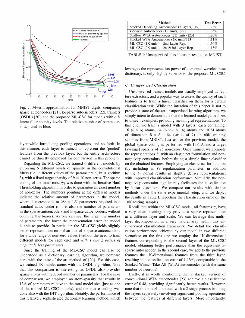
Fig. 7: M-term approximation for MNIST digits, comparingsparse autoencoders [21], k-sparse autoencoders [22], trainlets(OSDL) [20], and the proposed ML-CSC for models with dif-ferent filter sparsity levels. The relative number of parametersis depicted in blue.

layer while introducing pooling operations, and so forth. Inthis manner, each layer is trained to represent the (pooled)features from the previous layer, but the entire architecturecannot be directly employed for comparison in this problem.

Regarding the ML-CSC, we trained 6 different models byenforcing 6 different levels of sparsity in the convolutionalfilters (i.e., different values of the parameters ζi in Algorithm3), with a fixed target sparsity of k = 10 non-zeros. The sparsecoding of the inner-most γ3 was done with the Iterative HardThresholding algorithm, in order to guarantee an exact numberof non-zeros. The numbers pointing at the different modelsindicate the relative amount of parameters in the model,where 1 corresponds to 282 × 1K parameters required in astandard autoencoder (this is also the number of parametersin the sparse-autoencoders and k-sparse autoencoders, withoutcounting the biases). As one can see, the larger the numberof parameters, the lower the representation error the modelis able to provide. In particular, the ML-CSC yields slightlybetter representation error than that of k-sparse autoencoders,for a wide range of non-zero values (without the need to traindifferent models for each one) and with 1 and 2 orders ofmagnitude less parameters.

Since the training of the ML-CSC model can also beunderstood as a dictionary learning algorithm, we comparehere with the state-of-the-art method of [20]. For this case,we trained 1K trainlet atoms with the OSDL algorithm. Notethat this comparison is interesting, as OSDL also providessparse atoms with reduced number of parameters. For the sakeof comparison, we employed an atom-sparsity that results in13% of parameters relative to the total model size (just as oneof the trained ML-CSC models), and the sparse coding wasdone also with the IHT algorithm. Notably, the performance ofthis relatively sophisticated dictionary learning method, which

Method Test ErrorStacked Denoising Autoencoder (3 layers) [49] 1.28%k-Sparse Autoencoder (1K units) [22] 1.35%Shallow WTA Autoencoder (2K units) [23] 1.20%Stacked WTA Autoencoder (2K units)[23] 1.11%ML-CSC (1K units) - 2nd Layer Rep. 1.30%ML-CSC (2K units) - 2nd&3rd Layer Rep. 1.15%

TABLE I: Unsupervised classification results on MNIST.

leverages the representation power of a cropped wavelets basedictionary, is only slightly superior to the proposed ML-CSC.

C. Unsupervised Classification

Unsupervised trained models are usually employed as fea-ture extractors, and a popular way to assess the quality of suchfeatures is to train a linear classifier on them for a certainclassification task. While the intention of this paper is not toprovide a state-of-the-art unsupervised learning algorithm, wesimply intent to demonstrate that the learned model generalizesto unseen examples, providing meaningful representations. Tothis end, we train a model with 3 layers, each containing:16 (5 × 5) atoms, 64 (5 × 5 × 16) atoms and 1024 atomsof dimension 5 × 5 × 64 (stride of 2) on 60K trainingsamples from MNIST. Just as for the previous model, theglobal sparse coding is performed with FISTA and a target(average) sparsity of 25 non-zeros. Once trained, we computethe representations γi with an elastic net formulation and non-negativity constraints, before fitting a simple linear classifieron the obtained features. Employing an elastic-net formulation(by including an `2 regularization parameter, in additionto the `1 norm) results in slightly denser representations,with improved classification performance. Similarly, the non-negativity constraint significantly facilitates the classificationby linear classifiers. We compare our results with similarmethods under the same experimental setup, and we depictthe results in Table I, reporting the classification error on the10K testing samples.

Recall that within the ML-CSC model, all features γi havea very clear meaning: they provide a sparse representationat a different layer and scale. We can leverage this multi-layer decomposition in a very natural way within this un-supervised classification framework. We detail the classifi-cation performance achieved by our model in two differentscenarios: on the first one we employ the 1K-dimensionalfeatures corresponding to the second layer of the ML-CSCmodel, obtaining better performance than the equivalent k-sparse autoencoder. In the second case, we add to the previousfeatures the 1K-dimensional features from the third layer,resulting in a classification error of 1.15%, comparable to theStacked Winner Take All (WTA) autoencoder (with the samenumber of neurons).

Lastly, it is worth mentioning that a stacked version ofconvolutional WTA autoencoder [23] achieve a classificationerror of 0.48, providing significantly better results. However,note that this model is trained with a 2-stage process (trainingthe layers separately) involving significant pooling operationsbetween the features at different layers. More importantly,

14

the features computed by this model are 51,200-dimensional(more than an order of magnitude larger than in the othermodels) and thus cannot be directly compared to the re-sults reporter by our method. In principle, similar stacked-constructions that employ pooling could be built for our modelas well, and this remains as part of ongoing work.

VI. CONCLUSION

We have carefully revisited the ML-CSC model and ex-plored the problem of projecting a signal onto it. In doingso, we have provided new theoretical bounds for the solutionof this problem as well as stability results for practical algo-rithms, both greedy and convex. The search for signals withinthe model led us to propose a simple, yet effective, learningformulation adapting the dictionaries across the different layersto represent natural images. We demonstrated the proposedapproach on a number of practical applications, showing thatthe ML-CSC can indeed provide significant expressivenesswith a very small number of model parameters.

Several question remain open: how should the model bemodified to incorporate pooling operations between the layers?what consequences, both theoretical and practical, would thishave? How should one recast the learning problem in orderto address supervised and semi-supervised learning scenarios?Lastly, we envisage that the analysis provided in this work willempower the development of better practical and theoreticaltools not only for structured dictionary learning approaches,but to the field of deep learning and machine learning ingeneral.

VII. ACKNOWLEDGMENTS

The research leading to these results has received fundingfrom the European Research Council under European UnionsSeventh Framework Programme, ERC Grant agreement no.320649. J. Sulam kindly thanks J. Turek for fruitful discus-sions.

REFERENCES

[1] A. M. Bruckstein, D. L. Donoho, and M. Elad, “From Sparse Solutionsof Systems of Equations to Sparse Modeling of Signals and Images,”SIAM Review., vol. 51, pp. 34–81, Feb. 2009.

[2] R. Rubinstein, A. M. Bruckstein, and M. Elad, “Dictionaries for sparserepresentation modeling,” IEEE Proceedings - Special Issue on Applica-tions of Sparse Representation & Compressive Sensing, vol. 98, no. 6,pp. 1045–1057, 2010.

[3] J. Sulam, B. Ophir, and M. Elad, “Image Denoising Through Multi-Scale Learnt Dictionaries,” in IEEE International Conference on ImageProcessing, pp. 808 – 812, 2014.

[4] Y. Romano, M. Protter, and M. Elad, “Single image interpolation viaadaptive nonlocal sparsity-based modeling,” IEEE Trans. on ImageProcess., vol. 23, no. 7, pp. 3085–3098, 2014.

[5] J. Mairal, F. Bach, and G. Sapiro, “Non-local Sparse Models for Im-age Restoration,” IEEE International Conference on Computer Vision.,vol. 2, pp. 2272–2279, 2009.

[6] Z. Jiang, Z. Lin, and L. S. Davis, “Label consistent k-svd: Learning adiscriminative dictionary for recognition,” Pattern Analysis and MachineIntelligence, IEEE Transactions on, vol. 35, no. 11, pp. 2651–2664,2013.

[7] V. M. Patel, Y.-C. Chen, R. Chellappa, and P. J. Phillips, “Dictionariesfor image and video-based face recognition,” JOSA A, vol. 31, no. 5,pp. 1090–1103, 2014.

[8] A. Shrivastava, V. M. Patel, and R. Chellappa, “Multiple kernel learningfor sparse representation-based classification,” IEEE Transactions onImage Processing, vol. 23, no. 7, pp. 3013–3024, 2014.

[9] Y. LeCun, B. E. Boser, J. S. Denker, D. Henderson, R. E. Howard, W. E.Hubbard, and L. D. Jackel, “Handwritten digit recognition with a back-propagation network,” in Advances in neural information processingsystems, pp. 396–404, 1990.

[10] D. E. Rumelhart, G. E. Hinton, R. J. Williams, et al., “Learningrepresentations by back-propagating errors,” Cognitive modeling, vol. 5,no. 3, p. 1, 1988.

[11] Y. LeCun, Y. Bengio, and G. Hinton, “Deep learning,” Nature, vol. 521,no. 7553, pp. 436–444, 2015.

[12] J. Bruna and S. Mallat, “Invariant scattering convolution networks,”IEEE transactions on pattern analysis and machine intelligence, vol. 35,no. 8, pp. 1872–1886, 2013.

[13] A. B. Patel, T. Nguyen, and R. G. Baraniuk, “A probabilistic theory ofdeep learning,” arXiv preprint arXiv:1504.00641, 2015.

[14] N. Cohen, O. Sharir, and A. Shashua, “On the expressive power of deeplearning: A tensor analysis,” in 29th Annual Conference on LearningTheory (V. Feldman, A. Rakhlin, and O. Shamir, eds.), vol. 49 ofProceedings of Machine Learning Research, (Columbia University, NewYork, New York, USA), pp. 698–728, PMLR, 23–26 Jun 2016.

[15] K. Gregor and Y. LeCun, “Learning fast approximations of sparse cod-ing,” in Proceedings of the 27th International Conference on MachineLearning (ICML-10), pp. 399–406, 2010.

[16] B. Xin, Y. Wang, W. Gao, D. Wipf, and B. Wang, “Maximal sparsitywith deep networks?,” in Advances in Neural Information ProcessingSystems, pp. 4340–4348, 2016.

[17] V. Papyan, Y. Romano, and M. Elad, “Convolutional neural networksanalyzed via convolutional sparse coding,” The Journal of MachineLearning Research, vol. 18, no. 1, pp. 2887–2938, 2017.

[18] L. Le Magoarou and R. Gribonval, “Chasing butterflies: In search ofefficient dictionaries,” in IEEE Int. Conf. Acoust. Speech, Signal Process,Apr. 2015.

[19] O. Chabiron, F. Malgouyres, J. Tourneret, and N. Dobigeon, “TowardFast Transform Learning,” International Journal of Computer Vision,pp. 1–28, 2015.

[20] J. Sulam, B. Ophir, M. Zibulevsky, and M. Elad, “Trainlets: Dictionarylearning in high dimensions,” IEEE Transactions on Signal Processing,vol. 64, no. 12, pp. 3180–3193, 2016.

[21] A. Ng, “Sparse autoencoder,” CS294A Lecture notes, vol. 72, no. 2011,pp. 1–19, 2011.

[22] A. Makhzani and B. Frey, “K-sparse autoencoders,” arXiv preprintarXiv:1312.5663, 2013.

[23] A. Makhzani and B. J. Frey, “Winner-take-all autoencoders,” in Ad-vances in Neural Information Processing Systems, pp. 2791–2799, 2015.

[24] V. Papyan, J. Sulam, and M. Elad, “Working locally thinking globally:Theoretical guarantees for convolutional sparse coding,” IEEE Transac-tions on Signal Processing, vol. 65, no. 21, pp. 5687–5701, 2017.

[25] P. Sermanet, K. Kavukcuoglu, S. Chintala, and Y. LeCun, “Pedestriandetection with unsupervised multi-stage feature learning,” in ComputerVision and Pattern Recognition (CVPR), 2013 IEEE Conference on,pp. 3626–3633, IEEE, 2013.

[26] K. Li, L. Gan, and C. Ling, “Convolutional compressed sensing usingdeterministic sequences,” IEEE Transactions on Signal Processing,vol. 61, no. 3, pp. 740–752, 2013.

[27] H. Zhang and V. M. Patel, “Convolutional sparse coding-based imagedecomposition.,” in BMVC, 2016.

[28] H. Zhang and V. M. Patel, “Convolutional sparse and low-rank coding-based image decomposition,” IEEE Transactions on Image Processing,vol. 27, no. 5, pp. 2121–2133, 2018.

[29] V. Papyan, Y. Romano, J. Sulam, and M. Elad, “Convolutional dictionarylearning via local processing,” in The IEEE International Conference onComputer Vision (ICCV), Oct 2017.

[30] F. Heide, W. Heidrich, and G. Wetzstein, “Fast and flexible convolutionalsparse coding,” in Computer Vision and Pattern Recognition (CVPR),2015 IEEE Conference on, pp. 5135–5143, IEEE, 2015.

[31] B. Choudhury, R. Swanson, F. Heide, G. Wetzstein, and W. Heidrich,“Consensus convolutional sparse coding,” in Computer Vision (ICCV),2017 IEEE International Conference on, pp. 4290–4298, IEEE, 2017.

[32] M. Henaff, K. Jarrett, K. Kavukcuoglu, and Y. LeCun, “Unsupervisedlearning of sparse features for scalable audio classification.,” in ISMIR,vol. 11, p. 2011, Citeseer, 2011.

[33] A. D. Szlam, K. Gregor, and Y. L. Cun, “Structured sparse codingvia lateral inhibition,” in Advances in Neural Information ProcessingSystems, pp. 1116–1124, 2011.

15

[34] B. Wohlberg, “Efficient algorithms for convolutional sparse representa-tions,” IEEE Transactions on Image Processing, vol. 25, pp. 301–315,Jan. 2016.

[35] J. Liu, C. Garcia-Cardona, B. Wohlberg, and W. Yin, “Online convolu-tional dictionary learning,” arXiv preprint arXiv:1709.00106, 2017.

[36] M. D. Zeiler, D. Krishnan, G. W. Taylor, and R. Fergus, “Deconvolu-tional networks,” in Computer Vision and Pattern Recognition (CVPR),2010 IEEE Conference on, pp. 2528–2535, IEEE, 2010.

[37] A. Szlam, K. Kavukcuoglu, and Y. LeCun, “Convolutional matchingpursuit and dictionary training,” arXiv preprint arXiv:1010.0422, 2010.

[38] K. Kavukcuoglu, P. Sermanet, Y.-L. Boureau, K. Gregor, M. Mathieu,and Y. L. Cun, “Learning convolutional feature hierarchies for visualrecognition,” in Advances in neural information processing systems,pp. 1090–1098, 2010.

[39] Y. He, K. Kavukcuoglu, Y. Wang, A. Szlam, and Y. Qi, “Unsupervisedfeature learning by deep sparse coding,” in Proceedings of the 2014SIAM International Conference on Data Mining, pp. 902–910, SIAM,2014.

[40] E. J. Candes and T. Tao, “Decoding by linear programming,” InformationTheory, IEEE Transactions on, vol. 51, no. 12, pp. 4203–4215, 2005.

[41] B. Liu, M. Wang, H. Foroosh, M. Tappen, and M. Pensky, “Sparseconvolutional neural networks,” in Proceedings of the IEEE Conferenceon Computer Vision and Pattern Recognition, pp. 806–814, 2015.

[42] T. Blumensath and M. E. Davies, “Iterative Thresholding for SparseApproximations,” Journal of Fourier Analysis and Applications, vol. 14,pp. 629–654, Sept. 2008.

[43] L. Le Magoarou and R. Gribonval, “Flexible multilayer sparse approxi-mations of matrices and applications,” IEEE Journal of Selected Topicsin Signal Processing, vol. 10, no. 4, pp. 688–700, 2016.

[44] R. Rubinstein, M. Zibulevsky, and M. Elad, “Double Sparsity : LearningSparse Dictionaries for Sparse Signal Approximation,” IEEE Trans.Signal Process., vol. 58, no. 3, pp. 1553–1564, 2010.

[45] Y. LeCun, L. Bottou, Y. Bengio, and P. Haffner, “Gradient-based learningapplied to document recognition,” Proceedings of the IEEE, vol. 86,no. 11, pp. 2278–2324, 1998.

[46] A. Beck and M. Teboulle, “A fast iterative shrinkage-thresholding algo-rithm for linear inverse problems,” SIAM journal on imaging sciences,vol. 2, no. 1, pp. 183–202, 2009.

[47] W. Dai and O. Milenkovic, “Subspace pursuit for compressive sens-ing signal reconstruction,” IEEE Transactions on Information Theory,vol. 55, no. 5, pp. 2230–2249, 2009.

[48] M. Elad, Sparse and Redundant Representations: From Theory toApplications in Signal and Image Processing. Springer PublishingCompany, Incorporated, 1st ed., 2010.

[49] P. Vincent, H. Larochelle, I. Lajoie, Y. Bengio, and P.-A. Manzagol,“Stacked denoising autoencoders: Learning useful representations in adeep network with a local denoising criterion,” Journal of MachineLearning Research, vol. 11, no. Dec, pp. 3371–3408, 2010.

APPENDIX

A. Properties of the ML-CSC model

Lemma 1. Given the ML-CSC model described by the setof convolutional dictionaries DiLi=1, with filters of spatialdimensions ni and channels mi, any dictionary D(i) =D1D2 . . .Di is a convolutional dictionary with mi local atomsof dimension neff

i =∑ij=1 nj − (i − 1). In other words, the

ML-CSC model is a structured global convolutional model.

Proof. A convolutional dictionary is formally defined as theconcatenation of banded circulant matrices. Consider D1 =[C

(1)1 ,C

(1)2 , . . . ,C

(1)m1

], where each circulant C

(1)i ∈ RN×N .

Likewise, one can express D2 =[C

(2)1 ,C

(2)2 , . . . ,C

(2)m2

],

where C(2)i ∈ RNm1×N . Then,

D(2) = D1D2 =[D1C

(2)1 ,D1C

(2)2 , . . . ,D1C

(2)m2

]. (21)

Each term D1C(2)i is the product of a concatenation of banded

circulant matrices and a banded circulant matrix. Because theatoms in each C

(2)i have a stride of m1 (the number of filters

+ − 1

()

()

Fig. 8: Illustration of a convolutional dictionary D1 multipliedby one of the circulat matrices from D2, in this case C

(2)1 .

in D1) each of these products is in itself a banded circulantmatrix. This is illustrated in Figure 8, where it becomes clearthat the first atom in C

(2)1 (of length n2m1) linearly combines

atoms from the first n2 blocks of m1 filters in D1 (in thiscase n2 = 2). These block are simply the unique set of filtersshifted at every position. The second column in C

(2)1 will do

the same for the next set n2 blocks, starting from the secondone, etc.

From the above discussion, D1C(2)1 results in a banded

circulant matrix of dimension N ×N . In particular, the bandof this matrix is given by the dimension of the filters in thefirst dictionary (n1) plus the number of blocks combined byC

(2)1 minus one. In other words, the effective dimension of

the filters in D1C(2)1 is given by neff

2 = n2 + n1 − 1.The effective dictionary D(2) = D1D2 is simply a concate-

nation of m2 such banded circulant matrices. In other words,D(2) is a convolutional dictionary with filters of dimensionneff2 . The same analysis can be done for the effective dictionary

at every layer, D(i), resulting in an effective dimension ofneffi = ni + neff

i−1 − 1, and so neffL =

∑Li=1 ni − (L− 1).

Finally, note that D(i) has Nmi columns, and thus therewill be mi local filters in the effective CSC model.

B. Stability result for the PMλproblem

Theorem 4. Stability of the solution to the PMλproblem:

Suppose x(γi) ∈Mλ is observed through y = x + v, wherev is a bounded noise vector, ‖v‖2 ≤ E0, and ‖γi‖s0,∞ = λi <12

(1 + 1

µ(D(i))

), for 1 ≤ i ≤ L. Consider the set γiLi=1 to

be the solution of the PMλproblem. Then,

‖γi − γi‖22 ≤4E20

1− (2‖γi‖s0,∞ − 1)µ(D(i)). (22)

Proof. Denote the solution to the PMλproblem by x; i.e.,

x = D(i)γi. Given that the original signal x satisfies ‖y −x‖2 ≤ E0, the solution to the PMλ

problem, x must satisfy

‖y − x‖2 ≤ ‖y − x‖2 ≤ E0, (23)

as this is the signal which provides the shortest `2 (data-fidelity) distance from y. Note that because x(γi) ∈Mλ, wecan have that x = D(i)γi, ∀ 1 ≤ i ≤ L. Recalling Lemma 1,the product D1D2 . . .Di is a convolutional dictionary. In addi-tion, we have required that ‖γi‖s0,∞ ≤ λi < 1

2

(1 + 1

µ(D(i))

).

16

Therefore, from the same arguments presented in [24], itfollows that

‖γi − γi‖22 ≤4E20

1− (2‖γi‖s0,∞ − 1)µ(D(i)). (24)

Theorem 9. (Another stability of the solution to the PMλ

problem):Suppose x(γi) ∈ Mλ is observed through y = x + v,where v is a bounded noise vector, ‖v‖2 ≤ E0, and 10

‖γi‖s0,∞ = λi <12

(1 + 1

µ(Di)

), for 1 ≤ i ≤ L. Consider

the set γiLi=1 to be the solution of the PMλproblem. If

‖γL‖s0,∞ < 12

(1 + 1

µ(D(L))

)then

‖γi − γi‖22 ≤4E20

1− (2‖γL‖s0,∞ − 1)µ(D(L))

L∏j=i+1

[1 + (2‖γj‖s0,∞ − 1)µ(Dj)

]. (25)

Proof. Given that the original signal x satisfies ‖y−x‖2 ≤ E0,the solution to the PMλ

problem, x must satisfy

‖y − x‖2 ≤ ‖y − x‖2 ≤ E0, (26)

as this is the signal which provides a lowest `2 (data-fidelity)term. In addition, ‖γL‖s0,∞ = λL <

12 (1+ 1

µ(D(L))). Therefore,

from the same arguments presented in [24], it follows that

‖γL − γL‖22 ≤4E20

1− (2‖γL‖s0,∞ − 1)µ(D(L))= E2L. (27)

Because the solution x(γi) ∈ Mλ, then γL−1 = DLγL.Therefore

‖γL−1− γL−1‖22 = ‖DL(γL− γL)‖22 ≤ (1+δ2k)‖γL− γL‖22,(28)

where δ2k is the S-RIP of DL with constant 2k = 2‖γL‖s0,∞.This follows from the triangle inequality of the `0,∞ normand the fact that, because γL is a solution to the PMλ

problem, ‖γL‖s0,∞ ≤ λL = ‖γL‖s0,∞. The S-RIP can inturn be bounded with the mutual coherence [24] as δk ≤(k − 1)µ(DL), from which one obtains

‖γL−1 − γL−1‖22 ≤ E2L (1 + (2‖γL‖s0,∞ − 1)µ(DL)). (29)

From similar arguments, extending this to an arbitrary ith

layer,

‖γi − γi‖22 ≤ E2LL∏

j=i+1

(1 + (2‖γj‖s0,∞ − 1)µ(Dj)). (30)

For the sake of simplicity, one can relax the above boundsfurther obtaining that, subject to the assumptions in Theorem4,

‖γi − γi‖22 ≤ E2L 2(L−i). (31)

10The assumption that ‖γi‖s0,∞ = λi can be relaxed to ‖γi‖s0,∞ ≤ λi,with slight modifications of the result.

This follows simply by employing the fact that ‖γi‖s0,∞ <12

(1 + 1

µ(Di)

).

C. Local stability of the S-RIP

Lemma 2. Local one-sided near isometry:If D is a convolutional dictionary satisfying the Stripe-RIPcondition with constant δk, then

‖Dγ‖2,p2,∞ ≤ (1 + δk) ‖γ‖2,s2,∞ (32)

Proof. Consider the patch-extraction operator Pi from thesignal x = Dγ, and Si the operator that extracts the cor-responding stripe from γ such that Pix = ΩSiγ, whereΩ is a local stripe dictionary [24]. Denote the ith stripe bysi = Siγ. Furthermore, denote by Si the operator that extractsthe support of si from γ. Clearly, x = DSTi Siγ. Note that‖Pi‖2 = ‖Si‖2 = 1. Then,

‖Dγ‖p2,∞ = maxi‖PiDSTi Siγ‖2 (33)

≤ maxi‖Pi‖2 ‖DSTi Siγ‖2 (34)

≤ maxi‖DSTi ‖2‖Siγ‖2 (35)

≤ maxi‖DSTi ‖2 max

j‖Sjγ‖2. (36)

Note that

maxj‖Sjγ‖2 = max

j‖Sjγ‖2 = ‖γ‖s2,∞, (37)

as the non-zero entries in Sjγ and Sjγ are the same. On theother hand, denoting by λmax(·) the maximal eigenvalue ofthe matrix in its argument, ‖DSTi ‖2 =

√λmax

(SiDTDSTi

),

and if T = Supp(γ),

λmax(SiD

TDSTi)≤ λmax

(DTTDT

), (38)

because11 SiDTDSTi is a principal sub-matrix of DT

TDT .Thus, also ‖DSTi ‖2 ≤ ‖DT ‖2.

The Stripe-RIP condition, as in Equation (11), provides abound on the square of the singular values of DT . Indeed,‖DT ‖22 ≤ (1 + δk), for every T : ‖T ‖s0,∞ = k. Includingthese in the above one obtains the desired claim:

‖Dγ‖p2,∞ ≤ maxi‖DSTi ‖2 max

j‖Sjγ‖2 ≤

√1 + δk‖γ‖s2,∞.

(39)

D. Recovery guarantees for pursuit algorithms

1) Convex relaxation case:

Theorem 6. Stable recovery of the Multi-Layer Pursuit Algo-rithm in the convex relaxation case:Suppose a signal x(γi) ∈ Mλ is contaminated with locally-bounded noise v, resulting in y = x + v, ‖v‖p2,∞ ≤ ε0.Assume that all representations γi satisfy the N.V.S. property

11The inequality in (38) can be shown by considering the equivalentexpression λmax

(SiD

TTDT S

Ti

), where the matrix DT

TDT is real andsymmetric, and the matrix Si is semi-orthogonal; i.e. SiSTi = I. Thus, fromPoincare Separation Theorem, λmin

(DTTDT

)≤ λ

(SiD

TTDτSTi

)≤

λmax(DTTDT

).

17

for the respective dictionaries Di, and that ‖γi‖s0,∞ = λi <12

(1 + 1

µ(Di)

), for 1 ≤ i ≤ L and ‖γL‖s0,∞ = λL ≤

13

(1 + 1

µ(D(L))

). Consider solving the Pursuit stage in Al-

gorithm 1 as

γL = arg minγ‖y + D(L)γ‖|22 + ζL‖γ‖1, (40)

for ζL = 4ε0, and set γi−1 = Diγi, i = L, . . . , 1. Then, forevery 1 ≤ i ≤ L layer,

1) Supp(γi) ⊆ Supp(γi),

2) ‖γi − γi‖p2,∞ ≤ εLL∏

j=i+1

√3cj2

,

where εL = 152 ε0

√‖γj‖p0,∞ is the error at the last layer, and

cj is a coefficient that depends on the ratio between the localdimensions of the layers, cj =

⌈2nj−1−1

nj

⌉.

Proof. Denote ∆i = γi − γi. From [24] (Theorem 19), thesolution γL will satisfy:

i) S(γL) ⊆ S(γL); andii) ‖∆L‖∞ ≤ 15

2 ε0.As shown in [17], given the `∞ bound of the representation

error, we can bound its `2,∞ norm as well, obtaining

‖∆L‖p2,∞ ≤ ‖∆L‖∞√‖∆L‖p0,∞ ≤

15

2ε0

√‖γL‖p0,∞, (41)

because, since S(γL) ⊂ S(γL), ‖∆L‖s0,∞ ≤ ‖γL‖s0,∞.

Define εL = 152 ε0

√‖γL‖p0,∞.

Recall that the N.V.S. property states that the entries in γwill no cause the support of the atoms in D cancel each other;i.e., ‖Dγ‖0 = ‖DT ‖0∞ (Definition 5). In other words, thisprovides a bound on the cardinality of the vector resulting fromthe multiplication of D with any sparse vector with support T .Concretely, if γ satisfies the N.V.S., then ‖Dγ‖0 ≥ ‖Dγ‖0.

Consider now the estimate at the L − 1 layer, obtained asγL−1 = DLγL. Because γL satisfies the N.V.S. property, andS(γL) ⊆ S(γL), then ‖γL−1‖0 ≤ ‖γL−1‖0, and more soS(γL−1) ⊆ S(γL−1).

On the other hand, recalling Lemma 2 and denoting by δλL

the Stripe-RIP constant of the DL dictionary, and because‖∆L‖s0,∞ ≤ ‖γL‖s0,∞ ≤ λL,

‖∆L−1‖2,p2,∞ = ‖DL∆L‖2,p2,∞ ≤ (1 + δλL)‖∆L‖2,s2,∞. (42)

Notice that by employing the above Lemma, we havebounded the patch-wise `2,∞ norm of ∆L−1 in terms ofthe stripe-wise `2,∞ of ∆L. Recalling the derivation from[17] (Section 7.1), at each ith layer, a stripe includes up to(2ni−1 − 1)/ni patches. Define ci =

⌈2ni−1−1

ni

⌉. From this,

one can bound the square of the `2 norm of a stripe with thenorm of the maximal patch within it - this is true for everystripe, and in particular for the stripe with the maximal norm.This implies that ‖∆L‖2,s2,∞ ≤ cL‖∆L‖2,p2,∞. Then,

‖∆L−1‖2,p2,∞ ≤ (1 + δk)‖∆L‖2,s2,∞ ≤ (1 + δλL)cL‖∆L‖2,p2,∞.

(43)Employing the result in Eq. (41),

‖∆L−1‖2,p2,∞ ≤ (1 + δk)cL‖∆L‖2,p2,∞ ≤ (1 + δk) cL ε2L. (44)

We can further bound the Stripe-RIP constant by δk ≤ (k −1)µ(D) [24], obtaining

‖∆L−1‖2,p2,∞ ≤ (1 + (‖γL‖s0,∞ − 1)µ(DL)) ε2L cL. (45)

Iterating this analysis for the remaining layers yields

‖γi−γi‖2,p2,∞ ≤ ε2LL∏

j=i+1

cj (1+(‖γj‖s0,∞−1)µ(Dj)). (46)

This general result can be relaxed for the sake of simplicity.Indeed, considering that ‖γi‖s0,∞ < 1

2

(1 + 1

µ(Di)

), for 1 ≤

i ≤ L,1 + (‖γj‖s0,∞ − 1)µ(Dj) < 3/2, (47)

and so

‖γi − γi‖p2,∞ ≤ εLL∏

j=i+1

√3cj2

(48)

2) Greedy case:

Theorem 7. Stable recovery of the Multi-Layer Pursuit Algo-rithm in the greedy case:Suppose a signal x(γi) ∈ Mλ is contaminated with energy-bounded noise v, such that y = x + v, ‖y − x‖2 ≤ E0,and ε0 = ‖v‖P2,∞. Assume that all representations γi satisfythe N.V.S. property for the respective dictionaries Di, with‖γi‖s0,∞ = λi <

12

(1 + 1

µ(Di)

), for 1 ≤ i ≤ L, and

‖γL‖s0,∞ <1

2

(1 +

1

µ(D(L))

)− 1

µ(D(L))· ε0|γminL |

, (49)

where γminL is the minimal entry in the support of γL.Consider approximating the solution to the Pursuit step inAlgorithm 1 by running Orthogonal Matching Pursuit for‖γL‖0 iterations. Then

1) Supp(γi) ⊆ Supp(γi),2) ‖γi − γi‖22 ≤

E201−µ(D(L))(‖γL‖s0,∞−1)

(32

)L−i.

Proof. Given that γL satisfies Equation (49), from [24] (The-orem 17) one obtains that

‖γL − γL‖22 ≤E20

1− µ(D(L))(‖γL‖s0,∞ − 1). (50)

Moreover, if the OMP algorithm is run for ‖γL‖0 iterations,then all the non-zero entries are recovered, i.e., Supp(γL) =Supp(γL). Therefore, ‖γL − γL‖s0,∞ ≤ ‖γL‖s0,∞ = λL.

Now, let γL−1 = DLγL. Regarding the support ofγL−1, because γL satisfies the N.V.S. property, ‖γL−1‖0 ≤‖γL−1‖0. More so, all entries in γL−1 will correspond to non-zero entries in γL−1. In other words,

Supp(γL−1) ⊆ Supp(γL−1). (51)

Consider now the error at the L−1 layer, ‖γL−1− γL−1‖22.Since ‖γL−1 − γL−1‖s0,∞ ≤ ‖γL−1‖s0,∞, we can bound thiserror in terms of the Stripe RIP:

‖γL−1−γL−1‖22 = ‖DL(γL−γL)‖22 ≤ (1+δλL)‖γL−γL‖22,

(52)

18

We can further bound the SRIP constant as δk ≤ (k−1)µ(D),from which one obtains

‖γL−1 − γL−1‖22 ≤E20 (1 + (‖γL‖s0,∞ − 1)µ(DL))

1− µ(D(L))(‖γL‖s0,∞ − 1). (53)

From similar arguments, one obtains analogous claims for anyith layer; i.e.,

‖γi − γi‖22 ≤E20

1− µ(D(L))(‖γL‖s0,∞ − 1)

L∏j=i+1

(1 + (‖γj‖s0,∞ − 1)µ(Dj)). (54)

This bound can be further relaxed for the sake of simplicity.Because ‖γi‖s0,∞ < 1

2

(1 + 1

µ(Di)

), for 1 ≤ i ≤ L, then

(1 + (‖γL‖s0,∞ − 1)µ(DL)) < 3/2, and so

‖γi − γi‖22 ≤E20

1− µ(D(L))(‖γL‖s0,∞ − 1)

(3

2

)L−i. (55)

E. Discussion on Theorem 6 and Theorem 7

In this section, we elaborate and comment further on theconditions impossed in the above theorems, regarding both theallowed sparsity and the N.V.S. property. While the conditionsof Theorems 6 and 7 might appear restrictive, the set ofrepresentations and dictionaries satisfying these conditions arenot empty. An example of such constructions can be found inreference [17], where multi-layer overcomplete convolutionaldictionaries are constructed by employing shifted versions ofa discrete Meyer wavelet. This way, the resulting dictionarieshave mutual coherence values in the order of 10−3 and 10−4,which provide ample room for sampling sparse representationssatisfying the theorems assumptions.

Regarding the NVS assumption, we stress that this is not asprohibitive as it might seem, and it is only needed because ourtheorems consider a deterministic worst-case scenario. Let usexemplify this better: consider a representation γ2 with 5 non-zero coefficients, and a dictionary D2 composed of atoms with3 non-zeros each, uniformly distributed. If the entries in allnon-zero coefficients are sampled from a normal distribution,the resulting inner representations γ1 = D2γ2 will havecardinalities in the range [3, 15]. If the mutual-coherence ofD1 is such that the allowed maximal number of non-zeros perstripe (i.e., the `0,∞ norm) is, say, 7 (an assumption that issatisfied by the cases explained above), then this implies thatthe only signals that are allowed to exist are those composedof atoms with some overlaps of their support. The NVSassumption only implies that whenever these overlaps occur,they will not cancel each other. This, in fact, occurs withprobability 1 if the non-zero coefficients are sampled froma Gaussian distribution.

We further depict this example in Figure 9. Note how thenumber of non-zeros in γ1 is not allowed to be as large aspossible (i.e., it is constrained to be below 7 by means ofoverlapping supports). The NVS property simply assumes that

the coefficients multiplying d2 and d3 will not be such thatthe entry marked with red dotted line is zero.

Fig. 9: Illustration of the propagation of supports accrossrepresentations. See comments in the text.

F. Projecting General Signals

The method depicted in Algorithm 2 can be shown to be agreedy approximation to an optimal algorithm, under certainassumptions, and we now provide a sketch of the proof of thisclaim. Consider the first iteration of the above method, wherek = 1. If OMP succeeds in providing the closest γL subjectto the respective constraint, i.e. providing the solution to

minγ‖y −D(L)γ‖22 s.t. ‖γ‖s0,∞ ≤ 1, (56)

and if ‖γi‖s0,∞ ≤ λi for every i, then this solution effectivelyprovides the closest signal to y in the model defined byλ = [λ1, . . . , 1]. If λL = 1, we are done. Otherwise, if λL > 1,we might increase the number of non-zeros in γL, whiledecreasing the `2 distance to y. This is done by continuingto the next iteration: running again OMP with the constraint‖γL‖s0,∞ ≤ 2, and obtaining the respective γi.

At any kth iteration, due to the nature of the OMP algo-rithm, Supp(γk−1L ) ⊆ Supp(γkL). If all estimates γi satisfythe N.V.S. property for the respective dictionaries Di, thenthe sparsity of each γi is non-decreasing through the iterations,‖γk−1i ‖s0,∞ ≤ ‖γki ‖s0,∞. For this reason, if an estimate γkL isobtained such that any of the corresponding `0,∞ constraints isviolated, then necessarily one constraint will be violated at thenext (or any future) iteration. Therefore, the algorithm outputsthe signal corresponding to the iteration before one of theconstraints was violated. A complete optimal (combinatorial)algorithm would need to retrace its steps and replace the lastnon-zero added to γkL by the second best option, and thenevaluate if all constraints are met for this selection of thesupport. This process should be iterated, and Algorithm 2provides a greedy approximation to this idea.

G. Sparse Dictionaries

Lemma 3. Dictionary Sparsity ConditionConsider the ML-CSC model Mλ described by the thedictionaries D1Li=1 and the layer-wise `0,∞-sparsity levels

19

λ1, λ2, . . . , λL. Given γL : ‖γL‖s0,∞ ≤ λL and constants

ci =⌈2ni−1−1

ni

⌉, the signal x = D(L)γL ∈Mλ if

‖Di‖0 ≤λi−1λici

, ∀ 1 < i ≤ L. (57)

Proof. This lemma can be proven simply by consideringthat the patch-wise `0,∞ of the representation γL−1 canbe bounded by ‖γL−1‖p0,∞ ≤ ‖DL‖0‖γL‖s0,∞. Thus, if‖DL‖0 ≤ λL−1/λL and ‖γL‖s0,∞ ≤ λL, then ‖γL−1‖p0,∞ ≤λL−1. Recalling the argument in [17] (Section 7.1), a stripefrom the ith layer includes up to ci = d(2ni−1 − 1)/niepatches. Therefore, ‖γL−1‖s0,∞ ≤ cL‖γL−1‖

p0,∞, and so γL−1

will satisfy its corresponding sparsity constraint if ‖DL‖0 ≤λL−1/(cLλL). Iterating this argument for the remaining layersproves the above lemma.