multi-objectives, multi-period optimization of district ... · pdf filemulti-objectives,...
TRANSCRIPT
Multi-Objectives, Multi-Period Optimization of district
energy systems: I-Selection of typical operating periods
Samira Fazlollahia,b,⇤, Stephane Laurent Bungenerb, Pierre Mandelc,Gwenaelle Beckera, Francois Marechalb
aVeolia Environnement Recherche et Innovation (VERI), 291 avenue Dreyfous Ducas,78520 Limay, France
bIndustrial Process and Energy Systems Engineering, Ecole Polytechnique Federale deLausanne, CH-1015 Lausanne, Switzerland
cVeolia Environnement Recherche et Innovation (VERI), Chemin de la digue BP 76,78603 Maisons-La�tte, France
Abstract
The long term optimization of a district energy system is a computation-ally demanding task due to the large number of data points representing theenergy demand profiles.
In order to reduce the number of data points and therefore the compu-tational load of the optimization model, this paper presents a systematicprocedure to reduce a complete data set of the energy demand profiles intoa limited number of typical periods, which adequately preserve significantcharacteristics of the yearly profiles. The proposed method is based on theuse of a k-means clustering algorithm assisted by an ✏-constraints optimiza-tion technique. The proposed typical periods allow us to achieve the accuraterepresentation of the yearly consumption profiles, while significantly reducingthe number of data points.
The work goes one step further by breaking up each representative pe-riod into a smaller number of segments. This has the advantage of furtherreducing the complexity of the problem while respecting peak demands inorder to properly size the system.
⇤Corresponding authorEmail addresses: [email protected], (Samira Fazlollahi),
[email protected], (Stephane Laurent Bungener),[email protected], (Pierre Mandel), [email protected],(Gwenaelle Becker), [email protected] (Francois Marechal )
Preprint submitted to Computers & Chemical Engineering March 12, 2014

Two case studies are discussed to demonstrate the proposed method.The results illustrate that a limited number of typical periods is su�cient toaccurately represent an entire equipments’ lifetime.
Keywords: Typical periods, District energy systems, Mixed Integer LinearProgramming, Evolutionary algorithm, Multi-objective optimization,Cluster analysis, k �means algorithm
1. Introduction
Multi period mixed integer linear programming (MILP) is an e↵ectivemethod for designing distributed energy systems [1, 2]. It provides guidancefor choosing optimal system configurations for minimizing costs and environ-mental impacts. The evaluation of the district energy system performancerequires the estimation of the investment and of the corresponding operat-ing costs. The calculation of the operating costs should consider the hourly,daily and seasonal variations of energy demand and the contribution of eachproduction unit. It is therefore necessary to extend the optimization to themulti-period model. Due to the high number of variables, such a detailed de-scription of the system requires excessive computational resources for solvingthe MILP optimization model.
Using the typical periods provides an e�cient alternative for reducing thenumber of variables. The notion of the limited typical periods relies uponthe assumption that a year can be accurately represented by a limited set ofperiods. The term period describes a portion of time of a certain duration. Itcan be a set of days, weeks, working days or weekends, defined by a sequenceof time steps, over the life time of the equipment.
The problem of selecting typical operating periods based on the energydemand variations has been approached in di↵erent ways. Marechal et al. [3]proposed an evolutionary algorithm optimization approach to select typicalproduction scenarios for an industrial cluster. Ortiga et al. [4] developed agraphical method to select a reduced number of periods that reproduce theheating and cooling load duration curves. Lozano et al. [5] reduced the yearlydemand profiles to 24 days by defining two typical periods for each month,one using averaged data for a working day and the other using averaged dataof weekends. Casini et al. [6] used 3 typical periods for the thermal demands,one per season (winter, summer and intermediary) and 24 typical periods forelectricity sold to the grid. Mavrotas et al. [7] used 12 typical periods, using
2

monthly averages. Balachandra and Chandru [8] proposed 9 representativedaily load curves for electricity demand. Initially they grouped 365 days ac-cording to the 12 months of the year and then used discriminant analyses toregroup the data into 9 typical periods. Dominguez et al. [9] used a partition-ing k-medoids method and MILP model for selecting N
k
representative days.The number of typical periods N
k
is selected by the user and therefore notoptimized in their method. They defined n⇥ (n+ 1) binary variables in theMILP model, with n the total number of data points of the demand profile.Due to the large number of integer variables, solving the optimization modelfor the lifetime of the equipment becomes a computationally demanding taskwith a high resolution time. Marton et al. [11] also proposed an order-specificclustering algorithm for selecting the typical periods for electricity demand.
In this paper, a new method is developed to select the typical periods fromthe multiple time-dependent demand profiles. The method selects these pe-riods by applying the partitioning k-means clustering method [10] and the✏-constraints known as a parametric optimization [12]. The goal is to min-imize the number of typical periods and maximize their quality simultane-ously. The yearly profiles are grouped into N
k
clusters. The closest periodto the center of each cluster is considered to be the typical period for repre-senting the cluster. Extreme demand days are afterwards superimposed asinsulated clusters. They are used to size the system properly. We go furtherby breaking up each representative period into a smaller number of segments.
The proposed method ensures that the selected typical periods accuratelyrepresent the important characteristics of the original data, namely the profiletrends and peak demands. However, the k-means clustering method doesnot guarantee finding the global optimal point. To overcome this issue, fiveperformance indicators, representing five ✏-constraints, are proposed in orderto guarantee reaching a local optimal with an acceptable quality.
The novelty of this work lies in the selection of the typical periods basedon the clustering method and the ✏-constraints optimization technique. Thedeveloped method converges very quickly, a major advantage compared toother techniques.
2. Typical operating periods
A mixed integer linear model (MILP) is developed by [1] for optimiz-ing the design and the operating strategy of a district energy system. Due
3

to the stochastic variation of the hourly demand profile, a multi-period ap-proach is needed. However, the hourly profile with 8760 time steps makesthe optimization model di�cult to solve.
One way to reduce the size of the energy system optimization model is torepresent the yearly profile using a limited set of typical periods. It providesan e�cient alternative to reduce the number of variables and the size of theoptimization model. The centroid clustering algorithm is used in the presentwork for selecting the typical periods.
2.1. Centroid clustering algorithm: k-means
Clustering is an unsupervised classification of patterns (observations, dataitems, or feature vectors) into groups (clusters) [14]. Reflecting the highinterest of clustering in data analysis, many algorithms can be found in theliterature [15]. All these algorithms basically derive from two approaches;hierarchical and partitional approaches [16]. Hierarchical methods producea nested series of partitions while partitional methods produce only one [14].
In this work the k-means partitioning algorithm is used to define thetypical periods. The first researcher who proposed explicitly the k-means
algorithm in the multidimensional case was Steinhaus in 1956 [17]. Alterna-tively, other authors (i.e. [18] and [19]) working in di↵erent fields also pro-posed their own versions of the algorithm. Even though k-means was firstproposed over 50 years ago, it is still one of the most widely used algorithmsfor clustering [20].
k-means is a greedy optimization algorithm, which minimizes the squarederror over all N
k
clusters (Eq.1):
min
"N
kX
k=1
N
iX
i=1
d(µk
, xi
)⇥ zi,k
#(1)
N
kX
k=1
zi,k
= 1, 8i (2)
d(µk
, xi
) =N
aX
a=1
N
gX
g=1
(µk,a,g
� xi,a,g
)2 8k, i (3)
xi,a,g
=xi,a,g
max{xi,a,g
8i 2 {1, ..., Ni
}, 8g 2 {1, ..., Ng
}} 8i, a, g (4)
4

X = {xi,a,g
} (i 2 {1, ..., Ni
}, a 2 {1, ..., Na
}, g 2 {1, ..., Ng
}) is a setof N
i
independent observations, such as 365 days of a year, to be groupedinto a set of N
k
clusters (groups of similar days). Na
presents the typeof attributes such as heating, cooling and electricity loads. N
g
refers tothe number of values (measurements) for each type of attribute (i.e. N
g
=24 for hourly measurements in a day). The number of measurements, N
g
,should be the same for all types of attributes. For instance, if the solarirradiation is measured every 15 minutes, while only hourly values of ambienttemperatures are available, then the solar irradiation should be summarizedinto the equivalent hourly data. In Eq.1, the normalized value of the originalobservation is denoted by x (Eq.4), µ
k
refers to the center of each cluster forthe normalized data, while µ
k
denotes the center, which is transformed to theoriginal scale of observations. A binary variable z
i,k
is equal to 1 if and onlyif observation x
i
is assigned to the cluster k. Each observation is assigned toonly one cluster (Eq.2). d(µ
k
, xi
) is a distance between observation xi
andthe center of cluster µ
k
. The most common choice is to consider the squaredeuclidean distance (Eq.3).The k-means algorithm takes the following steps:
1. Choose (randomly or not) Nk
cluster centres;2. Assign each observation to the closest cluster centre;3. Recompute the cluster centres using the current cluster memberships
(by simply calculating the mean).4. If a convergence criterion is not met, go to step 2. Convergence criteria
can be:
• Relative: no (or minimal) reassignment of patterns to new clustercenters,
• Absolute: minimal decrease in squared error,
• Practical: maximal number of evaluations.
2.1.1. Determining the optimal number of cluster
The k-means algorithm requires two user-specified parameters: firstly thecluster initialization or starting point (v), and secondly the number of clusters(N
k
).The result of the k-means clustering depends on the starting point (v),
which relates to the non-deterministic character of the algorithm. One wayto overcome this issue is to run the algorithm several times with di↵erentrandom starting points (i.e. v 2 {1, ..., V
max
}).
5
Various authors have proposed heuristics or statistical measures to set theoptimal value of N
k
(i.e. [21–23]). The general approach is to run k-means
for a wide range of values of Nk
2 {1, ..., Nmax
} and to decide, based on somestatistical measures and on domain expertise, which number of cluster worksbest.
In this study, the optimal number of clusters is assessed using three mea-sures (Eq.5):
N⇤k
: [min{C(v⇤N
k
), 8Nk
}, max{D(v⇤N
k
), 8Nk
}, min{ESE(v⇤N
k
), 8Nk
}] (5)
Subject to:
k-means : min[
N
kX
k=1
N
iX
i=1
(
N
aX
a=1
N
gX
g=1
(µv
k,a,g
� xi,a,g
)2)⇥ zvi,k
], (6)
8v 2 {1, ..., Vmax
}, 8Nk
2 {1, ..., Nmax
}where;
C(v⇤N
k
) = min{C(vN
k
), 8v} 8Nk
2 {1, ..., Nmax
} (7)
D(v⇤N
k
) = max{D(vN
k
), 8v} 8Nk
2 {1, ..., Nmax
} (8)
ESE(v⇤N
k
) = min{ESE(vN
k
), 8v} 8Nk
2 {1, ..., Nmax
} (9)
C(vN
k
) denotes the average squared error, which evaluates the compact char-acter of the clusters (the average intra-cluster distance);
C(vN
k
) =1
Nk
N
kX
k=1
N
iX
i=1
zv,i,k
⇥ dv
(µk
, xi
), 8v,Nk
(10)
D(vN
k
) is the average inter-cluster distance, which evaluates the separationbetween the clusters;
D(vN
k
) =1
N2k
N
kX
k=1
N
kX
j=1
dv
(µk
, µj
), 8v,Nk
(11)
ESE(vN
k
) is the statistical measure (Eq.12) proposed by [24], which eval-uates the ratio of observed to the expected squared errors for N
k
clusters.
6

The expected squared error is calculated by considering the squared errorobtained with N
k
� 1 clusters, under the assumption that the patterns havea uniform distribution. Obtaining a low value for the ratio means that theclustering obtained with N
k
clusters is better defined than that obtainedwith N
k
� 1 clusters. The measure is normalized, so that the values of kthat yield small ESE(v
N
k
) can be regarded as giving well-defined clusters,independently from the value of N
k
[24].
ESE(vN
k
)=
8>><
>>:
1 if Nk
= 1, 8vN
k
⇥C(vN
k
)
↵
N
k
⇥(Nk
�1)⇥C(vN
k
�1)if C(v
N
k
�1) 6= 0, 8Nk
> 1, 8v
1 if C(vN
k
�1) = 0, 8Nk
> 1, 8v(12)
↵N
k
=
8<
:1� 3
4⇥N
a
⇥N
g
if Nk
= 2 & Na
⇥Ng
> 1
↵N
k
�1 +1�↵
N
k
�1
6 if Nk
> 2 & Na
⇥Ng
> 1(13)
Na
⇥Ng
is the number of data set attributes and ↵N
k
is the weight factor.According to Eq.5, the best value for the number of clusters (N⇤
k
) shouldyield; a low value for the average intra-clusters distance (C(v⇤
N
k
)), a highvalue for the average inter-clusters distance (D(v⇤
N
k
)), and a low value forthe ESE(v⇤
N
k
) measure. It can be expressed by Eq.14 and Eq.15;
N⇤k
: R(N⇤k
) = min{R(Nk
), 8Nk
} (14)
R(Nk
) = max{RC
(v⇤N
k
), RD
(v⇤N
k
), RESE
(v⇤N
k
)} 8Nk
(15)
In Eq.15, RC
(v⇤N
k
) is the rank of Nk
clusters in the ascending order set ofC(v⇤
N
k
), RD
(v⇤N
k
) is the rank of Nk
clusters in the descending order set ofD(v⇤
N
k
), RESE
(v⇤N
k
) denotes the rank of Nk
clusters in the ascending orderset of ESE(v⇤
N
k
), and R(Nk
) refers to the rank of Nk
clusters. The Nk
withthe minimum rank (Eq.14) is chosen as the best option (N⇤
k
).
2.2. Typical periods’ selection algorithm
The aim of the developed model is to minimize the number of typicalperiods and maximize their quality, which can be defined as a multi-objectiveoptimization model (Eq.16).
7

minµ
k
,z
i,k
{Nk} maxµ
k
,z
i,k
{Quality} (16)
Subject to:
k-means : minhP
N
k
k=1
PN
i
i=1 d(µk
, xi
)⇥ zi,k
i
Where Nk is the number of the typical periods, and the Quality is mea-sured by using the following five performance indicators;
Profile deviation �a
profile,N
k
: studies the accuracy of the original andtypical period profiles compared to their averages (Eq.17). It is defined foreach type of attribute such as hourly heating, cooling and electricity loads.
�a
profile,N
k
= [1
Ni
⇥Ng
N
kX
k=1
N
iX
i=1
N
gX
g=1
zi,k
⇥[(x
i,a,g
� xi,a
)� (µk,a,g
� µk,a
)
xa
]2]12 , 8a
(17)µk,a
(Eq.18) is the average value of the typical periods, xi,a
(Eq.19) is theaverage value of the ith original observation, and x
a
(Eq.20) is the averagevalue for the entire original observations.
µk,a
=1
Ng
N
gX
g=1
µk,a,g
8a, k (18)
xi,a
=1
Ng
N
gX
g=1
xi,a,g
8a, i (19)
xa
=1
Ni
⇥Ng
N
iX
i=1
N
gX
g=1
xi,a,g
8a (20)
Deviation from the load duration curve of the average values of
each period �a
cdc,N
k
: compares the average values of the original observationand the typical periods for each type of attributes (Eq.21).
�a
cdc,N
k
=
"1
Ni
N
kX
k=1
N
iX
i=1
zi,k
⇥ (xi,a
� µk,a
xi,a
)2# 1
2
, 8a (21)
Error in load duration curve deviation ELDCa
N
k
of attribute a [9]:refers to the absolute deviation between the original and equivalent load
8

duration curve for all data points (Eq.22), where LDCa
o
is created by sortingthe original load profiles in a descending order. LDCa
e,N
k
is the load durationcurve built with N
k
typical periods for attribute a, and p = 1, ..., Ng
⇥Ni
isthe number of data points with attribute a.
ELDCa
N
k
=
PN
i
⇥N
g
p=1 |LDCa
o
(p)� LDCa
e,N
k
(p)|P
N
i
⇥N
g
p=1 LDCa
o
(p)8a (22)
Maximum load duration curve di↵erence �a
LDC,N
k
: The extremevalues of the LDCa are very important for sizing the urban system. Thisindicator describes the relative di↵erence in maximum loads between theoriginal and the typical periods (Eq.23):
�a
LDC,N
k
=max(LDCa
o
(p))�max(LDCa
e,N
k
(p))
max(LDCa
o
(p))8a (23)
Number of periods whose relative error is higher than � (�a
prod,�,N
k
):corresponds to the number of periods where the total equivalent load duringa period is higher or lower than the original value, by a margin of � (definedby users as an assumption) (Eq.25).
�a
prod,�,N
k
=N
iX
i=1
N
kX
k=1
yi
k
,a
8a (24)
where:
yi
k
,a
=
8<
:1 if
PN
g
g=1z
i,k
⇥|xi,a,g
�µ
k,a,g
|x
i,a,g
> � 8a, i, k
0 otherwise
(25)
The multi-objective optimization problem (Eq.16) is solved by applying the✏-constraints concept [12]. The application of the ✏-constraints algorithm formulti-objective optimization of urban energy systems has been reviewed in[13]. The second objective, max {Quality}, is therefore defined as a set ofconstraints with an upper limit of ✏a
j
. The auxiliary model of Eq.16 is ex-pressed as Eq. 26:
9

minµ
k
,z
i,k
{Nk} (26)
Subject to:
k-means : minhP
N
k
k=1
PN
i
i=1 d(µk
, xi
)⇥ zi,k
i
�a
profile,N
k
6 ✏a1 8a�a
cdc,N
k
6 ✏a2 8aELDCa
N
k
6 ✏a3 8a�a
LDC,N
k
6 ✏a4 8a�a
prod,�,N
k
6 ✏a5 8a
The proposed algorithm proceeds as follows:
• Step 1: Break down the energy profile into Ni
observations made up ofN
a
attributes with Ng
values.
xi,a,g
1 i Ni
1 a Na
1 g Ng
(27)
• Step 2: Set constraints on the maximum allowable values of the per-formance indicators (✏a
j
) and apply the k-means algorithm for selectingN⇤
k
periods. This step should be repeated with several random startingpoints as long as the constraints are not met. If this step does not con-verge into a feasible solution after V
max
evaluations (i.e. Vmax
= 1000),it implies that the constraints set on the performance indicators aretoo constraining and they should either be relaxed by the user or thenumber of typical periods should be increased. Finally the result willbe µ⇤
k
typical periods.
• Step 3: If the optimal number of periods, N⇤k
, and the indicators’threshold, ✏a
j
, are not known, run k-means for values ofNk
2 {1, ..., Nmax
},with v 2 {1, ..., V
max
} random starting points (i.e. Vmax
= 1000, Nmax
=20). The k-means clustering is very quick and running it with 1000 ran-dom initial points takes a matter of minutes.
• Step 4: Calculate the values of performance indicators, ESE(vN
k
) mea-sure, the average intra-clusters distance (C(v
N
k
)) and the average inter-clusters distance (D(v
N
k
)) for Nk
2 {1, ..., Nmax
} and v 2 {1, ..., Vmax}
evaluations.
10

• Step 5: Draw the Pareto frontier of each performance indicator (thesmallest value of the indicators over the V
max
evaluations) and selectthe minimum accepted number of clusters N 0
k
, for which the indicators’improvement on the Pareto frontier from N 0
k
to N 0k
+ 1 is less than ⇠(e.g. ⇠ = 20%) (Eq.28). This implies that by increasing the numberof clusters from N 0
k
to N 0k
+ 1 the improvement of the quality of thetypical periods is not significant. N 0
k
is the minimum accepted numberof clusters and not necessarily the best one.
minN 0k
(28)
Where:
|�
a
profile,N
0k
��
a
profile,N
0k
+1
�
a
profile,N
0k
| 6 0.2 8a
|�
a
cdc,N
0k
��
a
cdc,N
0k
+1
�
a
cdc,N
0k
| 6 0.2 8a
|ELDC
a
N
0k
�ELDC
a
N
0k
+1
ELDC
a
N
0k
| 6 0.2 8a
|�a
LDC,N
0k
��a
LDC,N
0k
+1
�a
LDC,N
0k
| 6 0.2 8a
|�a
prod,�,N
0k
��a
prod,�,N
0k
+1
�a
prod,�,N
0k
| 6 0.2 8a
• Step 6: Select the best typical periods taking into account N 0k
selectedin step 5 (µ⇤
k
for k 2 {1, ..., N⇤k
} in which N⇤k
> N 0k
) and the EES, intraand inter clusters distances (Section 2.1.1) as illustrated in Eq.5.
• Step 7: Once µ⇤k
typical periods have been selected, add extreme typicalperiod corresponding to the period of the year where the attribute ”a”was highest (�a
prod,�,N
⇤k
= 0). This extreme value ensures that thesystem can be properly sized. The existing typical periods index ismodified so as to not take the extreme period into consideration twice.
• Step 8: Break up each representative period into a smaller number ofsegments, allowing for a further minimization of the data to be handled(Section 2.3).
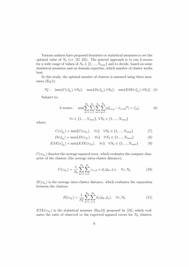
Figure 1 illustrates the developed algorithm for selecting the typical periods.
11
Chapter 5. Selection of typical operating periods
constraints with an upper limit of �aj . The auxiliary model of Eq.5.12 is expressed as Eq. 5.22:
minµk ,zi ,k
{Nk} (5.22)
Subject to:
k-means : min��Nk
k=1
�Nii=1 d(µk , xi )� zi ,k
�
�apr o f i l e,Nk
� �a1 �a
�acdc,Nk
� �a2 �a
ELDC aNk
� �a3 �a
�aLDC ,Nk
� �a4 �a
�apr od ,�,Nk
� �a5 �a
Figure 5.2 shows the developed algorithm for selecting typical periods. The algorithm proceedsas follows:
• Step 1: Break down the energy profile into Ni observations made up of Na attributeswith Ng (a) values.
xi ,a,g 1 � i � Ni 1 � a � Na 1 � g � Ng (a) (5.23)
• Step 2: Set constraints on the maximum allowable values of the performance indicators(�a
j ) and apply k-means algorithm for selecting N�k periods. This step should be repeated
with several random starting points as long as the constraints are not met. If this stepdoes not converge into a feasible solution after Vmax iterations (i.e. Vmax = 1000), itimplies that the constraints set on the performance indicators are too constraining andthey should either be relaxed by the user or the number of typical periods should beincreased. Finally the result will be µ�
k typical periods.
• Step 3: If the optimal number of periods, N�k , and the indicators’ threshold, �a
j , arenot known, run k-means for values of Nk � {1, ..., Nmax }, with v � {1, ...,Vmax } randomstarting points (i.e. Vmax = 1000, Nmax = 20). The k-means clustering is very quick andrunning it with 1000 random initial points is a matter of minutes.
• Step 4: Calculate values of performance indicators, expected squared error (ESE vNk
),average intra-clusters distance (C v (Nk )) and average inter-clusters distance (Dv (Nk ))for Nk � {1, ..., Nmax } and v � {1, ...,Vmax} iterations.
• Step 5: Draw the Pareto frontier of each performance indicator and select the minimumaccepted number of clusters N �
k , for which the indicators’ improvement on the Paretofrontier from N �
k to N �k +1 is less than 20% (Eq.5.24). This implies that by increasing
62
1" !!,!,! !!!!,!,! ! !!! !!"#!!!∗ !are$known?$
yes$
2"
Generate"N*#typical""periods"
S.T:$$$$k&means$clustering$P(j)<=$$$
K%means#clustering"
Converge?$$
yes$
No$
New$star>ng$point$v=v+1$
V$<=$Vmax?$yes$
No$
Increase$!!! !!"!!!∗ !
v=1$
K%means#clustering"
No$
Run$k&means$several$>mes$for$!! ∈ 1,… ,!!"# !!"#ℎ!! ∈ {1,… , !!"#}!!
Calculate$values$of$performance$indicators,$$ESEv(Nk),$Cv(Nk)$and$Dv(Nk)$for$
Draw$the$Pareto$fron>er$of$each$performance$indicator$and$select$$$$$$,$the$minimum$accepted$
number$of$clusters$
3"
4"
5"
Select$the$op>mal$typical$periods,$$$$$$$,$in$which;$6"!!∗ !≥ !!! !!"#!!
! !!∗ = min
2 4 6 8 10 12 14 16 18 20 22 2451
51.5
52
52.5
53
53.5
54
54.5
55
55.5
56
Hour of day
Ener
gy d
eman
d pr
ofile
[MW
]Sequential segmented typical day
Typical day profileSegmented hour 1Segmented hour 2Segmented hour 3Segmented hour 4Segmented hour 5
Figure 2: Segmented typical periods
Extreme values are then forced into the segments. Therefore, the endresult is the segmented typical periods (h
k,a,N
s
⇤k
+1), made up of N⇤k
typical
periods with Ns
⇤k
+ 1 segments.The performance indicator, which is here the maximum tolerated di↵er-
ence in the total demand during each period (�a
sum,k,N
s
k
), is expressed as
follows (Eq.29):
�a
sum,k,N
s
k
=|P
N
g
g=1 µ⇤k,a,g
�P
N
s
k
s
k
=1 dk,sk
⇥ hk,a,s
k
|P
N
g
g=1 µ⇤k,a,g
8a, k 2 {1, ..., N⇤k
} (29)
dk,s
k
represents the duration (number of time step) of each segment, andhk,a,s
k
refers to the value of segment sk
in typical day k for attribute a (seg-mented typical periods).
If the best number of segments (Ns
⇤k
) and the indicator’s threshold (�a
sum,k,N
s
k
)are not known, the following steps are proposed to optimize the segmentedtypical periods;
• Step 1: Run k-means for values ofNs
k
2 {1, ..., Ng
}, with v0 2 {1, ..., V 0max
}random starting points and calculate �a
sum,k,N
s
k
for each starting point.
13

• Step 2: Draw the Pareto frontier of �a
sum,k,N
s
k
and select the minimumaccepted number of segmentsN
s
0k
, for which the indicator’ improvementon the Pareto frontier from N
s
0k
to Ns
0k
+ 1 is less than 20% (Eq.30).
minNs
0k
, 8k (30)
Where:
|�a
sum,k,N
s
0k
��a
sum,k,N
s
0k
+1
�a
sum,k,N
s
0k
| 6 0.2 8a, k
• Step 3: Select the best segmented typical period taking into accountN
s
0k
(Ns
⇤k
> Ns
0k
) selected in step 2, the ESE, inter and intra clustersdistances (Section 2.1.1).
• Step 4: Once segmented typical periods have been selected, extremevalues are then forced into the segments, thereby adding one moresegment to the segmented typical periods
• Step 5: Repeat steps 1 to 4 for 8k 2 {2, ..., N⇤k
} to calculate the seg-ments of each typical period k.
The results of the algorithm may not always converge to the desired sequen-tial segments. In order to reach sequential time steps, the proposed algorithmcan be modified by considering the method developed by Balachandra andChandru [8].
3. Illustrative examples
Two test cases are discussed to demonstrate the proposed method. Thefirst case is a full-scale problem with a 23 years time horizon for supplyingthe heating demand of a district. The second case study aims to illustratethe proposed method by considering four type of attributes; the hourly solarirradiation, the electricity price, the heating and electricity demand profilesof a small district.
3.1. Test case 1
The multi-period MINLP optimization model is investigated in [1] inorder to optimize the design and the operating strategy of district energy
14

systems. The developed model is decomposed into a master and a slave op-timizations. The master nonlinear model optimizes the system configurationand the size of conversion technologies. Meanwhile, the slave multi-periodmixed integer linear model calculates the best operating schedule of selectedconversion technologies.
The test case presented in [1] is used to illustrate the application of thetypical periods selection method. The goal is to optimize the operating strat-egy of the fixed system configuration, in such a way as to supply the heatingrequirement of the urban area with optimal operating costs. The averageannual heat demand is equal to 2100 GWh. In order to do so the slavemulti-period MILP optimization model is applied [1]. The available conver-sion technologies are an incinerator with 160 MW
th
, a 100 MWth
biomassboiler and a 130 MW
th
coal boiler. In addition a natural gas boiler has to besized to supply the peak loads. All units are assumed to be able to operateat any time with no limit on the availability of resources (Table 1).
Table 1: CO2 intensity and price of available resources
Resources 4CO2: Price: [25][kg/MJ ] [e/MJ ]:
Electricity 0.3071 [26] 0.0198Natural Gas 0.0641 0.0105Coal 0.0852 0.0030Biomass 0 0.0036
The operating schedule of the system will be optimized by consideringthe di↵erent type of typical periods. In order to validate and demonstratethe proposed typical period selection method, the optimization results willbe compared with a reference case (Section 3.1.4).
In the present work the hourly heating demand profile is estimated usingmeteorological data and the heating signature [27]. The heating signatureis a linear model of the thermal power requirements as a function of theambient temperature [27].
The ambient temperatures of the last 23 years from 1990 to 2012 areconsidered to estimate the hourly heating demand profile of the district (Fig-ure 3) [27]. The first 20 years with 175200 (20 ⇥ 8760) time steps are usedto select the typical periods, and the last 3 years data, from 2010 to 2012,are used for validation.
15

Form these data, a mean typical year with 8760 time steps is defined byconsidering the average values over 20 years (Figure 3).
2 4 6 8 10 12 14 16x 104
100
200
300
400
500
Heat
dem
and
[MW
]
Heat demand & Outdoor temperature: 20 years
HDP
2 4 6 8 10 12 14 16x 104
0
20
40
Hours
Out
door
tem
pera
ture
Outdoor temperature
1000 2000 3000 4000 5000 6000 7000 8000100
200
300
400
Hours
Heat
dem
and
[MW
] Heat demand & Outdoor temperature: a typical year
HDP
1000 2000 3000 4000 5000 6000 7000 80000
10
20
30
Hours
Out
door
tem
pera
ture
outdoor temperature
Figure 3: The ambient temperatures and estimated heat demands: 20 years andthe mean typical year.
In order to reduce the optimization size, the heating demand data (seriesof 175200 values) is compressed to a limited number of typical periods byapplying the following methods;
1. Empirical method: 13 typical periods, one per month as the averagevalues and one extreme day [7].
2. Proposed k-means clustering method using the mean typical year data.
3. Proposed k-means clustering method using the original 20 years dataequivalent to the lifetime of equipment.
3.1.1. Empirical periods
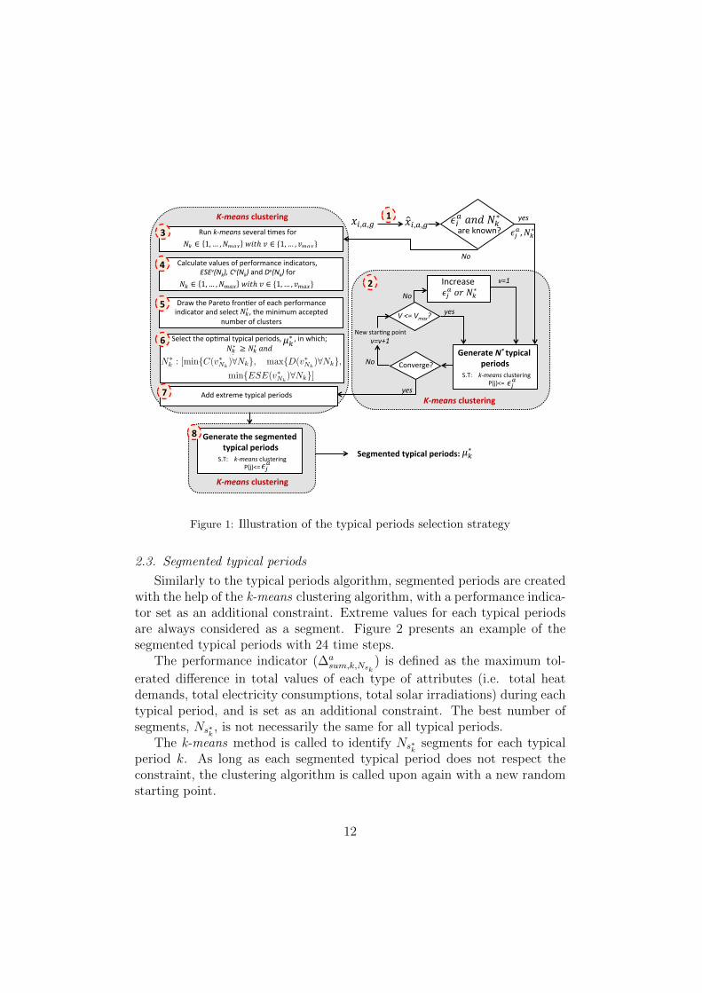
Figure 4 refers to the mean typical year with Ni
= 365 observations,heating demand as an attribute (N
a
= 1), 24 values for each observation(N
g
= 24), and selected empirical periods with 312 (13⇥24) total time steps.
The five performance indicators proposed in Section 2.2 are used to cal-culate the qualities of the empirical periods for representing the original 20years data as well as the mean typical year (Table 2). The e↵ects of theempirical periods accuracy on the optimization results will be studied inSection 3.1.4.
16
1000 2000 3000 4000 5000 6000 7000 80000
100
200
300
400
Hea
t Dem
and
Prof
ile [M
W]
0 1000 2000 3000 4000 5000 6000 7000 80000
50
100
150
200
250
300
350
400
A typical year [hour]
Load
Dur
atio
n C
urve
[MW
]
HDPday 1day 2day 3day 4day 5day 6day 7day 8day 9day 10day 11day 12day 13
Figure 4: The empirical typical periods and the mean typical year heatingdemand.
Table 2: The qualities of the empirical periods compare to the original 20 yearsdata, as well as the mean typical year data.
Quality The empirical periods and The empirical periods and
indicators the mean typical year data the original 20 years data
�cdc
0.071 0.173�profile
0.059 0.117ELDC 0.056 0.153�
LDC
0 0�
prod,0.07 113 4983
3.1.2. Proposed k-means clustering approach using the mean typical year data
In order to select the best representative typical periods from the meantypical year data, the proposed method in Section 2.2 is applied by consid-ering N
k
2 {1, ..., 15} and Vmax
= 1000 random starting points.According to Eq.5 and Eq.26, the best number of typical periods is chosen
by considering the values of the intra and inter clusters distances, ESE andthe Pareto frontiers of the five performance indicators (Figures 5 and 6).
Figure 5 indicates that forNk
> 5 the values of the performance indicators
17

become constant and the relative di↵erences between Nk
and Nk
+1 are lessthan 0.2. The relative di↵erences become close to zero by increasing thenumber of periods to N
k
= 15. However, this leads to an increased size ofthe optimization model. A compromise between the optimization size and thequality of the typical periods is necessary. Therefore, the minimum acceptednumber of clusters is equal to 5 (N 0
k
= 5). The highest values of the averageinter-clusters distance are obtained by N
k
= 6 and 15 periods (Figure 6). Thelowest ESE values are obtained for N
k
= 2, Nk
= 6 and Nk
= 14 periods,and for more than 6 clusters the average intra-clusters distance tends towardszero (Figure 6). As a result, 6 periods plus one extreme period, are chosenas the best and qualified number of the typical periods (N⇤
k
= 7).We go further by breaking up the 24 time steps of each representative pe-
riod into smaller segments. The algorithm proposed in Section 2.3 is applied.The results indicate the optimal number of segments for the selected typicalperiods is equal to N
s
⇤k
= 5 for 8k 2 {2, ..., 7} and Ns
⇤k
= 4 segments for thesummer period (k = 1). Figure 7 illustrates how the mean typical year canbe split up into its respective 7 typical periods with total 34 (6⇥ 5+ 4) timesteps. The 5-44% improvements of the quality of the 7 typical periods (seesupplementary Table S1 and Table S2), with respect to the load deviationand variances, illustrates the advantages of the proposed k-means clusteringmethod.
2 4 6 8 10 12 14 150
0.1
0.3
0.5
0.7
0.9
1
Number of typical periods
Performance Indicators Pareto Frontiers
�cdc�profile
ELDC�LDC
2 4 6 8 10 12 140
0.1
0.2
0.3
0.4
0.5
0.6
0.7
0.8
0.9
1
Number of typical periods
Rel
ativ
e di
ffere
nces
Relative differences between Nk and Nk+1
�cdc
�profile
ELDC�LDC
Figure 5: Pareto frontiers of typical periods’ normalized performance indicatorsusing the mean typical year data: Case study 1.
18

0 2 4 6 8 10 12 14 16
0
1
2
3
4
5
6
7
8
9
10x 106
Number of clusters (Nk)
Ave
rage
intr
a−cl
uste
rs d
ista
nce
(C* (N
k))
0 2 4 6 8 10 12 14 160
0.5
1
1.5
2
2.5
3
3.5
4
4.5x 10⁵
Number of clusters (Nk)
Ave
rage
inte
r−cl
uste
rs d
ista
nce
(D* (N
k)
0 2 4 6 8 10 12 14 160
0.2
0.4
0.6
0.8
1
1.2
1.4
Number of clusters (Nk)
ESE* (N
k)
Figure 6: Intra and inter clusters distances and ESE measures as a function of thenumber of typical periods using the mean typical year data: Case study 1.
19

1000 2000 3000 4000 5000 6000 7000 80000
100
200
300
400
Hour [h]
Hea
t Dem
and
Prof
ile [M
W] HDP and LDC for Segmented Typical Days
0 1000 2000 3000 4000 5000 6000 7000 80000
100
200
300
400
Hour [h]
Load
Dur
atio
n C
urve
[MW
]
HDPTypical day 1Typical day 2Typical day 3Typical day 4Typical day 5Typical day 6Typical day 7
Figure 7: The mean typical year heat demand profile with 7 typical periods andcorresponding 34 total time steps.
20

3.1.3. Proposed k-means clustering method using the 20 years data
Here, instead of the mean typical year, the heating requirements over 20years (Figure 3) are used to select typical periods. Table 3 presents the valuesof the performance indicators for di↵erent number of typical periods from 5to 13. The quality of the typical periods are improved by increasing N
k
.However, the relative improvement for N 0 > 5 is less than 20%. Followingthe proposed method, the optimal number of typical periods, N⇤
k
= 7, wasassessed using; Pareto frontiers of performance indicators, inter and intracluster distances and ESE.
In Table 4 the column ”Deviation” compares the quality of N⇤k
=7 typicalperiods with corresponding 34 time steps (supplementary Figure S1) andthe empirical periods with 312 (13 ⇥ 24) time steps (Figure 4). The fiveindicators present 8-63% higher qualities for N⇤
k
= 7, indicating that theproposed k-means clustering method provides the better approximation ofthe original data.
The qualities of the mean typical year for representing the original 20years data are summarized in Table 3. Even though the classic mean typicalyear contains 8760 time steps, the qualities of the 7 typical periods are 35-60% higher (supplementary Table S3).
Table 3: The quality indicators of the typical periods using the original 20 years data
No. periods Nk
=5 N⇤k
=7 Nk
=9 Nk
=11 Nk
=13 The mean typical yearNo.time steps 24 34 44 54 64 365 ⇥24
�cdc
0.096 0.063 0.062 0.058 0.050 0.157�profile
0.115 0.108 0.100 0.098 0.096 0.102ELDC 0.109 0.092 0.087 0.085 0.082 0.141�
LDC
0 0 0 0 0 0.282�
prod,0.07 4191 2128 2044 1666 1200 4582
3.1.4. Validation and verification
The illustrative example is studied in order to identify the ability of thetypical periods methodology for identifing an optimal operating strategy ofthe energy system. The typical periods selected using 1990 to 2009 data isapplied on a period from 2010 to 2012 (a validation period) and comparedto an accurate reference case. The total fuel consumption and the size of thepeak boiler are considered as indicators to compare the results.
21
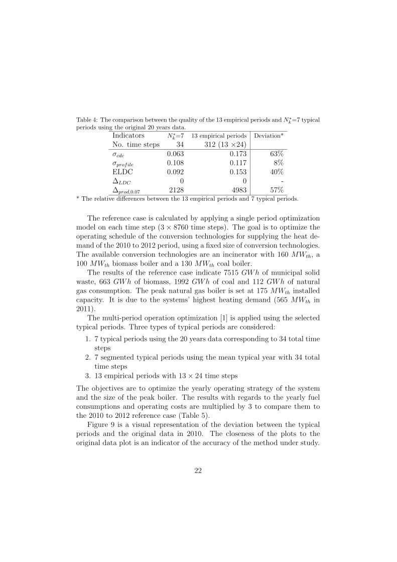
Table 4: The comparison between the quality of the 13 empirical periods and N⇤k=7 typical
periods using the original 20 years data.
Indicators N⇤k=7 13 empirical periods Deviation*
No. time steps 34 312 (13 ⇥24)�cdc
0.063 0.173 63%�profile
0.108 0.117 8%ELDC 0.092 0.153 40%�
LDC
0 0 -�
prod,0.07 2128 4983 57%* The relative di↵erences between the 13 empirical periods and 7 typical periods.
The reference case is calculated by applying a single period optimizationmodel on each time step (3 ⇥ 8760 time steps). The goal is to optimize theoperating schedule of the conversion technologies for supplying the heat de-mand of the 2010 to 2012 period, using a fixed size of conversion technologies.The available conversion technologies are an incinerator with 160 MW
th
, a100 MW
th
biomass boiler and a 130 MWth
coal boiler.The results of the reference case indicate 7515 GWh of municipal solid
waste, 663 GWh of biomass, 1992 GWh of coal and 112 GWh of naturalgas consumption. The peak natural gas boiler is set at 175 MW
th
installedcapacity. It is due to the systems’ highest heating demand (565 MW
th
in2011).
The multi-period operation optimization [1] is applied using the selectedtypical periods. Three types of typical periods are considered:
1. 7 typical periods using the 20 years data corresponding to 34 total timesteps
2. 7 segmented typical periods using the mean typical year with 34 totaltime steps
3. 13 empirical periods with 13⇥ 24 time steps
The objectives are to optimize the yearly operating strategy of the systemand the size of the peak boiler. The results with regards to the yearly fuelconsumptions and operating costs are multiplied by 3 to compare them tothe 2010 to 2012 reference case (Table 5).
Figure 9 is a visual representation of the deviation between the typicalperiods and the original data in 2010. The closeness of the plots to theoriginal data plot is an indicator of the accuracy of the method under study.
22
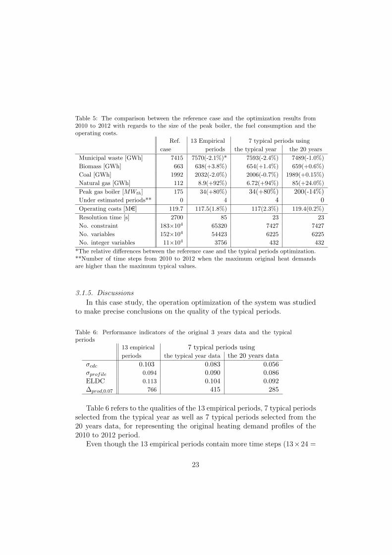
Table 5: The comparison between the reference case and the optimization results from2010 to 2012 with regards to the size of the peak boiler, the fuel consumption and theoperating costs.
Ref. 13 Empirical 7 typical periods using
case periods the typical year the 20 years
Municipal waste [GWh] 7415 7570(-2.1%)* 7593(-2.4%) 7489(-1.0%)
Biomass [GWh] 663 638(+3.8%) 654(+1.4%) 659(+0.6%)
Coal [GWh] 1992 2032(-2.0%) 2006(-0.7%) 1989(+0.15%)
Natural gas [GWh] 112 8.9(+92%) 6.72(+94%) 85(+24.0%)
Peak gas boiler [MWth] 175 34(+80%) 34(+80%) 200(-14%)Under estimated periods** 0 4 4 0
Operating costs [Me] 119.7 117.5(1.8%) 117(2.3%) 119.4(0.2%)
Resolution time [s] 2700 85 23 23
No. constraint 183⇥104 65320 7427 7427
No. variables 152⇥104 54423 6225 6225
No. integer variables 11⇥104 3756 432 432
*The relative di↵erences between the reference case and the typical periods optimization.**Number of time steps from 2010 to 2012 when the maximum original heat demandsare higher than the maximum typical values.
3.1.5. Discussions
In this case study, the operation optimization of the system was studiedto make precise conclusions on the quality of the typical periods.
Table 6: Performance indicators of the original 3 years data and the typicalperiods
13 empirical 7 typical periods usingperiods the typical year data the 20 years data
�cdc
0.103 0.083 0.056�profile
0.094 0.090 0.086ELDC 0.113 0.104 0.092�
prod,0.07 766 415 285
Table 6 refers to the qualities of the 13 empirical periods, 7 typical periodsselected from the typical year as well as 7 typical periods selected from the20 years data, for representing the original heating demand profiles of the2010 to 2012 period.
Even though the 13 empirical periods contain more time steps (13⇥24 =
23

150 200 250 300 350 400 450
150
200
250
300
350
400
450
Sorted typical days values
Sorte
d or
igin
al d
ata
A typical year heat load [MW]
Original data7 segmented typical days 7 typical days
Sorted original hourly heat demand profile in 2010 [MW]
Sor
ted
typi
cal p
erio
ds h
eat d
eman
d [M
W]
Figure 8: The sorted values of the original heat demand profile in 2010 versus thesorted heat demand profiles of 7 typical periods with 7⇥24 time steps and 7 typicalperiods with 34 (6 ⇥ 5 + 4) total time steps resulting from the mean typical yeardata. This figure illustrates the deviation between the original heat loads and thetypical periods
312), the qualities of the results, with respect to the heat load deviation andvariances, are higher with 7 typical periods. The 7 typical periods selectedfrom the original 20 years data presented the most accurate results (Table 6).
With respect to the size of the peak boiler, it was underestimated by boththe empirical periods and the 7 periods selected from the mean typical year.The obtained size was 80% less than that found by the reference case. Thisis explained by the extreme period of 2011, with -10 oC ambient temperatureand 565 MW
th
heat load demand not being represented in the mean typicalyear. The frequency of such a high demand is only 4 periods over 3 years(Table 5), which is not significant. In the optimization with the 7 typicalperiods selected using the original 20 years data, the peak boiler capacity is14% higher compared to the reference case. This is because the heat load ofthe extreme periods during the first 20 years is 590 MW
th
, which is not thecase from 2010 to 2012.
With respect to the total fuel consumption and operating costs, the rel-
24

ative di↵erences between the reference case and 7 typical periods selectedfrom 20 years’ heat loads present the least error, especially for biomass andnatural gas consumption (Table 5).
We can sum up that 7 typical periods selected using the 20 years datagive an accurate picture of the system’s operations.
The optimization and reference case resolution times are summarized inTable 5. The results pointed out that the resolution time increases signifi-cantly with respect to the time steps of the demand profiles. The optimiza-tion may reach more accurate results by extending the number of time steps.With increased accuracy comes increased computational costs, with associ-ated memory problems and prohibitive resolution time. This is especiallytrue for solving multi-objective optimizations with a MINLP model. A com-promise should always be made between the resolution time and the numberof time steps.
3.2. Test case 2
The second test case is proposed to illustrate the application of the typicalperiods to the heating demand, electricity demand, electricity price (eex.com)and solar irradiation data of a district with 30,000 inhabitants. The aim isto optimize the operating strategy of the fixed system configuration, in sucha way as to supply the energy requirement of the urban area with optimaloperating costs. The data of the last 4 years from 2009 to 2012 are available.The first 3 years are used to select the typical periods and the last year, 2012,is used to validate the selected typical periods. The period is defined as aday with 24 time steps.
The case comprises 5 conversion technologies (Figure 9); a 4 MWel
gasturbine, a 6 MW
el
gas engine, a 30 MWth
biomass boiler, a 35 MWth
gasboiler and 50,000 m2 of solar thermal, using economic data from [28]. A41 MW
th
peak natural gas boiler is sized for the systems highest demand,present on the extreme day (120 MW heating demand). The possibility alsoexists to import electricity from the main grid. The solar thermal plant re-quires accurate meteorological data to determine the capacity of this technol-ogy for each given period, reason for which the solar irradiation and ambienttemperatures profiles are also included into the study.
Following the proposed algorithm in section 2.2, for Nk
> 6 the values ofperformance indicators become constant and the relative di↵erences betweenN
k
and Nk
+1 are close to zero (see supplementary Figure S2). This indicatesthat by increasing the number of clusters from N
k
to Nk
+1 the improvement
25

Gas$Engine$6$[MWel]$
Gas$$Boiler$35$[MW]$
Biomass$boiler$30$[MW]$
Fuel$
District$hea>ng$networks$
Electrical$grid$
Electricity$
" =40$⁰C$
" =60$⁰C$
Gas$Turbine$4$[MWel]$
Figure 9: Test case 2 - an urban area with 30,000 inhabitants
of the typical periods quality is not significant. As a result, the minimumaccepted number of clusters is equal to 6 (N 0
k
= 6). Based on the values of thethree statistical measures for N
k
ranging from 1 to 15 (supplementary FigureS3) and according to Eq.14, N
k
= 7 has the lowest value for the average intra-clusters distance, the highest value for the average inter-clusters distance andthe lowest value for ESE measure.
While electricity can be imported from the main grid, the central plantmust supply all heating requirements, especially in the extreme period withthe maximum heat demand. Therefore, the extreme period with the highestheat demand is added. To resume, 7 periods plus one extreme period arechosen as an optimal number of typical periods (N⇤
k
= 8).We go further by breaking up the time steps of each representative period
into 5 smaller segments (Section 2.3). Figure 10 presents the original datain 2012 and respective 8 typical periods with total 40 (8 ⇥ 5) time steps.
In order to make a precise conclusion on the quality of the typical periods,the reference case of 2012 were compared with the typical periods operationoptimization results in terms of the operating cost, fuel consumption and theheat production of each equipment (Table 7). We investigate the 8 typicalperiods with 40 time steps, as well as 8 typical periods with total 192 (8⇥24)
26

time steps.With respect to the heat share and operating costs, the 8 typical periods
with 192 (8⇥ 24) time steps led to the most accurate results, as the relativeerror with the reference case shows. A period with the maximum heat de-mand is presented by all three type of typical periods. However, the totalnumber of operating hours of the 41 MW
th
peak boiler in 2012 is 36-59%under estimated by the typical periods (59% by the empirical periods, 36%by 8 typical periods with 192 time steps, and 52% by 8 typical periods with35 time steps). Therefore, 28-53% errors in the peak boiler’s heat productionare pointed out in Table 7.
Apart from the peak boiler, the maximum relative di↵erences between theoptimization results of 8 typical periods with 40 time steps and the results of8 typical periods with 8⇥24 time steps is only 2.2%. However, its resolutiontime is 60% less. The optimization may reach more accurate results byextending the number of time steps but this will increase the computationalcosts.
Table 7: Test case 2 - Comparison between the reference case and the typical periodsoptimization results in terms of the operating costs and the heat production
Reference Empirical periods 8 periods 8 periods
No. time steps 365⇥24 13⇥24 8⇥24 8⇥5
Solar thermal [GWh] 22.7 25.9 (-14.1%)* 23 (-1.3%)* 23.4 (-3.1%)
Biomass boiler [GWh] 134.8 141.0 (-4.6%) 136.5 (-1.3%) 136.5 (-1.3%)
Gas boiler [GWh] 48.3 36.7 (+24.1%) 46.6 (+3.5%) 46.3 (+4.1%)
Peak boiler [GWh] 3.2 1.5 (+53%) 2.3 (+28%) 1.7 (+46.7%)
Gas engine [GWh] 43.5 48.6 (-11.7%) 44.1 (-1.4%) 45.1 (-3.7%)
Gas turbine [GWh] 37.2 39.6 (-6.4%) 37.8 (-1.6%) 37.8 (-1.6%)
Electricity import [GWh] 57.9 52.0 (+10.2%) 57.1 (+1.4%) 56.2 (+2.9%)
Natural gas fuel [GWh] 232.1 232.8 (-0.3 %) 231.4 (+0.3 %) 232.8 (-0.3 %)
Biomass fuel [GWh] 170 178.5 (-5%) 173 (-1.8%) 173 (-1.8%)
Resolution time [s] 760 64 48 19
Operating costs [Me] 13.9 13.7 (+1.4%) 13.8 (+0.7%) 13.8 (+0.7%)
*The relative di↵erences between the reference case and the typical periods optimizationresults
27

1,000 2000 3,000 4,000 5,000 6,000 7,000 8,0000
50
100
Heat
pro
file
[MW
]
Heat load with 8 segmented sequential typical days
1000 2000 3000 4000 5000 6000 7000 800005
10152025
Elec
trici
ty
prof
ile [M
W] Electricity deamnd with 8 segmented sequential typical days
1000 2000 3000 4000 5000 6000 7000 80000
50
100
Elec
trici
ty p
rice
[Eur
o/M
Wh] Electricity price with 8 segmented sequential typical days
1000 2000 3000 4000 5000 6000 7000 80000
200400600800
HoursSola
r irr
adia
tion
[W/m
2 ]
Solar irradiation with 8 segmented sequential typical days
Original profileDay 1Day 2Day 3Day 4Day 5Day 6Day 7Day 8
Figure 10: Test case 2- The heat and the electricity demand profiles and the solarirradiation with 8 typical periods and 40 time steps in 2012
28

4. Conclusions
In the present work, a new method has been developed to select the typ-ical periods from the multiple time-varying demand profiles. The proposedmethod is based on the k-means clustering algorithm. It is developed byconsidering five performance indicators as additional constraints to guaran-tee reaching a qualified local optimal. In addition, three statistical measuresare used for selecting the optimal number of typical periods.
We go further by breaking up the time steps of each representative periodinto smaller number of segments, further reducing the problem complexity,while respecting significant characteristics such as the peak demands andprofile trends. The proposed method can easily be modified to work withtypical weeks and also to accommodate other considerations such as a com-plex electric tari↵ structure or maintenance periods.
Two test cases are discussed to demonstrate the proposed method. Theresults of the first test case illustrate that the whole lifetime of conversiontechnologies can be considered for selecting the typical periods, and the pro-posed method can reduce a complete demand data with 20⇥8760 time stepsinto 7 segmented typical periods with total 34 time steps. The second testcase illustrates the advantages of the proposed method for selecting the typ-ical periods with respect to several attributes such as the hourly heatingprofile, the solar irradiation, the electricity demand and the ambient temper-ature.
29

Nomenclature
MILP mixed integer linear programming
C(vN
k
) the average intra-clusters distance
D(vN
k
) the average inter-clusters distance
xi,a,g
observation i with attribute a and measurement g
zi,k
a binary variable equal to 1 if observation i placed in the typicalperiod k
xi,a
the average value of observation i with attribute a
µk,a,g
the centre of the cluster k
µk,a
the average value of the typical period k
Nk
the number of the typical periods
N⇤k
the optimal number of the typical periods
Ns
⇤k
the best number of segment for the typical period k
d(xi
, µk
) the distance between observation i and the center of the cluster
Ni
the number of the observation
Na
the number of attributes
v the index for the random starting points
Vmax
the maximum number of random starting points
Ng
the number of measurements
LDCa
o
the load duration curve of the original data of attribute a
LDCa
e
the load duration curve of typical periods of attribute a
�a
profile
the profile deviation of attribute a
�a
cdc
the deviation from the load duration curve of the average values ofeach period and attribute a
ELDCa the error in load duration curve deviation of attribute a
�a
LDC
the maximum load duration curve deviation of attribute a
�a
prod,�,N
k
Number of periods whose relative error is higher than �
⇠ threshold for performance indicators’ improvement
30
�a
sum,k,N
s
k
the maximum tolerated di↵erence in total values of attribute a intypical period k for N
s
k
number of segment
hk,a,s
k
the value of segment sk
in typical period k corresponding to attributea
dk,s
k
the duration (number of time step) in segment sk
References
[1] S. Fazlollahi, F. Marechal, Multi-objective, multi-period optimizationof biomass conversion technologies using evolutionary algorithms andmixed integer linear programming (MILP), Applied Thermal Engineer-ing 50 (2013) 1504 - 1513.
[2] R. P.Menon, M. Paolone, F. Marechal, Study of optimal design of poly-generation systems in optimal control strategies, Energy 55 (2013) 134- 141.
[3] F. Marechal, B. Kalitventze↵, Targeting the integration of multi-periodutility systems for site scale process integration, Applied Thermal En-gineering 23 (2003) 1763 - 1784.
[4] J. Ortiga, J. Bruno, A. Coronas, Selection of typical days for the char-acterisation of energy demand in cogeneration and trigeneration opti-misation models for buildings, Energy Conversion and Management 52(2011) 1934 - 1942.
[5] M. A. Lozano, J. C. Ramos, M. Carvalho, L. M. Serra, Structure opti-mization of energy supply systems in tertiary sector buildings, Energyand Buildings 41 (2009) 1063 - 1075.
[6] M. Casisi, P. Pinamonti, M. Reini, Optimal lay-out and operation ofcombined heat & power (CHP) distributed generation systems, Energy34 (2009) 2175 - 2183.
[7] G. Mavrotas, D. Diakoulaki, K. Florios, P. Georgiou, A mathematicalprogramming framework for energy planning in services’ sector buildingsunder uncertainty in load demand: The case of a hospital in Athens,Energy Policy 36 (2008) 2415 - 2429.
31

[8] P. Balachandra, V. Chandru, Modelling electricity demand with repre-sentative load curves, Energy 24 (1999) 219 - 230.
[9] F. Domnguez-Muoz, J. M. Cejudo-Lpez, A. Carrillo-Andrs, M. Gallardo-Salazar, Selection of typical demand days for CHP optimization, Energyand Buildings 43 (2011) 3036 - 3043.
[10] G.A.F Seber, Multivariate observations, New York: John Wiley & Sons,(1984).
[11] C.H. Marton, A. Elkamel, T.A. Duever, An order-specific clusteringalgorithm for the determination of representative demand curves, Com-puter and Chemical Engineering 32 (1999) 1373 - 1380.
[12] R.E. Steuer, Multiple criteria optimization: theory computation andapplication, Robert E. Krieger Publishing Malabar (Florida) (1989) .
[13] S. Fazlollahi, P. Mandel, G. Becker, F. Marechal, Methods for multi-objective investment and operating optimization of complex energy sys-tems, Energy 45 (2012) 12 - 22.
[14] A. K. Jain, M. N. Murty, P. J. Flynn, Data clustering: A review, ACMComputing Surveys 31 (1999) 264 – 323.
[15] G. Gan, C. Ma, J. Wu, Data clustering: Theory, algorithms, and ap-plications, ASA-SIAM Series on Statistics and Applied Mathematics(2007).
[16] A. K. Jain, R. C. Dubes, Algorithms for clustering data, Prentice HallCollege Div (1988).
[17] H. Steinhaus, Sur la division des corp materiels en parties, Bull. Acad.Polon. Sci 1 (1956) 801 – 804.
[18] G. H. Ball, D. J. Hall, Isodata, a novel method of data analysis andpattern classification, Stanford Research Institute (1965).
[19] J. B. MacQueen, Some methods for classification and analysis of multi-variate observations, Fifth Berkeley symposium on mathematics, statis-tics and probability, University of California Press (1966) 281297.
32

[20] A. K. Jain, Data clustering: 50 years beyond k-means, Pattern Recog-nition Letters 31 (2010) 651–666.
[21] R. Kothari, D. Pitts, On finding the number of clusters, Pattern Recog-nition Letters 20 (1999) 405–416.
[22] S. Ray, R. H. Turi, Determination of number of clusters in k-meansclustering and application in colour image segmentation, in Proceedingsof the Fourth International Conference on Advances in Pattern Recog-nition and Digital Techniques (1999).
[23] R. Tibshirani, G. Walther, T. Hastie, On finding the number of clusters,Journal of the Royal Statistical Society (2001) 411–423.
[24] D. T. Pham, S. S. Dimov, C. D. Nguyen, Selection of k in k-meansclustering, Mechanical Engineering Science 219 (2004) 103–119.
[25] IEA, Energy statistics 2011, relation with member countries poland,international energy agency (2011). Viewed 13 January.
[26] IPCC, Intergovernmental panel on climate change, IPCC Fourth As-sessment Report, The Physical Science Basis, Geneva, CH, Switzerland(2007).
[27] L. Girardin, F. Marechal, M. Dubuis, N. Calame-Darbellay, D. Favrat,Energis: A geographical information based system for the evaluation ofintegrated energy conversion systems in urban areas, Energy 35 (2010)830 – 840.
[28] L. Gerber, Integration of Life Cycle Assessment in the conceptual designof renewable energy conversion systems, Ph.D. thesis, Ecole Polytech-nique Federale de Lausanne, Switzerland, 2013.
Acknowledgments: The authors would like to acknowledge Veolia Envi-ronnement Recherche et Innovation (VERI) for the financial support.
33