multi-particle azimuthal correlations for extracting event
TRANSCRIPT
Abilene Christian University Abilene Christian University
Digital Commons @ ACU Digital Commons @ ACU
Engineering and Physics College of Arts and Sciences
2019
Multi-particle azimuthal correlations for extracting event-by-event Multi-particle azimuthal correlations for extracting event-by-event
elliptic and triangular flow in Au+Au collisions at √sNN = 200 GeV elliptic and triangular flow in Au+Au collisions at sNN = 200 GeV
Mike Daugherity Abilene Christian University, [email protected]
Donald Isenhower Abilene Christian University, [email protected]
Rusty Towell Abilene Christian University, [email protected]
Follow this and additional works at: https://digitalcommons.acu.edu/engineer_physics
Recommended Citation Recommended Citation Daugherity, Mike; Isenhower, Donald; and Towell, Rusty, "Multi-particle azimuthal correlations for extracting event-by-event elliptic and triangular flow in Au+Au collisions at √sNN = 200 GeV" (2019). Engineering and Physics. 12. https://digitalcommons.acu.edu/engineer_physics/12
This Article is brought to you for free and open access by the College of Arts and Sciences at Digital Commons @ ACU. It has been accepted for inclusion in Engineering and Physics by an authorized administrator of Digital Commons @ ACU.
Multi-particle azimuthal correlations for extracting event-by-event elliptic andtriangular flow in Au+Au collisions at
√sNN
= 200 GeV
A. Adare,13 C. Aidala,41 N.N. Ajitanand,58, ∗ Y. Akiba,53, 54, † M. Alfred,23 N. Apadula,28, 59 H. Asano,34, 53
B. Azmoun,7 V. Babintsev,24 A. Bagoly,17 M. Bai,6 N.S. Bandara,40 B. Bannier,59 K.N. Barish,8 S. Bathe,5, 54
A. Bazilevsky,7 M. Beaumier,8 S. Beckman,13 R. Belmont,13, 41, 47 A. Berdnikov,56 Y. Berdnikov,56 D.S. Blau,33, 44
M. Boer,36 J.S. Bok,46 K. Boyle,54 M.L. Brooks,36 J. Bryslawskyj,5, 8 V. Bumazhnov,24 S. Campbell,14, 28
V. Canoa Roman,59 C.-H. Chen,54 C.Y. Chi,14 M. Chiu,7 I.J. Choi,25 J.B. Choi,10, ∗ T. Chujo,62 Z. Citron,64
M. Connors,21, 54 M. Csanad,17 T. Csorgo,18, 65 T.W. Danley,48 A. Datta,45 M.S. Daugherity,1 G. David,7, 59
K. DeBlasio,45 K. Dehmelt,59 A. Denisov,24 A. Deshpande,54, 59 E.J. Desmond,7 A. Dion,59 P.B. Diss,39
J.H. Do,66 A. Drees,59 K.A. Drees,6 J.M. Durham,36 A. Durum,24 A. Enokizono,53, 55 S. Esumi,62 B. Fadem,42
W. Fan,59 N. Feege,59 D.E. Fields,45 M. Finger,9 M. Finger, Jr.,9 S.L. Fokin,33 J.E. Frantz,48 A. Franz,7
A.D. Frawley,20 C. Gal,59 P. Gallus,15 P. Garg,3, 59 H. Ge,59 F. Giordano,25 A. Glenn,35 Y. Goto,53, 54 N. Grau,2
S.V. Greene,63 M. Grosse Perdekamp,25 T. Gunji,12 T. Hachiya,43, 53, 54 J.S. Haggerty,7 K.I. Hahn,19
H. Hamagaki,12 H.F. Hamilton,1 S.Y. Han,19 J. Hanks,59 S. Hasegawa,29 T.O.S. Haseler,21 K. Hashimoto,53, 55
X. He,21 T.K. Hemmick,59 J.C. Hill,28 K. Hill,13 A. Hodges,21 R.S. Hollis,8 K. Homma,22 B. Hong,32 T. Hoshino,22
N. Hotvedt,28 J. Huang,7 S. Huang,63 K. Imai,29 M. Inaba,62 A. Iordanova,8 D. Isenhower,1 D. Ivanishchev,52
B.V. Jacak,59 M. Jezghani,21 Z. Ji,59 J. Jia,7, 58 X. Jiang,36 B.M. Johnson,7, 21 D. Jouan,50 D.S. Jumper,25
S. Kanda,12 J.H. Kang,66 D. Kawall,40 A.V. Kazantsev,33 J.A. Key,45 V. Khachatryan,59 A. Khanzadeev,52
C. Kim,32 D.J. Kim,30 E.-J. Kim,10 G.W. Kim,19 M. Kim,57 B. Kimelman,42 D. Kincses,17 E. Kistenev,7
R. Kitamura,12 J. Klatsky,20 D. Kleinjan,8 P. Kline,59 T. Koblesky,13 B. Komkov,52 D. Kotov,52, 56 B. Kurgyis,17
K. Kurita,55 M. Kurosawa,53, 54 Y. Kwon,66 R. Lacey,58 J.G. Lajoie,28 A. Lebedev,28 S. Lee,66 S.H. Lee,28, 59
M.J. Leitch,36 Y.H. Leung,59 N.A. Lewis,41 X. Li,11 X. Li,36 S.H. Lim,36, 66 M.X. Liu,36 S. Lokos,17, 18 D. Lynch,7
T. Majoros,16 Y.I. Makdisi,6 M. Makek,67 A. Manion,59 V.I. Manko,33 E. Mannel,7 M. McCumber,36
P.L. McGaughey,36 D. McGlinchey,13, 36 C. McKinney,25 A. Meles,46 M. Mendoza,8 A.C. Mignerey,39
D.E. Mihalik,59 A. Milov,64 D.K. Mishra,4 J.T. Mitchell,7 G. Mitsuka,31, 54 S. Miyasaka,53, 61 S. Mizuno,53, 62
A.K. Mohanty,4 P. Montuenga,25 T. Moon,66 D.P. Morrison,7 S.I. Morrow,63 T.V. Moukhanova,33
T. Murakami,34, 53 J. Murata,53, 55 A. Mwai,58 K. Nagashima,22 J.L. Nagle,13 M.I. Nagy,17 I. Nakagawa,53, 54
H. Nakagomi,53, 62 K. Nakano,53, 61 C. Nattrass,60 P.K. Netrakanti,4 T. Niida,62 S. Nishimura,12 R. Nouicer,7, 54
T. Novak,18, 65 N. Novitzky,30, 59 A.S. Nyanin,33 E. O’Brien,7 C.A. Ogilvie,28 J.D. Orjuela Koop,13 J.D. Osborn,41
A. Oskarsson,37 K. Ozawa,31, 62 R. Pak,7 V. Pantuev,26 V. Papavassiliou,46 J.S. Park,57 S. Park,53, 57, 59 S.F. Pate,46
M. Patel,28 J.-C. Peng,25 W. Peng,63 D.V. Perepelitsa,7, 13 G.D.N. Perera,46 D.Yu. Peressounko,33 C.E. PerezLara,59
J. Perry,28 R. Petti,7, 59 C. Pinkenburg,7 R. Pinson,1 R.P. Pisani,7 M.L. Purschke,7 P.V. Radzevich,56 J. Rak,30
B.J. Ramson,41 I. Ravinovich,64 K.F. Read,49, 60 D. Reynolds,58 V. Riabov,44, 52 Y. Riabov,52, 56 D. Richford,5
T. Rinn,28 S.D. Rolnick,8 M. Rosati,28 Z. Rowan,5 J.G. Rubin,41 J. Runchey,28 B. Sahlmueller,59 N. Saito,31
T. Sakaguchi,7 H. Sako,29 V. Samsonov,44, 52 M. Sarsour,21 S. Sato,29 B. Schaefer,63 B.K. Schmoll,60 K. Sedgwick,8
R. Seidl,53, 54 A. Sen,28, 60 R. Seto,8 P. Sett,4 A. Sexton,39 D. Sharma,59 I. Shein,24 T.-A. Shibata,53, 61 K. Shigaki,22
M. Shimomura,28, 43 P. Shukla,4 A. Sickles,7, 25 C.L. Silva,36 D. Silvermyr,37, 49 B.K. Singh,3 C.P. Singh,3 V. Singh,3
M.J. Skoby,41 M. Slunecka,9 M. Snowball,36 R.A. Soltz,35 W.E. Sondheim,36 S.P. Sorensen,60 I.V. Sourikova,7
P.W. Stankus,49 M. Stepanov,40, ∗ S.P. Stoll,7 T. Sugitate,22 A. Sukhanov,7 T. Sumita,53 J. Sun,59 Z. Sun,16
J. Sziklai,65 A. Taketani,53, 54 K. Tanida,29, 54, 57 M.J. Tannenbaum,7 S. Tarafdar,63, 64 A. Taranenko,44, 58
R. Tieulent,21, 38 A. Timilsina,28 T. Todoroki,53, 54, 62 M. Tomasek,15 C.L. Towell,1 R. Towell,1 R.S. Towell,1
I. Tserruya,64 Y. Ueda,22 B. Ujvari,16 H.W. van Hecke,36 J. Velkovska,63 M. Virius,15 V. Vrba,15, 27 X.R. Wang,46, 54
Y. Watanabe,53, 54 Y.S. Watanabe,12, 31 F. Wei,46 A.S. White,41 C.P. Wong,21 C.L. Woody,7 M. Wysocki,49
B. Xia,48 C. Xu,46 Q. Xu,63 L. Xue,21 S. Yalcin,59 Y.L. Yamaguchi,12, 54, 59 A. Yanovich,24 J.H. Yoo,32
I. Yoon,57 H. Yu,46, 51 I.E. Yushmanov,33 W.A. Zajc,14 A. Zelenski,6 S. Zharko,56 S. Zhou,11 and L. Zou8
(PHENIX Collaboration)1Abilene Christian University, Abilene, Texas 79699, USA
2Department of Physics, Augustana University, Sioux Falls, South Dakota 57197, USA3Department of Physics, Banaras Hindu University, Varanasi 221005, India
4Bhabha Atomic Research Centre, Bombay 400 085, India5Baruch College, City University of New York, New York, New York, 10010 USA
6Collider-Accelerator Department, Brookhaven National Laboratory, Upton, New York 11973-5000, USA7Physics Department, Brookhaven National Laboratory, Upton, New York 11973-5000, USA
arX
iv:1
804.
1002
4v2
[nu
cl-e
x] 3
Feb
201
9
2
8University of California-Riverside, Riverside, California 92521, USA9Charles University, Ovocny trh 5, Praha 1, 116 36, Prague, Czech Republic
10Chonbuk National University, Jeonju, 561-756, Korea11Science and Technology on Nuclear Data Laboratory, China Institute
of Atomic Energy, Beijing 102413, People’s Republic of China12Center for Nuclear Study, Graduate School of Science, University of Tokyo, 7-3-1 Hongo, Bunkyo, Tokyo 113-0033, Japan
13University of Colorado, Boulder, Colorado 80309, USA14Columbia University, New York, New York 10027 and Nevis Laboratories, Irvington, New York 10533, USA
15Czech Technical University, Zikova 4, 166 36 Prague 6, Czech Republic16Debrecen University, H-4010 Debrecen, Egyetem ter 1, Hungary
17ELTE, Eotvos Lorand University, H-1117 Budapest, Pazmany P. s. 1/A, Hungary18Eszterhazy Karoly University, Karoly Robert Campus, H-3200 Gyongyos, Matrai ut 36, Hungary
19Ewha Womans University, Seoul 120-750, Korea20Florida State University, Tallahassee, Florida 32306, USA
21Georgia State University, Atlanta, Georgia 30303, USA22Hiroshima University, Kagamiyama, Higashi-Hiroshima 739-8526, Japan
23Department of Physics and Astronomy, Howard University, Washington, DC 20059, USA24IHEP Protvino, State Research Center of Russian Federation, Institute for High Energy Physics, Protvino, 142281, Russia
25University of Illinois at Urbana-Champaign, Urbana, Illinois 61801, USA26Institute for Nuclear Research of the Russian Academy of Sciences, prospekt 60-letiya Oktyabrya 7a, Moscow 117312, Russia
27Institute of Physics, Academy of Sciences of the Czech Republic, Na Slovance 2, 182 21 Prague 8, Czech Republic28Iowa State University, Ames, Iowa 50011, USA
29Advanced Science Research Center, Japan Atomic Energy Agency, 2-4Shirakata Shirane, Tokai-mura, Naka-gun, Ibaraki-ken 319-1195, Japan
30Helsinki Institute of Physics and University of Jyvaskyla, P.O.Box 35, FI-40014 Jyvaskyla, Finland31KEK, High Energy Accelerator Research Organization, Tsukuba, Ibaraki 305-0801, Japan
32Korea University, Seoul 02841, Korea33National Research Center “Kurchatov Institute”, Moscow, 123098 Russia
34Kyoto University, Kyoto 606-8502, Japan35Lawrence Livermore National Laboratory, Livermore, California 94550, USA
36Los Alamos National Laboratory, Los Alamos, New Mexico 87545, USA37Department of Physics, Lund University, Box 118, SE-221 00 Lund, Sweden
38IPNL, CNRS/IN2P3, Univ Lyon, Universit Lyon 1, F-69622, Villeurbanne, France39University of Maryland, College Park, Maryland 20742, USA
40Department of Physics, University of Massachusetts, Amherst, Massachusetts 01003-9337, USA41Department of Physics, University of Michigan, Ann Arbor, Michigan 48109-1040, USA
42Muhlenberg College, Allentown, Pennsylvania 18104-5586, USA43Nara Women’s University, Kita-uoya Nishi-machi Nara 630-8506, Japan
44National Research Nuclear University, MEPhI, Moscow Engineering Physics Institute, Moscow, 115409, Russia45University of New Mexico, Albuquerque, New Mexico 87131, USA
46New Mexico State University, Las Cruces, New Mexico 88003, USA47Physics and Astronomy Department, University of North Carolina at Greensboro, Greensboro, North Carolina 27412, USA
48Department of Physics and Astronomy, Ohio University, Athens, Ohio 45701, USA49Oak Ridge National Laboratory, Oak Ridge, Tennessee 37831, USA
50IPN-Orsay, Univ. Paris-Sud, CNRS/IN2P3, Universite Paris-Saclay, BP1, F-91406, Orsay, France51Peking University, Beijing 100871, People’s Republic of China
52PNPI, Petersburg Nuclear Physics Institute, Gatchina, Leningrad region, 188300, Russia53RIKEN Nishina Center for Accelerator-Based Science, Wako, Saitama 351-0198, Japan
54RIKEN BNL Research Center, Brookhaven National Laboratory, Upton, New York 11973-5000, USA55Physics Department, Rikkyo University, 3-34-1 Nishi-Ikebukuro, Toshima, Tokyo 171-8501, Japan
56Saint Petersburg State Polytechnic University, St. Petersburg, 195251 Russia57Department of Physics and Astronomy, Seoul National University, Seoul 151-742, Korea
58Chemistry Department, Stony Brook University, SUNY, Stony Brook, New York 11794-3400, USA59Department of Physics and Astronomy, Stony Brook University, SUNY, Stony Brook, New York 11794-3800, USA
60University of Tennessee, Knoxville, Tennessee 37996, USA61Department of Physics, Tokyo Institute of Technology, Oh-okayama, Meguro, Tokyo 152-8551, Japan
62Tomonaga Center for the History of the Universe, University of Tsukuba, Tsukuba, Ibaraki 305, Japan63Vanderbilt University, Nashville, Tennessee 37235, USA
64Weizmann Institute, Rehovot 76100, Israel65Institute for Particle and Nuclear Physics, Wigner Research Centre for Physics, Hungarian
Academy of Sciences (Wigner RCP, RMKI) H-1525 Budapest 114, POBox 49, Budapest, Hungary66Yonsei University, IPAP, Seoul 120-749, Korea
67Department of Physics, Faculty of Science, University of Zagreb, Bijenicka c. 32 HR-10002 Zagreb, Croatia(Dated: August 13, 2019)
3
We present measurements of elliptic and triangular azimuthal anisotropy of charged particlesdetected at forward rapidity 1 < |η| < 3 in Au+Au collisions at
√sNN = 200 GeV, as a function
of centrality. The multiparticle cumulant technique is used to obtain the elliptic flow coefficientsv2{2}, v2{4}, v2{6}, and v2{8}, and triangular flow coefficients v3{2} and v3{4}. Using the small-variance limit, we estimate the mean and variance of the event-by-event v2 distribution from v2{2}and v2{4}. In a complementary analysis, we also use a folding procedure to study the distributionsof v2 and v3 directly, extracting both the mean and variance. Implications for initial geometricalfluctuations and their translation into the final state momentum distributions are discussed.
I. INTRODUCTION
Collisions of heavy nuclei at ultra-relativistic energiesare believed to create a state of matter called the stronglycoupled quark-gluon plasma, as first observed at the Rel-ativistic Heavy Ion Collider (RHIC) [1–4]. The quark-gluon plasma evolves hydrodynamically as a nearly per-fect liquid as evinced by the wealth of experimental mea-surements and theoretical predictions (or descriptions) ofthe azimuthal anisotropy of the produced particles. [5].Multi-particle correlations are generally taken as strongevidence of hydrodynamical flow, which necessarily af-fects most or all particles in the event [6]. This is differ-ent from mimic correlations (generically called nonflow)that are not related to the hydrodynamical evolution andtypically involve only a few particles.
Multi-particle correlations are also interesting becausethey have different sensitivities to the underlying event-by-event fluctuations, which can provide additional in-sights into the initial geometry and its translation intofinal state particle distributions [7, 8].
Recently, experimental and theoretical efforts havebeen directed towards measuring the fluctuations di-rectly, using event-by-event unfolding techniques. Inprinciple, the multi-particle correlations and unfoldingtechniques provide the same information about the un-derlying fluctuations, though in practice with differentsensitivities [9]. The techniques used at the Large HadronCollider (LHC) are experimentally very different and pro-vide complementary information [10, 11].
In this manuscript we present measurements of 2-, 4-,6-, and 8-particle correlations as well as event-by-eventmeasurements of the azimuthal anisotropy parameterscorresponding to elliptic v2 and triangular v3 flow. Weestimate the relationship between the mean and variancewith both techniques and discuss the implications for un-derstanding the detailed shape of the v2 and v3 distribu-tions. These measurements, while the first of their kindat forward rapidity, are consistent with previous measure-ments at midrapidity by STAR [12] and PHOBOS [13].
∗ Deceased† PHENIX Spokesperson: [email protected]
II. EXPERIMENTAL SETUP
In 2014, the PHENIX experiment [14] at RHIC col-lected nearly 2 × 10¹⁰ minimum bias (MB) events ofAu+Au collisions at a nucleon-nucleon center-of-mass en-ergy
√sNN
= 200 GeV. The present analysis makes use
of a subset (≈ 109 events) of the total 2014 data sample.The PHENIX beam-beam counters (BBC) are used fortriggering and centrality determination. The BBCs [15]are located ± 144 cm from the nominal interaction pointand cover the full azimuth and 3.1 < |η| < 3.9 in pseu-dorapidity. By convention, the north side is forward ra-pidity (η > 0) and the south side is backward rapid-ity (η < 0). Each BBC comprises an array of 64 pho-totubes with a fused quartz Cerenkov radiator on thefront. Charged particles impinging on the radiator pro-duce Cerenkov light which is then amplified and detectedby the phototube. The PHENIX MB trigger for the 2014data sample of Au+Au collisions at
√sNN
= 200 GeVwas defined by at least two phototubes in each side ofthe BBC having signal above threshold and an online z-vertex within ± 10 cm of the nominal interaction point.Additionally, PHENIX has a set of zero-degree calorime-ters (ZDC) that measure spectator neutrons from eachincoming nucleus [15]. We require a minimum energy inboth ZDCs to remove beam related background presentat the highest luminosities.
The centrality definition is based on the combined sig-nal in the north and south BBCs. The charge distri-bution is fitted using a Monte Carlo (MC) Glauber [16]simulation to estimate the number of participating nu-cleons (Npart) and a negative binomial distribution todescribe the BBC signal for fixed Npart. All quantitiesin the present manuscript are reported as a function ofcentrality and the corresponding Npart values are shownin Table I.
The main detector used in the analysis is the forwardsilicon vertex detector (FVTX). The FVTX [17] is a sili-con strip detector comprising two arms, north and south,covering 1 < |η| < 3. In Au+Au collisions there is astrong correlation between the total signal in the BBCsand the total number of tracks in the FVTX. To removebeam related background, we apply an additional eventselection on the correlation between the total BBC signaland the number of tracks in the FVTX.
Each FVTX arm has four layers. In the track recon-struction software, a minimum of three hits is required toreconstruct a track. However, it is possible for there tobe hit sharing with the central rapidity detector (VTX),
4
TABLE I. Npart values for various centrality categories.
Centrality 〈Npart〉0%–5% 350.8 ± 3.1
5%–10% 301.7 ± 4.7
10%–20% 236.1 ± 3.8
20%–30% 167.6 ± 5.5
30%–40% 115.5 ± 5.8
40%–50% 76.1 ± 5.5
50%–60% 47.0 ± 4.7
60%–70% 26.7 ± 3.6
70%–80% 13.6 ± 2.4
80%–93% 6.1 ± 1.3
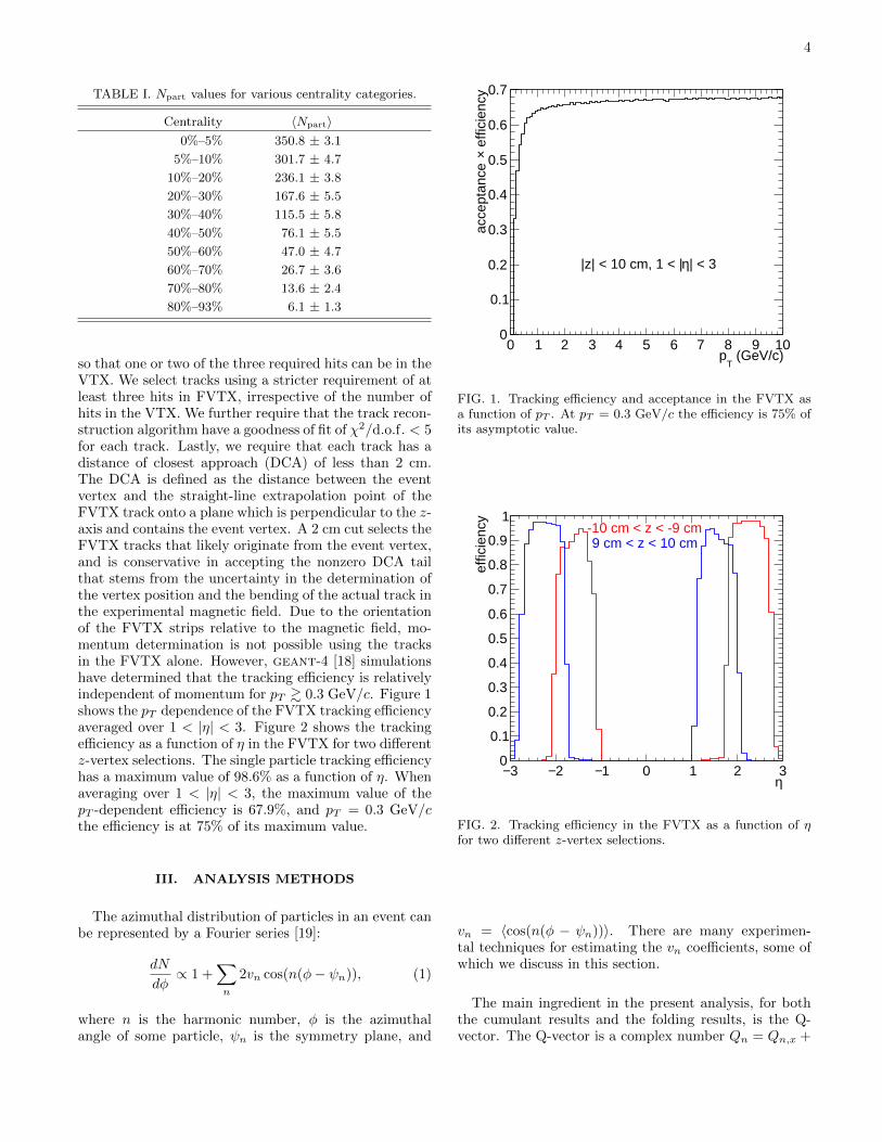
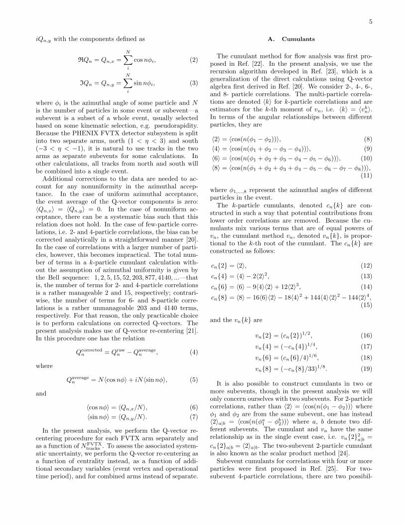
so that one or two of the three required hits can be in theVTX. We select tracks using a stricter requirement of atleast three hits in FVTX, irrespective of the number ofhits in the VTX. We further require that the track recon-struction algorithm have a goodness of fit of χ2/d.o.f. < 5for each track. Lastly, we require that each track has adistance of closest approach (DCA) of less than 2 cm.The DCA is defined as the distance between the eventvertex and the straight-line extrapolation point of theFVTX track onto a plane which is perpendicular to the z-axis and contains the event vertex. A 2 cm cut selects theFVTX tracks that likely originate from the event vertex,and is conservative in accepting the nonzero DCA tailthat stems from the uncertainty in the determination ofthe vertex position and the bending of the actual track inthe experimental magnetic field. Due to the orientationof the FVTX strips relative to the magnetic field, mo-mentum determination is not possible using the tracksin the FVTX alone. However, geant-4 [18] simulationshave determined that the tracking efficiency is relativelyindependent of momentum for pT & 0.3 GeV/c. Figure 1shows the pT dependence of the FVTX tracking efficiencyaveraged over 1 < |η| < 3. Figure 2 shows the trackingefficiency as a function of η in the FVTX for two differentz-vertex selections. The single particle tracking efficiencyhas a maximum value of 98.6% as a function of η. Whenaveraging over 1 < |η| < 3, the maximum value of thepT -dependent efficiency is 67.9%, and pT = 0.3 GeV/cthe efficiency is at 75% of its maximum value.
III. ANALYSIS METHODS
The azimuthal distribution of particles in an event canbe represented by a Fourier series [19]:
dN
dφ∝ 1 +
∑n
2vn cos(n(φ− ψn)), (1)
where n is the harmonic number, φ is the azimuthalangle of some particle, ψn is the symmetry plane, and
(GeV/c)T
p0 1 2 3 4 5 6 7 8 9 10
effi
cien
cy×
acce
ptan
ce
0
0.1
0.2
0.3
0.4
0.5
0.6
0.7
| < 3η|z| < 10 cm, 1 < |
FIG. 1. Tracking efficiency and acceptance in the FVTX asa function of pT . At pT = 0.3 GeV/c the efficiency is 75% ofits asymptotic value.
η3− 2− 1− 0 1 2 3
effic
ienc
y
0
0.1
0.2
0.3
0.4
0.5
0.6
0.7
0.8
0.9
1-10 cm < z < -9 cm9 cm < z < 10 cm
FIG. 2. Tracking efficiency in the FVTX as a function of ηfor two different z-vertex selections.
vn = 〈cos(n(φ − ψn))〉. There are many experimen-tal techniques for estimating the vn coefficients, some ofwhich we discuss in this section.
The main ingredient in the present analysis, for boththe cumulant results and the folding results, is the Q-vector. The Q-vector is a complex number Qn = Qn,x +
5
iQn,y with the components defined as
RQn = Qn,x =
N∑i
cosnφi, (2)
IQn = Qn,y =
N∑i
sinnφi, (3)
where φi is the azimuthal angle of some particle and Nis the number of particles in some event or subevent—asubevent is a subset of a whole event, usually selectedbased on some kinematic selection, e.g. pseudorapidity.Because the PHENIX FVTX detector subsystem is splitinto two separate arms, north (1 < η < 3) and south(−3 < η < −1), it is natural to use tracks in the twoarms as separate subevents for some calculations. Inother calculations, all tracks from north and south willbe combined into a single event.
Additional corrections to the data are needed to ac-count for any nonuniformity in the azimuthal accep-tance. In the case of uniform azimuthal acceptance,the event average of the Q-vector components is zero:〈Qn,x〉 = 〈Qn,y〉 = 0. In the case of nonuniform ac-ceptance, there can be a systematic bias such that thisrelation does not hold. In the case of few-particle corre-lations, i.e. 2- and 4-particle correlations, the bias can becorrected analytically in a straightforward manner [20].In the case of correlations with a larger number of parti-cles, however, this becomes impractical. The total num-ber of terms in a k-particle cumulant calculation with-out the assumption of azimuthal uniformity is given bythe Bell sequence: 1, 2, 5, 15, 52, 203, 877, 4140, ...—thatis, the number of terms for 2- and 4-particle correlationsis a rather manageable 2 and 15, respectively; contrari-wise, the number of terms for 6- and 8-particle corre-lations is a rather unmanageable 203 and 4140 terms,respectively. For that reason, the only practicable choiceis to perform calculations on corrected Q-vectors. Thepresent analysis makes use of Q-vector re-centering [21].In this procedure one has the relation
Qcorrectedn = Qraw
n −Qaveragen , (4)
where
Qaveragen = N〈cosnφ〉+ iN〈sinnφ〉, (5)
and
〈cosnφ〉 = 〈Qn,x/N〉, (6)
〈sinnφ〉 = 〈Qn,y/N〉. (7)
In the present analysis, we perform the Q-vector re-centering procedure for each FVTX arm separately andas a function of NFVTX
tracks . To assess the associated system-atic uncertainty, we perform the Q-vector re-centering asa function of centrality instead, as a function of addi-tional secondary variables (event vertex and operationaltime period), and for combined arms instead of separate.
A. Cumulants
The cumulant method for flow analysis was first pro-posed in Ref. [22]. In the present analysis, we use therecursion algorithm developed in Ref. [23], which is ageneralization of the direct calculations using Q-vectoralgebra first derived in Ref. [20]. We consider 2-, 4-, 6-,and 8- particle correlations. The multi-particle correla-tions are denoted 〈k〉 for k-particle correlations and areestimators for the k-th moment of vn, i.e. 〈k〉 = 〈vkn〉.In terms of the angular relationships between differentparticles, they are
〈2〉 = 〈cos(n(φ1 − φ2))〉, (8)
〈4〉 = 〈cos(n(φ1 + φ2 − φ3 − φ4))〉, (9)
〈6〉 = 〈cos(n(φ1 + φ2 + φ3 − φ4 − φ5 − φ6))〉, (10)
〈8〉 = 〈cos(n(φ1 + φ2 + φ3 + φ4 − φ5 − φ6 − φ7 − φ8))〉,(11)
where φ1,...,8 represent the azimuthal angles of differentparticles in the event.
The k-particle cumulants, denoted cn{k} are con-structed in such a way that potential contributions fromlower order correlations are removed. Because the cu-mulants mix various terms that are of equal powers ofvn, the cumulant method vn, denoted vn{k}, is propor-tional to the k-th root of the cumulant. The cn{k} areconstructed as follows:
cn{2} = 〈2〉, (12)
cn{4} = 〈4〉 − 2〈2〉2, (13)
cn{6} = 〈6〉 − 9〈4〉〈2〉+ 12〈2〉3, (14)
cn{8} = 〈8〉 − 16〈6〉〈2〉 − 18〈4〉2 + 144〈4〉〈2〉2 − 144〈2〉4,(15)
and the vn{k} are
vn{2} = (cn{2})1/2, (16)
vn{4} = (−cn{4})1/4, (17)
vn{6} = (cn{6}/4)1/6, (18)
vn{8} = (−cn{8}/33)1/8. (19)
It is also possible to construct cumulants in two ormore subevents, though in the present analysis we willonly concern ourselves with two subevents. For 2-particlecorrelations, rather than 〈2〉 = 〈cos(n(φ1 − φ2))〉 whereφ1 and φ2 are from the same subevent, one has instead〈2〉a|b = 〈cos(n(φa1 − φb2))〉 where a, b denote two dif-ferent subevents. The cumulant and vn have the samerelationship as in the single event case, i.e. vn{2}2a|b =
cn{2}a|b = 〈2〉a|b. The two-subevent 2-particle cumulantis also known as the scalar product method [24].
Subevent cumulants for correlations with four or moreparticles were first proposed in Ref. [25]. For two-subevent 4-particle correlations, there are two possibil-
6
ities:
〈4〉ab|ab = 〈cos(n(φa1 + φb2 − φa3 − φb4))〉, (20)
〈4〉aa|bb = 〈cos(n(φa1 + φa2 − φb3 − φb4))〉, (21)
where the former allows 2-particle correlations withinsingle subevents and the latter excludes them. The latteris therefore less susceptible to nonflow than the former,although both are less susceptible to nonflow than singleevent 4-particle correlations. The cumulants take theform
cn{4}ab|ab = 〈4〉ab|ab − 〈2〉a|a〈2〉b|b − 〈2〉2a|b, (22)
cn{4}aa|bb = 〈4〉aa|bb − 2〈2〉2a|b, (23)
and the vn{4} values have the same relationship to thecumulants as in the single particle case, i.e. vn{4}ab|ab =
(−cn{4}ab|ab)1/4 and vn{4}aa|bb = (−cn{4}aa|bb)1/4.To determine systematic uncertainties associated with
event and track selection for the cumulant analysis, wevary the event and track selection criteria and assess thevariation on the final analysis results. The z-vertex se-lection is modified from ± 10 cm to ± 5 cm. The trackselections are independently modified to have a goodnessof fit requirement χ2/d.o.f. < 3. These changes movethe cumulant results by an almost common multiplica-tive value and thus we quote the systematic uncertaintiesas a global scale factor uncertainty for each result.
B. Folding
Here we describe an alternative approach where oneutilizes the event-by-event Qn distribution to extract theevent-by-event vn distribution via an unfolding proce-dure. For our analysis we attempt a procedure similar tothat used by ATLAS as described in Ref. [10].
In brief, ATLAS successfully carries out the unfold inPb+Pb collisions at 2.76 TeV and finds that the event-by-event probability distribution for elliptic flow p(v2) isreasonably described by a Bessel-Gaussian function
p(vn) =vnδ2vn
e− (v2n+(vRP
n )2)
2δ2vn I0
(vnv
RPn
δ2vn
), (24)
where vRPn and δ2vn are function parameters that are re-
lated but not equal to the mean and variance of the dis-tribution, respectively. Because flow is a vector quantity,it has both a magnitude and a phase. When measuringvn one measures the modulus of the complex number,meaning there is a reduction in the number of dimensionsfrom two to one. If the fluctuations in each dimensionare Gaussian, one then expects the final distribution ofvalues to be Bessel-Gaussian. Recently the CMS exper-iment has carried out a similar flow unfolding and ob-serves small deviations from the Bessel-Gaussian form,favoring the elliptic power distribution [26].
For the unfolding, ATLAS determines the responsematrix in a data driven way. The smearing in the re-sponse matrix is modest as Pb+Pb collisions have a highmultiplicity and the ATLAS detector has large phasespace coverage for tracks −2.5 < η < +2.5. In our case,the multiplicity of Au+Au collisions is lower in compar-ison with the multiplicity in Pb+Pb collisions and thephase space coverage of the FVTX detector is signifi-cantly smaller. Hence, the smearing as encoded in theresponse matrix is significantly larger and the unfoldingis more challenging.
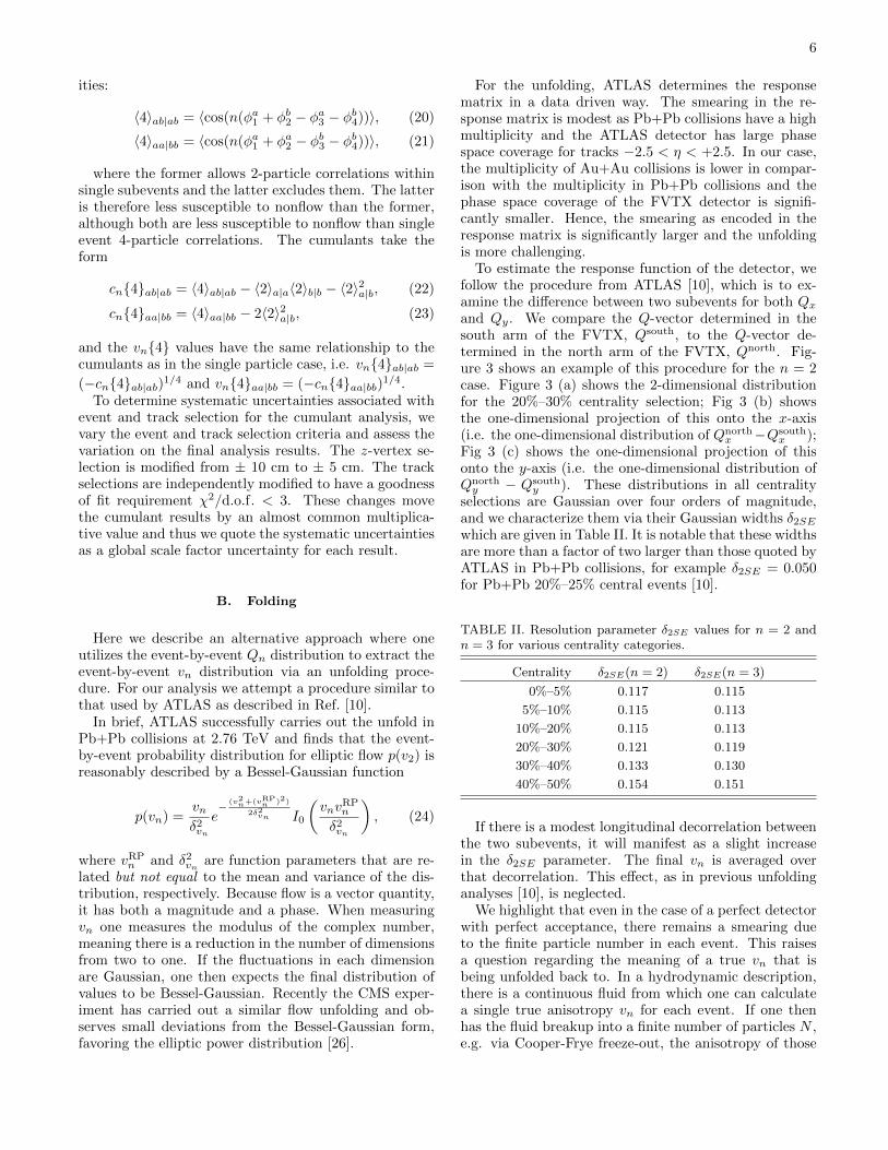
To estimate the response function of the detector, wefollow the procedure from ATLAS [10], which is to ex-amine the difference between two subevents for both Qx
and Qy. We compare the Q-vector determined in thesouth arm of the FVTX, Qsouth, to the Q-vector de-termined in the north arm of the FVTX, Qnorth. Fig-ure 3 shows an example of this procedure for the n = 2case. Figure 3 (a) shows the 2-dimensional distributionfor the 20%–30% centrality selection; Fig 3 (b) showsthe one-dimensional projection of this onto the x-axis(i.e. the one-dimensional distribution of Qnorth
x −Qsouthx );
Fig 3 (c) shows the one-dimensional projection of thisonto the y-axis (i.e. the one-dimensional distribution ofQnorth
y − Qsouthy ). These distributions in all centrality
selections are Gaussian over four orders of magnitude,and we characterize them via their Gaussian widths δ2SE
which are given in Table II. It is notable that these widthsare more than a factor of two larger than those quoted byATLAS in Pb+Pb collisions, for example δ2SE = 0.050for Pb+Pb 20%–25% central events [10].
TABLE II. Resolution parameter δ2SE values for n = 2 andn = 3 for various centrality categories.
Centrality δ2SE(n = 2) δ2SE(n = 3)
0%–5% 0.117 0.115
5%–10% 0.115 0.113
10%–20% 0.115 0.113
20%–30% 0.121 0.119
30%–40% 0.133 0.130
40%–50% 0.154 0.151
If there is a modest longitudinal decorrelation betweenthe two subevents, it will manifest as a slight increasein the δ2SE parameter. The final vn is averaged overthat decorrelation. This effect, as in previous unfoldinganalyses [10], is neglected.
We highlight that even in the case of a perfect detectorwith perfect acceptance, there remains a smearing dueto the finite particle number in each event. This raisesa question regarding the meaning of a true vn that isbeing unfolded back to. In a hydrodynamic description,there is a continuous fluid from which one can calculatea single true anisotropy vn for each event. If one thenhas the fluid breakup into a finite number of particles N ,e.g. via Cooper-Frye freeze-out, the anisotropy of those
7
(South)x(North) - QxQ1− 0.5− 0 0.5 1
(Sou
th)
y(N
orth
) - Q
yQ
1−
0.5−
0
0.5
1
0
100
200
300
400
500
600
700=200 GeVNNsPHENIX Au+Au n=2, 20-30% Central
(South)x(North) - QxQ1− 0.5− 0 0.5 1
1
10
210
310
410 = 0.12092SE,xδ
(South)y
(North) - QyQ1− 0.5− 0 0.5 1
1
10
210
310
410 = 0.12002SE,yδ
(a) (b) (c)
FIG. 3. Example distribution of Qnorth − Qsouth for the n = 2 case corresponding to Au+Au collisions at√sNN = 200 GeV
and centrality 20–30%. (a) The two-dimensional distribution. (b) The projection onto Qx. (c) The projection onto Qy. Shownfor (b) and (c) are the extracted Gaussian widths δ2SE—the χ2/d.o.f. values of the fits are 1.02 and 1.18 for (b) and (c),respectively.
N particles will fluctuate around the true fluid value.However, in a parton scattering description, for exampleampt [27], the time evolution is described in terms ofa finite number of particles N . In this sense there is noseparating of a true vn from that encoded in the N parti-cles themselves. Regardless, one can still mathematicallyapply the unfolding and compare experiment and theoryas manipulated through the same algorithm.
As noted before, the one-dimensional radial projectionof a two-dimensional Gaussian is the so-called Bessel-Gaussian function. In this case it means that the con-ditional probability to measure a value vobsn given a truevalue vn has the following Bessel-Gaussian form:
p(vobsn |vn) ∝ vobsn e−(vobsn )2+v2n
2δ2 I0
(vobsn vnδ2
), (25)
where δ is the smearing parameter characterizing theresponse due to the finite particle number (includingfrom the detector efficiency and acceptance), and I0 isa modified Bessel function of the first kind. The smear-ing parameter δ uses the combination of the two FVTXarms and is related to the result from the difference byδ = δ2SE/2. We highlight that the Bessel-Gaussian inEqn. 25 is different from the Bessel-Gaussian in Eqn. 24,though both arise from a similar dimensional reduction.
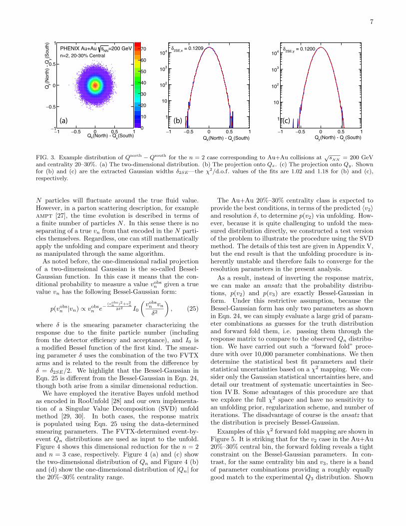
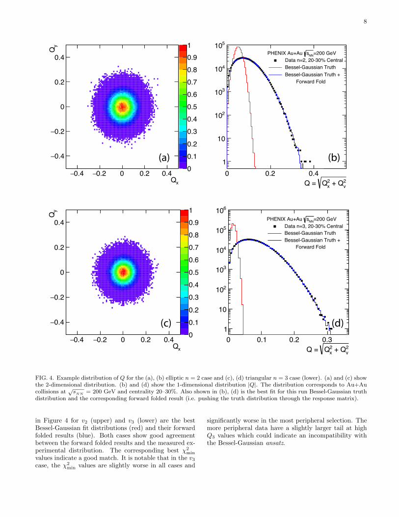
We have employed the iterative Bayes unfold methodas encoded in RooUnfold [28] and our own implementa-tion of a Singular Value Decomposition (SVD) unfoldmethod [29, 30]. In both cases, the response matrixis populated using Eqn. 25 using the data-determinedsmearing parameters. The FVTX-determined event-by-event Qn distributions are used as input to the unfold.Figure 4 shows this dimensional reduction for the n = 2and n = 3 case, respectively. Figure 4 (a) and (c) showthe two-dimensional distribution of Qn and Figure 4 (b)and (d) show the one-dimensional distribution of |Qn| forthe 20%–30% centrality range.
The Au+Au 20%–30% centrality class is expected toprovide the best conditions, in terms of the predicted 〈v2〉and resolution δ, to determine p(v2) via unfolding. How-ever, because it is quite challenging to unfold the mea-sured distribution directly, we constructed a test versionof the problem to illustrate the procedure using the SVDmethod. The details of this test are given in Appendix V,but the end result is that the unfolding procedure is in-herently unstable and therefore fails to converge for theresolution parameters in the present analysis.
As a result, instead of inverting the response matrix,we can make an ansatz that the probability distribu-tions, p(v2) and p(v3) are exactly Bessel-Gaussian inform. Under this restrictive assumption, because theBessel-Gaussian form has only two parameters as shownin Eqn. 24, we can simply evaluate a large grid of param-eter combinations as guesses for the truth distributionand forward fold them, i.e. passing them through theresponse matrix to compare to the observed Qn distribu-tion. We have carried out such a “forward fold” proce-dure with over 10,000 parameter combinations. We thendetermine the statistical best fit parameters and theirstatistical uncertainties based on a χ2 mapping. We con-sider only the Gaussian statistical uncertainties here, anddetail our treatment of systematic uncertainties in Sec-tion IV B. Some advantages of this procedure are thatwe explore the full χ2 space and have no sensitivity toan unfolding prior, regularization scheme, and number ofiterations. The disadvantage of course is the ansatz thatthe distribution is precisely Bessel-Gaussian.
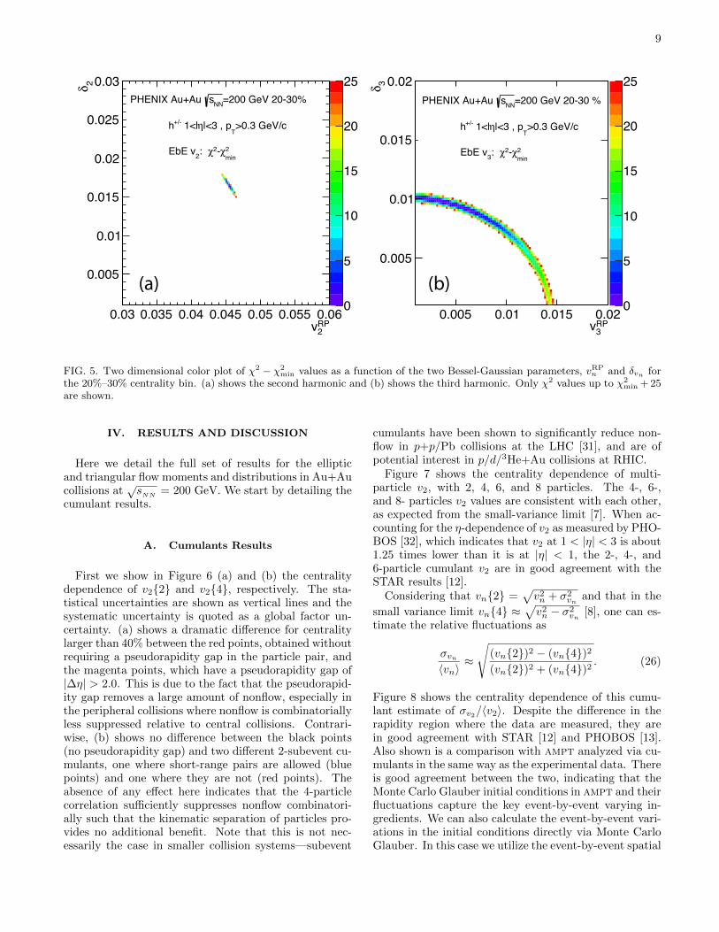
Examples of this χ2 forward fold mapping are shown inFigure 5. It is striking that for the v2 case in the Au+Au20%–30% central bin, the forward folding reveals a tightconstraint on the Bessel-Gaussian parameters. In con-trast, for the same centrality bin and v3, there is a bandof parameter combinations providing a roughly equallygood match to the experimental Q3 distribution. Shown
8
xQ0.4− 0.2− 0 0.2 0.4
yQ
0.4−
0.2−
0
0.2
0.4
00.10.20.30.40.50.60.70.80.91
2y + Q2
xQQ = 0 0.2 0.4
1
10
210
310
410
510=200 GeVNNsPHENIX Au+Au
Data n=2, 20-30% CentralBessel-Gaussian TruthBessel-Gaussian Truth + Forward Fold
(a) (b)
xQ0.4− 0.2− 0 0.2 0.4
yQ
0.4−
0.2−
0
0.2
0.4
00.10.20.30.40.50.60.70.80.91
2y + Q2
xQQ = 0 0.1 0.2 0.3
1
10
210
310
410
510
610=200 GeVNNsPHENIX Au+Au
Data n=3, 20-30% CentralBessel-Gaussian TruthBessel-Gaussian Truth + Forward Fold
(c) (d)
FIG. 4. Example distribution of Q for the (a), (b) elliptic n = 2 case and (c), (d) triangular n = 3 case (lower). (a) and (c) showthe 2-dimensional distribution. (b) and (d) show the 1-dimensional distribution |Q|. The distribution corresponds to Au+Aucollisions at
√sNN = 200 GeV and centrality 20–30%. Also shown in (b), (d) is the best fit for this run Bessel-Gaussian truth
distribution and the corresponding forward folded result (i.e. pushing the truth distribution through the response matrix).
in Figure 4 for v2 (upper) and v3 (lower) are the bestBessel-Gaussian fit distributions (red) and their forwardfolded results (blue). Both cases show good agreementbetween the forward folded results and the measured ex-perimental distribution. The corresponding best χ2
min
values indicate a good match. It is notable that in the v3case, the χ2
min values are slightly worse in all cases and
significantly worse in the most peripheral selection. Themore peripheral data have a slightly larger tail at highQ3 values which could indicate an incompatibility withthe Bessel-Gaussian ansatz.
9
RP2v
0.03 0.035 0.04 0.045 0.05 0.055 0.06
2δ
0.005
0.01
0.015
0.02
0.025
0.03
0
5
10
15
20
25=200 GeV 20-30%NNsPHENIX Au+Au
>0.3 GeV/cT
|<3 , pη 1<|+/-h
min2χ-2χ:2EbE v
RP3v
0.005 0.01 0.015 0.02
3δ
0.005
0.01
0.015
0.02
0
5
10
15
20
25=200 GeV 20-30 %NNsPHENIX Au+Au
>0.3 GeV/cT
|<3 , pη 1<|+/-h
min2χ-2χ:3EbE v
(a) (b)
FIG. 5. Two dimensional color plot of χ2 − χ2min values as a function of the two Bessel-Gaussian parameters, vRP
n and δvn forthe 20%–30% centrality bin. (a) shows the second harmonic and (b) shows the third harmonic. Only χ2 values up to χ2
min + 25are shown.
IV. RESULTS AND DISCUSSION
Here we detail the full set of results for the ellipticand triangular flow moments and distributions in Au+Aucollisions at
√sNN
= 200 GeV. We start by detailing thecumulant results.
A. Cumulants Results
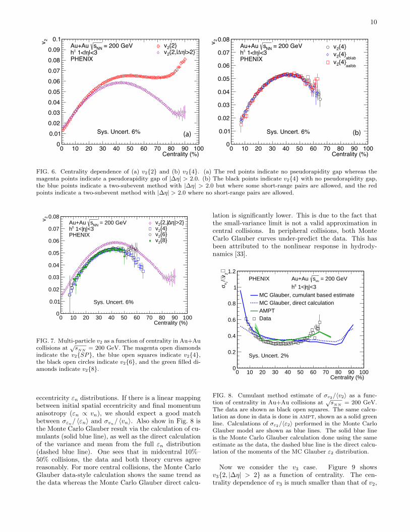
First we show in Figure 6 (a) and (b) the centralitydependence of v2{2} and v2{4}, respectively. The sta-tistical uncertainties are shown as vertical lines and thesystematic uncertainty is quoted as a global factor un-certainty. (a) shows a dramatic difference for centralitylarger than 40% between the red points, obtained withoutrequiring a pseudorapidity gap in the particle pair, andthe magenta points, which have a pseudorapidity gap of|∆η| > 2.0. This is due to the fact that the pseudorapid-ity gap removes a large amount of nonflow, especially inthe peripheral collisions where nonflow is combinatoriallyless suppressed relative to central collisions. Contrari-wise, (b) shows no difference between the black points(no pseudorapidity gap) and two different 2-subevent cu-mulants, one where short-range pairs are allowed (bluepoints) and one where they are not (red points). Theabsence of any effect here indicates that the 4-particlecorrelation sufficiently suppresses nonflow combinatori-ally such that the kinematic separation of particles pro-vides no additional benefit. Note that this is not nec-essarily the case in smaller collision systems—subevent
cumulants have been shown to significantly reduce non-flow in p+p/Pb collisions at the LHC [31], and are ofpotential interest in p/d/3He+Au collisions at RHIC.
Figure 7 shows the centrality dependence of multi-particle v2, with 2, 4, 6, and 8 particles. The 4-, 6-,and 8- particles v2 values are consistent with each other,as expected from the small-variance limit [7]. When ac-counting for the η-dependence of v2 as measured by PHO-BOS [32], which indicates that v2 at 1 < |η| < 3 is about1.25 times lower than it is at |η| < 1, the 2-, 4-, and6-particle cumulant v2 are in good agreement with theSTAR results [12].
Considering that vn{2} =√v2n + σ2
vn and that in the
small variance limit vn{4} ≈√v2n − σ2
vn [8], one can es-timate the relative fluctuations as
σvn〈vn〉
≈
√(vn{2})2 − (vn{4})2(vn{2})2 + (vn{4})2
. (26)
Figure 8 shows the centrality dependence of this cumu-lant estimate of σv2/〈v2〉. Despite the difference in therapidity region where the data are measured, they arein good agreement with STAR [12] and PHOBOS [13].Also shown is a comparison with ampt analyzed via cu-mulants in the same way as the experimental data. Thereis good agreement between the two, indicating that theMonte Carlo Glauber initial conditions in ampt and theirfluctuations capture the key event-by-event varying in-gredients. We can also calculate the event-by-event vari-ations in the initial conditions directly via Monte CarloGlauber. In this case we utilize the event-by-event spatial
10
Centrality (%)0 10 20 30 40 50 60 70 80 90 100
2v
00.010.020.030.040.050.060.070.080.09
0.1
PHENIX|<3η 1<|±h
= 200 GeVNNsAu+Au
Sys. Uncert. 6%
{2}2v|>2}η∆{2,|2v
(a)
Centrality (%)0 10 20 30 40 50 60 70 80 90 100
2v
0
0.01
0.02
0.03
0.04
0.05
0.06
0.07
0.08
PHENIX|<3η 1<|±h
= 200 GeVNNsAu+Au
Sys. Uncert. 6%
{4}2vab|ab
{4}2v
aa|bb{4}2v
(b)
FIG. 6. Centrality dependence of (a) v2{2} and (b) v2{4}. (a) The red points indicate no pseudorapidity gap whereas themagenta points indicate a pseudorapidity gap of |∆η| > 2.0. (b) The black points indicate v2{4} with no pseudorapidity gap,the blue points indicate a two-subevent method with |∆η| > 2.0 but where some short-range pairs are allowed, and the redpoints indicate a two-subevent method with |∆η| > 2.0 where no short-range pairs are allowed.
Centrality (%)0 10 20 30 40 50 60 70 80 90 100
2v
0
0.01
0.02
0.03
0.04
0.05
0.06
0.07
0.08
PHENIX|<3η 1<|±h
= 200 GeVNNsAu+Au
Sys. Uncert. 6%
|>2}η∆{2,|2v{4}2v{6}2v{8}2v
FIG. 7. Multi-particle v2 as a function of centrality in Au+Aucollisions at
√sNN = 200 GeV. The magenta open diamonds
indicate the v2{SP}, the blue open squares indicate v2{4},the black open circles indicate v2{6}, and the green filled di-amonds indicate v2{8}.
eccentricity εn distributions. If there is a linear mappingbetween initial spatial eccentricity and final momentumanisotropy (εn ∝ vn), we should expect a good matchbetween σεn/ 〈εn〉 and σvn/ 〈vn〉. Also show in Fig. 8 isthe Monte Carlo Glauber result via the calculation of cu-mulants (solid blue line), as well as the direct calculationof the variance and mean from the full εn distribution(dashed blue line). One sees that in midcentral 10%–50% collisions, the data and both theory curves agreereasonably. For more central collisions, the Monte CarloGlauber data-style calculation shows the same trend asthe data whereas the Monte Carlo Glauber direct calcu-
lation is significantly lower. This is due to the fact thatthe small-variance limit is not a valid approximation incentral collisions. In peripheral collisions, both MonteCarlo Glauber curves under-predict the data. This hasbeen attributed to the nonlinear response in hydrody-namics [33].
Centrality (%)0 10 20 30 40 50 60 70 80 90 100
⟩ 2v⟨/2vσ
0
0.2
0.4
0.6
0.8
1
1.2PHENIX = 200 GeV
NNsAu+Au
|<3η 1<|±h
Sys. Uncert. 2%
MC Glauber, cumulant based estimateMC Glauber, direct calculationAMPTData
FIG. 8. Cumulant method estimate of σv2/〈v2〉 as a func-tion of centrality in Au+Au collisions at
√sNN = 200 GeV.
The data are shown as black open squares. The same calcu-lation as done in data is done in ampt, shown as a solid greenline. Calculations of σε2/〈ε2〉 performed in the Monte CarloGlauber model are shown as blue lines. The solid blue lineis the Monte Carlo Glauber calculation done using the sameestimate as the data, the dashed blue line is the direct calcu-lation of the moments of the MC Glauber ε2 distribution.
Now we consider the v3 case. Figure 9 showsv3{2, |∆η| > 2} as a function of centrality. The cen-trality dependence of v3 is much smaller than that of v2,
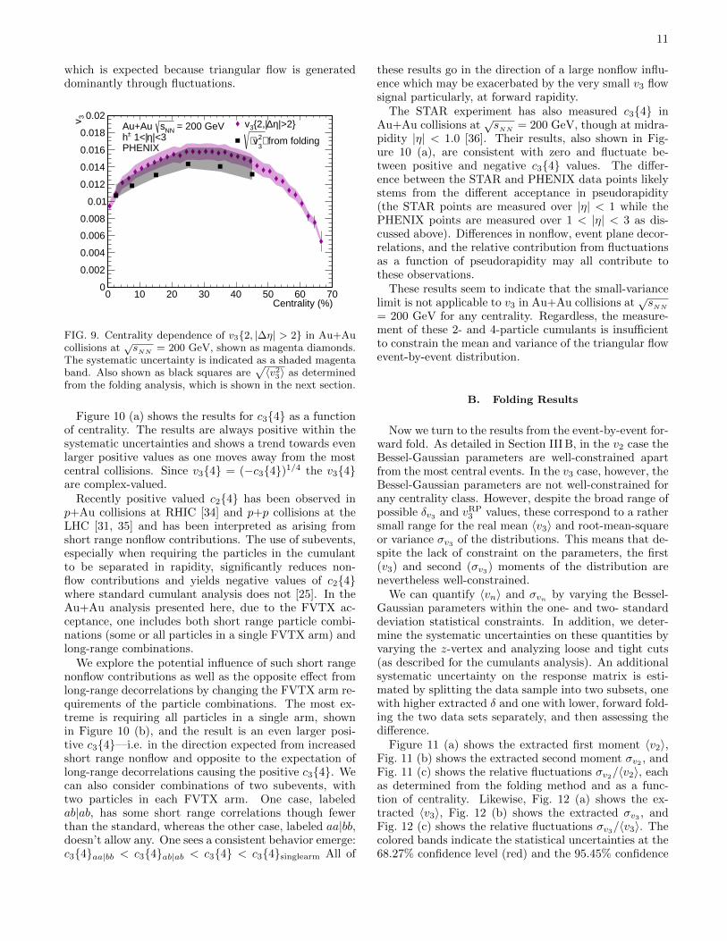
11
which is expected because triangular flow is generateddominantly through fluctuations.
Centrality (%)0 10 20 30 40 50 60 70
3v
0
0.002
0.004
0.006
0.008
0.01
0.012
0.014
0.016
0.018
0.02
PHENIX|<3η 1<|±h
= 200 GeVNNsAu+Au |>2}η∆{2,|3v
from folding⟩23
v⟨
FIG. 9. Centrality dependence of v3{2, |∆η| > 2} in Au+Aucollisions at
√sNN = 200 GeV, shown as magenta diamonds.
The systematic uncertainty is indicated as a shaded magentaband. Also shown as black squares are
√〈v23〉 as determined
from the folding analysis, which is shown in the next section.
Figure 10 (a) shows the results for c3{4} as a functionof centrality. The results are always positive within thesystematic uncertainties and shows a trend towards evenlarger positive values as one moves away from the mostcentral collisions. Since v3{4} = (−c3{4})1/4 the v3{4}are complex-valued.
Recently positive valued c2{4} has been observed inp+Au collisions at RHIC [34] and p+p collisions at theLHC [31, 35] and has been interpreted as arising fromshort range nonflow contributions. The use of subevents,especially when requiring the particles in the cumulantto be separated in rapidity, significantly reduces non-flow contributions and yields negative values of c2{4}where standard cumulant analysis does not [25]. In theAu+Au analysis presented here, due to the FVTX ac-ceptance, one includes both short range particle combi-nations (some or all particles in a single FVTX arm) andlong-range combinations.
We explore the potential influence of such short rangenonflow contributions as well as the opposite effect fromlong-range decorrelations by changing the FVTX arm re-quirements of the particle combinations. The most ex-treme is requiring all particles in a single arm, shownin Figure 10 (b), and the result is an even larger posi-tive c3{4}—i.e. in the direction expected from increasedshort range nonflow and opposite to the expectation oflong-range decorrelations causing the positive c3{4}. Wecan also consider combinations of two subevents, withtwo particles in each FVTX arm. One case, labeledab|ab, has some short range correlations though fewerthan the standard, whereas the other case, labeled aa|bb,doesn’t allow any. One sees a consistent behavior emerge:c3{4}aa|bb < c3{4}ab|ab < c3{4} < c3{4}singlearm All of
these results go in the direction of a large nonflow influ-ence which may be exacerbated by the very small v3 flowsignal particularly, at forward rapidity.
The STAR experiment has also measured c3{4} inAu+Au collisions at
√sNN
= 200 GeV, though at midra-pidity |η| < 1.0 [36]. Their results, also shown in Fig-ure 10 (a), are consistent with zero and fluctuate be-tween positive and negative c3{4} values. The differ-ence between the STAR and PHENIX data points likelystems from the different acceptance in pseudorapidity(the STAR points are measured over |η| < 1 while thePHENIX points are measured over 1 < |η| < 3 as dis-cussed above). Differences in nonflow, event plane decor-relations, and the relative contribution from fluctuationsas a function of pseudorapidity may all contribute tothese observations.
These results seem to indicate that the small-variancelimit is not applicable to v3 in Au+Au collisions at
√sNN
= 200 GeV for any centrality. Regardless, the measure-ment of these 2- and 4-particle cumulants is insufficientto constrain the mean and variance of the triangular flowevent-by-event distribution.
B. Folding Results
Now we turn to the results from the event-by-event for-ward fold. As detailed in Section III B, in the v2 case theBessel-Gaussian parameters are well-constrained apartfrom the most central events. In the v3 case, however, theBessel-Gaussian parameters are not well-constrained forany centrality class. However, despite the broad range ofpossible δv3 and vRP
3 values, these correspond to a rathersmall range for the real mean 〈v3〉 and root-mean-squareor variance σv3 of the distributions. This means that de-spite the lack of constraint on the parameters, the first(v3) and second (σv3) moments of the distribution arenevertheless well-constrained.
We can quantify 〈vn〉 and σvn by varying the Bessel-Gaussian parameters within the one- and two- standarddeviation statistical constraints. In addition, we deter-mine the systematic uncertainties on these quantities byvarying the z-vertex and analyzing loose and tight cuts(as described for the cumulants analysis). An additionalsystematic uncertainty on the response matrix is esti-mated by splitting the data sample into two subsets, onewith higher extracted δ and one with lower, forward fold-ing the two data sets separately, and then assessing thedifference.
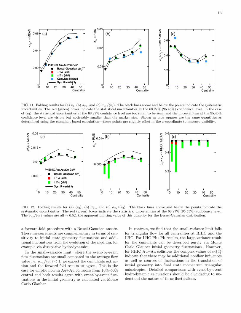
Figure 11 (a) shows the extracted first moment 〈v2〉,Fig. 11 (b) shows the extracted second moment σv2 , andFig. 11 (c) shows the relative fluctuations σv2/〈v2〉, eachas determined from the folding method and as a func-tion of centrality. Likewise, Fig. 12 (a) shows the ex-tracted 〈v3〉, Fig. 12 (b) shows the extracted σv3 , andFig. 12 (c) shows the relative fluctuations σv3/〈v3〉. Thecolored bands indicate the statistical uncertainties at the68.27% confidence level (red) and the 95.45% confidence

12
0 10 20 30 40 50 60Centrality (%)
0.1−
0.05−
0
0.05
0.1
0.156−10×
{4}
3c
PHENIX|<3η 1<|±h
= 200 GeVNNsAu+Au
{4}3c
ab|ab{4}3c
aa|bb{4}3c
|<1ηSTAR |(a)
0 10 20 30 40 50 60Centrality (%)
0.1−
0
0.1
0.2
0.3
0.4
0.56−10×
{4}
3c
PHENIX|<3η 1<|±h
= 200 GeVNNsAu+Au Combined arms
Single arm
(b)
FIG. 10. Centrality dependence of c3{4} for Au+Au collisions at√sNN = 200 GeV. (a) Calculations using both arms: c3{4}
(black circles), c3{4}ab|ab (blue diamonds), c3{4}aa|bb (red squares), and comparison to STAR [36] (black stars). (b) Comparisonof c3{4} determined using both arms (open symbols) and a single arm (closed symbols). Note that the open black circles arethe same in (a) and (b).
level (green) from the χ2 analysis. The thin black lines in-dicate the systematic uncertainties. Also shown in 11 asblue squares are results from the cumulant based calcula-tion as discussed in the previous section. The 〈v2〉 valuesare in excellent agreement for all centralities, and theσv2 and σv2/〈v2〉 are in reasonable agreement for 10%–50% centrality, where the small-variance limit holds. Fig-ure 9 shows a comparison between the cumulant resultv3{2, |∆η| > 2|} and the folding analysis result
√〈v23〉
(calculated from the results in Fig. 12). These resultsare consistent within the systematic uncertainties.
We highlight that the σv2/〈v2〉 values agree well withthose determined from the cumulant method as shownin Figure 8, except in the most central and peripheralAu+Au events. The most central 0%–5% events are ex-actly where the Monte Carlo Glauber results in Figure 8indicate a breakdown in the small-variance approxima-tion. This is a good validation of the forward folding pro-cedure and another confirmation that the event-by-eventelliptic flow fluctuations in Au+Au collisions at
√sNN
=200 GeV are dominated by initial geometry fluctuations.
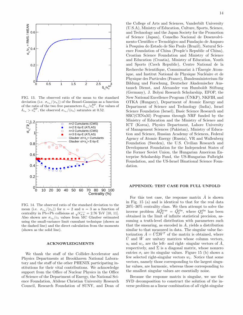
Intriguingly, whereas the values of σv2/〈v2〉 vary signif-icantly as a function of centrality, the values of σv3/〈v3〉are almost precisely 0.52 independent of centrality. Tounderstand this better, we need to consider a rather pe-culiar feature of the Bessel-Gaussian Function. Figure 13shows the σvn/〈vn〉 of the Bessel-Gaussian as a functionof the ratio δ/vRP
n . For values of δ > vRPn , the observed
σvn/〈vn〉 saturates at a value of about 0.52. Thus, anyBessel-Gaussian in the large variance limit will have aσvn/〈vn〉 of the same value.
This observation can, in fact, help shed light on theobserved discrepancy between the CMS [11] and AT-LAS [10] data on σv3/〈v3〉. Figure 14 shows σv2/〈v2〉and σv3/〈v3〉 as a function of centrality in Pb+Pb colli-sions at
√sNN
= 2.76 TeV from CMS and ATLAS. The
CMS results are obtained using the cumulant method as-suming the small-variance limit. In contrast the ATLASresults are obtained via an event-by-event unfolding andcalculating the exact mean and variance of the distribu-tion.
The σv2/〈v2〉 values are in very good agreement, whichappears to validate the small variance approximation (aswas also validated in the Au+Au at
√sNN
= 200 GeVcase in this analysis). In contrast, there is a large differ-ence in the σv3/〈v3〉 between the different methods. TheATLAS σv3
/〈v3〉 values are all very close to 0.52, ex-actly as observed above in the present Au+Au data andas found to be a limiting case for the Bessel-Gaussianfunction. To better understand the σv3
/〈v3〉, we alsoshow σε3/〈ε3〉 as determined from MC Glauber calcula-tions. The dashed red-line uses the small-variance limitestimate with cumulants, as is done for the CMS data,and the agreement is quite reasonable. The solid redline is calculated from the moments of the ε3 distribu-tion directly, and shows good agreement with the AT-LAS data. This represents a quantitative confirmationof the event-by-event fluctuations and the breakdown inthe small variance approximation. The v3{4} at forwardrapidity at RHIC is found to be complex-valued, whichmay be the result of a very small flow v3 and significantnonflow contributions.
V. SUMMARY AND CONCLUSIONS
In summary, we have presented measurements of ellip-tic and triangular flow in Au+Au collisions at 200 GeVfor charged hadrons at forward rapidity 1 < |η| < 3.In particular, we compare flow cumulants (v2{2}, v2{4},v2{6}, v2{8} and v3{2}, v3{4}) and the mean and vari-ance of the v2 and v3 event-by-event distributions using
13
Centrality0 10 20 30 40 50
> =
MEA
N2
<v
0
0.02
0.04
0.06
PHENIX Au+Au 200 GeV)
2Bessel-Gaussian p(v
(stat)σ 1 ± (stat)σ 2 ±
Cumulant MethodSys. Uncertainty
PHENIX Au+Au 200 GeV)
2Bessel-Gaussian p(v
(stat)σ 1 ± (stat)σ 2 ±
Cumulant MethodSys. Uncertainty
Centrality0 10 20 30 40 50
= R
MS
2vσ
0
0.01
0.02
0.03
Centrality0 10 20 30 40 50
> =
RM
S / M
EAN
2/<
v2vσ
0
0.2
0.4
0.6
(a) (b) (c)
FIG. 11. Folding results for (a) v2, (b) σv2 , and (c) σv2/〈v2〉. The black lines above and below the points indicate the systematicuncertainties. The red (green) boxes indicate the statistical uncertainties at the 68.27% (95.45%) confidence level. In the caseof 〈v2〉, the statistical uncertainties at the 68.27% confidence level are too small to be seen, and the uncertainties at the 95.45%confidence level are visible but noticeably smaller than the marker size. Shown as blue squares are the same quantities asdetermined using the cumulant based calculation—these points are slightly offset in the x-coordinate to improve visibility.
Centrality0 10 20 30 40 50
> =
MEA
N3
<v
0
0.005
0.01
0.015
0.02
PHENIX Au+Au 200 GeV)
3Bessel-Gaussian p(v
(stat)σ 1 ± (stat)σ 2 ±
Sys. Uncertainty
PHENIX Au+Au 200 GeV)
3Bessel-Gaussian p(v
(stat)σ 1 ± (stat)σ 2 ±
Sys. Uncertainty
Centrality0 10 20 30 40 50
= R
MS
3vσ
0
0.005
0.01
Centrality0 10 20 30 40 50
> =
RM
S / M
EAN
3/<
v3vσ
0
0.2
0.4
0.6(a) (b) (c)
FIG. 12. Folding results for (a) 〈v3〉, (b) σv3 , and (c) σv3/〈v3〉. The black lines above and below the points indicate thesystematic uncertainties. The red (green) boxes indicate the statistical uncertainties at the 68.27% (95.45%) confidence level.The σv3/〈v3〉 values are all ≈ 0.52, the apparent limiting value of this quantity for the Bessel-Gaussian distribution.
a forward-fold procedure with a Bessel-Gaussian ansatz.These measurements are complementary in terms of sen-sitivity to initial state geometry fluctuations and addi-tional fluctuations from the evolution of the medium, forexample via dissipative hydrodynamics.
In the small-variance limit, where the event-by-eventflow fluctuations are small compared to the average flowvalue i.e. σvn/〈vn〉 < 1, we expect the cumulants extrac-tion and the forward-fold results to agree. This is thecase for elliptic flow in Au+Au collisions from 10%–50%central and both results agree with event-by-event fluc-tuations in the initial geometry as calculated via MonteCarlo Glauber.
In contrast, we find that the small-variance limit failsfor triangular flow for all centralities at RHIC and theLHC. For LHC Pb+Pb results, the large-variance resultfor the cumulants can be described purely via MonteCarlo Glauber initial geometry fluctuations. However,for RHIC Au+Au collisions the complex values of v3{4}indicate that there may be additional nonflow influencesas well as sources of fluctuations in the translation ofinitial geometry into final state momentum triangularanisotropies. Detailed comparisons with event-by-eventhydrodynamic calculations should be elucidating to un-derstand the nature of these fluctuations.
14
RPn/v
nvδ0 0.5 1 1.5 2 2.5 3
= R
MS
/ M
EA
Nn
/v nvσ
0
0.2
0.4
0.6
FIG. 13. The observed ratio of the mean to the standarddeviation (i.e. σvn/〈vn〉) of the Bessel-Gaussian as a functionof the ratio of the two free parameters δvn/v
RPn . For values of
δvn > vRPn , the observed σvn/〈vn〉 saturates at 0.52.
Centrality (%)0 10 20 30 40 50 60 70 80 90 100
⟩ nv⟨/ nvσ
0
0.2
0.4
0.6
0.8
1
1.2 n=2 Cumulants (CMS)n=2 E-by-E (ATLAS)n=3 Cumulants (CMS) n=3 E-by-E (ATLAS)
> Cumulants3ε/<σGlauber > E-by-E3ε/<σGlauber
FIG. 14. The observed ratio of the standard deviation to themean (i.e. σvn/〈vn〉) for n = 2 and n = 3 as a function ofcentrality in Pb+Pb collisions at
√sNN = 2.76 TeV [10, 11].
Also shown are σε3/ε3 values from MC Glauber estimatedusing the small-variance limit cumulant technique (shown asthe dashed line) and the direct calculation from the moments(shown as the solid line).
ACKNOWLEDGMENTS
We thank the staff of the Collider-Accelerator andPhysics Departments at Brookhaven National Labora-tory and the staff of the other PHENIX participating in-stitutions for their vital contributions. We acknowledgesupport from the Office of Nuclear Physics in the Officeof Science of the Department of Energy, the National Sci-ence Foundation, Abilene Christian University ResearchCouncil, Research Foundation of SUNY, and Dean of
the College of Arts and Sciences, Vanderbilt University(U.S.A), Ministry of Education, Culture, Sports, Science,and Technology and the Japan Society for the Promotionof Science (Japan), Conselho Nacional de Desenvolvi-mento Cientıfico e Tecnologico and Fundacao de Amparoa Pesquisa do Estado de Sao Paulo (Brazil), Natural Sci-ence Foundation of China (People’s Republic of China),Croatian Science Foundation and Ministry of Scienceand Education (Croatia), Ministry of Education, Youthand Sports (Czech Republic), Centre National de la
Recherche Scientifique, Commissariat a l’Energie Atom-ique, and Institut National de Physique Nucleaire et dePhysique des Particules (France), Bundesministerium furBildung und Forschung, Deutscher Akademischer Aus-tausch Dienst, and Alexander von Humboldt Stiftung(Germany), J. Bolyai Research Scholarship, EFOP, the
New National Excellence Program (UNKP), NKFIH, andOTKA (Hungary), Department of Atomic Energy andDepartment of Science and Technology (India), IsraelScience Foundation (Israel), Basic Science Research andSRC(CENuM) Programs through NRF funded by theMinistry of Education and the Ministry of Science andICT (Korea), Physics Department, Lahore Universityof Management Sciences (Pakistan), Ministry of Educa-tion and Science, Russian Academy of Sciences, FederalAgency of Atomic Energy (Russia), VR and WallenbergFoundation (Sweden), the U.S. Civilian Research andDevelopment Foundation for the Independent States ofthe Former Soviet Union, the Hungarian American En-terprise Scholarship Fund, the US-Hungarian FulbrightFoundation, and the US-Israel Binational Science Foun-dation.
APPENDIX: TEST CASE FOR FULL UNFOLD
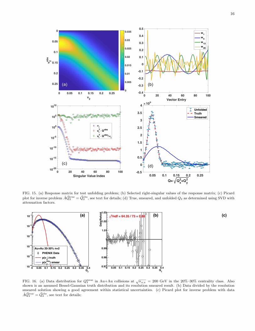
For this test case, the response matrix A is shownin Fig. 15 (a) and is identical to that for the real data20%–30% centrality class. We then attempt to solve the
inverse problem A ~Qtrue2 = ~Qobs
2 , where Qobs2 has been
obtained in the limit of infinite statistical precision, as-suming a truth-level distribution with parameters suchthat the smearing, as encoded in A, yields a distributionsimilar to that measured in data. The singular value fac-torization A = U ΣWT of the matrix is obtained, whereU and W are unitary matrices whose column vectors,ui and wi, are the left- and right- singular vectors of A,respectively, and Σ is a diagonal matrix, whose nonzeroentries σi are its singular values. Figure 15 (b) shows afew selected right-singular vectors wi. Notice that somevectors, namely those corresponding to the largest singu-lar values, are harmonic, whereas those corresponding tothe smallest singular values are essentially noise.
Because the response matrix is singular, we use theSVD decomposition to construct the solution of the in-verse problem as a linear combination of all right-singular
15
vectors, as follows:
~Q2 =
Dim(A)∑i=1
ϕi
(~uTi · ~Qobs
2
σi
)~wi. (27)
The damping factors ϕi = σ2i /(σ
2i +λ2), for some λ ∈ R,
are introduced to attenuate the contribution of the noisysingular vectors to the sum. It is important to point outthat in most implementations of SVD used in high-energyphysics, including RooUnfold, the above sum is simplytruncated to include only a subset of the harmonic sin-gular vectors, potentially leading to loss of information.
To determine which singular vectors contribute to thesolution in a meaningful manner, it is useful to examinethe Picard plot [37] for the problem at hand, shown in
Fig. 15 (c), which displays the singular values σi of A, as
well as the projection of ~Qobs2 onto the singular vectors
~uTi · ~Qobs2 , and the solution coefficients ~uTi · ~Qobs
2 /σi. No-tice that the singular values and the Fourier coefficientsdrop sharply many orders of magnitude before levelingoff, yet in such a way that their ratio is roughly con-stant. The implication is then that all singular vectorsappear to contribute equally to the solution, which isclearly problematic given the noisy nature of most ofthem. In general, it is desirable for Fourier coefficientsto drop off faster than the singular values (to fulfill theso-called discrete Picard condition), such that the Picardplot will reveal the appropriate set of terms to include inthe solution, as identified by a sharp drop in the solutioncoefficients.
Given that our problem does not satisfy the Pi-card condition, we introduce the attenuation factors ϕi
in Eqn. 27. The resulting unfolded Q2 is shown in
Fig. 15 (d), along with the true Qtrue2 , and smeared Qobs
2 .We observe that the unfolding works well, yielding a gooddescription of the true distribution shape, with uncer-tainties associated with varying the regularization pa-rameter λ.
However, in this case the unfolding procedure consti-tutes an ill-posed inverse problem, such that small per-turbations in the input vector—that is, Qobs
2 —translateto very large errors in the solution, compounded by thefact that the Picard condition is violated. In particular,we have verified with our test problem that the statisti-cal fluctuations in Qobs
2 when sampling a finite numberof events, comparable to those recorded in data, indeedlimit the number of available harmonic singular vectors,thus causing the solution to be dominated by noise.
We now examine the application of the above unfoldingmethod to data. Fig. 16 (a) shows an ansatz for Qtrue
2
assuming a Bessel-Gaussian form, and the correspondingrefolded smeared distribution. It compares very well tothe data, as shown in the ratio plot in Fig. 16 (b). Inprinciple, given the good quality of the fit, one wouldexpect the unfolding procedure to work with the data asinput. However, the statistical fluctuations apparent inthe ratio plot perturb the solution in such a way that thenoisy nonharmonic singular vectors are enhanced evenmore than in the test problem, as shown in Fig. 16 (c).As a result, the number of available harmonic singularvectors is reduced, and the problem has no satisfactorysolution, even when regularization is applied. Thus, tobe explicit, the unfolding procedure fails. We note thatif we apply our test example with a significantly betterresolution, i.e. as in the ATLAS Pb+Pb case, the methoddoes converge as expected.
[1] K. Adcox et al. (PHENIX Collaboration), “Formation ofdense partonic matter in relativistic nucleus-nucleus colli-sions at RHIC: Experimental evaluation by the PHENIXcollaboration,” Nucl. Phys. A 757, 184 (2005).
[2] J. Adams et al. (STAR Collaboration), “Experimentaland theoretical challenges in the search for the quarkgluon plasma: The STAR Collaboration’s critical assess-ment of the evidence from RHIC collisions,” Nucl. Phys.A 757, 102 (2005).
[3] B. B. Back et al. (PHOBOS Collaboration), “The PHO-BOS perspective on discoveries at RHIC,” Nucl. Phys. A757, 28 (2005).
[4] I. Arsene et al. (BRAHMS Collaboration), “Quark gluonplasma and color glass condensate at RHIC? The Per-spective from the BRAHMS experiment,” Nucl. Phys. A757, 1 (2005).
[5] P. Romatschke and U. Romatschke, “Relativistic FluidDynamics Out of Equilibrium,” ArXiv:1712.05815.
[6] U. Heinz and R. Snellings, “Collective flow and viscosityin relativistic heavy-ion collisions,” Ann. Rev. Nucl. Part.Sci. 63, 123 (2013).
[7] S. A. Voloshin, A. M. Poskanzer, A. Tang, and G. Wang,
“Elliptic flow in the Gaussian model of eccentricity fluc-tuations,” Phys. Lett. B 659, 537 (2008).
[8] J.-Y. Ollitrault, A. M. Poskanzer, and S. A. Voloshin,“Effect of flow fluctuations and nonflow on elliptic flowmethods,” Phys. Rev. C 80, 014904 (2009).
[9] J. Jia, “Event-shape fluctuations and flow correlationsin ultra-relativistic heavy-ion collisions,” J. Phys. G 41,124003 (2014).
[10] G. Aad et al. (ATLAS Collaboration), “Measurementof the distributions of event-by-event flow harmonics inlead-lead collisions at = 2.76 TeV with the ATLAS de-tector at the LHC,” J. High Energy Phys. 11 (2013)183.
[11] S. Chatrchyan et al. (CMS Collaboration), “Measure-ment of higher-order harmonic azimuthal anisotropy inPbPb collisions at
√sNN = 2.76 TeV,” Phys. Rev. C 89,
044906 (2014).[12] J. Adams et al. (STAR Collaboration), “Azimuthal
anisotropy in Au+Au collisions at√sNN = 200 GeV,”
Phys. Rev. C 72, 014904 (2005).[13] B. Alver et al. (PHOBOS Collaboration), “Non-flow cor-
relations and elliptic flow fluctuations in gold-gold colli-
16
0 20 40 60 80 100Singular Value Index
10-20
10-15
10-10
10-5
100
105
1010
i
uiT Qobs
uiT Qobs/ i
0 0.05 0.1 0.15 0.2 0.25v2
0
0.05
0.1
0.15
0.2
0.25
v 2obs
0
0.005
0.01
0.015
0.02
0.025
0.03
0.035
0.05 0.1 0.15 0.2 0.25 Q= Qx
2+Qy2
-0.5
0
0.5
1
1.5
2
2.5
3
3.5
4 105
UnfoldedTruthSmeared
0 20 40 60 80 100Vector Entry
-0.4
-0.3
-0.2
-0.1
0
0.1
0.2
0.3
0.4
0.5w1w4w13w20
(a) (b)
(d)(c)
FIG. 15. (a) Response matrix for test unfolding problem; (b) Selected right-singular values of the response matrix; (c) Picard
plot for inverse problem A ~Qtrue2 = ~Qobs
2 , see text for details; (d) True, smeared, and unfolded Q2 as determined using SVD withattenuation factors.
0 20 40 60 80 100Singular Value Index
10-20
10-10
100
1010
1020
1030 i
uiT Qobs
uiT Qobs/ i
2Q0 0.05 0.1 0.15 0.2 0.25 0.3 0.35 0.4
610
510
410
310
210
110
Au+Au 20-30% n=2PHENIX Data
) truth2
p(v) smearobs
2p(v
2Q0 0.05 0.1 0.15 0.2 0.25 0.3 0.35 0.4
Dat
a/R
efol
d
0.97
0.98
0.99
1
1.01
1.02
1.03/ndf = 64.35 / 73 = 0.882(a) (b) (c)
FIG. 16. (a) Data distribution for Qmeas2 in Au+Au collisions at
√sNN = 200 GeV in the 20%–30% centrality class. Also
shown is an assumed Bessel-Gaussian truth distribution and its resolution smeared result. (b) Data divided by the resolutionsmeared solution showing a good agreement within statistical uncertainties. (c) Picard plot for inverse problem with data
A ~Qtrue2 = ~Qobs
2 , see text for details;
17
sions at√sNN = 200 GeV,” Phys. Rev. C 81, 034915
(2010).[14] K. Adcox et al. (PHENIX Collaboration), “PHENIX de-
tector overview,” Nucl. Instrum. Methods Phys. Res.,Sec. A 499, 469 (2003).
[15] M. Allen et al. (PHENIX Collaboration), “PHENIX in-ner detectors,” Nucl. Instrum. Methods Phys. Res., Sec.A 499, 549 (2003).
[16] C. Loizides, J. L. Nagle, and P. Steinberg, “Improvedversion of the PHOBOS Glauber Monte Carlo,” Soft-wareX 1-2, 13 (2015).
[17] C. Aidala et al., “The PHENIX Forward Silicon VertexDetector,” Nucl. Instrum. Methods Phys. Res., Sec. A755, 44 (2014).
[18] S. Agostinelli et al. (GEANT4 Collaboration),“GEANT4: A Simulation toolkit,” Nucl. Instrum.Methods Phys. Res., Sec. A 506, 250 (2003).
[19] S. A. Voloshin and Y. Zhang, “Flow study in relativis-tic nuclear collisions by Fourier expansion of Azimuthalparticle distributions,” Z. Phys. C 70, 665 (1996).
[20] A. Bilandzic, R. Snellings, and S. Voloshin, “Flow anal-ysis with cumulants: Direct calculations,” Phys. Rev. C83, 044913 (2011).
[21] A. M. Poskanzer and S. A. Voloshin, “Methods for ana-lyzing anisotropic flow in relativistic nuclear collisions,”Phys. Rev. C 58, 1671 (1998).
[22] N. Borghini, P. M. Dinh, and J.-Y. Ollitrault, “A Newmethod for measuring azimuthal distributions in nucleus-nucleus collisions,” Phys. Rev. C 63, 054906 (2001).
[23] A. Bilandzic, C. H. Christensen, K. Gulbrandsen,A. Hansen, and Y. Zhou, “Generic framework foranisotropic flow analyses with multiparticle azimuthalcorrelations,” Phys. Rev. C 89, 064904 (2014).
[24] C. Adler et al. (STAR Collaboration), “Elliptic flow fromtwo and four particle correlations in Au+Au collisions at√sNN = 200 GeV,” Phys. Rev. C 66, 034904 (2002).
[25] J. Jia, M. Zhou, and A. Trzupek, “Revealing long-rangemultiparticle collectivity in small collision systems viasubevent cumulants,” Phys. Rev. C 96, 034906 (2017).
[26] A. M Sirunyan et al. (CMS Collaboration), “Non-Gaussian elliptic-flow fluctuations in PbPb collisions at√sNN = 5.02 TeV,” ArXiv:1711.05594.
[27] Z.-W. Lin, C. M. Ko, B.-A. Li, B. Zhang, and S. Pal,
“A Multi-phase transport model for relativistic heavy ioncollisions,” Phys. Rev. C 72, 064901 (2005).
[28] T. Adye, “Unfolding algorithms and tests using RooUn-fold,” in Proceedings, PHYSTAT 2011 Workshop on Sta-tistical Issues Related to Discovery Claims in SearchExperiments and Unfolding, CERN,Geneva, Switzerland17-20 January 2011 , CERN (CERN, Geneva, 2011) p.313, arXiv:1105.1160 [physics.data-an].
[29] P. C. Hansen, “Truncated singular value decomposi-tion solutions to discrete ill-posed problems with ill-determined numerical rank,” SIAM J. Sci. Stat. Comput.11, 503 (1990).
[30] A. Hocker and V. Kartvelishvili, “SVD approach to dataunfolding,” Nucl. Instrum. Methods Phys. Res., Sec. A372, 469 (1996).
[31] M. Aaboud et al. (ATLAS Collaboration), “Measurementof long-range multiparticle azimuthal correlations withthe subevent cumulant method in pp and p+Pb collisionswith the ATLAS detector at the CERN Large HadronCollider,” Phys. Rev. C 97, 024904 (2018).
[32] B. B. Back et al. (PHOBOS Collaboration), “Central-ity and pseudorapidity dependence of elliptic flow forcharged hadrons in Au+Au collisions at
√sNN = 200
GeV,” Phys. Rev. C 72, 051901 (2005).[33] J. Noronha-Hostler, L. Yan, F. G. Gardim, and J.-Y. Ol-
litrault, “Linear and cubic response to the initial eccen-tricity in heavy-ion collisions,” Phys. Rev. C 93, 014909(2016).
[34] C. Aidala et al. (PHENIX Collaboration), “Measure-ments of Multiparticle Correlations in d + Au Collisionsat 200, 62.4, 39, and 19.6 GeV and p + Au Collisionsat 200 GeV and Implications for Collective Behavior,”Phys. Rev. Lett. 120, 062302 (2018).
[35] V. Khachatryan et al. (CMS Collaboration), “Evidencefor collectivity in pp collisions at the LHC,” Phys. Lett.B 765, 193 (2017).
[36] L. Adamczyk et al. (STAR Collaboration), “Third Har-monic Flow of Charged Particles in Au+Au Collisions atsqrtsNN = 200 GeV,” Phys. Rev. C 88, 014904 (2013).
[37] P. C. Hansen, “The discrete picard condition for discreteill-posed problems,” BIT Numerical Mathematics 30, 658(1990).