multi-product price optimization and competition under the nested logit model with product
TRANSCRIPT

Multi-Product Price Optimization and Competitionunder the Nested Logit Model with
Product-Differentiated Price Sensitivities
Guillermo GallegoDepartment of Industrial Engineering and Operations Research, Columbia University, New York, NY 10027,
Ruxian WangThe Johns Hopkins Carey Business School, Baltimore, MD 21202, [email protected]
We study firms that sell multiple differentiated substitutable products and customers whose purchase
behavior follows a Nested Logit model, of which the Multinomial Logit model is a special case. Customers
make purchasing decision sequentially under the Nested Logit model: they first select a nest of products and
subsequently purchase a product within the selected nest. We consider the general Nested Logit model with
product-differentiated price sensitivities and general nest coefficients. The problem is to price the products
to maximize the expected total profit. We show that the adjusted markup, defined as price minus cost minus
the reciprocal of price sensitivity, is constant for all products within a nest at optimality. This reduces the
problem’s dimension to a single variable per nest. We also show that each nest has an adjusted nest-level
markup that is nest invariant, which further reduces the problem to a single variable optimization of a
continuous function over a bounded interval. We provide conditions for this function to be uni-modal. We
also use this result to simplify the oligopolistic multi-product price competition and characterize the Nash
equilibrium. Furthermore, we extend to more general attraction functions including the linear utility and the
multiplicative competitive interaction model, and show that the same technique can significantly simplify
the multi-product pricing problems under the Nested Attraction model.
Key words : multi-product pricing; Attraction model; Nested Logit model; Multinomial Logit model;
product-differentiated price sensitivity; substitutable products
History : first version in December 2011; this version on August 1, 2013
1. Introduction
Firms offering a menu of differentiated substitutable products face the problem of pricing them
to maximize profits. This becomes more complicated with rapid technology development as new
products are constantly introduced into the market and typically have a short life cycle. In this
1

2 Gallego and Wang: Price Optimization and Competition under Nested Logit Model
paper we are concerned with the problem of maximizing expected profits when customers follow
a nested choice model where they first select a nest of products and then a product within the
nest. The selection of nests and products depend on brand, product features, quality and price.
The Nested Logit (NL) model and its special case the Multinomial Logit (MNL) model are among
the most popular models to study purchase behavior of customers who face multiple substitutable
products. The main contribution of this paper is to find very efficient solutions for a very general
class of NL models and to explore the implications for oligopolistic competition and dynamic
pricing.
The MNL model has received significant attention by researchers from economics, marketing,
transportation science and operations management, and has motivated tremendous theoretical
research and empirical validations in a large range of applications since it was first proposed by
McFadden (1974), who was later awarded the 2000 Nobel Prize in Economics. The MNL model has
been derived from an underlying random utility model, which is based on a probabilistic model of
individual customer utility. Probabilistic choice can model customers with inherently unpredictable
behavior that shows probabilistic tendency to prefer one alternative to another. When there is a
random component in a customer’ utility or a firm has only probabilistic information on the utility
function of any given customer, the MNL model describes customers’ purchase behavior very well.
The MNL model has been widely used as a model of customer choice, but it severely restricts
the correlation patterns among choice alternatives and may behave badly under certain conditions
(Williams and Ortuzar 1982), in particular when alternatives are correlated. This restrictive prop-
erty is known as the independence of irrelevant alternatives (IIA) property (see Luce 1959). If the
choice set contains alternatives that can be grouped such that alternatives within a group are more
similar than alternatives outside the group, the MNL model is not realistic because adding new
alternative reduces the probability of choosing similar alternatives more than dissimilar alterna-
tives. This is often explained with the famous “red-bus/blue-bus” paradox (see Debreu 1952).
The NL model has been developed to relax the assumption of independence between all the
alternatives, modeling the “similarity” between “nested” alternatives through correlation on utility
components, thus allowing differential substitution patterns within and between nests. The NL
model has become very useful on contexts where certain options are more similar than others,
although the model lacks computational and theoretical simplicity. Williams (1977) first formulated
the NL model and introduced structural conditions associated with its inclusive value parameters,
which are necessary for the compatibility of the NL model with utility maximizing theory. He
formally derived the NL model as a descriptive behavioral model completely coherent with basic

Gallego and Wang: Price Optimization and Competition under Nested Logit Model 3
micro-economic concepts. McFadden (1980) generated the NL model as a particular case of the
generalized extreme value (GEV) discrete-choice model family and showed that it is numerically
equivalent to Williams (1977). The NL model can also be derived from Gumbel marginal functions.
Later on, Daganzo and Kusnic (1993) pointed out that although the conditional probability may
be derived from a logit form, it is not necessary that the conditional error distribution be Gum-
bel. To keep consistent with micro-economic concepts, like random utility maximization, certain
restrictions on model parameters that control the correlation among unobserved attributes have
to be satisfied. One of the restrictions is that nest coefficients are required to lie within the unit
interval.
Multi-product price optimization under the NL model and the MNL model has been the subject
of active research since the models were first developed. Hanson and Martin (1996) show that
the profit function of multiple differentiated substitutable products under the MNL model is not
jointly concave with respect to the price vector. While the objective function is not concave in
prices, it turns out to be concave with respect to the market share vector, which is in one-to-one
correspondence with the price vector. To the best of our knowledge, this result is first established
by Song and Xue (2007) and Dong et al. (2009) in the MNL model and by Li and Huh (2011)
in the NL model. In all of their models, the price-sensitivity parameters are assumed identical for
all the products within a nest and the nest coefficients are restricted to be in the unit interval.
Empirical studies have shown that the product-differentiated price sensitivity may vary widely and
the importance of allowing different price sensitivities in the MNL model (see Berry et al. 1995
and Erdem et al. 2002) has been recognized. Borsch-Supan (1990) points out that the restriction
for nest coefficients in the unit interval leads too often rejection of the NL model. Unfortunately,
the concavity with respect to the market share vector is lost when price-sensitivity parameters are
product-differentiated or nest coefficients are greater than one as shown through an example in
Appendix A.
Under the MNL model with identical price-sensitivity parameters, it has been observed that the
markup, defined as price minus cost, is constant across all the products of the firm at optimality
(see Anderson and de Palma 1992, Aydin and Ryan 2000, Hopp and Xu 2005 and Gallego and
Stefanescu 2011). The profit function is uni-modal and its unique optimal solution can be found
by solving the first order conditions (see Aydin and Porteus 2008, Akcay et al. 2010 and Gallego
and Stefanescu 2011). In this paper, we consider the general NL model with product-differentiated
price-sensitivity parameters and general nest coefficients. We show that the adjusted markup, which
is defined as price minus cost minus the reciprocal of the price sensitivity, is constant across

4 Gallego and Wang: Price Optimization and Competition under Nested Logit Model
all the products in each nest at optimal (locally or globally) prices. When optimizing multiple
nests of products, the adjusted nest-level markup, which is an adjusted average markup for all the
products in the same nest, is also constant for each nest. By using this result, the multi-product
and the multi-nest optimizations can be reduced to a single-dimensional problem of maximizing
a continuous function over a bounded interval. We also provide mild conditions under which the
single-dimensional problem is uni-modal, further simplifying the problem.
In a game-theoretic decentralized framework, the existence and uniqueness of a pure Nash equi-
librium in a price competition model depend fundamentally on the demand functions as well as
the cost structure. Milgrom and Roberts (1990) identify a rich class of demand functions, including
the MNL model, and point out that the price competition game is supermodular, which guarantees
the existence of a pure Nash equilibrium. Bernstein and Federgruen (2004) and Federgruen and
Yang (2009) extend this result for a generalization of the MNL model referred to as the attraction
model. Gallego et al. (2006) provide sufficient conditions for the existence and uniqueness of a
Nash equilibrium under the cost structure that is increasing convex in the sale volume. Liu (2006),
Cachon and Kok (2007) and Kok and Xu (2011) consider the NL model with identical price sensi-
tivities for the products of the same firm and have characterized the Nash equilibrium. Moreover,
Li and Huh (2011) study the same model with nest coefficients restricted in the unit interval and
derive the unique equilibrium in a closed-form expression involving the Lambert W function (see
Corless et al. 1996). In all these models, the price-sensitivity parameters for the products of the
same firm are assumed identical. This paper considers competition under the general NL model
and shows that the multi-product price competition is equivalent to a log-supermodular game in
a single-dimensional strategy space.
The remainder of this paper is organized as follows. In Section 2, we consider the general Nested
Logit model and show that the adjusted markup is constant across all the products of a nest.
Moreover, the adjusted nest-level markup is also constant for each nest in a multi-nest optimization
problem. In Section 3, we investigate the oligopolistic price competition problem, where each firm
controls a nest of substitutable products. A Nash equilibrium exists for the general NL model
and sufficient conditions for the uniqueness of the equilibrium are also provided. In Section 4, we
consider an extension to other Nested Attraction models and conclude with a summary of our main
results and useful management insights for application in business.
2. Price Optimization under the Nested Logit Model
Suppose that the products in consideration are substitutable, and they constitute n nests and nest
i has mi products. Customers’ product selection behavior follows the NL model: they first select

Gallego and Wang: Price Optimization and Competition under Nested Logit Model 5
a nest and then choose a product within their selected nest. Let Qi(p) be the probability that a
customer selects nest i at the upper stage; and let qj|i(pi) denote the probability that product j
of nest i is selected at the lower stage, given that the customer selects nest i at the upper stage,
where pi = (pi1, pi2, . . . , pimi) is the price vector for the products in nest i, and p = (p1, . . . ,pn) is
the price matrix for all the products in the n nests. Following Williams (1977), McFadden (1980)
and Greene (2007), Qi(p) and qj|i(pi) are defined as follows:
Qi(p) =
(ai(pi)
)γi
1 +∑n
l=1
(al(pl)
)γl, (1)
qj|i(pi) =eαij−βijpij
∑mis=1
eαis−βispis, (2)
where αis can be interpreted as the “quality” of product s in nest i, βis ≥ 0 is the product-
differentiated price sensitivity, al(pl) =∑ml
s=1eαls−βlspls represents the attractiveness of nest l
(Anderson et al. 1992 show that the expected value of the maximum utility among all the products
in nest l is equal to log(al(pl))), and nest coefficient γi can be viewed as the degree of inter-nest
heterogeneity. When 0 < γi < 1, products are more similar within nest i than cross nests; when
γi = 1, products in nest i have the same degree of similarity as products in other nests, and the
NL model degenerates to the standard MNL model; when γi > 1, products are more similar to the
ones in other nests. The probability that a customer will select product j of nest i is equal to
πij(p) = Qi(p) · qj|i(pi). (3)
Apparently,∑mi
j=1qj|i(pi) = 1 and
∑mij=1
πij(p) = Qi(p).
Without loss of generality, assume that the market size is normalized to 1. For the NL model,
the monopolist’s problem is to determine prices for all the products to maximize the expected total
profit R(p), which is expressed as follows
R(p) =n∑
i=1
mi∑
j=1
(pij − cij)πij(p). (4)
The profit function R(p) is high-dimensional and is hard directly to optimize. Hanson and
Martin (1996) provide an example showing that R(p) is not quasi-concave in p even under the
MNL model, so other researchers, including Song and Xue (2007), Dong et al. (2009), take another
approach. They express the profit as a function of the market-share vector and show that it is
jointly concave with respect to market shares. Li and Huh (2011) extend to the NL model with
nest coefficient γi ≤ 1 and identical price-sensitivity parameters within each firm (may different
across firms). However, the profit function may not be jointly concave when the price sensitivities

6 Gallego and Wang: Price Optimization and Competition under Nested Logit Model
are allowed to be product-differentiated, as we do in this paper, within each nest. Appendix A
analyzes the problem and shows that the objective function fails to be jointly concave with respect
to the market shares through an example. We will next take a different approach to consider the
multi-product pricing problem under the general NL model.
Although the markup is no longer constant for the NL model with product-differentiated price-
sensitivity parameters, we can obtain a similar result, which is crucial in simplifying the high-
dimensional pricing problem.
Theorem 1 The adjusted markup, defined as price minus cost minus the reciprocal of price sen-
sitivity, is constant at optimality for all the products in each given nest.
Aydin and Ryan (2000), Hopp and Xu (2005) and Gallego and Stefanescu (2011) observe that
the markup, defined as price minus cost, is constant for all the products under the standard MNL
model with identical price-sensitivity parameters. Li and Huh (2011) extend it to the NL model
but the price sensitivities are still identical for all the products within the same nest although they
may be different across nests.
Let θi denote the constant adjusted markup for all products in nest i, i.e.,
θi = pij − cij − 1/βij. (5)
For the sake of notation simplicity, let Qi(θ) be the probability that a customer selects nest i at the
upper stage, where θ is the vector of adjusted markups for all the nests, i.e., θ = (θ1, . . . , θn); and
let qj|i(θi) denote the probability that product j of nest i is selected at the lower stage, given that
the customer selects nest i at the upper stage, where the prices in each nest satisfy the constant
adjusted markup as shown in equation (5). Plugging equation (5) into the probabilities defined in
equations (1) and (2) results in
Qi(θ) =
(ai(θi)
)γi
1 +∑n
l=1
(al(θl)
)γl,
qj|i(θi) =eeαij−βijθi
∑mis=1
eeαis−βisθi,
where al(θl) =∑ml
s=1eeαls−βlsθl and αls = αls −βlscls −1 for each l and s. Then, the total probability
that a customer will select product j of nest i is equal to πij(θ) = Qi(θ) · qj|i(θi).
Note that the average profit of nest i can be expressed by∑mi
j=1(θi + 1/βij)qj|i(θi) = θi + wi(θi),
where wi(θi) =∑mi
j=11/βij · qj|i(θi). Then, the total expected profit corresponding to prices such

Gallego and Wang: Price Optimization and Competition under Nested Logit Model 7
that the adjusted markup is equal to θi for all the products in each nest i, can be rewritten as
follows
R(θ) =n∑
i=1
Qi(θ)(θi +wi(θi)
). (6)
Then, high-dimensional price optimization problem is equivalent to determining the adjusted
markup for each nest, which significantly reduces the dimension of the search space.
We remark that the optimal adjusted markup θ∗i does not have to be positive in general, but it
must be strictly positive when the nest coefficient is less than one for nest i (i.e., γi ≤ 1) because
the total profit can also be expressed by θ∗i +(1−1/γi)wi(θ
∗i ) as shown below. Consequently, when
γi > 1, it may be optimal to include “loss-leaders” as part of the optimal pricing strategy. More
specifically, it may be optimal to include products with negative adjusted markups or even negative
margins for the purpose of attracting attention to the nest.
Example 1. To demonstrate the “loss-leaders” phenomenon, we construct a simple exam-
ple with a single nest containing two products. The parameters in the NL models are: α =
(0.8122,0.4687), β = (0.0039,0.7637) and γ = 1.4536. The costs are c = (10,10). At the upper stage
of the NL model, the customer chooses an option between “purchase” and “non-purchase”; then
she selects one of the two products if choosing the “purchase” option at the previous stage. The
problem is to determine the prices for the two products to maximize the total profit assuming
customers’ purchase behavior follows the NL model.
By Theorem 1, the two-dimensional problem can be simplified to a single-dimensional problem
of maximizing the total profit with respect to the adjusted markup. It is easy to obtain the unique
optimal adjusted markup θ∗ = −10.2063, which is negative. Then, the optimal prices are p =
θ∗ +c+1/β = (256.2040,1.1031). The total profit is equal to 33.7106. Note that the markup of the
second product is negative, which is surprising at the first glance. In contrast, all the products will
be sold at finite prices with positive margins under the MNL model.
Next, what if we do not offer the second product or equivalently set its price infinite? Consider
the pricing problem only for the first product under the NL model. It is straightforward to find
the optimal price 218.0770, which is lower than its optimal price when the second product is also
offered at a finite price. The profit is 31.6803, which is 6% lower than that of offering the two
products.
If the second product is offered with a negative margin, the attraction of the nest containing the
two product is higher and more customers will select the “purchase” option at the upper stage of
the NL model. If the second product is not offered, the nest attraction is lower and more customers

8 Gallego and Wang: Price Optimization and Competition under Nested Logit Model
will decide not to purchase. Although the second product contributes negative profit, the nest
has higher attraction and more customers will select the “purchase” option at the upper stage. It
results that the market share is higher, the total profit can be higher as well if the additional profit
of the first product outperforms the loss from the sales of the second product.
We now state our main condition for multi-product price optimization under the general NL
model:
Condition 1 For each nest i, γi ≥ 1 or maxs βismins βis
≤ 1
1−γi.
Both the standard MNL model (γi = 1 for each nest i) and the NL model with identical price-
sensitivity parameters and γi < 1 satisfy Condition 1. When γi > 1, it corresponds to the scenario
where products are more similar cross nests; when 0 < γi < 1, it refers to the case where products
within the same nest are more similar, so the price coefficients of the products in the same nest
should not vary too much and it is reasonable to require maxs βis/mins βis ≤ 1/(1− γi). Condition
1 will be used later to establish important structural results.
We remark that when Condition 1 is satisfied, it requires either γi ≥ 1 or maxs βis/mins βis ≤1/(1 − γi) for nest i. More specifically, it may happen that γi ≥ 1 for nest i, and γi′ < 1 and
maxs βi′s/mins βi′s ≤ 1/(1− γi′) for another nest i′. Recall that θi + wi(θi) is the average markup
for all the products in nest i, so we call θi +(1−1/γi)wi(θi) the adjusted nest-level markup for nest
i.
Theorem 2 Under Condition 1, the adjusted nest-level markup, defined as θi + (1− 1/γi)wi(θi)
for nest i, is constant for each nest.
Then, the multi-product price optimization problem can be reduced to maximizing R(φ) with
respect to the adjusted nest-level markup φ in a single-dimensional space, i.e.,
R(φ) =n∑
i=1
Qi(θ)(θi +wi(θi)
), (7)
where for each nest i the adjusted markup θi is the uniquely determined by
θi +(1− 1/γi)wi(θi) = φ. (8)
Profit R(φ) is an implicit function expressed in terms of θi, as there is a one-to-one mapping
between θi and φ for each i according to equation (8) under Condition 1
∂
∂θi
(θi +(1− 1/γi)wi(θi)
)=(1− (1− γi)wi(θi)vi(θi)
)/γi > 0,
where vi(θi) =∑mi
j=1βij · qj|i(θi). The inequality holds because wi(θi)vi(θi) ≤ maxs βis/mins βis as
shown in Lemma 1 in the Appendix.

Gallego and Wang: Price Optimization and Competition under Nested Logit Model 9
Corollary 1 Under Condition 1, R(φ) is strictly uni-modal in φ. Moreover, R(φ) takes its maxi-
mum value at its unique fixed point, denoted by φ∗.
Then, the optimal adjusted markup θ∗i for nest i is the unique corresponding solution to equation
(8). Thus, the optimal price for product j of nest i is equal top∗ij = θ∗
i + ci +1/βij.
The multi-product price optimization can also be transformed to an optimization problem with
respect to the total market share. Let R(ρ) be the maximum achievable total expected profit given
that the aggregate market share is equal to ρ, i.e.,∑n
i=1Qi(p) = ρ.
R(ρ) := maxp
∑n
i=1
∑mij=1
(pij − cij)πij(p)
s.t.,∑n
i=1Qi(p) = ρ.
(9)
Although in general the total profit is not jointly concave with respect to the market-share
matrix, it has a nice structure in the aggregate market share.
Corollary 2 Under Condition 1, R(ρ) is strictly concave with respect to the aggregate market
share ρ.
If Condition 1 is satisfied, the profit function R(φ) is uni-modal in φ and R(ρ) is concave in ρ, so
the first order condition is sufficient to determine the optimal prices, which can be easily found by
several well known algorithms for uni-modal or concave functions, e.g., the binary search method
and golden section search algorithm; if Condition 1 is not satisfied, R(φ) may not be uni-modal as
illustrated in the following example.
Example 2. Consider the NL model with a single nest containing five products. The
parameters for the NL model are α = (−4.8150,−6.2897,−6.1610,−6.1906,−6.7078), β =
(0.6720,1.1249,1.0247,0.7968,0.0150) and the nest coefficient γ = 0.9150. Note that maxs βismins βis
=
1.1249/0.0150 = 74.99 > 1/(1 − γi) = 11.76, which violates Condition 1. By Theorem 1, the five
products should be priced such that the adjusted markup is constant. We use R(θ) to represent the
total profit of the five products corresponding to the adjusted markup θ. Figure 1 clearly shows that
R(θ) is not uni-modal with respect to θ and there are three stationary points in the interval (1,10):
(1.910,0.144765), (2.984,0.144719) and (4.736,0.144779). Observe that the relative difference of
profits is very small: (0.144779−0.144719)/0.144719= 0.04%. This suggests that R(θ) is very flat
at the peak and any solution to the first order condition gives a good approximation.

10 Gallego and Wang: Price Optimization and Competition under Nested Logit Model
Figure 1 Non-unimodality of R(θ)
1 2 3 4 5 6 7 8 9 100.1440
0.1442
0.1444
0.1446
0.1448
0.1450
θ
R(θ
)
(2.984,0.144719)
(4.736,0.144779)(1.910,0.144765)
3. Oligopolistic Competition
We will next consider oligopolistic price competition where each firm controls a nest of multiple
products. This is consistent with an NL model where customers first select a brand and then a
product within a brand. The oligopolistic price (Bertrand) competition with multiple products
under the standard MNL model has been widely examined and the existence and uniqueness of
Nash equilibrium have been established (see Gallego et al. 2006, Allon et al. 2011). Liu (2006)
and Li and Huh (2011) have studied price competition under the NL model with identical price
sensitivities for all the products of each firm. However, their approach cannot easily extend to the
general NL model with product-differentiated price sensitivities. To the best of our knowledge, our
paper is the first to study oligopolistic competition with multiple products under the general NL
model with product dependent price-sensitivities and arbitrary nest coefficients.
In the price competition game, the expected profit for firm i is
Game I: Ri(pi,p−i) =
mi∑
k=1
(pik − cik) ·πik(pi,p−i)
where pi is the price vector of firm i, i.e., pi = (pi1, pi2, . . . , pimi), and p−i is the price vectors for
all other firms except firm i, i.e., p−i = (p1, . . . ,pi−1,pi+1, . . . ,pn).
By Theorem 1, the multi-product pricing problem for each firm can be reduced to a problem
with a single decision variable of the adjusted markup as follows
Game II: Ri(θi, θ−i) = Qi(θ)(θi +wi(θi)).
We remark that Ri(θi, θ−i) is log-separable. Because the profit function Ri(θi, θ−i) is uni-modal
with respect to θi under Condition 1, then it is also quasi-concave in θi because quasi-concavity

Gallego and Wang: Price Optimization and Competition under Nested Logit Model 11
and uni-modality are equivalent in a single-dimensional space. The quasi-concavity can guarantee
the existence of the Nash equilibrium (see, e.g., Nash 1951 and Anderson et al. 1992), but there
are some stronger results without requiring Condition 1 because of the special structure of the NL
model.
Theorem 3 (a) Game I is equivalent to Game II, i.e., they have the same equilibria.
(b) Game II is strictly log-supermodular; the equilibrium set is a nonempty complete lattice and,
therefore, has the componentwise largest and smallest elements, denoted by θ∗
and θ∗ respec-
tively. Furthermore, the largest equilibrium θ∗
is preferred by all the firms.
The multi-product price competition game has been reduced to an equivalent game with a single
adjusted markup for each firm. The existence of Nash equilibrium has been guaranteed and the
largest one is a Pareto improvement among the equilibrium set, preferred by each firm.
To examine the uniqueness of the Nash equilibrium, we will concentrate on Game II, which is
equivalent to Game I by Theorem 3. We first consider a special case: the symmetric game, and
leave the discussion for the general case in the Appendix. Suppose that there are n firms and that
all the parameters (α,β, γ) in the NL model including the cost vector c are the same for each firm
i. Note that the firm index is omitted in this symmetric game but the parameters in the NL model
including costs may be product-dependent within a firm. Some properties about the equilibrium
set can be further derived.
Condition 2 γ ≥ n
n−1or maxs βs
mins βs≤ 1
1−n−1n ·γ
.
We remark that Condition 2 is a bit stronger than Condition 1 and they are closer for larger n
(they coincide when n goes infinite).
Theorem 4 (a) Only symmetric equilibria exist for the symmetric game discussed above.
(b) The equilibrium is unique under Condition 2.
Under Condition 2, the unique equilibrium is the solution to the equation
θ +
(1− 1
γi(1−Qi(θ))
)wi(θ) = 0, (10)
where Qi(θ) is the probability to select each nest i given that the adjusted markup is θ for each
firm, i.e.,
Qi(θ) =
(∑mis=1
eeαis−βisθi)γi
1 +n (∑mi
s=1eeαis−βisθi)
γi.
It refers to the proof of Theorem 4 in the Appendix for details.

12 Gallego and Wang: Price Optimization and Competition under Nested Logit Model
4. Extension: Nested Attraction Model
The attraction models have received increasing attention in the marketing literature, as it specifies
that a market share of a firm is equal to its attraction divided by the total attraction of all the
firms in the market, including the non-purchase option, where a firm’s attraction is a function of
the values of its marketing instruments, e.g., brand value, advertising, product features and variety,
etc. As an extension, we will consider the generalized Nested Attraction models, of which the NL
model discussed above is a special case.
In this section, we extend to the general Nested Attraction model:
Qi(p) =
(ai(pi)
)γi
1 +∑n
l=1
(al(pl)
)γl,
qj|i(pi) =aij(pij)∑mis=1
ais(pis),
πij(p) = Qi(p) · qj|i(pi),
where ais(pis) is the attractiveness of product s of nest i at price pis and is twice-differentiable with
respect to pis, and al(pl) =∑ml
s=1als(pls) is the total attractiveness of nest l. Note that ais(pis) =
eαis−βispis for the NL model discussed above; for the linear model ais(pis) = αis −βispis, αis, βis > 0;
for the multiplicative competitive interaction (MCI) model, ais(pis) = αisp−βisis , αis > 0, βis > 1.
Condition 3 (a) a′ij(pij)≤ 0, 2(a′
ij(pij))2 > aij(pij)a
′′ij(pij) ∀j, pij.
(b) That a′ij(pij) = 0 implies that (pij − cij)aij(pij) = 0.
That a′ij(pij) ≤ 0 says that each product’s attractiveness is decreasing in its price; that
2(a′ij(pij))
2 > aij(pij)a′′ij(pij) can be implied by a stronger condition that aij(pij) is log-concave or
concave in pij. Condition 3(b) requires that aij(pij) converges to zero at a faster rate than linear
functions when a′ij(pij) converges to zero. In other words, when a′
ij(pij) = 0, product j of nest i
does not contribute any profit so it can be eliminated from the profit function.
Theorem 5 Under Condition 3, the prices at optimality satisfy that (pij − cij) + aij(pij)/a′ij(pij)
is constant for each product j in nest i.
It is straightforward to verify that the MNL model, the Nested linear attraction model and the
Nested MCI model all satisfy Condition 3. The Corollary follows immediately for the special cases.
Corollary 3 The following quantities are constant at optimal prices for the Nested linear attrac-
tion model and the Nested MCI model, respectively:
2pij − cij −αij
βij
, (1− 1
βij
)pij − cij.

Gallego and Wang: Price Optimization and Competition under Nested Logit Model 13
Denote the constant quantity by θi for each nest i, i.e., θi = (pij − cij)+aij(pij)/a′ij(pij) for each
product j of nest i. There is a one-to-one mapping between θi and pij for each product j under
Condition 3 because it holds that
∂
∂pij
((pij − cij) +
aij(pij)
a′ij(pij)
)=
2(a′ij(pij))
2 − aij(pij)a′′ij(pij)
a′ij(pij)
< 0.
Then, the multi-product pricing problem under the general Nested Attraction model can be reduced
to maximizing the total profit R(θ) with respect to θi for each nest i, where R(θ) under the Nested
Attraction model is defined as follows
R(θ) =n∑
i=1
mi∑
k=1
(pik − cik)πik(p), (11)
where price pij for each product j of each nest i is uniquely determined by
(pij − cij) +aij(pij)
a′ij(pij)
= θi. (12)
Furthermore, the results in price competition can also be obtained under the Nested Attraction
model.
5. Concluding Remark
Discrete choice modeling has become a popular vehicle to study purchase behavior of customers
who face multiple substitutable products. The MNL discrete choice model has been well studied
and widely used in marketing, economics, transportation science and operations management, but
it suffers the IIA property, which limits its application and acceptance, especially in the scenarios
with correlated products. The generalized NL model with a two-stage structure can alleviate the
IIA property. Empirical studies have shown that the NL model works well in the environment with
differentiated substitutable products.
This paper considers price optimization and competition with multiple substitutable products
under the general NL model with product-differentiated price-sensitivity parameters and general
nest coefficients. Our analysis shows that the adjusted markup, defined as price minus cost minus
the reciprocal of price sensitivity, is constant for all products of each nest at optimality. In addition,
the optimal adjusted nest-level markup is also constant for each nest. By using this result, the multi-
product and multi-nest optimization problems is reduced to a single-dimensional maximization of a
continuous function over a a bounded interval. Mild conditions are provided for this function to be
uni-modal. We also use this result to characterize the Nash equilibrium for the price competition
under the NL model.

14 Gallego and Wang: Price Optimization and Competition under Nested Logit Model
We also study the general Nested Attraction model, of which the NL model and the MNL model
are special cases, and show how it can be transformed to an optimization problem in a single-
dimensional space. The two-stage model can alleviate the IIA property and derive high acceptance
and wide use in practice. In the future, the research and practice on customers’ selection behavior
with three or even higher stages may attract more attention because it may be closer to the
rationality of the decision process. Another future research direction may consider the heterogeneity
of customers and investigate the discrete choice model in the context with multiple heterogenous
market segments.
Appendix A: Non-concavity of Market Share Transformation
In this section, we will first express the profit in terms of the market-share vector and then show it is no
long jointly concave under the NL model with product-differentiated price sensitivities.
From equation (1),
Qi
1−∑n
l=1 Ql
=
(mi∑
s=1
eαis−βispis
)γi
.
Combining with equation (2) results in
eαij−βijpij =πij
Qi
·(
Qi
1−Qi
) 1γi
.
Then, pij can be expressed in terms of πi := (πi1, πi2, . . . , πimi) as follows
pij(πi) =1
βij
(logQi − logπij
)+
1
βijγi
(log(1−Qi)− logQi
)+
αij
βij
. (13)
The total profit can be rewritten as a function of the market-share matrix:
R(π) =
n∑
i=1
mi∑
j=1
(1
βij
(logQi − logπij
)+
1
βijγi
(log(1−Qi)− logQi
)− cij
)·πij , (14)
where Qi =∑mi
s=1 πis and cik = cik − αik
βik.
Consider an NL model with a single nest consisting of two products with product-differentiated price
coefficients βi = (0.9,0.1) and nest coefficient γi = 0.1. Figure 2 demonstrates that R(π) is not jointly concave
with respect to the market-share vector π.
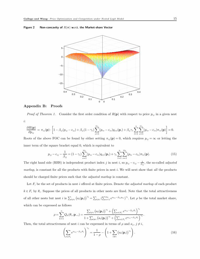
Gallego and Wang: Price Optimization and Competition under Nested Logit Model 15
Figure 2 Non-concavity of R(π) w.r.t. the Market-share Vector
00.1
0.20.3
0.4
00.1
0.20.3
0.4
−15
−10
−5
0
5
Appendix B: Proofs
Proof of Theorem 1. Consider the first order condition of R(p) with respect to price pij in a given nest
i:
∂R(p)
∂pij
= πij(p) ·[1− βij(pij − cij)+ βij(1− γi)
mi∑
s=1
(pis − cis)qs|i(pi)+ βijγi
n∑
l=1
mi∑
s=1
(pis − cis)πis(p)
]= 0.
Roots of the above FOC can be found by either setting πij(p) = 0, which requires pij = ∞ or letting the
inner term of the square bracket equal 0, which is equivalent to
pij − cij −1
βij
= (1− γi)
mi∑
s=1
(pis − cis)qs|i(pi)+ γi
n∑
l=1
ml∑
s=1
(pls − cls)πls(p). (15)
The right hand side (RHS) is independent product index j in nest i, so pij − cij − 1βij
, the so-called adjusted
markup, is constant for all the products with finite prices in nest i. We will next show that all the products
should be charged finite prices such that the adjusted markup is constant.
Let Fi be the set of products in nest i offered at finite prices. Denote the adjusted markup of each product
k ∈ Fi by θi. Suppose the prices of all products in other nests are fixed. Note that the total attractiveness
of all other nests but nest i is∑
l6=i
(al(pl)
)γl =∑
l6=i (∑ml
s=1 eαls−βlspls)γl . Let ρ be the total market share,
which can be expressed as follows
ρ =
n∑
k=1
Qk(θi,p−i) =
∑l6=i
(al(pl)
)γl +(∑
s∈Fieαis−βisθi
)γi
1 +∑
l6=i
(al(pl)
)γl +(∑
s∈Fieαis−βisθi
)γi.
Then, the total attractiveness of nest i can be expressed in terms of ρ and aj, j 6= i,(∑
s∈Fi
eαis−βisθi
)γi
=1
1− ρ−(
1 +∑
l6=i
(al(pl)
)γl
). (16)

16 Gallego and Wang: Price Optimization and Competition under Nested Logit Model
Given that the total market share is ρ and the offered product set in nest i is Fi, the adjusted markup is the
unique solution to equation (16), denoted by θFii . The total profit can be expressed as follows
RFi(ρ) = Qi(θFii ,p−i)(θ
Fii + wi(θ
Fii ))+
∑
j 6=i
Qj(θFii ,p−i)
mj∑
s=1
(pjs − cjs)qs|j(pj)
=
(1− (1− ρ)
(1 +
∑
l6=i
(al(pl)
)γl
))(θFi
i +
∑s∈Fi
eαis−βisθFii /βis
(1/(1− ρ)− (1 +
∑l6=i
(al(pl)
)γl))1/γi
)
+(1− ρ)∑
l6=i
(al(pl)
)γl
mj∑
s=1
(pjs − cjs)qs|j(pj).
Let HFi(θi) be the RHS of the above equation with θFii replaced by a free variable θi, i.e.,
HFi(θi) =
(1− (1− ρ)
(1 +
∑
l6=i
(al(pl)
)γl
))(θFi
i +
∑s∈Fi
eαis−βisθFii /βis
(1/(1− ρ)− (1 +
∑l6=i
(al(pl)
)γl))1/γi
)
+(1− ρ)∑
l6=i
(al(pl)
)γl
mj∑
s=1
(pjs − cjs)qs|j(pj). (17)
Considering its derivative at θi = θFii results in
∂HFi(θi)
∂θi
∣∣∣∣θi=θ
Fii
=
(1− (1− ρ)
(1 +
∑
l6=i
(al(pl)
)γl
))(1−
∑s∈Fi
eαis−βisθi
(1/(1− ρ)− (1 +
∑l6=i
(al(pl))γl))1/γi
)∣∣∣∣∣θi=θ
Fii
= 0.
The second equality holds because of equation (16). Recalling that HFi(θi) is convex in θi, RFi(ρ) is the
minimum of HFi(θi) with respect to θi, i.e., RFi(ρ) = minθiHFi(θi) = HFi(θFi
i ).
Suppose that another product z is added to set Fi and denote F+i := Fi ∪ z. We will next show that
RF+
i (ρ) > RFi(ρ) for any 0 < ρ < 1. Similarly, we have RF+
i (ρ) = minθiHF+
i (θi) = HF+
i (θF+
ii ), where HF+
i (θi)
is defined in function (25) and θF+
ii is the unique solution to equation (16) corresponding to offer set F+
i .
It is apparent that HF+
i (θi) > HFi(θi) for any θi. Then,
RF+
i (ρ) = HF+
i (θF+
ii ) > HFi(θ
F+
ii ) > HFi(θFi
i ) = RFi(ρ).
The second inequality holds because θFii is the minimizer of HFi(θi) with respect to θi. Therefore, RFi(ρ) is
strictly increasing in Fi for any 0 < ρ < 1 and it is optimal to offer all the products at prices such that the
adjusted markup is constant in each nest.
Lemma 1 Define wi(θi) =∑mi
k=11
βik· qk|i(θi) and vi(θi) =
∑mi
k=1 βik · qk|i(θi). The following monotonic prop-
erties hold.
(a) wi(θi) is increasing in θi and 1maxs βis
≤wi(θi)≤ 1mins βis
.
(b) vi(θi) is decreasing in θi and mins βis ≤ vi(θi) ≤maxs βis. Furthermore, wi(θi)vi(θi)≥ 1 for any θi, and
all the inequalities become equalities when βis is identical for all s∈Fi.

Gallego and Wang: Price Optimization and Competition under Nested Logit Model 17
Proof of Lemma 1. (a) Consider the first order derivative of wi(θi). Then
∂wi(θi)
∂θi
=−1 +
∑mi
k=1 eeαik−βikθi/βik
∑mi
s=1 βiseeαis−βisθi
(∑mi
s=1 eeαis−βisθi)2 .
That ∂wi(θi)∂θi
≥ 0 can be shown by Cauchy-Schwarz inequality that is∑m
i=1 xi
∑m
i=1 yi ≥(∑m
i=1
√xiyi
)2
for any xi, yi ≥ 0. Because
mi∑
k=1
eeαik−βikθi
maxs βis
≤mi∑
k=1
eeαik−βikθi
βik
≤mi∑
k=1
eeαik−βikθi
mins βis
then, 1maxs βis
≤ wi(θi) ≤ 1mins βis
and the inequalities become equalities when βis is constant for all
s = 1, . . . ,mi.
(b) Consider the first order derivative of vi(θi). Then
∂vi(θi)
∂θi
=−∑mi
k=1 β2ikeeαik−βikθi ·
∑mi
s=1 eeαis−βisθi +(∑mi
s=1 βiseeαis−βisθi
)2
(∑mi
s=1 eeαis−βisθi)2 .
It can be shown that ∂vi(θi)
∂θi≤ 0 by a similar argument to part (a).
wi(θi)vi(θi) =
∑mi
k=1 eeαik−βikθi/βik
∑mi
s=1 βiseeαis−βisθi
(∑mi
s=1 eeαis−βisθi)2 =
∂wi(θi)
∂θi
+ 1≥ 1
The inequality holds because of part (a).
Proof of Theorem 2. For the general NL model with product-differentiated price-sensitivity parameters,
the FOC of the total profit R(θ) is
∂R(θ)
∂θi
= γiQi(θ)vi(θi)
[n∑
l=1
Ql(θ)(θl + wl(θl))−(
θi + (1− 1
γi
)wi(θi)
)]= 0.
Again, because vi(θi)≥mins βis > 0, the solutions to the above FOC can be found by either letting Qi(θ) = 0,
which requires θi =∞ or setting the inner term of the square bracket equal to zero, which is equivalent to
θi + (1− 1
γi
)wi(θi) =
n∑
l=1
Ql(θ)(θl + wl(θl)). (18)
The RHS of equation (18) is independent of nest index i, so θi + (1− 1γi
)wi(θi) is invariant for each nest i,
denoted by φ. We will next show that each nest should be charged finite adjusted markup and the so-called
adjusted nest-level markup θi + (1− 1γi
)wi(θi) is constant all the nests.
Let E be the set of nests whose adjusted markup satisfies equation (18). The total market share can be
expressed as follows
ρ =∑
i∈E
Qi(θ) =
∑i∈E
(∑mi
s=1 eeαis−βisθi
)γi
1 +∑
i∈E(∑mi
s=1 eeαis−βisθi)γi
, (19)

18 Gallego and Wang: Price Optimization and Competition under Nested Logit Model
Then,
∑
i∈E
(mi∑
s=1
eeαis−βisθi
)γi
=ρ
1− ρ, (20)
θi + (1− 1
γi
)wi(θi) = φ, ∀i∈E. (21)
The solution to (20) and (21) is unique, which will be shown later, denoted by φE and θE = (θE1 , . . . , θE
n ).
The total profit can be expressed
RE(ρ) =∑
i∈E
Qi(θE)(θE
i + wi(θEi ))=∑
i∈E
Qi(θE)
(φE +
wi(θEi )
γi
)
= ρφE +∑
i∈E
(∑mi
s=1 eeαis−βisθEi
)γi
·wi(θEi )
γi/(1− ρ),
Define a new function HE(φ) with φE replaced by a free variable φ but keeping the relation between φ and
θi as shown in (21), i.e.,
HE(φ) = ρφ+∑
i∈E
(∑mi
s=1 eeαis−βisθi
)γi ·wi(θi)
γi/(1− ρ). (22)
where θi satisfies (21) for each i ∈ E. We will next show that HE(φ) is convex in φ under Condition 1 for
each i.
∂HE(φ)
∂φ= ρ +
∑
i∈E
∂GE(φ)/∂θi
∂φ/∂θi
= ρ− (1− ρ)∑
i∈E
(mi∑
s=1
eeαis−βisθi
)γi
,
where GE(φ) =∑
i∈E
(Pmi
s=1eeαis−βisθi)
γi ·wi(θi)
γi/(1−ρ). The second equality holds because
∂GE(φ)
∂θi
= −1− ρ
γi
·(1− (1− γi)wi(θi)vi(θi)
)(
mi∑
s=1
eeαis−βisθi
)γi
,
∂φ
∂θi
=1
γi
(1− (1− γi)wi(θi)vi(θi)
).
Moreover,
∂HE(φ)
∂φ
∣∣∣∣φ=φE
= 0.
The above equality holds because of equation (20). The second order derivative of HE(φ) is
∂2HE(φ)
∂φ2=∑
i∈E
∂∂θi
(∂HE(φ)/∂φ)
∂φ/∂θi
=∑
i∈E
γ2i (1− ρ)vi(θi)
(∑mi
s=1 eeαis−βisθi
)γi
1− (1− γi)wi(θi)vi(θi)> 0.
The inequality holds because 1− (1− γi)wi(θi)vi(θi) > 0 under Condition 1.
Thus, HE(φ) is convex in φ, and the solution to (20) and (21) is unique. Moreover, RE(ρ) is the minimum
of HE(φ) with respect to φ, i.e., RE(ρ) = minφ HE(φ). Let E+ be the new nest set if the adjusted markup of
another nest satisfies equation (18). We will next show that RE+
(ρ) > RE(ρ) for any 0 < ρ < 1.

Gallego and Wang: Price Optimization and Competition under Nested Logit Model 19
It is apparent that HE+
(φ) > HE(φ) for any φ, where HE+
(φ) is the function defined in (22) corresponding
to offer set E+. Then,
RE+
(ρ) = HE+
(φE+
) > HE(φE+
) > HE(φE) = RE(ρ).
The second inequality holds because φE is the minimizer of HE(φ). Therefore, RE(ρ) is strictly increasing
in E for any 0 < ρ < 1 and it is optimal to offer all the products at prices such that the adjusted nest-level
markup is constant for all the nests.
Proof of Coronary 1. Consider the FOC of R(φ),
∂R(φ)
∂φ=
n∑
i=1
∂R(θ)/∂θi
∂φ/∂θi
= (R(φ)−φ)
n∑
i=1
γ2i Qi(θ)vi(θi)
1− (1− γi)wi(θi)vi(θi)= 0, (23)
where θi is the solution to equation (21). Because∑n
i=1
γ2i Qi(θ)vi(θi)
1−(1−γi)wi(θi)vi(θi)> 0 under Condition 1 for each i,
then, R(φ) is increasing (decreasing) in φ if and only if R(φ)≥ (≤)φ.
(i) Case I: there is only one solution to equation (23), denoted by φ∗. Apparently R(φ) is increasing in φ
for φ≤ φ∗ and is decreasing in φ for φ > φ∗.
(ii) Case II: there are multiple solutions to equation (23). Suppose that there are two consecutive solutions
φ1 = R(φ1) < φ2 = R(φ2) and there is no solution to equation (23) between φ1 and φ2. It must hold that
R(φ) < R(φ2) for any φ1 < φ < φ2; otherwise, there must be another solution to equation (23) between
φ1 and φ2, which contradicts that φ1 and φ2 are two consecutive solutions. We claim that R(φ) is
increasing in φ for φ∈ [φ1, φ2]. Assume there are two points φ1 < φ′1 < φ′
2 < φ2 such that R(φ′1) > R(φ′
2).
Then, there must be a solution to equation (23) between φ′1 and φ2, which also contradicts that φ1 and
φ2 are two consecutive solutions. Thus, R(φ) is increasing between any two solutions to equation (23)
and R(φ) may be decreasing after the largest solution. Therefore, R(φ) is unimodual with respect to φ
under Condition 1.
Proof of Coronary 2. Let ρ(φ) =∑n
i=1 Qi(θ), where θi is the solution to θi + (1− 1γi
)wi(θi) = φ, for each
i = 1,2, . . . , n. Then,
∂ρ(φ)
∂φ=
n∑
i=1
∂ρ(φ)/∂θi
∂φ/∂θi
=−Q0(θ)n∑
i=1
γ2i Qi(θ)vi(θi)
1− (1− γi)wi(θi)vi(θi),
∂R(φ)
∂ρ=
∂R(φ)/∂φ
∂ρ(φ)/∂φ=−R(θ)−φ
1− ρ.
We can easily show that R(ρ) is unimodual in ρ by a similar argument to part (c). Moreover, we consider
the second order derivative under Condition 1 for all i,
∂2R(ρ)
∂ρ2= − ∂
∂ρ· R(θ)−φ
1− ρ=−R(θ)−φ
(1− ρ)2+
1
1− ρ·
∂R(θ)
∂φ− 1
∂ρ
∂φ

20 Gallego and Wang: Price Optimization and Competition under Nested Logit Model
= − 1
(1− ρ)2∑n
i=1
γ2i
Qi(θ)vi(θi)
1−(1−γi)wi(θi)vi(θi)
< 0.
The last equality hold because (1 − γi)wi(θi)vi(θi) < 1 for all θi and each i under Condition 1. Therefore,
R(ρ) is concave in ρ under Condition 1.
Proof of Theorem 3. (a) Suppose that (p∗i ,p
∗−i) is an equilibrium of Game I. From Theorem 1, the
adjusted markup is constant for all the products of each firm, i.e., pij − cij − 1βij
is constant for all j,
denoted by θ∗i . We will argue that (θ∗
i , θ∗−i) must be the equilibrium of Game II. If firm i is better-off
to deviate to θi, then firm i will also be better-off to deviate to pi in Game I, where pi = (pi1, . . . , pimi)
and pij = θi + cij + 1βij
. It contradicts that (p∗i ,p
∗−i) is an equilibrium of Game I.
Suppose that (θ∗i , θ∗
−i) is an equilibrium of Game II. We will argue that (p∗i ,p
∗−i) is an equilibrium of
Game I, where pij = θ∗i + cij + 1
βijfor each j. If firm i is better-off to deviate to pi := (pi1, pi2, . . . , pimi
)
in Game I, pij − cij − 1βij
must be constant for each j by Theorem 1, denoted by θi. Then, firm i must
be better-off to deviate to θi in Game II, which contradicts that (θ∗i , θ∗
−i) is an equilibrium of Game
II.
(b) Consider the derivatives of logRi(θi, θ−i):
∂ logRi(θi, θ−i)
∂θi
= −γi(1−Qi(θi, θ−i))vi(θi)+wi(θi)vi(θi)
θi + wi(θi),
∂ logRi(θi, θ−i)
∂θj
= γjQj(θj , θ−j)vj(θj)≥ 0, ∀j 6= i,
∂2 logRi(θi, θ−i)
∂θi∂θj
= γiγjQi(θi, θ−i)Qj(θj , θ−j)vi(θi)vj(θj)≥ 0, ∀j 6= i.
Then, Game II is a log-supermodular game. Note that the strategy space for each firm is the real line.
From Topkis (1998) and Vives (2001), the equilibrium set is a nonempty complete lattice and, therefore,
has the componentwise largest element θ∗
and smallest element θ∗, respectively.
For any equilibrium θ∗, it holds that θ∗ ≥ θ∗ ≥ θ∗ and
logRi(θ∗i , θ
∗−i)≤ logRi(θ
∗i , θ
∗
−i)≤ logRi(θ∗
i , θ∗
−i).
The first inequality holds because ∂ logRi(θi, θ−i)/∂θj ≥ 0; the second inequality holds because (θ∗
i , θ∗
−i)
is a Nash equilibrium. Because logarithm is a monotonic increasing transformation, then
Ri(θ∗i , θ∗
−i)≤Ri(θ∗i , θ
∗
−i)≤Ri(θ∗
i , θ∗
−i).
Therefore, the largest equilibrium θ∗
is preferred by all the firms.

Gallego and Wang: Price Optimization and Competition under Nested Logit Model 21
Proof of Theorem 4 (a) Suppose that there exists an asymmetric equilibrium, denoted by
(θ∗1, θ
∗2, θ
∗3, . . . , θ
∗n). Suppose that θ∗
1 is the largest and θ∗2 is the smallest without loss of generality, then
θ∗1 > θ∗
2. Because the game is symmetric, (θ∗2, θ
∗1, θ
∗3, . . . , θ
∗n) is also an equilibrium. In other words, the best
strategies for firm 1 are θ∗1 and θ∗
2 respectively corresponding to other firms’ strategies (θ∗2, θ
∗3, . . . , θ
∗n)
and (θ∗1, θ
∗3, . . . , θ
∗n). Since the game is strictly supermodular and (θ∗
2, θ∗3, . . . , θ
∗n) < (θ∗
1, θ∗3, . . . , θ
∗n), then
θ∗1 ≤ θ∗
2, which contradicts that θ∗1 > θ∗
2.
(b) Consider the derivative of Ri(θi, θ−i) with respect to θi as follows:
∂Ri(θi, θ−i)
∂θi
= −γiQi(θi, θ−i)(1−Qi(θi, θ−i)
)vi(θi)
[θi +
(1− 1
γi(1−Qi(θi, n))
)wi(θi)
].
Define Y (θi) as follows:
Y (θi) = θi +
(1− 1
γi(1−Qi(θi, n))
)wi(θi).
Its derivative can be expressed by
∂Y (θi)
∂θi
=1
γi(1−Qi(θi, n))·(
1−wi(θi)vi(θi)
(1− γi + γi
(n− 1)(Qi(θi, n))2
1−Qi(θi, n)
)),
Clearly, Qi(θi, n), the probability to select nest i if all firms charge the same adjusted markup θi, is less
than 1/n, i.e., Qi(θi, n) < 1n. Then,
∂Y (θi)
∂θi
>1
γi(1−Qi(θi, n))·(
1−wi(θi)vi(θi)
(1− n− 1
nγi
)).
Therefore,
(i) If γi ≥ nn−1
, then ∂Y (θi)
∂θi> 0 for any θi.
(ii) If 0 < γi < nn−1
and maxs βis
mins βis≤ 1
1−n−1
n·γi
, we claim that wi(θi)vi(θi)(1− n−1
nγi
)< 1. If there are more
than one products with different price coefficients, wi(θi)vi(θi) < maxs βis
mins βis; otherwise wi(θi)vi(θi) = 1
for any θi. In both cases, wi(θi)vi(θi)(1− n−1
nγi
)< 1.
Thus, ∂Y (θi)
∂θi> 0 for any θi under Condition 2. Then, Y (θi) is strictly increasing from negative to positive
as θi goes from −∞ to ∞. Hence, there exists a unique solution to the equation Y (θi) = 0 and it is also
the unique equilibrium to the symmetric game.
Proof of Theorem 5. Similar to the proof of Theorem 1, consider the FOC for the profit R(p) under the
Nested Attraction model:
∂R(p)
∂pij
=πij(p)a′
ij(pij)
βijaij(pij)·[(pij − cij)+
aij(pij)
a′ij(pij)
− (1− γi)
mi∑
s=1
(pis − cis)qs|i(pi)− γi
n∑
l=1
mi∑
s=1
(pis − cis)πis(p)
]= 0.

22 Gallego and Wang: Price Optimization and Competition under Nested Logit Model
The above equation is satisfied when eitherβijπij(p)a′
ij(pij)
aij(pij)= 0, which requires a′
ij(pij) = 0, or the inner term
of the square bracket is equal to zero, i.e.,
(pij − cij)+aij(pij)
a′ij(pij)
= (1− γi)
mi∑
s=1
(pis − cis)qs|i(pi)+ γi
n∑
l=1
mi∑
s=1
(pis − cis)πis(p). (24)
We remark that the RHS of (24) is independent of product index j, so (pij − cij) +aij(pij)
a′
ij(pij)
is invariant in
products of set Fi in nest i, where Fi is the offer set of products in nest i at prices such that equation (24)
is satisfied. Denote θFii = (pij − cij)+ aij(pij)/a′
ij(pij) for each product j in set Fi.
Suppose that the prices of all other nests are fixed. Consider the price optimization problem with the
market share constraint as follows:
RFi(ρ,p−i) := maxpij<∞,∀j∈Fi
∑l6=i
∑ml
s=1(pls − cls)πls(pi,p−i)+∑
k∈Fi(pik − cik)πik(pi,p−i)
s.t., Qi(pi,p−i) = ρ.
Let al =∑ml
s=1 als(pls) for each l 6= i for the ease of notation. After some algebra, the total market share
constraint Qi(pi,p−i) = ρ results in
∑
s∈Fi
ais(pis) =
(ρ
1− ρ−∑
l6=i
aγl
l
)1/γi
.
Then, RFi(ρ,p−i) can be rewritten as follows
RFi(ρ,p−i) =
(ρ− (1− ρ)
∑
l6=i
aγl
l
)·(
θFii −
(ρ/(1− ρ)−
∑
l6=i
aγl
l
)−1/γi∑
s∈Fi
(ais(pis))2
a′is(pis)
)+∑
l6=i
(1− ρ)aγl
l
ml∑
s=1
(pls − cls)qs|l(pl),
where pis is uniquely determined by (pis − cis)+ ais(pis)/a′is(pis) = θFi
i for each s∈Fi.
Define function HFi(θi) as follows
HFi(θi) = θi −(ρ/(1− ρ)−
∑
l6=i
aγl
l
)−1/γi∑
s∈Fi
(ais(pis))2
a′is(pis)
, (25)
where pis is uniquely determined by (pis − cis)+ais(pis)/a′is(pis) = θi for each s∈ Fi. Consider the first order
derivative for function HFi(θi):
∂HFi(θi)
∂θi
= 1−(ρ/(1− ρ)−
∑
l6=i
aγl
l
)−1/γi∑
s∈Fi
∂∂pis
(ais(pis))2
a′
is(pis)
∂θi/∂pis
= 1−(ρ/(1− ρ)−
∑
l6=i
aγl
l
)−1/γi∑
s∈Fi
2ais(pis)(a′
is(pis))2−(ais(pis))2a′′
is(pis)
(a′
is(pis))2
1 +(a′
is(pis))2−ais(pis)a′′
is(pis)
(a′
is(pis))2
= 1−(ρ/(1− ρ)−
∑
l6=i
aγl
l
)−1/γi∑
s∈Fi
ais(pis).
Then, it follows that
∂HFi(θi)
∂θi
∣∣∣∣θi=θ
Fii
= 0.

Gallego and Wang: Price Optimization and Competition under Nested Logit Model 23
The equality holds because∑
s∈Fiais(pis) =
(ρ
1−ρ−∑
l6=iaγl
l
)1/γi
. The second order derivative of HFi(ηi) is
∂2HFi(θi)
∂θ2i
=∑
s∈Fi
∂∂pis
(∂HFi(θi)/∂θi)∂θi
∂pis
=−(ρ/(1− ρ)−
∑
l6=i
aγll
)−1/γi∑
s∈Fi
(a′is(pis))
3
2(a′is(pis))2 − ais(pis)a′′
is(pis)≥ 0.
The inequality holds because a′is(pis) ≤ 0 and 2(a′
is(pis))2 − ais(pis)a
′′is(pis) > 0 from Condition 3. Thus,
HFi(θi) is convex in θi and RFi(ρ,p−i) = minθiHFi(θi) = HFi(θFi
i ).
Suppose that another product z is added to set Fi and denote F+i := Fi ∪z. Similarly, we have RF+
i (ρ) =
minθiHF+
i (θi) = HF+
i (θF+
ii ), where HF+
i (θi) is defined in function (25) and θF+
ii is the unique solution to
equation (16) corresponding to offer set F+i . It is apparent that HF+
i (θi) > HFi(θi) for any θi. Then,
RF+
i (ρ) = HF+
i (θF+
ii ) > HFi(θ
F+
ii ) > HFi(θFi
i ) = RFi(ρ).
Therefore, it is optimal to offer all the products in nest i, i.e., Fi = 1,2, . . . ,mi. Moreover, their prices
satisfy that (pij − cij)+aij(pij)
a′
ij(pij)
is constant for all the products in nest i.
Appendix C: Uniqueness of the Nash Equilibrium
In this section, we will investigate the uniqueness of the Nash equilibrium in the general case. First, we state
sufficient conditions.
Condition 4 (a) Denote Ψ as the region such that
−∂Qi(θi, θ−i)
∂θi
>∑
j 6=i
∂Qi(θi, θ−i)
∂θj
, θ ∈Ψ, i = 1,2, . . . , n.
(b) Denote Ωi as the region such that θi + wi(θi) is log-concave in θi ∈Ωi, i = 1,2, . . . , n.
Notice that the NL model with product-differentiated price-sensitivity parameters within a nest and homo-
geneous nest coefficients, satisfies Condition 4 for any θ. Condition 4(a) is a standard diagonal dominant
condition (see e.g., Vives 2001) and it says that a uniform increase of the adjusted markups by all the firms
would result in a decrease of any firm’s market share. In the NL model, Condition 4(a) is equivalent to
γivi(θi) >n∑
j=1
γjQj(θj , θ−j)vj(θj). (26)
From Lemma 1, inequality (26) can be implied by the following condition that is stronger but easier to be
verified:
mini
γi minl,s
βl,s > maxi
γi maxl,s
βl,s
n∑
j=1
Qj(θj , θ−j),

24 Gallego and Wang: Price Optimization and Competition under Nested Logit Model
which is equivalent to
n∑
l=1
(ml∑
s=1
eeαls−βlsθl
)γl
<mini γi minl,s βls
maxi γi maxl,s βls −mini γi minl,s βls
. (27)
From inequalition (27), Condition 4(b) can be satisfied when the adjusted markups θi are sufficiently large
for all the firms.
Apparently, θi + wi(θi) > 0 because each firm sells all her products at a positive average margin. Then,
Condition 4(b) can be implied by a stronger condition that θi + wi(θi) or wi(θi) is concave in θi for each
i = 1,2, . . . , n because if wi(θi) is concave, then
∂2 log(θi + wi(θi))
∂θ2i
=w′′
i (θi)(θi + wi(θi))− (w′i(θi))
2
(θi + wi(θi))2≤ 0,
where w′i(θi) = ∂wi(θi)/∂θi and w′′
i (θi) = ∂2wi(θi)/∂θ2i .
When θi is large enough, Condition 4(b) can also be satisfied without requiring the concavity of θi +wi(θi)
or wi(θi).
Lemma 2 There exist a threshold θi for each firm i such that θi + wi(θi) is log-concave in θi for θi ≥ θi.
Proof of Lemma 2. Consider the derivatives of log(θi + wi(θi)),
∂ log(θi + wi(θi))
∂θi
=wi(θi)vi(θi)
θi + wi(θi),
∂2 log(θi + wi(θi))
∂θ2i
=wi(θi)
θi + wi(θi)· ∂vi(θi)
∂θi
+ vi(θi) ·∂ wi(θi)
θi+wi(θi)
∂θi
=wi(θi)
θi + wi(θi)· ∂vi(θi)
∂θi
+ vi(θi) ·θi ·(− 1 + wi(θi)vi(θi)
)−wi(θi)
(θi + wi(θi))2
The log-concavity of θi + wi(θi) can be guaranteed by θi ·(− 1 + wi(θi)vi(θi)
)−wi(θi) ≤ 0 because vi(θi) is
decreasing from Lemma 1. We will next show that θi ·(−1+wi(θi)vi(θi)
)→ 0 as θi →∞. Denote β
i= mins βis
and let Ξi be the set Ξi = s : βis = βi. Then,
−1 + wi(θi)vi(θi) =−(∑mi
s=1 eeαis−βisθi
)2+(∑mi
s=11
βiseeαis−βisθi
)·(∑mi
s=1 βiseeαis−βisθi
)
(∑mi
s=1 eeαis−βisθi)2
=1
(∑s∈Ξi
eeαis +∑
s/∈Ξieeαis−(βis−β
i)θi
)2 ·(−(∑
s∈Ξi
eeαis +∑
s/∈Ξi
eeαis−(βis−βi)θi
)2
+
(∑
s∈Ξi
1
βi
eeαis +∑
s/∈Ξi
1
βis
eeαis−(βis−βi)θi
)·(∑
s∈Ξi
βieeαis +
∑
s/∈Ξi
βiseeαis−(βis−β
i)θi
))
≈
∑s∈Ξi
eeαis ·(∑
s/∈Ξi(βis
βi
+β
i
βis− 2)eeαis−(βis−β
i)θi
)
(∑s∈Ξi
eeαis
)2
+ 2(∑
s∈Ξieeαis
)·(∑
s/∈Ξieeαis−(βis−β
i)θi
)

Gallego and Wang: Price Optimization and Competition under Nested Logit Model 25
In the above approximation, the higher order terms are ignored. Because βis
βi
+β
i
βis− 2 > 0 and βis − β
i> 0,
then
θi ·((βis
βi
+β
i
βis
− 2)eeαis−(βis−β
i)θi
)=
θi ·(
βis
βi
+β
i
βis− 2)
e−eαis+(βis−βi)θi
→ 0, as θi →∞.
The above convergence holds because the exponential function is increasing faster than the linear function.
Since(∑
s∈Ξieeαis
)2
+2(∑
s∈Ξieeαis
)·(∑
s/∈Ξieeαis−(βis−β
i)θi
)→(∑
s∈Ξieeαis
)2
as θi →∞, therefore, θi ·(−
1 + wi(θi)vi(θi))→ 0. There exists θi such that
θi ·(− 1 + wi(θi)vi(θi)
)≤ 1
maxs βis
≤wi(θi), for θi ≥ θi.
Thus, θi + wi(θi) is log-concave for θi ≥ θi.
Tatonnement process can reach equilibrium under some mild conditions. In the basic tatonnement process,
firms take turns in adjusting their price decisions and each firm reacts optimally to all other firms’ prices
without anticipating others’ response, which can be interpreted as a way of expressing bounded rationality
of agents. In each iteration, firms respond myopically to the choices of other firms in the previous iteration
and the dynamic process can be expressed below.
Tatonnement Process: Select a feasible vector θ(0); in the kth iteration determine the optimal response
for each firm i as follows:
θ(k)i = arg max
θi∈Ωi∩ΨRi(θi, θ
(k−1)−i ). (28)
Theorem 6 Suppose θ∗ is an equilibrium under Condition 4,
(a) θ∗ is the unique pure Nash equilibrium of Game II in region (
⋂n
i=1 Ωi)⋂
Ψ.
(b) The unique pure Nash equilibrium θ∗ can be computed by the tatonnement scheme, starting from an
arbitrary price vector θ(0) in the region (⋂n
i=1 Ωi)⋂
Ψ, i.e., θ(k) converges to θ∗.
Proof of Theorem 6. Consider the first order and second order derivatives of logRi(θi, θ−i) with respect
to θi:
∂ logRi(θi, θ−i)
∂θi
=∂ log(Qi(θi, θ−i))
∂θi
+∂ log(θi + wi(θi))
∂θi
=−γi(1−Qi(θi, θ−i))vi(θi)+∂ log(θi + wi(θi))
∂θi
,
∂2 logRi(θi, θ−i)
∂θ2i
= −γ2i Qi(θi, θ−i)(1−Qi(θi, θ−i))
(vi(θi)
)2+
∂2 log(θi + wi(θi))
∂θ2i
.
The cross-derivative of logRi(θi, θ−i) is
∂2 logRi(θi, θ−i)
∂θi∂θj
= γiγjQi(θi, θ−i)Qj(θj, θ−j)vi(θi)vj(θj)≥ 0, ∀j 6= i.

26 Gallego and Wang: Price Optimization and Competition under Nested Logit Model
Then,
∑
j 6=i
∂2 logRi(θi, θ−i)
∂θi∂θj
= γiQi(θi, θ−i)vi(θi)∑
j 6=i
γjQj(θj , θ−j)vj(θj).
Under Condition 4, Ri(θi, θ−i) is log-dominant diagonal,
−∂2 logRi(θi, θ−i)
∂θ2i
≥∑
j 6=i
∂2 logRi(θi, θ−i)
∂θi∂θj
(29)
The inequality holds because
γ2i Qi(θi, θ−i)(1−Qi(θi, θ−i))
(vi(θi)
)2 ≥ γiQi(θi, θ−i)vi(θi)∑
j 6=i
γjQj(θj , θ−j)vj(θj)
under Condition 4(a), and
∂2 log(θi + wi(θi))
∂θ2i
≤ 0
under Condition 4(b). The inequality (29) establishes the uniqueness of the Nash equilibrium to Game II
(see e.g., Vives 2001).
If the equilibrium of a log-supermodular game with continuous payoff is unique, it is globally stable and a
tatonnement process with dynamic response (28) converges to it from any initial point in the feasible region.
References
Akcay, Y., H. P. Natarajan, S. H. Xu. 2010. Joint dynamic pricing of multiple perishable products under
consumer choice. Management Sci. 56(8) 1345 – 1361.
Allon, G., A. Federgruen, M. Pierson. 2011. Price competition under multinomial logit demand functions
with random coecients. Working paper, Northwestern University.
Anderson, S. P., A. de Palma. 1992. Multiproduct firms: A nested logit approach. The Journal of Industrial
Economics, 40(3) 261–276.
Anderson, S. P., A. de Palma, J. Thisse. 1992. Discrete Choice Theory of Product Differentiation. 1st ed.
The MIT Press.
Aydin, G., E. L. Porteus. 2008. Joint inventory and pricing decisions for an assortment. Oper. Res. 56(5)
1247–1255.
Aydin, G., Jennifer K. Ryan. 2000. Product line selection and pricing under the multinomial logit choice
model. Working paper.

Gallego and Wang: Price Optimization and Competition under Nested Logit Model 27
Bernstein, F., A. Federgruen. 2004. A general equilibrium model for industries with price and service
competition. Oper. Res. 52(6) 868–886.
Berry, S., J. Levinsohn, A. Pakes. 1995. Automobile prices in market equilibrium. Econometrica 63(4)
841–890.
Borsch-Supan, A. 1990. On the compatibility of nested logit models with utility maximization. Journal of
Econometrics 43 373–388.
Cachon, G. P., A. G. Kok. 2007. Category management and coordination in retail assortment planning in
the presence of basket shopping consumers. Management Sci. 53(6) 934 – 951.
Corless, R. M., G. H. Gonnet, D. E. G. Hare, D. J. Jeffrey, D. E. Knuth. 1996. On the Lambert W function.
Advances in Computational Mathematics 5(1) 329–359.
Daganzo, C. R., M. Kusnic. 1993. Two properties of the nested logit model. Transportation Science 27(4)
395–400.
Debreu, G. 1952. A social equilibrium existence theorem. Proceedings of the National Academy of Sciences
38(10) 886–93.
Dong, L., P. Kouvelis, Z. Tian. 2009. Dynamic pricing and inventory control of substitute products. Manu-
facturing Service Oper. Management 11(2) 317–339.
Erdem, T., J. Swait, Louviere. 2002. The impact of brand credibility on consumer price sensitivity. Inter-
national Journal of Research in Marketing 19(1) 1–19.
Federgruen, A., N. Yang. 2009. Competition under generalized attraction models: Applications to quality
competition under yield uncertainty. Management Sci. 55(12) 2028–2043.
Gallego, G., W. T. Huh, W. Kang, R. Phillips. 2006. Price competition with the attraction demand model:
Existence of unique equilibrium and its stability. Manufacturing Service Oper. Management 8(4) 359–
375.
Gallego, G., C. Stefanescu. 2011. Upgrades, upsells and pricing in revenue management. Working paper,
Columbia University.
Greene, W. H. 2007. Econometric Analysis . Pearson Education.
Hanson, W., K. Martin. 1996. Optimizing multinomial logit profit functions. Management Sci. 42(7) 992–
1003.
28 Gallego and Wang: Price Optimization and Competition under Nested Logit Model
Hopp, W. J., X. Xu. 2005. Product line selection and pricing with modularity in design. Management Sci.
7(3) 172–187.
Kok, A. G., Y. Xu. 2011. Optimal and competitive assortments with endogenous pricing under hierarchical
consumer choice models. Management Sci. 57(9) 1546–1563.
Li, H., W. T. Huh. 2011. Pricing multiple products with the multinomial logit and nested logit models:
Concavity and implications. Manufacturing Service Oper. Management 13(4) 549 – 563.
Liu, G. 2006. On nash equilibrium in prices in an oligopolistic market with demand characterized by a nested
multinomial logit model and multiproduct firm as nest. Discussion Papers, Statistics Norway.
Luce, R. D. 1959. Individual Choice Behavior: A Theoretical Analysis. Wiley New York.
McFadden, D. 1974. Conditional logit analysis of qualitative choice behavior. P. Zarembka, ed., Frontiers in
Econometrics . Academic Press, New York, 105–142.
McFadden, D. 1980. Econometric models for probabilistic choice among products. The Journal of Business
53(3) 13–29.
Milgrom, P., J. Roberts. 1990. Rationalizability, learning, and equilibrium in games with strategic comple-
mentarities. Econometrica: Journal of the Econometric Society 58(6) 1255–1277.
Nash, J. F. 1951. Non-coorperative games. The Annals of Mathematics 54(2) 286–295.
Song, J., Z. Xue. 2007. Demand management and inventory control for substitutable products. Working
paper, Duke University.
Topkis, D. M. 1998. Supermodularity and complementarity. Princeton University Press.
Vives, X. 2001. Oligopoly pricing: Old ideas and new tools. The MIT Press.
Williams, H. C. W. L. 1977. On the formation of travel demand models and economic evaluation measures
of user benefit. Environment and Planning 9(A) 285–344.
Williams, H. C. W. L., J. de D. Ortuzar. 1982. Behavioural theories of dispersion and the mis-specication
of travel demand models. Transportation Research 16(B) 167–219.