multi-source energy harvesting for wireless sensor nodes
TRANSCRIPT

Royal Institute of Technology (KTH)
Multi-Source Energy Harvesting for
Wireless Sensor Nodes
Kai Kang
Supervisor:
Qiang Chen & Zhibo Pang
Examiner:
Li-Rong Zheng

1
Abstract
The past few years have seen an increasing interest in the development of wireless sensor
networks. But the unsatisfactory or limited available energy source is one of the major bottlenecks
which are limiting the wireless sensor technology from mass deployment. Ambient energy
harvesting is the most promising solution towards autonomous sensor nodes by providing low cost,
permanent, and maintenance-free energy source to wireless sensor nodes. In this paper, we first
invested available energy source such as solar, vibration, thermal and other potential energy
sources, and described the mathematical model of each energy source. Secondly, a novel adaptive
topology maximum point power tracking method is proposed. This method is that changes the
solar cells array from series to parallel or series-parallel mixed way to find out a best array that
output the maximum power. This method also can be used in other energy source. At last, we
purchased the matured energy generator: vibration, thermal, and solar panels to measure and
verify the output power of each energy source. The experimental result showed that the conversion
efficiency of this novel MPPT method can reach 60%-80% in outdoor and it is able to supply
sufficient power to wireless sensor nodes.

2
Contents
Abstract ............................................................................................................................................. 1
1. Introduction and Background .................................................................................................... 4
1.1. System Architecture ...................................................................................................... 5
1.2. History ........................................................................................................................... 6
1.3. Energy Harvesting Sources ........................................................................................... 6
2. Photovoltaic (Solar Cell) ........................................................................................................... 9
2.1. Photovoltaic Model ....................................................................................................... 9
2.2. Maximum Power Point Tracking Methods ................................................................. 12
2.2.1. Constant Voltage Method ................................................................................ 13
2.2.2. Short-Current Pulse Method............................................................................ 13
2.2.3. Fractional Open-Circuit Voltage (FOCV) ....................................................... 13
2.2.4. Perturb and Observe Methods (P&O) ............................................................. 15
2.2.5. Incremental Conductance Method (IncCond) ................................................. 15
2.2.6. Comparison of MPPT Methods ........................................................................ 15
3. Thermoelectric Generator ........................................................................................................ 18
3.1. Thermoelectric Effect .................................................................................................... 18
3.2. MPPT Method ............................................................................................................... 20
4. Vibration .................................................................................................................................. 23
4.1. Methods of Converting Vibrations to Electricity .......................................................... 23
4.1.1. Electromagnetic.................................................................................................. 24
4.1.2. Electrostatic ........................................................................................................ 25
4.1.3. Piezoelectric ....................................................................................................... 26
4.1.4. Comparison of Conversion Methods .................................................................. 26
4.2. Piezoelectric Model ....................................................................................................... 28
5. Other Energy Source ................................................................................................................ 31
5.1. Human Power ................................................................................................................ 31
5.2. Wind/Air Flow .............................................................................................................. 31
5.3. Electromagnetic ............................................................................................................ 32
3
6. Energy Storage ......................................................................................................................... 33
6.1. Super Capacitor ........................................................................................................... 33
6.2. Batteries ...................................................................................................................... 34
7. Adaptive-Topology MPPT Method ......................................................................................... 35
7.1. Solar Cell Output Characteristics ................................................................................ 35
7.2. MPPT Method and Model ........................................................................................... 37
7.3. System and Control Flow ............................................................................................ 39
8. Experimental Result ................................................................................................................ 41
8.1. Thermal Generator Result ........................................................................................... 41
8.2. Vibration Result .......................................................................................................... 46
8.3. Solar Cells Array Result .............................................................................................. 48
8.4. Power Supply to MCU ................................................................................................ 57
9. Conclusion and Future Work ................................................................................................... 59
References ....................................................................................................................................... 60

4
1. Introduction and Background
The past few years have seen an increasing interest in the development of wireless sensor
networks. It is obviously that more and more wireless sensor nodes will be deployed around our
environment, such as the monitoring of human living condition, environment, animals and plants,
health monitoring of civil structures, industry control etc. In many applications, for example, an
ECG sensor is taken by a patient to monitor his heart, and a light sensor embedded in a light to
adjust light illumination.
In order to operate these sensors, some of them are able to be powered by common power
such as 220V AC power which connects to power grid or other high-power source. But under
most of circumstances, wireless sensor nodes or sensors which can hardly have physical
connections to the outside world, they must be powered by themselves or batteries. Unfortunately,
batteries have many disadvantages, included bulk size, finite energy, limited off-shelf life, and
chemical that could course environment pollution [1]. These disadvantages will increase wireless
sensor network maintain cost. Batteries must be replaced by new batteries every one or two years
because of its life. Especially in wilderness, replace new batteries is a complex task. To overcome
these disadvantages of battery, a self power, scavenging energy from ambient environment and
long life low cost power system is required in wireless sensor networks.
Owing to the limiting factor of batteries on the above disadvantages, few kinds of available
ambient energy sources such solar and vibration have been developed to supply power to wireless
sensor node. The purpose of this paper is to review existing and potential power source for
wireless sensor network and design a multi-source energy harvesting management system. This
power management system includes energy scavenging module, control module and energy
storage module.
In this paper, we would introduce the power system architecture, history of energy harvesting
in chapter 1. From chapter 2-6, we would detail study available ambient energy source, energy
reservoir, and charger. In chapter 7, we propose a novel MPPT method to optimize solar cell, this
method also can be used in other ambient source. The experimental results we be exhibited in
chapter 8. At last in chapter, we would like to conclude this paper and propose some future tasks.

5
1.1. System Architecture
In order to supply ambient environment energy to wireless sensor nodes, the power system
architecture should consist of at least three modules: an energy source, an energy reservoir, and
charge controller. As shown in Fig. 1.1, this is the fundamental power system architecture. It
includes an ambient energy source, an energy reservoir module (battery and buffer), and charge
controller (MCU and switch).
Ambient Energy Source
Buffer (Super Capacitor)
SwitchWirelessSensor Nodes
Battery
Charging Controller (MCU)
Fig. 2.1 System Architecture
Ambient energy source, typically defined as power generator. This module consists of some
power generators and a maximal power point tracking (MPPT) circuits. The generator converts
ambient energy source such as solar, mechanical energy, air flow, thermal etc. to electrical energy.
The conversion ability depends on the ambient energy source density, the generator size and
production technology. In order to maximize conversion, a MPPT circuit is necessary and
controlled by charging controller or MCU. The MPPT method varies from different ambient
energy source.
Buffer and battery are two important parts of energy reservoir module. Buffers are typically
capacitor, super capacitor. These buffers collect energy from power generator and supply power to
charging controller. They also charge the battery if the collected power is larger than consumed
power. Battery supply energy to system when collected power is less than consumed power.
Charge controller is always a micro controller unit (MCU) which is powered by buffer or

6
battery, it controls the MPPT circuit to maximize the conversion efficiency of power generator and
switch between buffers and battery.
1.2. History
The first observation of energy harvesting in form of current from ambient natural source was
in 1826 when Thomas Johann Seebeck found that it occur a current flow in a closed circuit made
of two different metals when the temperature is different in these two metals [2][3]. In the
following decade years, thermoelectric effects were explored and power generation, and
refrigeration was recognized [4].
In 1831, Joseph Henry and Michael Faraday discovered electromagnetic induction that
produced electricity from magnetism [7]. In October of this year, the first direct-current generator
which consisting of a copper plate rotating between magnetic poles was invented by Michael
Faraday [8].
Edmund Becquerel discovered the photovoltaic effect in 1839 [5], and Charles Fritts coated a
layer of selenium with a thin layer of gold and constructed the first large area solar cell in 1894 [6].
It had a higher efficiency while after developing the quantum theory of light and solid state
physics in the early 1900s [5].
Pieere and Jacques Curie predicted and proved experimentally piezoelectricity in 1880,
which is a phenomenon that certain crystals would exhibit a surface charge when subject to
mechanical stress [2].
1.3. Energy Harvesting Sources
Ambient environment exist a large number of energy, such as solar, air flow, thermal energy
and so on, but these are unlike to fossil fuel or nuclear fuel, the density of these energy source is
lower than fossil fuel and nuclear fuel. Due to this reason, the cost is too high to afford if generate
macro power while scavenging energy from ambient environment. With development of wireless
sensor network, it requires quantity of wireless sensor nodes around ambient environment; it is
usually that most of nodes are not able to connect to power grid to supply power, so long-life

7
ambient environment power supply is sufficient to wireless sensor networks. Owing to the
different characteristics of ambient power sources, it is important to investigate characteristics of
common source.
Table.1.1 Comparison of power scavenging and energy source
Power source Power density (μW/cm3) Conversion efficiency
Solar [11]
17% —Outdoor 15,000(direct sun)
150(cloudy)
—Indoor 6
Vibration [12]
—Piezoelectric 335 5%
—Electrostatic 44 9%
—Electromagnetic 400 1%
Acoustic noise [11]
0.003 at 75 dB
0.96 at 100dB
Temperature gradient 15 at 10℃ [11] 7% at 100℃
15% at 200℃ [13]
Human power [10] 330
Air flow [10] 7,600 at 5m/s 5%-30%
Pressure variation [10] 17
Lots of researchers have identified several micro-energy harvesting sources [6-10]:
—Solar and light.
—Thermal or temperature gradient.
—Mechanical energy, including vibrating and motion.
—Human power.
—Acoustic noise.
—Pressure variation.
—Electromagnetic.

8
—Air flow or wind.
—Water flow.
Table 1.1 shows the power density of variety ambient source. It is obviously that solar,
vibrations and thermal source will convert decade micro Watt if an energy block have a size of
several cm3.

9
2. Photovoltaic (Solar Cell)
The conversion of solar energy into electricity has so far focused on two approaches [14].
One is solar cell (also called photovoltaic cell or photoelectric cell), this is a device that converts
the light energy into electricity by the photovoltaic directly. The other is solar-thermal that convert
light energy into thermal and uses mechanical heat engines to generate electricity [15][16].
Solar-thermal achieve about maximal 5% conversion efficiency [17], which is much lower than
the conversion efficiency of solar cell. The solar cell usually convert 17% of solar energy into
electricity, this value could reach 35.8% in lab [18]. So this paper will focus on solar cell rather
than solar-thermal.
Typically, materials are used for solar cells includes poly-crystalline silicon, mono-crystalline
silicon, amorphous silicon, cadmium telluride, and copper indium selenide/sulfide [19]. Different
material has different advantageous and disadvantageous, for example, poly-crystalline silicon
soalr cells has high efficiency but high cost, mono-crystalline silicon solar cells is cheaper and
longer life than poly-crystalline silicon solar cells, but its efficiency is only about 12%, which is
lower than poly-crystalline silicon solar cells 15%-24%, amorphous silicon solar cells is not stable
enough.
2.1. Photovoltaic Model
A solar cell can be modeled as a current source parallel with a diode in theory, but as show in
Fig.2.1, this circuit includes a series resistance ( sR ) and a diode ( 0I ) in parallel with a shunt
resistance ( shR ) [20]. sR is solar cell material resistance at the surface and back of solar cells,
shR is the resistance from short of photovoltaic edge leakage current. Actually, sR is a very
small value, so this circuit can be simplified as Fig.2.2 in practice, in this paper, we assume R is
0.1Ω.

10
The PV module current panelI is given by [20]:
0( 1)spanel panelV I R
spanel panelaLpanel
sh
V I RI I I e
R
(2-1)
LI is the current that generated by current source IAC, 0I is the reverse saturation current though
the diode. panelV is the output voltage of solar panel. a is the modified panel ideal factor, which
is defined by
s cN kTa
q
(2-2)
sN is the number of cells in series, is the usual PV signal-cell ideal factor, this value is
typically from 1 to 2. k is Boltzmann’s constant (1.38×10⁻²³
J/K) and cT is panel temperature.
In above equation (2-1) and (2-2), the technology-dependant parameters such as sR and shR ,
they are determined by experimental voltage-current curves rather than irradiance [20]. Other
Fig.2.1 Equivalent circuit of PV cell
Fig.2.2 Simplified circuit of PV cell

11
parameters depend on environment, i.e., panel surface temperature and irradiance.
In particular, different types of solar cell panel shows different voltage-current curve:
mono-crystalline silicon cells exhibits a shape knee voltage-current curves and poly-crystalline
and amorphous silicon cells exhibit a voltage-current slopes with a smooth knee which spanning
over a large voltage range [21]. Here we derive some environment determined parameter in
equation (2-1).
Assuming that the short circuit current ( scI ) is equal to LI [22], it is obviously that we have
a relationship between scI and ocV [20]
0 ( 1)
oc
c
qV
kT ocsc
sh
VI I e
R
(2-3)
ocV can be written as (2-4), because of sc ocR V
0
( ) ln( 1)c scoc
kT IV
q I
(2-4)
0I and LI is determined by irradiance and temperature [23][24]:
1 1( )( )
3
0 0, ( )
G
c ref c
qE
kT T TcSTC
ref
TI I e
T
(2-5)
.
1 1( )L L STC sc
ref c
I I S IT T
(2-6)
0,STCI is diode reverse saturation current under refT ,
,L STCI is the output current that the output
voltage is zero, so LI is equal to scI , S is the solar irradiance expressed in W/m2[K], GE is
band gap energy:
241.16 7.02 10
1108
cG
c
TE
T
(2-7)
Fig. 2.3 and Fig 2.4 shows the voltage-current (V-I) curve and voltage-power (V-P) curve of
solar cell under three kind of different solar irradiance, the red triple has the highest solar
irradiance and green round has the lowest solar irradiance. As shown in these two figures, the
output current and output power increase with the rise of solar irradiance.

12
Fig. 2.3 Voltage-Current Curve of Solar Cell
Fig. 2.4 Voltage-Power Curve of Solar Cell
2.2. Maximum Power Point Tracking Methods
There is a probable mismatch between the load characteristics and the maximal power points
(MPP)of the solar cell array [25]. So in most solar cell application, maximal power point
tracking (MPPT) is essential to match the load and solar cell array as possible. As shown in Fig.
2.4, the maximal power point load is different in different solar irradiances.
There are several methods to track the MPP voltage. In medium-high power photovoltaic

13
system, power feedback method is wildly used, Perturbation and Observation Method (P&O) [26],
the Incremental Conductance Method (IncCond) [27], and the Hill Climbing Method (HC) [28]
are three popular tracking methods based on power feedback method. Fractional Open-Circuit
Voltage (FOCV) is widely adopted in small scale solar cell system [29]. This paper will give a
brief instruction of popular MPPT methods [30].
2.2.1. Constant Voltage Method
Constant Voltage Method is a simple method to track solar cell MPP. In this method, the
output voltage outV is equal to a constant voltagerefV , which is a MPPT voltage of solar cell.
PVV
is the solar cell voltage, If PV refV V , the DC/DC bucks PVV to
refV , otherwise, the DC/DC
boost PVV into refV
to match the maximal power point voltage. This method is used in the
condition that the solar cell panel is in low insulation condition [31] or insulation is constant while
temperature varies.
2.2.2. Short-Current Pulse Method
In fact, the MPP current is proportional to the short current scI under various conditions of
insulation, so this method is that giving a reference current refI to convert to track and convert
PVI into
refI . In order to obtain this measurement, it should introduce a static switch in parallel
with the solar cell panel to create the short circuit condition.
2.2.3. Fractional Open-Circuit Voltage (FOCV)
There is nearly linear relationship between the operating voltage at MPP mppV of a solar cell
module and open-circuit voltage ocV ,
FOCV ocV kV (2-8)
k is a constant that always ranging from 0.6 to 0.8, which depends on environment and solar

14
insulation levels. In this method, FOCVV approaches 0%-5% error of mppV . It requires
measurements of the voltage ocV when the circuit is open.
As shown in Table. 2.1, we measured six conditions of environment, the experimental results
show the constant k is ranging from about 60% to 70%. In Table. 2.2, assume 0.6FOCVV and
0.65FOCVV
respectively, the power tolerance is ranging from 93.08% to 100% and 94.69% to
99.52% respectively.
Table 2.1 Maximal Point Power and Constant k
Open Circuit Voltage (VOC) Maximum Voltage (VM) VM/VOC( k ) Maximal Point
Power(mW)
6.36 4.02 0.632 4.17
12.49 7.36 0.599 4.33
3.14 1.88 0.600 4.26
6.20 4.31 0.695 2.56
3.10 2.11 0.678 2.60
12.43 7.49 0.603 2.55
Table. 2.2 Power Tolerance of Different Constant k
Maximal Point
Power(mW) 0.6k Power Tolerance 0.65k Power Tolerance
4.17 4.13 99.04% 4.15 99.52%
4.33 4.30 99.31% 4.10 94.69%
4.26 4.26 100% 4.18 98.12%
2.56 2.58 96.88% 2.53 98.83%
2.60 2.42 93.08% 2.56 98.46%
2.55 2.53 99.22% 2.43 95.29%

15
2.2.4. Perturb and Observe Methods (P&O)
Perturb and Observe method is a method that operates by periodically perturbing
(decrementing or incrementing) the panel voltage and comparing the solar cell output power with
the previous perturbation cycle. If the panel output voltage changes and power increases, the
control system moves the solar cell output operating point in that direction, otherwise the output
operating point moves into opposite direction. There is a disadvantage that when the solar cell
panel reach the maximal power point, the system still perturbs and oscillates around the maximal
power point periodically, which reducing the output power [30].
2.2.5. Incremental Conductance Method (IncCond)
IncCond is an improvement method of P&O. This method is based on the observation that
the following equation holds at the MPP [28]:
( / ) ( / ) 0PV PV PV PVdI dV I V (2-8)
Where PVV and PVI are the output solar cell voltage and current respectively. If
( / ) ( / ) 0PV PV PV PVdI dV I V , the operating point in the P-V curve is on the right side of MPP,
whereas when ( / ) ( / ) 0PV PV PV PVdI dV I V , it is on the left side of MPP. In practice, it is
necessary to define a threshold value , if ( / ) ( / )PV PV PV PVdI dV I V , which means that the
operating point reaches the MPP and the control system stop to perturb until a change of PVdI .
This method requires the measurement of the solar cell voltage PVV and current PVI
to
determine the correct perturbation direction.
2.2.6. Comparison of MPPT Methods
The purpose of maximum power point tracking is increasing the efficiency of energy
conversion. Hence, we compare the conversion efficiency of above maximum power point
tracking methods. In [30], the author took into account two different irradiance cases. Case 1 is

16
characterized by 441 W/m2 and 587 W/m
2; case 2 is 0W/m
2, 272 W/m
2, 441 W/m
2 and 587 W/m
2
with a time of 160s, see Fig. 2.5 and Fig. 2.6 [30].
Fig. 2.5 Case 1 of Solar MPPT Comparison
Fig. 2.6 Case 2 of Solar MPPT Comparison
Table 2.3 shows the comparison result of above mentioned maximum power point tracking
methods. In case 1, the average power in 180s is 4493/180=25W, and in case 2, this average power
is about 20.6W. As shown in Table 2.3, Perturb and Observe Methods has the highest efficiency in
both cases, which will reach more than 96%. The efficiency of Incremental Conductance Method,
Constant voltage method and Fractional Open-Circuit Voltage are from 93.5% to 93.8% in case 1

17
and from 94.1% to 94.5% in case 2. These three methods efficiency are nearly the same.
Compared with above four methods, Short-Current Pulse Method has the lowest efficiency which
is only 91% and 89.2% respectively in both cases. But Fractional Open-Circuit Voltage is widely
adopted in small scale solar cell system than other methods [29].
Table 2.3 Efficiency Comparison of Different MPPT [30]
Case1 Case2
Energy(J) Efficiency Energy(J) Efficiency
Ideal 4493 3298
Perturb and Observe Methods 4346 96.7% 3212 97.4%
Incremental Conductance Method 4215 93.8% 3117 94.5%
Constant voltage method 4201 93.5% 3100 94.0%
Fractional Open-Circuit Voltage 4200 93.5% 3104 94.1%
Short-Current Pulse Method 4088 91.0% 2942 89.2%

18
3. Thermoelectric Generator
In recent years, there have been some developments in materials and structures for use in
highly efficiency thermal energy system. Thermoelectric generator is a device that converts the
temperature difference between two sides of conductor or semi-conductor into electricity. This
phenomenon is called thermoelectric effect or Seebeck effect. There typical efficiency is always as
much as 14% [32][35].
3.1. Thermoelectric Effect
A temperature difference between two points in a conductor or semiconductor results in a
voltage difference between these two points is called Seebeck effect [33]. Vice versa, when a
current is made to flow through a junction composed of materials A and B, heat is generated at one
side and absorbed at other side.
Fig. 3.1 the Seebeck Effect
Considering Fig 3.1, this diagram is conductor that heated one side and cold at other side.
The electrons in the hot side are more energetic and therefore have greater velocities than the
HOTCOLD
HOTCOLD

19
colder side. Therefore, there is a net diffusion of electrons from the hot side toward the cold side
which leaves behind exposed positive metal iron in the hot side and accumulates electrons in the
cold side. This situation prevails until the electric field developed between the positive ions in the
hot side and the excess electrons in the cold side prevents further electron motion from the hot and
cold end [33]. Thus a voltage develops between the hot and cold ends with the cold end at
negative potential.
The potential difference T form cold side to hot side can be presented as:
0
T
T
T SdT (3-1)
S is Seebeck coefficient (thermopower) of hot and cold side as a function of temperature and T
and 0T are temperature of these two sides. This coefficient depends on the material’s
temperature and crystal structure. In practice, the Seebeck effect is fruitfully utilized in the
thermocouple (TC), hot side and cold side made by different materials. As shown is Fig 3.2,
material A is cold side and material B is hot side, these two materials are connected by wire C. So
formula (3-1) is presented by
0
( )
T
A B
T
T S S dT (3-2)
AS and BS are Seebeck coefficient of material A and B respectively.
V
A
B
C
+
-
Fig 3.2 Thermocouple
The efficiency of a thermoelectric device is defined as [34]:
Load
T
E
E (3-3)
Where LoadE is the energy that provided to the load and TE is heat energy absorbed at hot

20
junction. The maximal efficiency max is defined as:
max
1 1
1
H C
CH
H
T T ZT
TTZT
T
(3-4)
Where HT is the temperature at the hot junction and CT
is the temperature at the cold junction.
ZT is the modified dimensionless figure of merit, which takes into consideration the
thermoelectric capacity of both thermoelectric materials being used in the device and is defined as
[36]:
2
1 1
22 2
( )
[( ) ( ) ]
p n
n n p p
S S TZT
(3-5)
Where is the electrical resistivity, T is the average temperature between the hot and cold
surface, the subscript n and p denote properties related to the n- and p- type semiconducting
thermoelectric materials respectively.
3.2. MPPT Method
The voltage generated by thermoelectric generator changes dynamically over a wide range as
function of temperature [37], which showed in Fig.3.3 Fig.3.4, the output power characteristics of
thermoelectric generator. In both figures, it have the temperature gradient C>B>A.
As shown in Fig 3.5, the equivalent circuit of thermoelectric generator can be modeled as a
voltage source [38]. ocV is open circuit voltage, which is proportional to the Seebeck coefficient
and the temperature gradient, SR is internal resistance and LoadR is load resistance. SR can be
calculated by S
SC
V
I, where SCI is the short circuit current of thermoelectric generator.

21
Fig. 3.3 Thermoelectric Generator Output Current-Voltage Curve
Fig. 3.4 Thermoelectric Generator Output Power-Voltage Curve
c
Fig. 3.5 Equivalent Circuit Model of Thermoelectric Generator
The maximum power point transfer condition is that S LoadR R [38], assume that output
voltage and output current is outI . The output power P can be expressed as [39]:
( )( )out OC out
out out
S
V V VP I V
R
(3-6)
The maximum power point is determined by the following differential relationship:
22
max
2( ) 0OC out
out S
V VP
V R
(3-7)
It is obviously that while 2OC outV V , the output power at the maximum power point. In this case,
the voltage at maximum power point is maxV that can be expressed by:
max2
OCVV (3-8)
And output power at the maximum power point maxP is:
2
max4
OC
S
VP
R (3-9)

23
4. Vibration
Vibration-to-electricity conversion is a potential source for self-sustaining wireless sensor
network in many environment. Low level vibrations occur in many environments including: large
commercial building, industrial environments, automobiles, aircraft, ships, trains, and household
appliances [12]. Low level vibration source could generate about 300-800μW/cm3 in such
environment [40]. Vibrations from a range of different source have been measured in Table 4.1
[12].
Table 4.1 List of Vibration Source with their maximum acceleration magnitude and frequency of peak
acceleration [12]
Vibration Source Peak Acceleration (m/s2) Frequency of Peak
(Hz)
Base of a 5 HP 3-axis machine tool 10 70
Kitchen blender casing 6.4 120
Clothes dryer 3.5 120
Door frame just after door closes 3 125
Small microwave oven 2.25 120
HVAC vents in office building 0.2-1.5 60
Wooden deck with people walking 1.3 385
Bread maker 1.03 120
Window next to busy street 0.7 100
Notebook computer while CD is being read 0.6 75
Washing machine 0.5 109
Refrigerator 0.1 240
4.1. Methods of Converting Vibrations to Electricity
There are three typical methods to convert mechanical movement to electricity power [41]:
24
electromagnetic (inductive), electrostatic (capacitive), and piezoelectric. These three methods have
their own advantageous and disadvantageous which will be discussed in following.
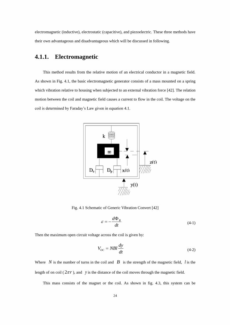
4.1.1. Electromagnetic
This method results from the relative motion of an electrical conductor in a magnetic field.
As shown in Fig. 4.1, the basic electromagnetic generator consists of a mass mounted on a spring
which vibration relative to housing when subjected to an external vibration force [42]. The relation
motion between the coil and magnetic field causes a current to flow in the coil. The voltage on the
coil is determined by Faraday’s Law given in equation 4.1.
Fig. 4.1 Schematic of Generic Vibration Convert [42]
Bd
dt
(4-1)
Then the maximum open circuit voltage across the coil is given by:
OC
dyV NBl
dt (4-2)
Where N is the number of turns in the coil and B is the strength of the magnetic field, l is the
length of on coil ( 2 r ), and y is the distance of the coil moves through the magnetic field.
This mass consists of the magnet or the coil. As shown in fig. 4.3, this system can be

25
reasonably described by a second-order mass ( m )-spring ( k ) –damper ( pD ) system. The
equation of motion of the mass relative to the housing when driven by a sinusoidal vibration force
F is given by [43]:
2
2sinp o em
d x dxm D kx F t F
dt dt (4-3)
where F is the movement between mass and housing (or between magnet and coil). pD is the
parasitic damping force due to air resistance and material loss, emF is the electromagnetic force
due to the force between the current in the coil and magnet. /n k m is a mechanical
resonant frequency. So it is important to have the frequency of the driving force equal to the
mechanical resonant frequency to maximize displacement. When em pD D , the output power
will reach the maximal electrical power, the average generated electrical power can be obtained
from [42]:
2 2
20
1( )
2( )
TO
avg em em
p em
FdxP D dt D
T dt D D
(4-4)
In order to harvest the maximal power, there are two aspects should be taken into account: for one
thing, a strong magnet has to be attach to the generator. For another hand, how much this magnet
and its motion would affect electronics is another challenge.
4.1.2. Electrostatic
The basic of electrostatic energy conversion is a variable capacitor [11]. Electrostatic
generators are mechanical devices that produce electricity by using manual power [44][45],
which consists of two conductors separated by a dielectric such as capacitor. As the conductor
moves, the energy stored in the capacitor changes, that providing the mechanism for mechanical
to electrical energy conversion. An electrostatic generator is always illustrated by a simple
rectangular parallel plate capacitor. There are three types of electrostatic generator [11]: in-phase
overlap convert, in-phase gap closing convert and out-of-plane gap closing convert.
The voltage generated by the generator is expressed by equation (4-5) [12]:

26
0
Q QdV
C lw (4-5)
where Q
is the charge of capacitor, d is the distance between two plates, l is the length of the
plates, w is the width of the plate, and 0 is the dielectric constant of free space. The voltage can
be increased by decrease the capacitance [46]. Then the energy converted by generator can be
expressed by (4-6):
221 1
2 2 2
QE QV CV
C (4-6)
4.1.3. Piezoelectric
Piezoelectric materials are materials that convert mechanical energy from vibrations, force
and pressure into electricity. At present, polycrystalline ceramic is the most common piezoelectric
material. Typically, the constitutive equations for a piezoelectric material are given by following
equation [12]:
dEV
(4-7)
D E d (4-8)
where is mechanical strain, is the mechanical stress, Y is the modules of elasticity (Young’s
Modules), d is the piezoelectric strain coefficient, E is the electric field, D is the electrical
displacement (charge density), is the dielectric constant of the piezoelectric material. The open
circuit which means that the electrical displacement ( D ) is zero is defined as:
OC
dtV
(4-9)
where t
is thickness of the piezoelectric material.
4.1.4. Comparison of Conversion Methods
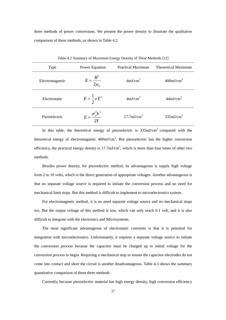
It is important to discuss both of the qualitative and quantitative comparison of the above
27
three methods of power conversions. We present the power density to illustrate the qualitative
comparison of these methods, as shown in Table 4.2.
Table 4.2 Summary of Maximum Energy Density of Three Methods [12]
Type Power Equation Practical Maximum Theoretical Maximum
Electromagnetic
2
02
BE
4mJ/cm
3 400mJ/cm
3
Electrostatic 21
2E E 4mJ/cm
3 44mJ/cm
3
Piezoelectric
2 2
2
y kE
Y
17.7mJ/cm3
335mJ/cm3
In this table, the theoretical energy of piezoelectric is 335mJ/cm3
compared with the
theoretical energy of electromagnetic 400mJ/cm3. But piezoelectric has the higher conversion
efficiency, the practical energy density is 17.7mJ/cm3, which is more than four times of other two
methods.
Besides power density, for piezoelectric method, its advantageous is supply high voltage
from 2 to 10 volts, which is the direct generation of appropriate voltages. Another advantageous is
that no separate voltage source is required to initiate the conversion process and no need for
mechanical limit stops. But this method is difficult to implement to microelectronics system.
For electromagnetic method, it is no need separate voltage source and no mechanical stops
too. But the output voltage of this method is low, which can only reach 0.1 volt, and it is also
difficult to integrate with the electronics and Microsystems.
The most significant advantageous of electrostatic converter is that it is potential for
integration with microelectronics. Unfortunately, it requires a separate voltage source to initiate
the conversion process because the capacitor must be charged up to initial voltage for the
conversion process to begin. Requiring a mechanical stop to ensure the capacitor electrodes do not
come into contact and short the circuit is another disadvantageous. Table 4.3 shows the summary
quantitative comparison of these three methods.
Currently, because piezoelectric material has high energy density, high conversion efficiency

28
and other excellent advantageous, this method has been widely used in ambient energy harvesting.
So we would discuss this method detail in following.
Table 4.3 Summary Quantitative Comparison of Three Methods [12]
Type Advantageous Disadvantageous
Electromagnetic No separate voltage source and no
mechanical stops.
Low output voltage (0.1 volts);
Hard to integrate to micro
electric system.
Electrostatic Easy to integrate to micro electric
system.
Need separate voltage source
to start and mechanical stops
to prevent from short circuit.
Piezoelectric
High output voltage (2-10volts);
No separate voltage source and no
mechanical stops.
Generator size is too big to
integrate to micro electric
systems.
4.2. Piezoelectric Model
Fig. 4.2 is the mechanical model of piezoelectric. The piezoelectric beam shakes vertically,
and conversion the mechanical energy to AC current. Thus the electromechanical energy
conversion mechanism of the beam can be modeled with a current source in parallel with a
capacitor, this current source also can be replaced by a voltage source series with a capacitor, as
shown in Fig. 4.3 and Fig. 4.4.[47][48][49]. In Fig. 4.4, the ( )thV t can be calculated by:
1( ) ( )th P
P
V t i t dtC
(4-10)

29
Piezoelectric Beam
U(t)=umcos(ωt )
Fig. 4.2 Mechanical Model of Piezoelectric
AC
ip(t)
i(t)
ic(t)
Lo
ad
Cp
Vp(t)
Fig. 4.3 Piezoelectric Model as Current Source
AC
Vth(t)
Lo
ad
Cp
Vp(t)
Fig. 4.4 Piezoelectric Model as Voltage Source
In order to rectify the AC current to DC current, typically, a full-bridge diode rectifier is used
to connect to generator, as shown in Fig. 4.5. FC is a filter capacitor which connect to the load. In
this case, the maximum rectified voltage occurs when 0loadR . This is also called open circuit
voltage, this value is [48]:

30
2
POC
P
IV
C (4-11)
AC
ip(t) ic(t)
Cp
Vp(t)
+
_
CF
VF
+
_
Lo
ad
Fig. 4.5 Piezoelectric Model with Full-Bridge Rectifier
Where is the frequency of vibration. When it connects to load, the piezoelectric maximum
voltage is limited by filter voltage: ( )p Fv t V , and if filter voltage is half of open circuit voltage:
2
ocF
VV (4-12)
The output power will reach the maximum power, this maximum average power is [49]:
2
max2
p OCC VP
(4-13)

31
5. Other Energy Source
Besides mentioned energy source above, other energy sources are available to supply power
to microelectric system, such as human power, wind (air flow) and electromagnetic field [10][50].
5.1. Human Power
Human power is passive power source in that the human does not need to do anything other
than that what they would normally do to generate power. The average human body burns about
10.5MJ of energy per day [10]. There are some projects has proposed tapping into some of this
energy to power wearable electronics such as watches. [51]. MIT has developed a piezoelectric
shoe that produces an average of 330μW/cm2 while a person is walking [51].
5.2. Wind/Air Flow
Wind power has been used as a large scale power source for a long time, it is common today
still. This paper focuses on the small scale of wind power. The power from moving air can be
calculated as follow [10]:
31
2P Av (5-1)
Where is the density of air, this is approximately 1.22kg/m3
normally, A is the cross sectional
area and v is the air velocity.
In large scale wind system, the maximum efficiency is about 40% which depends on the air
velocity and average efficiency is 20% normally. A low air velocity leads to the efficiency low
than 20%. Fig. 5.1 shows the power density from air flow [10], the output power is about
0.2mW/cm2 if the efficiency is 5% when air velocity is 5m/s. It is reasonable that convert the air
flow to electrical power at small scale.

32
Fig. 5.1 Power Density from Air Flow
5.3. Electromagnetic
Recently, ambient electromagnetic especially RF energy is a possible energy source for
energy harvesting. RF energy means available through public telecommunication service such as
GSM and WLAN frequencies [50]. But this energy is limited by the power density and need large
area to collect usable energy, the ideal collected power can be expressed as:
24
et
AP P
r (5-2)
Where tP is the transmission power from source,
eA is the receive area, r is the distance. When
harvesting in the GSM or WLAN band, the distance ranging from 25m to 100m from a GSM base
station, power density ranging from 0.1 to 1.0 mW/m2 which is expected by single frequencies.
[51]. Alternatively, a total antenna surface can be minimized if one uses a dedicated RF source,
which can be positioned close to the sensor node, thereby limiting the transmission power to levels
accepted by international regulations [50].
Powercast Company has developed a universal chip for the purpose of replace the battery
charger. The frequency is 906MHz and the power is 2-3W, and 15mW of power is received at
30cm distance.

33
6. Energy Storage
There are two choices available for energy storage: super capacitor and batteries. Generally
speaking, batteries are mature technology. Super capacitors have higher power density and high
life time than batteries. It has been used to handle short duration power surges [54].
6.1. Super Capacitor
Compared with batteries, super capacitors have virtually infinite recharge cycles and are ideal
for frequent pulsing applications. Unfortunately, super capacitors have higher leakage current,
large size and cost [53]. Super capacitor can be modeled as a power source:
1 max( ) max( ( ( ) ( ) ( )) , )in out leakt
E t P t P t P t dt E (6-1)
Where inP is the power from environmental energy sources,
outP is output power and leakP
is the leakage power caused by leakage current. The totally energy in capacitor is expressed by:
21
2E CV (6-2)
Where C is the capacitance of capacitor, V is capacitor voltage. For example, if two
capacitors with 22F and 50F, there storage energy are 68.75J and 156.25J respectively. The
leakage current of super capacitor increases with the decreases of their capacitance and the rated
voltage decreases with the increases of their capacitance, a capacitor with 22F has 0.049mA
leakage current and 2.5V rated voltage, a capacitor with 50F has 0.073mA leakage current and
2.3V rated voltage. Fig. 6.1 shows the super capacitor leakage in 24 hours.
Configuration of super capacitor also plays an important role in choosing a suitable super
capacitor in a system [55]. It means series or parallel with two or more super capacitors. For one
hand, series lower the leakage current, but it results half the total capacitance. For another hand,
parallel two super capacitors can increase the capacitance and increase the leakage current.

34
Fig. 6.1 Super Capacitor Leakage Diagram
6.2. Batteries
Batteries are used in the condition that when the energy in super capacitor is exhausted. It
needs to hold energy for a long period of time and low leakage current [55]. There are three types
of rechargeable batteries are commonly used at present: Nickel Cadmium (NiCd), Nickel Metal
Hydride (NiMH) and Lithium based (Li+). Lithium rechargeable battery has the lowest leakage
current, highest density, high recharge cycle and high voltage for one cell. But it needs a complex
charging circuit to protect battery. The NiCd battery is less used because of its low energy density.
The NiMH battery has memory effect and limited by the leakage current.
35
7. Adaptive-Topology MPPT Method
As discussed in above chapters, solar cell is able to scavenge more energy than other energy
source. Here we present a novel maximum power point tracking method on solar cells: adaptive
topology MPPT method, this method also can be implemented in other energy source such as
vibration and thermal.
7.1. Solar Cell Output Characteristics
The core of maximum power point tracking is impedance matching. The output impedance of
solar cell is affected by many factors such as environment temperature and irradiance. It is not a
constant value and varies from time to time. The solar cell array with different connection
methods also occur the change of output impedance, it requires different resistors to connect to the
output of solar cell to match the output impedance.
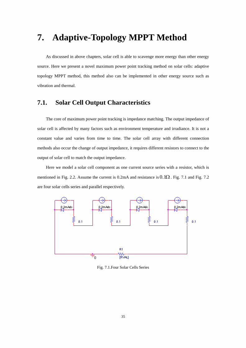
Here we model a solar cell component as one current source series with a resistor, which is
mentioned in Fig. 2.2. Assume the current is 0.2mA and resistance is 0.1 . Fig. 7.1 and Fig. 7.2
are four solar cells series and parallel respectively.
Fig. 7.1.Four Solar Cells Series
36
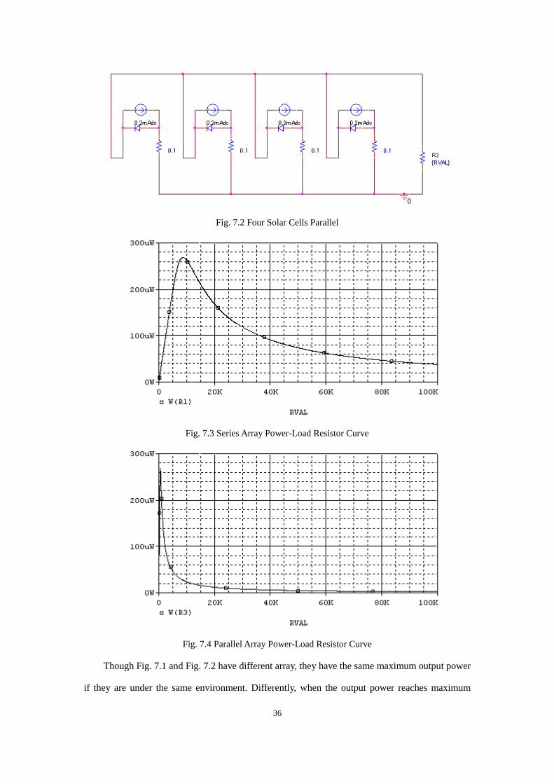
Fig. 7.2 Four Solar Cells Parallel
Fig. 7.3 Series Array Power-Load Resistor Curve
Fig. 7.4 Parallel Array Power-Load Resistor Curve
Though Fig. 7.1 and Fig. 7.2 have different array, they have the same maximum output power
if they are under the same environment. Differently, when the output power reaches maximum

37
output power, the loads is different. The matching load is about 8KΩ while all cells are series as
shown in Fig.7.3 and the matching load is about 1KΩ while all cells are parallel which is
described in Fig, 7.4.
7.2. MPPT Method and Model
According to above analysis, we present a novel MPPT method: for one thing, we change the solar
cell array as series, parallel or series-parallel mixed array. Under the same environment, these arrays
has the same maximum output power theoretically but requiring different load to match the impedance.
For another thing, there are many load resistors with different resistances could be choice to connect to
the solar cell array in order to choose a load to maximize the output power.
If four solar cells are used in this system, as shown if Fig. 7.5 there are three arrays are able to
choose. Similarly, 2n
solar cells could convert to 1n arrays.
Solar Cell Solar Cell Solar Cell Solar Cell
Solar Cell
Solar Cell
Solar Cell
Solar Cell
Solar Cell
Solar Cell
Array 1
Array 2
Array 3
Solar Cell
Solar Cell
Fig. 7.5 Available Arrays of Four Solar Cells
For the purpose of conversion the solar cells array automatically, a solar cells variation
diagram has been designed, as shown in Fig. 7.6. In this diagram, the cathode of Solar cell P1
connects to ground. If switch S1, S2 and S3 are on, S4-S9 are off, the array convert to array 1 as
shown in Fig.7.7, all solar cells are series in this case, which is like array 1 as shown in Fig. 7.5;
when S1-S3 are off, and S4-S9 are on, as shown in Fig. 7.7, Array 2, all solar cells are parallel,
this is described as array 2 in Fig.7.5; if S1, S3, and S5,S6 are off, S4,S5, S8, S9 and S3 are on, the
solar cells array is like array 3 shown in Fig. 7.7. This array is equal to Array 3 in Fig. 7.5. These

38
three types of array have the same output maximum power but required different matching loads.
P1
P2
P3
P4
S5S4 S1
S2
S3
S7S6
S9S8
Fig. 7.6 Solar Cell Control Diagram
P1
P2
P3
P4
P1
P2
P3
P4
P1
P2
P3
P4
Array 1 Array 2 Array 3
Fig.7.7 Conversion of Solar Cell Array
In order to match the impedance of solar cells array, there are many resistors with difference
resistance and switches can be connected to the solar cell array, as shown in Fig. 7.8. The entire
resistance can be calculated by:
1 2
1
1 1 1...
n
R
R R R
(7-1)
All switches are controlled by a MCU, the total resistance rang from the minimum resistance to
the maximum resistance. The number of available resistance is determined by the number of
resistors. For example, if there are n resistors, the available resistance is 2n, and if available
solar cells array is m , there are 2nm combination modes.

39
…
R1
R2
Rn-1
Rn
Fig. 7.8 Resistor Connection Diagram
7.3. System and Control Flow
Our system architecture is presented in Fig. 7.9, it consists five parts: solar cells, matching
resistors, DC/DC, super capacitor and MCU. Solar cells and matching resistors are controlled by
the MCU to output the maximum power as possible. Then the DC/DC converts the output voltage
of matching resistor to working voltage such as 3.3V, 2.5V or 1.7V. The super capacitor reserves
the power to supply to MCU. Fig. 7.12 is the block diagram with m solar cells and n matching
resistors.
Solar Cells Matching Resistor DC/DC
MCU SuperCapacitor
Fig. 7.9 Energy Harvesting System Architecture
Assuming there are m available solar cell arrays in solar cells block and n available resistors
in matching resistor block, so there are m n possible combination modes in this system. Fig.
7.10 is the flow chart of MCU in energy harvesting system. In this chart, Solar(i) means the i th
solar cells array and Resis(j) is the j th matching resistor. At the beginning, it iterates all possible
combination modes of solar cells and matching resistors and measure the output voltage of solar
cells array, store it in the memory of MCU. Then according to equation (2-8) to calculate the
constant k , compare the constant k with refk , refk is a reference k which is raging from 0.60 to

40
0.70 in this paper. The array corresponding to k which is closest to refk is the maximum power
point array (MPP array). The environment such as irradiance and temperature changes frequently,
so the system works under this array for a period and start to search a new MPP array.
Start
Solar(i)<m+1
Resis(j)<N+1
Measurement of V(ij),j++
j=1,i++
P(ij)=|(V(ij)/Vref)-kref|
Yes
Yes
No
Pmin=min(P(ij)),I=I,J=j
Solar(I),Resis(J)
Delay
i=1,j=1
No
Fig 7.10 Flow Chart of flow chart of MCU in Energy Harvesting System

41
8. Experimental Result
In this chapter, we have measured thermal generator, vibration piezoelectric generator and
variable array solar cells and compare these experimental results.
8.1. Thermal Generator Result
ECT 310 Perpetuum Module is a thermoelectric generator module developed by EnOcean
[56], which is used in this paper. This module includes a DC/DC convertor, which enable to use
heat as their power source. Typically, this module connects an external low cost peltier element
TEC2L-15-15-5.6/73. Fig. 8.1 and Fig. 8.2 is a picture of this module and element. The size of this
module and component is 14.0×14.0×5.0mm and 15.0×15.0×4.0mm respectively.
Fig. 8.1 ECT-310 DC/DC Convertor

42
Fig. 8.2 ECT-310 Element
As shown in Table. 8.1 [57], the start-up input voltage of ECT is 20mV, and maximal input
voltage is 500mV. Fig. 8.3 is the Vin-Vout Characteristics of ECT-310, the input voltage is
unloaded input voltage.
Table. 8.1 Technical Data of ECT 310 [57]
Peltier Element Characterizes
Type TEC2L-15-15-5.6/73CS
Temperature coefficient 12.5Mv/K
Internal resistance 1.44Ω
Thermal conductivity 0.046 W/K
ECT 310 DC/DC Convertor
Typical Value
Vin input voltage start-up 20 mV
Vin input voltage max. 500mv
Vout output voltage @ Vin=20…50 mV 3…4V
Vout output voltage @ Vin=20…500mV 3…5V(Rload<10MΩ)

43
Fig. 8.3 Vin-Vout Characteristics of ECT-310
The open circuit output voltage (VOC) of peltier element is proportion to the temperature
gradient between two sides of peltier element TEC2L-15-15-5.6/73. As shown in Fig. 8.4, it exists
a linear relationship between open circuit output voltage and temperature gradient in two sides of
peltier elements. This open circuit voltage is the maximal output voltage of element, as mentioned
above, the maximal power point voltage is half of open circuit voltage. This voltage could reach
several mW typically, which need connect a boost DC/DC to boost the voltage to a typical
reference voltage such 3.3V etc. This is the reason why we use a boost DC/DC here.
Fig. 8.4 Vout as a function of temperature gradient

44
Fig. 8.5 and Fig. 8.6 show the output characteristics of the element used in this experiment,
which has the same result as described in Fig. 3.3 and Fig. 3.4. A variable resistance was used as a
load and measured in three temperature gradients: 10℃, 18℃ and 33℃. The output current (Iout)
linearly decreased with the output voltage in the same temperature gradient and the output voltage
and current increase with the raise of temperature gradient. As shown in Fig. 8.6, the maximal
output power is nearly the half of the maximal output voltage, this maximal output voltage is
equal to the open circuit output mentioned above, which verified the theoretical formula (3-8).
Fig. 8.5 Experimental Thermoelectric Generator Output Current-Voltage Curve
Fig. 8.6 Experimental Thermoelectric Generator Output Power-Voltage Curve

45
Fig 8.7 shows the output power of thermoelectric element and DC/DC convertor. The blue
star is the output power of TEC2L-15-15-5.6/73CS Peltier element. This output power increased
by the growing of temperature gradient. When the temperature gradient is 5℃, the output power is
about 0.1mW, at 10℃ temperature gradient, this power is 0.45mW. By the temperature gradient
reaching to 15℃, this power will reach to 1mW. Meanwhile, if the element connects to ECT 310
DC/DC convertor directly, the transfer efficiency can be calculated by:
max _ _ _
max _ / _ _
imal element output power
imal DC DC output power
P
P (8-1)
Fig, 8.7 Output Power of Thermoelectric Element and DC/DC Convertor
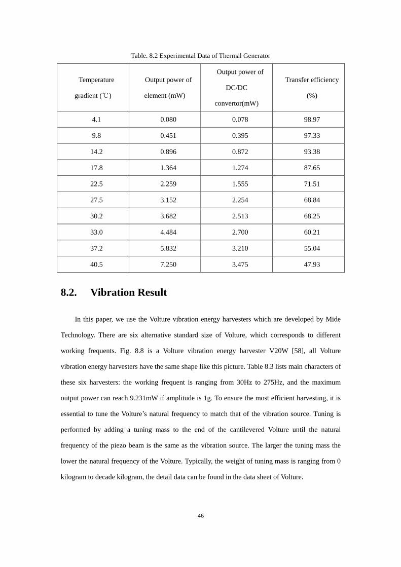
This efficiency is more than 95% when temperature gradient is less than 15℃.Table 8.2 is the
experimental data. It is clear that the transfer efficiency decrease with the increase of temperature
gradient. Though the transfer efficiency decline, the output power of DC/DC convertor raise
smoothly compared with the increase of output power of element.
46
Table. 8.2 Experimental Data of Thermal Generator
Temperature
gradient (℃)
Output power of
element (mW)
Output power of
DC/DC
convertor(mW)
Transfer efficiency
(%)
4.1 0.080 0.078 98.97
9.8 0.451 0.395 97.33
14.2 0.896 0.872 93.38
17.8 1.364 1.274 87.65
22.5 2.259 1.555 71.51
27.5 3.152 2.254 68.84
30.2 3.682 2.513 68.25
33.0 4.484 2.700 60.21
37.2 5.832 3.210 55.04
40.5 7.250 3.475 47.93
8.2. Vibration Result
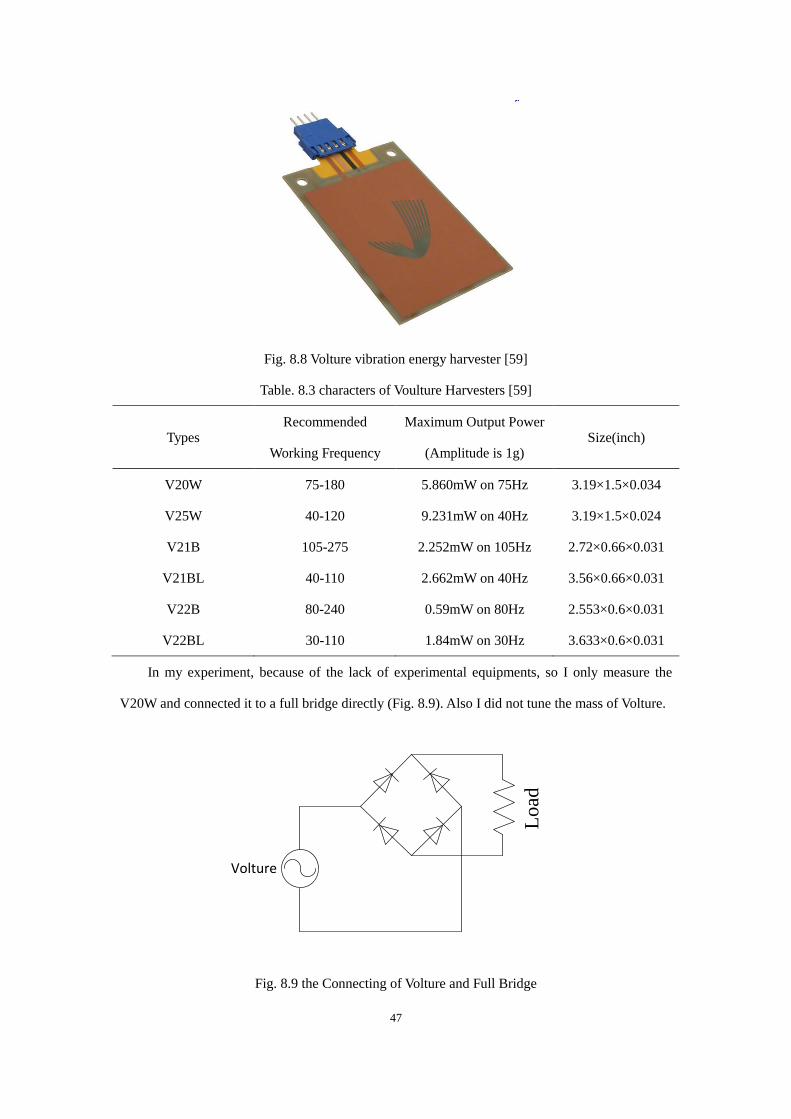
In this paper, we use the Volture vibration energy harvesters which are developed by Mide
Technology. There are six alternative standard size of Volture, which corresponds to different
working frequents. Fig. 8.8 is a Volture vibration energy harvester V20W [58], all Volture
vibration energy harvesters have the same shape like this picture. Table 8.3 lists main characters of
these six harvesters: the working frequent is ranging from 30Hz to 275Hz, and the maximum
output power can reach 9.231mW if amplitude is 1g. To ensure the most efficient harvesting, it is
essential to tune the Volture’s natural frequency to match that of the vibration source. Tuning is
performed by adding a tuning mass to the end of the cantilevered Volture until the natural
frequency of the piezo beam is the same as the vibration source. The larger the tuning mass the
lower the natural frequency of the Volture. Typically, the weight of tuning mass is ranging from 0
kilogram to decade kilogram, the detail data can be found in the data sheet of Volture.
47
Fig. 8.8 Volture vibration energy harvester [59]
Table. 8.3 characters of Voulture Harvesters [59]
Types Recommended
Working Frequency
Maximum Output Power
(Amplitude is 1g) Size(inch)
V20W 75-180 5.860mW on 75Hz 3.19×1.5×0.034
V25W 40-120 9.231mW on 40Hz 3.19×1.5×0.024
V21B 105-275 2.252mW on 105Hz 2.72×0.66×0.031
V21BL 40-110 2.662mW on 40Hz 3.56×0.66×0.031
V22B 80-240 0.59mW on 80Hz 2.553×0.6×0.031
V22BL 30-110 1.84mW on 30Hz 3.633×0.6×0.031
In my experiment, because of the lack of experimental equipments, so I only measure the
V20W and connected it to a full bridge directly (Fig. 8.9). Also I did not tune the mass of Volture.
Volture
Load
Fig. 8.9 the Connecting of Volture and Full Bridge

48
The out power frequency is 100Hz, there are three amplitudes: 3g, 4.5g and 6.5g. It is clear
that the maximum output power is 0.12mW, 0.3mW and 0.66mW when amplitudes are 3g, 4.5g
and 6.5g respective and the output power is proportion to the square of the amplitude.
Fig. 8.10 the Output Power of V20W without Tuning
8.3. Solar Cells Array Result
In this experiment, we have developed a solar cell array including 4 solar cells, the open
voltage of one solar cell is from 2.8V to 3.2V, the size is 3.5cm×1.4cm for one solar cell. Thus
there are three available solar cell arrays as mentioned in Fig. 7.5: four series (4-S), four parallel
(4-P) and two parallel with two series (P-S).
As mentioned in chapter 2, the characteristic of solar cells is presented by voltage-current
curve. In this experiment, first we have measured the solar cell array under low, medium and high
irradiance with three different arrays: 4-S, 4-P, and S-P. These solar cells are connected with wire
directly. There is no other component such as transistor or resistor to consume any energy. The
voltage-current curve is shown from Fig. 8.11 to Fig. 8.13 under low, medium and high irradiance
conditions. It is clear from this diagram that the 4-S has the highest open voltage and lowest short
current, 4-P has the lowest open voltage and highest short current and S-P is in between. Fig. 8.14
to Fig. 8.16 is their voltage-power curve respectively. Their maximum power is 2.57mW, 4.25mW
and 7.73mW under low, medium and high irradiance conditions respectively.

49
Fig. 8.11 the Voltage-Current curve of Solar Cell Array under low irradiance condition
Fig. 8.12 the Voltage-Current curve of Solar Cell Array under medium irradiance condition
Fig. 8.13 the Voltage-Current curve of Solar Cell Array under high irradiance condition

50
Fig. 8.14 the Voltage-Power curve of Solar Cell Array under low irradiance condition
Fig. 8.15 the Voltage-Power curve of Solar Cell Array under medium irradiance condition
Fig. 8.16 the Voltage-Power curve of Solar Cell Array under high irradiance condition

51
The above mentioned data are ideal maximum power point. In practice, according to Fig. 7.9,
the novel MPPT method should connect several transistors and resistors into circuits. These
components have leakage current and consume power which reduce the collected power and
change the voltage-current characteristics. The following figures from Fig. 8.17 to Fig. 8.19 are
voltage-current curve with MPPT circuit under low, medium and high irradiance conditions. Fig.
8.20 to Fig. 8.22 is respective voltage- power curve. Their maximum power is 1.88mW, 3.88mW
and 6.50mW under low, medium and high irradiance conditions respectively. As shown in Table.
8.4, the MPPT efficiency is 73.15%, 91.29% and 84.09% respectively under low, medium and
high irradiance.
Table 8.4 Comparison of Solar Cells Array Efficiency
Low Irradiance Medium Irradiance High Irradiance
Ideal Power (mW)①
2.57 4.25 7.73
Practical Power (mW)②
1.88 3.88 6.50
Efficiency 73.15% 91.29% 84.09%
① The solar cells connect with wire directly.
② MPPT circuit with electrical components.
Fig. 8.17 the Voltage-Current curve of Solar Cell Array under low irradiance condition

52
Fig. 8.18 the Voltage-Current curve of Solar Cell Array under medium irradiance condition
Fig. 8.19 the Voltage-Current curve of Solar Cell Array under high irradiance condition
Fig. 8.20 the Voltage-Power curve of Solar Cell Array under low irradiance condition

53
Fig. 8.21 the Voltage-Power curve of Solar Cell Array under medium irradiance condition
Fig, 8.22 the Voltage-Power curve of Solar Cell Array under high irradiance condition
In this experiment, we choose four resistors as the load matching resistors, as shown in Fig.
8.23. There are four resistance values can be chosen to match the output of solar cells array. The
maximum load resistance is max[( 1 4), 2, 3)]R R R R , and the minimum load resistance is less
than min[( 1 4), 2, 3]R R R R , as shown in Table. 8.4, this is available load resistance. Here we
choose four resistances: 1 58 , 2 31 , 3 14.2 , 4 17R k R k R k R k , then the actual
load resistance are: 75Ω, 12Ω, 22Ω and 8.6Ω respectively. The maximum output voltage of solar
cells array can reach about 12V in this experiment and the sample range of ADC is from 0-2.5V in
MCU, so we series a resistor with R1, the actual output voltage of solar cell array outV which is
used in chapter 7.3 can be expressed by:

54
1 44
4
R ROUT R
R
V VV V
V
(8-2)
R1
R2
R3
S1
S2
R4
Fig. 8.23 Load Matching Resistors
Table 8.4 Load Resistance Values
Load Resistance Status of S1 Status of S2
1 4R R Off Off
( 1 4) 2
( 1 4) 2
R R R
R R R
On Off
( 1 4) 3
( 1 4) 3
R R R
R R R
Off On
( 1 4) 2 3
( 1 4) 2 3
R R R R
R R R R
On On
As mentioned above, there are 3 solar cells arrays and 4 resistances can be choose to
optimize the output of solar cells, so there are 12 connections. When we connect a MCU to solar
cells array, the system starts to switch all available choices, then according to FOSV method, the
system can calculate the maximum output voltage and switch to corresponding solar cell array and
resistor itself. Table 8.5 shows the voltage and current we measured in different connection. We
have set the switching time is 1.6s. At beginning of start, there is a about 1,100ms start time to
start switching. Between the switching of two solar cells array, it exists approximate 33ms of
switching delay as shown in Fig. 8.24, which is caused by the charging of transistor capacitor.

55
Table 8.5 the Voltage-Current of Switching
Connections Voltage
(Volt)
Current
(mA)
Power
(mW)
All Series
Resistance 1 6.33 0.50 3.165
Resistance 2 10.49 0.11 1.154
Resistance 3 8.71 0.35 3.049
Resistance 4 6.37 0.49 3.121
All
parallel
Resistance 1 2.75 0.41 1.128
Resistance 2 2.95 0.02 0.059
Resistance 3 2.91 0.10 0.290
Resistance 4 2.85 0.21 0.599
Two
Series
with two
parallel
Resistance 1 4.82 0.51 2.458
Resistance 2 5.75 0.05 0.287
Resistance 3 5.41 0.21 1.136
Resistance 4 5.06 0.38 1.923
Fig. 8.24 Switching Delay
Table 8.6 lists the ideal maximum power under different irradiances and the maximum output
power using this MPPT method. The ideal output maximum power in the shadow in outdoor
ranges from 3mW to 6mW, and it is more than 6mW which under direct sun in outdoor. If we put

56
the solar cells array next to the window indoor or in the dusk, the maximum power is less than
3mW. As shown in Table. 8.6, this MPPT efficiency can reach 60% to more than 82.4% in outdoor
in daytime. But the efficiency is less than 40% in door or in the dusk.
Table 8.6 Power Comparison of Solar Cells Array
Ideal Maximum
Power (mW) 2.06 2.75 3.56 4.47 4.68 5.05 5.88 9.78 10.29
Actual power
(mW) 0.41 0.88 2.11 3.44 3.48 4.16 4.94 6.87 7.81
MPPT Efficiency 20.1% 32% 59.2% 77.1% 74.3% 82.4% 84.0% 70.3% 76.0%
Since the capacitor is seen as a short to the solar cell when the connect together, the
traditional voltage regulator such as PWM DC-DC converter and linear regulator would not
function properly because solarV would fall to
capV and deviate from mppV , a PFM regulator
is designed in literature [60] to resolve this problem.
In this thesis, we connected a super capacitor with the capacitance of 22F to the DC/DC, as
shown in Fig. 8.25, this is the DC/DC circuit diagram, the capacitor rating voltage is 2.5V. The
DC/DC output voltage is 2.8V, this is larger than the rating voltage of capacitor, so it fulfills the
charging requirement. Here we compared four different solar cells array connection: MPPT
method, all series without MPPT (All Series Mode), all parallel without MPPT (All Parallel
Mode), and two parallel with two series without MPPT (Series-Parallel Mode). The experimental
result shows in Table. 8.7. The voltage is 2.3V which is able to drive the MCU and wireless sensor
nodes. It is clear that this MPPT method has higher current than all series mode and all parallel
modes, but it performs not good compared with series-parallel mode sometimes.
Vin
Cap
Vin2
EN
STBY
SW
Vout
GND
Vin
2.2μF
4.7μF
1μF
47μF
100μH
22FSuperCapacitor
Fig. 8.25 DC/DC Circuit

57
Table 8.7 Charging Current and efficiency of Different Solar Cells Array Connection
Maximum
Power(mW) 4.39 5.21 6.89 7.51 10.02
MPPT 0.812 0.897 1.114 1.360 1.857
All Series 0.622 0.542 0.505 0.982 1.829
All Parallel 0.064 0.259 0.595 0.337 0.440
Series-Parallel 1.204 0.862 1.028 1.641 2.609
Charging efficiency
MPPT 42.4% 39.6% 37.1% 41.7% 42.6%
All series 32.5% 23.9% 16.8% 30.1% 42.0%
All parallel 3.3% 11.4% 19.8% 10.3% 10.1%
Series-Parallel 63.0% 38.0% 34.2% 50.0% 60.0%
8.4. Power Supply to MCU
In order to drive a wireless sensor node, here we assume our sensor node has three modes:
sleep mode, start mode and active mode. The active mode is that the sensor node transmits data to
other nodes, it consumes 25mA current, the start mode is that the node prepares to send data, it
consumes 5mA current, and sleep mode as the name means the node do nothing which only
consumes 2μA.
We use MSP430-5379 as our MCU, this is a low power microcontroller; it only consumes
6μA in sleep mode. The average consuming current of MCU can be calculated by equation 8-3,
switching switching MCUsleep MCUsleep
MCU
switching MCUsleep
t i t ii
t t
(8-3)
For example, assume the switching time switchingt is 10s, and MCU track the maximum power
point every 10 minutes, then sleep time MCUsleept is 600s. The sleep current is ideal 6μA, the
switching current switcht is 558μA as we measured, then the average MCU current
MCUi is
15.05μA.

58
25mA
5mA
2μASleep
Start
active
time
current
Fig. 8.26 Power Consumption of Wireless Sensor Node
According to the following equation:
arg
1( ( 0.002) )active active start start sleep ch ing MCUn t i t i i i i
n
(8-4)
Where n is the maximum working frequency in one second of sensor node. We are able to
calculate the minimum duration time of sensor node with different charging current, as shown in
Table 8.7.
Table.8.7 Duty Cycle Compared with Different Charging Current
Charging Current(μA) 100 300 500 800 1000 1500 2000
Duration Time(ms) 362 106 62.1 38.3 30.5 20.2 15.1

59
9. Conclusion and Future Work
In this thesis, my thesis focuses on the following tasks:
1. We have studied the most matured ambient energy source: vibration, thermal and solar; and
other potential energy source such as human power, wind and air flow, electromagnetic by
literature review.
2. Setup basic analytical models for these ambient energy sources, and list available and exiting
MPPT methods.
3. Present a novel MPPT method of solar cells, build the mathematic model and design the
analog circuits of it; besides solar, this MPPT method also is available to help thermal and
vibration to track the MPP.
4. According to mathematical models of vibration, thermal and solar, we have measured the
output power data and verify their characteristic. Also, we give the efficiency of this novel
MPPT method, the experimental result shows that its efficiency is 60%-80% in micro system.
5. Calculate the theoretical working time of sensor node by using this MPPT method.
This novel MPPT method has high energy conversion efficiency which reach 60%-80%
commonly in micro system while connect to load directly; A small size of 1.4cm×14cm for four
solar cells is able to drive the sensor nodes for a duration time of decades micro seconds which
depends on irradiance.
In the future, there are also following aspects should take into account to improve this work:
For one thing, in order to optimize the output efficiency, it is better to product PCB board and
chooses low power consumption components; this will decrease the leakage current. Besides, it
also need optimize MUC to decrease the power consumption.
For another thing, it is necessary to verify this novel MMPT method on vibration and thermal
sources. It should measure and calculate the experimental conversion efficiency.
At last, PFM regulator or charging circuit should implement in this design to charge a
supercapacitor or battery.

60
References
[1] P.LI, Y. Wen, Young, P. Liu, X. Li ,and C. Jia, “A Magnetoelectric Energy Harvester and
Management Circuit for Wireless Sensor Network,” Sensors and Actuators A: Physical,
157(2010) 100-106.
[2] J. R. Farmer, “A Comparison of Power Harvesting Techniques and Related Energy Storage
Issues,” M.S Thesis, Dept. Mech. Eng., Virginia Polytechnic Institute and State Univ.
Blacksburg, VA, 2007.
[3] F. Blatt, P. Schroeder, C. Foiles and D. Greig, “Thermoelectric Power of Materials,” New
York: Plenum press, 1976.
[4] G. Nolas, J. Sharp, H. Goldsmid, “Thermoelectrics: Basic Principles and New Materials
Devwlopments,” New York, Springer, 2001.
[5] O. Mah, “Fundamental of Photovoltaic Materials,” National Solar Power Research Institute,
Inc., 1998.
[6] J.Damaschke, “Design of a Low-Input-Voltage Converter for Thermoelectric Generator,”
IEEE Transaction on Industry Application 1997, 33(5):1203-7.
[7] R. Myers, “The Basic of Physics,” Westport, Conn, Greenwood Press, 2006.
[8] R. Elliot, “Electromagnetics: History, Theory, and Application,” Piscataway: IEEE PRESS,
1993.
[9] A. Harb, “Energy Harvesting: State-of-the-art,” Renewable Energy, vol. 36, pp.2641-2654,
2011.
[10] S. Roundy, D. Steingart, L. Frechette, P. Wright and J. Rabaey, “Power Source for Wireless
Sensor Network”, Computer Science Vol. 2920/2004, pp.1-17.
[11] S. Roundy, P. K. Wright, and J. Rabaey,, “A Study of Low Level Vibrations as a Power
Source for Wireless Sensor Nodes,” Computer Communication 26 (2003) 1131-1144.
[12] S. Roundy, P. K. Wright, and J. M. Rabaey, Energy Scavenging for Wireless Sensor Network
with Special Focus on Vibration. Kluwer Academic Publishers, 2004, pp. 49.
[13] V. Jovanvic, S. Ghamaty, and N. B. Elsner, “Design, Fabrication and Testing of Well
Thermoelectric Generator,” Thermal and Thermomechanical Phenomena in Electronic
System 2006.
[14] N. Lewis et al., “Basic Research Needs for Solar Energy Utilization,” DOE Office of Science:
http://www.er.doe.gov/bes/reports/abstracts.html (2005).
[15] M. Roeb and H. Muller-Steinhagen,, “Concentrating on Solar Electricity and Fuels,” Science,
Vol.329, no. 5993, pp.773-774, 2010.
[16] D. Mills, “Advanced in Solar Thermal Electricity Technology,” Solar Energy, Vol. 76 1-3,
pp.33-43, 2004.01.
[17] G. Chen, “Theoretical Efficiency of Solar Thermoelectricity Energy Generator,” Journal of
Applied Physics,109, 104908(2011), pp. 1-8.
[18] M. A. Green, K. Emery, Y. Hishikawa and W. Warta, “Solar Cell Efficiency Tables (version
37),” Progress in Photovoltaics: Research and Applications, 19:84-92, 2011.
[19] M. Z. Jacobson, “Review of Solutions to Global Warming, Air Pollution, and Energu
Security,” Energy & Environment Science, Issue 2, 2009, pp. 148-173.

61
[20] D. Dondi, A. Bertacchini, D. Bruneli and L. Benini, “Modeling and Optimization of a Solar
Energy Harvesting System for Self-Powered Wireless Sensor Network,” IEEE Transaction on
Industrial Electronics, Vol.55, No. 7, July 2008, pp.2759-2766.
[21] D. Dondi, D. Brunelli, L. Benini, P. Pavan, A. Bertacchini and L. Larcher, “Photovoltaic Cell
Modeling for Solar Energy Powered Sensor Networks,” in the 2nd International Workshop on
Advance in Sensor and Interface, 2007.
[22] W. Xiao, N.Ozog, and W. G. Dunford, ”Topology Study of Photovoltaic Interface for
Maximal Power Point Tracking, ” IEEE Trans. Ind. Electron., Vol.54, no.3, pp. 1696-1704,
Jun.2007.
[23] K. P. Kiranmai and M. Veerachary, “Maximal Power Point Tracking: A PSPOCE Circuit
Simulator Approach,” in Proc. Int. Conf. PEDS, Nov. 2005, Vol. 2, pp. 1072-1077.
[24] W. D. Soto, S. A. Klein, and W. A. Beckman, “Improvement and Validation of a Model for
Photovoltaic Array Performance,” Sol. Energy, Vol. 80, no.1, pp. 78-88, Jan.2006.
[25] W. Xiao and W. G. Dunford, “A Modified Adaptive Hill Climbing MPPT Method for
Photovoltaic Power Systems,” in 35th Annual IEEE Power Electronics Specialists
Conference, 2004.
[26] C. Hua, J. Lin and C. Shen, “ Implementation of a DSP-controlled Photovoltaic System with
Peak Power Tracking,” IEEE Trans, Industrial Electronics, vol. 45, pp.99-107, Feb. 1998.
[27] K. H. Hussein, I. Muta, T. Hoshino, and M. Osakada, “Maximum Photovoltaic Power
Tracking: an Algorithm for Rapidly Changing Atmospheric Conditions,” IEE Proc.
Generation, Transmission and Distribution, vol. 142, pp. 59-64, Jan.1995.
[28] E. Koutroulis and K. Kalaitzakis, “Development of a Microcontroller Based Photovoltaic
Maximum Power Point Tracking Control System,” IEEE Trans, Power Electronics, vol.16,
pp.46-54, Jan. 2001.
[29] D. Y. Lee, H. J. Noh, D. S. Hyun and I. Choy, “An Improved MPPT Converter Using Current
Compensation Method for Small Scaled PV Application,” in Proc. 18th Annu. IEEE APEC,
Feb. 9-13, 2003, vol.1, pp. 540-545.
[30] A. Dolara, R. Faranda and S. Leva, “Energy Comparison of Seven MPPT Techniques for PV
Systems,” J. Electromagnetic Analysis & Application, 2009, 3:pp. 152-162.
[31] P. C. M. de Carvalho, R. S. T. Pontes, D. S. Oliveira, D. B. Riffel, R. G. V. de Oliveira, and S.
B. Mesquita, “Control method of a photovoltaic powered reverse osmosis plant without
batteries based on maximum power point track-ing,” in Proc. IEEE/PES Transmiss. Distrib.
Conf. Expo.: Latin America, pp. 137–142, 2004.
[32] G. J. Snyder, “Small Thermoelectric Generator,” the Electrochemical Society Interface,
pp.54-56, Fall 2008.
[33] S. Kasap, “Thermoelectric Effects in Metals: Thermocouples,” S. O. Kasap(2001).
[34] M. J. Lampinen, “Thermodynamic Analysis of the Thermoelectric Generator,” Journal of
Applied Physics, 69. 4318 (1991), pp. 4318-4323.
[35] V. Jovanovic, S. Ghamaty and J. C. Bass, “Analysis, Design and Fabrication of Quantum
Well Power Supply for Wireless Sensor,” Processing of ICT 2005 Conference, 2005.
[36] D. Narducci, “Do We Really Need High Thermoelectric Figure of Merit? A Critical
Appraisal to the Power Conversion Efficiency of the Thermoelectric Material,” Journal of
Applied Physics, 99. 102104 (2011).
[37] H. Nagayoshi, “Comparison of Maximal Power Point Control Methods for Thermoelectric

62
Power Generator,” 21th International Conference on Thermoelectronics, 2002.
[38] J. Park and S. Kim, “Maximal Power Point Tracking Controller for Thermoelectric Generator
with Peak Gain Control of Boost DC-DC Converters,” Journal of Electronic Materials, vol.41,
No.6, pp.1242-1246, 2012.
[39] S. Kim, S. Cho, N. Kim, N. Baatar and J. Kwon, “A Digital Coreless Maximum Power Point
Tracking Cirruit for Thermoelectric Generator,” Journal of Electronic Materials, Vol. 40, No.
5, pp.847-862, 2011.
[40] Y. K. Tan, K. Y. Hoe, and S. K. Panda, “Energy Harvesting Using Piezoelectric Igniter for
Self-Power Radio Frequency (RF) Wireless Sensor,” IEEE International Conference on
Industrial Technology, 2006.
[41] P.D. Mitcheson, E.M. Yeatman, G.K. Rao, A.S. Holmes, and T.C. Green, “Energy
Harvesting from Human and Machine Motion for Wireless Electronic Devices,” Proceedings
of the IEEE 96 (9) (2008) 1457–1486.
[42] C. R. Saha, T. O’Donnell, H. Loder, S. Beeby, and J. Tudor, “Optimization of an
Electromagnetic Energy Harvesting Device,” IEEE Transaction on magnetic, Vol. 42, No. 10,
Oct. 2006.
[43] C. B. Williams, C. Shearwood, M. A. Harradine, P. H. Mellor, T. S. Birch, and R. B. Yates,
“Development of an Electromagnetic Micro-generator,” Int. Elect. Eng. Proc. -Circuits
Devices Syst., vol. 148, no. 6, pp. 337–342, Dec. 2001.
[44] G. Despesse, T. Jager, J. Chaillout, J. Leger, A. Vassilev,S. Basrour and B. Chalot,
“Fabrication and Characterisation of High Damping Electrostatic Micro Devices for
Vibration Energy Scavenging,” Proceedings of Design, Test, Integration and Packaging of
MEMS and MOEMS, pp 386–390, 2005.
[45] F. Peano, and T. Tambosso, “Design and Optimisation of a MEMS Electret-Based Capacitive
Energy Scavenger,” Journal of Microelectromechanical Systems, v 14, pp 435–529, 2005.
[46] S. Meninger, J. O. Mur-Miranda, R. Amirtharajah, A. P. Chandrakasan, and J. H. Lang,
“Vibration-to-Electric Energy Conversion,” IEEE Trans. VLSI Syst., pp.64-76, 2001.9.
[47] A. Tabesh, and L. G. Fréchette, “An Improved Small-Deflection Electromechanical Model
for Piezoelectric Bending Beam Actuators and Energy Harvesters,” J. Micromech. Microeng.,
vol. 18, no. 10, pp. 104 009-1– 104 009-12, Oct. 2008.
[48] G. K. Ottman, H. F. Hofmann, A. C. Bhatt, and G. A. Lesieutre, “Adaptive Piezoelectric
Energy Harvesting Circuit for Wireless Remote Power Supply,” IEEE Trans. Power Electron.,
vol. 17, no. 5, pp. 669–676, Sep. 2002.
[49] A. Tabesh, and L. G. Frechette, “A Low-Power Stand-Alone Adaptive Circuit for Harvesting
Energy from a Piezoelectric Micropower Generator,” IEEE Transaction in Industrial
Electronics, vol. 57, No. 3, pp.840-849, 2010.03.
[50] R. J. M. Vullers, R. V. Schaijk, I. Doms, C. V. Hoof, and R. Mertens, “Micropower Eenergy
Harvesting,” Solid-State Electronics, 53, pp.684-693, 2009.
[51] U. Bergqvist, G. Friedrich, Y. Hamnerius, L. Martens, G. Neubaur, G. Thuroczy, E. Vogel,
and J. Wiart, “ Mobile Telecommunication Base Stations – Exposure to Electromagnetic
Fields, ” Report of a short term mission within COST-244bis, short term mission on base
station exposure, 2000.
[52] Starner, T. “Human-powered wearable computing,” IBM Systems Journal, 35 (3) (1996)
618-629.

63
[53] Shenck, N. S., Paradiso, J. A. “Energy Scavenging with Shoe-Mounted Piezoelectrics, ”
IEEE Micro, 21 (2001) 30-41.
[54] V. Raghunathan, A. Kansal, J. Hsu, J. Friedman, and M. Srivastave, “Design Consideration
for Solar Energy Harvesting Wireless Embedded System,” 4th International Symposium on
Information Processing in Sensor Networks, pp.457-462, 2005.
[55] X. Jiang, J. Polastre and David Culler, “Perpetual Environmentally Powered Sensor Network,”
International Processing in Sensor Networks, 2005.
[56] http://www.enocean.com/en/thermo-energy-harvesting/
[57] http://www.enocean.com/en/enocean_modules/ect-310-perpetuum/
[58] http://www.digikey.com/product-detail/en/V20W/V20W-ND/2402861
[59] http://www.mide.com/products/volture/volture_catalog.php
[60] F. Simjee, and P. H. Chou, “Everlast: Long-Life, Supercapacitor-Operated Wireless Sensor
Node,” ISLPED’06 Proceeding of the 2006 International Symposium on Lowe Power
Electronics and Desigh, pp 197-202.,2006.