Cor..1 Reefs (2003) 22: 68-82DOl 10.1007Is00338-003-0287-4

REPORT

E. [soun . C. Fletcher' N. Frazer' J. Gradie

Multi-spectral mapping of reef bathymetry and coral cover;Kailua Bay, Hawaii

Received: 23 July 20011 Accepted: 22 August 20021 Published online: 19 March 2003© Springer-Verlag 2003

Abstract We used high-resolution, airborne, digilal,multi-spectral imagery to map bathymetry and the per­cent of living coral in the nearshore marine environmentof Kailua Bay, Oahu, Hawai'i. Three spectral bands,with centers at 488, 551, and 577 nm (each with a full­width half maximum of 10 nm), were selected for goodwater transmission and good coral/sand/algae discrimi­nation. However, the third band (577 nm) was not usedin the depth and bottom-type solutions. The spatialresolution of I m per pixel was selected to balance res­olution with the size of the total data set. A radiativetransfer model accounting for the optical effects of theatmosphere, ocean surface, water, and reflection off theocean bottom substrates was applied to the multi-spec­tral images, normalizing multiple images to one anotherfor a mosaic that spans the bay. Atmospheric parame­ters in the radiative transfer model were estimated frompublished values measured for similar environments.Water-attenuation coefficients for the model were de­lermined from the observed spectral data values over thesand bottom type in the bay. Relative depth and bot­tom-type coefficients were derived by a method mostsimply described as the "differencing" of two spectralbands. Accuracy exceeding 85% in predicted depth wasachieved to a depth of 25 m. Depth prediction errorswere assessed with comparison to hydrographic surveydata. Classification of bottom-type coefficienls intoseven "percent living coral" categories results in 77%overall accuracy tested by diver-obtained line-interceptIransect data (ground truth). Bottom-type coefficients

E. Isolln . C. Fletcher ([81) . N. FrazerDepartmenl of Geology and Geophysics,School of Ocean and Earth Science and Technology,University of Hawaii, 1680 East-West Road,P.O. Box 721, Honolulu, Hawai'j 96822, USAE-mail: fietcher@soest.hawaii.eduTel.: + 1·808-9562582Fax: + 1-808-9565512

J. GradieSTI Services, Inc .. 733 Bishop St., Suite 3100,Honolulu. HI 96813, USA

derived by the model were corrected for atmosphericand ocean conditions on the date of collection, so spatialchanges in bathymetry and "percent living coral"through time can be analyzed and related to environ­mental factors. The radiative transfer model and the"differencing" method used to solve for depth and"percent living coral" can be applied to any airborne,passive remote sensing digital data with appropriatespectral bands.

Keywords Multi-spectral' Modeling' Bathymetry'Reef, Pacific' Nearshore' Mapping' Hawaii

Introduction

Reef-dominated coasts present unique considerationsfor mapping with remote sensing data. Ocean water isgenerally clear, but clarity is dependent on local andseasonal weather conditions. Clear water means sunlightis minimally attenuated and there is reflectance off theocean floor at depths up to approximately 25 m. Air­borne multi-spectral sensors can be flown when weatherconditions are good and during hours of maximumsunlight transmittance into the ocean. Low contrast inbottom features occurs in the complex microhabitatsthat characterize coral-algal reef tracts. With the abilityto select narrow electromagnetic wavelength bands formeasurement in multi-spectral remote sensing, the po­tential to discriminate among low-contrast reef featuresis increased. Spectral discrimination is increased (com­pared to satellite multi-spectral data) not only by thehigher resolution of airborne data, but also by the re­duced amount of atmosphere between the sensor and theocean. The versatility in selecting wavelengths to bemeasured, flexibility with time of data collection, andgood signal-to-noise ratio of multi-spectral sensors makethem cost-effective (Green et al. 1996) and optimal formapping shallow, carbonate, marine environments. Thepurpose of this research is to estimate the predictive

69

o 100km

capability of multi-spectral data. Mapped depth pre­dictions are error-assessed with hydrographic surveydata over a section of the multi-spectral mosaic. Line­intercept transect ground truth data are used to de­termine the accuracy of percent living coral (PLC)predictions.

Passive remote sensing

21"

158"Hawaiian

Islands

Passive remote sensors measure reflected sunlight in agiven width of the electromagnetic spectrum. Sunlightenergy measured over shallow water has been trans­mitted down through the atmosphere, ocean surface,and water column and reflected off the ocean floor backup through the ocean and through some of the atmo­sphere. To obtain information about depth and bottomtype, radiative transfer equations have been written toinclude all these interactions (Lyzenga 1978; Paredes andSpero 1983; Philpot 1989). Those parameters that havethe greatest effect on the sunlight measured at the sensorhave been identified (Gordon and Brown 1974; Gordon1989; Gregg and Carder 1990; Kirk 1991), although theunknowns must be measured in situ, or approximatedfrom published measurements (Elterman 1968; Maracci1985) and calculations (Gordon and Brown 1973; Gor­don and McCluney 1975; Lyzenga 1977).

The remote sensing reflectance model of Lee et al.(1994) predicts depth using bottom reflectance measuredin vivo and measured and calculated values for oceanparameters. In this paper we will estimate depth withoutthe aid of bottom-reflectance measurements. Withoutcorrecting the multi-spectral data for depth, confusionover bottom type occurs (Mumby et al. 1998; Holdenand LeDrew 1999). For example, at a given wavelengthpixels over a highly reflective sandy bottom in deepwater may have the same value as pixels over a darkerbottom in shallow water.

In this paper, a single scattering radiative transfermodel (no downward reflection at the air-water inter­face) (Philpot 1989) is used to normalize the multi­spectral images by correcting for the effects of theatmosphere and changing solar altitude. Depth andbottom type are predicted by a subtractive method intwo bands. Water-attenuation coefficients are deter­mined from normalized multi-spectral pixel values forsand where depth is known. Atmospheric parameters areestimated from the literature and our data set.

Study site

Kailua Bay is a carbonate reef-dominated embaymentlocated on southeast Oahu, Hawai'i (Fig. I). Two largecategories of benthic substrate are found in Kailua Bay:(I) areas of carbonate sand and fossil reef hardgrounds,and (2) reef habitats of coral and algae species. The sandand fossil reef areas show up as light-colored, highlyreflective areas in the multi-spectral image mosaic

158"

~

o IOkm

Fig. I Location map of Kailua Bay, Oahu, Hawaii

(Fig. 2) and the coral and algae communities are foundin the dark-colored, low-reflectance areas of the mosaic.

At the center of the Bay is a sand-floored channelformed from the meandering course of a submergedpaleostream. This sand channel cuts across the reefconnecting seaward and nearshore sand fields. There aresteep bathymetric slopes along the sand channel and reeffront. Coral and algae grow on spur-and-groove surfacemorphology south of the sand channel, and on paleo­shorelines and karst caves and caverns north of thechannel (Harney et al. 2000). In other areas north of thechannel, there is less submarine topography, and coralsand algae grow on plains. Sand fields are scatteredthroughout the bay.

Dominant winds in Kailua Bay are northeasterly toeasterly trades and prevail at speeds averaging 15 knots70-80% of the year. Winds are reduced for weeks at atime in the wake of southerly low-pressure cells. Winterstorms in the North Pacific produce long period swell(up to 2 m) in the bay.

Materials and methods

Data collection

On 10 January 1998, the multi~spectral images for this study werecollected from a low-flying (l,400-m high) aircraft. Winds werelight, there had been no rain for several days, and there was min­imal ocean swell. The data were collected between 9:30 and 10:30a.m. when sun zenith angles were less than 40°. Water visibility wasgood, with divers able to see 20-30 m horizontally. With minimalsurface and water column perturbation, the ocean bottom wasvisible to a depth of 30 m from a small boat.

The multi-spectral images were acquired over flight lines run­ning a northwest to southeast transect to optimize coverage of the

70

Fig. 2 One-meter resolution,multi-spectral iml1ge mosaic.Ligh/-colored (highly reflective)areas are sand and fossil reef.Dark features (composed ofvarious reflectance signals) areareas where habitats of coraland algae occur. A sand-filled,submerged paleostream channelcuts across the center of thereef. Spur-and-groove reefmorphology, sand fields, andsubmerged paleokarst featuresshow up clearly in the multi­spectral mosaic. BIlle color onland is the extent of the rnuhi­spectral image mosaic. Theaerial photograph shows upbeneath the multi-spectralmosaic (where houses are abrown shade)

Bay. A 60% overlap in the images was maintained along the flightlines and 20% between parallel scenes. The Application SpecificMulti-Spectral Camera System (STI, Inc.) used in this study has 8­bit precision for radiance measurements. Each image, at I-m res­olution, is 578x740 pixels.

Spectral filters used in this study were centered at 488, 551, and577 nm, each with a full~width half-maximum of 10 nm. Hochbergand Atkinson (2000) recommended these wavelengths as optimalfor discrimjnation of coral reef bottom types. By analyzing spectralfield radiometer measurements of coral and algae species and sandin Hawaii, Hochberg and Atkinson identified significant spectralpeaks and determined wavelengths that best separate these bottomtypes. Well-defined peaks due to bottom features were observed bycalculating the fourth derivative of high-resolution field radiometermeasured spectra. Multivariate techniques of stepwise selection ofwavelengths and discriminant function analysis (DFA) were usedto determine which wavelength bands best separate coral, algae,and sand.

Data processing

Multi~spectral image georeferencing, modeling, classification, andprocessing were performed using PCI Geomatics remote sensingand GIS software packages. A multi-spectral map was generated bygeoregistering and mosaicking each multi-spectral image to anorthorectified coastal aerial photograph with a scale of 1:5,000.

Ground control points collected along the Kailua Bay coastlinewere used to orthorectify the aerial photograph with an RMS errororO.5 m (Coyne el aL 1999).

Depth and bottom type by band difference

From the simple equation for the wavelength- (I) dependent radi­ance measured at the multi-spectral detector, Lt/(l)

(I)

a derivative band (X) for a given wavelength is defined as

X, " In(L" - L",) = In Lb - gz (2)

where L", is the radiance of the ocean, Lb is the radiance of the oceanbottom, g is a product of the water-attenuation coefficient (K) and a

geometric factor (D) for sunlight (D = (-',- +-',-). and.: iscos _ cos ...

depth. We elaborate on Eq. (I) in the Appendices. The equationsto solve for depth and bottom type described in the followingparagraphs are new ideas proposed and tested in this study.

Solving for bottom type

Recalling Eq. (2), we see that there is one data point (X;) and twounknowns, In Lb(I) and =; therefore the inverse problem is not well

(4)

posed. The approach used in this study is, instead of trying to findIn LJli) at each pixel, to solve for the differences in In L/) betweenbands (iJ). Then

X;~ In L,,(i) - g(i)z

J0 ~ In L,U) - gWz

and g(j)X; -g(i)Xj~g(j) In L,,(i)-g(i) In Lb(j) is a "depth-inde­pendent parameter," i.e., a parameter that depends only on bottomtype. With three bands, there are three depth-independent bottomparameters (Y) possible in the form

Yu = g(i)Xj - gU)X;. (3)

Where it is the case that the bottom radiance is the same in twobands (or that the difference is negligible), a scaled version of thedepth-independent parameter, Yij, is the radiance, In Lb, for a givenbottom type. In this case,

Xi = In Lh - g(i)z

Xj = In L, - gU)z.

So

IYij giXj - ~/jXi

nLb=---~ .gi - gj gi - 92

Solving for depth

For each two-band combination, we estimate depth by a similarapproach. In this case

Xj - X; = ~gU)z + g(i)z = (!J(i) - gU) )z,

and

(5)

The bOtlom radiance, In Lb , for the bands used in this study isnot independent of band; however, we find that thc mean of thedepth estimates (zij) is appropriately bottom independent and thatthe depth-independent bottom parameter (Yij) correlates well withbathymetry from a hydrographic survey.

The approach we use assumes that water quality is homoge­neous throughout the study area, i.e., that water-attenuation

71

coefficients K do not vary in space. This assumption is a simplifiedway of addressing the depth and bottom-type solution problem.The appropriateness of this assumption is addressed in the"Results" section of this paper.

Applying the model

Wavelength-dependent parameters are estimated from the litera­ture or from multi-spectral data statistics (Table I). The total op­tical extinction coefficient for the atmosphere from the oceansurface to space ('rO..,.,=r'A+r'R+"O=) is 0.529 km- l for the 488­nm band, 0.379 km- l for the 551-nm band, and 0.351 km- l for the577-nm band. For the atmosphere between the ocean surface andthe height of the airplane, the sum of optical extinction coefficients(rO.h=rA+rR+rO=) is 0.136 km- 1 for the 488-nm band,0.125 km- l for the 551-nm band, and 0.116 km- l for the 577-nmband (Eltennan 1968). The downwelling irradiance, Fu, is ap­proximately 2 W m-2 nm- 1 for all wavelengths measured (Greggand Carder 1990). Haze radiance, H, is the value of the offset of thehistogram over the multi-spectral mosaic after the bands have beendivided by the downwel1ing irradiance £J,.O+) and the atmospherictransmitlance to the camera AT c (Eq. A5). H values range from24-34 W m- 2 nm- 1 sr- l for mlilti-spectral bands 488, 551, and577 nm.

Water-attenuation coefficients K are determined from pixelvalues over sand where depth is known. We use the linear equationthat describes the relationship among the product of measureddepth Z and the distribution function D, and a derivative band Xi(Eq. 2) (Fig. 3). The slope of the linear equation is the water­attenuation coefficient K(i). The intercept is the bottom reflectance,In Lb(i), for sand at the given wavelength i. Calculated in this way,water-attenuation coefficients range from 0.05--0.07 m- l for 488­577 nm. These values agree with water-attenuation coefficientscalculated from irradiance measurements in the ocean near Tahitiof 0.05--0.08 m- l for Landsat-TM·I at 450-520 nm (Maritorena1996). The ocean radiance, L"., is taken from the L" (Eq. A5) ofpixels over infinitely deep water, where there is no reflectance fromthe ocean floor (Philpot 1989). Ln' is 5, 3, and 5 W m-2 nm- 1 sr- l

for bands 488 nm, 551 nm, and 577 nm, respectively.Incident sun angles are calculated from the Astronomical

Almanac for 1998. Other non-wavelength-dependent or sun­angle-dependent parameters calculated or estimated are shown inTable 2. The fraction of downwelling irradiance due to the direct

Table I Estimated values for the unknown, wavelength-dependent or non-sun-angle-dependent parameters used in this study

Variable Symbol Wavelength

(nm)

Units and comments Reference

Opticalextinction coemcients

Extraterrestrialirradiance

Haze

Water-attenuationcoefficient

Deep-waterradiance

488 551 577

'A 0.264 0.250 0.237 km- l for distance fromocean surface to space

r'R 0.145 0.098 0.069r'0= 0.012 0.031 0.045

'A 0.120 0.114 0.108 km- 1 for distance from oceansurface to height of airplane (0 to -hJ

'f< 0.016 0.011 0.008

'0= 0 0 0Fo 1.9371 1.9371 1.9195 W m-2 nm- 1

/-I 24 34 28 W m-2 nm- 1 sr- l Histogram offset aftermulti-spectral ima~es

corrected for £,/,0 ) and AT cCEq. A5)K 0.05 0.Q7 0.07 m- l Slope of linear regression-of corrected

pixels over sand to depth (Xi, Eq. 2)R~ 5 3 5 W m-2 nm- 1 sr-IL" for pixels over deep

water (Eq. A5)

Elterman (1968)

Gregg and Carder(1990)

Philpot (1989)

72

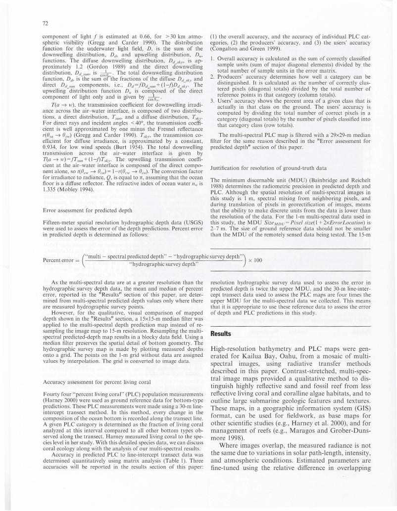
component of light f is estimated at 0.66, for > 30 km atmo­spheric visibility (Gregg and Carder 1990). The distributionfunction for the underwater light field, D, is the SUIll of thedownwelling distribution. Dd , and upwelling distribution, D",functions. The diffuse downwelling distribution, D" skI"> is ap­proximately 1.2 (Gordon 1989) and the direct dcnvnwellingdistribution, D''-'m'" is cosiO . The total downwelling distributionfunction, Dd , is the sum aithe fractions of the diffuse D'C<ky anddirect Dd .wn components. i.e., D,/=fD(f sltll+(I-j)Dd ski" Theupwelling -distribution [unction DII is composed of the' directcomponent of light only and is given by cosiO..,'

T(a ~ 11'), the transmission coefficienl for downwelling irradi­ance across the air-water interface, is composed of two distribu­tions. a direct distribution, Ts"''' and a diffuse distribution. Tsky.

For direct rays and incident angles < 40°, the transmission coeffi­cient is well approximated by one minus the Fresnel reflectancer(O.'I/ -t D.,....) (Gregg and Carder 1990). T.k)", the transmission co­efficient for diffuse irradiance, is approximated by a constant,0.934, for low wind speeds (Burt 1954). The total downwellingtransmission across the air-water interface is given byT(a -t 11')=jTsw,+(I-j)Tsk)" The upwelling transmission coeffi­cient at the air-water interface is composed of the direct compo­nent alone, so 1(0..", -t Dm ) = l-r(Dc,.. -t Dca)' The conversion factorfor irradiance to radiance. Q, is equal to Jr, assuming that the oceanfloor is a diffuse reflector. The refractive index of ocean water II,.. is1.335 (Mobley 1994).

Error assessment for predicted depth

Fifteen-meter spatial resolution hydrographic depth data (USGS)were used to assess the error of the depth predictions. Percent errorin predicted depth is determined as follows:

(I) the overall accuracy, and the accuracy of individual PLC cat­egories, (2) the producers' accuracy. and (3) the users' accuracy(Congalton and Green 1999).

I. Overall accuracy is calculated as the sum of correctly classifiedsample units (sum of major diagonal elements) divided by thetotal number of sample units in the error matrix.

2. Producers' accuracy determines how well a category can bedistinguished. It is calculated as the number of correctly clus­tered pixels (diagonal totals) divided by the total number ofreference points in that category (column totals).

3. Users' accuracy shows the percent area of a given class that isactually in that class on (he ground. The users' accuracy iscomputed by dividing the total number of correct pixels in acategory (diagonal totals) by the number of pixels classified intothat category class (row totals).

The multi-spectral PLC map is filtered with a 29x29-m medianfilter for the same reason described in the IIError assessment forpredicted depth n section of this paper.

Justification for resolution of ground-truth data

The minimum discernable unit (MDU) (Bainbridge and Reichelt1988) determines the radiometric precision in predicted depth andPLC. Although the spatial resolution of multi-spectral images inthis study is I 111, spectral mixing from neighboring pixels. andduring translation of pixels in georectification of images. meansthat the ability to make discrete units from the data is lower thanthe resolution of the data. For the I-m multi-spectral data used inthis study, the MDU Si=eAfDU= Pixel si=e(1 +2xErrorLocatioll) is2-7 m. The size of ground reference data should not be smallerthan the M DU of the remotely sensed data being tested. The 15-m

P ("multi - spectral predicted depth" - "hydrographic survey depth") 00

ercent error = . x I"hydrographlc survey depth"

As the multi·spectral data are at a greater resolution than thehydrographic survey depth data, the mean and median of percenterror, reported in the "Results" section of this paper, are deter­mined from multi-spectral predicted depth values only where thereare measured hydrographic survey points.

However, for the qu;:l1itative. visual comparison of mappeddepth shown in the "Results" section. a 15x15·m median filter wasapplied to the multi-spectral depth prediction map instead of re­sampling the image map to 15-m resolution. Resampling the multi­spectral predicted-depth map results in a blocky data field. Using amedian filter preserves the spatial detail of bottom geometry. Thehydrographic survey map is made by plotting measured depthsonto a grid. The points on the I-m grid without data are assignedvalues by interpolation. The grid is converted to image data.

Accuracy assessment for percent living coral

Fourty four "percent living coral" (PLC) population measurements(Harney 2000) were used as ground reference data for boltom-typepredictions. These PLC measurements were made using a 30-m line­intercept transect method. In this method. every change in thecomposition of the ocean bottom is recorded along the transect line.A given PLC category is determined as the fraction of living coralanalyzed at this interval compared to all other bottom types ob­served along the transect. Harney measured living coral to the spe­cies level in her study. With this detailed species data, we can discusscoral ecology along with the analysis of our multi-spectral results.

Accuracy in predicted PLC to line-intercept transect data wasdetermined quantitatively using matrix analysis (Table I). Threeaccuracies will be reported in the results section of this paper:

resolution hydrographic survey data used to assess the error inpredicted depth is twice the upper MDU. and the 30-m line-inter­cept transect data llsed to assess the PLC maps are four times theupper MDU for the tnulti·spectral data we collected. This meansthat it is appropriate to use these reference data to assess the errorof depth and PLC predictions in this study.

Results

High-resolution bathymetry and PLC maps were gen­erated for Kailua Bay, Oahu, from a mosaic of multi­spectral Images, using radiative transfer methodsdescribed in this paper. Contrast-stretched, multi-spec­tral image maps provided a qualitative method to dis­tinguish highly reflective sand and fossil reef from lessreflective living coral and coralline algae habitats, and tooutline large submarine geologic features and textures.These maps, in a geographic information system (G IS)format, can be used for fieldwork, as base maps forother scientific studies (e.g., Harney el at. 2000), and formanagement of reefs (e.g., Maragos and Grober-Duns­more 1998).

Where images overlap, the measured radiance is notthe same due to variations in solar path-length, intensity,and atmospheric conditions. Estimated parameters arefine-tuned using the relative difference in overlapping

73

Product of depth(z) and distributionfunction (0)

regions of images. The relative difference in overlap­ping regions improves from 7 to 0.9% in the 488-nmband and from 4 to 0.7% in the 551-nm band, after

Fig. 3 Plot of product of depth (z) and distribution function forlight in water (D), and derivative bands (X;) over sand boltom. Thelinear equation for the relationship in each band (I) is inset in thegraph. The slope is equal to the water-attenuation coefficient (K) inthat band. The intercept is In (L/J-L".), the natural log of bottomradiance minus the deep-water radiance for sand in that band.Greater number of data points are shown by dark grey shading inthe linear regression, while fewer data points are shown as lightershades of grey. The occasional horizonra{ fine on the graph resultsfrom missing data

corrections in the radiative transfer model are applied.The 577-nm band does not display the expected reflec­tance pattern and radiative transfer corrections do notimprove the relative difference at overlapping regions.Due to Rayleigh scattering, the reflectance values inimages at this wavelength decrease instead of increasingwhen the sun is higher in the sky. For this reason, andalso since the water-attenuation coefficients for the 551­and 577-nm bands are the same (Table I), results fordepth and bottom type are predicted using the "differ­encing" method [Eqs. (3) and (5)] on the 488- and 551­nm bands only.

A median of 89% and a mean of 86% accuracy inpredicted depth [2488/55], Eq. (5)] are achieved in watersat depths to 30.5 m within the study area (Fig. 4). Per­cent error in predicted depth is not related to depth(R=0.21). Errors are no greater at shallow depths, forexample. Large errors are present along the boundariesof the sand channel and sand fields. These errors mayresult from shadows cast by steep bathymetric gradientsat low sun-elevation angles.

The radiative transfer model assumes a homoge­neous water column, so large errors in predicted depthnot found along margins may be caused by differencesin water quality. Ocean water quality varies withthe amount of sediment or organic detritus in suspen­sion. In addition, the model assumes that reflectance of

Depth prediction

...

-10 m

-20m -10m

-20m

-20m -10m

....~y = 0.07 x + 8.84 IV/"

,I,(

....y = 0.05 x + 8.00 .€I

.....::".-"••41

.~_J--

8.25

8.00

7.75

X488 750

7.25

7.00

6.75

-30m

8.75

8.50

8.25

XS57

8.00

7.75

7.50

7.25

7.00

-30m

8.258.138.007.86

XS777.757.637.507.387.25

-30 m

Table 2 Estimated or calculated sun-angle dependentor non-wavelength-dependent parameters in physical model

Variable Symbol Details Reference

Distribution coefficient

Ratio of direct to totalirradiance

Downwelling air-watertransmission coefficient

Upwelling water-airtransmission coefficient

Conversion factor,irradiance to radiance

Refractive index of water

D

f

T(a ~ w)

1(0(")1' ~ OClI)

Q

D~Dd+Du

Dd = fDa_sun + = I + f= Da_skaDd sky ~ 1.2D - --'-d _\1111 - cos US"DII = I/cosO,.".0.66

T(a ~ II') =jTwlJ + (l-j)TfkyT~kr=O.934

Tw,;, = 1-1'(01'11 ~ O~'ll')I' = Fresnel rejleclallce1(01'1\" ~ On,) = 1-1'(0,.". ~ O,,/)I' = Fresnel refleclancerr

1.334

Gordon (1989)

Gregg and Carder (1990)

BUrl (1954)

Mobley (1994)

Mobley (1994)

74

Table 3 Error matrix for multi-spectral percent living coral map.Ground reference data (line-intercept transects) are in the <:o/limnsand percent living coral categories are in the roil'S. Overall accu­racy, number of correctly classified ground reference poinLs divided

Reference data

by total number of reference points, is shown. Producers' accuracyis calculated as the diagonals divided by collinln IO((IIs. Division ofthe diagonals by roll' IOllIls resuhs in the users' accuracy

< 15% 15-25% 25-40% 40-75% >75% Sand Total

Classified data < 15% 4 1 0 0 0 0 515-25% 1 2 0 0 0 0 325-40% 0 0 2 0 0 0 240-75% 1 1 3 14 3 0 22>75% 0 0 0 0 5 0 5Sand 0 0 0 0 0 7 7

6 4 5 14 8 7 44

Overall accuracy=(4+2+2+ 14+5+7)/44=77%Producers' accuracy Users' accuracy

< 15%15-25%25-40%40-75%>75%Sand

4/62/42/514/145/87/7

67%50%40°/(1100%63%100%

< 15%15-25%25-40%40-75%>75%Sand

4/52/32/214/225/57/7

80%67%100%64%100%100%

bottom type is the same (or the difference is negligible)in the two spectral bands. Examples of spectra of coral,algae and sand can be found in Hochberg andAtkinson (2000) as well as Holden and LeDrew(1999). Where errors in predicted depth are large, thisassumption about bottom reflectance may be thereason.

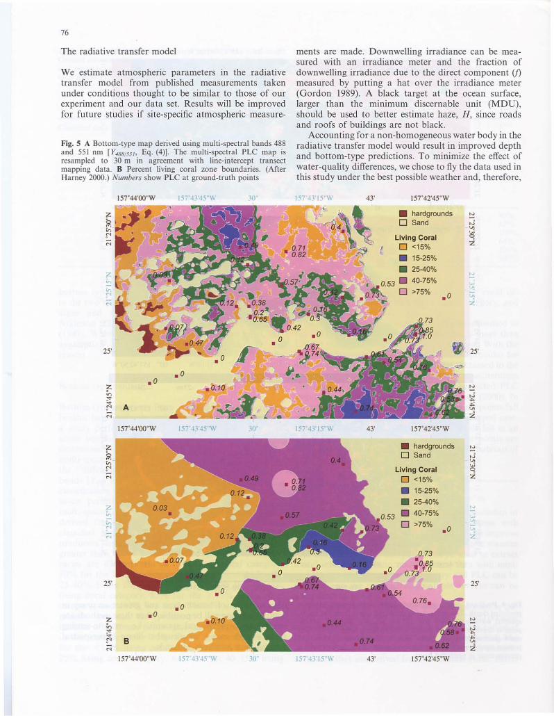
Bottom-type prediction

Bottom-type solutions from multi-spectral data reflectbenthic habitat (Lyzenga 1981; Mumby et al. 1997). Ina study performed by Harney (2000) in Kailua Bay,seven benthic zones were mapped based on PLC asdetermined from 30-m line-intercept transects. Themulti-spectral boltom-type coefficient map made fromthe "differencing" method on the 488- and 551-nmbands [Y488/551, Eq. (3)] is clustered with unsupervisedclassification into seven categories (Fig. 5). Seventy­seven percent overall accuracy is achieved for themulti-spectral PLC map, i.e., 34 of the 44 PLC valuesderived from the 30-m line transects were correctlyclassified. Accuracy for individual classes is shown withproducers' and users' accuracy. Users' accuracies aregreater than the producers' accuracy. Producers' accu­racies are 67% for the < 15% living coral category,50% for the 15-25% living coral category, 40% for the25-40% living coral category, 100% for the 40-75%living coral category, 63% for the > 75% living coralcategory, and 100% for sand. There is a positive cor­relation between the producers' accuracy and thenumber of reference points (line-intercept transect data)in that category (R = 0.73). Users' accuracies are 80%for the < 15% living coral category, 67% for the 15­25% living coral category, 64% for the 40-75% living

coral category, 100% for the 40-75% living coral ca­tegory, 100% for the> 75% living coral category, and100% for sand.

Some reference points are not correctly classified inFig. SA, and it may appear that this occurs more than77% of the time. However, this is not the case. With thecomplete coverage that multi-spectral data provides formapping, we can resolve more detail than attained in themap based on PLC from 44 transect measurementsalone (Fig. 5B). This detail is why the predicted PLCmap looks different from the map in Harney (2000). Inour predicted PLC map, most of the reference points fallwell within or on the boundaries of their mapped cate­gories. However, some of the reference points fall in anarea that is narrow (4-5 pixels wide). These points arealong the walls of the sand channel where the habitats ofPLC can change over a small area.

Discussion

By improving our understanding of the relationship ofcoral reefs ecosystems and sedimentary systems withlocal and global environmental controls, we can improveefforts to manage these systems. The radiative transfermethods described in this paper can be used to extractuseful information from multi-spectral data with mini­mal in situ measurements. Bathymetry and PLC can bemapped and the results from multiple surveys can becompared.

The solutions for depth and boltom type used in thispaper are tested on two bands (488 and 557 nm) becausewe are working with data from a sensor that collectedthree bands and the third (577 nm) was not useful. Theresults mapped for depth and boltom type are remark­able since they are derived from two bands alone. Belter

75

157"44'00"W 50" 45" 157'43'IO"W 30" 25" 20" IS" 157 43'10"W 00" 157'42'50"W;z:

, , ,~

0 - ..;'" ~~

'"f' 0N. .. :2;z: ~

0 ,J

'" U>c' 0N :i

05" -05"

;Z:. -~

'" 'i~

;,- vif' U>M :i

I 57"44'00"W 50'" 45" 15T43'40"W 30" 25" 2{)" 15" 157 43'1O"W 00" I 57"42'50"W

;z: ~0- - ..;'" ~~

'"f' 0N· .. :i

;z: '0Co

~

v-.. -'-'!0' SN Z

05" 05"

;Z:. -~

'" 'i~

?i viU>

N :iI 57"44'00"W 50' 45" 15743'40"W 30" 25" 20" 15" 157 43'1O"W 00" 157'42'50"W.....~ ... .

-3m -6m -9m -12m -15m -18m -21m -24m

'"U>

o:i

·05"

I57"44'00"W

0'05"·-

50" 45" 15T43'10"W"I ; I '

30" 25" 15" 15T43'10"W, , 00" 157'42'50"Wi I

N

157'44'00"W 50" 45" 157'43'40"W 30" 25" 20" 15" 157 4.l'IO"W 00" 157"42'50"W

0-5% 6-10% 11-15% 16-20% 21-25% 26-30% 31-35% >35%

Fig. 4 Predicted depth, measured depth, and percent error inpredicted depth. Top panel shows predicted depth from the multi­spectral wavelengths 488 and 551 om [Z488{55h Eq. (3)]. Middlepanel is depth determined from a USGS hydrographic survey. Themulti-spectral predicted depth map is resampled to 15 m, thepost ian resolution of the hydrographic survey data. Bollom pane! ispercent error in predicted depth

discrimination of bottom type and greater accuracy In

depth prediction will be possible when these methods areapplied to hyperspectral systems, i.e., remote-sensingsystems with many wavelengths. Some hyperspectralsystems have hundreds of bands.

76

The radiative transfer model

We estimate atmospheric parameters in the radiativetransfer model from published measurements takenunder conditions thought to be similar to those of ourexperiment and our data set. Results will be improvedfor future studies if site-specific atmospheric measure-

Fig. 5 A Bottom-type map derived using multi·spectral bands 488and 551 om [Y48815'1> Eq. (4)]. The multi-spectral PLC map isresampled to 30 m in agreement with line-intercept transectmapping data. 8 Percent living coral zone boundaries. (AfterHarney 2000.) Numbers show PLC at ground-truth points

ments are made. Downwelling irradiance can be mea­sured with an irradiance meter and the fraction ofdownwelling irradiance due to the direct component (f)measured by putting a hat over the irradiance meter(Gordon 1989). A black target at the ocean surface,larger than the minimum discemable unit (MDU),should be used to better estimate haze, H, since roadsand roofs of buildings are not black.

Accounting for a non-homogeneous water body in theradiative transfer model would result in improved depthand bottom-type predictions. To minimize the effect ofwater-quality differences, we chose to fly the data used inthis study under the best possible weather and, therefore,

J57°44'()()"W 157 ·n'45"\\ 10" 157 ·0'15"\\ 43' 157°42'45"W

~) 25'

,".'"

.0 ~

z

• hardgroundso Sand

Living Coral0<15%

• 15-25%

• 25-40%, 0.53. 40-75%

.,p.~ 0 >75%

(

('

.0.0

25'

157°42'45"W43'

157 4.ns w 43' J57°42'45"W

• hardgrounds ~

o Sand NU>

living Coral '"qo <15% z

• 15-25%

• 25-40%

• 40-75%~

~

0>75%~

.0 :;;Z

0.73•• 0.85

0.73 1.0

25'

30'

11f157 ·D'4,5"\\'

157 -B'4S"W

.0

B

157°44'OO"W

157°44'()()"W

25'

77

Table 4 Area (in m2) and percent of study area covered by near­

shore hardgrounds. sand. and the percent living coral categories

Fig. 6 Predominant depth and mean slope for PLC categories.Predominant depth, in meters, is taken as the peak of the histogramfor depth in that category, and median and maximum slopes are indegrees for coral cover categories. hardgrounds. and sand

-12

-14

o

-16

-4

-2

<15%living hardcoral grounds

>75% 40-75% 25-40% 15-25%living living living livingcoral coral coral coral

r /'

/ _\c- -

I

/- -

I -[=:J Predominant depth

- ~Slope

sand

2

4

o

8

10

12

the day of data collection, so bottom-type coefficientsfrom multiple days can be compared. Statistical reportsof quantitative spatial change in marine sedimentary andliving environments derived from multi-spectral datacan be monitored and correlated to climate and an­thropogenic activity, which is useful to managers ofcoastlines.

With predicted depth maps made from multi-spectraldata, novel insights and analyses of ocean floor geologyand ecology are possible: for example, maps of reefslope. From these maps, we can begin to analyze therelationship of slope to PLC (Fig. 6). The total areacovered by the PLC categories can be assessed (Table 4).Finally, with detailed ecological ground control data(Harney 2000) and a good understanding of the geo­logical dynamics in Kailua Bay, correlations amonghabitat types and coral and algal species to depth, slope,and coverage area can be made.

The> 75% living coral category is the most spatiallyabundant coral category, making up 25% of the areastudied, about 0.9 km'- Covering 12 and 15% of thePLC map, respectively, the < 15% living coral and 25­40% living coral categories are the next most extensive

Whereas there are other ways of producing bathymetricmaps, doing so lIsing multi-spectral data is still a viablealternative. In general, mapping large areas quickly withspecific survey objectives using multi-spectral sensorscan be cheaper than hyperspectral sensors because theequipment costs are lower and the data reduction costsare less. However, advances in technology are makinghyperspectral data increasingly cost effective.

Shallow depths do not curtail data collection inmulti-spectral remote sensing to map bathymetry as withdepth-mapping mechanisms aboard ships. There iscomplete and extensive coverage when mapping depthwith multi-spectral data, unlike other forms of depthsurveys that only cover a small area or leave out largesections of the study site (e.g., hydrographic surveys,LIDAR).

Depth prediction

ocean conditions. On the day we collected the multi­spectral data, the water was clear in most of Kailua Bay.Even under these conditions, divers noted plumes ofsuspended sediment in portions of the bay.

Over most of the mapped area, the water was clear,and the radiative transfer methods and multi-spectralwavelengths worked well to predict depth and PLC. Inthose areas where the water column had suspendedsediment (and at shallow depths), a combination ofshorter wavelengths will perform better to predict depthand bottom type. Shorter wavelengths with increasedwater attenuation will be less affected by scattering fromparticles in the water (Mobley 1994). The ability to usedifferent combinations of wavelengths in the solutionsfor depth and bottom type based on the water qualityand depth in the study area is one reason why betterpredictions are possible where more wavelengths areavailable, such as with hyperspectral systems.

Some independently measured depth data are neces­sary to run the radiative transfer model. At least threegeoreferenced depth points over sand areas and at leastanother three points over known habitats on the reef areneeded. The three-point minimum allows for linear re­gressions of the derivative channels, Xi, to measureddepth so we can determine water-attenuation coeffi­cients. Points where depth is measured (with latitude andlongitude) can also be used to georegister the multi­spectral image mosaic.

Percent living coral Category Percent ofstudy area

Area(m')

Maps of PLC made from multi-spectral data using ra­diative transfer methods described in this paper can beused as baseline maps for coral reefmonitorillg. RegularPLC mapping will provide information on how reefschange through time. The radiative transfer model cor­rects for sun-angle dependent parameters, and atmo­spheric and water quality variables are determined for

Nearshore hardgroundsSand< 15% living coral15-25% living coral25-40% living coral40-75% living coral> 75% living coral

23812315725

76.7371,569,335493,977123.939602,851290,670924,777

78

o P. lobata encrusting

o P. lobata massive

o P. lobata plate

D M. venvcosa encrusting

I[J M. venvcosa plate

• M. patula encrusting

• M. patula plate

l. n n n

12

10

1l 8c....,c~ 6D«

4

2

>75% 40-75% 25-40% 15-25% <15%

Living Coral

o

Fig. 8 Abundance of coral morphologies for Porites /obara,MOllripora I'crrucosa, and MOlltipora paw/a species in PLCcategories. (Arter Harney 2000)

A map of the slope for every pixel in the multi­spectral mosaic was generated from the predicted depthmap. Analyzing the maps of slope and bottom type, wefind that gentle slopes (mean of 5°, maximum 42°) arefound in the most prolific and least prolific living coralcategories (> 75 and < 15% living coral). The middlePLe categories exhibit steeper slopes, averaging 11°(maximum 60°). We present two hypotheses for thisrelationship among PLC and slope.

The first hypothesis is that the relationship betweenslope and PLC is based on the underlying topographyon which a coral habitat grows. 1n other words, slopeappears to be the inhibiting factor to PLC cover. Thesecond hypothesis is that the relationship between slopeand PLC is a function of the large-scale rugosity of agiven coral reef habitat. Theses two hypotheses can betested in the future. In the following paragraphs, thehypotheses are described in more detail.

There is ecological support of the first hypothesis,that basement topography is the reason we see the> 75and < 15% living coral categories on gentle slopes. Themost abundant coral species in the > 75% living coral

P. fobafa

• P. compressa

• P. meandrina

living Coral

o

2·

8

10

12 1 -------------;;;;:::==::::;-]OM. palu/a

o M. verrucosa

Fig. 7 Abundance of coral species in PLC categories. [Abundanceis an average. It is the number of occurrences (counl) of a givenspecies divided by the number of transects in thai calegory.] (ArterHamey 2000)

categories. With spatial areas of less than 10%, thenearshore hardgrounds, 15-25% living coral, and 40­750/0 living coral categories are the least spatiallyabundant. Sand and fossil reef hardgrounds make upalmost 40% of the study area and have the most ex­tensive depth range to 30 m.

Throughout Kailua Bay (i.e., in all PLC categories),MOlllipora palUla occurs the most (Fig. 7; Harney 2000).This encrusting coral species (Fig. 8) is usually foundgrowing among other corals (Fielding and Robinson1993; Russo 1994), which accounts, in the line-intercepttransect data, for why the counts of this species aregreatest. M. paw/a is used as the species for comparisonin all abundance ratios reported in the following dis­cussIOn.

Abundance is calculated as the number of occur­rences (count) of a given coral species divided by thenumber of transects in that category. It is interesting,however, that M. patu/a is recorded as being commonin shallow water (below 3 m) (Fielding and Robinson1993; Russo 1994), but in Kailua Bay this species isfound throughout the depth range of the study area(Harney 2000). Coral reef habitats in Kailua Bay arefound in depths to 23 m, with about the same stan­dard deviation in depth in all habitats (mean ,,= 4)(Table 5).

Table 5 Minimum and maximum depth (in m) and standard deviation or depth range for percent living coral categories, hardgrounds,and sand

Ollegory Minimum Maximum Standard deviation Predominant Mean Maximumdepth depth or depth depth slope slope(m) (m) (s) (m) (') (')

Hardgrounds -6.0 -19.0 1.2 -7 5 35< 15% living coral cover -4.6 -19.8 3.9 -7 and -13 to -15 6 4015-25% living coral cover -1.4 -23.8 5.0 -6 II 6025-40% living coral cover -1.1 -22.6 4.0 -t2 II 4740-75% living coral cover -0.6t -22.7 3.6 -10 10 55> 75% living coral cover -2.9 -22.6 3.7 -II to -16 6 42Sand -0.94 -30.5 12.1 -15to-25 3 46

category is P. lobara which does well on well-lit, gentlereef slopes (Fielding and Robinson 1993; Russo 1994).In contrast, P. meandrina is the most abundant species inthe < 15% living coral category. This coral species iscommonly found in shallow waters where there arestrong currents or wave action (Fielding and Robinson1993; Russo 1994). Such shallow, wave-eroded reefplatforms have gentle slopes.

However, there is a bimodal depth distribution in the< 15% living coral category. One area where we find the< 150/0 living coral category is in the P. meandrina­dominated, wave-eroded, nearshore, shallow « 7-m)habitat mentioned above. The second < 15% livingcoral cover habitat is found in deep water (13-15 m),north of the sand channel. Since P. l1leandrina are thefirst to colonize (Fielding and Robinson 1993; Russo1994), the high occurrence of P. l1leandrina in deep watermay be evidence of succession. That is, the rehabitationof coral from a previously more prolific growth statethat may have been destroyed or damaged by a signifi­cant event such as large wave stress or human activity.

The middle PLC categories are found in two generalareas: (I) along the slopes of the sand channel, and (2)north and south of the sand channel on spur-and-groovecoral reef fealures. The water-incised sand channel wallsand spur-and-groove geomorphology create steepbathymetric slopes. This first hypothesis suggests thatlhese middle PLC categories are less prolific than the> 75% living coral category because they are found onthese steep geological gradients in the Bay.

The second hypothesis suggests that the slopes are aninherent quality of the PLC habitat, i.e., the slope is ameasure of the topography of the habitat. We explainthat slopes are gentle in the> 75% living coral habitatbecause, in these habitats, corals are prolific and havefilled in all available space laterally and horizontally. Afully grown and filled-in coral garden has an overallgentle slope on its surface.

The < 15% living coral habitats exhibit gentle slopesdue to erosion of topography. This erosion occurs eitherdue to constant wave activity on the shallow reef plat­form or due to periodic large-scale events. Erosion clearsout any large coral colonies that might cause steepbathymetric gradients. Corals in these habitats may below-lying and encrusting forms or small colonies, likethose formed by P. l1leandrina species.

In the middle PLC habitats, coral growth has notcompletely filled in the three-dimensional spaces on thereef, i.e., there are still spaces in the bathymetry of thereef habitat. This results in steep slopes between largecoral colonies or communities of clustered colonies, forexample.

The low producers' accuracy in some PLC categoriesis a result of the small number of transect referencepoints in those categories. The more important cate­gorical accuracy estimate is the users' accuracy as thisdetermines lhe probability of a user going to a givenplace on the bottom-type map and finding a particularPLC there. All users' accuracies are improved over the

79

producers' accuracies, except the 40-75% living coralcategory. There are the most ground truth points plottedwithin this category that should have been allocated toother categories (data in the row of the error matrix,category 40-75%). This is because the details of othercategories within the 40-75% category were lost duringthe resampling of the multi-spectral image to 30-m res­olution to fit the line-transect data resolution.

Bottom reflectance, A (see Appendix), can be directlysolved for, instead of solving for bottom-type coeffi­cients, by using the multi-spectral predicted depth, :, ordepth measured by other means, in the radiative transfermodel (Eq. A2). This is useful since reflectance mea­sured with a field radiometer can be used to train su­pervised classification of predicted bottom reflectancemulti-spectral maps. Reflectance spectra for coral reefsfrom field radiometer measurements are being made(Holden and LeDrew 1999; Hochberg and Atkinson2000) and may become available in spectral libraries inthe future. The use of radiometer-measured coral reefreflectance to train remotely sensed bottom albedo willbe particularly useful with hyperspectral data wheremany wavelengths of reflected sunlight (in contrast tothree in this study) are measured. The greater number ofbands measured in hyperspectral remote sensing gives aspectrum of sensor-measured reflectance (in multiplelayers of digital band maps) to train with a spectrum offield radiometer-measured reflectance. Hence, the shapeof the reflectance spectrum for each bottom type as wellas the strength of the reflectance signal in a given bandare used to solve for the bottom type.

Although field-measured reflectance to perform su­pervised classification on remotely sensed data has beenin use on land for some time, this approach in marineenvironments is still in its infancy. One reason is that theminimum discernable unit for multi-spectral data islarger than the size of individual coral species, so spectrashould be a measure of habitat type rather than speciesuntil greater resolution is achieved. In addition, this ap­proach has not been lIsed extensively in marine envi­ronments, because the correction of remotely sensed datafor the effects of the ocean is in an early stage of devel­opment. However, researchers are working on measuringspectral reflectance of habitats with field radiometers(e.g., Holden and LeDrew 1999), and sensors able toacquire greater resolution will be developed in the future.

Conclusions

I. The radiative transfer model and estimated parame­ters used in this paper are sufficient to normalizemulti-spectral images in a mosaic to one another andcan be used with any passive airborne remote sensingdigital data.

2. Bathymetry and PLC are appropriately mapped fromtwo bands of multi-spectral data (488 and 551 nm)using the "differencing" method we present in thispaper.

80

Appendix A: Significant symbols

3. Spatial change in depth and PLC can be mappedthrough time with multi-spectral data using themethods described in this paper and if additionalmulti-spectral data sets are collected at differentdates.

4. The greatest PLC habitats are found on reef topswhere gentle slopes are observed. Gentle slopes arealso observed in the least PLC habitats. In contrast,the medium PLC habitats are associated with steeperreef slopes.

(A I)

(A2)

Radiance measured at the multi-spectraldetector [Eqs. (A3) and (M)]('W m-2 nm- I sr- I )

Radiance of the ocean('W m-2 nm- I sr- I )

Refractive index of waterConversion factor for irradiance toradianceIrradiance reflectance of the ocean (sr- I

)

Transmission coefficient for downwel­ling irradiance across the air-waterinterfaceTransmission coefficient for the directcomponent of downwelling irradianceacross the air-water interfaceTransmission coefficient for the diffusecomponent of downwelling irradianceacross the air-water interfaceSnell transmission coefficient for radi­ance to the camera across the water-airinterfaceWater-attenuation coefficient (m- I

)

Optical extinction coefficients for aero­sol, Rayleigh and ozone scattering forthe distance from the ocean surface tothe sensor (km- I

)

Optical extinction coefficients for aero­sol, Rayleigh and ozone scattering forthe atmosphere from space to earth(km- I )

Solar zenith angle in airSolar zenith angle in waterCamera zenith angle in airCamera zenith angle in water

'f."1I1J

R _ £,,(z)'" - £d(Z)

For a given wavelength, }'i.. the reflectance just beneaththe water surface, R(O-), can be written as

Following Philpot (1989), the irradiance reflectance,R(=), is the ratio of upwelling irradiance to downwellingirradiance:

K

R~

T(a ~ IV)

where bottom albedo, A, is the value of R just above thebottom; R.. is the value of R (0-) for an infinitely deepocean; K is a water-attenuation coefficient; and D is thedistribution function for the underwater light field.

In a comprehensive formula that includes transmis­sion across the air-water interface, atmospheric effects,solar illumination, and the conversion of irradiance toradiance, the upwelling radiance measured at the multi-

Appendix B: Radiative transfer theory

r'A, r'R, r'oz

OsaO:i\I'OcaDc1l'

11 11,

Q

Irradiance reflectance (albedo) of theocean bottom (sr- I

)

Atmospheric transmittance from spaceto the ocean surface (0 to ~)

Atmospheric transmittance from theocean surface to the multi-spectralsensor (0 to he)Distribution function for the underwa­ter light fieldDistribution function for the downwel­ling underwater light fieldDistribution function for the diffusecomponent of the downwelling under­water light fieldDistribution function for the directcomponent of the downwelling under­water light fieldDistribution function for the upwellingunderwa ter ligh t fieldDownwelling irradiance (W m-2 nm- I

)

Fraction of direct sunlight to totalsunlight in the incident radiation trans­mitted through the air-water interfaceExtraterrestrial irradiance corrected forearth-sun distance and orbital eccen­tricity ('W m-2 nm- I)

Path irradiance due to scattering byparticles in the atmosphere between theocean surface and the airplane(W m-2 nm- I )

Ocean bottom radiance(W m-2 nm- I sr- I )

D

H

A

D"

Fa

Acknowledgements This research was funded by the USGS Coastaland Marine Geology Program, the University of Hawaii SeaGrant. and the NASA Eanh System Science Fellowship (NASAreference number ESS/99-0000-0263). Many thanks to Jodi Har­ney, Eric Grossman, and John Rooney for shared data and fieldassistance. The orthoreClified aerial photographs lIsed to georectifythe multi-spectral images were made available by Melanie Coyneand Zoe orcross. TerraSystems Inc. used their multi-spectralsensor. the Application Specific Multi-Spectral Camera System. 10collect the data used in this study and provided much assistanceand advice. Additional thanks to Scott Rowland of the Hawai'iInstitute of Geophysics and Planetology for editorial help andscientific advice.

81

R)'(0-) = £,(0-)

(_.. Q

h,

14(0')= ~~;) 1(8~ .... 8~)

/:.," :

haze (If)

diffuse downwelling

irradiance, Ef'

f

\ \ \! '- 0 WATER £,(0-) = £,(O')T(aU!, \ \ f f

transmitted direct and diffuse i !downwelling irradiance ;j, i ~ scattering in the ocean

( . ,distributionfuncLion. D • .' \1 bottom reflectance (A)

Fig. 9 Components of theradiative transfer model

References

if L d , the radiance measured at the multi-spectral de­tector, is defined as

(A4)

(AS)

Bainbridge SJ, Reichelt RE (1988) An assessmenl of ground tru­thing methods for coral reef remote sensing data. Proc 6lh IntCoral Reef Symp 2:439-444

Burt WV (1954) Albedo over wind-roughened water. J MeteorolII :283-290

Congalton RG, Green K (1999) Assessing the accuracy of remotelysensed data: principles and practices. Lewis, Boca Raton,137 pp

Coyne MA, Fletcher CH, Richmond BM (1999) Mapping coastalerosion hazard areas in Hawai'i: observations and errors.J Coast Res 28:171-184

Ellerman L (1968) UV, visible and IR attenuation for altitudes to50 km. 1968. National Technical Information Service. Spring­field, 57 pp

Fielding A, Robinson E (1993) An underwater guide to Hawai'i.University of Hawai'i Press, Honolulu, 156 pp

h C T(o-w) ,(0 _0) L . I b d·were 0 = QIIC' CD; b IS t le oltom-type fa l-

ance; L". is the radiance of the water column; and g isdefined as the product of the water-attenuation coeffi­cient, K, and the distribution function, D, given byg= KD.

the transmission coefficient for upwelling radiance acrossthe water~air interface, and 00 1" is the incident, zenithbottom-reflecta nce angle (ell' = camera pa th in wa ter). Qisa conversion factor for irradiance to radiance, which forour calculations can be taken to have the value n, and 1111" isthe index of refraction for waler.

Equation (A3) can be written in the simplified form

111 which he is the height of the camera above the seasurface and £jO +) is the total downwelling irradiance,attenuated by the atmosphere, just above the oceansurface (Fig. 9). £,,(0 +) IS gIven by £,,(0+) =

(cos O,.oFo(i)AT-")/j where FoCi) is extraterrestrial irradi­ance corrected for earth-sun distance and orbital ec­centricity (Gregg and Carder 1990) and! is the fractionof total downwelling light due to the direct component,i.e. the ratio of irradiance due to sunlight to irradianceof sunlight plus skylight. AT 0' the atmospheric trans­mission for the height of the atmosphere (from the oceansurface 10 space), involves the exponent of optical ex­tinction coefficients, r'A. T'R, and T'oz. for aerosol,Rayleigh, and ozone scattering and absorption in the

[r' +r' +,' J/atmosphere, respectively. Ara= exp- A R 0=

COS Osa where 0S(I is the incident, zenith sun angle (sa =

sun in air).H is path radiance due to scattering by particles in the

atmosphere between the ocean surface and the airplane.AT c is the atmospheric transmittance back to the cam­era~ With optical extinction coefficients for the distancefrom the ocean surface to the altitude of the airplane

-i'A + 'R + 'ad/cos 0 O·(0 to he.), AT..J:= exp C(l where ClI IS

the transmitted, zenith bottom-reflectance angle(ca=camera path in air).

T(a -? IV) is the transmission coefficient for downwel-I· . d· h·· f ,(0 -0 ) .II1g IITa lance across t e all'~water Inter ace. rw j r" IS

II~.

spectral camera, L II • for a given wavelength, Ai, is writtenas:

82

Gordon H R (1989) Dependence of the diffuse reflectance of naturalwaters on the sun angle. Limnol Oceanogr 34: 1484--1489

Gordon HR. Brown OB (1973) Irradiance reflectivity of a flatocean as a function of its optical properties. Appl Opt 12: 1549­1551

Gordon HR, Brown OB (1974) Influence of depth and albedo onthe diffuse reflectance of a flat homogeneous ocean. Appl Opt13:2153-2159

Gordon HR, McCluney WR (1975) Estimation of the depth ofsunlight penetration in the sea for remote sensing. Appl Opt14:413-416

Green EP, Mumby PJ, Edwards AJ, Clark CD (1996) A review ofremote sensing for the assessment and management of tropicalcoastal resources. Coast Manage 24: 1-40

Gregg WW, Carder KL (1990) A simple speclral solar irradiancemodel for cloudless maritime atmospheres. Limnol Oceanogr35:1657-1675

Harney IN (2000) Carbonate sedimentology of a windwardshoreface: Kailua Bay, Oahu, Hawaiian Islands. PhD Thesis,Department of Geology and Geophysics, University of Hawai'i,Honolulu, 232 pp

Harney lN, Grossman EE, Richmond 8M, Fletcher CH (2000)Age and composition of carbonate shoreface sediments, KailuaBay, Oahu, Hawai'i. Coral Reefs 19:141-154

Hochberg El. Atkinson Ml (2000) Spectral discrimination of coralreef benthic communities. Coral Reefs 19: 164-171

Holden H, LeDrew E (1999) Hyperspectral identification of coralreef features. Int 1 Remote Sensing 20:2545-2563

Kirk lT (1991) Volume scattering function, average cosines, andthe underwater light field. Limnol Oceanogr 36:455-467

Lee Z, Kendall LC, Hawes SK, Steward RG, Peacock TG, CurtisOD (1994) Model for the interpretation of hyperspectral re­mote-sensing reflectance. Appl OPl 33:5721-5732

Lyzenga DR (1977) Reflectance of a flat ocean in the limit of zerowater depth. Appl Opt 16:282-283

Lyzenga DR (1978) Passive remote sensing technique for mappingwater depth and bottom features. Appl Opt 17:379-383

Lyzenga DR (1981) Remote sensing of bottom reflectance andwater attenuation parameters in shallow water using aircraftand Landsat data. Int 1 Remote Sensing 2:71-82

Maracci G (1985) Results of atmospheric optical measurements attwo sites on the Cape West Coast. In: Channon LV (ed) SouthAfrican Ocean Colour and Upwelling Experiment. Sea Fisher­ies Research Institute, Cape Town, pp 171-175

Maragos JE, Grober-Dunsmore R (eds) (l998) Proceeding of theHawai'i Coral Reef Monitoring Worksh, East·West Center,Honolulu, 334 pp

Maritorena S (1996) Remole sensing of the water attenualion incoral reefs: a case study in French Polynesia. Int 1 RemoteSensing 17: 155-166

Mobley CD (1994) Light and water: radiative transfer in naturalwaters. Academic Press, San Diego, 592 pp

Mumby PJ, Green EP, Edwards AJ, Clark CD (1997) Coral reefhabitat-mapping: how much detail can remote sensing provide?Mar Bioi 130: 193-202

Mumby PJ, Green EP, Clark CD, Edwards AJ (1998) Digitalanalysis of multispectral airborne imagery of coral reefs. CoralReefs 19:59-69

Paredes 1M, Spero RE (1983) Water depth mapping from remotesensing data under generalized ration assumption. Appl Opt22: 1134-1135

Philpot W (1989) Bathymetric mapping with passive multispectralimagery. Appl Opt 28:1569-1578

Russo R (1994) Hawaiian reefs: a natural history guide. LorrainePress, Salt Lake City, 174 pp