Multi-Stage Multi-Objective Solid Transportation Problemfor Disaster Response Operation with Type-2 Triangular

Fuzzy Variables

Abhijit Baidya∗† , Uttam Kumar Bera‡ and Manoranjan Maiti§

Abstract

In this paper, for the first time we formulate and solve multi-stage solid trans-portation problem (MSSTP) to minimize the total cost and time with type-2 fuzzytransportation parameters. During transportation period, loading, unloading costand time, volume and weight for each item, limitation of volume and weight for eachvehicle are normally imprecise and taken into account to formulate the models. Toremove the uncertainty of the type-2 fuzzy transportation parameters from objectivefunctions and constraints, we apply CV-Based reduction methods and generalizedcredibility measure. Disasters are unexpected situations that require significantlogistical deployment to transport equipment and humanitarian goods in order tohelp and provide relief to victims and sometime this transportation is not possibledirectly from supply point to destination. Again, the availabilities at supply pointsand requirements at destinations are not known precisely due to disaster. For thisreason, we formulate the multi-stage solid transportation problems under uncertainty(type-2 fuzzy). The models are illustrated with a numerical example. Finally, gen-eralized reduced gradient technique (LINGO.13.0 software) is used to solve the models.

Keywords: Multi-stage solid transportation problem, type-2 fuzzy variable, CV-based reductionmethods, generalized credibility, goal programming approach.

2000 AMS Classification: 90B06, 90C05, 90C29

1. Introduction

1.1. Literature review and the main work of the research: The transportation problemoriginally developed by Hitchcock [7] is one of the most common combinatorial problems involvingconstraints. The solid transportation problem (STP) was first stated by Shell [8]. Haley [5, 6]developed the solution procedure of a solid transportation problem and made a comparison be-tween the STP and the classical transportation problem. Geoffrion and Graves [19] were the firstresearchers studied on two-stage distribution problem. After that so many researchers(Pirkul andJayaraman [20], Heragu [17], Hindi et al. [21], Syarif and Gen [22], Amiri [23], Gen et al. [24])study two-stage TP. Mahapatra et al. [25] applied fuzzy multi-objective mathematical program-ming technique on a reliability optimization model. A type-2 fuzzy variable is a map from a fuzzy

∗Department of Mathematics, National Institute of Technology, Agartala, Barjala, Jirania,Tripura, India, Pin-

799046, Email: abhijitnita@yahoo.in†Corresponding Author.‡Department of Mathematics, National Institute of Technology, Agartala, Barjala, Jirania,Tripura, India, Pin-

799046, Email: bera uttam@yahoo.co.in§Department of Applied Mathematics with oceanology and computer programming, Vidyasagar University ,

Midnapur-721102, W. B. ,India, Email: mmaiti2005@yahoo.co.in

2

possibility space to the real number space; it is an appropriate tool for describing type-2 fuzziness.The concept of a type-2 fuzzy set was first proposed in Qin et al. [1] as an extension of an ordinaryfuzzy set. Mitchell [10] used the concept of an embedded type-1 fuzzy number. Liang and Mendel[11] proposed the concept of an interval type-2 fuzzy set. Karnik and Mendel [2], Liu [3], Qinet al. [1], Yang et al. [30], Liu et al. [29], Yang et al. [30] worked on type-2 fuzzy set. In theliterature, data envelopment analysis (DEA) technology was first proposed in [12]. Sengupta [22]incorporated stochastic input and output variations; Banker [14] incorporated stochastic variablesinto DEA; Cooper et al. [15] and Land et al. [16] developed a chance-constrained programmingto accommodate the stochastic variations in the data. Qin et al. [4] proposes three noble methodsof reduction for a type-2 fuzzy variable. Here, we present in tabular form a scenario of literaturedevelopment made on transportation problem in Table-1.

Table-1: Some remarkable research works on TP/STPAuthor(s), Ref. Objective Nature Additional function Environments Solution Techniques

Kundu et al. Multi-objective STP Multi-item fuzzy LINGOYang and Feng Single-objective STP fixed charges stochastic Tabu search algorithmKundu et al. Single-objective TP Fixed charge type-2 fuzzy variable LINGOBaidya et al. Single-objective STP Safety factor Fuzzy, Stochastic, Interval LINGO

Gen et al. Single-objective TP Two-stage Deterministic Genetic algorithmsProposed Multi-objective STP Multi-stage Triangular type-2 fuzzy LINGO

In spite of the above developments, there are so many gaps in the literature. Some of these omis-sions which are used to formulate the model with type-2 triangular fuzzy number are as follows:

• So many ([26], [27], [28], [31], [32], [33],) solid transportation problems exist in the litera-ture to minimize the total transportation cost only but nobody can formulate any STP tominimize the total transportation time, purchasing cost, loading and unloading cost at atime.

• In spite of the above developments, very few can minimized the time objective functionwhich involves total transportation time, loading and unloading time at a time.

• Lots of two stage transportation problems ([19]-[25]) exist in the literature where the trans-portation cost is minimized. But nobody formulate and solved a multi-stage multi-itemmulti-objective solid transportation problem to minimize the ”total cost” which involvestransportation cost, purchasing cost, loading and unloading cost and ”total time” whichinvolves transportation time, loading and unloading time.

• Sometimes, the value of the transportation parameters are not known to us precisely but atthat time some imprecise data are known to us. For this reason, lots of researchers solvedso many transportation problems with fuzzy (triangular fuzzy number, trapezoidal fuzzynumber, type-1 fuzzy number, type-2 fuzzy number, interval type-2 fuzzy number etc.)transportation parameters. But nobody solved any multi-stage multi-item multi-objective(cost and time) STP with transportation parameters as type-2 triangular fuzzy number.

• So many STPs are developed in the literature to minimize the total transportation costand time subjected to the supply constraints, demand constraints and conveyances capac-ity constraints, budget constraint, safety constraint etc. but nobody formulated any STPsubjected to the weights constraints and volumes constraints during transportation.

3

In this paper, a multi-item multi-stage solid transportation problem is formulated and solved.Type-2 fuzzy theory is an appropriate field for research. To formulate the model, we considerunit transportation cost, time, supplies, demands, conveyances capacities, loading and unloadingcost and time, volume and weights for each and every item, volume and weight capacities for eachconveyances as type-2 triangular fuzzy variables. The objective functions for the respective trans-portation model is to minimize the total cost and time. To defuzzify the constraints and objectivefunctions, we apply CV-based reduction method. The goal programming approach is used to solvethe multi-objective programming problem. The deterministic problems so obtained are then solvedby using the standard optimization solver - LINGO 13.0 software. We have provided numericalexamples illustrating the proposed model and techniques. Some sensitivity analyzes for the modelare also presented.The paper is organized as follows. Problem descriptions are includes in the section 2. In section 3we briefly introduce some fundamental concepts. The assumptions and notations to construct themodel are put in the section 4. In section 5, multi-stage multi-objective solid transportation modelwith type-2 triangular fuzzy variable is formulated. In section 6, we discuss about the methodologyand defuzzification method that used to solve the model. A numerical example put in the section 7is to illustrate the model numerically. The results of solving the model numerically are put in thesection 8. A sensitivity analysis of the model is discussed in the section 9. In section 9, we discussthe results obtained by solving the numerical example. The comparisons of the work with the earlierresearch are discussed in the section 10. The conclusion and future extension of the research workare discussed in the section 11. The references which are used to prepare this manuscript are put inthe last. In this work, we formulate and solve a multi-stage multi-item solid transportation problemto minimize the total cost and time under type-2 fuzzy environment. The real life applications ofthe research work are as follows:

• Basically to provide some relief to the survived peoples in disaster, we developed our MSSTPmodel. In our paper, we consider all the transportation parameters as type-2 fuzzy variablessince after disaster, it is very difficult to define all transportation parameters precisely. Sincedue to disaster roads, bridges, towers etc. are damaged, thus it is not possible to survivethe peoples smoothly with the help of direct transportation network. This is the reason toformulate an n-stage solid transportation model

• To get the permit of a vehicle is a difficult task for the owner of the vehicle. Some vehiclesare permitted to driver on a particular state or country. This permit restricts us to carry thegoods from one state to another or one country to another. So in the transportation period,it is important to load and unload the goods so many times at the destination centers (thedestination centers are lies between supply points and customers).So to overcome thesetransportation difficulties we can apply this newly developed model.

1.2. Motivations: The motivation for this research dated back to September 2014, the Kashmirregion witnessed disastrous floods across majority of its districts caused by torrential rainfall. TheIndian administrated Jammu and Kashmir, as well as Azad Kashmir, Gilgit-Baltistan and Punjabin Pakistan, were affected by these floods. By September 24, 2014, nearly 277 people in India and280 people in Pakistan died due to the floods and more than 1.1 million were affected by the floods.During this period, it is tedious to send the necessary foods to the survived peoples. For this reason,it is important to impose so many destination centers in between supply point and customers.

4

2. Problem Description:

Disaster (earthquick, flood etc.) is an extra ordinary situation for any country or state and toprovide relief to the survived person which is a risky and tedious task to us. But at that timetransportation is required to serve the foods, clothes etc. to the peoples. Also due to the disas-ter, it is not possible to deliver the necessary things directly to the survived people. It requiredsome destination centers in between source point and survived peoples such that the total cost andtime should be minimized. This also motivated us to formulate a multi-stage multi-objective solidtransportation problem. The exact figure of the survived peoples due to disaster is not known tous exactly. For this reason, the transportation parameters are also remains unknown to us. Sinceall the transportation parameters are not known to us precisely, so we consider the transportationparameters as type-2 triangular fuzzy variables. In this multi-stage transportation network, desti-nation center for stage-1 is reduced to the supply point for stage-2 and destination center for stage-2is reduced to the supply point for stage-3 and similarly the destination center for the stage-(n-1) isconverted to the supply point to the stage-n. The pictorial representation of the multi-stage solidtransportation problem is as follows:

Figure 1. Multi-stage solid transportation network

3. Fundamental Concepts

Definition 1. (Regular Fuzzy Variable)Let Γ be the universe of discourse. An ample field [32] A on Γ is a class of subsets of Γ that isclosed under arbitrary unions, intersections, and complements in Γ.Let Pos : A → [0, 1] be a set function on the amplefield Γ. Pos is said to be a possibility measure[32] if it satisfies the following conditions:(p1) Pos(ϕ) = 0 and Pos(Γ) = 1.(p2) For any subclass {Ai|i ∈ I} of A (finite, counter or uncountable), Pos(

⋃i∈I(Ai)) = Supi∈IPos(Ai)

The triplet (Γ,A, Pos) is referred to as a possibility space, in which a credibility measure [33] isdefined as Cr(A) = 1

2 (1 + Pos(A)− Pos(Ac)), A ∈ A.If (Γ,A, Pos) is a possibility space, then an m-ary regular fuzzy vector ξ = (ξ1, ξ2, ..., ξm) is definedas a membership map from Γ to the space [0, 1]m in the sense that for every t = (t1, t2, ..., tm) ∈[0, 1]m, one has{γ ∈ Γ|ξ(γ) ≤ t} = {γ ∈ Γ|ξ1(γ) ≤ t1, ξ2(γ) ≤ t2, ..., ξm(γ) ≤ tm} ∈ A

When m = 1, ξ is called a regular fuzzy variable (RFV).

5

3.1. Critical values for RFVs. .Definition 2.(Qin et al. [1]) Let ξ be an RFV. Then the optimistic CV of ξ, denoted by CV ∗[ξ],defined as CV ∗[ξ] = Sup{α ∧ Pos{ξ ≥ α}}︸ ︷︷ ︸

α∈[0,1]

, while the pessimistic CV of ξ, denoted by CV∗[ξ], is

defined as CV∗[ξ] = Sup{α ∧Nec{ξ ≥ α}}︸ ︷︷ ︸α∈[0,1]

.

The CV of ξ , denoted by CV [ξ], is defined as CV [ξ] = Sup{α ∧ Cr{ξ ≥ α}}︸ ︷︷ ︸α∈[0,1]

.

Theorem 1. (Qin et al. [1]) Let ξ = (r1, r2, r3, r4) be a trapezoidal RFV. Then we have

(i) The optimistic CV of ξ is CV ∗[ξ] = r41+r4−r3 .

(ii) The pessimistic CV of ξ is CV∗[ξ] = r21+r2−r1 .

(iii) The CV of ξ is CV [ξ] =

2r2−r1

1+2(r2−r1) , if r2 >12

12 , if r2 ≤ 1

2 ≤ r3r4

1+2(r4−r3) , r3 ≤ 12

3.2. Methods of reduction for type-2 fuzzy variables (CV-Based Reduction Methods).Due to the fuzzy membership function of a type-2 fuzzy number, the computation complexity isvery high in practical applications. To avoid this difficulty, some defuzzification methods have beenproposed in the literature (see [6-8]). In this section, we propose some new methods of reductionfor a type-2 fuzzy variable. Compared with the existing methods, the new methods are very mucheasier to implement when we employ them to build a mathematical model with type-2 fuzzy coef-ficients.Let (Γ,A, ˜Pos) be a fuzzy possibility space and ξ a type-2 fuzzy variable with a known secondarypossibility distribution function µξ(x). To reduce the type-2 fuzziness, one approach is to give a rep-

resenting value for RFV µξ(x). For this purpose, we suggest employing the CVs of ˜Pos{γ|ξ(γ) = x}as the representing values. This methods the CV-based methods for the type-2 fuzzy variable ξTheorem 2.(Qin et al. [1]) Let ξ be a type-2 triangular fuzzy variable defined as ξ = (r1, r2, r3; θl, θr).Then we have

(i) Using the optimistic CV reduction method, the reduction ξ1 of ξ has the following possibilitydistribution:

µξ1(x) =

(1+θr)(x−r1)

(r2−r1+θr(x−r1)) , if x ∈ [r1,r1+r2

2 ](1−θr)x+θrr2−r1(r2−r1+θl(r2−x)) , if x ∈ [ r1+r2

2 , r2](−1+θr)x−θrr2+r3r3−r2+θr(x−r2) , if x ∈ [r2,

r2+r32 ]

(1+θr)(r3−x)r3−r2+θr(r3−x) , if x ∈ [ r2+r3

2 , r3]

(ii) Using the pessimistic CV reduction method, the reduction ξ2 of ξ has the following possi-bility distribution:

µξ2(x) =

x−r1

r2−r1+θl(x−r1) , if x ∈ [r1,r1+r2

2 ]x−r1

r2−r1+θl(r2−x) , if x ∈ [ r1+r22 , r2]

r3−xr3−r2+θl(x−r2) , if x ∈ [r2,

r2+r32 ]

r3−xr3−r2+θl(r3−x) , if x ∈ [ r2+r3

2 , r3]

6

(iii) Using the CV reduction method, the reduction ξ3 of ξ has the following possibility distri-bution:

µξ3(x) =

(1+θr)(x−r1)

r2−r1+2θr(x−r1) , if x ∈ [r1,r1+r2

2 ](1−θl)x+θlr2−r1r2−r1+2θl(r2−x) , if x ∈ [ r1+r2

2 , r2](−1+θl)x−θlr2+r3r3−r2+2θl(x−r2) , if x ∈ [r2,

r2+r32 ]

(1+θr)(r3−x)r3−r2+2θr(r3−x) , if x ∈ [ r2+r3

2 , r3]

3.3. Generalized credibility and its properties. Suppose ξ is a general fuzzy variable withthe distribution µ. The generalized credibility measure Cr of the event {ξ ≥ α} is defined by

Cr({ξ ≥ α}) = 12 (Supx∈Rµ(x) + Supx≥rµ(x)− Supx<rµ(x)), r ∈ R.

Therefore, if ξ is normalized, it is easy to check that Cr(ξ ≥ α) + Cr(ξ < α) = Supx∈Rµξ(x) = 1;

then Cr coincides with the usual credibility measure. The concept of independence for normalizedfuzzy variables and its properties were discussed in [35]. In the following, we also need to extendindependence to general fuzzy variables. The general fuzzy variables ξ1, ξ2, ξ2..., ξn are said to bemutually independent if and only if Cr{ξi ∈ Bi, i = 1, 2, ...n} = Min1≤i≤nCr{ξi ∈ Bi} for anysubsets Bi, i = 1, 2, ...n of RLike the α-optimistic value of the normalized fuzzy variable [36], the α-optimistic value of generalfuzzy variables can be defined through the generalized credibility measure. Let ξ be a fuzzy vari-able (not necessary normalized). Then ξSup(α) = Sup{r|Cr{ξ ≥ r} ≥ α}, α ∈ [0, 1] is called the

α-optimistic value of ξ, while ξinf = Inf{r|Cr{ξ ≤ r} ≥ α}, α ∈ [0, 1] , is called the α− pessimisticvalue of ξ.Theorem 3. (Qin et al. [1]) Let ξi be the reduction of the type-2 fuzzy variableξi = (ri1, r

i2, r

i3; θl,i, θr,i)

obtained by the CV reduction method for i = 1, 2, ...n. Suppose ξ1, ξ2, ..., ξn are mutually indepen-dent, and ki ≥ o for i = 1, 2, ...n.Case-I: If α ∈ (0, 0.25], then eqnarray Cr{

∑ni=1 kiξi ≤ t} ≥ α is equivalent to

n∑i=1

(1− 2α+ (1− 4α)θr,i)kiri1 + 2αkir

i2

1 + (1− 4α)θr,i

Case-II: If α ∈ (0.25, 0.50], then eqnarray Cr{∑ni=1 kiξi ≤ t} ≥ α is equivalent to

n∑i=1

(1− 2α)kiri1 + (2α+ (4α− 1)θl,i)kir

i2

1 + (1− 4α)θl,i

Case-III: If α ∈ (0.50, 0.75], then eqnarray Cr{∑ni=1 kiξi ≤ t} ≥ α is equivalent to

n∑i=1

(2α− 1)kiri3 + (2(1− α) + (3− 4α)θl,i)kir

i2

1 + (3− 4α)θl,i

7

Case-IV: If α ∈ (0.75, 1], then eqnarray Cr{∑ni=1 kiξi ≤ t} ≥ α is equivalent to

n∑i=1

(2α− 1 + (4α− 3)θr,i)kiri3 + 2(1− α)kir

i2

1 + (4α− 3)θr,i

3.4. Goal programming Method. .The goal programming method is used to solve the multi-objective programming problem (MOPP).A general MOPP is of the following form: Find the values of L decision variablesx1, x2, ..., xLwhich minimizes

F (x) = (f1(x), f2(x), ..., fQ(x))T

subject tox ∈ X(3.1)

Where, X = {x = (x1, x2, ..., xL) such that gt(x) ≤ 0, xl ≥ 0, t = 1, 2, ..., T ; l = 1, 2, ..., L} andf1(x), f2(x), ..., fQ(x) are Q(≥ 2) objective functions.The different steps of the goal programming method are as follows:Step-1: Solve the multi-objective programming problem (1) as a single objective problem usingonly one objective at a time ignoring the others, and determine the ideal objective vector, sayfmin1 , fmin2 , ..., fminQ .Step-2: Formulate the following GP problem using the ideal objective vector obtained is Step-1,

Min{Q∑q=1

[(d+q )p + (d−q )p]}

1p

subject to fq(x) + d+q − d−q = fminq , d+

q ≥ 0, d−q ≥ 0, d+q d−q = 0(q = 1, 2, ..., Q), for all x ∈ X.

Step-3: Now, solve the above single objective problem described in Step-2 by GRG method andobtain the compromise solution.

4. Notations and assumptions for the proposed model

(i) C1ijk1q

, C2jkk2q

, Cnlmknq = Fuzzy unit transportation cost is to transport the q-th item fromi-th plant to j-th DC by k1-th vehicle, j-th plant to k-th DC k2-th vehicle and l-th plantto m-th customer kn-th vehicle respectively.

(ii) t1ijk1q, t2jkk2q

, tnlmknq = Fuzzy unit transportation time is to transport the q-th item fromi-th plant to j-th DC by k1-th vehicle, j-th plant to k-th DC k2-th vehicle and l-th plantto m-th customer kn-th vehicle respectively.

(iii) x1ijk1q

, x2jkk2q

, xnlmknq, xnulk(n−1)q

, xnlmknq = Unknown quantities which is to be transported

from i-th plant to j-th DC of q-th item by k1-th vehicle for stage-1, j-th plant to k-th DCof q-th item by k2-th vehicle for stage-2, u-th plant to l-th DC of q-th item by k(n−1)-thvehicle for stage-(n− 1), and l-th plant to m-th customer of q-th item by kn-th vehicle forstage-n respectively.

8

(iv) PC = Fuzzy purchasing cost of q-th item at i-th source.

(v) LO1

i , LO2

j , ..., LOn

l = Fuzzy loading cost at i-th plant of stage-1, j-th plant of stage-2 andl-th plant of stage-n respectively.

(vi) UD1

j , UD2

k, ..., UDn

m =Fuzzy unloading cost at j-th DC of stage-1, k-th DC of stage-2 andm-th customer of stage-n respectively.

(vii) ˜LTO1

i , ˜LTO2

j , ..., ˜LTOn

l = Fuzzy loading time at i-th plant of stage-1, j-th plant of stage-2and l-th plant of stage-n respectively.

(viii) ˜UTD1

j , ˜UTD2

k, ..., ˜UTDn

m =Fuzzy unloading time at j-th DC of stage-1, k-th DC of stage-2and m-th customer of stage-n respectively.

(ix) y1ijk1q

=

{1, if x1

ijk1q> 0

0, otherwise, y2

jkk2q=

{1, if x2

jkk2q> 0

0, otherwise, ynlmknq =

{1, if xnlmknq > 0

0, otherwise

5. Formulation of solid transportation problem with transportation parametersas type-2 triangular fuzzy variables

Let us consider ′I ′ supply points (or sources), ′J ′ destination centers, K1 conveyances for stage-1transportation; ′J ′ supply points (or sources), ′K ′ destination centers, K2 conveyances for stage-2 transportation; ′U ′ supply points, ′L′ destination centers, k(n−1) conveyances for stage-(n− 1)transportation; ′L′ supply points (or sources), ′M ′ destination centers, Kn conveyances for stage-ntransportation. Also we consider that Q be the number of items which is to be transported fromplants to DC by different modes of conveyances.

Minf1 =

Q∑q=1

I∑i=1

J∑j=1

K1∑k1=1

(C1ijk1q + LO

1

i + UD1

j + PC1

iq)x1ijk1q(5.1)

+

Q∑q=1

J∑j=1

K∑k=1

K2∑k2=1

(C2jkk2q + LO

2

j + UD2

k + PC2

jq)x2jkk2q + ...

+

Q∑q=1

L∑l=1

M∑m=1

Kn∑kn=1

(Cnlmknq + LOn

l + UDn

m + PCn

lq)xnlmknq

Minf2 =

Q∑q=1

I∑i=1

J∑j=1

K1∑k1=1

(t1ijk1q + ˜LTO1

i + ˜UTD1

j )yijk1q(5.2)

+

Q∑q=1

J∑j=1

K∑k=1

K2∑k2=1

(t2jkk2q + ˜LTO2

j + ˜UTD2

k)y2jkk2q + ...

+

Q∑q=1

L∑l=1

M∑m=1

Kn∑kn=1

(tnlmknq + ˜LTOn

l + ˜UTDn

m)ynlmknq

9

J∑j=1

K1∑k1=1

x1ijk1q ≤ a

1iq, i = 1, 2, ..., I; q = 1, 2, ..., Q,(5.3)

I∑i=1

K1∑k1=1

x1ijk1q ≥ b

1jq, j = 1, 2, ..., J ; q = 1, 2, ..., Q,(5.4)

Q∑q=1

I∑i=1

J∑j=1

x1ijk1q ≤ e

1k1 , k1 = 1, 2, ...,K1,(5.5)

Q∑q=1

I∑i=1

J∑j=1

wqx1ijk1q ≤ W

1k1 , k1 = 1, 2, ...,K1,(5.6)

Q∑q=1

I∑i=1

J∑j=1

vqx1ijk1q ≤ V

1k1 , k1 = 1, 2, ...,K1,(5.7)

K∑k=1

K2∑k2=1

x2jkk2q ≤

I∑i=1

K1∑k1=1

x1ijk1q, j = 1, 2, ..., J ; q = 1, 2, ..., Q,(5.8)

J∑j=1

K2∑k2=1

x2jkk2q ≥ b

2kqk = 1, 2, ...K; q = 1, 2, ..., Q,(5.9)

Q∑q=1

J∑j=1

K∑k=1

x2jkk2q ≤ e

2k2 , k2 = 1, 2, ...,K2,(5.10)

Q∑q=1

J∑j=1

K∑k=1

wqx2jkk2q ≤ W

2k2 , k2 = 1, 2, ...,K2,(5.11)

Q∑q=1

J∑j=1

K∑k=1

vqx2jkk2q ≤ V

2k2 , k2 = 1, 2, ...,K2,(5.12)

...............................................................M∑m=1

Kn∑kn=1

xnlmknq ≤U∑u=1

K(n−1)∑k(n−1)=1

x(n−1)ulk(n−1)q

, l = 1, 2, ..., L; q = 1, 2, ..., Q,(5.13)

L∑l=1

K1∑kn=1

xnlmknq ≥ bnmq,m = 1, 2, ...M ; q = 1, 2, ..., Q,(5.14)

Q∑q=1

L∑l=1

M∑m=1

xnlmknq ≤ enkn , kn = 1, 2, ...,Kn,(5.15)

Q∑q=1

L∑l=1

M∑m=1

wqxnlmknq ≤ W

nkn , kn = 1, 2, ...,Kn,(5.16)

Q∑q=1

L∑l=1

M∑m=1

vqxnlmknq ≤ V

nkn , kn = 1, 2, ...,Kn,(5.17)

x1ijk1q ≥ 0, x2

jkk2q ≥ 0, ..., x(n−1)ulk(n−1)q

≥ 0, xnlmknq ≥ 0,

for all i, j, k, u, l,m, q, k1, k2, k(n−1), kn.

10

where, W 1k1, W 2

k2, Wn

knare the fuzzy weight capacity of k1-th vehicle of stage-1, k2-th vehicle of

stage-2, kn-th vehicle of stage-n. V 1k1, V 2k2, V nkn are the fuzzy volume capacity of k1-th vehicle of

stage-1, k2-th vehicle of stage-2, kn-th vehicle of stage-n. wq, vq are the fuzzy weight and volume ofthe q-th item. Also a1

iq be the fuzzy availabilities of the q-th item at i-th source of stage-1. b1jq, b2kq,

and bnmq are the fuzzy demands of q-th item at j-th DC, k-th DC and m-th customer for stage-1,

stage-2 and stage-3 respectively. Also, e1k1e2k2, enkn are the fuzzy conveyances capacities of the k1-th,

k2-th,kn-th conveyances for stage-1, stage-2 and stage-n respectively. In this model formulation, weare to minimize two objective functions as total cost and time under supply, demand, conveyancecapacity, weight and volume constraints. Here the first summation of the first objective indicatesthe total cost for stage-1 transportation. Similarly, second and last summation of the first objectivefunction indicates the total cost for stage-2 and stage-n transportation respectively. Also the threesummations of second objective denotes the total time in transportation respectively for stage-1,stage-2 and stage-n respectively. We formulate the model in such a way that the goods are loaded atthe supply point and it is unloaded at the DC for stage-1 transportation. Since due to disaster, it isnot possible to move the vehicle directly to the survived people so after unloading at the first DC itagain loaded to another vehicle and goes to the next DC and it is unloaded again in second DC forstage-2. In this way the necessary goods are transported to the survived peoples or customers. Forthis reason, we impose the loading and unloading cost and time for each stage. Again purchasingcost is also imposed in our model.

6. Methodology and defuzzification technique used to solve the Model

6.1. Methodology. The world has become more complex and almost every important real-worldproblem involves more than one objective. In such cases, decision makers find imperative to eval-uate best possible approximate solution alternatives according to multiple criteria. To solve suchmulti-objective programming problem we apply goal programming method. Using CV -based re-duction method and generalized credibility measure we find the deterministic form of type-2 fuzzytransportation parameters. Finally generalized reduced gradient technique (LINGO 13.0 optimiza-tion software) is used to solve the developed model.

6.2. Defuzzification. The deterministic form of the objective functions and constraints obtainedby using CV -based reduction method and generalized credibility measure are as follows:

Cr{(Q∑q=1

I∑i=1

J∑j=1

K1∑k1=1

(C1ijk1q + LO

1

i + UD1

j + PC1

iq)x1ijk1q(6.1)

+

Q∑q=1

J∑j=1

K∑k=1

K2∑k2=1

(C2jkk2q + LO

2

j + UD2

k + PC2

jq)x2jkk2q + ...

+

Q∑q=1

L∑l=1

M∑m=1

Kn∑kn=1

(Cnlmknq + LOn

l + UDn

m + PCn

lq)xnlmknq) ≥ f1} ≤ αc

11

Cr{(Q∑q=1

I∑i=1

J∑j=1

K1∑k1=1

(t1ijk1q + ˜LTO1

i + ˜UTD1

j )y1ijk1q(6.2)

+

Q∑q=1

J∑j=1

K∑k=1

K2∑k2=1

(t2jkk2q + ˜LTO2

j + ˜UTD2

k)y2jkk2q + ...

+

Q∑q=1

L∑l=1

M∑m=1

Kn∑kn=1

(tnlmknq + ˜LTOn

l + ˜UTDn

m)ynlmknq) ≥ f2} ≤ αt

Cr(

J∑j=1

K1∑k1=1

x1ijk1q ≤ a

1iq) ≥ αavail., i = 1, 2, ..., I; q = 1, 2, ..., Q,(6.3)

Cr(

I∑i=1

K1∑k1=1

x1ijk1q ≥ b

1jq) ≥ αdemand, j = 1, 2, ..., J ; q = 1, 2, ..., Q,(6.4)

Cr(

Q∑q=1

I∑i=1

J∑j=1

x1ijk1q ≤ e

1k1) ≥ αcon.cap., k1 = 1, 2, ...,K1,(6.5)

Cr(

Q∑q=1

I∑i=1

J∑j=1

wqx1ijk1q ≤ W

1k1) ≥ αweight, k1 = 1, 2, ...,K1,(6.6)

Cr(

Q∑q=1

I∑i=1

J∑j=1

vqx1ijk1q ≤ V

1k1) ≥ αvolume, k1 = 1, 2, ...,K1,(6.7)

Cr(

J∑j=1

K2∑k2=1

x2jkk2q ≥ b

2kq) ≥ αdemand, k = 1, 2, ...K; q = 1, 2, ..., Q,(6.8)

Cr(

Q∑q=1

J∑j=1

K∑k=1

x2jkk2q ≤ e

2k2) ≥ αcon.cap., k2 = 1, 2, ...,K2,(6.9)

Cr(

Q∑q=1

J∑j=1

K∑k=1

wqx2jkk2q ≤ W

2k2) ≥ αweight, k2 = 1, 2, ...,K2,(6.10)

Cr(

Q∑q=1

J∑j=1

K∑k=1

vqx2jkk2q ≤ V

2k2) ≥ αvolume, k2 = 1, 2, ...,K2,(6.11)

...............................................................

Cr(

L∑l=1

K1∑kn=1

xnlmknq ≥ bnmq) ≥ αdemand,m = 1, 2, ...M ; q = 1, 2, ..., Q,(6.12)

Cr(

Q∑q=1

L∑l=1

M∑m=1

xnlmknq ≤ enkn) ≥ αcon.cap.v, kn = 1, 2, ...,Kn,(6.13)

12

Cr(

Q∑q=1

L∑l=1

M∑m=1

wqxnlmknq ≤ W

nkn) ≥ αweight, kn = 1, 2, ...,Kn,(6.14)

Cr(

Q∑q=1

L∑l=1

M∑m=1

vqxnlmknq ≤ V

nkn) ≥ αvolume, kn = 1, 2, ...,Kn,(6.15)

Let us consider αc, αt, αavail., αdemand, αcon.cap., αweight, αvolume be the credibility level for cost,time, availabilities, demands, conveyances capacities, weights, volume respectively for stage-1, stage-2,...,stage-n.The crisp conversion of the constraints (6.1)-(6.15) are as follows:

Minf1 =

Q∑q=1

I∑i=1

J∑j=1

K1∑k1=1

(SC1ijk1q

+ SLO

1i

+ SUD

1j

+ SPC

1iq

)x1ijk1q

+

Q∑q=1

J∑j=1

K∑k=1

K2∑k2=1

(SC2jkk2q

+ SLO

2j

+ SUD

2k

+ SPC

2jq

)x2jkk2q + ...

+

Q∑q=1

L∑l=1

M∑m=1

Kn∑kn=1

(SCnlmknq

+ SLOnl

+ SUDnm

+ SPCnlq

)xnlmknq

Minf2 =

Q∑q=1

I∑i=1

J∑j=1

K1∑k1=1

(St1ijk1q+ S ˜LTO

1i

+ S ˜UTD1j)yijk1q

+

Q∑q=1

J∑j=1

K∑k=1

K2∑k2=1

(St2jkk2q+ S ˜LTO

2j

+ S ˜UTD2k)y2jkk2q + ...

+

Q∑q=1

L∑l=1

M∑m=1

Kn∑kn=1

(Stnlmknq+ S ˜LTO

nl

+ S ˜UTDnm

)ynlmknq

J∑j=1

K1∑k1=1

x1ijk1q ≤ Sa1iq , i = 1, 2, ..., I; q = 1, 2, ..., Q,

I∑i=1

K1∑k1=1

x1ijk1q ≥ Sb1jq , j = 1, 2, ..., J ; q = 1, 2, ..., Q,

Q∑q=1

I∑i=1

J∑j=1

x1ijk1q ≤ Se1k1

, k1 = 1, 2, ...,K1,

Q∑q=1

I∑i=1

J∑j=1

Swqx1ijk1q ≤ SW 1

k1

, k1 = 1, 2, ...,K1,

Q∑q=1

I∑i=1

J∑j=1

Svqx1ijk1q ≤ SV 1

k1

, k1 = 1, 2, ...,K1,

13

J∑j=1

K2∑k2=1

x2jkk2q ≥ Sb2kq

k = 1, 2, ...K; q = 1, 2, ..., Q,

Q∑q=1

J∑j=1

K∑k=1

x2jkk2q ≤ Se2k2

, k2 = 1, 2, ...,K2,

Q∑q=1

J∑j=1

K∑k=1

Swqx2jkk2q ≤ SW 2

k2

, k2 = 1, 2, ...,K2,

Q∑q=1

J∑j=1

K∑k=1

Svqx2jkk2q ≤ SV 2

k2

, k2 = 1, 2, ...,K2,

...............................................................L∑l=1

K1∑kn=1

xnlmknq ≥ Sbnmq,m = 1, 2, ...M ; q = 1, 2, ..., Q,

Q∑q=1

L∑l=1

M∑m=1

xnlmknq ≤ Senkn, kn = 1, 2, ...,Kn,

Q∑q=1

L∑l=1

M∑m=1

Swqxnlmknq

≤ SWnkn

, kn = 1, 2, ...,Kn,

Q∑q=1

L∑l=1

M∑m=1

Svqxnlmknq ≤ SV n

kn

, kn = 1, 2, ...,Kn,

Where SC1ijk1q

, SC2jkk2q

, SCnlmknq

, St1ijk1q, St2jkk2q

, StnlmknqSLO

1i, S

LO2j, SLOn

l, S

UD1j, S

UD2k, SUDn

m,

SPC

1iq, S

PC2jq, SPCn

lq, S ˜LTO

1i, S ˜LTO

2j, S ˜LTO

nl, S ˜UTD

1j, S ˜UTD

2k, S ˜UTD

nm,, Sa1iq , Sb1jq

, Sb2kq, Sbnmq

, Se1k1,

Se2k2, Senkn

, Swq , SW 1k1

, Svq , SV 1k1

, SW 2k2

, SV 2k2

, SWnkn

, SV nkn

are equivalent crisp form of fuzzy param-

eters respectively and given as follows:

SC1ijk1q

=

(1−2α+(1−4αc)θr,C1

ijk1q)r

C1ijk1q

1 +2αcrC1ijk1q

2

(1+(1−4αc)θr,C1

ijk1q) , if 0 < αc ≤ 0.25

(1−2αc)rC1ijk1q

1 +(2αc+(4αc−1)θl,C1

ijk1q)r

C1ijk1q

2

(1+(1−4αc)θl,C1

ijk1q) , if 0.25 < αc ≤ 0.50

(2αc−1)rC1ijk1q

3 +(2(1−αc)+(3−4αc)θl,C1

ijk1q)r

C1ijk1q

2

(1+(3−4αc)θl,C1

ijk1q) , if 0.50 < αc ≤ 0.75

(2αc−1+(4αc−3)θr,C1

ijk1q)r

C1ijk1q

3 +2(1−αc)rC1ijk1q

2

(1+(4αc−3)θr,C1

ijk1q) , if 0.75 < αc ≤ 1

14

SLO

1i

=

(1−2αc+(1−4αc)θr,LO1

i)r

LO1i

1 +2αcrLO1

i2

(1+(1−4αc)θr,LO1

i) , if 0 < αc ≤ 0.25

(1−2αc)rLO1

i1 +(2αc+(4αc−1)θ

l,LO1i)r

LO1i

2

(1+(1−4αc)θl,LO1

i) , if 0.25 < αc ≤ 0.50

(2αc−1)rLO1

i3 +(2(1−αc)+(3−4αc)θ

l,LO1i)r

LO1i

2

(1+(3−4αc)θl,LO1

i) , if 0.50 < αc ≤ 0.75

(2αc−1+(4αc−3)θr,LO1

i)r

LO1i

3 +2(1−αc)rLO1

i2

(1+(4αc−3)θr,LO1

i) , if 0.75 < αc ≤ 1

SUD

1j

=

(1−2αc+(1−4αc)θr,UD1

j)r

UD1j

1 +2αcrUD1

j2

(1+(1−4αc)θr,UD1

j) , if 0 < αc ≤ 0.25

(1−2αc)rUD1

j1 +(2αc+(4αc−1)θ

l,UD1j)r

UD1j

2

(1+(1−4αc)θl,UD1

j) , if 0.25 < αc ≤ 0.50

(2αc−1)rUD1

j3 +(2(1−αc)+(3−4αc)θ

l,UD1j)r

UD1j

2

(1+(3−4αc)θl,UD1

j) , if 0.50 < αc ≤ 0.75

(2αc−1+(4αc−3)θr,UD1

j)r

UD1j

3 +2(1−αc)rUD1

j2

(1+(4αc−3)θr,UD1

j) , if 0.75 < αc ≤ 1

SPCiq=

(1−2αc+(1−4αc)θr,PCiq)r

PCiq1 +2αcr

PCiq2

(1+(1−4αc)θr,PCiq) , if 0 < αc ≤ 0.25

(1−2αc)rPCiq1 +(2αc+(4αc−1)θl,PCiq

)rPCiq2

(1+(1−4αc)θl,PCiq) , if 0.25 < αc ≤ 0.50

(2αc−1)rPCiq3 +(2(1−αc)+(3−4αc)θl,PCiq

)rPCiq2

(1+(3−4αc)θl,PCiq) , if 0.50 < αc ≤ 0.75

(2αc−1+(4αc−3)θr,PCiq)r

PCiq3 +2(1−αc)r

PCiq2

(1+(4αc−3)θr,PCiq) , if 0.75 < αc ≤ 1

SC2jkk2q

=

(1−2αc+(1−4αc)θr,C2

jkk2q)r

C2jkk2q

1 +2αcrC2jkk2q

2

(1+(1−4αc)θr,C2

jkk2q) , if 0 < αc ≤ 0.25

(1−2αc)rC2jkk2q

1 +(2αc+(4αc−1)θl,C2

jkk2q)r

C2jkk2q

2

(1+(1−4αc)θl,C2

jkk2q) , if 0.25 < αc ≤ 0.50

(2αc−1)rC2jkk2q

3 +(2(1−αc)+(3−4αc)θl,C2

jkk2q)r

C2jkk2q

2

(1+(3−4αc)θl,C2

jkk2q) , if 0.50 < αc ≤ 0.75

(2αc−1+(4αc−3)θr,C2

jkk2q)r

C2jkk2q

3 +2(1−αc)rC2jkk2q

2

(1+(4αc−3)θr,C2

jkk2q) , if 0.75 < αc ≤ 1

15

SLO

2j

=

(1−2αc+(1−4αc)θr,LO2

j)r

LO2j

1 +2αcrLO2

j2

(1+(1−4αc)θr,LO2

j) , if 0 < αc ≤ 0.25

(1−2αc)rLO2

j1 +(2αc+(4αc−1)θ

l,LO2j)r

LO2j

2

(1+(1−4αc)θl,LO2

j) , if 0.25 < αc ≤ 0.50

(2αc−1)rLO2

j3 +(2(1−αc)+(3−4αc)θ

l,LO2j)r

LO2j

2

(1+(3−4αc)θl,LO2

j) , if 0.50 < αc ≤ 0.75

(2αc−1+(4αc−3)θr,LO2

j)r

LO2j

3 +2(1−αc)rLO2

j2

(1+(4αc−3)θr,LO2

j) , if 0.75 < αc ≤ 1

SUD

2k

=

(1−2αc+(1−4αc)θr,UD2

k)r

UD2k

1 +2αcrUD2

k2

(1+(1−4αc)θr,UD2

k) , if 0 < αc ≤ 0.25

(1−2αc)rUD2

k1 +(2αc+(4αc−1)θ

l,UD2k

)rUD2

k2

(1+(1−4αc)θl,UD2

k) , if 0.25 < αc ≤ 0.50

(2αc−1)rUD2

k3 +(2(1−αc)+(3−4αc)θ

l,UD2k

)rUD2

k2

(1+(3−4αc)θl,UD2

k) , if 0.50 < αc ≤ 0.75

(2αc−1+(4αc−3)θr,UD2

k)r

UD2k

3 +2(1−αc)rUD2

k2

(1+(4αc−3)θr,UD2

k) , if 0.75 < αc ≤ 1

SCnlmknq

=

(1−2αc+(1−4αc)θr,Cnlmknq

)rCnlmknq

1 +2αcrCnlmknq

2

(1+(1−4αc)θr,Cnlmknq

) , if 0 < αc ≤ 0.25

(1−2αc)rCnlmknq

1 +(2αc+(4αc−1)θl,Cnlmknq

)rCnlmknq

2

(1+(1−4αc)θl,Cnlmknq

) , if 0.25 < αc ≤ 0.50

(2αc−1)rCnlmknq

3 +(2(1−αc)+(3−4αc)θl,Cnlmknq

)rCnlmknq

2

(1+(3−4αc)θl,Cnlmknq

) , if 0.50 < αc ≤ 0.75

(2αc−1+(4αc−3)θr,Cnlmknq

)rCnlmknq

3 +2(1−αc)rCnlmknq

2

(1+(4αc−3)θr,Cnlmknq

) , if 0.75 < αc ≤ 1

SLOnl

=

(1−2αc+(1−4αc)θr,LOnl

)rLOn

l1 +2αcr

LOnl

2

(1+(1−4αc)θr,LOnl

) , if 0 < αc ≤ 0.25

(1−2αc)rLOn

l1 +(2αc+(4αc−1)θl,LOn

l)r

LOnl

2

(1+(1−4αc)θl,LOnl

) , if 0.25 < αc ≤ 0.50

(2αc−1)rLOn

l3 +(2(1−αc)+(3−4αc)θl,LOn

l)r

LOnl

2

(1+(3−4αc)θl,LOnl

) , if 0.50 < αc ≤ 0.75

(2αc−1+(4αc−3)θr,LOnl

)rLOn

l3 +2(1−αc)r

LOnl

2

(1+(4αc−3)θr,LOnl

) , if 0.75 < αc ≤ 1

SUDnm

=

(1−2αc+(1−4αc)θr,UDnm

)rUDn

m1 +2αcr

UDnm

2

(1+(1−4αc)θr,UDnm

) , if 0 < αc ≤ 0.25

(1−2αc)rUDn

m1 +(2αc+(4αc−1)θl,UDn

m)r

UDnm

2

(1+(1−4αc)θl,UDnm

) , if 0.25 < αc ≤ 0.50

(2αc−1)rUDn

m3 +(2(1−αc)+(3−4αc)θl,UDn

m)r

UDnm

2

(1+(3−4αc)θl,UDnm

) , if 0.50 < αc ≤ 0.75

(2αc−1+(4αc−3)θr,UDnm

)rUDn

m3 +2(1−αc)r

UDnm

2

(1+(4αc−3)θr,UDnm

) , if 0.75 < αc ≤ 1

16

St1ijk1q=

(1−2αt+(1−4αt)θr,t1ijk1q

)rt1ijk1q1 +2αtr

t1ijk1q2

(1+(1−4αt)θr,t1ijk1q

) , if 0 < αt ≤ 0.25

(1−2αt)rt1ijk1q1 +(2αt+(4αt−1)θ

l,t1ijk1q

)rt1ijk1q2

(1+(1−4αt)θl,t1ijk1q

) , if 0.25 < αt ≤ 0.50

(2αt−1)rt1ijk1q3 +(2(1−αt)+(3−4αt)θl,t1

ijk1q)r

t1ijk1q2

(1+(3−4αt)θl,t1ijk1q

) , if 0.50 < αt ≤ 0.75

(2αt−1+(4αt−3)θr,t1

ijk1q)r

t1ijk1q3 +2(1−αt)r

t1ijk1q2

(1+(4αt−3)θr,t1

ijk1q) , if 0.75 < αt ≤ 1

S ˜LTO1i

=

(1−2αt+(1−4αt)θr, ˜LTO1i)r

˜LTO1i

1 +2αtr˜LTO1

i2

(1+(1−4αt)θr, ˜LTO1i) , if 0 < αt ≤ 0.25

(1−2αt)r˜LTO1

i1 +(2αt+(4αt−1)θ

l, ˜LTO1i)r

˜LTO1i

2

(1+(1−4αt)θl, ˜LTO1i) , if 0.25 < αt ≤ 0.50

(2αt−1)r˜LTO1

i3 +(2(1−αt)+(3−4αt)θl, ˜LTO1

i)r

˜LTO1i

2

(1+(3−4αt)θl, ˜LTO1i) , if 0.50 < αt ≤ 0.75

(2αt−1+(4αt−3)θr, ˜LTO1

i)r

˜LTO1i

3 +2(1−αt)r˜LTO1

i2

(1+(4αt−3)θr, ˜LTO1

i) , if 0.75 < αt ≤ 1

S ˜UTD1j

=

(1−2αt+(1−4αt)θr, ˜UTD1j)r

˜UTD1j

1 +2αtr˜UTD1

j2

(1+(1−4αt)θr, ˜UTD1j) , if 0 < αt ≤ 0.25

(1−2αt)r˜UTD1

j1 +(2αt+(4αt−1)θ

l, ˜UTD1j)r

˜UTD1j

2

(1+(1−4αt)θl, ˜UTD1j) , if 0.25 < αt ≤ 0.50

(2αt−1)r˜UTD1

j3 +(2(1−αt)+(3−4αt)θl, ˜UTD1

j)r

˜UTD1j

2

(1+(3−4αt)θl, ˜UTD1j) , if 0.50 < αt ≤ 0.75

(2αt−1+(4αt−3)θr, ˜UTD1

j)r

˜UTD1j

3 +2(1−αt)r˜UTD1

j2

(1+(4αt−3)θr, ˜UTD1

j) , if 0.75 < αt ≤ 1

St2jkk2q=

(1−2αt+(1−4αt)θr,t2jkk2q

)rt2jkk2q1 +2αtr

t2jkk2q2

(1+(1−4αt)θr,t2jkk2q

) , if 0 < αt ≤ 0.25

(1−2αt)rt2jkk2q1 +(2αt+(4αt−1)θ

l,t2jkk2q

)rt2jkk2q2

(1+(1−4αt)θl,t2jkk2q

) , if 0.25 < αt ≤ 0.50

(2αt−1)rt2jkk2q3 +(2(1−αt)+(3−4αt)θl,t2

jkk2q)r

t2jkk2q2

(1+(3−4αt)θl,t2jkk2q

) , if 0.50 < αt ≤ 0.75

(2αt−1+(4αt−3)θr,t2

jkk2q)r

t2jkk2q3 +2(1−αt)r

t2jkk2q2

(1+(4αt−3)θr,t2

jkk2q) , if 0.75 < αt ≤ 1

17

S ˜LTO2j

=

(1−2αt+(1−4αt)θr, ˜LTO2j)r

˜LTO2j

1 +2αtr˜LTO2

j2

(1+(1−4αt)θr, ˜LTO2j) , if 0 < αt ≤ 0.25

(1−2αt)r˜LTO2

j1 +(2αt+(4αt−1)θ

l, ˜LTO2j)r

˜LTO2j

2

(1+(1−4αt)θl, ˜LTO2j) , if 0.25 < αt ≤ 0.50

(2αt−1)r˜LTO2

j3 +(2(1−αt)+(3−4αt)θl, ˜LTO2

j)r

˜LTO2j

2

(1+(3−4αt)θl, ˜LTO2j) , if 0.50 < αt ≤ 0.75

(2αt−1+(4αt−3)θr, ˜LTO2

j)r

˜LTO2j

3 +2(1−αt)r˜LTO2

j2

(1+(4αt−3)θr, ˜LTO2

j) , if 0.75 < αt ≤ 1

S ˜UTD2k

=

(1−2αt+(1−4αt)θr, ˜UTD2k

)r˜UTD2

k1 +2αtr

˜UTD2k

2

(1+(1−4αt)θr, ˜UTD2k

) , if 0 < αt ≤ 0.25

(1−2αt)r˜UTD2

k1 +(2αt+(4αt−1)θ

l, ˜UTD2k

)r˜UTD2

k2

(1+(1−4αt)θl, ˜UTD2k

) , if 0.25 < αt ≤ 0.50

(2αt−1)r˜UTD2

k3 +(2(1−αt)+(3−4αt)θl, ˜UTD2

k)r

˜UTD2k

2

(1+(3−4αt)θl, ˜UTD2k

) , if 0.50 < αt ≤ 0.75

(2αt−1+(4αt−3)θr, ˜UTD2

k)r

˜UTD2k

3 +2(1−αt)r˜UTD2

k2

(1+(4αt−3)θr, ˜UTD2

k) , if 0.75 < αt ≤ 1

Slnlmknq=

(1−2αt+(1−4αt)θr,lnlmknq

)rlnlmknq1 +2αtr

lnlmknq2

(1+(1−4αt)θr,lnlmknq

) , if 0 < αt ≤ 0.25

(1−2αt)rlnlmknq1 +(2αt+(4αt−1)θl,ln

lmknq)r

lnlmknq2

(1+(1−4αt)θl,lnlmknq

) , if 0.25 < αt ≤ 0.50

(2αt−1)rlnlmknq3 +(2(1−αt)+(3−4αt)θl,ln

lmknq)r

lnlmknq2

(1+(3−4αt)θl,lnlmknq

) , if 0.50 < αt ≤ 0.75

(2αt−1+(4αt−3)θr,lnlmknq

)rlnlmknq3 +2(1−αt)r

lnlmknq2

(1+(4αt−3)θr,lnlmknq

) , if 0.75 < αt ≤ 1

S ˜LTOnl

=

(1−2αt+(1−4αt)θr, ˜LTOnl

)r˜LTOn

l1 +2αtr

˜LTOnl

2

(1+(1−4αt)θr, ˜LTOnl

) , if 0 < αt ≤ 0.25

(1−2αt)r˜LTOn

l1 +(2αt+(4αt−1)θl, ˜LTOn

l)r

˜LTOnl

2

(1+(1−4αt)θl, ˜LTOnl

) , if 0.25 < αt ≤ 0.50

(2αt−1)r˜LTOn

l3 +(2(1−αt)+(3−4αt)θl, ˜LTOn

l)r

˜LTOnl

2

(1+(3−4αt)θl, ˜LTOnl

) , if 0.50 < αt ≤ 0.75

(2αt−1+(4αt−3)θr, ˜LTOnl

)r˜LTOn

l3 +2(1−αt)r

˜LTOnl

2

(1+(4αt−3)θr, ˜LTOnl

) , if 0.75 < αt ≤ 1

S ˜UTDnm

=

(1−2αt+(1−4αt)θr, ˜LTDnm

)r˜LTDn

m1 +2αtr

˜LTDnm

2

(1+(1−4αt)θr, ˜LTDnm

) , if 0 < αt ≤ 0.25

(1−2αt)r˜LTDn

m1 +(2αt+(4αt−1)θl, ˜LTDn

m)r

˜LTDnm

2

(1+(1−4αt)θl, ˜LTDnm

) , if 0.25 < αt ≤ 0.50

(2αt−1)r˜LTDn

m3 +(2(1−αt)+(3−4αt)θl, ˜LTDn

m)r

˜LTDnm

2

(1+(3−4αt)θl, ˜LTDnm

) , if 0.50 < αt ≤ 0.75

(2αt−1+(4αt−3)θr, ˜LTDnm

)r˜LTDn

m3 +2(1−αt)r

˜LTDnm

2

(1+(4αt−3)θr, ˜LTDnm

) , if 0.75 < αt ≤ 1

18

Sa1iq =

(1−2αavail.+(1−4αavail.)θr,a1iq

)ra1iq

1 +2αavail.ra1iq

2

(1+(1−4αavail.)θr,a1iq

) , if 0 < αavail. ≤ 0.25

(1−2αavail.)ra1iq

1 +(2αavail.+(4αavail.−1)θl,a1

iq)r

a1iq

2

(1+(1−4αavail.)θl,a1iq

) , if 0.25 < αavail. ≤ 0.50

(2αavail.−1)ra1iq

3 +(2(1−αavail.)+(3−4αavail.)θl,a1iq

)ra1iq

2

(1+(3−4αavail.)θl,a1iq

) , if 0.50 < αavail. ≤ 0.75

(2αavail.−1+(4αavail.−3)θr,a1

iq)r

a1iq

3 +2(1−αavail.)ra1iq

2

(1+(4αavail.−3)θr,a1

iq) , if 0.75 < αavail. ≤ 1

Sb1jq=

(1−2αdemand+(1−4αdemand)θr,b1

jq)r

b1jq1 +2αdemandr

b1jq2

(1+(1−4αdemand)θr,b1

jq) , if 0 < αdemand ≤ 0.25

(1−2αdemand)rb1jq1 +(2αdemand+(4αdemand−1)θ

l,b1jq

)rb1jq2

(1+(1−4αdemand)θl,b1

jq) , if 0.25 < αdemand ≤ 0.50

(2αdemand−1)rb1jq3 +(2(1−αdemand)+(3−4αdemand)θ

l,b1jq

)rb1jq2

(1+(3−4αdemand)θl,b1

jq) , if 0.50 < αdemand ≤ 0.75

(2αdemand−1+(4αdemand−3)θr,b1

jq)r

b1jq3 +2(1−αdemand)r

b1jq2

(1+(4αdemand−3)θr,b1

jq) , if 0.75 < αdemand ≤ 1

Se1k1=

(1−2αcon.cap.+(1−4αcon.cap.)θr,tildee1k1

)rtildee1k11 +2αcon.cap.r

tildee1k12

(1+(1−4αcon.cap.)θr,tildee1k1

) , if 0 < αcon.cap. ≤ 0.25

(1−2αcon.cap.)rtildee1k11 +(2αcon.cap.+(4αcon.cap.−1)θ

l,tildee1k1

)rtildee1k12

(1+(1−4αcon.cap.)θl,tildee1k1

) , if 0.25 < αcon.cap. ≤ 0.50

(2αcon.cap.−1)rtildee1k13 +(2(1−αcon.cap.)+(3−4αcon.cap.)θl,tildee1

k1

)rtildee1k12

(1+(3−4αcon.cap.)θl,tildee1k1

) , if 0.50 < αcon.cap. ≤ 0.75

(2αcon.cap.−1+(4αcon.cap.−3)θr,tildee1

k1

)rtildee1k13 +2(1−αcon.cap.)r

tildee1k12

(1+(4αcon.cap.−3)θr,tildee1

k1

) , if 0.75 < αcon.cap. ≤ 1

Swq=

(1−2αweight+(1−4αweight)θr,wq )rwq1 +2αweightr

wq2

(1+(1−4αweight)θr,wq ) , if 0 < αweight ≤ 0.25

(1−2αweight)rwq1 +(2αweight+(4αweight−1)θl,wq )r

wq2

(1+(1−4αweight)θl,wq ) , if 0.25 < αweight ≤ 0.50

(2αweight−1)rwq3 +(2(1−αweight)+(3−4αweight)θl,wq )r

wq2

(1+(3−4αweight)θl,wq ) , if 0.50 < αweight ≤ 0.75

(2αweight−1+(4αweight−3)θr,wq )rwq3 +2(1−αweight)r

wq2

(1+(4αweight−3)θr,wq ) , if 0.75 < αweight ≤ 1

19

SW 1k1

=

(1−2αweight+(1−4αweight)θr,W1k1

)rW1

k11 +2αweightr

W1k1

2

(1+(1−4αweight)θr,W1k1

) , if 0 < αweight ≤ 0.25

(1−2αweight)rW1

k11 +(2αweight+(4αweight−1)θ

l,W1k1

)rW1

k12

(1+(1−4αweight)θl,W1k1

) , if 0.25 < αweight ≤ 0.50

(2αweight−1)rW1

k13 +(2(1−αweight)+(3−4αweight)θl,W1

k1

)rW1

k12

(1+(3−4αweight)θl,W1k1

) , if 0.50 < αweight ≤ 0.75

(2αweight−1+(4αweight−3)θr,W1

k1

)rW1

k13 +2(1−αweight)r

W1k1

2

(1+(4αweight−3)θr,W1

k1

) , if 0.75 < αweight ≤ 1

Svq =

(1−2αvolume+(1−4αvolume)θr,vq )rvq1 +2αvolumer

vq2

(1+(1−4αvolume)θr,vq ) , if 0 < αvolume ≤ 0.25

(1−2αvolume)rvq1 +(2αvolume+(4αvolume−1)θl,vq )r

vq2

(1+(1−4αvolume)θl,vq ) , if 0.25 < αvolume ≤ 0.50

(2αvolume−1)rvq3 +(2(1−αvolume)+(3−4αvolume)θl,vq )r

vq2

(1+(3−4αvolume)θl,vq ) , if 0.50 < αvolume ≤ 0.75

(2αvolume−1+(4αvolume−3)θr,vq )rvq3 +2(1−αvolume)r

vq2

(1+(4αvolume−3)θr,vq ) , if 0.75 < αvolume ≤ 1

SV 1k1

=

(1−2αvolume+(1−4αvolume)θr,V 1

k1

)rV 1k1

1 +2αvolumerV 1k1

2

(1+(1−4αvolume)θr,V 1

k1

) , if 0 < αvolume ≤ 0.25

(1−2αvolume)rV 1k1

1 +(2αvolume+(4αvolume−1)θl,V 1

k1

)rV 1k1

2

(1+(1−4αvolume)θl,V 1

k1

) , if 0.25 < αvolume ≤ 0.50

(2αvolume−1)rV 1k1

3 +(2(1−αvolume)+(3−4αvolume)θl,V 1

k1

)rV 1k1

2

(1+(3−4αvolume)θl,V 1

k1

) , if 0.50 < αvolume ≤ 0.75

(2αvolume−1+(4αvolume−3)θr,V 1

k1

)rV 1k1

3 +2(1−αvolume)rV 1k1

2

(1+(4αvolume−3)θr,V 1

k1

) , if 0.75 < αvolume ≤ 1

Sb2kq=

(1−2αdemand+(1−4αdemand)θr,b2

kq)r

b2kq1 +2αdemandr

b2kq2

(1+(1−4αdemand)θr,b2

kq) , if 0 < αdemand ≤ 0.25

(1−2αdemand)rb2kq1 +(2αdemand+(4αdemand−1)θ

l,b2kq

)rb2kq2

(1+(1−4αdemand)θl,b2

kq) , if 0.25 < αdemand ≤ 0.50

(2αdemand−1)rb2kq3 +(2(1−αdemand)+(3−4αdemand)θ

l,b2kq

)rb2kq2

(1+(3−4αdemand)θl,b2

kq) , if 0.50 < αdemand ≤ 0.75

(2αdemand−1+(4αdemand−3)θr,b2

kq)r

b2kq3 +2(1−αdemand)r

b2kq2

(1+(4αdemand−3)θr,b2

kq) , if 0.75 < αdemand ≤ 1

20

Se2k2=

(1−2αcon.cap.+(1−4αcon.cap.)θr,e2k2

)re2k21 +2αcon.cap.r

e2k22

(1+(1−4αcon.cap.)θr,e2k2

) , if 0 < αcon.cap. ≤ 0.25

(1−2αcon.cap.)re2k21 +(2αcon.cap.+(4αcon.cap.−1)θ

l,e2k2

)re2k22

(1+(1−4αcon.cap.)θl,e2k2

) , if 0.25 < αcon.cap. ≤ 0.50

(2αcon.cap.−1)re2k23 +(2(1−αcon.cap.)+(3−4αcon.cap.)θl,e2

k2

)re2k22

(1+(3−4αcon.cap.)θl,e2k2

e2k2

) , if 0.50 < αcon.cap. ≤ 0.75

(2αcon.cap.−1+(4αcon.cap.−3)θr,e2

k2

)re2k23 +2(1−αcon.cap.)r

e2k22

(1+(4αcon.cap.−3)θr,e2

k2

) , if 0.75 < αcon.cap. ≤ 1

SW 2k2

=

(1−2αweight+(1−4αweight)θr,W2k2

)rW2

k21 +2αweightr

W2k2

2

(1+(1−4αweight)θr,W2k2

) , if 0 < αavail. ≤ 0.25

(1−2αweight)rW2

k21 +(2αweight+(4αweight−1)θ

l,W2k2

)rW2

k22

(1+(1−4αweight)θl,W2k2

) , if 0.25 < αavail. ≤ 0.50

(2αweight−1)rW2

k23 +(2(1−αweight)+(3−4αavail.)θl,W2

k2

)rW2

k22

(1+(3−4αweight)θl,W2k2

) , if 0.50 < αavail. ≤ 0.75

(2αweight−1+(4αweight−3)θr,W2

k2

)rW2

k23 +2(1−αweight)r

W2k2

2

(1+(4αweight−3)θr,W2

k2

) , if 0.75 < αavail. ≤ 1

SV 2k2

=

(1−2αvolume+(1−4αvolume)θr,V 2

k2

)rV 2k2

1 +2αvolumerV 2k2

2

(1+(1−4αvolume)θr,V 2

k2

) , if 0 < αvolume ≤ 0.25

(1−2αvolume)rV 2k2

1 +(2αvolume+(4αvolume−1)θl,V 2

k2

)rV 2k2

2

(1+(1−4αvolume)θl,V 2

k2

) , if 0.25 < αvolume ≤ 0.50

(2αvolume−1)rV 2k2

3 +(2(1−αvolume)+(3−4αvolume)θl,V 2

k2

)rV 2k2

2

(1+(3−4αvolume)θl,V 2

k2

) , if 0.50 < αvolume ≤ 0.75

(2αvolume−1+(4αvolume−3)θr,V 2

k2

)rV 2k2

3 +2(1−αvolume)rV 2k2

2

(1+(4αvolume−3)θr,V 2

k2

) , if 0.75 < αvolume ≤ 1

Sbnmq=

(1−2αdemand+(1−4αdemand)θr,bnmq)r

bnmq1 +2αdemandr

bnmq2

(1+(1−4αdemand)θr,bnmq) , if 0 < αdemand ≤ 0.25

(1−2αdemand)rbnmq1 +(2αdemand+(4αdemand−1)θl,bnmq

)rbnmq2

(1+(1−4αdemand)θl,bnmq) , if 0.25 < αdemand ≤ 0.50

(2αdemand−1)rbnmq3 +(2(1−αdemand)+(3−4αdemand)θl,bnmq

)rbnmq2

(1+(3−4αdemand)θl,bnmq) , if 0.50 < αdemand ≤ 0.75

(2αdemand−1+(4αdemand−3)θr,bnmq)r

bnmq3 +2(1−αdemand)r

bnmq2

(1+(4αdemand−3)θr,bnmq) , if 0.75 < αdemand ≤ 1

21

Senkn=

(1−2αcon.cap.+(1−4αcon.cap.)θr,enkn

)renkn1 +2αcon.cap.r

enkn2

(1+(1−4αcon.cap.)θr,enkn

) , if 0 < αcon.cap. ≤ 0.25

(1−2αcon.cap.)renkn1 +(2αcon.cap.+(4αcon.cap.−1)θl,en

kn)r

enkn2

(1+(1−4αcon.cap.)θl,enkn

) , if 0.25 < αcon.cap. ≤ 0.50

(2αcon.cap.−1)renkn3 +(2(1−αcon.cap.)+(3−4αcon.cap.)θl,en

kn)r

enkn2

(1+(3−4αcon.cap.)θl,enkn

) , if 0.50 < αcon.cap. ≤ 0.75

(2αcon.cap.−1+(4αcon.cap.−3)θr,enkn

)renkn3 +2(1−αcon.cap.)r

enkn2

(1+(4αcon.cap.−3)θr,enkn

) , if 0.75 < αcon.cap. ≤ 1

SWnkn

=

(1−2αweight+(1−4αweight)θr,Wnkn

)rWn

kn1 +2αweightr

Wnkn

2

(1+(1−4αweight)θr,Wnkn

) , if 0 < αweight ≤ 0.25

(1−2αweight)rWn

kn1 +(2αweight+(4αweight−1)θl,Wn

kn)r

Wnkn

2

(1+(1−4αweight)θl,Wnkn

) , if 0.25 < αweight ≤ 0.50

(2αweight−1)rWn

kn3 +(2(1−αweight)+(3−4αweight)θl,Wn

kn)r

Wnkn

2

(1+(3−4αweight)θl,Wnkn

) , if 0.50 < αweight ≤ 0.75

(2αweight−1+(4αweight−3)θr,Wnkn

)rWn

kn3 +2(1−αweight)r

Wnkn

2

(1+(4αweight−3)θr,Wnkn

) , if 0.75 < αweight ≤ 1

SV nkn

=

(1−2αvolume+(1−4αvolume)θr,V nkn

)rV nkn

1 +2αvolumerV nkn

2

(1+(1−4αvolume)θr,V nkn

) , if 0 < αvolume ≤ 0.25

(1−2αvolume)rV nkn

1 +(2αvolume+(4αvolume−1)θl,V nkn

)rV nkn

2

(1+(1−4αvolume)θl,V nkn

) , if 0.25 < αvolume ≤ 0.50

(2αvolume−1)rV nkn

3 +(2(1−αvolume)+(3−4αvolume)θl,V nkn

)rV nkn

2

(1+(3−4αvolume)θl,V nkn

) , if 0.50 < αvolume ≤ 0.75

(2αvolume−1+(4αvolume−3)θr,V nkn

)rV nkn

3 +2(1−αvolume)rV nkn

2

(1+(4αvolume−3)θr,V nkn

) , if 0.75 < αvolume ≤ 1

7. Numerical Example

A firm produces two types of food as Bread and Biscuit and stored at two plants which are thesupply points of our problem. The goods are delivered to two destination centers (DCs) from thesesupply points then finally these products are transported to the final destination centers or cus-tomers or survived peoples on disaster via the first DCs. That is the transportation happened intwo stages. Due to disaster, the requirements, availabilities and other transportation parametersare not known to us precisely. For this reason, we consider all the transportation parameters astype-2 triangular fuzzy numbers. The type-2 triangular fuzzy inputs for unit transportation costsand times, availabilities, demands, conveyances capacities, purchasing cost, loading and unloadingcost and time, weights and volumes etc. for stage-1 and stage-2 are as follows:

Type-2 fuzzy unit transportation cost, time for stage-1 and stage-2:C1

1111 = (11, 12, 14; .4, .6), C11211 = (12, 13, 14; .2, .3), C1

1121 = (11, 13, 14; .2, .3), C11221 = (12, 14, 16; .1, .2),

C12111 = (13, 15, 16; .6, .7), C1

2211 = (4, 5, 6; .3, .5), C12121 = (13, 15, 16; .3, 1.2), C1

2221 = (14, 16, 17; .2, .5),C1

1112 = (13, 14, 17; .4, .6),C11212 = (13, 14, 16; .2, .8),C1

1122 = (11, 15, 18; .2, .7),C11222 = (12, 14, 16; .5, 1.2),

C12112 = (11, 15, 17; .6, .9),C1

2212 = (12, 13, 19; .3, .5),C12122 = (13, 17, 19; .3, .9),C1

2222 = (15, 16, 18; .4, .5),

22

t11111 = (2, 3, 5; .4, .6),t11211 = (3, 4, 7; .7, .9),t11121 = (7, 9, 12; .9, 1),t11221 = (2, 4, 6; .1, .2),t12111 = (7, 10, 13; .6, .9),t12211 = (5, 7, 8; .8, 1),t12121 = (4, 5, 8; .8, 1.3),t12221 = (6, 7, 9; .7, 1.5),t11112 = (5, 9, 13; .2, .8),t11212 = (5, 7, 9; .8, 1.4),t11122 = (5, 8, 9; .9, 1.9),t11222 = (4, 5, 6; .5, .7),t12112 = (4, 6, 9; .4, .7),t12212 = (2, 3, 9; .3, .5),t12122 = (3, 7, 10; .3, .9),t12222 = (5, 6, 8; .4, 1.5),C2

1111 = (8, 9, 11; .4, .6),C21211 = (12, 13, 14; .2, 1),C2

1121 = (11, 13, 14; .2, 1.3),C21221 = (13, 15, 16; .1, .7),

C22111 = (13, 15, 16; .6, 1.9),C2

2211 = (14, 15, 16; .3, .5),C22121 = (13, 15, 16; .3, 1.2),C2

2221 = (14, 16, 17; .6, 1.5),C2

1112 = (13, 14, 17; .4, .6),C21212 = (14, 15, 17; .2, 1), C2

1122 = (11, 15, 18; .2, .7),C21222 = (3, 4, 7; .7, .9),

C22112 = (11, 15, 17; .6, .9),C2

2212 = (12, 17, 19; .3, .5),C22122 = (16, 17, 19; .3, .9),C2

2222 = (5, 7, 8; .8, 1),t21111 = (2, 4, 8; .6, .7),t21211 = (3, 5, 7; .4, .8),t21121 = (2, 3, 4; .6, 1.7),t21221 = (2, 4, 6; .1, .2),t22111 = (7, 8, 11; .2, 1.1),t22211 = (3, 7, 9; .8, 1.1),t22121 = (2, 5, 9; .8, 1.9),t22221 = (2, 6, 8; .7, 1.5),t21112 = (3, 9, 12; .3, .8),t21212 = (2, 3, 4; .5, 1.1),t21122 = (3, 4, 11; .7, 1.4),t21222 = (4, 5, 6; .7, 1.3),t22112 = (3, 6, 8; .3, .4), t22212 = (2, 6, 9; .2, .8), t22122 = (7, 9, 13; .2, .7), t22222 = (2, 6, 9; .9, 1.2).

Table-2: Type-2 fuzzy availabilities, demands, conveyances capacities, loading and unloading time and cost,

weights and volume for stage-1 and stage-2

Availabilities a111 = (60, 66, 67; .2, .5),a121 = (54, 56, 60; .1, .2),a112 = (42, 47, 55; .2, .4),a122 = (47, 53, 55; .5, .6)

Demands for stage-1 b111 = (19, 26, 30; .1, .3),b121 = (21, 24, 25; .2, .3),b112 = (20, 21, 22; .7, 2.1),b122 = (22, 23, 25; .5, 1.2)

Demands for stage-2 b211 = (18, 20, 23; .2, .3),b221 = (17, 18, 25; .1, .3),b212 = (15, 16, 17; .1, .4),b222 = (12, 14, 16; .9, 1.3)

Conveyances Capacities e11 = (52, 54, 56; .2, .3),e12 = (53, 55, 57; .6, .9),e21 = (42, 44, 49; 1.8, 2.3),e22 = (45, 49, 50; .4, .9)

Loading Cost LO11 = (2, 4, 6; .2, .3),LO

12 = (5, 6, 7; .2, .3),LO

21 = (5, 6, 9; .2, .6),LO

22 = (2, 9, 10; .3, .4)

Unloading Cost UD11 = (2, 3, 4; .4, .6),UD

12 = (3, 7, 8, .6; .7, ),UD

21 = (2, 3, 5; .4, .9),UD

22 = (6, 8, 9; .6, 1)

Loading Time ˜LTO11 = (3, 7, 9; 1.2, 1.3), ˜LTO

12 = (1, 2, 3; 1.1, 1.2), ˜LTO

21 = (4, 6, 8; .2, .3), ˜LTO

22 = (1, 3, 6; .1, .2)

Unloading Time ˜UTD11 = (3, 7, 10; .3, .8), ˜UTD

12 = (2, 9, 11; .1, .4), ˜UTD

21 = (2, 4, 5; .1, .5), ˜UTD

22 = (4, 5, 6; .5, .6)

Purchasing Cost PC11 = (10, 11, 12; 1.2, 1.4),PC12 = (13, 15, 16; 1.1, 1.4),PC21 = (11, 12, 13; 1.1, 1.2),PC22 = (14, 16, 17; .9, 1.3)

Weights capacity W 11 = (185, 190, 225; .6, .7),W 1

2 = (288, 320, 400; .7, .8), W 21 = (310, 320, 331; .1, .9),W 2

2 = (368, 340, 345; .6, .7)

Volumes capacity V 11 = (334, 360, 370; 1.2, 1.3),V 1

2 = (231, 294, 370; .6, .7), V 21 = (393, 395, 399; .6, .8),V 2

2 = (353, 354, 356; .8, .9)weight,volume of items w1 = (1, 5, 7; .4, .5),w2 = (1, 4, 5; .7, .9),v1 = (1, 2, 6; 1.1, 1.3),v2 = (1, 3, 8; .2, .5)

8. Results

The fuzzy multi-stage STP is converted to its equivalent crisp problem by using CV-based reduc-tion method and generalized credibility measure. Then using LINGO.13.0 optimization software,we obtain the optimal solution of the deterministic STP. The values of the credibility level for thetransportation parameters are sometime lies in the interval (0, 0.25] or (0.25, 0.5] or (0.5, 0.75] or(0.75, 1]. For this reason, we obtain the optimal solution of the newly developed model with thefour limitations of the credibility level. A sensitivity analysis is taken into consideration to show thechange of the optimal values of the objective functions and the transported amounts with respectto the credibility level of availabilities, demands and conveyances capacities.

23

Table-3: Changes of optimum cost and transported amount for different credibilitylevels

Credibility Level Item-1 Item-2 Item-1 Item-2 Stage-1 Stage-2 Opt. cost Opt. timeαc = 0.07 x1

1111 = 21.02 x21111 = 18.58

αt = 0.10 x12211 = 21.90 x2

2221 = 17.29αavail. = 0.13 x1

1122 = 20.20 x22112 = 15.28

αdemand = 0.16 41.92 42.40 35.87 27.71 x11222 = 22.20 x2

2212 = 6.88 3482.99 105.86αcon.cap. = 0.19 x2

1222 = 5.49αweight = 0.22 x2

2222 = 0.06αvolume = 0.25αc = 0.26 x1

1111 = 13.81, x21111 = 22,

αt = 0.29 x12211 = 26.19, x2

1211 = 3.25,αavail. = 0.31 x1

1121 = 11.45, x22211 = 15.59,

αdemand = 0.33 51.40 64.08 40.84 41.44 x12212 = 14.30, x2

2112 = 14.7, 5730.85 188.26αcon.cap. = 0.35 x1

1122 = 32.68, x21122 = 2.04,

αweight = 0.37 x11222 = 17.10, x2

1222 = 24.7αvolume = 0.40αc = 0.56 x1

2211 = 24.58, x21111 = 15.87,

αt = 0.59 x11121 = 15.87, x2

2121 = 4.84,αavail. = 0.61 x1

1112 = 14.56, x22221 = 19.74,

αdemand = 0.63 40.45 44.62 40.45 30.60 x11122 = 6.64, x2

1112 = 4.43, 4912.23 186.70αcon.cap. = 0.65 x1

1222 = 23.42 x22112 = 9.48,

αweight = 0.67 x21212 = 14.36,

αvolume = 0.69 x21122 = 2.33.

αc = 0.76 x12211 = 4.04, x2

1111 = 22.26αt = 0.79 x1

1121 = 29.01, x21211 = 6.75,

αavail. = 0.83 x11221 = 20.71, x2

2211 = 12.57,αdemand = 0.86 53.76 46.48 45.53 32.41 x1

1112 = 21.85, x22221 = 3.95, 6055.26 284.63

αcon.cap. = 0.90 x11212 = 17.62, x2

1212 = 6.24,αweight = 0.95 x1

1222 = 7.01 x22122 = 16.76,

αvolume = 0.98 x21222 = 9.41

24

8.1. Particular Case. Let us consider, the credibility level for costs, times, availabilities, de-mands, conveyances capacities, weights and volume are all equal. i.e., αc = αt = αavail. =αdemand = αcon.cap. = αweight = αvolume = α, say.

Table-4: Optimal results of the model with same credibility level

Credibility Level Item-1 Item-2 Item-1 Item-2 Stage-1 Stage-2 Opt. cost Opt. timex1

1111 = 22.32, x21111 = 18.95

x12211 = 22.42, x2

1111 = 3.37,x1

1122 = 20.44, x21111 = 5.09,

α = 0.24 44.74 42.90 36.43 28.38 x11222 = 22.46, x2

2221 = 9.02, 4022.51 115.49x2

2112 = 15.47,x2

1222 = 12.91

x12211 = 25.70, x2

1111 = 21.61,x1

1121 = 24.90, x21211 = 3.29,

x11212 = 19.88, x2

2211 = 15.37,α = 0.32 50.60 60.86 40.27 39.02 x1

2212 = 10.19, x21212 = 14.24, 7588.72 210.61

x11122 = 30.79, x2

2212 = 8.23,x2

1122 = 16.55.

x12211 = 25.84, x2

1111 = 16.49,x1

1121 = 16.49, x22111 = 4.8,

x11112 = 5.91, x2

2211 = 14.93,α = 0.72 42.33 45.24 42.33 31.22 x1

1122 = 15.5, x22221 = 6.11, 5317.32 215.64

x11222 = 23.83, x2

1112 = 6.61,x2

2122 = 9.82,x2

1222 = 14.79.x1

2211 = 8.02, x21111 = 21.87,

x11121 = 28.49, x2

1211 = 3.67,x1

1221 = 16.6, x22211 = 18.69,

α = 0.80 53.11 46.07 44.23 31.99 x11112 = 21.72, x2

1212 = 3.4, 6037.55 268.83x1

1212 = 13.12, x22122 = 16.63,

x11222 = 11.23, x2

1222 = 11.96.

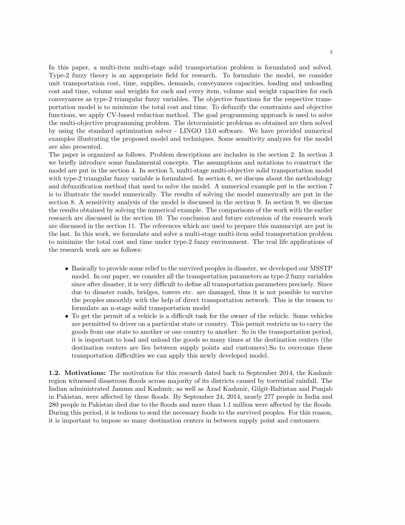
8.2. Sensitivity Analysis of the availabilities and demands of the model. We know thatthe sensitivity analysis is used to analyze the outputs with the given inputs data. For this reason,in Table-5 and -6 we analyze some inputs data and outputs as sensitivity analysis. Basically theminimization of cost objective and time objective in the STP depend on the values of the trans-portation parameters such as unit transportation costs, times, demands, supplies etc.

25

Table-5: Sensitivity analysis on availabilities

αc αt αavail. αdemand αcon.cap. αweight αvolume Opt. cost Opt. time Item-1 Item-20.10 3574.57 101.08 35.93 27.780.12 3584.04 100.11 35.99 27.84

0.11 0.15 0.16 0.17 0.20 0.22 0.25 3584.13 91.03 36.00 27.850.19 3587.07 99.96 36.02 27.870.25 3601.32 109.94 36.06 27.920.26 5541.09 201.52 40.27 39.020.29 5600.76 189.59 40.27 39.02

0.26 0.29 0.32 0.32 0.35 0.38 0.40 5556.28 211.09 40.27 39.020.35 5544.85 197.75 40.27 39.020.38 5508.48 163.44 40.27 39.020.53 4821.18 216.28 39.85 30.450.58 4811.73 180.94 40.24 30.56

0.52 0.56 0.63 0.60 0.64 0.68 0.72 4857.09 185.68 40.85 30.720.68 4905.02 195.65 40.46 30.910.73 4938.51 179.64 41.72 31.070.77 6093.96 256.79 45.73 32.460.83 6139.95 259.16 46.11 32.56

0.77 0.83 0.87 0.87 0.91 0.95 0.99 6148.66 277.31 46.49 32.660.92 6173.94 280.47 46.83 32.950.98 6187.11 280.50 46.93 33.04

Table-6: Sensitivity analysis on demands

αc αt αavail. αdemand αcon.cap. αweight αvolume Opt. cost Opt. time Item-1 Item-20.13 3539.57 101.08 35.68 27.540.16 3565.36 100.18 35.87 27.71

0.11 0.15 0.17 0.19 0.19 0.22 0.25 3594.08 102.09 36.06 27.920.22 3626.59 101.59 36.27 28.180.25 3664.37 100.28 36.50 28.500.26 4534.36 184.54 37 29.690.29 4962.18 151.40 38.6 33.82

0.26 0.29 0.32 0.32 0.35 0.38 0.40 5563.87 186.38 40.27 39.020.35 6193.2 201.54 42.01 45.830.38 7072.83 199.66 43.83 55.230.53 4751.82 157.77 38.54 30.120.58 4798.8 164.77 39.47 30.35

0.52 0.56 0.60 0.63 0.64 0.68 0.72 4833.92 195.21 40.44 30.610.68 4913.07 200.54 41.47 30.920.73 5013.48 184.95 42.55 31.320.77 5921.35 255.83 43.5 31.710.83 6049.3 273.49 44.89 32.22

0.77 0.83 0.87 0.87 0.91 0.95 0.99 6213.72 234.95 45.74 32.460.92 6237.77 266.98 46.67 32.690.98 6271.87 233.34 47.69 32.93

26

8.3. Pictorial representation of the sensitivity analysis. The Pictorial representation of thesensitivity analysis are shown in the figure-2 - figure-17 and those are given below:

Figure 2. Change of total optimum cost and time with Credibility level of avail-ability, αavail. ∈ (0, 0.25]

Figure 3. Change of total optimum cost and time with Credibility level of avail-ability αavail. ∈ (0.25, 0.50]

27

Figure 4. Change of total optimum cost and time with Credibility level of avail-ability, αavail. ∈ (0.50, 0.75]

Figure 5. Change of total optimum cost and time with Credibility level of avail-ability, αavail. ∈ (0.t5, 1]

28

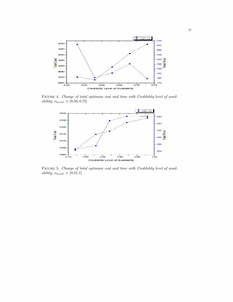
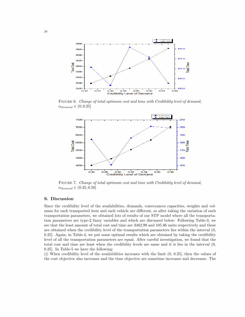
Figure 6. Change of total optimum cost and time with Credibility level of demand,αdemand ∈ (0, 0.25]

Figure 7. Change of total optimum cost and time with Credibility level of demand,αdemand ∈ (0.25, 0.50]

9. Discussion

Since the credibility level of the availabilities, demands, conveyances capacities, weights and vol-umes for each transported item and each vehicle are different, so after taking the variation of eachtransportation parameters, we obtained lots of results of our STP model where all the transporta-tion parameters are type-2 fuzzy variables and which are discussed below: Following Table-3, wesee that the least amount of total cost and time are 3482.99 and 105.86 units respectively and theseare obtained when the credibility level of the transportation parameters lies within the interval (0,0.25]. Again, in Table-4, we put some optimal results which are obtained by taking the credibilitylevel of all the transportation parameters are equal. After careful investigation, we found that thetotal cost and time are least when the credibility levels are same and it is lies in the interval (0,0.25]. In Table-5 we have the following:(i) When credibility level of the availabilities increases with the limit (0, 0.25], then the values ofthe cost objective also increases and the time objective are sometime increases and decreases. The

29

Figure 8. Change of total optimum cost and time with Credibility level of demand,αdemand ∈ (0.50, 0.75]

Figure 9. Change of total optimum cost and time with Credibility level of demand,αdemand ∈ (0.75, 1]

increase or decrease of the total time within the variation of the credibility level is also significanti.e., if we change the credibility level then the allocations are changed and for this reason, it ishappening.(ii) From the third row of the Table-5, we obtained some optimal results of the objectives wherethe credibility level of availabilities are lies within (0.25, 0.5]. Due to change of credibility level ofavailabilities, sometimes the value of total cost are increased and sometimes decreased but thereis no significant change in time objective. This is found when credibility level increases within therange (0.25, 0.5].(iii) The value of the cost objective increases when we increase the credibility level of availabilitieswithin the range (0.5, 0.75] but there are some random changes found in the time objective function.(iv) When credibility level of the availabilities increases within the limit (0.75, 1], then the value ofthe objectives and transported amounts (item-1 and item-2) are increased.Again if we can change the value of the credibility level of the demand, then we found some signif-icant changes on the objective functions as well as transported amounts. From Table-6, it is seen

30

Figure 10. Change of transported amounts (item-1 and 2) with Credibility levelof demand, αdemand ∈ (0, 0.25]

Figure 11. Change of transported amounts (item-1 and 2) with Credibility levelof demand, αdemand ∈ (0.25, 0.50]

that when we increase the credibility level of the demands, then the cost and time objectives arealso increases and same type of changes is found on the transported amount in the final stages.

10. Comparison with the earlier Research work

Heragu [13] introduced the problem called two stages TP and gave the mathematical model forthis problem. The model includes both the inbound and outbound transportation cost and aims tominimize the overall cost. Hindi et al. [12] addressed a two-stage distribution-planning problem.They considered two additional requirements on their problem. First, each customer must be servedfrom a single DC. Second, it must be possible to ascertain the plant origin of each product quantitydelivered. A mathematical formulation called PLANWAR presented by Pirkul and Jayaraman [20]to locate a number of sources and destination centers and to design distribution network so thatthe total operating cost can be minimized. Syarif and Gen [23] considered production/distributionproblem formulated as two-stage TP and proposed a hybrid genetic algorithm (GA) for solution.

31

Figure 12. Change of transported amounts (item-1 and 2) with Credibility levelof demand, αdemand ∈ (0.50, 0.75]

Figure 13. Change of transported amounts (item-1 and 2) with Credibility levelof demand, αdemand ∈ (0.75, 1]

But in our research, we develop a new concept which is totally different from the concept of [20],[13], [12], [23] etc. Here our concept is to supply the commodities from sources to destination centerswith their requirements in stage-1 and then the transported amounts in stage-1 is converted to theavailabilities of the stage-2. The transportation of the stage-2 happened according to requirementsof the destination centers of the stage-2 where the availabilities for the stage-2 are the transportedamounts for stage-1 and so on for the other stage transportations. So we can’t make comparison ofour approach to the existing one. But we validate our technique and optimum result by sensitivityanalysis.

11. Conclusion and Future Extension of the Research Work

11.1. Conclusion. In this paper, we propose a newly developed STP model under type-2 fuzzyenvironment. Weight and volume of the transported items and vehicle are more significant in the

32

Figure 14. Change of transported amounts (item-1 and 2) with Credibility levelof demand, αavail. ∈ (0, 0.25]

Figure 15. Change of transported amounts (item-1 and 2) with Credibility levelof demand, αavail. ∈ (0.25, 0.50]

transportation network. So we add two new additional constraints as weight constraints and volumeconstraints for each vehicle to handle the STP with different stages. We apply the goal program-ming method is to solve our multi-objective multi-stage STP since goal programming techniquegives the better optimal result of the objective function than the other methods. Here we studyfour cases of the credibility level of the different transportation parameters. Also, after solving thetransportation model, we see that the least transportation cost is obtained when the credibilitylevel lies within the range (0, 0.25] and in particular when the credibility level of the transportationparameters are all equal, then a similar type of change is observed in the objective functions. Weobtain the optimal solution of the model by using generalized reduced gradient technique (LINGO13.0 optimization solver) and the results are very effective in real-life sense. So we conclude that,if the credibility levels of the transportation parameters lies within (0, 0.25], then any multi-stageor single stage STP with type-2 fuzzy parameter gives the least value of the objective function.

33

Figure 16. Change of transported amounts (item-1 and 2) with Credibility levelof demand, αavail. ∈ (0.50, 0.75]

Figure 17. Change of transported amounts (item-1 and 2) with Credibility levelof demand, αavail. ∈ (0.75, 1]

11.2. Future Extension of the Research Work. The future extensions of our research workare as follows:• We have formulated the STP model under type-2 fuzzy environment but this model can be de-veloped under fuzzy-rough, fuzzy-random, interval type-2 fuzzy environments etc.• In our model we imposed two extra restrictions with the help of weights and volume of each itemsand vehicles. There is a scope to formulate and solve the model with safety constraints, budgetconstraint etc.• In the objective function we considered the unit transportation cost, time, purchasing cost, load-ing and unloading cost and time etc. but there is a scope to develop the cost objective function ofour model with fixed charges, vehicle carrying cost etc.• In the solution of the imprecise STP model, the transported amounts have been considered ascrisp. Hence there is a scope of taking these transported amount as fuzzy also i.e. the models canbe formulated as fully fuzzy models.

34

References

[1] Qin, R., Liu, Y. K. and Liu, Z. Q. ”Methods of critical value reduction for type-2 fuzzy variables and theirApplications”, Journal of Computational and Applied Mathematics, 235, 1454-1481 (2011).

[2] Karnik, N.N., and Mendel, J.M.,”Centroid of a type-2 fuzzy set”, Information Sciences, 132, 195-220 (2001).

[3] Liu, F.,”An efficient centroid type-reduction strategy for general type-2 fuzzy logic system”, Information Sciences,178, 2224-2236(2008).

[4] Qiu, Y., Yang, H., Zhang, Y.-Q. and Zhao, Y.,”Polynomial regression interval-valued fuzzy systems”, Soft Com-

puting, 12, 137-145 (2008).[5] Haley, K.B.,”The solid transportation problem”, Operations Research,10, 448-463(1962).

[6] Haley, K.B.,”The multi-index problem”, Operations Research,11,368-379(1963).

[7] Hitchcock, F.L.,”The distribution of a product from several sources to numerous localities”, Journal of Mathe-maticalPhysics, 20,224-230(1941).

[8] Shell, E.,”Distribution of a product by several properties, in: Directorate of Management Analysis”, Proceedings

of the Second Symposium in Linear Programming”, 2, 615-642, DCS/Comptroller H.Q.U.S.A.F., Washington,DC. (1955).

[9] Zadeh, L.A.,”Concept of a linguistic variable and its application to approximate reasoning I”, Information Sci-

ences, 8, 199-249 (1975).[10] Mitchell, H.,”Ranking type-2 fuzzy numbers”, IEEE Transactions on Fuzzy Systems, 14, 327-348 (2006).

[11] Liang, Q. and Mendel, J.M.,”Interval type-2 fuzzy logic systems: theory and design”, IEEE Transactions onFuzzy Systems, 8, 535-549 (2000).

[12] Charnes, A., Cooper, W.W. and Rhodes, E. ”Measuring the efficiency of decision making units”, European

Journal of Operational Research, 6, 429-444 (1978).[13] Sengupta, J.K.,”Efficiency measurement in stochastic input-output systems”, International Journal of System

Science, 13, 273-287 (1982).

[14] Banker, R.D.,”Maximum likelihood, consistency and DEA: statistical foundations”, Management Science, 39,1265-1273 (1993).

[15] Cooper, W.W., Huang, Z.M., Li, S.X. and Olesen, O.B., ”Chance constrained programming formulations for

stochastic characterizations of efficiency and dominance in DEA”, Journal of Productivity Analysis, 9, 53-79(1998).

[16] Land, K.C., Lovell, C.A.K. and Thore, S.,”Chance constrained data envelopment analysis”, Managerial and

Decision Economics, 14, 541-554 (1993).[17] Heragu S., ”Facilities design”, PWS (1997).

[18] Baidya, A., Bera, U. K. and Maiti, M., ”Solution of multi-item interval valued solid transportation problemwith safety measure using different methods”, OPSEARCH, 51(1), 1-22 (2013).

[19] Geoffrion A. M. and Graves G. W., ”Multi commodity distribution system design by benders decomposition”,

Manage Sci, 20, 822-844 (1974).[20] Pirkul H, Jayaraman V. ”A multi-commodity, multi-plant capacitated facility location problem: formulation

and efficient heuristic solution”, Computer and Operations Research, vol. 25 (10), pp. 869-878(1998).

[21] Hindi K. S., Basta T. and Pienkosz K., ”Efficient solution of a multi-commodity, two-stage distribution problemwith constraints on assignment of customers to distribution centers”, Int Trans Oper Res vol. 5(6), pp. 519-

527(1998).

[22] Syarif A. and Gen M. ”Double spanning tree-based genetic algorithm for two stage transportation problem”,Int J Knowl-Based Intell Eng Syst, 7(4) (2003).

[23] Ali Amiri, ”Designing a distribution network in a supply chain system: formulation and efficient solutionprocedure” Eur J Oper Res, vol. 171, pp. 567-576(2006).

[24] Gen, M., Altiparmak, F. and Lin, L., ”A genetic algorithm for two-stage transportation problem using priority-

based encoding”, OR Spectrum, Vol. 28, pp. 337-354 (2006).[25] Mahapatra, G. S. and Roy, T. K., ”Fuzzy multi-objective mathematical programming on reliability optimization

model”, Applied Mathematics and Computation, vol. 174, pp. 643-659(2006).

[26] Kundu, P., kar, S. and Maiti, M., ”Fixed charge transportation problem with type-2 fuzzy variable”, InformationSciences, vol. 255, pp. 170-186 (2014).

[27] Yang, L. and Feng, Y., ”A bicriteria solid transportation problem with fixed charges under stochastic environ-

ment”, Applied Mathematical Modelling, vol.31, pp. 2668-2683 (2007).[28] Kundu, P., kar, S. and Maiti, M., ”Multi-objective multi-item solid transportation problem in fuzzy environ-

ment”, Applied Mathematical Modelling, vol. 37, pp. 2028-2038 (2012).

35

[29] Liu, P., Yang, L., Wang, L. and Liu, S., ”A solid transportation problem with type-2 fuzzy variables”, AppliedSoft Computing, vol. 24, pp. 543-558 (2014).

[30] Yang, L., Liu, P., Li, S., Gao, Y. and Ralescu, D.A., ”Reduction method of type-2 uncertain variables and their

applications to solid transportation problems”, Information Sciences, vol. 291, pp. 204-237 (2015).[31] Giri, P. K., Maiti, M. K. and Maiti, M., ”Fully fuzzy fixed charge multi-item solid transportation problem”,

Applied Soft Computing, vol. 27, pp77-91 (2015).[32] Yang, L. and Liu, L., ”Fuzzy fixed charge solid transportation problem and algorithm”, Applied Soft Computing,

vol. 7, pp. 879-889 (2007).

[33] Molla-Alizadeh-Zavardehi, S., Sadi Nazhad, S., Tavakkoli-Moghaddam, R. and Yazdani, M., ”solving a fuzzyfixed charge solid transportation problem and by metaheuristics”, Mathematical and Computer Modelling, vol.

57, pp. 1543-1558 (2013).