Multi-Structural Databases

Ronald Fagin R. Guha Ravi Kumar

Jasmine Novak D. Sivakumar Andrew Tomkins

IBM Almaden Research Center650 Harry Road

San Jose, CA 95120nfagin, guha, ravi, jnovak, siva, tomkins

o@almaden.ibm.com

ABSTRACTWe introduce the Multi-Structural Database, a new dataframework to support efficient analysis of large, complexdata sets. An instance of the model consists of a set of dataobjects, together with a schema that specifies segmentationsof the set of data objects according to multiple distinct crite-ria (e.g., into a taxonomy based on a hierarchical attribute).Within this model, we develop a rich set of analytical opera-tions and design highly efficient algorithms for these opera-tions. Our operations are formulated as optimization prob-lems, and allow the user to analyze the underlying data interms of the allowed segmentations.

1. INTRODUCTIONConsider a large collection of media articles that could be

segmented by a number of “dimensions.”◦ By time: articles from April 2004, or from 1978;◦ By content type: articles from newspapers, or from

magazines, and within magazines, from business magazines,or from entertainment magazines;◦ By geography: articles from the U.S., or from Europe,

and within Europe, from France or from Germany;◦ By topic: articles about a war, a hurricane, or an elec-

tion, and within these topics, by subtopic.These different dimensions may be correlated; for instance,

knowing the content type may give information about thetopics. The first dimension in this list (time) can be viewedas numerical and as the example shows, we may be inter-ested in intervals of time at various granularities. The otherthree dimensions in this list (content type, geography, andtopic) can be viewed as hierarchical.

Because of the rich nature of the data (in this case, doc-uments), we would be interested in probing the data withqueries that are much richer than those in a typical databasesystem. For example, we might be interested in the followingtypes of queries.

Permission to make digital or hard copies of all or part of this work forpersonal or classroom use is granted without fee provided that copies arenot made or distributed for profit or commercial advantage and that copiesbear this notice and the full citation on the first page. To copy otherwise, torepublish, to post on servers or to redistribute to lists, requires prior specificpermission and/or a fee.PODSJune 13–15, 2005, Baltimore, MD.Copyright 2005 ACM 1-59593-060-4/05/06 ...$5.00.

◦ What are the ten most common topics in the collection?◦ From 1990 to 1995, how did articles break down across

geography and content type?◦ Which subtopics caused the sudden increase in dis-

cussion of the war? Are these subtopics different amongEuropean newspapers?◦ Break the early 1990s into ten subperiods that are most

topically cohesive, and explain which topics were hot duringeach period.◦ Break documents that mention the President by topic

so that they are most closely aligned with different contenttypes, to capture how different types of media with differentaudiences focused on particular topics.

One of the first things we notice about these queries isthat they are rather fuzzy: there is not necessarily a clear“right answer.” Even after we supply certain parameters (aswe will do later), there may not be a unique answer. Thereis another way that our queries are unlike standard databasequeries. Our queries will be resolved not by, say, searchingindices, but instead by an optimization procedure.1 Mostimportantly, these queries seek to provide the user with thehighlights or salient characteristics of the data set.

Our main contribution is a framework for expressing andcomputing the highlights of a large and complex data set.This includes a data model that is rich enough to representthe kinds of structures found in real applications. Withinthis model, we propose Pairwise Disjoint Collections (orPDCs, to be defined shortly) as a basic notion that capturesthe intuitive idea of a concise set of highlights of a dataset. We formulate rich queries as optimization problemsthat map the underlying data into a succinct PDC withinthe allowed “schema.” Finally, we provide efficient algo-rithms that give approximately optimal solutions for threeimportant classes of objective functions. We illustrate theuse of our framework with experimental results.

The basic framework.We define a multi-structural database (MSDB) to consist

of a schema (the set of dimensions, which, in our example,are time, content type, geography, and topic), and a set of

1Optimization procedures arise also in relational databasesystems, such as in trying to find the most efficient way toevaluate an SQL query. However, the answer to the SQLquery is independent of the result of the optimization. Incontrast, for our queries, the answer to the query is actuallythe result of the optimization procedure.

objects (the data, which, in our example, are media arti-cles).

The intent of the schema is to specify how the set of dataobjects may be segmented based on each dimension. Noticethat each type of dimension admits partitions in a naturalway, e.g., a numerical dimension may be partitioned intointervals, and a hierarchical dimension into collections oftaxonomy nodes. Our first technical contribution is a uni-fied approach to handling these diverse types. Namely, weformalize each dimension as a lattice — e.g., the geographydimension is a lattice whose elements include Europe andFrance, and the time dimension is a lattice whose elementsare intervals at various granularities.

As usual, a lattice is endowed with meet and join (seeSection 3 for definitions). For example, in the geographydimension, the join of the European countries is Europe,and in the time dimension, the meet of two time intervals istheir intersection. Each data element (in our example, eachdocument) is associated with various elements in the lattice.When a data item is associated with a lattice element, it isalso associated with every element above it in the lattice;for example, a document about France is also a documentabout Europe. Lattice elements whose meet is bottom, theminimal element of a lattice, are thought of as disjoint con-cepts. For example, in the topics dimension, Sports andPolitics are thought of as disjoint concepts. However, it isimportant to note that there may be a document associatedwith both of these concepts (such as a document about abodybuilder who is also a governor).

We shall also consider new lattices that are the result oftaking the product of a subset of our lattices. For example,“French newspaper” is an element of the lattice that is theproduct of the geography lattice and the content type lattice.

Besides unifying various types of allowed segmentations ofdata, our lattice-based approach offers the additional benefitof being able to concisely describe subcollections of the data.Elements of a lattice are restrictions like “French newspa-per,” and hence can be easily understood by a user in theterms used to define the schema. Indeed, the fundamentalcollection of data objects in our framework is the set of dataobjects associated with a lattice element.

The next key notion in our framework is that of a pair-wise disjoint collection (PDC). This is a set of elements of alattice whose pairwise meet is bottom. A PDC thus repre-sents a collection of conceptually disjoint concepts, and willbe our model of what a data analysis operation returns tothe user.

Analytical operations and algorithms.Analogous to the way we developed an enhanced data

model to support data analysis, we also enhance the no-tion of what constitutes a “query.” As mentioned earlier,our analytical operations will be formulated as optimizationproblems that map the set of data objects into a PDC withinthe schema. In the present paper, we develop the formalismand algorithms for three main query families, each of whichsupports a fairly general data analysis operation. We be-lieve that our model is fairly powerful, and anticipate manymore rich queries to be developed within our framework.

The Divide operation seeks to determine how a set ofobjects is distributed across a particular set of dimensions.The goal of the Divide operation is to return a small PDCin which the documents are divided as evenly as possibleamong the elements of the PDC with respect to the set of

dimensions; thus, Divide provides a concise summary of thedata. For example, a Divide operation with respect to geog-raphy, where the goal is to partition into ten approximatelyequal-sized pieces, might show that 11% of documents comefrom North America, 9% come from Western Europe, andso on.

The Differentiate operator allows the user to comparetwo different document sets with respect to certain dimen-sions. For example, a user could observe that there aremany more blog entries in July than the rest of the year,and could employ Differentiate to determine how muchparticular topics or geographies explain the spike. Thus, theDifferentiate operation helps us to find surprises in thedata.

The goal of the Discover operation is to break up a doc-ument set so that an internal pattern becomes visible. Theoperation segments the data using one set of dimensions suchthat the resulting segments are cohesive and well-separatedaccording to another set of dimensions. For example, a usermight ask if there is a way to break up newspaper articles bytopic so that a strong geographic bias emerges. Thus, theDiscover operation helps us to find interesting “regions”and structure in the data.

While our lattice-based formulation is quite general, forthe sake of obtaining efficient algorithms, we focus on twospecial cases of dimensions: numerical and hierarchical. Thesetwo special cases arise frequently in practice and hence it isimportant to develop efficient algorithms for these. We firstshow that in general it is NP-hard to approximate any of ouranalytic operations. On the other hand, we obtain exact al-gorithms for the single-dimensional case and approximationalgorithms for the multi-dimensional case. Most of our al-gorithms are based on dynamic programming and can beimplemented very efficiently.

We have implemented these operations in a prototype sys-tem, and created three databases within this system. Thefirst database consists of pages from the World Wide Web;the second contains information about books and their salesranks at amazon.com over time; and the third contains med-ical articles from medline. In all cases, a set of appropriatehierarchical and numerical dimensions are defined. We givea set of representative results showing that the operationsare both natural and useful on real-world data.

2. RELATED WORK

2.1 Online Analytical ProcessingOur formulation maps directly to those that have been

used in OLAP [4]. A traditional formulation (for example,that of Kimball [19], or see [28] for a survey) distinguishesbetween measures, which are numerical and are the targetof aggregations, and dimensions, which are often hierarchi-cal. However, this distinction is not required, and there areformulations in which both are treated uniformly, as in oursystem. See Agrawal et al. [1], and Gyssens and Laksh-manan [14], for such examples.

Further, Harinarayan et al. [16] describe a formulationin which each dimension is a lattice, and a joint latticeis defined over multiple dimensions; this formulation ex-actly matches our model, except that our goal is to performoptimizations over the resulting multi-dimensional lattice,rather than to characterize the set of possible queries andhence the candidate materializations.

Gray et al. [10] describe, in the context of the cube oper-ator, aggregation functions that may be distributive, alge-braic, or holistic. Our algorithms rely on similar propertiesof the scoring functions we employ to determine the qualityof a particular candidate solution to our optimization prob-lems. We consider both distributive and algebraic scoringfunctions.

Cody et al [5] consider the “BIKM” problem of unifyingbusiness intelligence and knowledge management, by cre-ating data cubes that have been augmented by additionalinformation extracted through text analysis. They use anOLAP model similar to ours in that the granularity of thefact table is a single document.

Much work on OLAP considers materialization of partic-ular views in order to improve query performance. Thesequestions are relevant in our setting, but we do not considerthem in this work.

Cabibbo and Torlone [3] propose that OLAP systems shouldsupport multiple query frameworks, possibly at differentlevels of granularity. There have been a number of suchapproaches suggesting frameworks that move beyond tradi-tional hypothesis-driven query models into discovery-drivenmodels. Han [15] and others have considered data miningto extract association rules on cubes. Sarawagi et al. [24,25, 26] identify areas of the data space that are likely tobe surprising to the user. Their mechanisms allow the userto navigate the product lattice augmented with indicatorssuggesting which cells at a particular location are surpris-ing, and which paths will lead to surprising cells. Theirvisualization applies to our techniques, and their notion of“surprisingness” may be viewed as an operator to which ourtechniques apply. Like us, they produce exceptions at alllevels of the cube, rather than simply at the leaves.

Lakshmanan et al. [20] consider partitions of the cube inorder to summarize the “semantics” of the cube; all elementsof a partition belong to the same element of a particular typeof equivalence relation. This partitioning is similar in spiritto our notion of a complete PDC.

A few properties of our model that (are not necessarily dis-tinguishing, but nevertheless) should be kept in mind whencomparing to traditional OLAP systems include the follow-ing. Typically, an OLAP fact table contains a single entryfor each cell of the cube; this is typically not the case inour setting, or in that of [5]. Also, our objects may belongto multiple locations within a dimension, which is typicallynot the case in OLAP (with certain lattices correspondingto time as notable exceptions). Our dimensions are typicallynot required to be leveled or fixed-depth. And we often con-sider single dimensions in which the size of the lattice isquadratic in the number of distinct leaves (all intervals of aline, for example).

Additionally, there is a fundamental distinction betweenour work and OLAP, which relates to the nature of queriesrather than to the data model. OLAP queries typically spec-ify certain nodes of the multi-dimensional lattice for whichresults should be computed; these nodes might be all themonths of 2003 crossed with all the products in a certaincategory, for example. Our goal instead is to leave the choiceof nodes to return as a constrained set of choices availableto the algorithm, and to cast the problem of selecting a setof nodes as an optimization.

2.2 Clustering and miningSome of our operations, especially Discover, can be viewed

as solving classification or clustering problems. While thereis a vast literature on clustering involving numerical at-tributes, only recently has the problem of clustering involv-ing a combination of numerical and categorical attributesgained much attention. Systems such as ROCK [13], CAC-TUS [8] and COOLCAT [2] provide algorithms for clusteringdata described by a combination of numerical and categor-ical attributes. In contrast to these, which assume a flatspace of categorical attributes, MSDB goes one step fur-ther in using a lattice structure of relationships between thedifferent values for each dimension. The addition of thisstructure allows us to restrict the clusters identified to cor-respond to nodes that are already in the lattice, which makethe clusters easier for the user to understand.

Additionally, our goal of finding useful patterns in a dataset is similar to the goals of data mining. While much ofthe attention in data mining has been on inducing associ-ation rules, the work reported in [7, 9, 21] has consideredthe problem of trend discovery and analysis. We continuetowards this goal by enriching the underlying data modeland generalizing the notion of a trend.

Finally, the algorithmic questions that arise in certain ofour optimization problems are related to various questionsthat have been studied; we give pointers to this literature inthe context of the algorithms themselves.

3. FORMULATIONSA lattice is a representation of a partial ordering on a

set of elements. It may be defined in terms of a partialorder, or in terms of the operations meet, written ∧, andjoin, written ∨. We give the latter definition since we willuse this formulation more heavily. A lattice then is a set ofelements closed under the associative, commutative binaryoperations meet and join, such that for all elements a andb, we have a ∧ (a ∨ b) = a ∨ (a ∧ b) = a. The lattice inducesa natural partial order: a ≤ b if and only if a∧ b = a. For alattice L, we will write a ∈ L to mean that a is an elementof the set.

A lattice is bounded if it contains two elements > and ⊥,called top and bottom, such that a ∧ ⊥ = ⊥ and a ∨ > = >for all elements a. All finite lattices are bounded.

We will use #(A) to refer to the cardinality of set A.

3.1 MSDBA multi-structural database (or simply MSDB) (X, D, R)

consists of a universe X = {x1, . . . , xn} of objects, a setD = {D1, . . . , Dm} of dimensions, and a membership rela-tion R specifying the elements of each dimension to whicha document belongs. We will treat each xi as simply anidentifier, with the understanding that this identifier mayreference arbitrary additional data or metadata. In the fol-lowing, we will often refer to objects as documents, as thisis a key application domain. A dimension Di is a boundedlattice, and we assume that the lattice nodes used in all lat-tices are distinct; the vocabulary V = ∪iDi consists of allsuch lattice nodes. The membership relation R ⊆ X × Vindicates that a data object “belongs to” a lattice element.We require that R be upward closed, i.e., if 〈x, `〉 ∈ R and` ≤ `′, then 〈x, `′〉 ∈ R. We define X|`, read X restricted to`, as X|` = {x ∈ X | 〈x, `〉 ∈ R}.

Similarly, we can define multiple dimensions to have thesame structure as single dimensions. For nonempty D′ ⊆ D,the multi-dimension MD(D′) is defined as follows. If D′ isa singleton, the multi-dimension is simply the dimension ofthe single element. Otherwise, if D′ = {D1, . . . , Dd}, thenMD(D′) is again a lattice whose elements are {〈`1, . . . , `d〉 |`i ∈ Li}, where 〈`11, . . . , `1d〉∨〈`21, . . . , `2d〉 = 〈`11 ∨ `21, . . . , `

1d ∨ `2d〉,

and likewise for ∧. The membership relation R is then ex-tended to contain 〈x, 〈`1, . . . , `d〉〉 if and only if it contains〈x, `i〉 for all i. This lattice is sometimes called the directproduct of the dimensional lattices [27].

Interpretation of lattice elements.We think of each lattice element as a conceptual way of

grouping together documents. All elements of the same lat-tice should represent conceptual groupings within the samelogical family, for example, groupings of documents based ontheir topic. The meet of two conceptual groupings shouldbe seen as the most general concept that is a specializationof both. For example, the meet of documents referring toevents of the 1800s and documents referring to events from1870-1930 should be documents referring to events from1870-1899. Likewise, the join of two conceptual groupingsshould be seen as the most specific concept that is a gen-eralization of both. The join of the two concepts describedabove should be all documents referring to events occurringbetween 1800 and 1930. Two concepts whose meet is ⊥should be seen as conceptually non-overlapping. It is pos-sible that objects in the database could be part of bothgroups. For example, a dimension capturing a particularway of breaking documents into topics might contain a sub-tree about Sports, with a subnode about Basketball; andmight also contain elsewhere a node about Politics. Justbecause a document appears that happens to discuss bothSports and Politics (because it is about sports legislation),this does not mean that the two topics must be conflatedin the formalism. The membership relation allows a docu-ment to belong to two lattice elements whose meet is ⊥. Astrength of our formalism is that dimensions represent ab-stract conceptual groupings, but individual objects need notadhere exactly to these groupings. Of course, as individualdocuments belong to more and more conceptually disjointregions of a dimension, the discriminative power of that di-mension will diminish.

3.2 Pairwise disjoint collectionsWe now introduce our key notion, which will be used

in the definition of all three analytical operations. Intu-itively, a pairwise disjoint collection, abbreviated PDC, is away of breaking a set of documents into conceptually non-overlapping pieces such that each piece can be easily de-scribed using the elements of a particular multi-dimension.Formally, for any multi-dimension MD(D′) and any set S ={`1, . . . , `d} of elements of the multi-dimension, we say thatS is a PDC if `i ∧ `j = ⊥ for all i, j with i 6= j.

So a PDC, in contrast to a general set of clusters, canbe communicated easily and concisely to the user in termsthat already exist in the schema; namely, the particular el-ements of MD(D′) that define each PDC member. Eachof our analytical operations takes a multi-dimension, andother information, and returns a PDC over the given multi-dimension, using the other information to determine whichPDC should be returned.

In general, we think of a PDC as a segmentation of the

conceptual space of the database. For example, a PDCmight contain both the Sports and Politics nodes of a di-mension capturing topic, as these nodes meet at ⊥ — theydo not share any subconcepts. Of course, as discussed above,there may be a document that exists in both nodes at oncebecause it discusses Sports Legislation.

As another example, consider two numerical dimensions,and the associated multi-dimension. A PDC in this multi-dimension corresponds to a tiling of the plane using axis-parallel rectangles.

We say a PDC is complete for a subset X ′ ⊆ X of theobjects if for every x ∈ X ′, there is some ` in the PDC suchthat 〈x, `〉 ∈ R; that is, every document belongs to someelement of the PDC. We say that a PDC is complete tomean that it is complete for X.

The reader might ask why the dimensions of an MSDB arenot simply formulated as a set system of documents with in-tersection and union, rather than a lattice; in this case, aPDC would be a collection of mutually non-overlapping setsof documents. This notion of PDC is problematic becauseas we discussed, documents in practice may belong to mul-tiple conceptually distinct categories. We circumvent thisproblem by defining PDCs at the schema level, rather thanthe instance level.

Restricted classes of PDCs.In many situations, conveying to the user an arbitrary

PDC over a complex multi-dimension may be quite difficult,and we may choose to restrict the allowable PDCs. Like-wise, in some situations, optimal instances of a restrictedfamily of PDCs may be easier to compute than for gen-eral PDCs. We define three types of increasingly restrictivePDCs. First, we require a definition. Consider a PDC Hover MD(D′), and assume dimension Di ∈ D′. Let H|Di ={`i | 〈`1, . . . , `d〉 ∈ H} and for any element ` ∈ H|Di ,let H|Di

(`) = {〈`1, . . . , `i−1, `i+1, . . . , `d〉 | 〈`1, . . . , `d〉 ∈H, `i = `}.

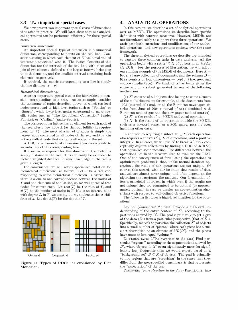
General: A general PDC has no restrictions.

Sequential: Intuitively, a sequential PDC first breaks thedata via a PDC in some dimension, then recursively subdi-vides each resulting data set using the next dimension, andso on. In our earlier example of two numerical dimensions,a PDC that is sequential will contain either horizontal orvertical strips, each of which may be broken respectively byarbitrary vertical or horizontal lines. Formally, a sequentialPDC is defined recursively as follows.

A PDC over a single dimension is sequential.A PDC H over D′ ⊆ D is sequential for an ordering

(D′1, . . . , D

′d) of the dimensions D′ if H|D′

dis a PDC and

H|D′

d(`) is sequential for (D′

1, . . . , D′d−1) for all ` ∈ H|D′

d.

A PDC is sequential for D′ if there exists an ordering ofD′ for which it is sequential.

Factored: Intuitively, a PDC is factored if it represents thecross-product of PDCs in each dimension. In our exampleof two numerical dimensions, a factored PDC is defined by aset of vertical and horizontal lines. Formally, a PDC H overD′ ⊆ D is factored if H = H|D1 × · · · × H|D#(D′) . Every

factored PDC is a sequential PDC for every ordering of thedimensions.

A graphical representation of examples of the three typesof PDCs for two numerical dimensions is shown in Figure 1.

3.3 Two important special casesWe now present two important special cases of dimensions

that arise in practice. We will later show that our analyti-cal operations can be performed efficiently for these specialcases.

Numerical dimensions.An important special type of dimension is a numerical

dimension, corresponding to points on the real line. Con-sider a setting in which each element of X has a real-valuedtimestamp associated with it. The lattice elements of thisdimension are the intervals of the real line, with meet andjoin of two elements defined as the largest interval belongingto both elements, and the smallest interval containing bothelements, respectively.

If required, the metric corresponding to a line is simplythe line distance |x− y|.

Hierarchical dimensions.Another important special case is the hierarchical dimen-

sion, corresponding to a tree. As an example, considerthe taxonomy of topics described above, in which top-levelnodes correspond to high-level topics such as “Politics” or“Sports”, while lower-level nodes correspond to more spe-cific topics such as “The Republican Convention” (underPolitics), or “Curling” (under Sports).

The corresponding lattice has an element for each node ofthe tree, plus a new node ⊥ (as the root fulfills the require-ment for >). The meet of a set of of nodes is simply thelargest node contained in all nodes of the set, and the joinis the smallest node that contains all nodes in the set.

A PDC of a hierarchical dimension then corresponds toan antichain of the corresponding tree.

If a metric is required for this dimension, the metric issimply distance in the tree. This can easily be extended toinclude weighted distance, in which each edge of the tree isgiven a length.

For convenience, we will adopt specialized notation forhierarchical dimensions, as follows. Let T be a tree cor-responding to some hierarchical dimension. Observe thatthere is a one-to-one correspondence between the nodes ofT and the elements of the lattice, so we will speak of treenodes for convenience. Let root(T ) be the root of T , and#(T ) be the number of nodes in T . If a is an internal nodewith degree ∆ in T , we use a1, . . . , a∆ to denote the ∆ chil-dren of a. Let depth(T ) be the depth of T .

General Sequential Factored

Figure 1: Types of PDCs, as envisioned by PietMondrian.

4. ANALYTICAL OPERATIONSIn this section, we describe a set of analytical operations

over an MSDB. The operations we describe have specificdefinitions with concrete measures. However, MSDBs arenot formulated solely to support these three operations. Weanticipate both extensions and modifications of our analyt-ical operations, and new operations entirely, over the sameframework.

The three analytical operations we describe are intendedto capture three common tasks in data analysis. All theoperations begin with a set X ′ ⊆ X of objects in an MSDB(X, D, R). For the purposes of illustration, we will adoptour running example of the MSDB of documents. Here X =Docs, a large collection of documents, and the schema D =Dims consists of four dimensions — topic, time, geo, andsource (media type). We think of X ′ as being either theentire set, or a subset generated by one of the followingmechanisms:

(1) X ′ consists of all objects that belong to some elementof the multi-dimension; for example, all the documents from1995 (interval of time), or all the European newspaper ar-ticles from June of 2004 (interval of time combined withEuropean node of geo and the newspaper node of source);

(2) X ′ is the result of an MSDB analytical operation;(3) X ′ is the result of an operation outside the MSDB,

such as a keyword search or a SQL query, possibly evenincluding other data.

In addition to requiring a subset X ′ ⊆ X, each operationalso requires a subset D′ ⊆ D of dimensions, and a positiveinteger k. In all cases, we will use D′ to break X ′ into k con-ceptually disjoint collections by finding a PDC of MD(D′)that optimizes some measure. The differences between theoperations lies in the measure used to evaluate the PDC.One of the consequences of formulating the operations asoptimization problems is that, unlike normal database op-erations, the result of our operations are not unique. Ofcourse, this accords with our intuition that results of dataanalysis are almost never unique, and often depend on thealgorithm that performs the analysis. Our formulation of-fers a principled approach in which even if the results arenot unique, they are guaranteed to be optimal (or approxi-mately optimal, in case we employ an approximation algo-rithm) with respect to well-defined objective functions.

The following list gives a high-level intuition for the oper-ations:

Divide: (Summarize the data) Provide a high-level un-derstanding of the entire content of X ′, according to thepartitions allowed by D′. The goal is primarily to get a gistof the data (X ′) from a particular perspective (that of D′).Specifically, we seek to partition the collection X ′ of objectsinto a small number of “pieces,” where each piece has a suc-cinct description as an element of MD(D′), and the pieceshave more or less equal “volume.”

Differentiate: (Find surprises in the data) Find par-ticular “regions,” according to the segmentations allowed byD′, where objects in X ′ occur significantly more (or signif-icantly less) frequently than we would expect based on a“background set” B ⊆ X of objects. The goal is primarilyto find regions that are “surprising” in the sense that theydiffer from the user-specified benchmark B that representsthe “expectation” of the user.

Discover: (Find structure in the data) Partition X ′ into

pieces according to the segmentations allowed by D′ suchthat the pieces represent cohesive, well-separated clusterswhen evaluated according to a metric on the lattice of an-other set M ⊆ D of dimensions. The goal is to take the un-differentiated set X ′ of objects and find some way to breakit up according to D′ so that structure emerges, in the sensethat each of the identified regions looks different throughthe lens of the measurement dimensions M .

We now formally define these operations.

4.1 Divide

The Divide operation allows the user to see at a high levelhow a set of objects is distributed across a particular set ofdimensions. In our example MSDB, a Divide operationwith respect to geo, where the goal is to partition into tenapproximately equal-sized pieces, might show that 11% ofmedia documents come from North America, 9% come fromWestern Europe, etc. The goal of the Divide operation isto identify a PDC from a specified set D′ of dimensions thatis complete for X ′. On the one hand, we would like thePDC to be small, that is, to consist of a small number ofelements of MD(D′), so that it may be conveyed to the usersuccinctly (e.g., on a screen); on the other hand, a PDC withten elements, one of which contains 99% of the documentsin X ′, is a poor choice since it does not give the user a goodview of how the objects are spread out along D′. Ideally, wewould prefer a PDC with ten sets, each of which contains10% of the objects in X ′. The Divide operation allows theuser to specify the size of the PDC, and computes the bestPDC of that size.

FormalismDivide(X, D; X ′, D′, k)Input: X ′ ⊆ X; D′ ⊆ D; k ∈ Z+

Output: A PDC H of MD(D′) of size k such that H iscomplete for X ′, and max

h∈H#(X ′|h) is minimal over all such

H.

ExamplesThe Divide operation may be applied in our running ex-

ample of the Docs MSDB in the following ways:

(1) To partition all documents from 2004 into ten roughlyequal-sized collections, where each collection can be labeledby a specific topic, one may perform

Divide(Docs, Dims ; X ′, {topic}, 10),where X ′ = Docs|time=2004.

(2) To partition all documents into ten roughly equal-sizedcollections, where each collection can be labeled by a specificpair of time and geographic region, one may perform

Divide(Docs, Dims ; Docs, D′, 10),where D′ = {time, geo}.

4.2 Differentiate

The Differentiate operation allows the user to comparetwo different sets of objects with respect to certain dimen-sions. This operation is useful when a user has two collec-tions X ′ and B of objects — intuitively, the foreground andbackground collections — that the user knows (or believes)to be different in their distribution across some set D′ of di-mensions, and wishes to find out which regions of MD(D′)best explain the difference between the two collections.

In our (Docs, Dims) example, suppose a user observes thatthere are significantly more blogs in July than in the rest ofthe year; she might seek an explanation in terms of the other

dimensions, namely topic and geo. Similarly, she may seekto explain the difference in the distribution of documentsabout information technology across various source mediatypes from that of documents about management styles.

The Differentiate operation assumes some measure µthat quantifies, for every element h ∈ MD(D′), the differ-ence between X ′|h and B|h; intuitively, µ measures howunlike B the set X ′ is, from the viewpoint of h. For exam-ple, if 2% of all blogs are about art and there are 200K blogentries in July, one would expect about 4K of these blogentries to be about art; if, on the other hand, 13K blogs inJuly are about art, then the excess of 9K is a good indicatorof how unlike the rest of the year July was for blog entriesabout art. With a measure µ in hand, Differentiate seeksto find a small PDC — again, motivated by conciseness ofthe output returned to the user — such that the sum of theµ difference between X ′ and B over all the elements of thePDC is maximized. Thus, in our example, the user mightlearn that art, travel, and baseball form the best set of threetopics that distinguish the July blogs from the rest.

FormalismDifferentiate(X, D; X ′, B, D′, µ, k)Input: X ′ ⊆ X; B ⊆ X; D′ ⊆ D; k ∈ Z+;µ : MD(D′)× 2X × 2X → ROutput: A PDC H of MD(D′) of size k such thatPh∈H

µ(h; X ′, B) is maximal over all such H.

The Measure µWe briefly discuss a suitable choice of the measure func-

tion µ that satisfies certain desirable conditions. Recall thatthe goal of defining µ is that, for a given h ∈ MD(D′) andforeground and background sets X ′ and B, the measure µshould quantify how unlike B|h the set X ′|h is. Specifically,if we treat B as a set of objects that define a “baseline,” for

every set Y of objects, we expect roughly a fraction #(B|h)#(B)

of the objects in Y to be in Y |h; thus, we expect roughly thesame fraction of the objects in X ′ to be in X ′|h. When weare interested in explaining upward surges, a natural candi-date for µ is the excess in #(X ′|h)/#(X ′) over this quantity,namely we define the peak measure µp by

µp(h; X ′, B) = #(X′|h)#(X′) − #(B|h)

#(B).

If we are interested in explaining downward trends, we mayuse the analogous “valley measure,” defined by µv(h; X ′, B) =−µp(h; X ′, B). If we are interested in large upward surgesand downward trends primarily for their magnitude, we mayuse the “absolute measure” µa(h; X ′, B) = |µp(h; X ′, B)|.

Note that the definition of µa simultaneously addressestwo important considerations — how surprising X ′|h is rel-ative to B|h, as well as how impactful X ′|h is. It is obvi-

ous that to achieve a high value of˛#(X′|h)#(X′) − #(B|h)

#(B)

˛, the

fractions should differ substantially, that is, the collectionX ′ should look surprisingly different from B with respectto h; furthermore, since (the absolute value of) this differ-

ence is upper-bounded by max{#(X′|h)#(X′) , #(B|h)

#(B)}, it is easy

to see that µa would only pick elements h for which either#(X ′|h) represents a large fraction of #(X ′) or #(B|h) is alarge fraction of #(B). Similar comments apply to µp andµv as well.Examples

The Differentiate operation may be applied in our run-ning example of the Docs MSDB in the following ways:

(1) To find the top ten geographic regions in which thesport of rugby is covered more heavily than sports in general,one may perform

Differentiate(Docs, Dims ; Xr, Xs, D′, µp, 10),

where Xr = X|topic=Rugby, Xs = X|topic=Sports, and D′ ={geo}.

(2) To find the top three topics whose discussion decreasedsignificantly, going from 2003 to 2004, one may perform

Differentiate(Docs, Dims ; X4, X3, D′, µv, 3),

where X4 = X|time=2004, X3 = X|time=2003, and D′ = {topic}.(3) To find the five best combinations of topics and media

types that occur very differently between Europe and Asia,one may perform

Differentiate(Docs, Dims ; XE , XA, D′, µa, 5),where XE = X|geo=Europe, XA = X|geo=Asia, and D′ ={topic, source}.

(4) Suppose a user notices a spike in the discussion ofwar from July to November of 2002. To find the top tencombinations of media types and geographic regions thataccount for this spike, she may perform

Differentiate(Docs, Dims ; Xw, Xo, D′, µp, 10),

where Xw = X|topic=War,time=[7/2002,11/2002], Xo = X \ Xw,and D′ = {geo, source}.

4.3 Discover

The goal of the Discover operation is to unearth collec-tions of objects according to some set D′ of dimensions suchthat, viewed with respect to a second set M of “measure-ment” dimensions, the collections emerge as cohesive andwell-separated “clusters”. In our MSDB of documents, it isreasonable to expect that the collections of documents thatcorrespond, respectively, to the topics “Sinn Fein,” “ThreeGorges Dam,” “Yukos,” and “Atlanta Falcons” exhibit astrong geographic bias. Similarly, it is reasonable to expectdocuments on topics “Ronald Reagan,” “George Bush,” and“Bill Clinton” to reveal a strong correlation to the time di-mension. One may ask: given a collection X ′ ⊆ X of objectsand two sets D′, M of dimensions, is it possible to algorith-mically discover portions of X ′ with respect to D′ that ex-hibit such strong localizations with respect to M? This isprecisely what the Discover operation accomplishes. Herewe think of M as the set of “measurement dimensions.”

As suggested by the above examples, some natural appli-cations of this operation, in our MSDB of documents, mightask the following: What are the topics among Europeandocuments that emerge naturally as cohesive, well-separatedclusters in the time dimension? What are the most signif-icant pairs in the (geo, time) dimensions, such that doc-uments about these geographic regions that appear in thecorresponding time intervals happen to focus on largely dis-joint topics? Note that the latter type of question offers anexciting interface into a document collection, namely to findnews highlights in the space–time plane.

FormalismDiscover(X, D; X ′, D′, M, η, k)Input: X ′ ⊆ X; D′ ⊆ D; M ⊆ D; k ∈ Z+;η : 2D × 2X ×MD(D′) → ROutput: A PDC H of MD(D′) of size k such thatPh∈H

η(M, X ′; h) is maximal over all such H.

The Measure ηThe quality measure η is defined as follows. A PDC H of

MD(D′) is considered to be of high quality if it manifests

two properties:Cohesion: Objects that belong to the same h in H tend

to be “nearby” in M ;Separation: Objects that belong to different h’s in H tend

to be “distant” in M .To implement the notions of “nearby” and “distant,” wealso assume that for every subset M ⊆ D of dimensions, wehave a metric dM on the set X of objects. To define themetric dM on the set of objects, we may extend the naturalmetric on the lattice corresponding to M . For example, fora numeric dimension, we may define dM (x, y) as the widthof the smallest interval that contains both x and y; for ahierarchical dimension, we may define the metric as the treedistance between two nodes, one of which contains x andthe other one contains y, minimized over all such pairs ofnodes. For multiple dimensions, we may take dM to be a(possibly weighted) sum of the distance in each individualdimension of M .

Given such a metric, we will define, for h ∈ MD(D′), thecohesion of h by

C(M, X ′; h) =

Px,y∈X′|h

dM (x,y)

#(X′|h)2.

Similarly, the separation of h is defined by

S(M, X ′; h) =

Px∈X′|h, y∈X′\(X′|h) dM (x,y)

#(X′|h) #(X′\(X′|h)).

Finally, we define

η(M, X ′; h) = S(M, X ′; h)− γC(M, X ′; h),

where γ > 1 sets the relative importance of these two desiredproperties; in our experiments, we take γ = 2. Generally,since γ > 1, it follows that h will have a positive value ofη only if the average separation between an object in thecluster corresponding to h and an object not in that clusteris strictly more than the average separation between twoobjects within the cluster corresponding to h.

ExamplesThe Discover operation may be applied in our running

example of the Docs MSDB to accomplish the followingtrend discovery tasks.

(1) To find out if particular media types tend to coverparticular sports more often than others, we may employ

Discover(Docs, Dims; Xs, {source}, {topic}, η, 5),where Xs = X|topic=Sports. This will compute the top fivemedia types, each of which covers some sports more thanothers.

(2) To identify the the ten most significant pairs in the(geo, time) dimensions, where the collections of documentsin each of these space–time regions focus on different topics,we may apply

Discover(Docs, Dims; Docs, D′, {topic}, η, 10).where D′ = {geo, time}. This may reveal, for example, thecollections of documents corresponding to the region geo =United States, time = [9/2001, 3/2002], with strong corre-lation the topic “terrorism,” and the region geo = Europe,time = [5/2004, 6/2004], with correlation to the topic “soc-cer,” etc.

(3) To find out if documents about President George W.Bush can be broken into pieces by topic so that each topicis correlated with some geographic region, we may perform

Discover(Docs, Dims; Xb, {topic}, {geo}, η, 10),where Xb = X|topic=George W. Bush.

5. ALGORITHMS AND COMPLEXITYWe now discuss algorithmic and hardness results for the

three analytical operations. Some of the proofs for thissection are deferred to the full version of this paper.

5.1 Hardness resultsUsing the hardness of approximating set cover [22, 6], we

show:

Theorem 1. There is a constant c > 0 such that Divideis NP-hard to approximate to within a factor of c log n, wheren is the number of objects in the database.

This result can be strengthened for factored PDCs by usinga result of Grigni and Manne [11] to show that Divide is NP-hard to approximate to within a factor of 2. Next, using thehardness of approximating maximum clique [17], we show:

Theorem 2. For every constant ε > 0, Differentiateand Discover are NP-hard to approximate to within a fac-tor of n1−ε, where n is the number of lattice elements.

5.2 Algorithms for a single dimensionWe give dynamic programming algorithms to compute

PDCs over a single numerical or hierarchical dimension. Weobserve that for all three operations, a weight can be definedfor each element of the multi-dimension MD(D′) such thatthe quality of a resulting PDC can be written as the max(for Divide) or sum (for Differentiate and Discover)over all elements of the weight of the element. We explicitlycompute these weights in our algorithms.

Theorem 3. Given a single numerical dimension withn points, Divide, Differentiate, and Discover can besolved exactly in polynomial time.

Proof. Let v1, . . . , vn be the distinct values of the nu-merical dimension, in ascending order. We will define thedynamic program over the indices 1, . . . , n. For each positiveinteger k′ ≤ k and each index i, we consider all solutions thatplace k′ non-overlapping intervals in the range from 1 . . . i,with the last interval ending exactly at i. We compute theoptimal value C(k′, i) by considering all possible such lastintervals. The dynamic program for each of the operationsis described below.

For Divide, we set the weight w(a, b) of an interval [a, b]to be w(a, b) = #(X ′|[a,b]). Then the dynamic program isgiven by

C(k′, i) =i−1

minj=1

˘max

˘C(k′ − 1, j), w(j + 1, i)

¯¯.

For Discover, we set the weight to be w(a, b) = η(M, X ′; [a, b]),and the corresponding dynamic program is given by

C(k′, i) =i−1maxj=1

{C(k′ − 1, j) + w(j + 1, i)}.

For Differentiate, we similarly set w(a, b) = µ(X ′|[a,b]; F, B)and use the same dynamic program as Discover. For Di-vide and Differentiate, the corresponding weights can becomputed in O(max{#(X ′), n2}) time and for Discover,

the weights can be computed in O(max{#(X ′), n2} ·#(M))time; in this version we omit the details of how to achievethese running times. Once the weights are computed, thebest PDC using budget exactly k is C(k, n); the runningtime of the dynamic program is therefore O(kn2).

We note that a recent algorithm of Khanna et al. [18] canbe used to to obtain an O(n log n) algorithm for Divide fora single numerical dimension; we omit the details in thisversion.

We close our discussion of numerical dimensions with thefollowing theorem regarding a simple approximation algo-rithm for Divide. This theorem is based on a greedy algo-rithm that requires only a single scan of the data.

Theorem 4. Given a single numerical dimension with npoints, Divide, can be efficiently approximated to within afactor of 2 in time O(n).

Now we turn to algorithms for a single hierarchical dimen-sion, and show the following theorem:

Theorem 5. Given a single hierarchical dimension im-plied by a tree T , Divide, Differentiate, and Discovercan be solved exactly in polynomial time.

Proof. Let T be the tree implied by the hierarchical di-mension. The dynamic programming algorithm is driven bythe following rule. Let a = root(T ) and let a1, . . . , a∆ bethe children of a. The best PDC of size at most k in T iseither a itself, in which case none of the descendants of a canbe included in the PDC, or is the union of the best PDCsC1, . . . , C∆ of the subtrees rooted at a1, . . . , a∆ respectivelywith the constraint that

P∆i=1 |Ci| ≤ k. A naive implemen-

tation of this rule would involve partitioning k into ∆ piecesin all possible ways and solving the dynamic program foreach of the subtrees. This is expensive as a function of thedegree ∆.

We address this problem by creating a binary tree T ′ fromT with the property that the best PDC in T ′ correspondsto the best PDC in T . Construct T ′ top-down as follows.Each node a of T with more than two children a1, . . . , a∆

is replaced by a binary tree of depth at most log ∆ withleaves a1, . . . , a∆. The weights of a, a1, . . . , a∆ are copiedover from T and the weights of the internal nodes createdduring this process are set to ∞ for Divide, and −∞ forDifferentiate and Discover. The construction is nowrepeated on a1, . . . , a∆ to yield a weighted tree T ′. It iseasy to verify that the best PDC in T ′ is the same as thebest PDC in T . Also, the tree size at most doubles, i.e.,#(T ′) ≤ 2 ·#(T ).

Since T ′ is binary, the dynamic programming algorithmto compute the best PDC in T ′ is more efficient. For eachoperation, let w be a function assigning a weight to eachnode of T ′, as shown in the following table:

Divide w(a) = #(X ′|a)Differentiate w(a) = µ(a; F, B)

Discover w(a) = η(M, X ′; a)

We compute the optimal solution using dynamic program-ming, as follows. Let C(k′, a) be the score of the best choiceof k′ incomparable nodes in the subtree rooted at node a ofT ′. We can fill in the entries of C using the following updaterule:

C(k′, a) =

8<: w(a) k′ = 1worstval k′ > 1 and a a leafbestsplit(k′, a) otherwise

where worstval and bestsplit are operation-dependent.In Divide, we require a complete PDC, and the weight

of the maximum node must be minimized; thus, we set

worstval = ∞ and define bestsplit as follows:

bestsplit(k′, a) =k′−1

mink′′=1

˘max{C(k′′, a1), C(k′ − k′′, a2)}

¯.

For Differentiate and Discover, a complete PDC isnot required, and the sum of the weights of all nodes in thePDC must be maximized. Thus, we instead set worstval =−∞ and define bestsplit as follows:

bestsplit(k′, a) =k′

maxk′′=0

˘C(k′′, a1) + C(k′ − k′′, a2)

¯.

Observe that the bounds for the min or max operator in thetwo variants of bestsplit range from 1 to k′ − 1 in the caseof Divide, and from 0 to k′ for the other operators. Thisimplements the requirement that Divide return a completePDC by requiring that at least one unit of budget is sentto each child; the general PDC required for Differentiateand Discover allows zero units of budget to be sent toeither child.

For Divide and Differentiate, it can be shown that theweights can be computed in O(max{#(X ′)·depth(T ), #(T )}time and for Discover, the weights can be computed inmax{#(X ′) · depth(T ), #(M) ·#(T ) ·max{n, #(T )}} time,where n is maximum number of distinct points in any di-mension of M and T is the largest tree in M ; we omitthe details of these steps in this version. Once the weightsare calculated, the dynamic program is computed for eachk′ = 1, . . . , k and for each a ∈ T ′ and the final value isC(k, root(T ′)). For a given k′, a, computing C(k′, a) takestime k′, which is at most k. Since the dynamic program-ming table is of size k · #(T ′), the total running time isk2#(T ′) ≤ 2k2#(T ).

5.2.1 AugmentedDivide

Recall that a key characteristic of a multi-dimension isthat each element may be easily and efficiently named interms familiar to the user; for example, “European mag-azines” refers to an element of the multi-dimension overgeography and media type. Consider a high-degree nodesuch as “People” in a hierarchical dimension. If the bud-get k is smaller than the number of children of People thenno complete PDC will ever contain a descendant of Peo-ple. However, it is straightforward to convey to the user aPDC of three elements: People/Politicians, People/SportsFigures, and People/Other; and such a PDC maintains thedesirable property that all nodes can be efficiently named—even though the meaning of People/Other is defined onlyin the context of the remaining nodes of the PDC. Thus,for operations like Divide that require a complete PDC, itis desirable to allow “Other” nodes as part of the solution.We therefore introduce the augmented Divide operation, anextension of Divide on a single hierarchical dimension, toallow this type of solution.

First, we must formalize the intuition behind “Other”nodes. Consider a hierarchical dimension rooted at Peo-ple, with children People/Politicians, People/Movie Stars,and People/Sports Figures. Assume that Politicians in-cludes William Clinton and George Bush, while Sports Fig-ures and Movie Stars each contain numerous children. Con-sider the following candidate PDC: {People/Sports Figures,People/Other}. Intuitively, this PDC is complete since allthe politicians and movie stars are captured by the Peo-ple/Other node. Now consider instead the following PDC:

{People/Sports Figures, People/Politicians/William Clinton,People/Other}. We will consider this PDC to be incomplete,since the inclusion of People/Politicians/William Clintonmeans that the People/Other node no longer covers Politi-cians, and hence People/Politicians/George Bush is not cov-ered. People/Other refers only to subtrees of the Peoplenode that are not mentioned at all in the PDC. Thus, an“Other” node of a given parent will cover the entire subtreeof a child of that parent if and only if no other elements ofthe same subtree are present in the PDC.

Formally, for any hierarchical dimension T , we define anew tree aug(T ) by adding other nodes to T as follows:

aug(T ) = T ∪ {t.other | t is an internal node of T}.

Each node t.other has parent t and no children. Thus, everyinternal node of T now contains an other child. In thefollowing, we will say that a is an ancestor of t if a can beobtained by applying the parent function to t zero or moretimes; thus, t is considered to be its own ancestor. We nowconsider an extended notion of complete PDCs over aug(T ).As we observed above, the elements of T that are coveredby a particular other node depend on the remainder of thePDC, so the behavior of an other node is defined only in aparticular context. Fix H ⊆ aug(T ). We will first describethe behavior of the other nodes of H, and will then give theconditions under which H is a complete PDC for aug(T ).

For each h ∈ H, define CH(h) to be the nodes of T coveredby h, with respect to H, as follows. If h is a node of T ; thatis, if h is not an other node, then CH(h) = {t ∈ T | his an ancestor of t}. This is the traditional definition ofthe subtree rooted at h, and requires no changes due to thepresence of other nodes. Now consider nodes h ∈ H suchthat h = p.other, so h is the other node corresponding tosome node p. Then CH(h) = {t ∈ T | some child c of p isan ancestor of t, and c is not an ancestor of any element ofH}. This definition captures the idea that a subtree rootedat some child c of p is covered by p.other if and only if thesubtree does not intersect H.

A subset H ⊆ aug(T ) is said to be a complete augmentedPDC of T if and only if every leaf of T belongs to CH(h)for exactly one h ∈ H.

Finally, for every node h ∈ H, we define

#H(X ′, h) = #

0@ [t∈CH (h)

X ′|t

1A .

FormalismAugmented Divide(X, D; X ′, T, k)Input: X ′ ⊆ X; hierarchical dimension T ∈ D; k ∈ Z+

Output: A complete augmented PDC H of T of size ksuch that max

h∈H#H(X ′, h) is minimal over all such H.

This problem admits a highly efficient algorithm, as shownby the following theorem:

Theorem 6. Given a single hierarchical dimension T ,and access to an oracle that can provide #(X ′|t) in con-stant time for every t ∈ T , the augmented Divide problemwith budget k can be solved optimally in time O(k).

5.3 Algorithms for multiple dimensionsIn this section we discuss algorithms for multiple hierar-

chical and numerical dimensions.

Let d be the number of dimensions. Our first result statesthat for a given ordering on the dimensions, optimal sequen-tial PDCs can be found for all three operations in polyno-mial time. The main idea is an iterative application of theoptimal algorithm for the one-dimensional case.

Theorem 7. Given an ordering on the dimensions, Di-vide, Differentiate, and Discover can be solved to findthe optimal sequential PDC (under that ordering) in poly-nomial time.

Proof. (Sketch) For numerical dimensions, let C(X ′, i, x, k)be the score of the best PDC on documents X ′ over thelast i dimensions of the sequence, over the interval (−∞, x),with budget k. The dynamic program is C(X ′, i, x, k) =max y<x

1≤j<kC(X ′, i, y, k − j) ◦ C(X ′|[y+1,x], i− 1,∞, j). Here

◦ stands for max in the case of Divide, and for + in thecase of Differentiate and Discover. For hierarchical di-mensions, let C(X ′, i, a, k) be the score of the best PDC ondocuments X ′ over the last i dimensions of the sequence,over the subtree rooted at a, with budget k. We assumethe tree has been made binary as in the proof of Theo-rem 5, and that a1 and a2 are the children of node a. Letrj be the root of the j-th dimension from the last, accord-ing to the ordering. Then, C(X ′, i, a, k) = min{C(X ′|a, i−1, ri−1, k), min1≤j<k C(X ′, i, a1, j) ◦ C(X ′, i, a2, k − j)}.

Finally, we note that for some special cases of general andfactored PDCs, one can use approximation algorithms thathave been developed in other contexts. For instance, Paluch[23] recently obtained a 17/8-approximation algorithm tocover a given array of numbers by rectangular tiles to min-imize the maximum sum of each tile; this is equivalent toa general PDC for Divide with two numerical dimensions.Another example is the algorithm of Khanna et al. [18],which can be used to obtain an O(log n) approximation tothe factored PDC for Divide.

6. EXPERIMENTSWe implemented a prototype multi-structural database

system, and created a set of databases based on real-worlddata. In this section, we describe some uses of this systemwith the aim of providing a flavor for the kind of insightthat can be gained by using the data model and operatorsdescribed in this paper. Our examples are drawn from arange of domains in order to demonstrate the breadth ofthe formulation. The dimensions we employ are all eitherhierarchical or numerical.

6.1 DataWeb pages. We retrieved a set of approximately 5,000 webpages from IBM’s WebFountain system [12], along with var-ious metadata for each document. This metadata includes alist of entities, such as people and corporations, that occuron each page. Each entity occupies one or more nodes in ataxonomy. For example, the entity “George W. Bush” is in-cluded in the node “/People/Politics/US/Exec/President.”Each page is also tagged as to which node in a source taxon-omy it belongs. For example, a page from Time Magazineis included in the node “/Media/Magazines/General News.”We retrieved a set of 5000 documents, each containing oneor more entities, belonging to one or more source collections,and tagged with a date. There are two hierarchical dimen-sions, namely Entities (e.g., Politicians or Companies), and

Subject↓ Sales Rank → 1- 522- 1370-

521 1369 2473Subject/Business&Investing 155 137 117Subject/Children’s Books 149 118 79

Subject/Literature&Fiction 138 96 68Subject/NonFiction 123 92 76

Subject/Other 882 1004 1107

Table 1: An example two-dimensional Divide.

Source (e.g., Sports Magazines or Newspapers), and a nu-merical dimension, namely Date of Publication.Medline articles. This dataset includes over 10,000 ar-ticles from Medline, most published during the year 2001.Each article is associated with a set of nodes in the MeSH(Medical Subject Headings) taxonomy created and main-tained by the National Library of Medicine. There are twodimensions, namely a hierarchical dimension Topic (e.g., dis-eases or chemicals), and a numerical dimension PublicationDate.Amazon book sales. From Amazon’s web service, wegathered information on several thousand books availableon Amazon.com. We collected sales ranks for each bookthat entered the top 300 from July to October of 2004. Wealso gathered the date of publication, and the subject cate-gory of each book. The subject categories are organized intoa taxonomy. For example, the book “A Christmas Carol” byCharles Dickens belongs to the category “Literature & Fic-tion/World Literature/British/Classics.” Many books fallunder multiple categories in the taxonomy. There is one hi-erarchical dimension, namely Subjects, and two numericaldimensions, namely Date of Publication and Sales Rank.

6.2 Operator examplesDivide. We extracted a factored PDC using Divide on theAmazon books database, where X ′ = X, the set of all ob-jects, and D′ contains the numerical Sales Rank dimensionand the hierarchical Subject dimension. As Subject is hier-archical, we perform an augmented Divide operation allow-ing other nodes. The factored PDC is computed by findingthe optimal PDC for the Sales Rank dimension and the op-timal augmented PDC for the Subject dimension, and thentaking the cross-product of the resulting PDCs. Table 1shows the results.

Observe that the categories chosen by the algorithm areall one level deep in the Subject tree. This reflects a gooddesign on the part of Amazon: books are spread fairly evenlyacross the top-level categories of the tree. However, oncethe size of the Category PDC expands sufficiently (in thiscase, to 29 nodes), the system selects a non-uniform frontierthrough the tree, with some nodes deeper than others.

Also observe that the boxes in the table are not entirelyuniform. There are two reasons for this. First, notice thatthe Subjects/Other category contains more content thanthe earlier rows. Although the one-dimensional PDC forthe Subjects dimension alone is optimal for that dimension,the optimal solution need not contain a balanced split. Insome cases, like this one, the tree will force especially unevensplits. Second, the factored PDC need not be optimal, andmay even contain table cells with no documents whatsoever.However, the PDC does suffice to give a general idea of howthe data is distributed within those dimensions.

Figure 2: Example results from Differentiate.

Figure 3: Example results from Discover.

Differentiate. Figure 2 shows the results of an appli-cation of Differentiate to the web pages database. Wenoticed that the database showed a significant number ofdocuments in the period from January 20, 2003 throughMarch 22, 2003, so we set X ′ to contain these documents,and used the remaining documents as the background set.We then apply Differentiate with D′ as the entity hier-archy. Figure 2 figure shows the best PDC of size 7. Eachline of the figure represents a node of the entity tree. No-tice that, as required by a PDC, these nodes are all disjoint.The histogram contains two bars for each tree node. The topbar is the total number of documents in the foreground setwhich are members of that node; the bottom bar is the num-ber of additional documents at this node in the foregroundset, compared to the expectations raised by the backgroundset alone. We observe, for example, that there are manyreferences to George W. Bush in both data sets, but the“surplus” in the time range we consider is about 15% of thereferences. On the other hand, almost half the references toColin Powell are surplus, suggesting that we could explorefurther to determine why this entity occurs so much morefrequently in the selected time range.

Discover. Figure 3 shows the results of a Discover oper-ation in the Medline database. The partition dimension isthe MeSH category, and the measurement dimension is the

publication date. The system returns seven topics that aretemporally well-clustered. Amino Acids and Middle AgedPersons show maximal cohesion, while Amino Acids showmaximal separation. While the MeSH taxonomy containsover 22K nodes, the Discover operation has cast light on asmall number of areas that met the requirement of contain-ing a large number of documents within a particular intervalof time. Such an operation would be useful, for example, totrack trends in medical research.

6.3 Putting it together: An example workflowWe now give a real example from our prototype system

showing how the operations can be combined into a work-flow to allow the user to dynamically explore data, generatesummaries, and find and explain anomalies. We use the Webpages data base for these experiments.

We begin by asking whether any particular entities havecaught the public eye during focused periods of time. Weapply the Discover operator, partitioning by entity, andmeasuring by time. The results include a strong reference toMel Gibson. We graph references to Mel Gibson over time,and determine that a strong spike appears around February,2004. The movie “The Passion of the Christ” was releasedin mid-February, so this interval corresponds strongly to itsrelease.

We decide to explore more broadly how movie stars showup over time. We restrict to a subset X ′ consisting of doc-uments that reference movie stars, and then perform a two-dimensional Divide operation using entities and time. Thisoperation results in a two-dimensional table with entitieson one dimension and time ranges on the other. We ob-serve that the system has expanded movie stars to a nodeconsisting of all actresses; a few particular actors, includingMel Gibson (as expected), Jim Caviezel (the lead in “ThePassion”), and Arnold Schwarzenegger; and then an other

node capturing remaining actors. But we would like to un-derstand why Arnold Schwarzenegger appears. We observefrom the results that there is relatively consistent coverageof Arnold across all the date ranges returned by the algo-rithm. We restrict to the set X ′ consisting of mentions ofthe Arnold entity, and perform a Differentiate operationover the time dimension, using the entire document set asthe background, to determine whether there are any partic-ular time ranges during which Arnold occurs significantlymore frequently than other subjects. The results show thatArnold appeared with surprising frequency in documentsdated from February 6 to March 4 of 2004. Upon exploringthe set of documents about Arnold during this time period,we see that the press attention was due to the buzz lead-ing up to and including the California primary elections onMarch 2, 2004.

7. CONCLUSIONSOur main contribution is MSDB, a framework for express-

ing and computing the highlights of a dynamic data set.This includes a general data model that is rich enough torepresent the kinds of structures found in real-world exam-ples. We propose PDCs as the basic notion for capturingthe highlights of any data set. We introduce three basicanalytic operations, namely, Divide, Differentiate, andDiscover to compute PDCs with various properties. Wedevelop very efficient exact or approximation algorithms forthese basic operations when the underlying dimensions are

numerical and hierarchical, the most commonly encounteredtypes in practice. We believe that our general framework isapplicable to many different data analytic techniques. Thereremain several important algorithmic issues.

AcknowledgmentsWe gratefully acknowledge many insightful discussions withPhokion Kolaitis.

8. REFERENCES[1] R. Agrawal, A. Gupta, and S. Sarawagi. Modeling

multidimensional databases. In Proc. 13th Intl.Conference on Data Engineering, pages 232–243, 1997.

[2] D. Barbara, Y. Li, and J. Couto. COOLCAT: Anentropy-based algorithm for categorical clustering. InProc. 11th Intl. Conference on Information andKnowledge Management, pages 582–589, 2002.

[3] L. Cabibbo and R. Torlone. A logical framework forquerying multidimensional data. In Intl. Seminar onNew Techniques and Technologies for Statistics, pages155–162, 1998.

[4] E. F. Codd, S. B. Codd, and C. T. Salley. ProvidingOLAP (on-line analytical processing) to user analysts:An IT mandate, 1993. Arbor Software, now HyperionSolutions Corp., White Paper.

[5] W. F. Cody, J. T. Kreulen, V. Krishna, and W. S.Spangler. The integration of business intelligence andknowledge management. IBM Systems Journal,41(4):697–713, 2002.

[6] U. Feige. A threshold of ln n for approximating setcover. J. ACM, 45(4):634–652, 1998.

[7] R. Feldman and I. Dagan. Knowledge discovery intextual databases (KDT). In Knowledge Discoveryand Data Mining, pages 112–117, 1995.

[8] V. Ganti, J. Gehrke, and R. Ramakrishnan. Cactus:clustering categorical data using summaries. In Proc.5th ACM SIGKDD Intl. Conference on KnowledgeDiscovery and Data Mining, pages 73–83, 1999.

[9] S. Gollapudi and D. Sivakumar. Framework andalgorithms for trend analysis in massive temporal datasets. In Proc. 13th Intl. Conference on Informationand Knowledge Management, pages 168–177, 2004.

[10] J. Gray, A. Bosworth, A. Layman, and H. Pirahesh.Data cube: A relational aggregation operatorgeneralizing group-by, cross-tab, and sub-total. InProc. 12th Intl. Conference on Data Engineering,pages 152–159, 1996.

[11] M. Grigni and F. Manne. On the complexity of thegeneralized block distribution. In Proc. 3rd Intl.Workshop on Parallel Algorithms for IrregularlyStructured Problems, pages 319–326, 1996.

[12] D. Gruhl, L. Chavet, D. Gibson, J. Meyer,P. Pattanayak, A. Tomkins, and J. Zien. How to builda WebFountain: An architecture for very large-scaletext analytics. IBM Systems Journal, 43(1):64–77,2004.

[13] S. Guha, R. Rastogi, and K. Shim. Rock: A robustclustering algorithm for categorical attributes. InProc. 15th Intl. Conference on Data Engineering, page512, 1999.

[14] M. Gyssens and L. Lakshmanan. A foundation formulti-dimensional databases. In Proc. 23rd Intl.Conference on Very Large Data Bases, pages 106–115,1997.

[15] J. Han. Towards on-line analytical mining in largedatabases. SIGMOD Record, 27(1):97–107, 1998.

[16] V. Harinarayan, A. Rajaraman, and J. D. Ullman.Implementing data cubes efficiently. In Proc. ACMSIGMOD Intl. Conference on Management of Data,pages 205–216, 1996.

[17] J. Hastad. Clique is hard to approximate within n1−ε.Acta Mathematica, pages 105–142, 1999.

[18] S. Khanna, S. Muthukrishnan, and S. Skiena. Efficientarray partitioning. In Proc. 24th Intl. Colloquium onAutomata, Languages and Programming, pages616–626, 1997.

[19] R. Kimball. The Data Warehouse Toolkit. J. Wileyand Sons, Inc, 1996.

[20] L. Lakshmanan, J. Pei, and J. Han. Quotient cube:How to summarize the semantics of a data cube. InProc. 28th Intl. Conference on Very Large Data Bases,pages 778–789, 2002.

[21] B. Lent, R. Agrawal, and R. Srikant. Discoveringtrends in text databases. In Proc. 3rd Intl. Conferenceon Knowledge Discovery in Databases and DataMining, August 1997.

[22] C. Lund and M. Yannakakis. On the hardness ofapproximating minimization problems. J. ACM,41(5):960–981, 1994.

[23] K. E. Paluch. A 2(1/8)-approximation algorithm forrectangle tiling. In Proc. 31st Intl. Colloquium onAutomata, Languages and Programming, pages1054–1065, 2004.

[24] S. Sarawagi. User-adaptive exploration ofmultidimensional data. In Proc. 26th Intl. Conferenceon Very Large Data Bases, pages 307–316, 2000.

[25] S. Sarawagi, R. Agrawal, and N. Megiddo.Discovery-driven exploration of OLAP data cubes. InProc. 6th Intl. Conference on Extending DatabaseTechnology, pages 168–182, 1998.

[26] S. Sarawagi and G. Sathe. i3: Intelligent, interactiveinvestigation of OLAP data cubes. In Proc. ACMSIGMOD Intl. Conference on Management of Data,page 589, 2000.

[27] J. Tremblay and R. Manohar. Discrete MathematicalStructures with Applications to Computer Science.McGraw Hill Book Company, 1975.

[28] P. Vassiliadis and T. Sellis. A survey of logical modelsfor OLAP databases. SIGMOD Record, 28(4):64–69,1999.