multi-tenant admission control for future
TRANSCRIPT

MULTI-TENANT ADMISSION CONTROL FOR FUTURE
NETWORKS
A Master's Thesis
Submitted to the Faculty of the
Escola Tècnica d'Enginyeria de Telecomunicació de
Barcelona
Universitat Politècnica de Catalunya
by
Alexandro Vera Maraví
In partial fulfillment
of the requirements for the degree of
MASTER IN TELECOMMUNICATIONS ENGINEERING
Advisor: Jordi Pérez-Romero
Barcelona, January 2020


1
Title of the thesis: Multi-tenant Admission Control for future networks
Author: Alexandro Vera Maraví
Advisor: Jordi Pérez-Romero
Abstract
The global telecommunications landscape is going to shift considerably due to the impact
of the new generation of future networks. It is estimated that by 2025, one-third of the global
population will use 5G. Accordingly, all industry players are searching to develop new
business cases.
One of the main capabilities of 5G to answer these new requirements is Network Slicing
since it allows splitting a common infrastructure into several virtual networks, enabling
Multi-tenancy. In this case, the admission control function plays a vital role in ensuring the
correct operation of these virtual networks by providing the required QoS to the services
by allocating radio resources to them.
Consequently, the purpose of this thesis is to study a new method to implement the
admission control function, which allows optimizing the use of radio resources, to increase
the available capacity of tenants, and offer flexibility under different traffic loads.
Several simulations are performed to evaluate the algorithm within a multi-tenant, multi-cell
environment using MATLAB, where the simplicity and flexibility of our proposal are
assessed in each cell and the whole scenario. We obtain a 127% improvement in the bit
rate when compared with a baseline scheme, and a gain of 17% when compared to a
reference scheme that allows using extra capacity left by other tenants.
Keywords: Multi-tenancy; Future networks; 5G; Network slicing; Slices; Admission
Control; Tokens; QoS.

2
Dedication: To my family, parents, and especially my father.

3
Acknowledgments
I want to express my sincere gratitude to my supervisor, Prof. Jordi Perez-Romero, for his
full support, guidance, and feedback. Without his mentoring, it would not have been
possible for mi to complete this work.
I especially want to thank my girlfriend, Carmen, who gave me the strength to move on.
Additionally, I would like to thanks my classmates and friends, Andy, Mohammed, Efraín,
and José, who supported and encouraged me all the time, even in the distance.
Last but not least, I could not have succeeded without the support of my lovely family.

4
Revision history and approval record
Revision Date Purpose
0 10/07/2019 Document creation
1 21/01/2020 Document revision
Written by: Reviewed and approved by:
Date 10/07/2019 Date 28/01/2020
Name Alexandro Vera Maraví Name Jordi Pérez-Romero
Position Project Author Position Project Supervisor

5
Table of contents
Abstract ........................................................................................................................... 1
Acknowledgments .......................................................................................................... 3
Revision history and approval record ........................................................................... 4
Table of contents ............................................................................................................ 5
List of Figures ................................................................................................................. 7
List of Tables .................................................................................................................. 8
1. Introduction ............................................................................................................. 9
1.1. Statement of purpose ....................................................................................... 11
1.2. Motivation ......................................................................................................... 11
1.3. Contributions .................................................................................................... 12
1.4. Thesis organization .......................................................................................... 12
2. State of the art ....................................................................................................... 13
2.1. Future Networks ............................................................................................... 13
2.1.1. IP technologies .......................................................................................... 15
2.1.2. 5G Networks.............................................................................................. 16
2.2. Multi-tenancy .................................................................................................... 20
2.2.1. Network sharing ........................................................................................ 20
2.2.2. Network slicing .......................................................................................... 22
2.3. Admission Control ............................................................................................ 26
2.3.1. Radio Resource Management ................................................................... 26
2.3.2. Admission control principle ........................................................................ 26
2.3.3. Multi-tenant Admission Control .................................................................. 27
3. Algorithm description ........................................................................................... 30
3.1. Preamble .......................................................................................................... 30
3.2. Algorithmic solution .......................................................................................... 32
4. Simulation environment ........................................................................................ 35
4.1. Simulator description ........................................................................................ 35
4.2. Algorithm implementation ................................................................................. 36
5. Results ................................................................................................................... 39
5.1. Scenario description ......................................................................................... 39
5.2. Results presentation with the baseline scheme ................................................ 41
5.3. Comparative versus the Delta_C algorithm ...................................................... 44
5.4. Impact of algorithm parameters ........................................................................ 46

6
6. Budget .................................................................................................................... 53
7. Conclusions and future development .................................................................. 54
Bibliography.................................................................................................................. 56
Glossary ........................................................................................................................ 59

7
List of Figures
FIG. 2-1: 5G SERVICE TYPES AND USE CASES. [13] ..................................................................................................... 17 FIG. 2-2: 5G SPECTRUM. [16] .............................................................................................................................. 17 FIG. 2-3: NG-RAN ARCHITECTURE AND DIVISION BETWEEN NG-RAN AND 5GC. [17] .................................................... 18 FIG. 2-4: FUNCTIONS SERVED BY EACH 5G ELEMENT. [17] .......................................................................................... 18 FIG. 2-5: 5G SA AND NSA. [13] ........................................................................................................................... 19 FIG. 2-6: NETWORK ORCHESTRATION ARCHITECTURE. [23] ......................................................................................... 23 FIG. 3-1: TOKEN BUCKET ALGORITHM. [34] ............................................................................................................. 31 FIG. 3-2: DIAGRAM FLOW FOR THE AC ALGORITHM. .................................................................................................. 32 FIG. 4-1: ALGEBRAIC REPRESENTATION FORM OF THE ALGORITHM. ............................................................................... 37 FIG. 5-1: BIT RATE INCREASE OBTAINED BY T1 CONCERNING “NODELTA." ..................................................................... 41 FIG. 5-2: BIT RATE INCREASE OBTAINED BY T2 CONCERNING “NODELTA." ..................................................................... 41 FIG. 5-3: AGGREGATED BIT RATE AND BLOCKING PROBABILITY BY EACH TENANT IN THE WHOLE SCENARIO; TRAFFIC A. ............ 42 FIG. 5-4: BIT RATE BY EACH TENANT IN EACH CELL AND THE TOTAL SCENARIO; TRAFFIC B .................................................. 43 FIG. 5-5: BLOCKING PROBABILITY BY EACH TENANT IN EACH CELL AND THE TOTAL SCENARIO; TRAFFIC B ............................... 44 FIG. 5-6: BIT RATE AND BLOCKING PROBABILITY OBTAINED WITH THE PROPOSED ALGORITHM AND WITH THE DELTA_C
REFERENCE; TRAFFIC A ................................................................................................................................. 44 FIG. 5-7: BIT RATE IN EACH CELL AND THE TOTAL SCENARIO WITH THE PROPOSED ALGORITHM AND WITH THE DELTA_C
REFERENCE; TRAFFIC B ................................................................................................................................. 45 FIG. 5-8: BLOCKING PROBABILITY IN EACH CELL AND THE TOTAL SCENARIO WITH THE PROPOSED ALGORITHM AND WITH THE
DELTA_C REFERENCE; TRAFFIC B ................................................................................................................... 45 FIG. 5-9: BIT RATE AND TOKENS EVOLUTION DURING THE COMPLETE SIMULATION: (A) CELL1, AND (B) CELL2. ....................... 47 FIG. 5-10: ZOOM OF 200 SECONDS IN THE BIT RATE AND TOKEN GRAPHS, CELL 1. ........................................................... 47 FIG. 5-11: BIT RATE AND TOKENS DURING A WHOLE SIMULATION, DISTRIBUTION 2: (A) CELL1, AND (B) CELL2. ..................... 48 FIG. 5-12: ZOOM OF 200 SECONDS IN THE BIT RATE AND TOKEN GRAPHS DURING DIST. 2, CELL 1. ...................................... 49 FIG. 5-13: SYSTEM BLOCKS BY EACH CELL; WITH 0.25 AND FULL MAXTOKEN .................................................................. 50 FIG. 5-14: BLOCKING PROBABILITY BY EACH TENANT IN EACH CELL; WITH 0.25 AND FULL MAXTOKEN ................................. 50 FIG. 5-15: CONGESTION PROBABILITY PER CELL, USING LIMIT VS. NOLIMIT. .................................................................... 51 FIG. 5-16: RB OCCUPATION PER CELL, USING LIMIT VS. NOLIMIT. ................................................................................. 51
8
List of Tables
TABLE 5-1: SIMULATION PARAMETERS. [4] .............................................................................................................. 40 TABLE 5-2: TRAFFIC DISTRIBUTIONS. ....................................................................................................................... 42 TABLE 6-1: TOTAL PROJECT COSTS ........................................................................................................................... 53

9
1. Introduction
The next generation of mobile communications has started its commercial deployment and
opens the arrival of the long enunciated future networks. It is estimated that, by the year
2025, the number of customers subscribed to 5G networks will reach around one-third of
the world’s population. This is an example of the importance of technology and the impact
that it is going to have on the industry [1].
Considering the changes to come, experts from industry, government, regulators, and
research agreed to team up to deliver the 5G vision through multiple phases. Market
partners like GSMA are working together with vertical industries like automotive, financial,
or transport, to innovate and develop new business cases capable of taking advantage of
5G’s full capabilities [1].
One of the tools expected to provide the efficiency and productivity needed in the new
requirements associated with vertical industries is Network Slicing. Considered to be a
leading capability in 5G networks since it offers customized network functionalities,
Network Slicing captures our attention. It motivates its study, considering that we observe
how it encourages business customers to become smart network operators. This upgrade
derives into enhanced communications services.
The diversity of requirements from this new range of communication services may lead to
an underperformance of the mobile network, considering the different needs from services,
varying from massive broadband at ultrafast speed, to ultra-reliable communications with
low latency and small capacity. Such a contrast in the network specifications drives to sub-
optimal network usage. In [2], Network Slicing is proposed as the solution to this problem.
Instead of building several physical networks to fit with the requirements of each service,
the solution consists of configuring different logical systems, i.e., network slices, over
shared physical infrastructure.
Therefore, by definition, Network Slicing is a technology that enables operators to create
customized networks to provide optimized solutions for different market scenarios. As a
consequence, tailored requirements are attainable, which translates into customizable
network capabilities such as data speed, quality, latency, reliability, among others.
With Network Slicing, mobile network operators (MNO) can rent separate slices of
network resources. The owner of the network can lease these slices to, e.g., different
operators, known as tenants, allowing them to offer their services to end customers over
an independent virtual network. In that sense, Network slicing emerges as one key enabler
for Multi-tenancy services in 5G. By definition, Multi-tenancy is an agreement between
operators where infrastructure is shared, including radio resources. There must be an
infrastructure provider and participating MNOs or tenants, which leases a shared part from
the network, to offer their services to end-users over a specific region that the infrastructure
covers.

10
Radio Resource Management (RRM) techniques constitute a relevant driven force to
develop Network Slicing at the Radio Access Network (RAN), knowing that an essential
requirement for 5G is an efficient use of network resources. Among RRM, a critical feature
in mobile networks is Admission Control (AC), a mechanism used to optimize radio
resource usage while maintaining a high quality of service (QoS) among end-users (UE).
The Admission Control definition considers both characteristics, framing AC as the
validation process performed before the establishment of a user´s connection, where the
request of a new bearer can be admitted or rejected. It takes into consideration the number
of available radio resources, QoS of in-progress sessions, and the QoS requirement of the
new radio bearer connection’s request.
The concept of Admission control is studied in [3], where it mentions that RANs should
support as many users as possible to increase revenue. However, the radio resources of
the network limit the number of users. As a consequence, Admission Control manages the
trade-off between the number of UEs in the system and network performance and quality
experienced.
The focus of the present document is on Admission Control, a key feature for 5G. We are
going to study the current AC algorithm reviewed in [4], and from that basis, develop a new
scheme capable of providing higher radio resource usage.
The research in [4] presents an Admission Control for Multi-tenant Radio Access Networks.
It starts from the 5G scenario, where places the analysis of a critical feature such as Small
Cells over multi-tenancy. It also addresses the concept of multiple tenants sharing common
infrastructure, considering the additional financial benefits for the operators. Furthermore,
it emphasizes the usage of Small Cells as a critical component on 5G’s deployment in
highly densified scenarios. Nevertheless, it introduces an important question about where
to perform the split of radio resources to be adequately distributed among tenants: either
at the packet scheduler or the Admission Control function. The authors choose Admission
Control since it ensures the quality of service provided to each tenant.

11
1.1. Statement of purpose
Our research focus on future networks, the evolution from network sharing towards network
slicing, and the role of the Admission Control functionality over a multi-tenant RAN scenario,
intending to study how to improve radio resource usage in mobile networks.
We found extensive literature about RAN slicing, but some aspects remain unclear. For
instance, tenants do have the possibility to ask for customized slices with some desired
capacity at a specific moment; but what happens when their offered load exceeds the fixed
agreed value? Some demand may be left unattended, even when the serving cell has
unused resources available.
Let us put it this way: when MNOs leases services from an Infrastructure Provider, they are
limited by the fixed amount of assigned capacity, specified in a service-level agreement
(SLA). Therefore, whenever a high-demand event occurs, this scenario cannot be attended,
even though the involved base station has available capacity. Due to this, we have
unproductive network resources on the part of the infrastructure provider and traffic
demand without being attended by the MNOs.
Given this existing problem, the following question arises: Is it possible to optimize
Admission Control’s performance, in a way that would make it likely to increase radio
resource usage over a multi-tenant RAN scenario?
1.2. Motivation
With the previously stated research question, the goal of this thesis project is to understand
how future networks manage radio resources. At the same time, to study a novel method
for implementing the Admission Control that will allow increasing potentially available
capacity for MNOs, by optimizing the usage ratios of cell’s radio resources.
We will review related literature to address the definition of future networks, its architecture,
and functionalities. Then, Network Sharing and Network Slicing definitions, and finally, we
will present current studies about resource management in 5G. After establishing the
theoretical background, we set the simulation’s environment, explaining first the rationale
behind our algorithm proposal, followed by its translation into the simulation environment,
and we will evaluate how it behaves under different traffic conditions.
Our motivation lies in finding an enhanced process capable of increasing the usage ratio
of physical resources, which may lead to a higher available capacity for tenants. We
propose a novel algorithm capable of achieving this goal. Such an algorithm will be
designed as a software function, using a proprietary programming language, MATLAB. Our
primary tool will be a simulation program developed in [4], which contains an outdoor urban
micro scenario, in which we are going to test the performance of our new admission
function algorithm. We use this Simulator as a starting point, and from here, we adapt the
program to our scenario, to incorporate our proposal. This development involves designing,
develop, and test an optimized Admission Control algorithm that successfully achieves the
previously mentioned aspects.
12
1.3. Contributions
If we achieve our goals, the meaningful contributions of this master thesis can be
summarized as follows:
C1: Proposal of a novel design for an AC algorithm capable of increasing the current
radio resource usage.
C2: Measurements of the behavior of multiple operators sharing the same RAN.
C3: Thanks to the performance graphs, we determine how to properly configure the
parameters of the AC algorithm to increase gains in the use of resources.
C4: Obtaining effective capacity improvements concerning previous works. Higher
usage of resources translates into a higher amount of services attended and, as a
consequence, higher revenue for the infrastructure provider and the MNOs as well.
C5: Evaluation of existing methods and algorithms for QoS management in fixed
networks such as the internet, and its application in a heterogeneous mobile
scenario, such as future networks.
1.4. Thesis organization
The organization of this master thesis has been established as follows:
Chapter 2 gives a theoretical background needed for the concepts used and
presents the current situation of RAN sharing scenarios.
Chapter 3 describes the algorithm solution, along with the principles of operation
for the proposed algorithm.
Chapter 4 describes the simulator used and the implementation of our algorithm
on it.
Chapter 5 presents the performance evaluation and results.
Chapter 6 finalizes with the conclusions and future paths for this topic.
13
2. State of the art
The goal for this theoretical chapter is to present an extensive review of recent research
about future networks, multi-tenancy, and how Admission Control works within this complex
scenario. What we pursue is to understand how radio resources work in future systems,
and at the same time, to find a way to optimize their use. As a consequence, we could
optimize the AC function, and those optimizations should translate into higher operating
revenue for MNOs.
This chapter organizes as follows: first, recent literature about network slicing and future
networks is presented. Next, the concept of multi-tenancy is discussed, followed by a
review of radio resource management, focusing on the AC function and its behavior in a
multi-tenant RAN scenario.
2.1. Future Networks
The International Telecommunications Union (ITU) is known as the international entity
specifically designated by the United Nations to be responsible for all the subjects related
to the Telecommunications and Information technologies field. It is composed of three main
sectors: Radiocommunications (ITU-R), Telecommunication Standardization (ITU-T),
and Telecommunication Development (ITU-D); with the ITU-T as a permanent organ in
charge of telecommunications standards coordination.
ITU-T has the task of guaranteeing an efficient production of standards related to all
telecommunication fields and delivering them on time. Additional assigned goals are the
correct definition of tariffs and to provide recommendations for the accounting of
international services.
The ITU-T releases every standard that it produces under the designation of
“Recommendations.” Each of those recommendations is the result of research parties
called Study Groups (SG), which in turn are organized by Focus groups (FG) [5].
Back in the year 2009, ITU-T designated SG13 to be in charge of the “Focus group on
Future Networks” (FG-FN) to lead the discussion on to develop a shared understanding
of what does the concept of Future Networks means. It also has to identify global visions
based on current technologies and to assess the interactions between Future Networks
and future services [6].
The definition of a Future Network (FN) presented by the FG-FN, is a network that can
provide revolutionary services, capabilities, and facilities that are difficult to produce using
existing network technologies. A future network is either:
A new component network or an enhanced version of an existing one.
A federation of new component networks or an alliance of new and existing
component networks.
Four main objectives summarize the new necessities that are emerging in nowadays
society. Those requirements are currently not being accomplished in a fulfilling extent by
current networks:

14
- Environment Awareness: where future networks should be environmental-
friendly;
- Service Awareness: where FNs should provide services that are customized with
the appropriate functions to meet the needs of applications and users;
- Data Awareness: where FNs should have architecture optimized to handling
massive amounts of data in a distributed environment; and
Social-economic Awareness: where FNs should have social-economic incentives
to reduce barriers to entry for all the participants in the telecommunications sector.
As described in [7], FNs should support the following design goals, to achieve previous
objectives:
1. Service Diversity → support for diversified services with a variety of traffic
characteristics.
2. Functional Flexibility → supports services from future user demands.
3. Virtualization of resources → a single resource used by multiple virtual resources.
4. Data Access → mechanisms for retrieving data faster.
5. Energy Consumption → improvement in power efficiency.
6. Service Universalization → accelerates the provision of convergent facilities.
7. Economic Incentives → provide a sustainable competitive environment.
8. Network Management → operate, maintain, and provision of services.
9. Mobility → offers high levels of reliability, availability, and QoS.
10. Optimization → optimizing the capacity of network equipment.
11. Identification → of a new identification structure for mobility and data access.
12. Reliability and Security → extremely high-reliability services.
At present, many of the previously listed goals have become valuable 5G’s tools that are
already available. That is why MNOs are making their way into monetizing those new
opportunities. If they aim to account for these benefits, they will need to perform an
economic enhancement on their networks. The deployment of innovative technologies and
the development of new commercial agreements can make such improvements [8].
Future Networks can be a game-changer for organizations or Operators that aim to perform
a transition to the All-IP world and migrate towards 5G. Two critical enablers for this
transition are IP technologies and Virtualization. Both options allow optimized services,
which give users the expected flexibility from the OTTs, but with a broader range of service
[9].

15
2.1.1. IP technologies
All-IP technology is changing the way people experience mobile networks. Operators,
OEMs, vendors, and partners have the opportunity to increase revenues by using these
technologies presented in [10]:
- RCS: Rich Communication Services. For sharing media without downloading
additional apps.
- 5G: The next generation of mobile networks, after LTE.
- VoWifi: Stands for Voice over Wi-Fi. A parallel technology for VoLTE, which
provides seamlessly calls using IP voice from WIFI towards mobile networks.
- ViLTE: Video over LTE, is an extension of VoLTE. Enables a conversational video
service that works on IP packets and used through the mobile network.
- VoLTE: Delivers Digital Voice over an LTE Network. It is the evolution of voice since
VoLTE allows us to operate voice as IP packets, unifying voice, and data networks.
- HD Voice: High definition voice, provides more natural sounds during calls, which
brings full experience, higher clarity, and reduced background noise.
- Roaming: Keep devices connected to a network while traveling abroad, without
losing connection.
- Interconnection: Physical link of an IP network with the IP equipment or resources
from another operator´s network.
Voice and messaging have evolved, and now this new technology RCS is replacing SMS.
It works to connect and interact with anyone naturally and effortlessly. It does not require
to have a pre-installed over the top application, since it comes integrated with the network’s
system, just like SMS.
The way that RCS is present everywhere opens new business possibilities thanks to the
crossover between messaging and shopping, creating new personalized conversations,
without the need for any external applications [11].
RCS initiative has accomplished to reunite operators, vendors, and service providers to
allow them to participate in the development of applications and their deployment.
One of the benefits of being part of this project is working with some of the leading software
and equipment developers, as it is contributing to shaping the future of messaging
communications.
At present, RCS has been launched by 76 MNOs worldwide, and it is forecasted to increase
the number up to 125 Operators, by 2020 [12].

16
2.1.2. 5G Networks
5G is the fifth generation of mobile network technology, developed and presented by
the Third Generation Partnership Project (3GPP) entity. Group collaborations form this
organization from regional telecommunication associations, formerly known as
“organizational partners.” The 3GPP is in charge of providing a stable environment for the
production of technical reports and specifications that will define new 3GPP technologies.
This standardization project conveys radio access, core networks, and service
architectures [13].
The 3GPP introduced 5G technology on release 15, and it is known as “the 5G system”
(5GS), which is composed of the User Equipment, the 5G access network (NG-RAN), and
the core network (5GC or 5GCN) [14].
3GPP has defined two deployment options: “Non-Stand Alone,” as a previous step towards
a full 5G network, and “Stand Alone,” where are deployed both the NR and the 5GC, being
connected for a complete 5GS. Similar to its predecessor, 5G-NR uses spectral modulation
based on the Orthogonal Frequency-Division Multiplexing coding scheme (OFDM),
only this time in both Downlink as well as Uplink.
An additional feature related to Spectrum is the extended use of a wide range of
frequencies, working from shallow bands: 0.4 GHz, to very high: 100 GHz. The amount of
bandwidth designated is up to 100 MHz for bands below 6 GHz and up to 400 MHz for
bands above 6 GHz [13].
5G Key enablers and Features
One of the biggest reasons that have led to the evolution of mobile network technologies
has been the increasing demand for data traffic. As a consequence, three main features
define future networks:
Ubiquitous connectivity: End users should be able to connect to the network
everywhere, all the time. The aim is to achieve enhanced and uninterrupted
experiences.
Very low latency: To reduce transmission times for real-time applications, or life-
critical systems.
High-Speed, Gigabit connections: to minimize download times and improve
overall navigation experience.
This unique set of capabilities allows 5G to become a key enabler for technologies like the
Internet of Things (IoT) and Machine to Machine (M2M) communications [15].
Fig. 2-1 illustrates the way 5G is going to affect our cities, by connecting everything with its
three main service types: Enhanced Mobile Broadband (eMBB), Ultra-reliable Low-latency
Communications (URLLC), and Massive Machine Type Communications (mMTC):

17
Fig. 2-1: 5G service types and use cases. [13]
Those three service types are covering a wide range of necessities from users, but at the
same time from smart cities and verticals.
With the exponential growth in the number of transmissions carried by the network,
“always-on” communications become relevant. For this reason, 5G implements an “ultra-
lean design” aiming to minimize these excessive signaling, enabling higher network energy
performance and higher achievable data rates [16].
Spectrum landscape
About designated radio spectrum for 5G, large new portions of the spectrum have been
released, with the target of fulfilling throughput requirements. ITU has specified several
frequency ranges, split into two main groups: Frequency Range 1 (FR1) below 6GHz,
including bands like 600 - 700 MHz, 3.1 - 4.2 GHz, and 4.4 - 4.9 GHz; and Frequency
Range 2 (FR2) for frequencies above 6GHz, including the range bands of 26-28 GHz and
28-42 GHz [13].
The use of high-frequency ranges provides wide transmission bandwidths and extreme
data rates but at the cost of radio-channel attenuations. Those losses are why 5G includes
spectrum flexibility, which uses simultaneously low and high-frequency bands. This feature
provides the benefit of using high-frequency bands with a large amount of spectrum to
serve a large portion of users, while low frequencies attend users with coverage problems
[16].
Fig. 2-2: 5G Spectrum. [16]

18
5G Architecture
The 5G system comprises the Radio Access Network, named NG-RAN, and the Core
Network, as 5GC.
NG-RAN nodes can be gNB or ng-eNB nodes. gNB is the “5G base station”, providing NR
access towards the UE, and ng-eNB is an “enhanced 4G base station”, or eNB, providing
E-UTRA access towards UEs. NR is the radio interface technology defined for gNBs. Both
gNBs and ng-eNBs interconnect with each other via the Xn interface. They also connect
with the 5GC via the NG interfaces through the AMF [17].
Fig. 2-3: NG-RAN Architecture and division between NG-RAN and 5GC. [17]
The principal elements of the NG-RAN appear in Fig. 2-3. In this graphic, we can see both
gNB and ng-eNB nodes, which communicate via Xn Interface, and to the core network via
NG Interfaces. Several network functions form the 5GC, where the three main entities are:
the Access and Mobility Function (AMF), the User Plane Function (UPF), and the Session
Management Function (SMF). Fig. 2-4 presents the functional split between elements,
showing the logical parts and the network functions that the system sets to administrate.
Fig. 2-4: Functions served by each 5G element. [17]

19
Deployment options
There are two deployment architectures: Stand-Alone (SA) and Non-Stand-Alone (NSA).
- In a SA scheme, mobile phones connect to a fully deployed 5G network, where
gNBs are installed and combined with a 5GC.
- In an NSA scheme, there are several variations in the configuration, since NG-RAN
nodes can be gNBs or ng-eNBs connected to the same core network; either an
EPC network or a 5GC network.
Fig. 2-5: 5G SA and NSA. [13]
Numerology
A new concept that is considered vital for radio resource management on 5G is
Numerology. This new scheme is defined as the codification of relations between channels
and carrier frequencies in different spectral bands.
Considering that the design of 5G is to serve different services operating over various
spectral bands with different subcarrier spacing or transmission interval lengths, the
purpose for this concept is to group time or frequency resources with the same Numerology
into the same Resource Block Group (RBG). As a result, we can count on a scalable
OFDM numerology, with the scaling of subcarrier spacing between different frequency
bands [13].
Numerology offers sub-carrier spacings from 15, 30, 60, and 120 KHz, with a proportional
change in the cyclic-prefix duration. Smaller spacings allow a longer cyclic-prefix, and
larger spacings handle phase noise. A carrier consists of up to 3300 sub-carriers, which
may result in bandwidths of 50/100/200/400 MHz, for subcarriers spacings of 15/30/60/120
KHz [16].
Not all numerologies are used in every frequency band since each of them presents radio
requirements and defines a sub-set of bandwidths. Fig. 2-2 shows the numerologies for
each frequency band: for FR1, NR considers spacings of 15/30/60 KHz, while FR2
considers 60/120 KHz sub-carrier spacings. Having these subsets, not every equipment
needs to support the maximum carrier bandwidth. Therefore NR allows bandwidth
adaptation to decide in which bandwidth receives regular traffic or high data rates [16].

20
NG-RAN functionalities
There are some aspects to be considered while deploying 5G-NR. For instance, we have
to take into account that implementing this technology is going to enable improvements in
network performance, but at the cost of higher base station density. As a consequence,
Small Cells are gaining in interest to be the main element capable of delivering 5G
requirements.
Another aspect appears when we evaluate new frequency bands usage since it has
become a reality the utilization of millimeter waves, even when they present several
propagation issues, like high-penetration loss, increased scattering, or reflection. With NR
now is possible to overcome these problems by using antenna arrays known as massive
Multiple Input Multiple Output (massive-MIMO). This configuration enables dynamic
Beamforming, a wave propagation technique used to combine signals constructively. Due
to this, it is possible to use low radio frequency power output.
Another aspect that improves 5G connectivity is Dual Connectivity (DC), a feature that
enables users near handover time to be connected to two Base Stations at the same time.
Coordinated multi-point connectivity (CoMP) is a feature that improves signal reception
near a cell edge since it allows simultaneous connections to more than one base station at
the same time.
Front-Haul, Back-Haul, Relay, and Side-Haul are additional features for enabling new
network configurations, with the target of extending coverage [13].
2.2. Multi-tenancy
2.2.1. Network sharing
When the Global System for Mobile Communications (GSM) networks started operating
for the first time, there was no need for sharing infrastructure, since it was the first mobile
network technology deployed. Only when the following generation of mobile technology
arrived with Universal Mobile Telecommunications System (UMTS), it became necessary
to set up a new infrastructure capable of providing UMTS requirements. Under that context,
the idea of sharing existing infrastructure between providers emerged.
In [19], the 3GPP working group SA1 is in charge of define service and user requirements
needed, and to standardize how networks should be shared, so it describes five business
scenarios:
Multiple core networks sharing a common RAN: Different tenants share a single
common RAN, but not the spectrum. Each tenant uses its core network.
Operator collaboration to enhance coverage: Two tenants with independent
RANs covering different areas come together to serve a larger area.
Sharing coverage on specific regions: A tenant can share its RAN coverage over
one particular area where another tenant does not have a presence.
Common spectrum sharing: A tenant shares its spectrum, or it may be several
tenants putting their frequency together in order to increase their bandwidth.
Multiple RANs sharing a common core network: Each tenant have its RAN and
its spectrum.

21
Within any of these cases, a network operator should be able to differentiate its services
from other MNOs, as well as be able to ensure service continuity to its end users.
Passive and Active Sharing
The first attempt at sharing the network was with Passive Sharing. It is defined as passive
because it shares elements which do not require active coordination between sharing
participants. These elements can be site locations, shelters, power supply, air conditioning,
and even masts.
Active Sharing took the next step and moved on sharing base stations, antennas, and in
some cases, the core network also, allowing to share spectrum resources, under
contractual agreements.
3GPP working group SA2 defines two types of Active Sharing architectures in [20], as it
follows:
Multi-Operator Core Network (MOCN): Under this scheme, each tenant shares a
single common RAN and the spectrum, while maintaining a separated Evolved
Packet Core (EPC).
Gateway Core Network (GWCN): In this scheme, tenants share a common RAN,
while also sharing the Mobility Management Entity (MME). This distribution allows
them to reduce costs, but it also reduces flexibility.
Network Sharing Management
3GPP working group SA1 studies in [21], four use case scenarios:
RAN sharing monitoring: This case considers measurements shared with
participating tenants, requested information by participating tenants to manage
allocated resources, and quality information from RAN coverage.
Flexibility in capacity allocation: This use case considers revenue, asymmetric
resource allocation, load balancing in shared RAN, and automated capacity
brokering for participating tenants upon request.
RAN Sharing charging: This use case involves an event triggering charging
records, or charging restoration where it is allowed to verify data usage over the
RAN.
RAN sharing broadcast capability: Scenario where users can select their home
Public Land Mobile Network (PLMN), and also public warnings regarded public
safety are allowed.
Management of shared networks takes into account two entities. It considers the Master
Operator (MOP), a body in charge of infrastructure deployment, and it offers network
management services to the Participating Operators (POP).
MOP uses an enhanced management system called MOP-Network Manager (MOP-NM),
which provides notifications and signaling to POPs, using their POP-Network Manager
(POP-NM). Communication uses Type 5 Interface [22].

22
2.2.2. Network slicing
Network Slicing is the result of theoretical concepts that exist from many years ago. The
idea of virtualization initiated in the early 60s, with the first operating system developed by
IBM and spread during the 70s and 80s with the use of Datacenters. During the 80s also
appeared the idea of overlay networks, where logic nodes and links share a common
physical infrastructure to create virtual networks. Those developments offer a previous
version of Network Slicing.
The alliance of mobile operators, known as Next Generation Mobile Networks (NGMN),
defines Network Slicing under the context of 5G, as a group of several logical networks,
self-contained and built over a shared physical infrastructure, which allows the existence
of a flexible stakeholder’s environment. 3GPP defines Network Slicing as a technology that
enables operators to create customized networks capable of providing enhanced solutions
for different market scenarios, each of them with different requirements [22].
Network slicing basis is on seven fundamental principles: Automation, Isolation,
Customization, Elasticity, Programmability, End to End, and Hierarchical Abstraction.
Enabling technologies
Virtualization technologies are the foundation for Network Slicing. In [22], is presented a
review of the most critical technologies for the contribution they make:
a. Hypervisor
The concept of virtualization consists of creating an additional layer between the
physical infrastructure and the Operating Systems running at the top. This layer is
called Virtual Machine Monitor (VMM), also known as Hypervisor. It is a virtual
platform for hosting guest operating systems that contain services and allows the
sharing of hardware resources.
b. Virtual Machines and containers
A virtual machine (VM) is a software platform that creates the illusion of being a
physical resource with its Operating System. The hardware virtualization is
performed by the Host, while the guest machine is the VM. Each VM shares
computational storage and network resources. Containers are a light-weight option
instead of VMs, mostly to virtualize physical servers.
c. Software-Defined Networking
Software-defined Networking (SDN), enables programmability and open network
access, by splitting control and data planes using centralized network intelligence.
An SDN controller allows third parties to have an abstracted vision of the network,
which leads to enabling multi-tenancy, using an agent.
d. Network Function Virtualization (NFV)
NFV enables the deployment of hardware-based network functions, but by software
means over a virtualized environment. Virtual Network Functions (VNF) are the
software instantiation of existing network functions, implemented over VMs.
NFV Infrastructure (NFVI), is defined as the construction blocks where the VNFs
are stored. It comprises storage, networking, computational hardware elements.

23
Management and orchestration (MANO) are in charge of manage VNFs and NFVI.
It is composed of the NFV Orchestrator (NFVO), VNF Manager (VNFM), and the
Virtualized Infrastructure Manager (VIM).
e. Cloud and Edge computing
Cloud and edge computing are infrastructure services that provide storage,
computing and networking resources over a single platform, to enable Network
Slicing. Edge computing makes it possible to put processes and analysis closer to
the user, enabling edge-centric networking. A widespread use case is Multi-access
Edge computing (MEC).
Network slicing management
Network Slicing lies on a closed-loop process in charge of check service requirements to
assure a certain performance level. It achieves such a level of performance thanks to a
service management layer, where it executes the creation and operation of services, and
to a control layer, which enables resource abstraction to service management and handles
control operation and resources administration [23].
Network Slicing orchestration architecture
Fig. 2-6 presents an example of a network slice orchestration architecture:
Fig. 2-6: Network orchestration architecture. [23]
- End to End Service Management & Orchestration: takes incoming
Network Slice requests, and fabricates the slice performing slice brokering,
Admission Control, policy provisioning, and resource mapping, taking into
consideration SLAs and Slice Templates.
- Virtual resource orchestration: Is in charge of the insertion and
instantiation of VNFs, and to perform MANO´s operations upon virtual
resources.

24
- Network resource programmable controller: enables VNFs chaining,
QoE control, and resource programmability, decoupling Control/Data planes.
- Life cycle management: performs legacy management and policy
provisioning,
Network Slice broker
Network Slicing uses an element called Network Slice Broker (NSB) to guarantee
high performance and cost-efficiency since it enables on-demand resource
allocation utilizing the Admission Control, resource negotiation, and charging. NSB
uses a global network view, achieved through network monitoring and traffic
forecasting, to secure resource availability, latency, and resiliency.
To create Network Slice Instances (NSI), Network Slice Blueprints and Templates
are needed. Blueprints are complete descriptions of structure, configuration, and
workflow, while Templates are logical representations of NFs and resources
required to habilitate the requested Network Slice.
Life-cycle management
The 3GPP has separated the life-cycle management of an NSI from the service
instance that uses it. The management of an NSI needs four procedures: Fault
management, Performance management, Configuration management, and Policy
management.
The life-cycle management phases of an NSI are 1) Preparation, 2) Instantiation,
configuration, and activation, 3) Runtime, and 4) Decommissioning [22].
RAN Slicing
It is declared in [23], that a network slice is an end-to-end concept that involves all network
segments, including the radio network, wire access, core, transport, and edge network. In
general, this research defines network slices as a RAN-slice component and a core-
network slice component.
The core component consists of a set of network functions and network applications,
bundled over cloud infrastructure, using the previously mentioned virtualization
technologies. A collection of RAN functions shapes the RAN component that serves a
specific use case, and RRM functions define its behavior. The focus during the
development of this work is on the RAN-slice component, and each slice mention will refer
to the RAN component.
Understanding the relevance of Network Slicing, market partners and vertical industries
are working together to describe a generic slice template (GST), to define a set of slice
characteristics that the industry can use to set the description of a network slice type. The
idea is to use this template as a reference to understand SLAs signed with operators and
to define the attributes of their products [24].
As the number of RAN slices grows, the concept of slice queuing arises. It is identified in
[25], that the inter-slice control, or brokering process, need a deeper understanding of
slices and the slice request queuing method. This process may consider slice duration,
frequency of the application, or others. Slicing opens a new business possibility for the
infrastructure provider, defined as slice as a service (SlaaS). In SlaaS, the offered

25
services, which are slices, can be highly heterogeneous, varying from each other due to
different requirements from their services. Consequently, management and orchestration
need advanced policies to decide which slices can be accepted or declined [26].
We find some methods for improving RAN performance. [3] presents a cell load
measurement method, and predictions on load increase as well. The research evaluates
both approaches under simulated environments, which had determined that it is possible
to achieve a trade-off between blocking probability and QoS of UE bearers. Finally, the
study suggests that these upgrades can be enhanced if it considers an adaptive Admission
Control threshold of the cell’s capacity. In [27], an optimization method is discussed. It
analyzes the Admission Control scheme for multiclass services in the LTE scenario, where
the issue stands on the maximization of admitted UEs using multiclass services. The
solution lies in the resource allocation model used. This study shows a different approach
to the problem of resource optimization for the Admission Control function. The conclusion
is that by adjusting the allocation of resources for the available services, it is possible to
achieve optimal use of the system capacity.
There are some questions about the operation of RAN slicing. In [28], the motivation is to
identify possible options for implementing the slicing concept at the RAN level, but the first
question that tries to answer is about slice granularity options. It states that there is still no
agreement on the level of granularity that a slice should have, and it may depend on the
infrastructure provider. With that affirmation, it presents different slice implementations,
where each slice attends different service requirements while sharing the same radio and
processing resources. However, some problems still are pending, like the scheduling
mechanism used, or the Monitoring and orchestration of slices.
RAN slicing requirements
RAN slices need dynamic resource management, using advanced MAC scheduling
functions and different Key Performance Indicators (KPI) for each slice.
Resource isolation is essential, considering that each slice manages its own
rigorous set of requirements and security.
Finally, a RAN slice also has functional requirements, where each slice utilizes
different sets of VNFs, with a separate control plane/user plane functional split [22].
Slice resource management and Isolation
Different resource management models can vary according to the level of isolation
needed. Those can go from the dedicated resource model to the shared resource
model.
The dedicated resource model handles a specific number of dedicated resources.
In contrast, the shared resource model is managed by a universal scheduler that
allocates resources according to specified policies and criteria. The latter allows
resource elasticity while lacking the support of strict QoS guarantees and isolation.
[29] studies both models.
The management of slice resources utilizes resource sharing by doing modifications
into the MAC scheduler, using the Hypervisor or the NVS.

26
RAN Programmability
It is also known as Software-Defined RAN (SD-RAN). An important function is to
abstract RAN resources and to enable open APIs using a service orchestrator entity.
There are already several use cases, where some of the best known are SoftRAN
and FlexRAN. The first is a project working on the idea of abstracting the whole
base station. The latter is FlexRAN protocol, which performs RAN abstraction,
providing open APIs and RAN programmability for Open Air Interface eNBs [22].
2.3. Admission Control
2.3.1. Radio Resource Management
Radio Resource Management (RRM) appears in [30] as a set of strategies and algorithms
deployed with the aim of handle existing co-channel interference in the air interface by
controlling radio resources and radio access network infrastructure efficiently.
RRM functionalities are responsible for giving the most appropriate use of air interface
resources. It has three primary goals: to assure the end-to-end QoS of existing connections,
to maintain the planned coverage area, and to enable high capacity.
The group of RRM functionalities considers several tasks such as Power Control, Handover
Control, Admission Control, Load Control, and Packet Scheduling. These functions
manage an actual amount of hardware inside the network or existing resources over the
air interface. It is known as Hard-blocking when hardware limitations restrict potential
capacity. Soft-blocking occurs when the current load overcomes the existing air interface
capacity. When any deployment considers planning RRM, it is advisable to opt for a Soft
blocking design, since it allows higher capacity [30].
2.3.2. Admission control principle
The AC function is required when a radio bearer is created or modified, and it has to decide
to accept or reject the request for establishing a new Radio Access Bearer (RAB) into the
RAN. To take that decision, the AC estimates the projected load increase that the incoming
bearer would produce, both in the Uplink and the downlink directions. Once the decision is
made, and the RAB is accepted, it is the RAN’s job to provide the RAB into the mobile core
network, carrying user’s data delivery services. LTE designates its bearers as evolved-
RABs (E-RAB), an element that represents the conjunction of an S1 bearer with the
corresponding Data Radio bearer, and its purpose is to transport IP-packets over the air
interface [31].
The creation of new RABs requires radio resource allocation. As a consequence, there
must be an AC algorithm at each cell that is part of the RAN. AC is responsible for whether
a RAB is accepted or rejected. It takes into account overall resource utilization in the cell,
meeting QoS from active RAB connections, and QoS requirements from the incoming RAB
request [4].
Another concept needed to understand resource allocation into RABs is the Resource
Block (RB), a basic physical radio resource unit used for capacity allocation. In LTE access,
resource allocation takes place over a time-frequency grid, with 1 RB as a base unit, which
is formed by seven subcarriers with 15 KHz subcarrier separation each, allocated during a
slot of 0.5 ms. For instance, 25 RBs compose a carrier of 5 MHz. In 5G, the concept is very

27
similar since an RB is composed of 12 subcarriers of the same numerology. The 5G
scenario addresses different services, using different spacing and even different
Transmission Time Interval (TTI) lengths. Applying the Numerology concept, it groups
time-frequency resources labeled with the same Numerology number into an RB Group
(RBG), also known as Tile. Such a feature allows reducing processing load from scheduling
and allocation problems at the borders of RBGs [28].
AC fulfills a fundamental function of ensuring agreed QoS levels in all current connections,
which is a decisive part of a multi-tenant scenario, considering that it has an impact on
shared resources allocation. Consequently, it also affects performance from existing
network slices of the shared RAN.
An infrastructure provider delivering the physical platform to tenants should be able to
guarantee specific QoS values to each leased RAN slice. It is stated in [32], that an
accorded SLA must detail those values, between the Infrastructure provider and each
tenant. Over this document are specified technical and operational aspects for
implementing the requested slice. SLA values may include Data Rate speeds and
maximum delay times, which may combine with a period for guaranteeing the agreed
conditions, a percentage like 99.9% of the time as an example. Also, it must take into
account that every data flow may arrive with specific QoS requirements.
2.3.3. Multi-tenant Admission Control
A multi-tenant Admission control scheme is presented in [4], with the target of ensuring
efficient use of radio resources. The primary aim of the study is on the spatial distribution
of radio resources over the RAN. The algorithm that grants access to a connection request
has to validate two different aspects: If there are enough resources in the cell. At the same
time, it also must ensure that the tenant who is making the request should have enough
capacity available from the one specified in the SLA agreed.
This double validation, although it does perform a precise control of resource usage, may
not be simple enough to cope with the speed that is required for the attendance of large
amounts of connection requests, as it will happen in 5G. Extensive analysis for the
calculation of resources distribution over the whole scenario may not be necessary all the
time, especially when the saturation of resources inside the cell is still not reached.
This section develops the algorithmic solution for the AC scheme deployed in [4]. This
research is the starting point of our work, where we start from this theoretical background,
and from here, we develop a new AC model for RAN slicing in 5G.
Under this purpose, we need three consideration:
The Admission/Rejection decision depends on the amount of capacity assigned to
the corresponding tenant, defined in the SLA, and specified through the Scenario
Aggregated Guaranteed Bit Rate (SAGBR). This value represents the aggregated
Bit Rate from all the active RABs of a tenant across all the RAN.
The Admission/Rejection decision has to accounts for the current usage of RBs
necessary to accomplish the Bit Rate from the RAB requests due to the random
behavior from radio channels and the environment. Such factors do not allow us to
assign a predetermined number, and it has to be statistically calculated.

28
The AC function should allow that a tenant could reach the agreed SAGBR in each
cell of the scenario, but with flexibility enough to handle fluctuations in traffic
distribution, between all the cells and inside any particular cell but between different
tenants [4].
Algorithm definition
After presenting the principle of operation for the AC function, we are going to review the
algorithmic solution. To do so, we assume a scenario consisting of 𝑁 cells numbered
as 𝑛 = 1, … , 𝑁; Shared by 𝑠 = 1, … , 𝑆 tenants. The amount of available RBs at the 𝑛-th
cell is 𝜌(𝑛).
- The 𝑛-th cell executes the AC algorithm every time that a RAB setup request arrives,
which also indicates its required QoS, expressed as the Bit Rate 𝑹𝒓𝒆𝒒.
- The AC algorithm must assure two things:
1. That the amount of RBs necessary for the new RAB and the already
accepted RABs must not exceed the total amount of available RBs 𝜌(𝑛).
2. That distributes the available RBs among all the active tenants.
The multi-tenant AC function accepts the RAB request if the following two conditions hold:
1. Capacity check at cell-level
This check guarantees that the 𝑛-th cell has enough physical resources after accepting the
new RAB request. The requests pass the condition if:
∑ 𝜌(𝑠′, 𝑛)𝑆𝑠′=1 + ∆𝜌 ≤ 𝜌(𝑛) ∗ 𝛼𝑡ℎ(𝑛) (2.1)
Where:
- 𝜌(𝑠, 𝑛) is the average number of RBs assigned to the RABs of the 𝑠-th tenant.
- 𝜌(𝑛) ∗ 𝛼𝑡ℎ(𝑛) is the cell-level AC threshold.
- ∆𝜌 is the estimated number of RBs needed by the new RAB, based on the required
𝑅𝑟𝑒𝑞:
∆𝜌 =𝑅𝑟𝑒𝑞
�̂�(𝑛) (2.2)
�̂�(𝑛) is an estimation of the bit rate per RB, based on actual measurements from
the cell:
�̂�(𝑛) =∑ 𝑅𝑚𝑒𝑎𝑠(𝑛,𝑡)
𝑇𝑒𝑡=1
∑ 𝑁𝑅𝐵(𝑛,𝑡)𝑇𝑒𝑡=1
(2.3)

29
2. Per-tenant capacity share check
The previous check guarantees that it exists enough radio resources within each cell. As a
second validation, this check makes sure to allocate the correct amount of resources to the
tenant, according to the SAGBR specified in the SLA.
In this regard, the nominal capacity share of a tenant 𝑠 is defined as 𝐶(𝑛):
𝐶(𝑠) =𝑆𝐴𝐺𝐵𝑅(𝑠)
∑ 𝑆𝐴𝐺𝐵𝑅(𝑠)𝑆𝑠′=1
(2.4)
Moreover, the RABs pass the per-tenant capacity share check if:
𝜌𝐺(𝑠, 𝑛) + ∆𝜌 ≤ 𝜌(𝑛) ∗ 𝛼𝑡ℎ(𝑛) ∗ ( 𝐶(𝑠) + ∆𝐶(𝑠, 𝑛) ) (2.5)
In the upper bound of the condition, we find that according to 𝐶(𝑠), the AC allocates a
share of the resources to the tenant 𝑠, with an extra capacity ∆𝐶(𝑠, 𝑛). The condition
considers additional capacity available due to unused resources inside the cell or due to
traffic distribution from the tenant across the scenario.
The algorithm defines ∆𝐶(𝑠, 𝑛) as:
∆𝐶(𝑠, 𝑛) = {𝛽 ∙ ∆𝐶𝑒(𝑠, 𝑛); 𝑖𝑓∆𝐶𝑒(𝑠, 𝑛) ≥ 0
𝛾 ∙ ∆𝐶𝑏(𝑠, 𝑛); 𝑖𝑓∆𝐶𝑒(𝑠, 𝑛) = 0 (2.6)
- 𝛾 and 𝛽 are configuration parameters in the range of [0,1].
- ∆𝐶𝑒(𝑠, 𝑛) is the potential capacity available due to unused RBs by other tenants:
∆𝐶𝑒(𝑠, 𝑛) = 𝑚𝑎𝑥 (∑ (𝐶(𝑠′) ∙ 𝜃 −𝜌𝐺(𝑠′,𝑛)
𝜌(𝑛)) , 0𝑠′≠𝑠 ) (2.7)
- ∆𝐶𝑏(𝑠, 𝑛) is the capacity share shift of the s-th tenant across all the cells. It
measures the increase in the capacity that should be applied to ensure an overall
capacity of C(s) across the scenario:
∆𝐶𝑏(𝑠, 𝑛) = (𝑛 − 1)𝐶(𝑠) − ∑𝜌𝐺(𝑠,𝑛′)
𝜌(𝑛′)
𝑁𝑛′=1𝑛′≠𝑛
(2.8)

30
3. Algorithm description
In this chapter, a novel token-based, multi-tenant Admission Control algorithm for future
networks is proposed, to increase current AC performance. The main objective focuses on
optimizing resource utilization, which finally translates into an increase of available capacity
for tenants. We introduce the algorithm solution along with some traffic policing concepts
that support the rationale of the selection. After that, we explain a general description of
how the algorithm operates.
3.1. Preamble
The AC function is in charge of accepting or rejecting new connection requests, so it is a
fundamental piece in the multi-tenant scenario since it guarantees the required QoS levels.
The importance of implementing a specific QoS in each network slice motivates us to
analyze the concepts of QoS in networks. In this section, we present a new admission
control algorithm based on the token’s concept, intending to optimize the access function
by applying a faster, more straightforward policy in resources administration, so in that way,
improve the provided QoS in the slices leased by the operators.
The proposed method corresponds to the token-bucket concept, which has applications
in other areas of the literature, such as QoS management, for traffic shaping and traffic
policing. We base our motivation on finding an analogy in the use of the token-bucket
algorithm applied to manage the QoS in heterogeneous computer networks and to transfer
its application to the access of mobile networks, where we manage the QoS of the RAN
slices.
There are two established architectures for providing QoS in heterogeneous networks:
Integrated Services (IntServ) and Differentiated Services (DiffServ). Although the
orientation of IntServ is towards individual streams, DiffServ focuses on classes of services,
applying QoS to service groups that share similar requirements. This feature allows it to be
a scalable architecture that offers flexibility. DiffServ classifies and manages network traffic,
allocating each data packet into its corresponding traffic class, and providing different
treatment to each class. We observe a similarity between this behavior and the multi-tenant
AC policy, where it controls the admission requests of packets from multiple tenants with
different traffic requirements [33].
Providing end-to-end QoS in heterogeneous networks is complicated since bandwidth,
jitter, or delay can vary dramatically, and demand can exceed the available computing
resources. To offer QoS in networks, we need a specialized infrastructure, one that
complies with the main concepts, mechanisms, and algorithms necessary to provide QoS.
Among the most important ones we have: Traffic description, SLAs, Packet classification,
resource reservation, admission control, and traffic policing.
For the traffic description, a quantitative description of generated traffic is necessary. In this
regard, there are two types of traffic sources: constant bit rate (CBR), like coded voice, and
variable bit rate (VBR), as coded video. We are interested in VBR sources since they
represent the behavior of typical users within a mobile network. Three traffic parameters
can describe VBR sources: peak rate, average rate, and burst size [34].

31
For traffic policing, the Leaky Bucket algorithm is a policy mostly for controlling CBR
sources. Token Bucket algorithm controls the average rate (r) and burst size (b), so it is
better suited for policing VBR sources. This algorithm also operates in real-time without
causing any additional delay, since it does not need additional buffering.
Token Bucket algorithm
The algorithm works as an analogy of a bucket filled with tokens, which represents units of
bytes, or single packets of a predetermined size. Every time a packet arrives at the network,
the algorithm checks the bucket to see if there are enough tokens.
- The algorithm does not require a buffer, only a counter.
- The counter sets to a maximum value of the burst size.
- The counter is reduced by one each time the AC scheme accepts a packet into the
network. If a burst of packets arrives, the counter is reduced by that amount.
- If the bucket does not have enough tokens to accept more packets, it discards them.
Fig. 3-1: Token bucket algorithm. [34]
We extend the concept of tokens towards multi-tenant admission control as follows:
- We have multiple tenants requesting different network slices to offer specific
services through every segment. We consider each slice as a service class with
specific parameters.
- Connection requests are heterogeneous, and the generated traffic is arbitrary in the
same way as a VBR source, where the token-bucket operates for policing traffic.
- The token-bucket algorithm works with two parameters: burst size, which is the
number of packets of a stream or collection of data packets, and the average rate,
the speed at which it establishes new packets. Both parameters can model
incoming traffic of a heterogeneous mobile network.
- Each token uses the size of the incoming packets. The bucket depth is the
maximum number of packets a tenant could send, which we established would be
equal to the Tenant´s cell capacity. If the user´s arrival rate is higher than r, the
radio resources could not be available, and the token counter would decrease. If
there are no more tokens available, the algorithm drops the packet.
- We consider tokens as a report of the system´s debt, so in our implementation,
tokens start at zero and increase with every request rejection until it reaches a
threshold limit.

32
3.2. Algorithmic solution
The AC scheme that we propose operates in the 5G scenario at the multi-tenant RAN every
time a new RAB request arrives at any cell from the core network and tries to establish a
connection. When a petition arrives at the RAN, the AC function evaluates the RAB request,
measures the QoS needed to provide, and executes the logic. Fig. 3-2 depicts the
procedure followed by the AC when a RAB request arrives:
Fig. 3-2: Diagram flow for the AC algorithm.
We are considering an NG-RAN scenario with 𝑁 cells, going from 𝑛 = 1,2, … , 𝑁, and 𝑆
tenants sharing the scenario 𝑠 = 1, 2, … , 𝑆. The number of RBs in each cell is 𝜌(𝑛). The
incoming RAB request includes the QoS required, defined by the required bit rate of the
bearer, 𝑅𝑟𝑒𝑞 . The SAGBR indicates the aggregated bit rate that the NG-RAN should
provide to each tenant across all the cells, according to the agreed SLA.
When a new RAB request arrives, our AC scheme executes a few steps to decide whether
to accept/decline the application. This scheme considers three different cases, which we
point out in Fig. 3-2 as A, B, and C. Case (A) considers the flow of a petition when it meets
the contractual SAGBR values; case (B) details what happens when the algorithm rejects
the RAB request, and case (C) recognizes a possible situation where the involved tenant
exceeds its contracted SAGBR.
1
2
3
4
5
(C)
(A)
(B)

33
As a first step, the algorithm begins by taking the input parameters that it needs to estimate
the required capacity from the incoming RAB ∆𝜌, which is the required bit rate divided by
the measurement of the bit rate per RB: ∆𝜌 =𝑅𝑟𝑒𝑞
�̂�(𝑛).
After it calculates the number of resources that are necessary to fulfill the QoS of the RAB,
the scheme moves forward the second step, where it evaluates the aggregated bit rate
𝑅(𝑠) of the corresponding tenant 𝑠 over the global scenario in the condition:
𝑅(𝑠) + 𝑅𝑟𝑒𝑞 ≤ 𝑆𝐴𝐺𝐵𝑅(𝑠) (3.1)
If the capacity already admitted by the tenant is below the global contracted capacity, the
algorithm proceeds to evaluate the request regularly and moves forward with case (A).
However, when it exceeds the contracted SAGBR, it continues to the case (C).
Once the RAB request meets the overall contracted capacity condition, it continues with
the third step, where it checks the algorithm checks the capacity at cell-level, with the
condition:
∑ 𝜌(𝑠′, 𝑛)𝑆𝑠′=1 + ∆𝜌 ≤ 𝜌(𝑛) ∗ 𝛼𝑡ℎ(𝑛) (3.2)
Where it validates that the amount of required RBs by the new RAB ∆𝜌, plus the ones used
by the RABs already admitted ∑ 𝜌(𝑠′, 𝑛)𝑆𝑠′=1 should not exceed the total available RBs in
the cell. If the required resources are available, the RAB passes the condition, and the
admission of the new RAB is accepted.
At step four, every time a request gets approved the algorithm updates three algorithm
parameters: Token bucket decreases, aggregated bit rate increases by 𝑅𝑟𝑒𝑞, and it sets
the logical output to true. This token bucket represents a “debt” that the system holds with
the tenant, expressed in bit rate units Kb/s. For the case in which a RAB gets accepted,
the associated bit rate is decreased of the token´s pile, reducing the system debt:
Token(s, n) = max(Token(s, n) − 𝑅𝑟𝑒𝑞; 0) (3.3)
The rationale for using tokens is, that if a RAB request gets rejected when the
corresponding tenant has available capacity, the token’s pile increases to register that
required bit rate, for keeping track of the potentially attended capacity that the network
assumes as debt.
When no request rejections occur, the value of the token bucket will be zero, and for the
case when RAB requests do not pass the capacity check at cell-level, the token value is
progressively increased by each rejection until reaching a maximum threshold, 𝑀𝑎𝑥𝑇𝑜𝑘𝑒𝑛,
which cannot exceed the amount of reserved capacity for the tenant, at that specific cell.
After a request is accepted and the tokens pile updates, the global bit rate assigned to the
tenant 𝑠 within the network increases, by adding the bit rate of the RAB:
𝑅(𝑠) = 𝑅(𝑠) + 𝑅𝑟𝑒𝑞 (3.4)
Case (B) in the fig.3-2 considers what happens when the RAB request does not pass the
capacity check at cell-level in (3.2). For this case, tenant s still have the available contracted

34
capacity, but the cell does not have available resources, so the AC function rejects the
request. This rejection increases the token pile:
Token(s, n) = min(Token(s, n) + 𝑅𝑟𝑒𝑞; 𝑀𝑎𝑥𝑇𝑜𝑘𝑒𝑛) (3.5)
When Token(s, n) reaches its maximum, it activates a mechanism that puts the tenant in a
priority state, to prevent further rejections of RABs, by enabling a restriction called “Limit”
that reduces the number of available RBs for all other tenants. Its value is a ratio between
their current token value and the token threshold from the tenant that activated the
mechanism.
Having 𝐿𝑖𝑚𝑖𝑡 active decreases the number of available resources for other tenants, which
translates into a reduction of accepted RABs until the RABs from tenant 𝑠 are accepted
again, and its debt decreases back to zero. The flag that triggers this scenario is “Reserve”
and stores the ID of the tenant that reached the debt limit.
There is the possibility of having more than one tenant reaching the maximum system debt
when 𝑅𝑒𝑠𝑒𝑟𝑣𝑒 is active. On that event, the new tenant reaching the token’s threshold
already had a 𝐿𝑖𝑚𝑖𝑡 applied, so the algorithm removes the restriction, but only for this
tenant and not for others, as a way to prioritize service for tenants with higher system debt.
Next, the scheme applies a new 𝐿𝑖𝑚𝑖𝑡 restriction for tenants that still have not reached the
token limit.
Going back to the case (A), we move forward to step five, where after accepting the RAB,
the algorithm checks if tenant 𝑠 have 𝑅𝑒𝑠𝑒𝑟𝑣𝑒 active. In that case, it reviews if the tokens
are decreasing. When tokens decrease until zero, the tenant no longer needs special
attention from the AC, so in that case, the algorithm resets the 𝑅𝑒𝑠𝑒𝑟𝑣𝑒 flag and deactivates
the 𝐿𝑖𝑚𝑖𝑡 restriction. Both actions only apply for the specific tenant 𝑠, considering that if the
function removes the 𝐿𝑖𝑚𝑖𝑡 from all the remaining tenants, the ones with 𝑅𝑒𝑠𝑒𝑟𝑣𝑒 active
and tokens pending from being decreased would be harmed.
To confirm that the tenant who has reduced its tokens is also the last one to do so, the
algorithm checks the 𝑅𝑒𝑠𝑒𝑟𝑣𝑒 flag to see if it has been turned off by all other tenants. If that
is the case, it resets both the flag and the restriction to its initial values. The final step is
the end of the function, where it returns the admission result as an output.
Case (C) occurs when the tenant s exceeds the contracted global capacity in (3.1). In this
case, the rationale is similar to case (A). First, it evaluates whether the cell has available
resources. However, this time, it also needs to ensure that there is enough capacity to first
attend pending debts from other tenants who have not exceeded their capacity, and only
then the additional requested capacity. This way, the system performs equitably with all the
involved tenants, while fulfilling the contracted SLAs with all operators. Consequently, if the
algorithm rejects the request, the scheme only informs that the result is negative. Still, the
token debt does not increase because the tenant is already using all its contracted capacity.

35
4. Simulation environment
This chapter describes the simulator used and the implementation of our algorithm on it.
The first section provides an overview of the steps and tools used in the MATLAB
simulation, explaining the components that are part of the simulator. The last section
explains in detail the concrete implementation of the proposed algorithm within the
MATLAB simulator.
4.1. Simulator description
We use Matlab to work on a simulator program that represents the behavior of a radio
access network provided by an Infrastructure Provider, which operates on a specific
geographical scenario, and multiple tenants as MNOs that leases the RAN.
The purpose of the simulator is to establish the main parameters that describe the RAN,
such as propagation model parameters, spectral efficiency parameters, traffic parameters,
admission parameters, and capacity share parameters. Using these values, it simulates
the operation of a shared RAN between multiple tenants, operating within a wide range of
offered loads for each tenant, and asses how they behave under RAN slicing.
The simulator collects statistics from the main parameters of the access network, which we
analyze to measure performance from tenants and our algorithm proposal.
The simulator consists of a collection of Matlab classes and functions that describe the
scenario, where the most relevant actions happen in sim_AC_v3.m, base.m, and UE.m:
- sim_AC_v3.m: It is the class that contains the main program, inside a loop that is
executed several times depending on the number of simulations, and it changes
the session generation rate for each run. Every simulation executes a system
performing as a shared RAN network, working through a simulation duration time
to emulate a day of work for the network. The system checks for session
finalizations, session starts, and reviews if any changes had occurred. Following
those actions, it collects an array of statistics called results.
- Base.m: It is a Matlab class that contains an NG_RAN cell. It contains parameters
and functions for initiating each BS, initiating the radio channels, and the admission
function that performs the selected AC policy.
- UE.m: Matlab class for the parameters and functions of a UE. It stores information
for the user, such as the tenant ID, which it belongs to, or the serving BS.
The first action is to configure the input parameters that the simulation scenario requires
inside sim_AC_v3.m. We set the number of cells, number of tenants, simulation duration,
and amount of RBs. After that, it is necessary to fix all the traffic parameters, propagation
model parameters, and capacity share parameters. The next action is to distribute and
initialize cells over the space. After that, to initiate all the tenants over the cells. Each tenant
has active users, who gradually request to start a session into the base stations. During
each simulation, the system runs through a for-loop that increases by steps of 0.1 seconds.
During each step, it checks whether it has occurred any session finalization or session
starts for each tenant, and in that case, the AC function executes the selected admission
policy. It is possible to simulate the admission control without Network Slicing, with Network
Slicing but no delta capacity allowed, or the proposed AC algorithm with the tokens policy
incorporated.

36
Concerning the available offered loads for each tenant, the simulation program changes
the session arrival rate of UEs within each cell, for each simulation to recreate different
traffic scenarios that could challenge the algorithm. After running a complete simulation, it
stores the output results in a file with all the statistics obtained from the RAN after
performing a simulation, and stores the data into a results matrix. The last activity is to
analyze the data and evaluate the behavior of the AC function.
4.2. Algorithm implementation
To assess the proposed AC algorithm, we carry out the simulations in a simplified version
of an Urban Micro scenario that considers a neutral infrastructure provider that deploys
N=2 cells: BS(1) and BS(2). Those nodes use one frequency carrier of 10 MHz each,
enabling a total of 𝜌(𝑛) = 50 RBs. The scenario considers two tenants sharing the RAN:
T1 and T2. 𝑆𝐴𝐺𝐵𝑅(1) and 𝑆𝐴𝐺𝐵𝑅(2) denotes the global capacity contracted by each
tenant, and 𝑐𝑒𝑙𝑙𝑆𝐴𝐺𝐵𝑅(1) and 𝑐𝑒𝑙𝑙𝑆𝐴𝐺𝐵𝑅(2) corresponds to the nominal capacity share
in each cell for each tenant. We assume that the token's threshold 𝑀𝑎𝑥𝑇𝑜𝑘𝑒𝑛 must be
𝑐𝑒𝑙𝑙𝑆𝐴𝐺𝐵𝑅(𝑠).
We implement our proposal for a novel Admission Control based on tokens, as a function
that is part of the base.m class. This function is called Admission(), and the system
invokes it every time a new RAB request arrives. When a petition comes into the cell,
Admission() selects the previously defined algorithm in the main program and executes the
logic. The variable Admit, stores the logic value from the output of Admission() and
determines whether the request is accepted or rejected.
If the AC function admits the request, the cell accepts the new UE, aggregates it to the
corresponding tenant, compute the admission statistics, and updates the global 𝑆𝐴𝐺𝐵𝑅(𝑠).
For the case where the algorithm rejects the request, the systems measure the blocking
statistics.
The implementation of our proposed algorithm into the simulator follows the structure of
the algebraic flow diagram presented in Fig. 4-1:
𝒊𝒇 (𝑅(𝑠) + 𝑅𝑟𝑒𝑞) ≤ 𝑆𝐴𝐺𝐵𝑅(𝑠)
𝒊𝒇 ( ∑ 𝜌(𝑠′, 𝑛)𝑆𝑠′=1 + ∆𝜌 ) ≤ 𝜌(𝑛) ∗ 𝛼𝑡ℎ(𝑛) ∗ 𝑙𝑖𝑚𝑖𝑡
Admission_result = 1;
Token(s, n) = max(Token(s, n) − 𝑅𝑟𝑒𝑞; 0);
𝑅(𝑠)+ = 𝑅𝑟𝑒𝑞;
𝒊𝒇( 𝑟𝑒𝑠𝑒𝑟𝑣𝑒(𝑠, 𝑛) ≠ 0 )
𝒊𝒇( 𝑇𝑜𝑘𝑒𝑛(𝑟𝑒𝑠𝑒𝑟𝑣𝑒, 𝑛) ≤ 𝑚𝑖𝑛(𝑇𝑜𝑘𝑒𝑛))
reserve(s, n) = 0;
limit(s) = 1;
𝒊𝒇( 𝒔𝒖𝒎(𝑟𝑒𝑠𝑒𝑟𝑣𝑒) == 0 )
reserve = 0; limit = 1;
𝒆𝒏𝒅
𝒆𝒏𝒅
𝒆𝒏𝒅
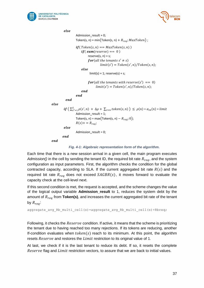
37
𝒆𝒍𝒔𝒆
Admission_result = 0;
Token(s, n) = min(Token(s, n) + 𝑅𝑟𝑒𝑞; 𝑀𝑎𝑥𝑇𝑜𝑘𝑒𝑛) ;
𝒊𝒇( 𝑇𝑜𝑘𝑒𝑛(𝑠, 𝑛) == 𝑀𝑎𝑥𝑇𝑜𝑘𝑒𝑛(𝑠, 𝑛) )
𝒊𝒇( 𝒔𝒖𝒎(𝑟𝑒𝑠𝑒𝑟𝑣𝑒) == 0 )
reserve(s, n) = s;
𝒇𝒐𝒓(𝑎𝑙𝑙 𝑡ℎ𝑒 𝑡𝑒𝑛𝑎𝑛𝑡𝑠 𝑠′ ≠ 𝑠)
𝑙𝑖𝑚𝑖𝑡(𝑠′) = 𝑇𝑜𝑘𝑒𝑛(𝑠′, 𝑛) 𝑇𝑜𝑘𝑒𝑛(𝑠, 𝑛)⁄ ;
𝒆𝒍𝒔𝒆 limit(s) = 1; reserve(s) = s;
𝒇𝒐𝒓(𝑎𝑙𝑙 𝑡ℎ𝑒 𝑡𝑒𝑛𝑎𝑛𝑡𝑠 𝑤𝑖𝑡ℎ 𝑟𝑒𝑠𝑒𝑟𝑣𝑒(𝑠′) == 0)
𝑙𝑖𝑚𝑖𝑡(𝑠′) = 𝑇𝑜𝑘𝑒𝑛(𝑠′, 𝑛) 𝑇𝑜𝑘𝑒𝑛(𝑠, 𝑛)⁄ ;
𝒆𝒏𝒅
𝒆𝒏𝒅
𝒆𝒏𝒅
𝒆𝒍𝒔𝒆
𝒊𝒇 ( ∑ 𝜌(𝑠′, 𝑛)𝑆𝑠′=1 + ∆𝜌 + ∑ 𝑡𝑜𝑘𝑒𝑛(𝑠, 𝑛) 𝑠′≠𝑠 ) ≤ 𝜌(𝑛) ∗ 𝛼𝑡ℎ(𝑛) ∗ 𝑙𝑖𝑚𝑖𝑡
Admission_result = 1;
Token(s, n) = max(Token(s, n) − 𝑅𝑟𝑒𝑞; 0);
𝑅(𝑠)+ = 𝑅𝑟𝑒𝑞;
𝒆𝒍𝒔𝒆
Admission_result = 0;
𝒆𝒏𝒅
𝒆𝒏𝒅
Fig. 4-1: Algebraic representation form of the algorithm.
Each time that there is a new session arrival in a given cell, the main program executes
Admission() in the cell by sending the tenant ID, the required bit rate 𝑅𝑟𝑒𝑞, and the system
configuration as input parameters. First, the algorithm checks the condition for the global
contracted capacity, according to SLA. If the current aggregated bit rate 𝑅(𝑠) and the
required bit rate 𝑅𝑟𝑒𝑞 does not exceed 𝑆𝐴𝐺𝐵𝑅(𝑠) , it moves forward to evaluate the
capacity check at the cell-level next.
If this second condition is met, the request is accepted, and the scheme changes the value
of the logical output variable Admission_result to 1, reduces the system debt by the
amount of 𝑅𝑟𝑒𝑞 from Token(s), and increases the current aggregated bit rate of the tenant
by 𝑅𝑟𝑒𝑞:
aggregate_avg_Rb_multi_cell(s)=aggregate_avg_Rb_multi_cell(s)+Rbreq;
Following, it checks the 𝑅𝑒𝑠𝑒𝑟𝑣𝑒 condition. If active, it means that the scheme is prioritizing
the tenant due to having reached too many rejections. If its tokens are reducing, another
If-condition evaluates when 𝑡𝑜𝑘𝑒𝑛(𝑠) reach to its minimum. At this point, the algorithm
resets 𝑅𝑒𝑠𝑒𝑟𝑣𝑒 and restores the 𝐿𝑖𝑚𝑖𝑡 restriction to its original value of 1.
At last, we check if it is the last tenant to reduce its debt. If so, it resets the complete
𝑅𝑒𝑠𝑒𝑟𝑣𝑒 flag and 𝐿𝑖𝑚𝑖𝑡 restriction vectors, to assure that we are back to initial values.

38
If the RAB request does not pass the capacity check at cell-level condition, the algorithm
rejects the request, so it sets admission_result to 0, and 𝑡𝑜𝑘𝑒𝑛(𝑠) increases by the amount
of 𝑅𝑟𝑒𝑞.
Following the rejection, the algorithm evaluates if the token bucket of tenant 𝑠 has reached
𝑀𝑎𝑥𝑇𝑜𝑘𝑒𝑛. In that case, it activates 𝑅𝑒𝑠𝑒𝑟𝑣𝑒 for tenant 𝑠. If it is the first tenant to activate
it, the 𝐿𝑖𝑚𝑖𝑡 restriction is applied to all other tenants. The limits are calculated within a for-
loop, as a proportion of the differences between the tokens from tenants 𝑠′ different than
𝑠, and the token from the corresponding tenant 𝑠:
limit(s_aux)=token(s_aux)./token(s);
For the condition where more than one tenant has reached its corresponding 𝑀𝑎𝑥𝑇𝑜𝑘𝑒𝑛
threshold, the scheme activates 𝑅𝑒𝑠𝑒𝑟𝑣𝑒 and applies the 𝐿𝑖𝑚𝑖𝑡 restriction, but only to
those tenants with 𝑅𝑒𝑠𝑒𝑟𝑣𝑒 equals to 0.
The second part of the scheme evaluates the admission request when the corresponding
tenant exceeds its contracted SAGBR. Admission to the network at this point is possible,
but the algorithm needs to calculate first the actual debt that the system holds with other
tenants. Next, it evaluates the capacity check at cell-level, but in this case, the request
passes the condition only if the aggregated number of RBs used by all tenants rho_aggr,
plus the RBs required for the new RAB delta_rho and the actual debt from other tenants
token_agg does not exceed the amount of available RBs at the cell. Token_agg must be
expressed in RB units:
token_agg=(sum(token)-token(s))./Rb_estimate_per_RB;
If the request passes the condition, the algorithm sets admission_result to 1, 𝑡𝑜𝑘𝑒𝑛(𝑠)
decreases by the amount of 𝑅𝑟𝑒𝑞, and the overall aggregated bit rate of tenant 𝑠 increases
by 𝑅𝑟𝑒𝑞. For the opposite scenario, the scheme sets admission_result to 0; but there is no
increment of the system’s debt since the tenant already has all its capacity used.

39
5. Results
This chapter presents and analyses the simulation results obtained from using our proposal
for a multi-tenant AC function for future networks. The first part of this section describes
the simulation setup used for all the executed simulations using our algorithm. It then
compares its performance with a baseline scheme and with the scheme presented in 2.3.3.
We use aggregated bit rate, blocking probability, bit rate increase, and system RB
occupation as the performance metrics to evaluate our algorithm.
5.1. Scenario description
The first step is setting the parameters that frame the scenario on which we perform the
simulation. Next, we define values that translate those parameters into the simulation. The
situation where we evaluate our new scheme considers an outdoor Urban Micro scenario,
where an infrastructure provider deploys a multi-tenant RAN, conformed by gNB nodes. To
simplify the analysis without losing generality, we consider N=2 cells, operating with one
frequency carrier of 10 MHz each, which corresponds to 50 RBs per site. Considering the
propagation parameters listed in Table 5.1, the infrastructure provider configures each cell
with an effective capacity of 31 Mbps, considering an empirical correction of 0.7757 (𝜃).
Two tenants lease the deployed NG-RAN, identified as T1 and T2. Both operators have
signed SLAs with the provider; therefore, the agreed capacity for T1 is SAGBR(1) = 25
Mbps, and for T2 is SAGBR(2) = 37 Mbps. With these SAGBR values, the capacity share
for T1 is C(1) = 0.4, and C(2) = 0.6 for T2.
Parameter Value
Inter-Site distance (ISD) 200 m
Path loss model
Urban micro-cell model with a
hexagonal layout
Shadowing standard deviation 3 dB in LOS and 4 dB in NLOS
BS antenna gain 5 dB
Frequency 2.6 GHz
Tx power per RB 24 dBm
RBs per cell 𝜌(𝑛) 50 RBs
Bandwidth per RB 180 KHz
UE noise figure 9 dB
Spectral efficiency model to map SINR 4.4 b/s/Hz
𝑅𝑟𝑒𝑞 1024 Kbps
Session duration Exponential model: 30 s
Session arrival rate
Values from [0.2, 1.2], following a
Poisson model
𝛼𝑡ℎ(𝑛) 1
𝛾, 𝛽, 𝜃 (1.0, 1.0, 0.7757)

40
vector_variation [0.2, 0.4, 0.6, 0.8, 1.0, 1.2]
simulation_duration 50000.0 s
time_step 0.1 s
num_cells 2
num_tenants 2
C(1) 0.4
C(2) 0.6
traffic_params.Rbreq 1024 Kbps
traffic_params.duration 30 s
MaxToken(s) [12.287, 18.430] Mb/s
limit [1, 1]
reserve [0, 0]
Table 5-1: Simulation Parameters. [4]
For practical purposes, we are going to focus on the Downlink direction of the channel. The
NG-RAN receives RAB requests from UEs, which arrive following a Poisson arrival model
that simulates a random behavior. The session duration for these RABs follows an
exponential model.
To test the algorithm under different conditions, we can change the offered loads for each
tenant by varying the session arrival rate 𝜆 in each cell.
The objective is to see if we can increase the available capacity for the participating tenants
by optimizing the usage of resources. We seek to achieve that by reducing the complexity
of the policy processing, while at the same time trying to maintain fairness with the cell
capacity distribution stated in the SLAs. Due to this, we focus on analyzing any bit rate
increase for each tenant and the flexibility of our proposal under different traffic distributions.
We can reach both purposes through the Token(s) concept from (3.3), (3.5).
Consequently, the performance assessment will consider as references two cases. The
case where the same scenario utilizes an AC algorithm denoted as “NoDelta,” that
contemplates network slicing with fixed values for the capacity shares but does not allow
flexibility to re-use unused capacity left by other tenants.
After that, we compare our scheme with the “Delta_C” algorithm presented in 2.3.3, as a
second benchmark for evaluating the bit rate increase and the blocking probability.

41
5.2. Results presentation with the baseline scheme
First, we evaluate our algorithm operating under a range of offered loads for each tenant,
extending from 0 to 80 Mb/s. Upon this matrix of offered loads, we evaluate the aggregated
bit rate obtained by our proposal, and the bit rate obtained by the “NoDelta” algorithm as a
reference. From this comparison, we collect the gain achieved by our algorithm in terms of
the bit rate increase percentage, as a function of the different offered loads for T1 and T2.
The analysis considers the total offered loads on the scenario, as well as the total bit rates,
evenly distributed through all cells.
Fig. 5-1: Bit Rate increase obtained by T1 concerning “NoDelta."
Fig. 5-1 shows the aggregated bit rate increase obtained by T1 with the proposed scheme,
in comparison to the "NoDelta" benchmark. The X-axis is the offered loads for T2, the Y-
axis is the offered loads for T1, and the Z-axis represents the bit rate increase (%). We can
see that, when T2 is using all its capacity (offered loads of around 60, 80 Mb/s), the
improvements for T1 are small, from 24%, 30%. Nevertheless, we can see a peak, when
the offered load of T2 is zero, and the amount of T1 is 73.8 Mb/s, T1 can increase its bit
rate up to 127%, when the proposed scheme reaches a bit rate of 67 Mb/s, compared to
the 29.4 Mb/s achieved with the "NoDelta" scheme.
Fig. 5-2: Bit Rate increase obtained by T2 concerning “NoDelta."

42
For the case of T2, we also have a bit rate increase in terms of the offered loads, as seen
in Fig. 5-2. Even though we see small decreases of bit rate, this happens for offered loads
of zero or close to zero, so we can neglect these differences since they belong to minimal
values. What we do appreciate is the peak for the bit rate increase, of around 51%, when
the offered load of T1 is zero, and T2 can use all the available capacity. T2 reaches 66.9
Mb/s with the proposed algorithm and 44.3 Mb/s with the “NoDelta” scheme. We can see
these improvements thanks to the re-use of resources, which allows increasing the
available capacity for tenants. T1 obtains a more significant benefit since T2 can leave
more unused resources.
Next, we want to see how our scheme performs when handling different traffic distributions
for each tenant. In this way, we can evaluate the flexibility of the algorithm. Considering
this, we assume two different traffic distributions: Traffic A and Traffic B. When the offered
load of a tenant is equal to the contracted value in the SLA, it is marked as planned (P);
when traffic is less than expected it is marked as low (L), and if it is above, is marked high
(H). With this notation, we establish table 5.3:
Traffic Distribution
Tenant Load BS(1)
Not. Load BS(2)
Not. Load Total
Not.
Traffic A T1 24.6 (H) 24.6 (H) 49.2 (H)
T2 12.3 (L) 12.3 (L) 24.6 (L)
Traffic B T1 19 (H) 6 (L) 25 (P)
T2 12 (L) 25 (H) 37 (P)
Table 5-2: Traffic distributions.
We first consider the scenario where T1 is receiving a heavy load of traffic, but T2 is not
using all its capacity. The traffic distribution A tests how the proposed algorithm responds
to these different traffic distributions and the available resources.
Fig. 5-3: Aggregated bit rate and blocking probability by each tenant in the whole scenario;
Traffic A.

43
Fig. 5-3 shows the results for the total aggregated bit rate and total blocking probability
experienced by each tenant by using our algorithm and compared with the “NoDelta”
reference. We observe that the aggregated bit rate for T1 is 44.2 Mb/s, versus the 28 Mb/s
obtained with NoDelta, which shows an increase of 56% in the bit rate of T1. Notice that
T1 is making use of the available capacity from T2, which suffers a small decrease of
around 7% in its bit rate. These results agree with the observed reduction in the blocking
probability from T1, which reduces from 42% to 10%, but the blocking probability of T2
suffers a small increase, to 7%.
We next, consider the scenario where the distribution of traffic varies in each cell. In traffic
distribution B, the offered load of T1 is high while T2 is low in the first cell, but in the
second cell, the offered load of T2 is high, and T1 is low. Although the total offered load of
both tenants corresponds to the planned one, this asymmetry in the traffic tests the
flexibility of the algorithm.
Fig. 5-4: Bit Rate by each tenant in each cell and the total scenario; Traffic B
Fig. 5-4 shows the bit rate obtained by each tenant in each cell and the entire scenario,
using traffic distribution B. We can see that in cell 1, T1 improves its bit rate from 13.5 Mb/s
to 18.5 Mb/s, while T2 remains almost the same. In cell 2, it is T1 that maintains the same
bit rate, and T2 improves from 20 Mb/s to 24.5 Mb/s. These results translate into an
improvement of 23% for T1 and 10% for T2, compared with the “NoDelta” reference.
Next, we review Fig. 5-5, where we depict the blocking probability in each cell and the
whole scenario, also with the traffic distribution B. T1 achieves a significant reduction in
cell 1, from 29% to 3%, at the cost of a small increase in T2, from 0.2% to 3%. In cell 2, it
is T2 who uses the available capacity of T1, reducing its blocking probability from 18% to
3%, with a slight increase in T1, from 0.1% to 3%. These reductions represent a global gain
for both tenants since the total blocking probability of T1 reduces by 84%, and that for T2
reduces by 74%.

44
Fig. 5-5: Blocking probability by each tenant in each cell and the total scenario; Traffic B
5.3. Comparative versus the Delta_C algorithm
After studying the achieved bit rate increases concerning the case of a shared NG-RAN
that does not take advantage of unused capacity left by other tenants, we now examine
the performance of the Tokens(s) term. We check if it enhances the operation of the AC
function concerning the ∆𝐶(𝑠, 𝑛) term from the scheme presented in section 2.3.3.
First, we evaluate the results obtained for the absolute values of bit rate and blocking
probability, and then we analyze the flexibility of the schemes with the traffic distribution B.
Fig. 5-6: Bit rate and blocking probability obtained with the proposed algorithm and with
the Delta_C reference; Traffic A
In this case, fig. 5-6 shows a comparison in the gains of bit rate and blocking probability,
between our proposal and the AC algorithm of section 2.3.3. Both schemes improve the bit
rate concerning the “NoDelta” reference. Still, in this case, we see that by having fewer
parameters and conditions to analyze, our proposal achieves an improvement in the use

45
of resources, and at the same time, maintain fairness with the distribution of capacity for
tenants. Using traffic distribution A, T1 achieves a total bit rate of 44 Mb/s with the proposed
scheme, compared to the 37 Mb/s obtained with the “Delta_C” scheme, but with a slight
degradation in the bit rate of T2, from 24.2 Mb/s to 22.6 Mb/s. The proposed algorithm
obtains a total improvement of 17% in the bit rate compared to the reference, and only a
small reduction in the bit rate of T2. T1 also achieves a significant decrease in its blocking
probability, of 53%, due to a higher amount of spare capacity left by T2, at the cost of a
small increase in the blocking probability of T2.
Fig. 5-7: Bit Rate in each cell and the total scenario with the proposed algorithm and with
the Delta_C reference; Traffic B
With traffic distribution B, we want to measure the flexibility of the algorithms under different
offered loads. Fig. 5-7 depicts the bit rates achieved by both schemes, in each cell and the
entire scenario. The proposed algorithm makes an improvement for T1 in cell 1, although
it suffers a reduction for T2. In cell 2, the opposite occurs since the distribution of offered
loads is (L) for T1 and (H) for T2. Finally, we observe an increase in the global scenario of
4.6% in the bit rate of T1 and 2% in the bit rate of T2, respect to the “Delta_C” reference.
Fig. 5-8: Blocking probability in each cell and the total scenario with the proposed
algorithm and with the Delta_C reference; Traffic B

46
Finally, we assess the flexibility of the schemes by analyzing the blocking probabilities
obtained in each cell and the whole scenario. In fig. 5-8, we notice that the proposed
algorithm has higher flexibility when managing the unused resources that each tenant
leaves since in cell 1, where traffic load is (H) for T1 and (L) for T2, we see that T1 achieves
a significant reduction in its blocking probability when using the proposed scheme. In cell
2, where traffic load is (L) for T1 and (H) for T2, we observe that T2 is who has a higher
reduction when it also uses the proposed scheme. We conclude that our algorithm handles
the available resources more efficiently, allowing a reduction in the total scenario of 61%
for T1, and 33% for T2.
5.4. Impact of algorithm parameters
In this section, we are focused on the effect of the algorithm parameters on its performance
under different traffic loads. To accomplish this, we will carry out the study only with results
from this algorithm, considering some values of selected traffic loads. First, we study the
dynamic evolution of the Tokens(s) term throughout a simulation. We examine the effect
of the minimum and maximum values assigned to the Tokens(s) term and its impact on the
operation of the AC function. Finally, we assess the importance of the 𝑅𝑒𝑠𝑒𝑟𝑣𝑒 flag and its
relation to the 𝑀𝑎𝑥𝑇𝑜𝑘𝑒𝑛 value.
Dynamic Token evolution
We have already expressed in section 3.2 that the Tokens(s) term represents the system's
debt to the tenant. When the tenant RABs are accepted, the amount of tokens reduces,
and the tenant increases its aggregated bit rate 𝑅(𝑠). When the AC function rejects the
required bit rate 𝑅𝑟𝑒𝑞, only the amount of tokens increases.
Based on this definition, we find two characteristics in the behavior of the tokens:
1. When the tokens increase, it does not mean that the tenant's 𝑅(𝑠) decreases.
2. When the tokens decrease, it is because the system accepts RABs of the tenant
again. So as a consequence, the aggregated bit rate 𝑅(𝑠) has to increase.
To study the dynamic evolution of the tokens, we will include the development of the bit
rate admitted for each tenant. We consider two different distributions of offered load: The
first distribution examines Traffic B, that presents the distribution (H) and (L) in cell 1 and
(L) and (H) in cell 2; the second distribution considers 𝜆(1) and 𝜆(2) = 0.8 equally
distributed between the cells.
The first distribution assists to show the flexibility of the term Tokens(s) under different
traffic distributions.
The dynamic tokens evolution for each tenant during the complete simulation, along with
the corresponding aggregated bit rate evolution, are illustrated in fig. 5-9. In (a), the
instantaneous bit rates of T1 and T2 are represented respectively, for each 0.1-sec
time_step, throughout the 50,000-second simulation, for cell 1. In (b), it is described the
same for cell 2.
We notice that the one tenant with the highest offered traffic load, uses more cell resources,
so it employs fewer tokens than the opposite tenant. In cell 2, the traffic distribution is (L)
vs. (H), so T1 uses its tokens several times, reaching 3 Mb/s, while T2 does not.

47
Distribution 1: 𝜆(1,1)=0.62, 𝜆(1,2)=0.39, 𝜆(2,1)=0.2, 𝜆(2,2)=0.82 (TRAFFIC B)
(a)
(b)
Fig. 5-9: Bit rate and Tokens evolution during the complete simulation: (a) cell1, and (b) cell2.
Fig. 5-10: Zoom of 200 seconds in the bit rate and token graphs, cell 1.
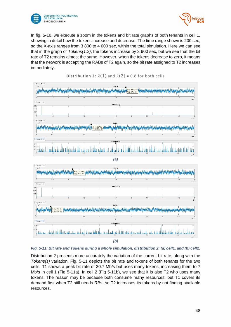
48
In fig. 5-10, we execute a zoom in the tokens and bit rate graphs of both tenants in cell 1,
showing in detail how the tokens increase and decrease. The time range shown is 200 sec,
so the X-axis ranges from 3 800 to 4 000 sec, within the total simulation. Here we can see
that in the graph of Tokens(1,2), the tokens increase by 3 900 sec, but we see that the bit
rate of T2 remains almost the same. However, when the tokens decrease to zero, it means
that the network is accepting the RABs of T2 again, so the bit rate assigned to T2 increases
immediately.
Distribution 2: 𝜆(1) and 𝜆(2) = 0.8 for both cells
(a)
(b)
Fig. 5-11: Bit rate and Tokens during a whole simulation, distribution 2: (a) cell1, and (b) cell2.
Distribution 2 presents more accurately the variation of the current bit rate, along with the
Tokens(s) variation. Fig. 5-11 depicts the bit rate and tokens of both tenants for the two
cells. T1 shows a peak bit rate of 30.7 Mb/s but uses many tokens, increasing them to 7
Mb/s in cell 1 (Fig 5-11a). In cell 2 (Fig 5-11b), we see that it is also T2 who uses many
tokens. The reason may be because both consume many resources, but T1 covers its
demand first when T2 still needs RBs, so T2 increases its tokens by not finding available
resources.

49
Fig. 5-12: Zoom of 200 seconds in the bit rate and token graphs during dist. 2, cell 1.
We make a zoom at the graphs in cell 2, to analyze the bit rate and tokens of both tenants
during the range of 39 500 – 39 700 sec. During that period, we focus on the tokens of T2,
which star to increase from the 39 620 sec. We can observe that when the tokens increase,
the bit rate of T2 is low, matching with a high peak in the bit rate of T1. Once the tokens
begin to decline, the bit rate of T2 increases significantly, and the bit rate of T1 drops,
proving the flexibility of the algorithm to reallocate resources among tenants.
Impact of Minimum and Maximum Tokens values
In the previous simulations, we have seen the behavior of the tokens under different traffic
loads. We understand that the Tokens(s) term helps increase the bit rate and improve the
flexibility of the algorithm. Still, now we are going to review the effect of varying the limits
of the values of the token bucket.
- According to the agreements made with the infrastructure provider, there should
not be a network debt with the MNOs, so under normal conditions, the minimum
token value should always be zero.
- It is the maximum threshold that affects the behavior of the algorithm, and
consequently, the performance of the cell and the QoS experienced by all the
involved users.
Initially, we configure the algorithm with the threshold 𝑀𝑎𝑥𝑇𝑜𝑘𝑒𝑛 = 𝑐𝑒𝑙𝑙𝑆𝐴𝐺𝐵𝑅(𝑠), since
we establish that under no circumstance should the system debt exceed the total
contracted capacity of the cell of the tenant. Nevertheless, analyzing the Tokens graphics
under distribution 1 (Fig. 5-9), we see that the token pile only increases up to values of 6
Mb/s despite receiving high traffic loads, and being MaxToken(1)=12.3 Mb/s, and
MaxToken(2)=18.4 Mb/s respectively. As a consequence, the Reserve condition does not
become active. This situation is because the RBs occupation is set at 38.3 in cell 1 and
38.5 in cell 2.
𝑀𝑎𝑥𝑇𝑜𝑘𝑒𝑛 serves to restrict the system's debt, and this happens when the cell becomes
saturated. Consequently, we must analyze these cases where the base station reaches
the limit of its capacity. This saturation may occur when several tenants share the NG-RAN
(N > 2), or when the tenants receive a very high traffic load, for example in very particular

50
conditions such as seasonal events, concerts or football matches. To simplify our
simulations, we will continue using N = 2 tenants, but we will consider very high traffic loads,
with 𝜆(1) and 𝜆(2) = 2.0.
First, we limit MaxToken to 25% of 𝑐𝑒𝑙𝑙𝑆𝐴𝐺𝐵𝑅(𝑠), considering more accurate agreed
saturation values for a mobile network, and from there we extend the possible system debt
with 𝑀𝑎𝑥𝑇𝑜𝑘𝑒𝑛 to the 100% of𝑐𝑒𝑙𝑙𝑆𝐴𝐺𝐵𝑅(𝑠); we obtain the following results:
Fig. 5-13: System blocks by each cell; with 0.25 and full MaxToken
Fig. 5-14: Blocking probability by each tenant in each cell; with 0.25 and full MaxToken
Reviewing the operating parameters of the cells, we observe in Fig. 5-13 that when the
system restricts its debt to 0.25 ∗ 𝑐𝑒𝑙𝑙𝑆𝐴𝐺𝐵𝑅(𝑠) , the number of rejected sessions
decreases. T1 remains at a similar value, but T2 does perceive a meaningful reduction.
Both reductions translate into improvements in the blocking probability for each tenant in
Fig. 5-14, where we observe that although the excessive load of traffic saturates the
tenants, both T1 and T2 achieve a reduction when using 0.25 ∗ 𝑐𝑒𝑙𝑙𝑆𝐴𝐺𝐵𝑅(𝑠) vs. full
𝑐𝑒𝑙𝑙𝑆𝐴𝐺𝐵𝑅(𝑠), in both cells.

51
From the obtained data, we can conclude that the importance of the 𝑀𝑎𝑥𝑇𝑜𝑘𝑒𝑛 value
appears when:
- In particular situations with massive loads of traffic for the tenants, the proposed
algorithm performs very well from the perspective of the tenants, since the bit rate
and blocking probability values do not vary much.
- In similar situations, 𝑀𝑎𝑥𝑇𝑜𝑘𝑒𝑛 becomes valuable when we see the performance
of the cells from the perspective of the infrastructure provider. With 𝑀𝑎𝑥𝑇𝑜𝑘𝑒𝑛, it
is possible to reduce the number of requests blocked and blocking probability in
each cell, which matters a lot for the provider since being able to manage these
Values helps control the levels of QoS offered by the network to all users.
Impact of using 𝑹𝒆𝒔𝒆𝒓𝒗𝒆
In section 3.2, the description of the algorithm presents 𝑀𝑎𝑥𝑇𝑜𝑘𝑒𝑛 as the maximum value
to which the system's debt can rise. This term works directly with the 𝑅𝑒𝑠𝑒𝑟𝑣𝑒 and 𝐿𝑖𝑚𝑖𝑡
restriction because when MaxToken is activated, 𝑅𝑒𝑠𝑒𝑟𝑣𝑒 is also enabled to control the
allocation of RBs to tenants. According to this, we conclude that the limitation does not
influence directly into the capacity received by the tenants. Still, it does help to handle the
RBs better to avoid cell congestion.
Fig. 5-15: Congestion probability per cell, using Limit vs. NoLimit.
Fig. 5-16: RB occupation per cell, using Limit vs. NoLimit.
52
Fig. 5-15 depicts the congestion probability for each cell when excessive traffic load is
received (𝜆(1) = 𝜆(2) = 2.0), using the complete algorithm with 25% of 𝑀𝑎𝑥𝑇𝑜𝑘𝑒𝑛 and
100% 𝑀𝑎𝑥𝑇𝑜𝑘𝑒𝑛, and comparing it with a version without the 𝐿𝑖𝑚𝑖𝑡 restriction.
As we had already mentioned, when 𝑀𝑎𝑥𝑇𝑜𝑘𝑒𝑛 = 𝑐𝑒𝑙𝑙𝑆𝐴𝐺𝐵𝑅(𝑠), the system accepts
very high values of debt, so 𝑅𝑒𝑠𝑒𝑟𝑣𝑒 and 𝐿𝑖𝑚𝑖𝑡 are not activated, and performance is the
same using the algorithm with or without 𝐿𝑖𝑚𝑖𝑡 . The effect of the restriction is best
observed when comparing the proposed algorithm with 25% of 𝑀𝑎𝑥𝑇𝑜𝑘𝑒𝑛 , with the
algorithm without 𝐿𝑖𝑚𝑖𝑡 and 25% of 𝑀𝑎𝑥𝑇𝑜𝑘𝑒𝑛. In this way, we find in cell 1 that using the
restriction reduces the congestion probability from 11.2% to 10.7%, and from 11.12% to
10.6% in cell 2.
Likewise, the use of RBs in Fig. 5-16 is improved, where using 𝐿𝑖𝑚𝑖𝑡 and 0.25 ∗
𝑀𝑎𝑥𝑇𝑜𝑘𝑒𝑛, a decrease of 48.61 to 48.5 is achieved in the occupancy of RBs in cell 1, and
from 48.62 to 48.5 in cell 2.
A lower congestion probability and less occupation of RBs is beneficial for operators, not
directly as throughput, but in the quality of service delivered to all sessions attended.

53
6. Budget
In this section, we present the costs associated with the development of a research project
on a new AC algorithm.
A single person, with a degree in telecommunications engineering, has executed the
project. The approximate value of cost per labor [€/h] is assigned, equivalent to the
expenses of a junior engineer, and the time of dedication for implementing the project,
considering all the stages, as well as planning, research, implementation, simulations, and
conclusion of the project. Table 6-1 summarizes the obtained costs:
Table 6-1: total project costs
The time dedication considers 30 hours of work per week for 25 weeks, which gives us 750
hours of total employment. As a consequence, the total cost for the entire project is a total
of 7 500 EUR.
Regarding the costs related to the material used, the use of a MATLAB license, valued at
500 EUR, is considered. However, since we developed the project under the supervision
of the university, we used a license provided by the administration, which absorbs these
costs.
Personnel Salary [€/h] Task hours Total cost
Junior Engineer 10.00 € Bibliographic study 100 1,000.00 €
Implementation of algorithm 150 1,500.00 €
Simulation 200 2,000.00 €
Memory elaboration 300 3,000.00 €
Total 750 7,500.00 €

54
7. Conclusions and future development
This chapter concludes the presented research work of this thesis. We offer a summary of
the investigation, along with some conclusions we arrived after completing the analysis of
the results.
We have studied the considerable impact that future networks bring, and how the current
telecommunications landscape will change with the implementation of technologies such
as 5G, IoT, and M2M. Due to this, it is crucial to implement all the tools that can provide us
with the advantages and capabilities of future networks, such as Network Slicing, SDN,
and edge computing.
Throughout this work, we have presented a detailed review of future networks, Multi-
tenancy, and the operation of the Admission Control under this scenario, with the focus on
increasing available capacity for tenants by implementing a policy simpler to use and
capable of managing the end-to-end QoS through the network. Consequently, we propose
a new Admission Control algorithm based on Tokens, which we design using the traffic
policy of Token-bucket as motivation. This mechanism provides the simplicity and fairness
of the algorithm. To this end, the algorithm relies on two control conditions: the global
contracted capacity condition, and the capacity check at the cell-level. On the first check,
the algorithm ensures that the requests met the SLA agreements fairly. The latter check
guarantees that the cell has sufficient capacity to accept incoming connection requests.
The motivation for this work was to find an enhanced scheme capable of increase the
usage ratio of physical resources, which should lead to a higher capacity for tenants. After
designing the proper algorithm, we performed a simulation-based analysis to evaluate the
performance of our scheme under a multi-tenant, multi-cell NG-RAN for future networks.
The assessment focused on analyzing the bit rate increase for each tenant and
examinating the flexibility of the algorithm under different traffic distributions. Simulation
results show that our proposal can obtain a bit rate of 67 Mb/s, which translates into a bit
rate increase of 127% concerning the “NoDelta” scenario, and a bit rate increase of 17%,
when comparing the achieved 44.2 Mb/s, vs. the 37.7 Mb/s obtained with the “Delta_C”
reference.
The algorithm proves its flexibility by reducing the blocking probability, and our proposal
obtains substantial reductions from the “NoDelta” benchmark. Still, it also makes significant
reductions when comparing to the “Delta_C” reference, decreasing from 42% to 10.5%
when the distribution of traffic is homogeneous, and from 22% to 3% when the load is
uneven at each cell.
Throughout all the simulations performed, we have been able to evaluate the behavior of
the multiple tenants by sharing the same NG-RAN and how they respond to different traffic
loads. Since the Tokens(s) term provides its flexibility to the algorithm, we focus on
analyzing its dynamic evolution throughout all simulations.
We notice that when the offered load of the entire cell is low, tenants do not use tokens. As
the total cell load increases, the tenant that receives the highest traffic load is the one that
makes more connection requests, so it is usually the tenant with the lowest traffic that finds

55
less available resources in the cell. Therefore it has to increase its token account more.
We establish this behavior as selfish: the one who receives the most traffic uses the most
resources. However, we find that the overall benefit is more significant, since it optimizes
the re-use of resources, and increases the available capacities of all tenants.
Thanks to the results graphics, we can determine how to properly configure the parameters
of the algorithm 𝑀𝑎𝑥𝑇𝑜𝑘𝑒𝑛 and 𝑅𝑒𝑠𝑒𝑟𝑣𝑒 , which play an essential role in helping to
manage the behavior of the cells, controlling the congestion probability and occupancy of
RBs when they approach the limit. 𝑀𝑎𝑥𝑇𝑜𝑘𝑒𝑛 serves as a limit value that protects the
network. When its value is very high, the 𝑅𝑒𝑠𝑒𝑟𝑣𝑒 restriction is not activated, since
𝑀𝑎𝑥𝑇𝑜𝑘𝑒𝑛 allows the system debt to be high. Nevertheless, once correctly configured,
𝑅𝑒𝑠𝑒𝑟𝑣𝑒 will be enabled to manage the resources available to other tenants. Thereby, it
benefits the network operation, avoiding saturation of the cells or degradation in the QoS
of the involved.
The focus of this work has been to optimize the usage of radio resources. However, the
requirements of 5G services also require other resources, such as computational, storage,
and networking elements. Based on these needs, future research possibilities emerge to
satisfy future services completely. As future work, the optimization of the AC function must
be studied along with the optimization of the packet scheduling function, with a higher focus
on its operation under the whole multi-cell RAN scenario.
Finally, in the results, we have seen the importance of 𝑀𝑎𝑥𝑇𝑜𝑘𝑒𝑛 and 𝑅𝑒𝑠𝑒𝑟𝑣𝑒 when
controlling cell performance when the traffic load levels are high. These values must be
analyzed together with the blocking probability of tenants, trying to find a trade-off between
cell performance and offered capacity to operators. One possible improvement could be
introducing an adaptive 𝑀𝑎𝑥𝑇𝑜𝑘𝑒𝑛 value.

56
Bibliography
[1] GSMA. “Charting the Course to 5G.” 2019 [Online]. Retrieved May 29, 2019, from https://www.gsma.com/futurenetworks/technology/understanding-5g/5g-innovation/
[2] GSM Alliance. (2017). An Introduction to Network Slicing. White Paper.
[3] Kwan, R., Arnott, R., & Kubota, M. “On radio admission control for LTE systems.”
In IEEE Vehicular Technology Conference, (1), 1–5.
https://doi.org/10.1109/VETECF.2010.5594566
[4] Pérez-Romero, J., Sallent, O., Ferrús, R., & Agustí, R. “Admission Control for multitenant radio access networks.” In IEEE International Conference on Communications Workshops (ICC Workshops), Paris, 2017, pp. 1073-1078. Doi: 10.1109/ICCW.2017.7962801
[5] Khan, N. K., & Hamdan, A. A. “ITU-T Future Networks : A Step towards Green Computing.” In Proceedings of the World Congress on Engineering and Computer Science 2014 Vol. I. WCECS 2014, 22-24 October 2014, San Francisco, USA.
[6] ITU-T. “Focus Group on Future Networks (FG FN),” 2019 [Online]. Retrieved June 10, 2019, from https://www.itu.int/en/ITU-T/focusgroups/fn/Pages/Default.aspx
[7] Editors. “Draft Deliverable on “Future Networks: Design Goals and Promising Technologies” Focus Group on Future Networks - FG-FN OD-72 Rev.1, December 2010.
[8] GSMA. “Future Networks,” 2019 [Online]. Retrieved May 29, 2019, from https://www.gsma.com/futurenetworks/
[9] GSMA. “Engage with Future Networks,” 2019 [Online]. Retrieved May 29, 2019, from https://www.gsma.com/futurenetworks/about-us/
[10] GSMA. “Technology”, 2019 [Online]. Retrieved May 29, 2019, from https://www.gsma.com/futurenetworks/technology/
[11] GSMA. “RCS Business Messaging,” 2019 [Online]. Retrieved May 30, 2019, from https://www.gsma.com/futurenetworks/technology/enriched-calling-with-rcs/
[12] GSMA. “RCS Market”, 2019 [Online]. Retrieved May 30, 2019, from https://www.gsma.com/futurenetworks/rcs/rcs-market/
[13] J M Meredith. “NR: 3GPP’s 5G radio access technology”. 3GPP presentation, April 2018.
[14] 3GPP TR 29.915 v1.1.0 “Release 15 Description; Summary of Rel-15 Work Items (Release 15)”, March 2019

57
[15] E Borcoci. “End-to-end, multi-domain and multi-tenant aspects in 5G network slicing”. Presentation. University Politehnica Bucharest. Softnet 2018 Conference, October 14 - 18, Nice.
[16] Dahlman, E., & Parkvall, S. "NR - The new 5G radio-access technology". IEEE Vehicular Technology Conference, 2018-June, 1–6. https://doi.org/10.1109/VTCSpring.2018.8417851
[17] NR; NR and NG-RAN Overall Description; Stage 2 (Release 15). 3GPP TS 38.300 V15.5.0, March 2019.
[18] 5G Americas. “5G Network transformation”. December 2017.
[19] Service Aspects and Requirements for Network Sharing, Rel.10. 3GPP TR 22.951 May 2011.
[20] Network Sharing; Architecture and Functional Description, Rel. 12. 3GPP TS 23.251, March 2015.
[21] Study on RAN Sharing Enhancements, Rel.13. 3GPP TR 22.852, September 2014.
[22] Afolabi, I., Taleb, T., Samdanis, K., Ksentini, A., & Flinck, H. “Network slicing and softwarization: A survey on principles, enabling technologies, and solutions.” IEEE Communications Surveys and Tutorials, 20(3), 2429–2453, March 2018. https://doi.org/10.1109/COMST.2018.2815638
[23] 5G-PPP Architecture Working Group. “5G-PPP White Paper on 5G Architecture”. December 2017, 140. https://doi.org/10.13140/RG.2.1.3815.7049
[24] GSMA. “Network Slicing.” 2019 [Online]. Retrieved May 29, 2019, from understanding-
5g/network-slicing/. Website:
https://www.gsma.com/futurenetworks/technology/understanding-5g/network-slicing/
[25] Han, B., Sciancalepore, V., Feng, D., Costa-Perez, X., & Schotten, H. D. “A Utility-
Driven Multi-Queue Admission Control Solution for Network Slicing.” (January 2019).
Retrieved from http://arxiv.org/abs/1901.06399
[26] Han, B., Dedomenico, A., Dandachi, G., Drosou, A., Tzovaras, D., Querio, R.,
Schotten, H. D. “Admission and Congestion Control for 5G Network Slicing”. In 2018
IEEE Conference on Standards for Communications and Networking, CSCN 2018.
https://doi.org/10.1109/CSCN.2018.8581773.
[27] Qian, M., Huang, Y., Shi, J., Yuan, Y., Dutkiewicz, E. “A novel radio Admission Control
scheme for multiclass services in LTE systems.” In GLOBECOM - IEEE Global
Telecommunications Conference, 2.
[28] Elayoubi, S. E., Jemaa, S. Ben, Altman, Z., & Galindo-Serrano, A. “5G RAN Slicing for
verticals: Enablers and challenges”. IEEE Communications Magazine, 57(1), 28–34,
2019. https://doi.org/10.1109/MCOM.2018.1701319.
[29] T. Guo, R. Arnott. "Active LTE RAN Sharing with Partial Resource Reservation." IEEE
VTC Fall, Las Vegas, Sep. 2013. https://doi.org/10.1109/VTCFall.2013.6692075

58
[30] Holma, H., Toskala, A. WCDMA for UMTS – HSPA evolution and LTE, 4th ed. West Sussex, England: John Wiley & Sons, 2007.
[31] 3GPP TS 36.300 v13.2.0 “E-UTRA and E-UTRAN Overall description; Stage 2 (Release 13)”, December 2015
[32] Gutierrez-Estevez, D. M., Bulakci, O., Ericson, M., Prasad, A., Pateromichelakis, E., Belschner, J., Calochira, G. "RAN enablers for 5G Radio Resource Management". IEEE Conference on Standards for Communications and Networking, CSCN 2017, 1–6. https://doi.org/10.1109/CSCN.2017.8088589
[33] An Architecture for Differentiated Services. IETF RFC 2475, December 1998.
[34] Jha, S., & Hassan, M. Engineering Internet QoS. Massachusetts, USA: Artech House, inc, 2002.
.

59
Glossary
A list of all acronyms and what they stand for.
3GPP 3rd Generation Partnership Project
5G 5th Generation wireless systems
5GC 5th Generation Core Network
AC Admission Control
AMF Access and Mobility Function
CBR Constant Bit Rate
CoMP Coordinated Multipoint Connectivity
DC Dual Connectivity
DiffServ Differentiated services
eMBB Enhanced Mobile Broadband
EPC Evolved Packet Core
E-RAB evolved-Radio Access Bearer
FG Focus Group
FN Future Network
FR1 Frequency Range 1
FR2 Frequency Range 2
GSM Global System for Mobile Communications
GSMA the GSM Association
GST Generic Slice Template
IntServ Integrated services
ITU International Telecommunications Union
ITU-T ITU Telecommunication Standardization Sector
KPI Key Performance Indicator
LTE Long Term Evolution; the 4th generation wireless system
SG Study Group
SLA Service Level Agreement
SlaaS Slice as a Service
MANO Management & Orchestration
MIMO Multiple Input Multiple Output
MME Mobility Management Entity
mMTC Massive Machine-Type Communications
MNO Mobile Network Operator

60
MOP Master Operator
MOP-NM MOP-Network Manager
ng-eNB Next-Generation Enhanced 4G base station.
NFV Network Function Virtualization
NFVI Network Function Virtualization Infrastructure
NFVO Network Function Virtualization Orchestrator
NG-RAN Next Generation Radio Access Network
NSA Non-Stand-Alone
NSB Network Slice Broker
NSI Network Slice Instance
NVS Network Virtualization Substrate
OFDM Orthogonal Frequency-Division Multiplexing
PLMN Public Land Mobile Network
POP Participating Operators
POP-NM POP-Network Manager
QoS Quality of Service
RAB Radio Access Bearer
RAN Radio access network
RB Resource Block
RBG Resource Block Group
RCS Rich communication services
RMSC Multitenant cell Slicing Controller
RRM Radio Resource Management
SA Stand-Alone
SAGBR Scenario Aggregated Guaranteed Bit Rate
SDN Software Defined Networking
SD-RAN Software-Defined RAN
SMF Session Management Function
TTI Transmission Time Interval
UE User Equipment
UMTS Universal Mobile Telecommunications System
UPF User Plane Function
URLLC Ultra-reliable Low-latency Communications
VBR Variable Bit Rate

61
VIM Virtualized Infrastructure Manager
VM Virtual Machine
VMM Virtual Machine Monitor
VNF Virtual Network Function
VNFM Virtual Network Function Manager
Xn Network Interface between NG-RAN nodes