multidimensional data modeling for complex...

Multidimensional Data Modelingfor Complex Data

Torben Bach Pedersen and Christian S. Jensen

November 13, 1998

TR-37

A TIMECENTER Technical Report

Title Multidimensional Data Modeling for Complex Data

Copyright c� 1998 Torben Bach Pedersen and Christian S. Jensen. Allrights reserved.

Author�s� Torben Bach Pedersen and Christian S. Jensen

Publication History March 1999. In Proceedings of ICDE ’99November 1998. A TIMECENTER Technical Report.

TIMECENTERParticipants

Aalborg University, DenmarkChristian S. Jensen (codirector), Michael H. B¨ohlen, Renato Busatto, Curtis E. Dyreson,Heidi Gregersen, Dieter Pfoser, SimonasSaltenis, Janne Skyt, Giedrius Slivinskas,Kristian Torp

University of Arizona, USARichard T. Snodgrass (codirector), Sudha Ram

Individual participantsAnindya Datta, Georgia Institute of Technology, USAKwang W. Nam, Chungbuk National University, KoreaMario A. Nascimento, State University of Campinas and EMBRAPA, BrazilKeun H. Ryu, Chungbuk National University, KoreaMichael D. Soo, University of South Florida, USAAndreas Steiner, TimeConsult, SwitzerlandVassilis Tsotras, Polytechnic University, USAJef Wijsen, Vrije Universiteit Brussel, Belgium

For additional information, see The TIMECENTER Homepage:URL: <http://www.cs.auc.dk/research/DBS/tdb/TimeCenter/>

Any software made available viaTIMECENTER is provided “as is” and without any express or implied war-ranties, including, without limitation, the implied warranty of merchantability and fitness for a particularpurpose.

The TIMECENTER icon on the cover combines two “arrows.” These “arrows” are letters in the so-calledRunealphabet used one millennium ago by the Vikings, as well as by their precedessors and successors.The Rune alphabet (second phase) has 16 letters, all of which have angular shapes and lack horizontal linesbecause the primary storage medium was wood. Runes may also be found on jewelry, tools, and weaponsand were perceived by many as having magic, hidden powers.

The two Rune arrows in the icon denote “T” and “C,” respectively.

Abstract

Systems for On-Line Analytical Processing (OLAP) considerably ease the process of analyzing busi-ness data and have become widely used in industry. OLAP systems primarily employ multidimensionaldata models to structure their data. However, current multidimensional data models fall short in theirability to model the complex data found in some real-world application domains. The paper presentsnine requirements to multidimensional data models, each of which is exemplified by a real-world, clin-ical case study. A survey of the existing models reveals that the requirements not currently met includesupport for many-to-many relationships between facts and dimensions, built-in support for handlingchange and time, and support for uncertainty as well as different levels of granularity in the data. Thepaper defines an extended multidimensional data model, which addresses all nine requirements. Alongwith the model, we present an associated algebra, and outline how to implement the model using rela-tional databases.

1 Introduction

With the continued advances in the underlying hardware technologies for on-line mass storage and therecent focus on data warehousing, the notion of On-Line Analytical Processing (OLAP) [5] is attractingincreasing interest, as business managers attempt to extract useful information from large on-line databasesin order to make informed management decisions.

Reports indicate that traditional data models, such as the ER model [2] and the relational model, do notprovide good support for OLAP applications. As a result, new data models based on amultidimensionalview of data have emerged. These multidimensional data models typically categorize data as beingmea-surable business facts(measures) ordimensions, which are mostly textual and characterize the facts. Forexample, in a retail business,productsare sold tocustomersat certaintimesin certainamountsat certainprices. A typical fact would be apurchase, with the amount and price as the measures, and the customerpurchasing the product, the product being purchased, and the time of purchase as the dimensions.

In OLAP research, most work has concentrated on performance issues; and higher-level issues, such asconceptual modeling, have received less attention. Several researchers have pointed to this lack in OLAPresearch, and it has been suggested to try to combine the traditional OLAP virtues of performance with themore advanced data model concepts from the field ofscientific and statistical databases[9]. This appearsto be a very valuable direction, as it is necessary to put more semantics into the database schema to supportthe typical OLAP style of working directly with the data instead of using pre-formatted reports.

A data model for OLAP applications should have certain characteristics in order to support the complexdata found in many real-world systems. We present nine advanced requirements that a multidimensionaldata model should satisfy and illustrate the requirements using a real-world case study from the clinicalworld. We present an extended multidimensional data model that addresses all nine requirements. Thedata model supports modeling explicit hierarchies in the dimensions, to aid the user in navigating the data.Multiple hierarchies in each dimension is supported, to allow for different aggregation paths, and the non-strict hierarchies found in real-world dimensions, i.e., where a dimension item may have several parents,are also supported. The model treats dimensions and measures symmetrically, to allow measures to be usedas dimensions and vice versa. Many-to-many relationships between facts and dimensions can be captureddirectly in the model, which is important as these relationships often occur in real-world data, e.g., a patientmay have several diagnoses. The data model supports getting correct results when aggregating data, e.g.,data will not be double-counted and non-additive data cannot be added. Data change over time, so supportfor handling change and time is part of the model. Aspects of the uncertainty often associated with data arealso handled by the model. Finally, the model supports handling data with different levels of granularity,which is a need in some applications.

1

The model is equipped with an algebra that is closed and at least as strong as relational algebra withaggregation functions. Finally, we outline how the model can be implemented using relational databases.

Eight previously proposed data models, which are representative for the spectrum of multidimensionaldata models, are evaluated against the nine requirements, and it is shown that no other model satisfies morethan four of these requirements. Importantly, no other model supports many-to-many relationships betweenfacts and dimensions, handling of uncertainty, and different levels of granularity at all, and no other modelcompletely supports handling change and time or non-strict hierarchies.

The presentation is structured as follows. Section 2 sets the stage by first presenting a real-world casestudy from the clinical world together with nine requirements to multidimensional data models; it thendescribes and evaluates previously proposed models against the requirements. Section 3 proceeds to firstdefine the basic extended multidimensional data model, using examples from the case study for illustration,then adds support for handling time and uncertainty to the model. With the data structures of the modelavailable, Section 4 defines an algebra for the model and discusses its properties. Section 5 evaluates themodel against the requirements, and Section 6 summarizes and points to future directions. An appendixoutlines how to implement the model using relational databases.

2 Motivation

This section illustrates the shortcomings of the previously proposed multidimensional models. First, wepresent a case study that shows some of these limitations. The case is taken from the domain of healthcare,where we look at patients, their diagnoses, and their place of residence. Second, we list the requirementsfor features that a data model should satisfy in order to meet the needs of the case study. Third, we relatethese requirements to the existing multidimensional data models.

2.1 A Case Study

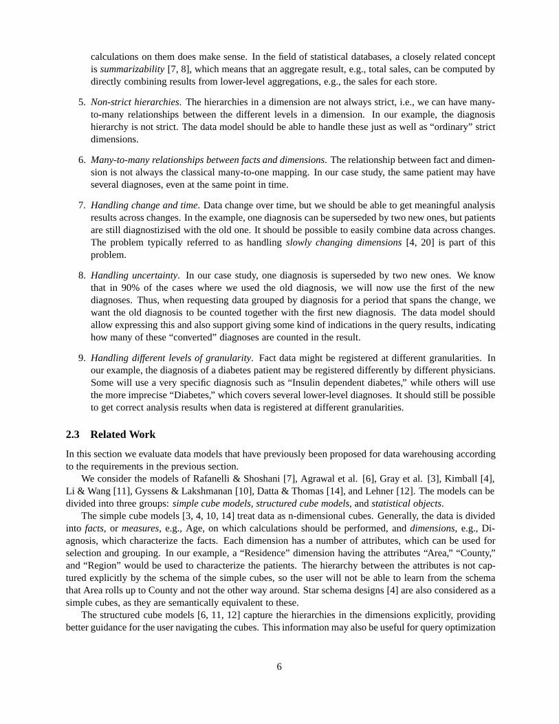
The case study concerns the patients in a hospital, their associated diagnoses, and their place of residence.The goal is to investigate whether some diagnoses occur more often in some areas than in others, in whichcase environmental or lifestyle factors might be contributing to the disease pattern. An ER diagram illus-trating the underlying data is seen in Figure 1.

The most important entities are thepatients. For a patient, we record Name, Social Security Number(SSN), and Date of Birth. From the Date of Birth and the current date, we can derive the Age attribute,which is parenthesized to show that it is derived.

Each patient can have one or morediagnoses. The attribution of diagnoses to patients can vary overtime, and we also record the time interval where a diagnosis is considered to be valid for a patient. We alsorecord thetype of diagnostization, to show whether a diagnosis is considered to beprimary or secondary. Aprimary diagnosis is considered to be the most important reason for a treatment, while secondary diagnosescomplete the view of the patient’s condition. A patient may have only one primary diagnosis at any onepoint in time.

When registering a diagnosis of a patient, physicians often use different levels of granularity. Somewill use the very precise diagnosis “Insulin dependent diabetes,” while others will use the more imprecisediagnosis “Diabetes,” which covers a wider range of patient conditions, corresponding to a number of moreprecise diagnoses. To model this, the relationship from patient to diagnoses is to the supertype “Diagnosis.”The Diagnosis type has three subtypes, corresponding to different levels of granularity, thelow-level diag-nosis, the diagnosis family, and thediagnosis group. Examples of these are “Insulin dependent diabetesduring pregnancy,” “Insulin dependent diabetes,” and “Diabetes,” respectively. The higher-level diagnosesare both (imprecise) diagnoses in their own right, but also function as groups of lower-level diagnoses, as

2

DiagnosisDiagnosis

FamilyIs part of

(1,n)(1,n)

* Valid From* Valid To* Type

* Code* Text* Valid From* Valid To

Patient

* Name* SSN* Date of Birth* (Age)

(0,n)

GroupingDiagnosis

Group


(1,n)(1,n)

Has

Low-levelDiagnosis


Area

Livesin

* Valid From* Valid To

(1,1)

(0,n)

County RegionCounty

groupingArea

grouping

* Name * Name * Name

(1,1) (1,1)(1,n) (1,n)

Diagnosis

D

(0,n)

Figure 1: Patient Diagnosis Case Study

will be discussed later.For diagnoses, we record an alphanumeric code and a descriptive text. The code and text are usually

determined by a standard classification of diseases, e.g., the World Health Organization’s InternationalClassification of Diseases (ICD-10) [13], but we also allow user-defined diagnoses.

Over time, medical knowledge evolves, and a disease classification reflects this by changing its contents.What often happens is that a diagnosis is superseded by one or more new diagnoses that better reflect thecurrent understanding of this particular medical condition. To model this fact, we associate with eachdiagnosis aperiod of validity, represented by the attributesValid FromandValid To. This period of validityis the time interval in the real world where the diagnosis can be used for diagnostization, and has theassociated code and text. The classifications evolve only slowly, so the granularity of time used can be quitehigh, e.g., days.

As there are several thousand diagnoses in the classification, the diagnoses are grouped intodiagnosisfamiliesand these in turn intodiagnosis groups, thus creating a hierarchy in the classification. We have twotypes of hierarchies: the standard hierarchy determined by the classification owner, e.g., the WHO, and theuser-defined hierarchy, which is used by physicians to group diagnoses on an ad-hoc basis in other waysthan the standard classification allows.

First, the hierarchy groups low-level diagnoses intodiagnosis families, each of which consists of 5–50 related diagnoses. For example, the diagnosis “Insulin dependent diabetes during pregnancy1” is partof the family “Diabetes during pregnancy.” In the standard classification, a low-level diagnosis is part ofexactly one diagnosis family. However, physicians often have a need to group diagnoses in other waysthan the standard allows, so we also allow auser-definedhierarchy. TheTypeattribute on the relationship

1The reason for having a separate pregnancy related diagnosis is that diabetes must be monitored and controlled particularlyintensely during a pregnancy to assure good health of both mother and child.

3

determines whether the relation between two entities is part of the standard or the user-defined hierarchy.Thus, a diagnosis can be part of several diagnosis families, e.g., the “Insulin dependent diabetes during

pregnancy” diagnosis is part of both the “Diabetes during pregnancy” and the “Insulin dependent diabetes”family. The participation of individual diagnoses in a family may change over time, so we record the timeinterval during which a diagnosis is part of a family.

ID Name SSN Date of Birth1 John Doe 12345678 25/05/692 Jane Doe 87654321 20/03/50

Patient Table

PatientID DiagnosisID ValidFrom ValidTo Type1 9 01/01/89 NOW Primary2 3 23/03/75 24/12/75 Secondary2 8 01/01/70 31/12/81 Primary2 5 01/01/82 30/09/82 Secondary2 9 01/01/82 NOW Primary

Has Table

ID Code Text ValidFrom ValidTo3 P11 Diabetes during pregnancy 01/01/70 31/12/794 O24 Diabetes during pregnancy 01/01/80 NOW5 O24.0 Insulin dependent diabetes during pregnancy 01/01/80 NOW6 O24.1 Non insulin dependent diabetes during pregnancy01/01/80 NOW7 P1 Other pregnancy related diseases 01/01/70 31/12/798 D1 Diabetes 01/10/70 31/12/799 E10 Insulin dependent diabetes 01/01/80 NOW10 E11 Non insulin dependent diabetes 01/01/80 NOW11 E1 Diabetes 01/01/80 NOW12 O2 Other pregnancy related diseases 01/10/80 NOW

Diagnosis Table

ParentID ChildID ValidFrom ValidTo Type4 5 01/01/80 NOW WHO4 6 01/01/80 NOW WHO7 3 01/01/70 31/12/79 WHO8 3 01/01/70 31/12/79 User-defined9 5 01/01/80 NOW User-defined10 6 01/01/80 NOW User-defined11 9 01/01/80 NOW WHO11 10 01/01/80 NOW WHO12 4 01/01/80 NOW WHO

Grouping Table

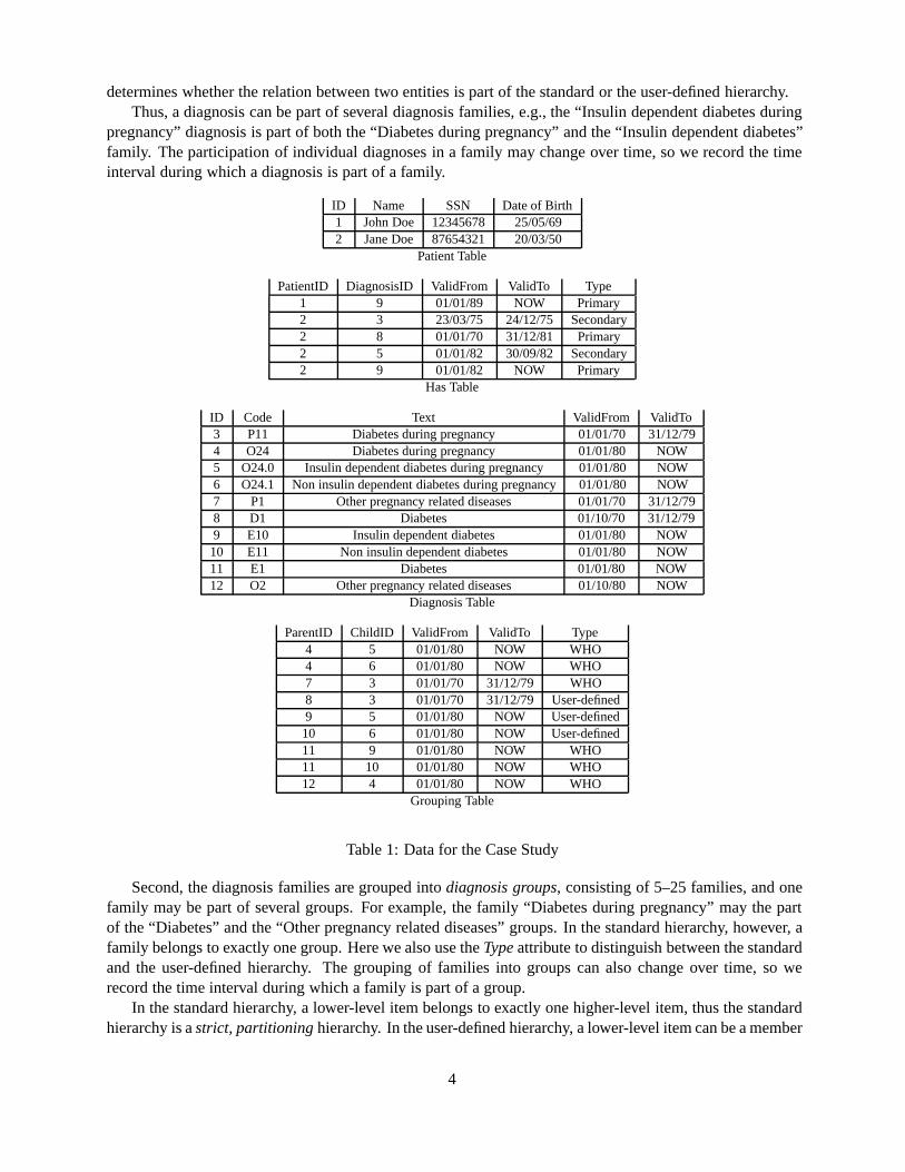
Table 1: Data for the Case Study

Second, the diagnosis families are grouped intodiagnosis groups, consisting of 5–25 families, and onefamily may be part of several groups. For example, the family “Diabetes during pregnancy” may the partof the “Diabetes” and the “Other pregnancy related diseases” groups. In the standard hierarchy, however, afamily belongs to exactly one group. Here we also use theTypeattribute to distinguish between the standardand the user-defined hierarchy. The grouping of families into groups can also change over time, so werecord the time interval during which a family is part of a group.

In the standard hierarchy, a lower-level item belongs to exactly one higher-level item, thus the standardhierarchy is astrict, partitioninghierarchy. In the user-defined hierarchy, a lower-level item can be a member

4

of zero or more higher-level items, making it anon-strict, non-partitioninghierarchy. Properties of thehierarchies will be discussed in more detail in Section 3.4.

We also record the place of residence for the patients. A patient may only live in one place at any onepoint in time. When people move, their previous address is still interesting, so we also record the associatedperiod of residence. We record the place of residence at the granularity of anarea, which designates asmall, bounded area of a few square kilometers. An area is part of exactly onecounty, which in turn is partof exactly oneregion. Thus, we have astrict, partitioning hierarchy. For areas, counties, and regions wejust record the name.

In order to list some example data, we assume a standard mapping of the ER diagram to relationaltables, i.e., one table per entity type, one-to-many relationships handled using foreign keys, and many-to-many relationships handled using separate tables. Relationships that change over time are also handledusing separate tables. We also assume the use of surrogate keys, namedID, with globally unique values.Dates are written in the format dd/mm/yy. For theValid Toattribute, we use the special value “NOW” valuethat denotes the current time2 [25]. As the three subtypes of the Diagnosis type do not have any attributes oftheir own, all three are mapped to a common Diagnosis table. The “is part of” and “grouping” relationshipsare also mapped to a common “Grouping” table. The data consists of two patients, four diagnostizations,and 10 diagnoses in a hierarchy. On January 1, 1980, a new, more detailed classification with a new codingscheme is introduced. The resulting tables are shown in Table 1 and will be used in examples throughoutthe paper.

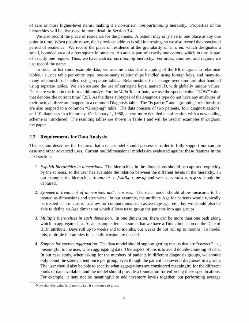
2.2 Requirements for Data Analysis

This section describes the features that a data model should possess in order to fully support our samplecase and other advanced uses. Current multidimensional models are evaluated against these features in thenext section.

1. Explicit hierarchies in dimensions. The hierarchies in the dimensions should be captured explicitlyby the schema, so the user has available the relation between the different levels in the hierarchy. Inour example, the hierarchiesdiagnosis � family � group andarea � county � region should becaptured.

2. Symmetric treatment of dimensions and measures. The data model should allow measures to betreated as dimensions and vice versa. In our example, the attribute Age for patients would typicallybe treated as a measure, to allow for computations such as average age, etc., but we should also beable to define an Age dimension which allows us to group the patients into age groups.

3. Multiple hierarchies in each dimension. In one dimension, there can be more than one path alongwhich to aggregate data. As an example, let us assume that we have a Time dimension on the Date ofBirth attribute. Days roll up to weeks and to months, but weeks do not roll up to months. To modelthis, multiple hierarchies in each dimension are needed.

4. Support for correct aggregation. The data model should support getting results that are “correct,” i.e.,meaningful to the user, when aggregating data. One aspect of this is to avoid double-counting of data.In our case study, when asking for the numbers of patients in different diagnosis groups, we shouldonly count the same patient once per group, even though the patient has several diagnoses in a group.The user should also be able to specify what aggregations are considered meaningful for the differentkinds of data available, and the model should provide a foundation for enforcing these specifications.For example, it may not be meaningful to add inventory levels together, but performing average

2Note that this value isdynamic, i.e., it continues to grow.

5

calculations on them does make sense. In the field of statistical databases, a closely related conceptis summarizability[7, 8], which means that an aggregate result, e.g., total sales, can be computed bydirectly combining results from lower-level aggregations, e.g., the sales for each store.

5. Non-strict hierarchies. The hierarchies in a dimension are not always strict, i.e., we can have many-to-many relationships between the different levels in a dimension. In our example, the diagnosishierarchy is not strict. The data model should be able to handle these just as well as “ordinary” strictdimensions.

6. Many-to-many relationships between facts and dimensions. The relationship between fact and dimen-sion is not always the classical many-to-one mapping. In our case study, the same patient may haveseveral diagnoses, even at the same point in time.

7. Handling change and time. Data change over time, but we should be able to get meaningful analysisresults across changes. In the example, one diagnosis can be superseded by two new ones, but patientsare still diagnostizised with the old one. It should be possible to easily combine data across changes.The problem typically referred to as handlingslowly changing dimensions[4, 20] is part of thisproblem.

8. Handling uncertainty. In our case study, one diagnosis is superseded by two new ones. We knowthat in 90% of the cases where we used the old diagnosis, we will now use the first of the newdiagnoses. Thus, when requesting data grouped by diagnosis for a period that spans the change, wewant the old diagnosis to be counted together with the first new diagnosis. The data model shouldallow expressing this and also support giving some kind of indications in the query results, indicatinghow many of these “converted” diagnoses are counted in the result.

9. Handling different levels of granularity. Fact data might be registered at different granularities. Inour example, the diagnosis of a diabetes patient may be registered differently by different physicians.Some will use a very specific diagnosis such as “Insulin dependent diabetes,” while others will usethe more imprecise “Diabetes,” which covers several lower-level diagnoses. It should still be possibleto get correct analysis results when data is registered at different granularities.

2.3 Related Work

In this section we evaluate data models that have previously been proposed for data warehousing accordingto the requirements in the previous section.

We consider the models of Rafanelli & Shoshani [7], Agrawal et al. [6], Gray et al. [3], Kimball [4],Li & Wang [11], Gyssens & Lakshmanan [10], Datta & Thomas [14], and Lehner [12]. The models can bedivided into three groups:simple cube models, structured cube models, andstatistical objects.

The simple cube models [3, 4, 10, 14] treat data as n-dimensional cubes. Generally, the data is dividedinto facts, or measures, e.g., Age, on which calculations should be performed, anddimensions, e.g., Di-agnosis, which characterize the facts. Each dimension has a number of attributes, which can be used forselection and grouping. In our example, a “Residence” dimension having the attributes “Area,” “County,”and “Region” would be used to characterize the patients. The hierarchy between the attributes is not cap-tured explicitly by the schema of the simple cubes, so the user will not be able to learn from the schemathat Area rolls up to County and not the other way around. Star schema designs [4] are also considered as asimple cubes, as they are semantically equivalent to these.

The structured cube models [6, 11, 12] capture the hierarchies in the dimensions explicitly, providingbetter guidance for the user navigating the cubes. This information may also be useful for query optimization

6

[15]. The hierarchies are captured using eithergrouping relations[11], dimension merging functions[6], oran explicit tree-structured hierarchy as part of the cube [12].

The last group of models is thestatistical objects[7]. For this group, a structured classification hierarchyis coupled with an explicit aggregation function on a single measure to produce a “pre-cooked” object thatwill answer a very specific set of questions. This approach is not as flexible as the others, but unlike mostof these, it provides some protection (summarizability) against getting incorrect results from queries.

The results of evaluating the eight data models against our nine requirements are seen in Table 2. If amodel supports all aspects of a requirement, we say that the model providesfull support, denoted by “

p”.

If a model supports some, but not all, aspects of a requirement, we say that it providespartial support,denoted by “p”. When it is not possible for the authors to determine how support for a requirement shouldbe accomplished in the model, we say that the model providesno support, denoted by “-”.

1 2 3 4 5 6 7 8 9Rafanelli & Shoshani [7]

p- -

pp - - - -

Agrawal et al. [6] pp p

- p - - - -Gray et al. [3] -

p pp - - - - -

Kimball [4] - -p

p - - p - -Li & Wang [11] p -

pp - - - - -

Gyssens & Lakshmanan [10] -p p

p - - - - -Datta & Thomas [14] -

p p- p - - - -

Lehner [12]p

- -p

- - - - -

Table 2: Evaluation of the Data Models

1. Explicit hierarchies in dimensions: The simple cube models [3, 4, 10, 14] do not capture the hierar-chies in the dimensions explicitly. Some models provide partial support by thegrouping relation[11]anddimension merging function[6] constructs, but do not capture the complete hierarchy togetherwith the cube. This is done by the last two models [7, 12], thus capturing the full cube navigationsemantics in the schema.

2. Symmetric treatment of dimensions and measures: Half of the models [4, 7, 11, 12] distinguish sharplybetween measures and dimensions. An attribute designated as a measure cannot be used as a dimen-sional attribute and vice versa. This restricts the flexibility of the cube designs, e.g., if the Ageattribute of the example is a measure, it cannot be used to group patients into age groups. The otherhalf of the models [3, 6, 10, 14] do not impose this restriction. They either do not distinguish betweenmeasures and dimensions [3, 10], or they allow for the conversion of measures to dimensions andvice versa [6, 14].

3. Multiple hierarchies in each dimension: Some models [7, 12] require that the dimension hierarchiesare tree-structured. To support multiple hierarchies, a more general lattice structure is required. Allthe other models [3, 4, 6, 10, 11, 14] allow multiple hierarchies.

4. Support for correct aggregation: Half of the models [3, 4, 10, 11] support correct aggregation par-tially, by implicitly requiring the dimension hierarchies to bestrict andpartitioning, i.e., a lower-levelitem maps to exactly one item on the next level. This is one of the conditions of summarizability [8].Two of the models allow for non-strict hierarchies, while not addressing the issue of double-counting,thus providing no support [6, 14]. The remaining two models [7, 12] place explicit conditions on both

7

the hierarchy (strict and partitioning) and the aggregation functions used (only additive data may beadded, etc.), thus providing full support for correct aggregation.

5. Non-strict hierarchies: Most of the models [3, 4, 10, 11, 12] implicitly or explicitly require thathierarchies be strict. Two models [6, 14] mention briefly that non-strict hierarchies are allowed, butdoes not go deeper into the issues raised by allowing this, e.g., the possibility of double-counting andthe use of pre-computed aggregates. The remaining model [7] investigates the possible problems withallowing non-strict hierarchies and advises against using this feature.

6. Many-to-many relationships between facts and dimensions: None of the models allow many-to-manyrelationships between facts and their associated dimensions, such as the relationship between patientsand diagnoses in the example.

7. Handling change and time: Only one model [4] discusses this issue, but none the proposed solutionsfully support analysis across changes in the dimensions. None of the other models support analysisacross changes, although one mention that this is a very important issue [12].

8. Handling uncertainty: None of the models provide built-in support for uncertainty in the data.

9. Handling different levels of granularity: None of the models handle different levels of granularity inthe data.

To conclude, the models generally provide full or partial support for most of requirements 1–4. Require-ment 5 (non-strict hierarchies) is partially supported by three of the models, while requirement 7 (handlingchange and time) is only partially supported by Kimball [4]. Requirements 6, 8, and 9 are not supported byany of the models. The objective of the model proposed in this paper is to support all nine requirements.

3 An Extended Multidimensional Data Model

In this section we define our model. For every part of the model, we define theintension, the extension,and give an illustrating example. To avoid unnecessary complexity, we first define the basic model and thendefine extensions for handling time and uncertainty later.

3.1 The Basic Model

An n-dimensional fact schemais a two-tupleS � �F �D�, whereF is afact typeandD � fTi� i � �� ngis its correspondingdimension types.

Example 1 In the case study from Section 2.1 we will havePatientas the fact type, andDiagnosis, Res-idence, Age, Date of Birth (DOB), Name, andSocial Security Number (SSN)as the dimension types. Theintuition is thateverythingthat characterizes the fact type is considered to bedimensional, even attributesthat would be considered asmeasuresin other models.

A dimension typeT is a four-tuple�C��T ��T ��T �, whereC � fCj � j � �� kg are thecategorytypesof T , �T is a partial order on theCj ’s, with �T � C and�T � C being the top and bottom elementof the ordering, respectively. Thus, the category types form a lattice. The intuition is that one category typeis “greater than” another category type if members of the former’s extension logically contain members ofthe latter’s extension, i.e., they have a larger element size. The top element of the ordering corresponds tothe largest possible element size, that is, there is only one element in it’s extension, logically containing allother elements.

8

We say thatCj is a category type ofT , writtenCj � T , if Cj � C. We assume a functionPred � C �� C

that gives the set of immediate predecessors of a category typeCj.

Example 2 Low-level diagnoses are contained in diagnosis families, which are contained in diagnosisgroups. Thus, theDiagnosisdimension type has the following order on its category types:�Diagnosis

= Low-level Diagnosis� Diagnosis Familiy� Diagnosis Group� �Diagnosis. We have thatPred �Low-level Diagnosis� � fDiagnosis Familyg. Other examples of category types areAgeandTen-year Age Groupfrom the Age dimension type, andDOBandYearfrom the DOB dimension type. Figure 2, to be discussedin detail later, illustrates the dimension types of the case study.

Many types of data, e.g., ages or sales amounts, can be added together to produce meaningful results.This data has an ordering on it, so computing the average, minimum, and maximum values make sense. Forother types of data, e.g., dates of birth or inventory levels, the user may not find it meaningful in the givencontext to add them together. However, the data has an ordering on it, so taking the average, or computingthe maximum or minimum values do make sense. Some types of data, e.g., diagnoses, do not have anordering on them, and so it does not make sense to compute the average, etc. Instead, the only meaningfulaggregation is to count the number of occurrences.

We can support correct aggregation of data by keeping track of what types of aggregate functions canbe applied to what data. This information can then be used to either prevent users from doing “illegal”calculations on the data completely, or to warn the users that the result might be “wrong,” e.g., the samepatient is counted twice, etc. In line with this reasoning and previous work [12, 19], we distinguish betweenthree types of aggregate functions:�, applicable to data that can be added together,�, applicable to data thatcan be used for average calculations, andc, applicable to data that is constant, i.e., it can only be counted.Considering only the standard SQL aggregation functions, we have that� � fSUM, COUNT, AVG, MIN,MAX g, � � fCOUNT, AVG, MIN, MAXg, and c � fCOUNTg. The aggregation types are ordered,c � � � �, so data with a higher aggregation type, e.g.,�, also possess the characteristics of the loweraggregation types. For each dimension typeT � �C��T �, we assume a functionAggtypeT � C �� f�� cgthat gives the aggregation type for each category type.

Example 3 In the case study,Aggtype�Low-level Diagnosis� � c, Aggtype�Age� � �, Aggtype�Ten-yearAge Group� � c, andAggtype�DOB� � �.

A dimensionD of typeT � �fCjg��T ��T ��T � is a two-tupleD � �C��, whereC � fCjg is aset ofcategoriesCj such thatType�Cj� � Cj and� is a partial order on�jCj , the union of all dimensionvalues in the individual categories. A categoryCj of type Cj is a set ofdimension valuese such thatType�e� � Cj.

The definition of the partial order is: given two valuese�� e� thene� � e� if e� is logically contained ine�. We say thatCj is a category ofD, writtenCj � D, if Cj � C. For a dimension valuee, we say thate isa dimensional value ofD, writtene � D, if e � �jCj .

The category type�T in dimension typeT contains the values with the smallest value size. Thecategory type with the largest value size,�T , contains exactly one value, denoted�. For all valuese of thecategory types ofD, e � �. Value� is similar to theALL construct of Gray et al. [3].

Example 4 In our Diagnosisdimension we have the following categories, named by their type.Low-levelDiagnosis= f�� g, Diagnosis Family= f� �� g, Diagnosis Group= f�� g, and�Diagnosis �f�g. The values in the sets refer to theID field in the Diagnosis table of Table 1. The partial order� isgiven by the first two columns in the Grouping table in Table 1. Additionally, the top value� is greaterthan, i.e., logically contains, all the other diagnosis values.

9

We say that the dimensionD� � �C �� is asubdimensionof the dimensionD � �C�� if C� C

ande� �� e� �C�� C� � C ��e� � C�� e� � C� � e� � e�� , that is,D� has a subset of the categories ofD and�� is the restriction of� to these categories. We note thatD is a subdimension of itself.

Example 5 We obtain a subdimension of the Diagnosis dimension from the previous example by removingtheLow-level DiagnosisandDiagnosis Familycategories, retaining onlyDiagnosis Groupand�Diagnosis .

It is desirable to distinguish between the dimension values in themselves and the real-world “names”that we use for them. The names might change or the same value might have more than one name, makingthe name a bad choice for identifying an value. In common database terms, this is the argument forobjectids or surrogates.

To support this feature, we require that a categoryC has one or morerepresentations. A representationRep is a bijective functionRep � Dom�C� DomRep, i.e., a value of a representation uniquely identifiesa single value of a category and vice versa, thus making the representation an “alternate key.” We use thenotationRep�e� � v to denote the mapping from dimension values to representation values.

Example 6 A diagnosis value has two representations,CodeandText. Using the ID’s from the Diagnosistable to identify the values, we haveCode�� O�� andText�� Diabetes during pregnancy��

Let F be a set of facts, andD � �fCjg�� a dimension. Afact-dimension relationbetweenF andD is a setR � f�f� e�g, wheref � F ande � �jCj. ThusR links facts to dimension values. We saythat factf is characterized bydimension valuee, written f � e, if �e� � D ��f� e�� R � e� � e�.We require that�f � F ��e � �jCj ��f� e� � R��; thus we do not allow missing values. The reasons fordisallowing missing values are that they complicate the model and often have an unclear meaning. If it isunknown which dimension value a factf is characterized by, we add the pair�f�� to R, thus indicatingthat we cannot characterizef within the particular dimension.

Example 7 The fact-dimension relationR links patient facts to diagnosis dimension values as given by theHas table from the case study. Leaving out the temporal aspects for now, we get thatR � f(1,9), (2,3),(2,5), (2,8), (2,9)g. Note that we can relate facts to values in higher-level categories, e.g., fact 1 is relatedto diagnosis 9, which belongs to theDiagnosis Familycategory. Thus, we do not require thate belongs to�Diagnosis , as do the existing data models. If no diagnosis is known for patient 1, we would have added thepair �� toR.

A multidimensional object(MO) is a four-tupleM � �S� F�D�R�, whereS � �F �D � fTig� isthe fact schema,F � ffg is a set offacts f whereType�f� � F , D � fDi� i � �� ng is a set ofdimensionswhereType�Di� � Ti, andR � fRi� i � �� ng is a set of fact-dimension relations, such that�i��f� e� � Ri � f � F � �Cj � Di�e � Cj��.

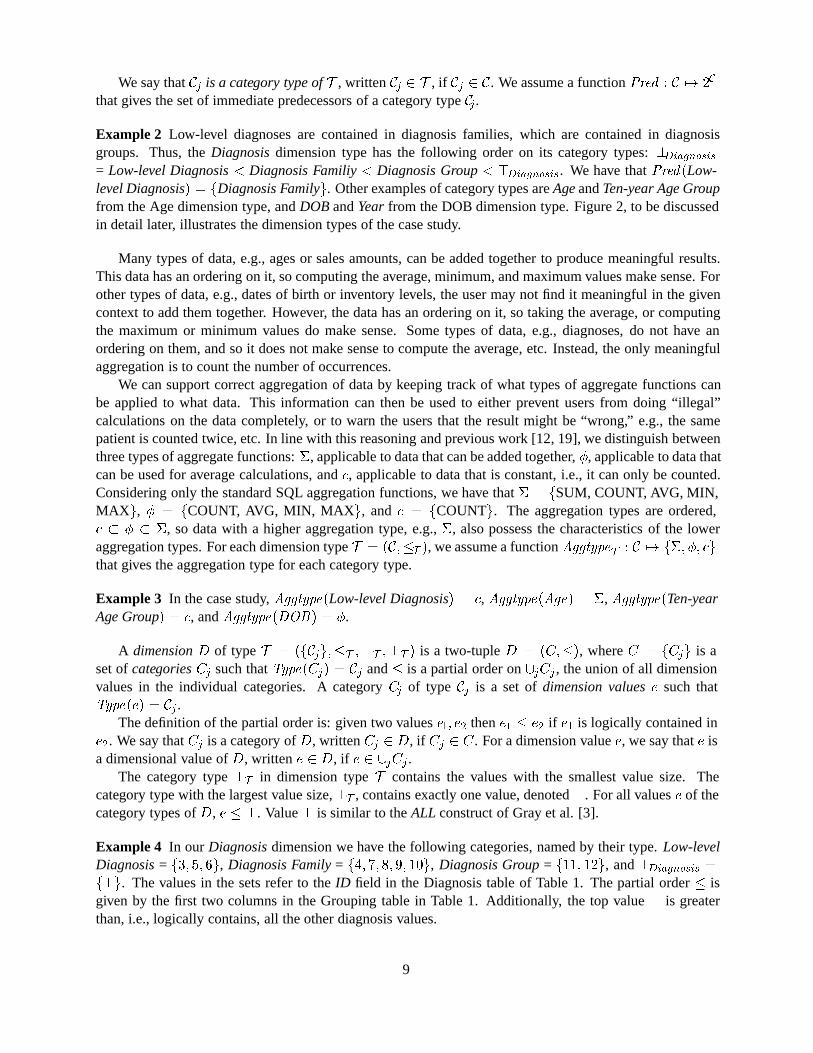
Example 8 For the case study, we get a six-dimensional MOM � �S� F�D�R�, whereS � �Patient,fDiagnosis, DOB, Residence, Name, SSN, Ageg� andF � f�� g. The definition of the diagnosis di-mension and its corresponding fact-dimension relation was given in the previous examples. Due to spaceconstraints, we do not list the contents of the other dimensions and fact-dimension relations, but just outlinetheir structure. The Name and SSN dimensions are simple, i.e., they just have a� category type, Namerespectively SSN, and a� category type. The Age dimension groups ages (in years) into five-year andten-year groups, e.g., 10–14 and 10–19. The Date-of-Birth dimension has two hierarchies in it: days aregrouped into weeks, or days are grouped into months, with the further levels of quarters, years, and decades.We will refer to this MO as the “Patient” MO. A graphical illustration of the schema of the “Patient” MO isseen in Figure 2.

10

Day =

Week Month

Quarter

Year

⊥

⊥Low-level Diagnosis = ⊥

Diagnosis Family

Diagnosis Group

⊥

DiagnosisDimension

Date of BirthDimension

ResidenceDimension

Area = ⊥

County

Region

⊥

Patient

Decade

Name = ⊥

⊥

NameDimension

SSNDimension

⊥

SSN= ⊥Age = ⊥

Five year group

Ten year group

⊥

AgeDimension

Figure 2: Schema of the Case Study.

A collection of multidimensional objects, possibly with shared subdimensions, is called amultidimen-sional object family.

Example 9 To illustrate the usefulness of shared subdimensions in multidimensional object families, imag-ine performing the following steps. Create a subdimension of the Diagnosis dimension that includes onlyDiagnosis Groupand�Diagnosis, and a subdimension of the Age dimension that includes onlyTen-YearGroup and�Age. Make an MO with these two dimensions and the fact type Patient for all patients in thecountry. This results in an MO capturing all patients in the country together with their diagnosis groupsand their ten-year age groups. Putting this MO together with the “Patient” MO from the example above, weobtain a multidimensional object family with two shared subdimensions. The shared subdimensions couldbe used to investigate how diagnoses versus age groups for the patient group from the case study compareto the national average.

To summarize the essence of our model, the facts are objects with aseparate identity. Thus, we can testfacts for equality, but we do not assume an ordering on the facts. The combination of dimensions valuesthat characterize the facts of a fact set isnot a “key” for the fact set. Thus, we may have “duplicate values,”in the sense that several facts may be characterized by the same combination of dimension values. But, thefacts of an MO is aset, so we do not have duplicatefactsin an MO.

3.2 Handling Time

We now investigate how to build temporal support into the model. The vast majority of research in temporaldata models assumes a discrete time domain (for example, most data models in the most recent collectionof temporal database papers [16] explicitly assume a discrete model of time). Also the temporal data typesoffered by the SQL standard [17] are discrete and bounded. Thus, we assume a time domain that is discreteand bounded, i.e., isomorphic with a bounded subset of the natural numbers. The values of the time domainare calledchronons. They correspond to the finest granularity in the time domain [22]. We letT , possiblysubscripted, denote a set of chronons.

11

Thevalid timeof a statement is the time when the statement is true in the modeled reality [1]. Valid timeis very important to capture because the real world is where the users reside, and weallow the attachmentof valid time to the data, but do not require it. If valid time is not attached to the data, we assume the datato bealwaysvalid. If valid time is attached to an MO, we call it avalid-timeMO.

In general, valid time may be assigned to anything that has a truth value. In our model, this is the par-tial order between dimension values, the mapping between values and representations, the fact-dimensionrelations, and the membership of values in categories. It is important to be able to capture all these aspects.

We add valid time to the dimension partial order� by addingTv, the set of chronons during which therelation holds in the real world, to each relation between two values. We write thate� �Tv e� if e� � e�during each chronon inTv. The partial order�Tv has the following property:e� �T�v e� � e� �T�v e� �e� �T�v�T�v e�. Similarly, we writeRep�e� �Tv v to denote that the representationRep of the valuee hasvaluev during each chronon inTv. For each fact-dimension relation between a factf and a dimension valuee, we capture the set of chrononsTv when the two are related. We write�f� e� �Tv R when�f� e� � R

during each chronon inTv. We use the notationf �Tv e when �f� e�� Tv R � e� �Tv e. Finally, weadd valid time to membership of dimension values in categories, writinge �Tv C whene � C during eachchronon inTv.

The set of chronons that is attached to a statement is themaximalset of chronons when the statementis valid, so the data is always “coalesced” [1]. Thus, we do not have the problem of “value-equivalent”statements [1, 21, 23], where the same statement appears several times with different times attached to it,e.g.,e� �T� e� ande� �T� e�, whereT� �� T�. However, by implication, statements are valid for any subsetof their attached time, e.g.,T� T� � e� �T� e� � e� �T� e�.

Example 10 For our examples, we use interval notation forTv, with the chronon size equal to Day. For thepartial order for the Diagnosis dimension, we have� �� . For the representation, we haveCode�� D�. For the fact-dimension relation, we have�� R.For the category membership, we have�� NOW � Diagnosis Family.

To sum up, by extending the dimension partial order with links between dimension values that representthe “same” thing across change, we have a foundation for handling analysis across changes. This allows usto obtain meaningful results when we analyze data across changes in the dimension.

Example 11 When looking at the data from the current point in time, we want to count the patients diag-nosed with the old “Diabetes” diagnosis�ID � �� together with those diagnoses with the new “Diabetes”diagnosis�ID � �� when we look at diagnostizations from 1970 to the present. This is done by definingthat� ��NOW � ��, i.e., from 1980 up till now, we consider the diagnosis 8 to be logically containedin the diagnosis 11.

Valid time is not the only temporal aspects that may be interesting to our model. It is also interestingto capture when statements are present in the database, as the time a statement is present in the databasealmost never corresponds to the time it is true in the real world. We need to know when data are present inthe database for accountability and traceability purposes.

Thetransaction timeof a statement is the time when the statement is current in the database and may beretrieved [1]. Generally, transaction time can be attached to anything that valid time can be attached to. Theaddition of transaction time is orthogonal to the addition of valid time. Additionally, transaction time canbe added to data that does not have a truth value. In our model, we could record when facts, e.g., patients,are present in the database. We do not think that this is very interesting in itself, as facts are only interestingwhen they participate in fact-dimension relations. Thus, we do not record this.

If transaction time is attached to an MO, we call it atransaction-timeMO. If both valid and transactiontime is attached to an MO, we call it abitemporalMO. If no time is attached to an MO, we call it asnapshot

12

MO. In our notation, we useTt to denote the set of chronons when data is current in the database. We useTt � Tv to denote sets of bitemporal chronons.

3.3 Handling Uncertainty

Sometimes the data available contains uncertainties that cannot adequately be captured using standard tech-niques such as default values, etc. Instead, we handle this uncertainty explicitly in our data model. To do so,we introduce measures of probability. In general, it makes sense to attach a probability to a statement if thestatement can be given a valid time. In our model, this applies to dimension partial orders, fact-dimensionrelations, mappings between values and representations, and category memberships for values. However,we attach probabilities to the former two only. It is of little use to have a probability for the mapping be-tween values and representations, which would violate the requirement that a representation is an alternatekey. Also, giving probabilities to the membership of categories is omitted, as values belong fully to onecategory at any given time.

First, we add probability to the partial order on dimension values. Given two dimension valuese�� e�and a numberp such that� � p � �, we write thate� �p e� if e� � e� with probability p. Second,we add probability to a fact-dimension relationR. Given a factf , a dimension valuee and a numberpsuch that� � p � �, we write that�f� e� �p R if �f� e� � R with probability p. We writef �p e if�f� e�� p� R � e� �p� e � p � p� � p�. Note that a probability is assigned toall (ancestor,descendent) linksin the partial order, not just the direct (parent,child) links.

Example 12 Before 1980, diagnostizations in the case study do not differentiate between insulin dependentand non insulin dependent diabetes. From 1980 and on this is the case. Suppose that we know that 90%of the diagnostizations made with the old “Diabetes” diagnosis were for insulin dependent diabetes cases.When looking for the number of insulin dependent diabetes patients from 1970 up till now, we want tocount the old “Diabetes” diagnostizations too. We do this by extending the Diagnosis partial order with theinformation that� �� .

Suppose that physicians are allowed to express their belief in the correctness of a diagnostization byattaching a probabilityp to it. In the case study, the physician is 95% certain that John Doe�ID � �� hasinsulin dependent diabetes�ID � �. Thus, for the fact-dimension relation R,�� R.

To summarize, the addition of uncertainty to the model is orthogonal to the features for handling time,thus any combination of extensions is valid. If both time and probabilities are added to an MO, we assigna probabilitypt for eachchronont in the chronon setT . This is done to avoid the problems of value-equivalent tuples. However, interval notation such as� ��NOW � is used in examples. If probabilityis assigned to an MO, we call it aprobabilistic MO. If no probability is assigned, we call it adeterministicMO.

3.4 Properties of the Model

In this section important properties of the model that relate to the use of pre-computed aggregates is definedand discussed. The first important concept issummarizability, which intuitively means that individualaggregate results can be combined directly to produce new aggregate results.

Definition 1 Given a typeT , a setS � fSj � j � �� kg, whereSj � �T , and a functiong � �T �� T , wesay thatg is summarizablefor S if g�fg�S�� g�Sk�g� � g�S� � ��Sk�. The set of arguments on the leftside of the equation is a multi-set, or bag, i.e., the same result value can occur multiple times.

13

Summarizability is an important concept as it is a condition for the flexible use of pre-computed aggre-gates. Without summarizability, lower-level results generally cannot be directly combined into higher-levelresults. This means that we cannot choose to pre-compute only a relevant selection of the possible aggre-gates and then use these to compute higher-level aggregates on-the-fly. Instead, we have to pre-compute thetotal results for all the aggregations that we need fast answers to, while other aggregates must be computedfrom the base data. Space and time constraints can be prohibitive for pre-computing all results, while com-puting aggregates from scratch results in long response times. In this case, an attractive alternative is theuse ofsamplingtechniques to answer the queries [24]. Using sampling, only a small sample of the availabledata is read and used toestimatethe result of the query. This can produce very fast response times, whilemaintaining a relatively high degree of accuracy for the result.

It has been shown that summarizability is equivalent to the aggregation function beingdistributive, allpaths beingstrict, and the hierarchies beingpartitioning in the relevant dimensions [8]. If data with timeattached to it is aggregated such that data for one fact is only counted for one point in time, this result extendsto hierarchies that aresnapshot strictandsnapshot partitioning. These concepts are formally defined below.In the definitions, we assume a dimensionD � �C��.

Definition 2 If �C�� C� � C�e�� e� � C� � e� � C� � e� � e� � e� � e� � e� � e�� then the mappingbetweenC� andC� is strict. Otherwise, it isnon-strict. The hierarchy in dimensionD is strict if allmappings in it are strict; otherwise, it isnon-strict. Given a categoryCj � Di, we say that there is astrictpath from the set of factsF to Cj iff �f � F � f � e� � f � e� � e� � Cj � e� � Cj � e� � e�

3. Thehierarchy in dimensionD is snapshot strict, if at any given timet, the hierarchy is strict.

Definition 3 If �C� � C�C� �� D � e� � C� � �C� � Pred �C��e� � C��e� � e��, i.e., if everynon-top value has a direct parent, we say that the hierarchy in dimensionD is partitioning; otherwise, it isnon-partitioning. The hierarchy in dimensionD is snapshot partitioningif at any given timet, the hierarchyis partitioning.

Example 13 The hierarchy in the Residence dimension is strict and partitioning. The hierarchy in the Di-agnosis dimension is non-strict and partitioning, but could have been non-partitioning. The sub-hierarchy ofthe Diagnosis dimension obtained by restriction to the standard classification is snapshot strict and snapshotpartitioning.

4 The Algebra

This section defines an algebra on the multidimensional objects just defined. In line with the model defi-nition, we first define the basic algebra and then define extensions for handling time and uncertainty. Forsome of the more complex operators, we provide examples of their use.

4.1 The Basic Algebra

We first define the fundamental operators. These are close to the standard relational algebra operators.For unary resp. binary operators, we assume a multidimensional objectM � �S� F�D � fDig� R �fRig�� i � �� n and multidimensional objectsMk � �Sk� Fk� Dk � fDkikg� Rk � fRkik

g�� k � �� .We note that the representations of the categories in the resulting MO’s are the same as in the argumentMO’s, thus we do not specify the values representations for the resulting MO’s. The aggregation types areonly changed by the aggregate formation operator, so they are not specified for the other operators.

3Note that the paths from the set of factsF to the�T categories are always strict.

14

For the operator definitions, we need some preliminary definitions. First, we defineGroup, that groupsthe facts characterized by the same dimension values together. Given an n-dimensional MO,M � �S� F�D �fDig� R � fRig�� i � �� n, a set of categoriesC � fCi j Ci � Dig� i � �� n, one from eachof the dimensions ofM , and an n-tuple�e�� en�, whereei � Ci� i � �� n, we defineGroup as:Group�e�� en� � ff j f � F � f �� e� � �� f �n eng.

Next, we define aunionoperator on dimensions, which performs union on the categories and the partialorders. Given two dimensionsD� � �C�� andD� � �C�� of type T , whereCk � fCkjg� k �� j � �� m, we define the union operator on dimensions,

SD, as: D�

SDD� � �C ��, where

C � � fC �jg� j � �� m, C �

j � C�j � C�j, where� denotes regular set union, ande� �� e� e� ��

e� � e� �� e�.

selection: Given a predicatep on the dimension typesD � fTig, we define the selection� as:��p��M� ��S �� F �� D�� R��, whereS � � S, F � � ff � F j �e� � D�� en � Dn � p�e�� en��f �� e�� f �n

en�g, D� � D, R� � fR�ig, andR�

i � f�f �� e� � Ri j f � � F �g. Thus, we restrict the set of facts tothose that are characterized by values wherep evaluates to true. The fact-dimension relations are restrictedaccordingly, while the dimensions and the schema stay the same.

Example 14 If selection is applied to the “Patient” MO with the predicateName �”John Doe,” the result-ing MO has the same schema, the factsF� � f�g, the fact-dimension relationsR�i � f�� e� j �� e� � Rig,e.g.,R� � f�� g, and the dimensionD� � D.

projection: Without loss of generality, we assume that the projection is over thek dimensionsD�� Dk.We then define the projection� as: ��D�� Dk��M� � �S �� F �� D�� R��, whereS � � �F ��D�� F � �F � D� � fT�� Tkg� F � � F� D� � fD�� Dkg, andR� � fR�� Rkg. Thus, we retain only thekdimensions, but the set of facts stays the same. Note that we do not remove “duplicate values.” Thus thesame combination of dimension values may be associated with several facts.

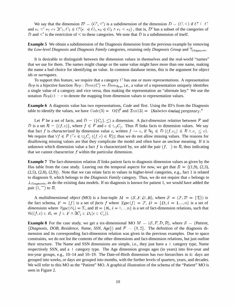
Example 15 If projection over the Name and Diagnosis dimensions is applied to the “Patient” MO, theresulting MO has the same fact type, only the Name and Diagnosis dimension types, the same set of facts,the Name and Diagnosis dimensions, and the fact-dimension relations for these two dimensions. A graphicalillustration of the resulting MO is seen to the left in Figure 3.

1 2

JohnDoe

JaneDoe

⊥

Namedimension

7 8 4 9 10

3 5 6

12 11

⊥

Diagnosisdimension

DiagnosisGroup

DiagnosisFamily

Low-levelDiagnosis

Name

Patient{1,2}{2}

12 11

⊥

Diagnosisdimension

Result dimension

⊥

1 20...

0-1 >1

Set-of-Patient

DiagnosisGroup Count

Range

Figure 3: Resulting MO’s for Projection and Aggregate Formation

15

rename: Given a multidimensional object,M � �S� F�D�R�, and fact schemaS� � �F ��D��, such thatD is isomorphic withD�, we define the rename� as:��S��M� = M �, whereM � � �S �� F�D�R�. We seethat rename just return the contents ofM with the new schemaS�, which has the same structure as the oldschemaS. Rename is used to alter the names of dimensions so that dimensions with the same name, e.g.,resulting from a “self-join,” can be distinguished.

union: Given two n-dimensional MO’s,Mk � �Sk� Fk�Dk� Rk�� k � �� such thatS� � S�, we definethe union

Sas: M�

SM� � �S �� F ��D�� R��, whereS � � S�� F

� � F� � F�� D� � fD�i

SDD�i � i �

�� ng� andR� � fR�i �R�i � i � �� ng. In words, given two MO’s with common schemas, we take theset union of the facts and the fact-dimension relations. The

SD operator is used to combine the dimensions.

difference: Given two n-dimensional MO’s ,Mk � �Sk� Fk�Dk� Rk�� k � �� such thatS� � S�, wedefine the differencen as: M� n M� � �S �� F ��D�� R��, whereS � � S�� F

� � F� n F�� D� � D�,R� � fR�

i� i � �� ng, with R�i � f�f �� e� j f � � F � � �f �� e� � R�i . Thus, given two MO’s with common

schemas, we take the set difference of the facts, the dimensions of the first argument MO are retained, andthe fact-dimension relations are restricted to the new fact set. Note that we do not take the set difference ofthe dimensions, as this does not make sense.

Example 16 Performing the difference operator on the MO resulting from the projection example and theMO resulting from applying the selectionName � ��Jane Doe�� to the projection MO gives as a result anMO with the same schema, with the fact setF � f�g, the dimensions from the first argument, and thefact-dimension relationsR� � f�� g andR� � f�� John Doe�g.

identity-based join: Given two MO’s,M� andM�, and a predicatep�f�� f�� ff� � f�� f� �� f�� trueg,we define the identity-based join� as: M� ��p� M� � �S �� F ��D�� R��, where�S � � �F ��D��, F � �F� � F�, D� � D� � D�, F � � f�f�� f�� j f� � F� � f� � F� � p�f�� f��g, D� � D� � D�,R� � fR�

i� i � �� n��n�g, andR�i � f�f �� e�jf � � �f�� f�� f � � F � � ��i � n�� f�� e� � R�i�� i �

n� � �f�� e� � R�i�n��g. In words, the new fact type is the type ofpairs of the old fact types, and the new

set of dimension types is the union of the old sets. The set of facts is the subset of the cross product of theold sets of facts where the join predicatep holds. Forp equal tof� � f�, f� �� f�, andtrue, the operationis anequi-join, non-equi-join, andCartesian product, respectively. For the instance, the set of dimensionsis the set union of the old sets of dimensions, and the fact-dimension relations relates a pair to an value ifone member of the pair was related to that value before.

Example 17 We want to know if any patients are registered with more than one name. We take two copiesof the “Patient” MO and perform projection over the Name dimension for both. For the second copy, theName dimension type is renamed to “Name2”. We then perform an identity-based join of the two with thepredicatef� � f�. This gives us an MO with two dimension types,NameandName2. The fact type isthe type of pairs of patients; the set of facts is stillF � f�� g, and the contents of the two dimensionsare identical. The fact-dimension relations are also identical:R� � f�� John Doe�� Jane Doe�g andR� � f�� John Doe�� Jane Doe�g. We can now perform a selection on this MO with the predicateName�� Name2to find patients with more than one name.

aggregate formation: The aggregate formation operator is used to compute aggregate functions on theMO’s. For notational convenience and following Klug [18], we assume the existence of afamily of aggre-gation functionsg that take somek-dimensional subsetfDi� � �� Dikg of then dimensions as arguments,e.g.,SUM i sums thei-th dimension andSUMij sums thei-th andj-th dimensions. We assume a functionArgs�g� � fj j g uses dimensionj as argumentg that returns the argument dimensions ofg.

16

Given an n-dimensional MO,M , a dimensionDn�� of typeTn��, a function,g � �F �� Dn��4 such that

g � MIN fAggtype��Dij�� j � Args�g�g, and a set of categoriesCi � Di� i � �� n, we define aggregate

formation,�, as: ��Dn�� g� C�� Cn��M� � �S �� F ��D�� R��, whereS � � �F ��D��, F � � �F , D� �fT �

i � i � �� ng � fTn��g, T �i � �C�i��

Ti��

Ti��

Ti�, C�i � fCij � Ti j Type�Ci� �Ti Cijg, ��

Ti� �TijC�

i

,

��Ti

� Type�Ci�,��Ti

� �Ti ,F� � fGroup�e�� en� j �e�� en� � C��Cn�Group�e�� en� �� g,

D� � fD�i� i � �� ng � fDn��g, D�

i � �C �i��

i�, C�i � fC �

ij � Di j Type�C �ij� � C�ig, ��

i � �ijD�i

, R� �

fR�i� i � �� ng�fR�

n��g,R�i � f�f �� e�i� j ��e�� en� � C��Cn �f

� � Group�e�� en��f � � F ��ei � e�i�g, andR�

n�� e��en �C��Cn f�Group�e�� en�� g�Group�e�� en�� j Group�e�� en� ��g. The aggregation types for the remaining parts of the argument dimensions are not changed. Theaggregation types for the result dimension is given by the following rule. Ifg is distributive, the pathsto C�� Cn are strict, and the hierarchies up toC�� Cn are partitioning, thenAggtype��Dn�� MIN fAggtype��Dj

�� j � Args�g�g. Otherwise,Aggtype��Dn�� c. For the higher categories inthe result dimension,Aggtype�C�

m� � MIN fAggtype�Cm��Aggtype��Dn��g.Thus, for every combination�e�� en� of dimension values in the given “grouping” categories, we

apply g to the set of factsffg, where thef ’s are characterized by�e�� en�, and place the result in thenew dimensionDn��. The facts are of typesetsof the argument fact type, and the argument dimensiontypes are restricted to the category types that are greater than or equal to the types of the given “grouping”categories. The dimension type for the result is added to the set of dimension types. The new set of factsconsists of sets of facts, where the facts in a set share a combination of characterizing dimension values. Theargument dimensions are restricted to the remaining category types, and the result dimension is added. Thefact-dimension relations for the argument dimensions now link sets of facts directly to their correspondingcombination of dimension values, and the fact-dimension relation for the result dimension links sets of factsto the function results for these sets. If the functiong is distributive, the paths up to the grouping categoriesare strict, and the hierarchy up to the grouping categories is partitioning, i.e., g is “summarizable,” thenthe aggregation type for the bottom category in the result dimension is the minimum of the aggregationtypes for the bottom categories in the dimensions thatg uses as arguments ; otherwise, the aggregation typeis c. For the higher categories, the minimum of the aggregation types given in the result dimension andthe bottom category’s aggregation type is used. Thus, aggregate results that are “unsafe” in the sense thatthey contain overlapping data, cannot be used for further aggregation. This prevents the user from gettingincorrect results by accidentally “double-counting” data.

Example 18 We want to know the number of patients in each diagnosis group. To do so, we apply theaggregate-formation operator to the “Patient” MO with theDiagnosis Groupcategory and the� categoriesfrom the other dimensions. The aggregate functiong to be used isset-count, which counts the number ofmembers in a set. The resulting MO has seven dimensions, but only the Diagnosis and Result dimensionsare non-trivial, i.e., the remaining five dimensions contain only the� categories. The set of facts is stillF � f�� g. The Diagnosis dimension is cut, so that only the part fromDiagnosis Groupand up is kept.The result dimension groups the counts into two ranges: “0–1” and “�1”. The fact-dimension relation forthe Diagnosis dimension links the sets of patients to their corresponding Diagnosis Group. The contentis: R� � f�f�� g� �� f�g� ��g, meaning that the sets of patientsf�� g andf�g are characterized bydiagnosis groups�� and��, respectively. The fact-dimension relation for the result dimension relate eachgroup of patient to the count for the group. The content is:R� � f�f�� g� �� f�� g� ��g, meaning that theresults ofg on the setsf�� g andf�g are� and�, respectively. A graphical illustration of the MO, leavingout the trivial dimensions for simplicity, is seen on the right side of Figure 3. Note that each patient is onlycounted once for each diagnosis group, even though patient� hasseveraldiagnoses in each group.

4The functiong “looks up” the required data for the facts in the relevant fact-dimension relations, e.g.,SUMi finds its data infact-dimension relationRi.

17

Now, we will show how other common OLAP and relational operators can be defined in terms of thefundamental operators.

value-based join: A join of two MO’s on common dimension values can be made in the usual way bycombining Cartesian product (a special case of the identity-based join), selection, and projection.Naturaljoin is a special case of the value-based join, where the selection predicate requires that values from the“matching” dimensions should be equal, followed by projecting “out” the duplicate dimensions. Perform-ing drill-across from one MO to another is just the value-based join of the two MO’s on their commondimensions.

duplicate removal: We can remove “duplicate values,” i.e., several facts characterized by the same com-bination of dimension values, by performing aset-countaggregate formation on the� categories, followedby projecting out the result dimension.

SQL-like aggregation: Computation of an SQL aggregate function on an MO, grouped by a set of di-mension categories, is done by first applying the aggregate formation operator to the MO with the givencategories5, and the given function. The dimensions not in the “GROUP BY” clause are then projected out.

star-join: A star-join as described in [4] is just a selection on the dimensions, usually combined with anaggregate formation with a given aggregate function on a set of category types.

drill-down: A drill-down on an MO means giving “more detail” by descending the dimension hierarchies.An implicit aggregation function, e.g., COUNT or SUM, is assumed. Thus, a drill-down corresponds toperforming aggregate formation on “lower” category types with the given aggregate function. To get to thelower category types, a reference to theoriginal MO is needed. In order to obtain the required detail, theaggregate formation is applied to the original object.

roll-up: A roll-up on an MO means giving “less detail” by ascending the dimension hierarchies, aggregat-ing with an implicit aggregation function. This corresponds to performing aggregate formation on “higher”category types with the given aggregate function. Sometimes, wealsoneed a reference to the original MOin this case. This is caused by the possiblenon-summarizabilityin the MO, which means that we cannotnecessarily combine the aggregate results from intermediate levels into higher-level results, but need tocompute the result directly from the lowest-level data (base data).

Theorem 1 The algebra is closed.

Proof: By examining the output of all operators, we see that the results are always MO’s.

Theorem 2 The algebra is at least as powerful as the relational algebra with aggregation functions[18].

Proof: A relation r with schemaSr � �a�� an� is mapped to an n-dimensional MOM � �S� F�D�R�,whereS � �r� fTi� i � �� ng�, Ti � �fai��Tig��i��Ti � ai�, ai �i ai� ai �i �Ti ��Ti �i �Ti , F �f�v�� vn� � rg, D � fDig� i � �� n, Di � �fAi��ig��, Ai � Dom�ai�, �v � Ai � v � �,R � fRig� i � �� n, andRi � f��v�� vi� �� vn�� vi� j �v�� vi� �� vn� � rg. Thus, ann-ary relationis mapped to an MO withn “flat” dimensions, each containing the domain of the corresponding attribute.

5The categories not in the “GROUP BY” clause are the� categories of their dimensions.

18

The facts, corresponding to tuples in the relation, are mapped to the corresponding values in the respectivedimensions by the fact-dimension relations.

For every relational algebraic operator, we apply the corresponding operator in our algebra to the cor-responding MO, followed by removing duplicates using the method described above. In this way we canemulate all the relational algebraic operations.

4.2 Handling Time in the Algebra

We will now turn our attention to how time can be handled in the algebra. Our requirements are to be ableto view data as it appeared at a given point in time, in the database or in the real world, and to do analysisrelated to time, including analysis across times of change in the data. We note that the operators do notintroduce any “value-equivalent tuples,” thus the data stays coalesced. First, we consider valid-time MO’s.To support the need to view data as they appeared at any given point in time in the real world, we introducethevalid-timeslice operator[1].

valid-timeslice operator: Given an MO,M � �S� F�D�R�, and a chronont, we define the valid-timeslice operator,v, as: v�M� t� � �S �� F ��D�� R��, whereS � � S, F � � F , D� � fD�

ig� i � �� n,D�i � �C �

i��i�, C

�i � fe j e �T Ci � t � Tg, e� ��

i e� �e� �iT e� � t � T �, R� � fR�ig� i � �� n,

andR�i � f�f� e� j �f� e� �T Ri � t � Tg. For a representationRep of a category typeCj , we have that

Rep�e� � v �Rep�e� �T V � t � T �. Thus, the valid-timeslice operator returns the parts of the MOthat are valid at timet, with no valid time attached, i.e., the valid-timeslice operator changes the temporaltype of the MO from valid-time or bitemporal to snapshot or transaction-time, respectively.

To support analysis related to time, we allow predicatesp and functionsg, to be used in selections andaggregate formations that refer to time. We will not go deeper into the structure of temporal predicates andfunctions; for a full treatment, see, e.g., the TSQL2 language [21].

The last step is to define how the basic algebra operations deals with the time attached to MO’s. Neitherthe selection operator, the projection operator, or the rename operator change the time attached to the result-ing MO’s. For the union operator, time attachments for the resulting MO is computed according to the fol-lowing rules6. �f� e� �T� R�i � �f� e� �T� R�i � �f� e� �T��T� R�

i, e� ��T�e�� e� ��T�

e� � e� ��T��T�

e�,Rep��e� �T� v �Rep��e� �T� v � Rep��e� �T��T� v, e ��T� Cj � e ��T� Cj � e ��T��T� Cj. Thus,we simply take the union of the chronon sets for data that occur in both MO’s; otherwise, we just transferthe original time. For the difference operator, the following rules are used.�f� e� �T� Ri� � �f� e� �T�Ri� �T� n T� �� f� e� �T�nT� R�

i, F� �

Ti��nff j ��f� ei� � R�

i ��f� ei� �T � R�i �T � �� g. Thus,

the time for a pair in a fact-dimension relation for the first MO is cut by the time that the corresponding pairhas in the fact-dimension relation for the second MO. Only pairs with non-empty chronon sets are retained.The facts in the resulting MO are those that participate in all the resulting fact-dimension relations during anon-empty set of chronons. As in the non-temporal case, we do not alter the dimensions of the first MO.

The identity-based join operator does not change the time attached to the dimensions of the resultingMO. For the fact-dimension relations, the following rule is used.�fk� ek� �Tk Rki � k � �� p�f�� f��f�� f�� ek� �Tk R�

i��k�� n�. Thus the pair�f�� f�� inherits its time attachment from the fact-dimension

relation of the relevant argument MO, i.e,��f�� f�� e� �T R�i getsT from �f�� e� �T R�i if i � n� and

from �f�� e� �T R�i if i � n�.The aggregate formation operator does not change the time attached to the remaining parts of the ar-

gument dimensions or to the result dimension. The time attached to the fact-dimension relations betweenthe facts and the argument dimensions is given by the following rule. Given a tuple of dimension values

6We use subscriptT� to denote time for the first argument MO, andT� for the second.

19

�e�� en� from the grouping categories,�Group�e�� en�� ei� �T �i R�i, whereT �

i � �f�Group�e��en ftf jf �tf eig. Thus, the time attached to the fact-dimension relation between a set of facts and a dimensionvalue is the intersection of the time attached to the relations between the members of the set and that value.The fact-dimension relation for the result dimension is given by the following rule. Given a tuple of dimen-sion values�e�� en� from the grouping categories,�Group�e�� en�� g�Group�e�� en�� T �n�� R�

n��,

whereT �n��

Tf�Group�e��en �i�Args�g ftfi j f �tfi

eig. Thus, the time attached to the fact-dimensionrelation between a set of facts and the result ofg on that set is the intersection of the time attached tothe relations between the members of the set and the dimension values for the dimensions thatg uses asarguments.

For transaction time support, we can define thetransaction-timeslice operator, t, in the same way asthe valid-timeslice operator. Given a transaction-time or bitemporal MO, it returns a snapshot or valid-timeMO, respectively. The operators in the algebra support transaction time in the same way as valid time.

4.3 Handling Uncertainty in the Algebra

We now consider the integration of uncertain data in the algebra. Our requirements are that we are able toview only data which has at least a given probability associated and to do analysis related to the probabilities.To support the former, we introduce thecut-off operator, which is similar to the time-slice operators fromthe previous section.

cut-off operator: Given an MO,M � �S� F�D�R�, and a probabilityp, we define the cut-off operator, as: �M�p� � �S �� F ��D�� R��, whereS � � S, F � � F , D� � fD�

ig� i � �� n, D�i � �C �

i��i�,

C �i � Cig, e� ��

i e� e� �ip� e� � p� � p, R� � fR�ig� i � �� n, andR�

i � f�f� e� j �f� e� �p�Ri� p� � pg. Thus, the cut-off operator returns the parts of the MO, with a probability of at leastp, with noprobabilities attached, i.e., the cut-off operator changes the probabilistic type of the MO from probabilisticto deterministic.

To support analysis related to probabilities, we allow predicatesp and functionsg that refer to the proba-bilities. Thus, we can compute results weighted by probability, etc. We will not go deeper into the structureof probabilistic predicates and functions [26].

Next, we define how the basic algebra operations handles the probabilities attached to the MO. Neitherthe selection operator, the projection operator, or the rename operator change the probabilities attachedto the resulting MO’s. For the union operator, we do the following. The union operator on dimensionsattaches the maximum of the probabilitiesp�� p� as: e� ��p�

e� � e� ��p�e� � e� ��

MAX �p��p� e�. For

the fact-dimension relations, the maximum ofp� andp� is assigned as:�f� e� �p� R�i � �f� e� �p� R�i ��f� e� �MAX �p��p� R

�i. The difference operator retains the probabilities from the first argument MO for the

facts that do not appear in the second argument MO.The identity-based join operator does not change the probabilities in the dimensions. For the fact-

dimension relations, the probability of the participation of a pair is inherited from the relevant category ofthe pair as given by the rule:�fk� e� �p Rki � ��f�� f�� e� �p R�

i��k�� n�� k � �� .

The aggregate-formation operator does not change the probabilities in the remaining parts of the argu-ment dimensions or in the result dimension. For the fact-dimension relations between the facts and the argu-ment dimensions the following rule is used. Given a tuple of dimension values�e�� en� from the groupingcategories,�Group�e�� en�� ei� �p�

iR�i, wherep�i � AVG�fpf j f � Group�e�� en� � f �pf eig�.

Thus, the probability we assign to the membership for a set of facts and a dimension value is theaver-

20

ageof the probabilities of membership for the individual facts and that dimension value7. For the fact-dimension relation between the facts and the result ofg, the rule is: Given a tuple of dimension val-ues�e�� en� from the grouping categories,�Group�e�� en�� g�Group�e�� en�� p�n�� R�

n��, where

p�n�� AVG�fpfi j f � Group�e�� en�� i � Args�g� � f �pfieig�. Thus, the probabilities we assign

to the result dimension are theaverageof the probabilities of the arguments used for computing the functiong, giving a rough “measure of quality” for the results ofg.

5 Addressing the Requirements

In this section, we discuss how our model addresses the nine requirements presented in Section 2.2.The model captures theexplicit hierarchies in dimensionsusing the lattice structure of the dimension

types. The structure of the case study, seen in Figure 2, is an example. The modeltreats dimensionsand measures symmetricallyby treating all data as being dimensional. Computations can be performedon dimension values and the results are placed in a dimension. For example, the Age attribute from thecase study is used both as a measure and as a dimensional entry.Multiple hierarchiesare allowed in adimension. The model requires that the dimension types form a lattice, i.e., with a unique top and bottomtype, thus allowing several aggregation paths. The Time dimension in Figure 2 has multiple hierarchiesin it. TheAggtype mechanism ensures that only aggregation functions that the user finds meaningful areapplied to the data, and the specification of the aggregate-formation operator ensures that every fact is onlycounted once in each result. Thus, the model provides a foundation forcorrect aggregation. For example,in Example 18 every patient is only counted once perDiagnosis Group, even though the same patient hasseveral diagnoses in a diagnosis group.

An value in a dimension may have several direct parents in the model , e.g., the diagnosis “Insulin de-pendent diabetes during pregnancy” has both “Insulin dependent diabetes” and “Diabetes during pregnancy”as direct parents in the Diagnosis dimension. Thus,non-strict hierarchiesin dimensions are supported. Thefact-dimension relations of the model supportmany-to-many relationships between facts and dimensions,e.g., the relationship between Patient and Diagnosis from the case study. By building valid- and transaction-time support into the model, we can view data as it appeared at any given point in time. By extending thepartial order of a dimension, it is possible to link values that represent the “same” thing across change, e.g.,the old and the new “Diabetes” diagnosis. In this way, we may obtain meaningful analysis results acrosschanges in the data. In this respect, the model supportshandling change and time. The model alsocapturesuncertaintyin the data, by assigning probabilities to the partial order and the fact-dimension relations. Asan example, we can express that “John Doe” has “Diabetes” with probability�� . The dimension valuesthat are part of the fact-dimension relations can belong to any category in the dimension, supporting inthis mannerdifferent levels of granularityin the data. For example, we can express that some patients arediagnostizised withlow-level diagnosesand some withdiagnosis families.

6 Conclusion and Future Work

Motivated by the popularity of On-Line Analytical Processing (OLAP) systems for analyzing business data,multidimensional data models have become a major database research area. However, current models donot handle well the complex data found in some real-world systems.

We present a real-world case study from the clinical world, where we track patients, their diagnoses,names, social security numbers, dates of birth, ages, and places of residence. We use the case study to

7This is not necessarily the true, mathematical probability for the membership. Thus, our approach is “fuzzy” rather thanprobabilistic. The average is chosen to suit our purpose of giving a rough “measure of inclusion.”

21

justify nine requirements that a multidimensional data model must satisfy in order to support the complexdata found in real-world applications. Requirements not handled by current models include many-to-manyrelationships between facts and dimensions, handling change and time, handling uncertainty, and handlingdifferent levels of granularity. Eight previously proposed data models are evaluated according to the re-quirements, and it is shown that none of them satisfies more than four requirements fully or partially.

We propose a new, extended multidimensional data model, which addresses all nine requirements. Thedata model improves over previously proposed models by supporting non-strict hierarchies, many-to-manyrelationships between facts and dimensions, handling change and time, handling uncertainty, and handlingdifferent levels of granularity. Especially, time is handled by adding valid time and transaction time tothe basic model, while uncertainty is handled by adding probabilities to the basic model. We propose analgebra on the multidimensional objects from the model, and we show that it is closed and at least as strongas relational algebra with aggregation functions. The algebra is extended to handle time and probabilities.Finally, we show how to represent the multidimensional objects as relational tables, thus providing a basisfor implementing the model using relational technology.

In the future it should be investigated how the model can be efficiently implemented using special-purpose algorithms and data structures. It is also interesting to investigate if the lattice structures of theschema can be used directly in the user interface for an OLAP tool based on the model. Next, a notion ofcompleteness for multidimensional algebras, similar to Codd’s relational completeness would be an excitingresearch topic. Finally, we believe that it is important to investigate how multidimensional models can copewith the hundreds of dimensions found in some applications.

References

[1] C. S. Jensen and C. E. Dyreson, (editors). A Consensus Glossary of Temporal Database Concepts -February 1998 Version. In [16], pp. 367–405.

[2] P. P-S. Chen. The Entity-Relationship Model — Toward a Unified View of Data.ACM Transactionon Database Systems, 1(1):9–36, 1976.

[3] J. Gray et al. Data Cube: A Relational Aggregation Operator Generalizing Group-By, Cross-Tab andSub-Totals.Data Mining and Knowledge Discovery, 1(1):29–54, 1997.

[4] R. Kimball. The Data Warehouse Toolkit. Wiley Computer Publishing, 1996.

[5] E. F. Codd. Providing OLAP (on-line analytical processing) to user-analysts: An IT mandate.Techni-cal report, E.F. Codd and Associates, 1993.

[6] R. Agrawal, A. Gupta, S. Sarawagi. Modeling Multidimensional Databases.IBM Technical Report1995. Also appeared inProceedings of the Thirteenth International Conference on Data Engineering,pp. 232–243, 1997.

[7] M. Rafanelli and A. Shoshani. STORM: A Statistical Object Representation Model. InProceedingsof the 5th Conference on Statistical and Scientific Database Management, pp. 14–29, 1990.

[8] H. Lenz and A. Shoshani. Summarizability in OLAP and Statistical Data Bases. InProceedings of the9th Conference on Statistical and Scientific Database Management, 1997.

[9] A. Shoshani. OLAP and Statistical Databases: Similarities and Differences. InProceedings of Six-teenth ACM Symposium on Principles of Database Systems, pp. 185–196, 1997.

22

[10] M. Gyssens and L. V. S. Lakshmanan. A Foundation for Multi-Dimensional Databases. InProceedingsof the 23rd Conference on Very Large Databases, pp. 106–115, 1997.

[11] C. Li and X. S. Wang. A Data Model for Supporting On-Line Analytical Processing. InProceedingsof the Fifth International Conference on Information and Knowledge Management, pp. 81–88, 1996.

[12] W. Lehner. Modeling Large Scale OLAP Scenarios. InProceedings of the Sixth International Confer-ence on Extending Database Technology, pp. 153–167, 1998.

[13] World Health Organization.International Classification of Diseases (ICD-10). Tenth Revision, 1992.

[14] A. Datta and H. Thomas. A Conceptual Model and Algebra for On-Line Analytical Processing inDecision Support Databases. InProceedings of the Seventh Annual Workshop on Information Tech-nologies and Systems, 1997.

[15] W. Lehner and T. Ruf. A Redundancy-based Optimization Approach for Aggregation in Multidimen-sional Scientific and Statistical Databases. InProceedings of the Fifth International Conference onDatabase Systems for Advanced Applications, pp. 253–262, 1997.

[16] O. Etzion, S. Jajodia, and S. Sripada (editors).Temporal Databases: Research and Practice. LNCS1399, Springer-Verlag 1998.

[17] J. Melton and A. R. Simon.Understanding the new SQL - A Complete Guide.Morgan Kaufmann,1993.

[18] A. Klug. Equivalence of Relational Algebra and Relational Calculus Query Languages Having Ag-gregate Functions.Journal of the ACM, 29(3):699–717, 1982.

[19] M. Rafanelli and F. Ricci. Proposal of a Logical Model for Statistical Databases. InProceedings ofthe 2nd International Workshop on Statistical and Scientific Database Management, 1983.

[20] R. Bliujute, S. Saltenis, G. Slivinskas, and C. S. Jensen. Systematic Change Management in Dimen-sional Data Warehousing. InProceedings of the Third International Baltic Workshop on DB and IS,pp. 27–41, 1998.

[21] R. T. Snodgrass et. al.The TSQL2 Temporal Query Language.Kluwer Academic Publishers, 1995.

[22] C. Bettini, C. E. Dyreson, W. S. Evans, R. T. Snodgrass, X. S. Wang. A Glossary of Time GranularityConcepts. In [16], pp. 406–413.

[23] C. S. Jensen, M. D. Soo, and R. T. Snodgrass. Unifying Temporal Data Models via a ConceptualModel. Information Systems, 19(7):513–547, 1994.

[24] F. Olken, D. Rotem. Random Sampling from Databases - A Survey.Statistics & Computing, 5(1):25–42, March 1995.

[25] J. Clifford, , C. Dyreson, T. Isakowitz, C. S. Jensen, and R. T. Snodgrass. On the Semantics of “Now”in Databases.ACM Transactions on Database Systems, 22(2):171–214, June 1997.

[26] D. Barbara, H. Garcia-Molina, and D. Porter. The Management of Probabilistic Data.IEEE Transac-tions on Knowledge and Data Engineering, 4(5):487–502, October 1992.

23

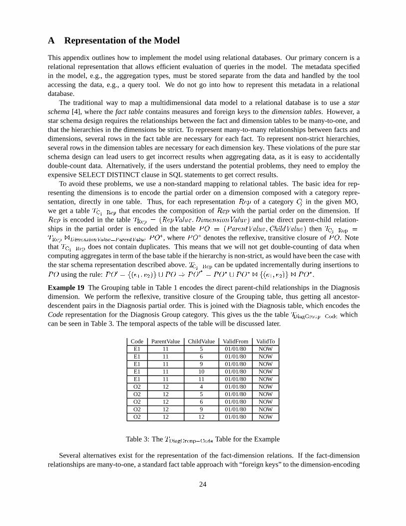
A Representation of the Model

This appendix outlines how to implement the model using relational databases. Our primary concern is arelational representation that allows efficient evaluation of queries in the model. The metadata specifiedin the model, e.g., the aggregation types, must be stored separate from the data and handled by the toolaccessing the data, e.g., a query tool. We do not go into how to represent this metadata in a relationaldatabase.

The traditional way to map a multidimensional data model to a relational database is to use astarschema[4], where thefact tablecontains measures and foreign keys to thedimension tables. However, astar schema design requires the relationships between the fact and dimension tables to be many-to-one, andthat the hierarchies in the dimensions be strict. To represent many-to-many relationships between facts anddimensions, several rows in the fact table are necessary for each fact. To represent non-strict hierarchies,several rows in the dimension tables are necessary for each dimension key. These violations of the pure starschema design can lead users to get incorrect results when aggregating data, as it is easy to accidentallydouble-count data. Alternatively, if the users understand the potential problems, they need to employ theexpensive SELECT DISTINCT clause in SQL statements to get correct results.

To avoid these problems, we use a non-standard mapping to relational tables. The basic idea for rep-resenting the dimensions is to encode the partial order on a dimension composed with a category repre-sentation, directly in one table. Thus, for each representationRep of a categoryCj in the given MO,we get a tableTCj�Rep that encodes the composition ofRep with the partial order on the dimension. IfRep is encoded in the tableTRep � �RepValue�DimensionValue� and the direct parent-child relation-ships in the partial order is encoded in the tablePO � �ParentValue�ChildValue� then TCj�Rep �TRep �DimensionValue�ParentValue PO

�, wherePO� denotes the reflexive, transitive closure ofPO. NotethatTCj�Rep does not contain duplicates. This means that we will not get double-counting of data whencomputing aggregates in term of the base table if the hierarchy is non-strict, as would have been the case withthe star schema representation described above.TCj�Rep can be updated incrementally during insertions toPO using the rule:PO� � f�e�� e��g � PO � PO�� PO� � PO�

� f�e�� e��g � PO�.

Example 19 The Grouping table in Table 1 encodes the direct parent-child relationships in the Diagnosisdimension. We perform the reflexive, transitive closure of the Grouping table, thus getting all ancestor-descendent pairs in the Diagnosis partial order. This is joined with the Diagnosis table, which encodes theCoderepresentation for the Diagnosis Group category. This gives us the the tableTDiagGroup�Code whichcan be seen in Table 3. The temporal aspects of the table will be discussed later.

Code ParentValue ChildValue ValidFrom ValidToE1 11 5 01/01/80 NOWE1 11 6 01/01/80 NOWE1 11 9 01/01/80 NOWE1 11 10 01/01/80 NOWE1 11 11 01/01/80 NOWO2 12 4 01/01/80 NOWO2 12 5 01/01/80 NOWO2 12 6 01/01/80 NOWO2 12 9 01/01/80 NOWO2 12 12 01/01/80 NOW

Table 3: TheTDiagGroup�Code Table for the Example

Several alternatives exist for the representation of the fact-dimension relations. If the fact-dimensionrelationships are many-to-one, a standard fact table approach with “foreign keys” to the dimension-encoding

24

tables will suffice. If relationships are many-to-many, there are three alternatives: a) maintain the dimensionencoding tables joined with the fact-dimension relation, with no duplicates, making the resulting table“point to” the facts, b) make a new “lowest” level in the dimension-encoding tables for eachcombinationof dimension values pointed to by one fact, and make the fact table point to the combination, and c) encodethe fact-dimension relation directly as a separate table.

Example 20 For the example above, alternative a) would maintain the join ofTDiagGroup�Code with theHas table. Alternative b) would give two combinations,f g andf�� g, which would be the bottomvalues in the extension of theTDiagGroup�Code table. The fact table would then point to these combinations,instead of the diagnoses directly. Alternative c) would just keep theTDiagGroup�Code and Has tables.

Each alternative has its own advantages. Alternative a) provides direct access to the facts, with noproblems of double-counting, but the tables can become very big, as we have several rows for each fact-dimension pair, thus rendering the solution impractical. Alternative b) is attractive if the number of combi-nations is small, as we avoid the problems of double-counting, but if the number of combinations is large,we have the same size problems as in a). Alternative c) keeps the size of the tables to the minimum, butaccidental double-counting is possible, thus SELECT DISTINCT clauses must be used in SQL statements.

When extending the representations to capture valid/transaction time, the basic dimension-encodingmechanism still works. The encoding table is extended with columns capturing the time when the tuple istrue. We take the intersection of the time periods when tables are joined, thus capturing the time periodwhen the combined tuples are valid. TheTDiagGroup�Code table extended with time is seen in Table 3.Alternative a) and c) can be extended with time columns without any problems. For alternative b) we needto enumerate all combinations of dimension valuesandthe associated time periods. This will probably leadto a number of combinations that is close to the number of facts, thus rendering the solution impractical.

When extending the representations to capture uncertainty, we just extend the tables with columnsfor the probabilities. When joining tables, the product of the probabilities is used for the resulting tuple.Alternatives a) and c) for representing the fact-dimension relations can be extended with probability columnswithout any problems. For alternative b) we need to enumerate all combinations of both the dimensionvaluesand the associated probabilities, perhaps yielding a considerably larger number of combinations.

25

multidimensional data modeling for complex...

Documents