multidimensional poverty and inequality of opportunity in ... · a child will be able to overcome...
TRANSCRIPT

June2012
Javier Escobal
Multidimensional Poverty and Inequality of Opportunity in Peru: Taking Advantage of the Longitudinal Dimension of Young Lives
WORKINGPAPERNO.79


June 2012
Javier Escobal
Multidimensional Poverty and Inequality of Opportunity in Peru: Taking Advantage of the Longitudinal Dimension of Young Lives
WORKING PAPER NO. 79
Young Lives, Oxford Department of International Development (ODID), University of Oxford,
Queen Elizabeth House, 3 Mansfield Road, Oxford OX1 3TB, UK
Funded by

Multidimensional Poverty and Inequality of Opportunity in Peru: Taking Advantage of the Longitudinal Dimension of Young Lives
Javier Escobal
First published by Young Lives in June 2012
© Young Lives 2012 ISBN: 978-1-904427-90-2
A catalogue record for this publication is available from the British Library. All rights reserved. Reproduction, copy, transmission, or translation of any part of this publication may be made only under the following conditions:
• withthepriorpermissionof thepublisher;or
• withalicencefromtheCopyrightLicensingAgencyLtd., 90TottenhamCourtRoad,LondonW1P9HE,UK,orfromanothernationallicensingagency;or
• underthetermssetoutbelow.
This publication is copyright, but may be reproduced by any method without fee for teaching or non-profit purposes, but not for resale. Formal permission is required for all such uses, but normally will be granted immediately. For copying in any other circumstances, or for re-use in other publications, or for translation or adaptation, prior written permission must be obtained from the publisher and a fee may be payable.
Available from: Young Lives Oxford Department of International Development (ODID) Universityof Oxford QueenElizabethHouse 3 Mansfield Road OxfordOX13TB,UKTel: +44 (0)1865 281751E-mail: [email protected] Web:www.younglives.org.uk
PrintedonFSC-certifiedpaperfromtraceableandsustainablesources.

MULTIDIMENSIONAL POVERTY AND INEQUALITY OF OPPORTUNITY IN PERU: TAKING ADVANTAGE OF THE LONGITUDINAL DIMENSION OF YOUNG LIVES
i
Contents List of tables ii
List of figures iii
Abstract iv
Acknowledgements iv
The Author iv
1. Introduction 1
2. The Young Lives data 4
2.1 Well-being, opportunity outcomes and circumstances in Young Lives data 4
2.2 Recent trends in unequal outcomes with respect to child well-being in Peru 9
3. Multidimensional well-being, multidimensional poverty and deprivation indices 10
3.1 Another way of looking at multidimensional poverty: the Adjusted Headcount Ratio or Multidimensional Poverty Index 13
3.1.1 Decomposing the Adjusted Headcount Ratio 14
3.2 Inequality of opportunity: measuring the Human Opportunity Index 15
3.2.1 Decomposition of changes in the Human Opportunity Index 17
4. Estimating multidimensional poverty and the Human Opportunity Index using Young Lives data 18
4.1 Aggregate multidimensional poverty 18
4.2 Measuring multidimensional poverty 22
4.2.1 Decomposing deprivations by social groups 27
4.3 Measuring the Human Opportunity Index 31
4.3.1 Looking at the Older Cohort 34
6. Concluding remarks 37
References 40
Statistical Appendix 43

MULTIDIMENSIONAL POVERTY AND INEQUALITY OF OPPORTUNITY IN PERU: TAKING ADVANTAGE OF THE LONGITUDINAL DIMENSION OF YOUNG LIVES
ii
List of tables Table 1. Selected child well-being and poverty outcomes measured in
Young Lives survey (Rounds 1 and 2) 5
Table 2. Selected child and household circumstances included in Young Lives survey 6
Table 3. Changes in selected Young Lives well-being and poverty indicators between
Rounds 1 and 2: Younger Cohort 7
Table 4. Changes in selected Young Lives well-being and poverty indicators between Rounds 1 and 2: Older Cohort 8
Table 5. Peru 2000–9: evolution of key child well-being and poverty indicators (%) 9
Table 6. Relative importance of different dimensions of child well-being as
children grow up 11
Table 7. Different definitions of multidimensional poverty: Younger Cohort (%) 19
Table 8. Different definitions of multidimensional poverty: Older Cohort (%) 19
Table 9. Multidimensional poverty in key sub-groups (second grouping):
Younger Cohort (%) (by different definitions) 22
Table 10. Decomposition of the Multidimensional Poverty Index: Younger Cohort (%)
(by household, mother and child characteristics) 23
Table 11. Decomposition of the Multidimensional Poverty Index: Younger Cohort (%)
(by region and remoteness characteristics) 24
Table 12. Relative importance of each poverty dimension: Younger Cohort (%) 25
Table 13. Decomposition of the Multidimensional Poverty Index: Older Cohort (%)
(by household, mother and child characteristics) 26
Table 14. Relative importance of each poverty dimension: Older Cohort (%) 27
Table 15. Decomposition of the Multidimensional Poverty Index: Younger Cohort (%)
(by group characteristics – first grouping, worst and best circumstances) 28
Table 16. Decomposition of the Multidimensional Poverty Index: Younger Cohort (%)
(by group characteristics – second grouping, worst and best circumstances) 29
Table 17. Decomposition of deprivation dimensions: Younger Cohort
(for key sub-groups, second grouping) 30
Table 18. Decomposition of deprivation dimensions: Older Cohort
(for key sub-groups, second grouping) 30
Table 19. Human Opportunity Index for selected outcomes: Younger Cohort,
Round 1 (%) (considering basic circumstances) I/ 31
Table 20. Human Opportunity Index for selected outcomes: Younger Cohort,
Round 1 (%) (considering extended circumstances) II/ 32
Table 21. Human Opportunity Index for selected outcomes: Younger Cohort,
Round 2 (%) (considering extended circumstances) III/ 33

MULTIDIMENSIONAL POVERTY AND INEQUALITY OF OPPORTUNITY IN PERU: TAKING ADVANTAGE OF THE LONGITUDINAL DIMENSION OF YOUNG LIVES
iii
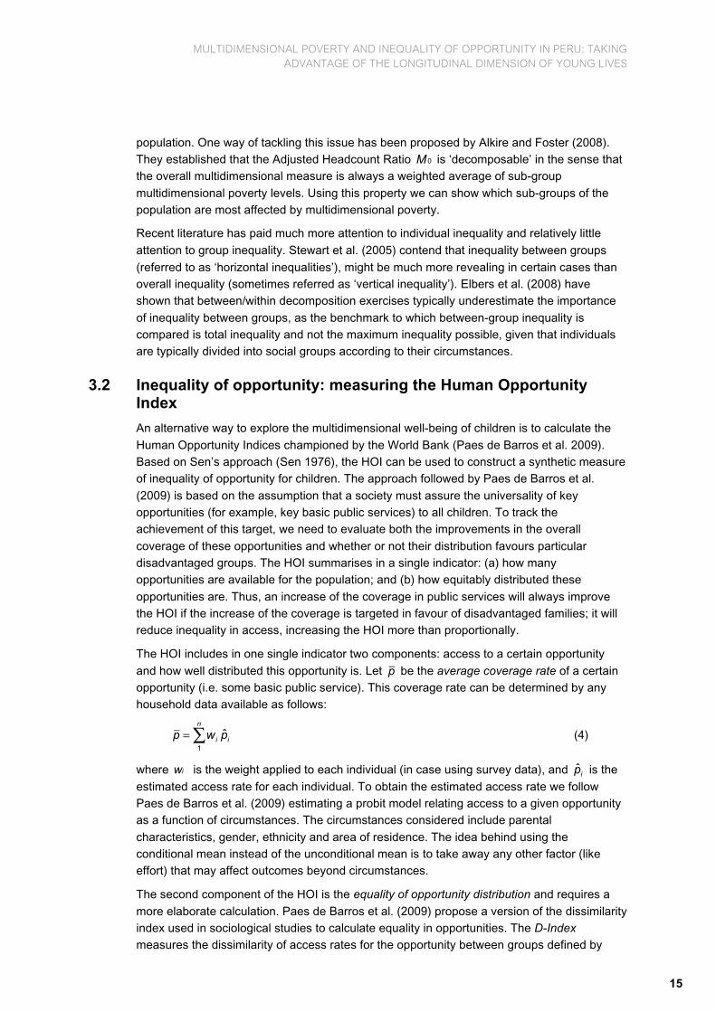
Table 22. Decomposition of Human Opportunity Index changes for selected outcomes:
Younger Cohort (considering extended circumstances) 34
Table 23. Human Opportunity Index for selected outcomes: Older Cohort,
Round 1 (%) (considering extended circumstances) II/ 34
Table 24. Decomposition of Human Opportunity Index changes for selected outcomes:
Older Cohort, Round 2 (%) (considering extended circumstances) III/ 35
Table 25. Decomposition of Human Opportunity Index for selected outcomes:
Older Cohort (%) (considering extended circumstances) 36
Table 26. Changes in Human Opportunity Index along quality dimensions:
Younger Cohort (%) 36
Statistical Appendix
Table A1. Multidimensional well-being in key sub-groups
(first grouping, showing indicators): Younger Cohort (%) 43
Table A2. Multidimensional well-being in key sub-groups (second grouping, showing
indicators): Younger Cohort (%) 44
Table A3. Multidimensional poverty in key sub-groups (first grouping, by different
definitions): Younger Cohort (%) 45
Table A4. Multidimensional poverty in key sub-groups (second grouping, by different definitions): Younger Cohort (%) 45
Table A5: Human Opportunity Index for selected outcomes, Younger Cohort,
Round 2 (%) (considering basic circumstances) I/ 46
Table A6. Human Opportunity Index for selected outcomes, Older Cohort,
Round 1 (%) (considering basic circumstances) I/ 46
Table A7. Human Opportunity Index for selected outcomes: Older Cohort,
Round 2 (%) (considering basic circumstances) I/ 47
List of figures Figure 1. Multidimensional well-being in key sub-groups (first grouping),
worst and best circumstances: Younger Cohort, Round 1 20
Figure 2. Multidimensional well-being in key sub-groups (first grouping),
worst and best circumstances: Younger Cohort, Round 2 21

MULTIDIMENSIONAL POVERTY AND INEQUALITY OF OPPORTUNITY IN PERU: TAKING ADVANTAGE OF THE LONGITUDINAL DIMENSION OF YOUNG LIVES
iv
Abstract Multidimensional poverty and inequality of opportunity are closely interconnected concepts.
Equality of opportunity levels the playing field so that circumstances such as gender,
ethnicity, geographical location or family background, which are beyond the control of a child, do not influence his or her life chances. This means that if equality of opportunity is achieved, a child will be able to overcome multidimensional poverty and deprivation. Using the
information collected in Peru during the first two rounds of the Young Lives longitudinal study, we describe how multidimensional poverty and inequality of opportunity evolve as children get older. Results show that although scalar indices of multidimensional poverty, deprivations
or inequality of opportunity may be quite useful as an advocacy tool, they may mask important heterogeneities.
Acknowledgements The paper benefited from the extensive assistance of Eva Flores. I would also like to thank
Maria Ana Lugo and Laura Camfield for valuable comments.
The Author Javier Escobal is Senior Researcher at GRADE (Grupo de Análisis para el Desarollo –
Group for the Analysis of Development) in Lima, Peru, and Principal Investigator for Young Lives in Peru.
About Young Lives
Young Lives is an international study of childhood poverty, following the lives of 12,000 children in 4 countries (Ethiopia, India, Peru and Vietnam) over 15 years. www.younglives.org.uk
Young Lives is core-funded from 2001 to 2017 by UK aid from the Department for International Development (DFID), and co-funded by the Netherlands Ministry of Foreign Affairs from 2010 to 2014.
The views expressed are those of the author(s). They are not necessarily those of, or endorsed by, Young Lives, the University of Oxford, DFID or other funders.

MULTIDIMENSIONAL POVERTY AND INEQUALITY OF OPPORTUNITY IN PERU: TAKING ADVANTAGE OF THE LONGITUDINAL DIMENSION OF YOUNG LIVES
1
1. Introduction Equality of opportunity has increasingly captured the attention of policymakers. Recently,
international organisations like the World Bank and UNDP have included specific indicators
to trace inequality in access to key public goods and services (see Paes de Barros et al. 2009 and UNDP 2007). Unlike equality of outcome, in which one seeks to reduce or eliminate differences in material condition between individuals or households in a society,
equality of opportunity aims to level the playing field so that circumstances such as gender, ethnicity, birthplace, maternal education or any other aspect of family background, which are beyond the control of an individual, do not influence a person’s life chances.
The literature recognises that inequality may include many dimensions. Some authors tend to focus on inequality in terms of outcomes like income, consumption, access to education and
access to work, and measure it accordingly. Others, such as Sen (1985), have advocated the need to look at activities and states that make up people’s well-being, taking into account a wider range of outcomes, including elementary ones, such as being in good health and
properly nourished and sheltered, and social outcomes such as having self-respect or taking part in the life of the community. Yet others, such as Roemer (1998), have emphasised the fact that inequality of opportunity should be measured in such a way that it is independent of
an individual’s circumstances, and is a function only of their effort.
In an ideal world, children’s chances of success in life would depend on their effort, talent
and choices and not on their circumstances at birth or other circumstances beyond their control. While outcomes can usually be measured with a considerable degree of precision,
opportunities cannot. However, when we look at children – especially at an early age – it is more likely that it is circumstances and not effort that are determining their well-being. Something different may happen as the children grow up to become young people and
adults. In those cases we might expect that effort would play an increasing role as a determinant of their well-being. Therefore, the best group to use to evaluate how these initial circumstances affect opportunities in life is young children, given that at very early ages the
effort component is very small.1
Several indicators have been constructed to try to measure inequality of opportunity.
Following the work of Roemer (1998), which distinguishes between ‘circumstances’ and ‘effort’, authors like Lefranc et al. (2006) have developed statistical tests to compare the distribution of opportunities between individuals with similar circumstances. Ruiz-Castillo
(2003) and Bourguignon et al. (2003) followed a complementary approach and constructed a scalar index of inequality of opportunity, based on dividing the population according to such categories of circumstances as parents’ education, occupation and race. This index has been
adapted and used in several World Bank publications including Paes de Barros et al. (2009), who used it to evaluate inequality of opportunity among children in Latin America.
A closely related concept of inequality of opportunity is that of experiencing deprivations.
Gordon et al. (2003) introduced the concept of deprivations, highlighting the multidimensional
nature of poverty in general and child poverty in particular. These authors constructed a
1 One may wonder, however, if equality of opportunity for children can be achieved without greater equality of outcome for
parents.

MULTIDIMENSIONAL POVERTY AND INEQUALITY OF OPPORTUNITY IN PERU: TAKING ADVANTAGE OF THE LONGITUDINAL DIMENSION OF YOUNG LIVES
2
poverty headcount based on counting children with two or more severe deprivations. The gauge included seven indicators: appropriate shelter; sanitation facilities; safe drinking water; adequate nutrition as reflected by not being stunted, wasted or undernourished; school
attendance; adequate immunisation coverage; and access to information sources like radio, television, telephone, newspaper or computer. In 2007, UNICEF fully acknowledged the multidimensional nature of child poverty. The January 2007 UN General Assembly stated, in
its annual resolution on the rights of the child, that ‘Children living in poverty are deprived of nutrition, water and sanitation facilities, access to basic healthcare services, shelter, education, participation and protection, and that while a severe lack of goods and services
hurts every human being, it is most threatening and harmful to children, leaving them unable to enjoy their rights, to reach their full potential and to participate as full members of the society’ (UNICEF 2007: 11).
In Peru, inequality in general, and inequality of opportunity in particular, has increasingly
captured the attention of researchers and policymakers.2 Although there is some evidence that income inequality has been decreasing in recent years (Jaramillo and Saavedra 2009; Lopez-Calva and Lustig 2009) this reduction is small when compared to the high level of
income inequality prevailing in Peru, and it masks important inequality trends along other relevant dimensions such as location (urban/rural/remote), ethnicity and life stage. For example, although income inequality, as measured by the Gini coefficient, may show a very
small decline, the gap in income or in other well-being dimensions between urban/rural areas is increasing. Figueroa and Barrón (2005) and Barrón (2008) suggest that inequality along the ethnic divide may be increasing. Escobal and Ponce (2010) show that while income
inequality, measured by a Gini coefficient, diminished between 1993 and 2007, during the same period geographic polarisation of well-being increased. Similarly, Muñoz et al. (2007) show that inequalities between groups continue to be very high. In relation to child well-
being, data available from INEI, the Peruvian national statistics agency (2010), show that although the gap between the top 20 per cent and bottom 20 per cent of the income distribution has been reduced in the last decade in important poverty (or lack of well-being)
indicators such as chronic malnutrition or low weight at birth, it continues to be large and is increasing in other relevant dimensions such as prevalence of acute respiratory infections, or access to key services like full immunisation.
We believe that inequality of opportunity should not be analysed taking each opportunity or
outcome in isolation from other relevant outcomes. Instead we need to recognise that children who share a certain set of circumstances may be simultaneously deprived in several well-being dimensions, and inequality in accessing one particular opportunity may be
correlated with inequality in accessing several other opportunities. In addition, an indicator of multiple deprivations should allow us to focus on the deprivations of groups in specific circumstances, in order to target them with relevant policies.
In this paper we explore different dimensions and complexities of deprivations and inequality (or equality) of opportunity for children in Peru, using the Young Lives sample. Young Lives is
an international study carried out in four countries (Ethiopia, Vietnam, India and Peru), whose objective is to improve our understanding of the causes and consequences of childhood poverty and to examine how circumstances and government policies affect children’s well-
being over time. Young Lives has been tracking 2,000 Peruvian children from a Younger
2 Equality of opportunity was the central campaign slogan of one of the candidates running in the 2011 presidential election.

MULTIDIMENSIONAL POVERTY AND INEQUALITY OF OPPORTUNITY IN PERU: TAKING ADVANTAGE OF THE LONGITUDINAL DIMENSION OF YOUNG LIVES
3
Cohort, who were aged between 6 months and 18 months in 2002, when the study began. The study also tracks an Older Cohort of about 700 children who were aged between 7.5 and 8.5 years old in 2002. The second round of data gathering was carried out between late 2006
and early 2007, and the third round between August 2009 and January 2010.
The benefits of looking at inequality of opportunity using the lens provided by the Young
Lives data are two-fold. First, in comparison with traditional surveys like the Living Standard Measurement Surveys or the Demographic and Health Surveys, Young Lives covers a wide
range of well-being indicators for the sampled children, including physical health, nutrition, education and material wealth of their parents, as well as maternal psychosocial well-being (self-esteem and sense of efficacy, sense of discrimination, etc.). This range of well-being
indicators is seldom covered in national representative samples, which typically need to narrow their focus towards people’s ability to access to basic services. By looking at a broad range of indicators, we can identify whether inequality of opportunity is affecting the various
dimensions of child well-being differently. A second benefit of using Young Lives data is that of taking advantage of the longitudinal nature of the sampling framework. Although the original sampling framework allows us to be statistically representative of the Peruvian
children of the two cohorts at the time the sampling was done, following children over time allows us to incorporate different outcome indicators as they grow up. In addition, we are able to track individual trajectories and evaluate whether or not replacing these individual
trajectories with looking at averages over time may mask increasing inequality among children. The longitudinal nature of the data allows us to understand better why inequality of opportunity may be increasing or decreasing, as we are able to control for individual and
community fixed non-observables that are typically embedded in repeated cross-sectional data.
In this paper we use a variety of indicators to track multidimensional poverty and inequality of
opportunity. First, we use aggregate indicators of multidimensional poverty and deprivations.
Next we use the methodology developed by Paes de Barros et al. (2009) to measure a person’s chances of success in life in different dimensions like schooling and health. This measure is called the Human Opportunity Index (HOI). The HOI controls for previous
circumstances or a child’s background to determine their chances of success in life.
Although any scalar index of poverty, deprivations or inequality of opportunity may be useful
as an advocacy tool, this paper shows that it may mask important heterogeneities that make it insufficient to show the full scope and depth of inequality of opportunity. Looking at a broad range of indicators, evaluating how opportunities and deprivations are unevenly distributed
across a sample of children, and showing that circumstances are correlated are crucial to address inequality properly. In this context we need to look not just at differences in opportunities or deprivations between those who are affected by a certain circumstance and
those who are not, but also at these indicators within groups of children affected simultaneously by a range of circumstances. This range of circumstances may not be isolated and specific, but may be related to broad patterns of discrimination.
Having children as a target population for these indicators brings children’s issues and needs
into the arena of policy. Exploring whether or not inequality of opportunity widens at early stages of life will allow us to engage in a policy debate associated with the costs and benefits
of early childhood development programmes.
The paper is divided into five sections. Section 2, after this introduction, presents briefly the
Young Lives data used, stressing the importance of capturing a wide range of variables that

MULTIDIMENSIONAL POVERTY AND INEQUALITY OF OPPORTUNITY IN PERU: TAKING ADVANTAGE OF THE LONGITUDINAL DIMENSION OF YOUNG LIVES
4
can cover the range of functionings that are relevant for children at different stages of their lives. Section 3 discusses alternative multidimensional poverty and deprivation indices, including those suggested by Chakravarty et al. (1998), Bourguignon and Chakravarty (2003)
and Alkire and Foster (2008). Next it presents the HOI championed by the World Bank. In Section 4, we estimate multidimensional poverty indices and the HOI to analyse Peruvian Young Lives data for both the Younger and Older Cohorts for the first two survey rounds
(2002 and 2006–7). Finally in Section 5, we discuss the importance of looking beyond single scalar indices of inequality of opportunity or multidimensional poverty by considering which poverty dimensions matter for whom.
2. The Young Lives data Young Lives is an innovative long-term international research study that investigates the
changing nature of childhood poverty. By making publicly available the information gathered,
the project seeks to improve understanding of the causes and consequences of childhood poverty, to examine how government policies affect children’s well-being, and to inform the development and implementation of future policies and practices aimed at reducing
childhood poverty. Since 2002, the study has been tracking 2,860 children in Peru through quantitative and qualitative data collection and through research, and will continue to do so over a 15-year period. The study collects information at the child, household and community
level, covering a range of issues that determine and affect the welfare of children.
The depth and extent of the Young Lives database is unique. No longitudinal research of this
size, scope and complexity has ever been undertaken in the developing world. The project not only collects data on underlying processes and outcomes associated with child poverty, but also gathers qualitative information that allows a very rich and in-depth analysis of
children’s lives and how they are affected by poverty and government policies.
In Peru, the Young Lives team used multistage, cluster-stratified, random sampling to select
the two cohorts of children. This methodology, unlike the one applied in the other Young Lives countries, randomises sentinel sites as well as households within sentinel site
locations. To ensure the sustainability of the study, and for resurveying purposes, a number of well-defined sites were chosen. These were selected with a pro-poor bias, ensuring that randomly selected clusters of equal population excluded districts located in the top 5 per cent
of the poverty map developed in 2000 by FONCODES (the Fondo Nacional de Cooperacion para el Desarrollo – National Fund of Cooperation for Development). Details about the sampling frame and sampling weights can be found in Escobal and Flores (2008).
2.1 Well-being, opportunity outcomes and circumstances in Young Lives data
Table 1 shows the indicators in the Young Lives survey that can be used to assess inequality
of opportunity for children in Peru. The survey includes a range of child, household and community characteristics that can be used to control for circumstances when calculating the HOI, shown in Table 2.
As we have mentioned, obtaining an empirical approximation of inequality of opportunity for
children involves the difficult task of classifying available indicators into ‘outcomes’, ‘circumstances’ and ‘efforts’. Although when children are very young, most of the outcomes

MULTIDIMENSIONAL POVERTY AND INEQUALITY OF OPPORTUNITY IN PERU: TAKING ADVANTAGE OF THE LONGITUDINAL DIMENSION OF YOUNG LIVES
5
are the result of circumstances, as effort on the part of the child is not considered relevant, we may still need to acknowledge that circumstances can also encompass situations where some parental outcomes are directly related to parental efforts. Here we exclude some
parental outcomes (like income) as they should be considered circumstances from the child’s point of view. On the other hand, access to key services (like electricity, water and sanitation, and vaccination) could be considered circumstances, but at the same time they are
outcomes in terms of child well-being, even if children have absolutely no control over them. We acknowledge however that the distinction between outcomes and circumstances is never an easy one.
Table 1. Selected child well-being and poverty outcomes measured in Young Lives survey (Rounds 1 and 2)
Younger Cohort Older Cohort
Round 1 Round 2 Round 1 Round 2
Mother had access to pre-natal care X
Child was ever breastfed X X X X
Child has vaccination card X
Access to electricity X X X X
Access to water piped into dwelling X X X X
Access to safe drinking water (public network) X X
Sanitation facilities (flush toilet or septic tank) X X X X
Chronic malnutrition (WHO 2006) stunting X X X X
Global malnutrition (WHO 2006) underweight X X X X
Child consumed protein in last 24 hours X X
Child experienced positive child-rearing practices X X
Child attended a childcare centre X X
Pre-school enrolment (child has attended pre-school regularly since age 3)
X X
School enrolment (child is enrolled in school) X X X
Verbal and maths skills X X X
Child is not over-age (above the age expected for their grade) X X
Cognitive ability (standardised PPVT)a X X
Child does paid work X X
Subjective well-being (child perception) X X
Respect from adults in his/her community X X
a Peabody Picture Vocabulary Test.

MULTIDIMENSIONAL POVERTY AND INEQUALITY OF OPPORTUNITY IN PERU: TAKING ADVANTAGE OF THE LONGITUDINAL DIMENSION OF YOUNG LIVES
6
Table 2. Selected child and household circumstances included in Young Lives survey
Younger Cohort Older Cohort
Round 1 Round 2 Round 1 Round 2
Gender X X X X
Maternal education X X X X
Household income X X X X
Maternal marital status X X X X
Number of children in the household X X X X
Lives in a rural area X X X X
Mother's age (in years) X X X X
Mother’s first language (Spanish or indigenous) X X X X
Maternal migration status X X X X
Maternal body mass index (BMI) X X X X
Wealth index (standard YL index)a X X X X
Region (coast, mountains, jungle) X X X X
Altitude (metres above sea level) X X X X
Travel time to nearest educational facility X X X X
Travel time to nearest health facility X X X X
a The wealth index is a simple average of the following three components: a) housing quality, which is the simple average of rooms per person, floor, roof and wall; b) consumer durables, being the scaled sum of consumer durable dummies; and c) services, being the simple average of drinking water, electricity, toilet and fuel, all of which are 0–1 variables.
As has been documented (see Escobal et al. 2008) large numbers of the Young Lives
children (80 per cent) live below the national poverty line. This high proportion is due in part to the pro-poor sampling strategy followed by the Young Lives study. Still, between Rounds 1
and 2 of data collection (2002 and 2006/7), we observed some improvement in household living standards for both the Younger and the Older Cohort across several indicators. Most of these improvements were found in urban areas, thus closely resembling Peru’s national
trends over the same period, and pointing to the inequalities that persist despite recent economic growth.
Tables 3 and 4 show the changes in child well-being and poverty indicators when we
compare Rounds 1 and 2; the pattern is mixed. At the household level all indicators show an improvement. Further, the subjective assessment of mothers and caregivers coincides with
this improvement in material well-being, as a reduced percentage feel poor or destitute and a higher percentage said in Round 2 that they could ‘manage to get by’.3 Similar results can be found for the Older Cohort (Table 4). Similarly, access to electricity and to sanitation facilities
improved between the two rounds, improving the availability of key services to Young Lives children.
3 The relevant questions reads: ‘During this period, how would you describe the household you were living in? 01=Very rich; 02=Rich; 03=Comfortable – manage to get by; 04=Struggle – never have quite enough; 05=Poor; 06=Destitute’.

MULTIDIMENSIONAL POVERTY AND INEQUALITY OF OPPORTUNITY IN PERU: TAKING ADVANTAGE OF THE LONGITUDINAL DIMENSION OF YOUNG LIVES
7
Table 3. Changes in selected Young Lives well-being and poverty indicators between Rounds 1 and 2: Younger Cohort
Round 1 Round 2 Significance levels
Household well-being indicators
Wealth index 0.39 0.41 **
Per capita food consumption (soles) 62.81 102.6 ***
Real per capita food consumption (soles) 69.58 106.5 ***
Asset value at median prices: 12 assets (soles) 759.2 883.7 *
Asset value at median prices: 22 assets (soles) 850 1,073 ***
Well-being perception in the household (%)
Can manage to get by 27.2 37.0 ***
Poor/destitute 32.2 21.9 ***
Access to services (%)
Access to electricity 59.4 69.9 ***
Access to water piped into dwelling 54.0 58.9 **
Sanitation facilities (flush toilet or septic tank) 38.0 42.0 **
Child-related well-being and poverty indicators (%)
Mother had pre-natal care 92.5 –
Low weight at birth 5.7 –
Has a vaccination card 89.1 97.0 ***
Chronic malnutrition (WHO 2006) stunting 30.9 37.4 ***
Global malnutrition (WHO 2006) underweight 7.2 5.9 *
Consumed protein in the last 24hrs – 91.3
Experienced positive child-rearing practices 68.9 31.2 ***
Attended a childcare centre 4.0 19.5 ***
Pre-school enrolment (has attended pre-school regularly since age 3) – 81.5
Low cognitive ability (standardised PPVT) – 70.8
Note: Sample averages and significance levels include sample design. Sample differences are: * significant at 10%; **significant at 5%; ***significant at 1%. Source: Young Lives.
Despite this improvement in dwelling and household indicators, child nutritional indicators
show some deterioration between rounds. Among them key nutritional outcomes like stunting
(low height-for-age) and underweight (low weight-for age) stand out. As has been noted by Escobal et al. (2009), we can expect deterioration in these indicators as children get older because children tend to depart from the ‘normal growth curve’.4 However when we explore
changes in these indicators for different sub-groups we can find that some groups (for example, urban children born to educated mothers) show some evidence of catching up, something that is not apparent in rural children.
4 The WHO reference population was purposely designed to reflect the growth curve of healthy children living in conditions
adequate to fulfill their genetic growth potential.

MULTIDIMENSIONAL POVERTY AND INEQUALITY OF OPPORTUNITY IN PERU: TAKING ADVANTAGE OF THE LONGITUDINAL DIMENSION OF YOUNG LIVES
8
Table 4. Changes in selected Young Lives well-being and poverty indicators between Rounds 1 and 2: Older Cohort
Round 1 Round 2 Significance levels
Household well-being indicators
Wealth index 0.36 0.37 *
Per capita food consumption (soles) 16.2 22.8 **
Real per capita food consumption (soles) 18.3 24.2
Asset value at median prices: 12 assets (soles) 471.7 589.6 **
Asset value at median prices: 22 assets (soles ) 604.8 764.8 **
Well-being perception in the household (%)
Can manage to get by 25.0 27.4 **
Poor/destitute 36.1 28.5 ***
Access to services (%)
Access to electricity 54.9 64.8 ***
Sanitation facilities (flush toilet or septic tank) 28.1 34.3 **
Child-related well-being and poverty indicators (%)
Chronic malnutrition (WHO 2006) stunting 34.5 41.8 **
Global malnutrition (WHO 2006) underweight 6.1 –
Enrolled in school 99.2 99.0
Verbal skills 42.6 79.6 ***
Maths skills 47.0 93.4 ***
Does paid work 24.1 31.0
Over-age for school grade 30.7 24.0 *
Respect from adults in his/her community 76.9 95.3 ***
Subjective well-being child perception (on a scale from 1 to 9) – 4.76
Note: Sample averages and significance levels include sample design. Sample differences are: * significant at 10%; **significant at 5%; ***significant at 1%. Source: Young Lives.
Other child-related well-being and poverty indicators show a mixed pattern. Among the
Younger Cohort there is an increase in vaccination coverage and in attendance at childcare centres. However the percentage of mothers who implement ‘positive’ child-rearing practices
is reduced substantially. Among these practices, which have been shown to affect child well-being positively and are included in the survey are: (1) adequate child feeding practices (including breastfeeding and complementary feeding when appropriate); and (2)
psychosocial care, associated with ‘the provision of affection and warmth, responsiveness to the child, and the encouragement of autonomy and exploration’ (Engle et al. 1999: 1,327). In the case of the Older Cohort, we find significant improvement in age for school grade and in
mathematical and verbal skills (although these ‘improvements’ really reflect the fact that some children have caught up on some basic skills that should have been learned at a younger age). In addition, this cohort increasingly reports obtaining respect from adults in
their community. The data also show changes associated with increases in paid child work as well as an increase in stunting.

MULTIDIMENSIONAL POVERTY AND INEQUALITY OF OPPORTUNITY IN PERU: TAKING ADVANTAGE OF THE LONGITUDINAL DIMENSION OF YOUNG LIVES
9
2.2 Recent trends in unequal outcomes with respect to child well-being in Peru
Although Young Lives follows the same children as they grow older and shows changes in inequality, we can also explore some trends in inequality in child well-being by looking at
repeated cross-sections of nationally representative data. Using INEI (2010) data, Table 5 shows that in several key indicators related to health and nutrition, as well as access to basic services, the gap between children living in households located in the richest 20 per cent and
the poorest 20 per cent of Peruvian population has narrowed.
This narrowing gap is partly due to the fact that the top 20 per cent have full or almost-full
coverage of services, and the poorest are starting to receive some access. It might also reflect improved targeting, as the National Strategy for Poverty Reduction, known as
CRECER (‘to grow’) aimed at fighting poverty and childhood malnutrition was put into place in 2007, and pushed for better coordination of programmes developed by ministries in different social sectors (e.g. Health, Education, and Women and Social Development).
Table 5. Peru 2000–9: evolution of key child well-being and poverty indicators (%)
2000 2005 2007 2008 2009
Stunting (chronic malnutrition) (NCHS/aCDC/
bWHO standard) 25.4 22.9 22.6 21.5 18.3
Urban 13.4 9.9 11.8 11.8 9.9
Rural 40.2 40.1 36.9 36.0 32.8
Bottom 20% – 46.8 45.1 45.0 37.1
Top 20% – 4.3 4.2 5.4 2.3
Stunting (chronic malnutrition) (WHO standard) – 28.0 28.5 27.5 23.8
Urban – 13.5 15.6 16.2 14.2
Rural – 47.1 45.7 44.3 40.3
Bottom 20% – 55.2 53.5 54.6 45.3
Top 20% – 4.7 5.9 8.1 4.2
Low weight at birth (<2.5 kg) (WHO standard) – 8.7 8.4 7.2 7.1
Urban - 7.8 7.7 6.4 6.6
Rural - 10.6 9.5 8.9 8.4
Bottom 20% - 12.1 11.7 10.3 8.9
Top 20% - 5.4 7.2 4.8 4.9
Access to safe water 84.4 92.1 92.9 93.8 91.1
Urban 93.9 97.3 96.8 97.9 96.3
Rural 68.1 81.7 85.3 85.9 80.4
Bottom 20% N.A. 66.8 63.8 69.7 73.6
Top 20% N.A. 99.7 100.0 100.0 99.9
Access to sanitation 75.9 80.5 81.8 85.0 83.3
Urban 91.7 95.7 92.4 93.3 92.3
Rural 48.6 50.8 61.0 68.8 64.7
Bottom 20% N.A. 37.4 35.8 44.1 54.9
Top 20% N.A. 100.0 99.9 99.9 100.0
a National Center for Health Statistics. b Centers for Disease Control and Prevention. Source: INEI (2010).

MULTIDIMENSIONAL POVERTY AND INEQUALITY OF OPPORTUNITY IN PERU: TAKING ADVANTAGE OF THE LONGITUDINAL DIMENSION OF YOUNG LIVES
10
In addition to reductions in the gaps related to stunting, low weight at birth and access to
services, INEI (2010) reports reductions in the coverage gap between children in the top 20 per cent and in the bottom 20 per cent of the income distribution for acute diarrhoea, pre-
natal check-ups, delivery in a health institution and growth monitoring. Despite these gap reductions, inequality is increasing in other dimensions like possession of identity cards (which allow the children to get healthcare under the public health programme), access to full
immunisation and prevalence of acute respiratory infections, where the gap between rich and poor children has increased. These data indicate that inequality of opportunity for children is a complex phenomenon, since the gap between rich and the poor children may decrease in
some dimensions while it may be widening in others.
In addition, these results are only useful to show an ‘average’ picture, as official statistics are
unfortunately not able to focus on children as the relevant unit of analysis, nor to account for their multidimensional experience. For example, if we have two well-being dimensions, and
50 per cent of these children cover one dimension while the other 50 per cent cover the other dimension, using official statistics we cannot distinguish this case from a case where 50 per cent of children are covering both dimensions while the other 50 per cent of children are not
able to satisfy either dimension. In both cases, the average coverage in each dimension will be 50 per cent. This example highlights the fact that we need to study child well-being looking at how children individually experience the multidimensional nature of their well-
being, as aggregate data blur the picture and may hide important inequalities. This is precisely why Young Lives data are well positioned to shed light on the multidimensional nature of inequality of opportunity.
3. Multidimensional well-being, multidimensional poverty and deprivation indices As we have seen, child well-being evolves differently along different dimensions. We can
recognise that children’s well-being depends on (a) physical health and nutritional status; (b) the development of pro-social skills and competences (life skills beyond educational
achievement measures); and (c) the consolidation of self-esteem and the ability and opportunity to make their own decisions. Household material well-being and access to services can be considered as inputs for generating these three outcomes.
Further, we need to acknowledge the fact that the relative importance of different dimensions of child well-being changes as children grow older. As we depict in Table 6, we can expect
that health and nutrition are relatively more important during the first years of life. Later in life, between 6 and 11 years old, education and capacity-building competences become increasingly important. Later still (between 12 and 17 years old) social and environmental
opportunities and risks are relatively more important (Lynch 2003; Strauss and Thomas 2007).

MULTIDIMENSIONAL POVERTY AND INEQUALITY OF OPPORTUNITY IN PERU: TAKING ADVANTAGE OF THE LONGITUDINAL DIMENSION OF YOUNG LIVES
11
Table 6. Relative importance of different dimensions of child well-being as children grow up
Age Groups Health & Nutrition Education & capacity building
Social & environmental risks & opportunities
0–5 years
6–11 years
12–17 years
Key: = important; = less important; = not very important.
Even within each of these dimensions, the indicators relevant for each age group can vary.
For example, at the beginning of children’s lives vaccination is important, while later in life
sexual and reproductive health becomes important. Similarly pre-school enrolment and being over-age for one’s school grade are variables to look at different stages in life when considering the educational dimension. Good child-rearing practices also change with the
age of the child.5 In some cases certain dimensions may need to be age-specific in order to get a better assessment of well-being or inequality in opportunities. For example, certain verbal or mathematical abilities may be appropriate for certain age groups.
Given that there are many dimensions relevant to measuring the well-being of a child, and
that each of these dimensions may be captured with a different range of indicators depending on the age of the children, one wonders why we really need a single multidimensional indicator of child poverty. The use of a unique multidimensional index has been championed
by UNICEF since early 1990s, on the basis that the Human Development Index can illustrate ‘how powerful one composite index can be in bringing attention to critical policy issues’ (UNICEF 2007: 19). UNICEF has also championed the need to provide a unique and ‘simple’
indicator of child well-being, claiming that it is extremely helpful for policy planning, targeting and monitoring. As we contend in this paper, such an aim for simplicity may be unhelpful.
Although they have been typically portrayed as improved alternatives to monetary measures
of poverty, several of the poverty indices that appear in the literature have been constructed without careful attention to the complexities of well-being aggregation. Are the dimensions
complements or substitutes? Are minimum thresholds of certain indicators absolutely essential to define a minimum standard that can be socially acceptable? These types of questions are very much related to specific ways in which dimensions could be aggregated in
a meaningful way.
If the index has been constructed based solely on statistical procedures that capture the
maximum variability of the sample, as is typical when one constructs implicit weights through factor or principal component analysis (Nardo et al. 2005), it may be extremely difficult to
interpret the resulting index, as it is hardly the case that the more variance some indicator has, the more important it is in terms of the well-being of the children.
5 To explore child-rearing practices in Round 1, the following question was included: ‘When the child cries, what do you do? (breastfeed him/her; shout at or threaten him/her verbally; use physical violence; use other negative behaviours; do nothing)?’
In Round 2, the question was changed to reflect the age of the child: ‘When the child cries, what do you do? (talk to him/her,
scold him/her; ground him/her; shout or threaten him/her verbally; use physical violence; do nothing)?’

MULTIDIMENSIONAL POVERTY AND INEQUALITY OF OPPORTUNITY IN PERU: TAKING ADVANTAGE OF THE LONGITUDINAL DIMENSION OF YOUNG LIVES
12
To clarify this, let’s put forward a hypothetical example. Suppose that the children are
distributed in our sample as follows: Children have toys
NO YES
Children have enough food Children have enough food
NO YES NO YES
Children have a pencil NO 0 60 5 35
YES 5 35 10 50
Here half of a sample of children lacks pencils, half of the sample lacks toys and ‘just’ 10 per
cent of the sample lacks minimum food requirements. If one performs the classic principal
component analysis to extract a linear combination of the three variables that contain most of the variance and use that indicator to rank children‘s well-being, children that have pencils and toys but not food will be ranked higher than those that have food but have no pencils or
toys. This is so because there is a larger variance that can be extracted from the pencil and toys variables.6 This example shows that when there are trade-offs between different well-being dimensions, it is the explicit consideration of these trade-offs and not an empirical
regularity that should drive any conclusion regarding well-being rankings.
There are many ways in which these trade-offs can be taken into consideration. Bourguignon
and Chakravarty (2003), for example, make a distinction between ‘intersection’ and ‘union’ definitions of poverty. These authors argue that if we measure well-being in more than one dimension, then a person can be considered poor if he or she is poor in any dimension. They
define this as a ‘union’ definition of multidimensional poverty. Alternatively, an intersection definition would consider a person to be poor only if he or she was poor in all dimensions at the same time. Either of these two indicators of multidimensional well-being may be
considered valid as far as we agree with the benchmark used.7
Considering D different dimensions of well-being, the union headcount index for
multidimensional poverty (M) can be calculated as follows:
M(Xi ,Z) = 1− I(z j < xi , j )j=1
j=D
∏ (1)
while the intersection headcount index can be calculated as follows:
M(Xi ,Z) = I(z j > xi , j )
j=1
j=D
∏ (2)
If one is interested in considering intermediate cases, we can calculate a multidimensional poverty indicator as a weighted mean of poverty levels by attribute. If this is the case,
Chakravarty et al. (1998) derive the following index:
M(Xi ,Z) = aj
z j − xi , j
z j
⎛
⎝⎜
⎞
⎠⎟
j=1
j=D
∑+
α
(3)
6 The 50/50 distribution of the sample between those that have and have not got pencils and toys will generate the maximum possible variance for dichotomous variables.
7 Note that if enough relevant dimensions are taken, virtually everyone could be judged poor by the union definition.

MULTIDIMENSIONAL POVERTY AND INEQUALITY OF OPPORTUNITY IN PERU: TAKING ADVANTAGE OF THE LONGITUDINAL DIMENSION OF YOUNG LIVES
13
This measure is simply a multidimensional extension of Foster et al.’s (1984) FGT (Foster,
Greer, Thorbecke) measure with vector of well-being dimensions Yi= (xi,1,..., xi,D) and vector of poverty lines (zj), determining i’s contribution to total multidimensional poverty M(Yi, Z). aj
stands for the relative importance of each of the D well-being dimensions being considered and α is a measure of the aversion with respect to any dimension. Here the choice of aj is critical, as different dimensions may be considered more or less important for the well-being
of the child. In a way similar to any FGT measure, this indicator captures how far an individual is from achieving a minimum requirement in a particular dimension.
These indices are individual poverty measures and they will need to aggregate across all
individuals. Such aggregation can be a simple average. However the formula will need to
satisfy the multidimensional transfer principle.
3.1 Another way of looking at multidimensional poverty: the Adjusted Headcount Ratio or Multidimensional Poverty Index
Many aggregate measurements have been developed focusing mainly on aggregating
different well-being dimensions into one single indicator. The work of Alkire and Foster (2008) focuses on a prior step needed to construct such an indicator. This step is the
identification of who is really poor. Conceptually this approach is similar to that proposed by Bourguignon and Chakravarty (2003) when presenting ‘intersection’ and ‘union’ poverty indicators. Using an intuitive approach, Alkire and Foster (2008) generalise this type of
indicator by establishing two consecutive cut-offs. The first is the traditional dimension-specific poverty line, which is established for each of the dimensions being considered. The second establishes how widely deprived a person must be in order to be considered poor.
This second cut-off point may generate the intersection poverty indicator if we establish a demanding cut-off point (a child needs to be poor or deprived in all dimensions in order to be considered multidimensionally poor). Alternatively it may generate the union poverty indicator
if the cut-off point is low enough as to consider a child as multidimensionally poor if she is poor in at least one dimension.
Suppose we have n number of persons in the population and let d ≥ 2 be the number of
dimensions under consideration. Let Y = [Yij ] denote the n x D matrix of well-being
outcomes, where the typical entry Yij is the achievement of the individual i = 1, 2,..., n in dimensions j =1, 2,…, D. Let zj denote the cut-off below which a person is considered to be deprived in dimension j .
To measure multidimensional poverty or multidimensional well-being we need to first identify who is poor and then construct a consistent aggregating function, like the one we presented
in equations (1), (2) and (3). Here we transform the data matrix from outcomes to deprivations g(0) (instead of achievements, or being not poor). Here
ij
0g = 1 when Yij < zj while, and
ij
0g =0 otherwise.
To help understand this notation we present the same example as the one presented by
Alkire and Foster (2008). Here we have four persons and four well-being dimensions. Further, each dimension has its corresponding cut-off point zj, below which the child may be considered poor or deprived in that dimension:

MULTIDIMENSIONAL POVERTY AND INEQUALITY OF OPPORTUNITY IN PERU: TAKING ADVANTAGE OF THE LONGITUDINAL DIMENSION OF YOUNG LIVES
14
Dimensions Deprivations ci
y =
13.1 14 4 115.2 7 5 012.5 10 1 020 11 3 1
children
g0 =
0 0 0 00 1 0 11 1 1 11 1 0 0
0241
z ( 13 12 3 1 ) Cut-offs
For matrix 0g we can construct an extra vector that sums the number of deprivations per
person in the population (cj). For k = 1, …,D; let k
p be the identification method defined by
kp ( Yi , zj )=1 whenever ci >k and kM ( Yi , zj )=0 whenever ci < k .
In a way similar as the one presented in equation (3), based on rationale behind FGT
indicators, we can use a cut-off level k that lies between 1 and D to say that a person is multidimensionally deprived if the number of deprivations is larger than this cut-off level. In other words, a person i is poor when the number of dimensions in which i is deprived is at
least k . This method is known as the dual cut-off method of identification.
To start measuring poverty, a common way is to calculate the percentage of poor people.
The headcount ratio H ( yi , z ) is defined by H = q / n , where q = q ( yi , z ) is the number of persons in the set Zk , and therefore the number of poor people identified using the dual cut-off approach. Following the example, given a cut-off of k ≥2, we would have 2 persons
who are defined as ‘poor’, thus our poverty rate would be 50 per cent8 of the population qualifying as poor.
What happens once we raise k to 3, meaning k ≥3? The poverty rate stays the same,
hence the dimensional monotonicity property has not been satisfied. Attending to this
concern, Alkire and Foster have defined an Adjusted Headcount Ratio M 0 as a Multidimensional Poverty Index (MPI). It is a measure that is sensitive to the frequency and the extent of multidimensional poverty that satisfies the monotonicity property. In other
words, the Adjusted Headcount Ratio is the total number of deprivations experienced by poor people, divided by the maximum number of deprivations that could possibly be experienced by all people.
Going back to the example mentioned above: keeping up the cut-off at k ≥2, we would have
6 (2+4) experienced deprivations divided by the 16 maximum possible deprivations of the population (4 deprivations, for 4 persons), giving us 37.5 per cent of the population qualifying as ‘poor’. If we raise the bar up to 3 or more deprivations ( k ≥3), we would have 4
experienced deprivations against 16 possible deprivations, which is equal to a 25 per cent rate. In this case the rate changes according to the cut-off set and satisfies the monotonicity property.
3.1.1 Decomposing the Adjusted Headcount Ratio
Up to now we have discussed different measures of multidimensional well-being or
opportunities without considering how opportunities or functionings are distributed within the
8 According to H = q/n 2/4 where 2 is the number of persons with more than 2 deprivations and 4 is the total number of population.
MULTIDIMENSIONAL POVERTY AND INEQUALITY OF OPPORTUNITY IN PERU: TAKING ADVANTAGE OF THE LONGITUDINAL DIMENSION OF YOUNG LIVES
15
population. One way of tackling this issue has been proposed by Alkire and Foster (2008). They established that the Adjusted Headcount Ratio M 0 is ‘decomposable’ in the sense that the overall multidimensional measure is always a weighted average of sub-group
multidimensional poverty levels. Using this property we can show which sub-groups of the population are most affected by multidimensional poverty.
Recent literature has paid much more attention to individual inequality and relatively little
attention to group inequality. Stewart et al. (2005) contend that inequality between groups
(referred to as ‘horizontal inequalities’), might be much more revealing in certain cases than overall inequality (sometimes referred as ‘vertical inequality’). Elbers et al. (2008) have shown that between/within decomposition exercises typically underestimate the importance
of inequality between groups, as the benchmark to which between-group inequality is compared is total inequality and not the maximum inequality possible, given that individuals are typically divided into social groups according to their circumstances.
3.2 Inequality of opportunity: measuring the Human Opportunity Index
An alternative way to explore the multidimensional well-being of children is to calculate the
Human Opportunity Indices championed by the World Bank (Paes de Barros et al. 2009). Based on Sen’s approach (Sen 1976), the HOI can be used to construct a synthetic measure of inequality of opportunity for children. The approach followed by Paes de Barros et al.
(2009) is based on the assumption that a society must assure the universality of key opportunities (for example, key basic public services) to all children. To track the achievement of this target, we need to evaluate both the improvements in the overall
coverage of these opportunities and whether or not their distribution favours particular disadvantaged groups. The HOI summarises in a single indicator: (a) how many opportunities are available for the population; and (b) how equitably distributed these
opportunities are. Thus, an increase of the coverage in public services will always improve the HOI if the increase of the coverage is targeted in favour of disadvantaged families; it will reduce inequality in access, increasing the HOI more than proportionally.
The HOI includes in one single indicator two components: access to a certain opportunity
and how well distributed this opportunity is. Let p be the average coverage rate of a certain opportunity (i.e. some basic public service). This coverage rate can be determined by any household data available as follows:
p = wi
1
n
∑ p̂i (4)
where wi is the weight applied to each individual (in case using survey data), and p̂i is the
estimated access rate for each individual. To obtain the estimated access rate we follow Paes de Barros et al. (2009) estimating a probit model relating access to a given opportunity as a function of circumstances. The circumstances considered include parental
characteristics, gender, ethnicity and area of residence. The idea behind using the conditional mean instead of the unconditional mean is to take away any other factor (like effort) that may affect outcomes beyond circumstances.
The second component of the HOI is the equality of opportunity distribution and requires a
more elaborate calculation. Paes de Barros et al. (2009) propose a version of the dissimilarity index used in sociological studies to calculate equality in opportunities. The D-Index measures the dissimilarity of access rates for the opportunity between groups defined by

MULTIDIMENSIONAL POVERTY AND INEQUALITY OF OPPORTUNITY IN PERU: TAKING ADVANTAGE OF THE LONGITUDINAL DIMENSION OF YOUNG LIVES
16
common circumstances such as gender, location, parental education, etc. Such a dissimilarity index is evaluated comparing the estimated access rate for the group and the average access rate for the same opportunity/service for the population as a whole.9 The D-
Index is calculated as follows:
D̂ = 1
2p wi p̂i − p
t=1
n
∑ where w = 1n
(5)
where wi is the weight applied to each individual; p̂i is the household’s probability of access
to that particular public service and; p is the average obtained from that probability
estimation for all the population.
The D-Index is a weighted average of the existent gap between each individual’s probability
of access and the average estimated access rate for the whole population. If individuals share a similar set of circumstances, there would be as many gaps as there are groups are in the sample. The D-Index takes values from zero to one. Thus, in an equal opportunity
scenario the D̂ = 0, since no gap should be found between the access rate of each group and the access rate of the overall population. Note that in the calculation, we use the estimated probability of access to a certain opportunity and not the actual access rate. This is
because we are interested in controlling for an observed set of circumstances and leave outside of the estimation the residual term that should account for those elements like effort that are not part of the circumstance set.
Once the D-Index is calculated, to obtain the HOI we combine the average access rate of
opportunities ( p ) with how equitably distributed these opportunities are ( D̂ ); the proposed index has the following form:
HOI = p 1− D̂( ) (6)
Intuitively, the HOI uses the access to opportunities measure and starts to discount from it if
the service is unequally distributed among the groups.
To grasp the intuition behind the HOI it is worthwhile to look at a hypothetical example. Here
we look at the inequality of opportunity for a child being in the correct grade according to his or her age. Not achieving the correct grade will mean that there is ‘over-age’. The basic set of
circumstances will only include in this example the area of residence (urban/rural). We would like that the circumstance of being born in an urban or rural area should not affect the chances of a child being in the correct grade according to his/her normative age. Assume that the distribution of children in the sample is as follows:
Rural Urban Total
With over-age 35 35 70
With no over-age 5 25 30
Total 40 60 100
In this example, substantially fewer children living in rural areas are attending their correct
grade at school according to their age. We may want to know how many of the existing opportunities we will need to re-distribute in order for both groups to have an equal chance of
being in the correct grade at their normative age.
9 Paes de Barros et al. (2009)

MULTIDIMENSIONAL POVERTY AND INEQUALITY OF OPPORTUNITY IN PERU: TAKING ADVANTAGE OF THE LONGITUDINAL DIMENSION OF YOUNG LIVES
17
If we estimate the probit and we calculate the conditional mean access we get:
Average probability (%)
Gap |pi-p|(%) D (∑Gaps)
Rural 12.50 17.50 7
Urban 41.67 11.67 7
Total 30
where the average probability was obtained by averaging fitted values of the probit
estimation for each of the two sub-groups. The Gap |x−p| was calculated for both urban and rural children against the estimated population average. D (∑Gaps) is the total gap difference
(in absolute values); with these components we can now estimate the D-Index and the HOI established in equations (5) and (6). The D-index is simply the weighted average gap divided by twice the access rate ([0.4*0.175+0.6*0.1167]/0.6=0.2333), and the HOI is 0.3*(1−0.2333):
D-Index HOI
Total 23.33% 23%
where D-Index is the fraction of all opportunities available that need to be re-allocated for
everyone to have equality of opportunity (7/30). In this example, we need to close the
existent gaps re-allocating 75 children (23.33 per cent of the 30 children with no over-age) from the urban to the rural sectors. Given the shares of the population, 23.33 per cent of the available opportunities is equivalent to 17.5 per cent of the rural population (7/40) and it is also equivalent to 11.67 per cent of the urban population (7/60).
Original % of children in the correct grade(1)
% to be added/ subtracted
New % of children in the correct grade(1)
Rural 12.5 17.5 30
Urban 41.67 −11.67 30
Total 30 30
3.2.1 Decomposition of changes in the Human Opportunity Index
Following Paes de Barros et al. (2009) we can decompose the HOI as follows:
ΔHOI ≡ Δp + ΔD (7)
where Δp captures the effect of changes in coverage and ΔD captures the effect of changes
in inequality of access. Each of these effects can be obtained as follows:
Δp = p1 ⋅(1- D0 ) - p0 ⋅(1- D0 ) (8)
ΔD = p1 ⋅(1- D1) - p1 ⋅(1- D0 ) (9)
This type of decomposition exercise allows us to evaluate the effect that pro-poor policies
and improved targeting may have on equality of opportunity. Although, in general, it is difficult to observe improvements in the distribution of existing opportunities in a country without also observing expansion of coverage, a similar increase in coverage (
Δp ) may be accompanied
by different reductions in inequality rendering different increases in the HOI.
This decomposition exercise allows us to highlight the fact that expansion in coverage is
therefore a necessary condition to reduce inequality, but not a sufficient one.

MULTIDIMENSIONAL POVERTY AND INEQUALITY OF OPPORTUNITY IN PERU: TAKING ADVANTAGE OF THE LONGITUDINAL DIMENSION OF YOUNG LIVES
18
4. Estimating multidimensional poverty and the Human Opportunity Index using Young Lives data
4.1 Aggregate multidimensional poverty
The first indicators of multidimensional poverty we mentioned were the family of indicators
proposed by Bourguignon and Chakravarty (2003) – the union and intersection indicators – and the FGT-like measure proposed by Chakravarty et al. (1998).
To evaluate how multidimensional poverty and well-being have changed over time we focus
our attention here on the panel (the same children in Rounds 1 and 2): we also need to focus on well-being indicators that were collected in both rounds. In this case we consider six indicators for the Younger Cohort (access to electricity; access to proper sanitation; being
well nourished, i.e. not being stunted or underweight (low weight-for-age); having a vaccination card; and experiencing positive child-rearing practices); and six indicators for the Older Cohort (instead of the last two, we take age for their grade at school, and getting
respect from adults in their community). Chakravarty et al. (1998) consider both the variable used to proxy certain dimensions of well-being, and the threshold below which a child is considered poor in that dimension. For several of the dimensions considered here (like
access to electricity or access to proper sanitation) the variable used is dichotomous (0 or 1), while for other variables, like stunting, we have both a continuous variable and a threshold. This is the reason why all estimates of Chakravarty et al. (1998) measurement are different
for different values of α.
The first row of Table 7 shows that if we consider as poor those that have no access to any
one of these well-being dimensions, the incidence of child poverty has increased between Rounds 1 and 2. This increase is related both to increases in stunting and to increases in inadequate child-rearing practices. In the case of the Older Cohort (Table 8) the same
indicators show a similar increase in the incidence of poverty. If we are stricter and consider poor (in fact destitute) only those that are poor in all dimensions (the second row), there is no significant increase in the incidence of multidimensional poverty: a very small proportion of
the sample is poor in all dimensions. If we look at an intermediate case and include all the dimensions with equal weight, the Chakravarty et al. poverty measurement depicted in equation 3 shows a statistically significant (albeit small) increase in multidimensional poverty
for both the Younger and the Older Cohorts.
Similar effects are obtained for the Younger Cohort when one focuses attention on the
multidimensional poverty gap and the severity indicators. The Older Cohort, however, shows a reduction in the multidimensional poverty gap and no statistically significant change in the
severity (Table 8). This distinct pattern of poverty change between cohorts seems to be driven by improvements in the sense of respect from adults in the community as the child gets older.

MULTIDIMENSIONAL POVERTY AND INEQUALITY OF OPPORTUNITY IN PERU: TAKING ADVANTAGE OF THE LONGITUDINAL DIMENSION OF YOUNG LIVES
19
Table 7. Different definitions of multidimensional poverty: Younger Cohort (%)
Round 1 Round 2
Estimate Lower bound
Upper bound
Estimate Lower bound
Upper bound
Union 79.1 77.7 80.6 92.4 91.5 93.4
Intersection 0.2 0.0 0.4 0.1 0.0 0.3
Chakravarty (α=0) 30.4 29.6 31.3 33.9 33.0 34.7
Chakravarty (α=1) 21.5 20.8 22.2 24.0 23.4 24.6
Chakravarty (α=2) 26.0 25.2 26.8 28.6 27.8 29.3
Note: Indicators are based in the Panel sub-sample. Lower and upper bounds are calculated using a 95% confidence interval. Source: Young Lives data using Bourguignon and Chakravarty (2003) and Chakravarty et al. (1998) methodology.
Table 8. Different definitions of multidimensional poverty: Older Cohort (%)
Round 1 Round 2
Estimate Lower bound
Upper bound
Estimate Lower bound
Upper bound
Union 74.0 71.3 76.8 85.5 83.3 87.8
Intersection 0.1 0.1 0.4 0.3 0.0 0.6
Chakravarty (α=0) 27.8 26.3 29.3 30.9 29.5 32.3
Chakravarty (α=1) 11.2 10.1 12.4 7.2 5.5 8.8
Chakravarty (α=2) 12.8 11.6 13.9 12.9 9.5 16.3
Note: Indicators are based in the Panel sub-sample. Lower and upper bounds are calculated using a 95% confidence interval. Source: Young Lives data using Bourguignon and Chakravarty (2003) and Chakravarty et al. (1998) methodology.
We are finding increases in multidimensional child poverty despite the fact that, as seen in
Tables 3 and 4, several dimensions of material well-being have improved in the households these children live in. On the other hand, some changes in well-being between rounds may not be attributable to changes in conditions between rounds, but to long-term effects of
conditions that affect the children in the first few months after birth. For example, a gap in malnutrition rates opens up between children in urban and rural areas during the first months of life and tends to remain constant afterwards (Escobal et al. 2008). However,s those
children whose mothers are relatively more educated or who are associated with less harsh circumstances may show some evidence of catch-up growth in urban areas, possibly mediated by access to key private and public assets. These results highlight the importance
of investing in early childhood.
One way of looking at how multidimensional poverty changes for different socio-economic
groups is to calculate the union, intersection and Chakravarty et al. FGT-type indices for key groups in the population. We have chosen, somewhat arbitrarily, to look at two distinct social
groupings. The first one consists of the following six groups according to mother’s first language, number of siblings, maternal education, income level and altitude:10
10 As Escobal and Flores (2009) have shown, altitude in the context of Peru can be considered as a proxy of remoteness, which in turn is usually related to access to services. Cueto (2005) mentions that a recent review of the literature on high altitude and
development concluded, among other things, that ‘height and weight at birth are usually lower in high altitude’.

MULTIDIMENSIONAL POVERTY AND INEQUALITY OF OPPORTUNITY IN PERU: TAKING ADVANTAGE OF THE LONGITUDINAL DIMENSION OF YOUNG LIVES
20
1. Indigenous language, four or more siblings, low level of maternal education
2. Indigenous language, three or fewer siblings, medium level of maternal education
3. Non-indigenous language, three or fewer siblings, low level of maternal education,
low/medium income
4. Non-indigenous language, three or fewer siblings, medium level of maternal
education, low/medium income
5. Non-indigenous language, three or fewer siblings, medium level of maternal
education, high income
6. Non-indigenous language, three or fewer siblings, high level of maternal education,
medium/high income, low altitude area.
This grouping exercise was the result of evaluating from the full set of circumstances how
best to divide the children into groups. We also constructed a second social grouping considering the same set of variables and fitting the best regression tree using as outcomes the total number of deprivations each child has. This generated 11 groups that divide the
sample into those whose circumstances are extremely unfavourable (a child whose mother’s first language is indigenous and whose mother has a low level of education (incomplete primary or less), who has four or more siblings, is among the poorest of the sample
according to their family’s income and lives in a high-altitude rural area) to those whose circumstances are extremely favourable, and nine other intermediate groupings. For both groupings, we have calculated all indicators of well-being for the Younger Cohort. These
tables can be found in the Statistical Appendix (Tables A1 and A2). A summary of these tables, comparing children in the sub-groups with the best and worst circumstances (in the first grouping), is depicted in Figure 1 (for Round 1) and Figure 2 (for Round 2).
Figure 1. Multidimensional well-being in key sub-groups (first grouping), worst and best circumstances: Younger Cohort, Round 1
Source: Young Lives data, Round 1.
0
20
40
60
80
100
120
Has e
lectri
city
Best circumstancesWorst circumstances
Has p
rope
r san
itatio
n
Not st
unte
d
Not u
nder
weight
Positiv
e re
aring
pra
ctice
s
Vaccin
ation
card
Pre-n
atal
care
Adequ
ate
weight
at b
irth
Childc
are
cent
re

MULTIDIMENSIONAL POVERTY AND INEQUALITY OF OPPORTUNITY IN PERU: TAKING ADVANTAGE OF THE LONGITUDINAL DIMENSION OF YOUNG LIVES
21
In Round 1, those children whose mothers lack education, are of indigenous origin, and have
four or more children, are twice as likely to be poor in dimensions like having a vaccination card or experiencing positive child-rearing practices, as compared to children whose mothers
are more educated, are Spanish speakers, have three children or fewer, and live in low altitude areas of the country. These poverty gaps are even more pronounced when we look at access to electricity and access to pre-natal care, where the children in the first group are
six to seven times more likely to be poor than those in the second group. The biggest gap is in malnutrition, which is ten times more likely to affect children coming from the less favourable backgrounds.
Figure 2. Multidimensional well-being in key sub-groups (first grouping), worst and best circumstances: Younger Cohort, Round 2
Source: Young Lives data, Round 2.
Comparing the likelihood of being poor in these dimensions in the two rounds, we can see
that although the coverage of certain services has improved, the odds of being deprived of those services has increased for those coming from the less favourable backgrounds
because for several services the coverage is near to universal for the children with more favourable backgrounds. For other well-being dimensions, like having a vaccination card, there is some evidence of a reduction in the inequalities. The reduction of the gap in
deprivation of positive child-rearing practices is a result of deterioration in the sub-group of children with the most favourable backgrounds rather than improvements in the well-being of those children coming from the least favourable backgrounds.
Aggregate multidimensional indices (Table 9) again mask the heterogeneity of well-being by
groups.11 The aggregates show some evidence of reduction in inequities, although the poverty levels continue to be high.
11 Table 9 only shows the aggregate indices for the extreme groups for the second grouping (i.e with worst and best
circumstances). The detailed tables for both groupings appear in the Statistical appendix (Tables A3 and A4).
0
20
40
60
80
100
120
Has p
roper
sanit
ation
Not st
unte
d
High
cognit
ive a
bility
(sta
ndar
dised P
PVT)
Has e
lectri
city
Attend
ed p
re-s
choo
l
Has sa
fe d
rinkin
g wat
er
Had p
rote
ins in
last
24h
Not st
unte
d
Childca
re c
entre
Vacc
inatio
n ca
rd
Posit
ive re
aring
pra
ctice
s
Best circumstancesWorst circumstances

MULTIDIMENSIONAL POVERTY AND INEQUALITY OF OPPORTUNITY IN PERU: TAKING ADVANTAGE OF THE LONGITUDINAL DIMENSION OF YOUNG LIVES
22
Table 9. Multidimensional poverty in key sub-groups (second grouping): Younger Cohort (%) (by different definitions)
Worst circumstances
Indigenous language
Low maternal education
Best circumstances
Non-indigenous language
3 or fewer siblings
High maternal education
High income
Round 1
Union 97.5 53.3
Intersection 0.6 0.0
Chakravarty (α=0) 41.4 11.2
Chakravarty (α=1) 26.0 8.6
Chakravarty (α=2) 34.5 9.5
Round 2
Union 98.6 86.9
Intersection 0.6 0.0
Chakravarty (α=0) 41.6 17.1
Chakravarty (α=1) 26.1 14.8
Chakravarty (α=2) 33.4 15.5
Note: Indicators are based in the Panel sub-sample. Source: Young Lives data using Bourguignon and Chakravarty (2003) and Chakravarty et al. (1998) methodology.
4.2 Measuring multidimensional poverty
As we have mentioned, an alternative way of looking at multidimensional poverty is to
consider in how many dimensions children are deprived. Alkire and Foster (2008) have
constructed a class of poverty measures that are decomposable, in the sense that we can trace the importance of each poverty dimension and the importance of different sub-groups in the magnitude of the poverty measure. This is known as the Multidimensional Poverty Index
(MPI) and is based on the Adjusted Headcount Ratio discussed in Section 3.1. By establishing alternative cut-off points (related to how widely deprived a person must be in order to be categorised as poor) this class of poverty measures allows us to better measure
the depth and scope of multidimensional childhood poverty.
Table 10 presents the MPI for the Younger Cohort from both Round 1 and Round 2 data.
The dimensions included in the analysis are the same as those in the union, intersection, and Chakravarty et al. indices: access to basic services like electricity, sanitation, childcare
facilities, vaccination card; two measures of nutritional and health well-being – not being stunted and globally malnourished; and experience of positive child-rearing practices. Taking advantage of the decomposability properties, we present in this table what percentage of the
MPI can be attributed to those children that are poor and share specific child, maternal and household characteristics.
Our first finding is that the percentage of children with at least one deprivation has increased
between rounds (from 78.7 to 92.4 per cent). If we increase the threshold level to at least two or three deprivations (being less demanding), the headcount ratio still increases (from 57.2 per
cent to 59.1 per cent and from 31.4 per cent to 35.4, respectively). If we look at the MPI (i.e. total number of deprivations experienced by the poor divided by the maximum number of deprivations that could possibly be experienced by all people) we find that the index continues
to show a poverty increase between rounds independent of the threshold that has been used.

MULTIDIMENSIONAL POVERTY AND INEQUALITY OF OPPORTUNITY IN PERU: TAKING ADVANTAGE OF THE LONGITUDINAL DIMENSION OF YOUNG LIVES
23
When we decompose the MPI by gender we find that, independently of the threshold level,
deprivations are equally likely between boys and girls.12 For the other circumstances, however, the decomposition exercise shows that being part of a family with four or more
children, and having a mother who is not married, who did not complete primary school and is of indigenous origin makes the children much more likely to be deprived regardless of the threshold level.
The importance of family size as a possible explanation of higher deprivation rates has been
reduced between Round 1 and Round 2. Similarly the share of deprivations among those children of indigenous origin, which was over-represented in the sample in Round 1, has been reduced, indicating that this variable contributes less in the deprivation decomposition
exercise. On the other hand, maternal education and income status have increased their share in the decomposition exercise when one looks at the higher threshold (four or more deprivations) but not when one looks at the lower deprivation threshold. This may be an
indication that policies are working on certain segments that are marginally deprived but have much more difficulty in overcoming deprivations among those that are simultaneously deprived in many dimensions.
Table 10. Decomposition of the Multidimensional Poverty Index: Younger Cohort (%) (by household, mother and child characteristics)
H (Multi- dimensional headcount)
MPI Gender No. of children
Household income
Mother’s marital status
Mother’s first language
Maternal education
Boy Girl 1–3 4=< T1 T2 T3 Not married
Married Not Spanish
Spanish <Primary Some second
Second =<
Round 1
0 deprivations 21.3
At least 1 deprivation 78.7 30.0 50.5 49.5 70.7 29.3 48.7 31.1 20.3 59.0 41.0 52.0 48.0 49.8 31.9 18.3
At least 2 deprivations 57.2 26.7 50.3 49.7 68.8 31.2 52.6 30.0 17.4 57.7 42.3 56.3 43.7 54.3 32.2 13.5
At least 3 deprivations 31.4 18.4 52.3 47.7 65.4 34.6 56.2 27.9 15.9 57.7 42.3 61.8 38.2 60.6 29.9 9.5
At least 4 deprivations 11.3 8.8 53.3 46.7 60.5 39.5 61.8 23.0 15.1 60.6 39.4 68.3 31.7 67.2 26.4 6.5
At least 5 deprivations 1.4 1.8 52.2 47.8 51.7 48.3 65.7 26.3 8.0 65.7 34.3 67.4 32.6 67.3 26.0 6.7
At least 6 deprivations 0.1 0.2 100.0 0.0 70.4 29.6 75.3 0.0 24.7 100.0 0.0 84.0 16.0 59.4 16.0 24.7
Sample distribution 49.9 50.1 77.4 22.6 36.4 32.5 31.0 63.1 36.9 36.8 63.2 34.0 30.9 35.1
Round 2
0 deprivations 7.7
At least 1 deprivation 92.4 33.6 49.0 51.0 59.6 40.4 47.0 35.2 17.8 60.2 39.8 47.4 52.6 46.2 33.6 20.2
At least 2 deprivations 59.1 32.9 49.1 50.9 58.9 41.1 47.9 35.5 16.6 60.1 39.9 48.3 51.7 47.1 34.1 18.8
At least 3 deprivations 35.4 30.0 48.8 51.2 56.3 43.7 51.3 36.3 12.4 59.3 40.7 51.7 48.3 51.0 34.8 14.2
At least 4 deprivations 12.6 25.6 47.8 52.2 53.0 47.0 55.7 36.0 8.3 57.5 42.5 55.5 44.5 55.6 34.7 9.7
At least 5 deprivations 2.0 19.2 47.6 52.4 50.0 50.0 59.5 34.6 5.9 58.2 41.8 59.6 40.4 59.6 33.5 6.9
At least 6 deprivations 0.1 11.2 43.6 56.4 44.2 55.8 64.0 31.0 5.0 58.2 41.8 59.9 40.1 66.2 31.0 2.7
Sample distribution 49.9 50.1 67.3 32.7 36.4 34.0 29.6 63.1 36.9 36.8 63.2 33.9 33.1 33.0
Source: Young Lives data using Alkire and Foster (2008) methodology.
If we look at the MPI decomposition by rural/urban residence and context characteristics
such as access to education and healthcare, we find again that circumstances that should
not affect the opportunities of recently born children are very important as correlates of multidimensional poverty (Table 11). The percentage of deprived children among those living
12 Only when we use six deprivations as the threshold are all boys deprived, while no girls are in this condition. However this
case is of little relevance given the very small sample size (less than 20 cases).

MULTIDIMENSIONAL POVERTY AND INEQUALITY OF OPPORTUNITY IN PERU: TAKING ADVANTAGE OF THE LONGITUDINAL DIMENSION OF YOUNG LIVES
24
in rural areas, at altitudes above 2,500 metres above sea level, and in remote areas far exceed the percentages that they would have if deprivations were assigned proportionally to the sample distribution.
For example, although a little less than 40 per cent of the Younger Cohort sample lived in
rural areas in Round 1, almost 75 per cent of deprived children (for a threshold of children with 3 or more deprivations) were concentrated in rural areas. Even if we use a threshold of children with 5 or more deprivations, 87 per cent are concentrated in rural areas.13 Similar
results are evident when we split the sample between those living above and below 2,500 metres above sea level, which highlights the fact that most of the inequalities are concentrated in the mountainous region.
Again, if we look at remoteness and split the sample between those that are 30 minutes or
more from a key public service (like educational or health facilities), we find that those children living in remote areas experienced far more deprivations than their weight in the Young Lives sample, no matter what threshold level is used.
Even worse, when we look at the most deprived (using a threshold of at least 4 or 5 deprivations), the severity of the deprivation rates is far greater in rural, high altitude and
remote areas, than the deprivation rates that we obtain if we use lower thresholds (at least 1, 2 or 3 deprivations). This pattern shows that those living in less favourable areas are not only more deprived but deprived in many more dimensions.
Table 11. Decomposition of the Multidimensional Poverty Index: Younger Cohort (%) (by region and remoteness characteristics)
MPI Area of
residence
Altitude Remoteness (access to nearest educational
facility)
Remoteness
(access to nearest health facility)
Urban Rural <2500 2500=< Immediate
Less than
30 min
30 min
or more Immediate Less than
30 min
30 min
or more
Round 1
At least 1 deprivation 30.0 38.9 61.1 44.5 55.5
At least 2 deprivations 26.7 32.4 67.6 41.7 58.3
At least 3 deprivations 18.4 25.4 74.6 36.3 63.7
At least 4 deprivations 8.8 22.9 77.1 31.9 68.1
At least 5 deprivations 1.8 12.8 87.2 35.1 64.9
At least 6 deprivations 0.2 54.2 45.8 70.2 29.8
Sample distribution 60.1 39.9 54.4 45.6
Round 2
At least 1 deprivation 33.6 47.1 52.9 49.8 50.2 61.4 23.8 13.8 7.0 46.1 44.3
At least 2 deprivations 32.9 46.1 53.9 49.3 50.7 62.0 23.4 13.7 7.0 45.2 45.2
At least 3 deprivations 30.0 41.9 58.1 46.9 53.1 63.5 21.5 14.0 6.8 41.6 48.9
At least 4 deprivations 25.6 35.6 64.4 44.2 55.8 64.7 19.6 14.7 6.6 37.2 53.1
At least 5 deprivations 19.2 29.3 70.7 42.6 57.4 64.6 17.7 16.6 6.8 33.9 55.5
At least 6 deprivations 11.2 26.7 73.3 43.0 57.0 63.9 17.8 16.7 6.8 32.1 58.5
Sample distribution 62.1 37.9 56.3 43.6 56.9 30.0 12.1 7.4 57.3 33.1
Source: Young Lives data using Alkire and Foster (2008) methodology.
13 We excluded from the analysis the deprivation index based on a threshold of 6, since the sample size is very small.

MULTIDIMENSIONAL POVERTY AND INEQUALITY OF OPPORTUNITY IN PERU: TAKING ADVANTAGE OF THE LONGITUDINAL DIMENSION OF YOUNG LIVES
25
If we look at how the MPI has changed as the children grew up from 7.5–8.5 months to 4.5–
5.5 years old for children living in different contexts, we find some evidence of reduction of the severity of deprivations: those children living in rural, high altitude and remote areas still
suffer far more deprivations than their weight in the Young Lives sample, but less than the concentration found in Round 1.
Taking advantage of the fact that the MPI can also be decomposed alongside the different
poverty dimensions covered in the Young Lives survey, Table 12 shows the relative
importance of each dimension in the overall deprivation index for the Younger Cohort. Two deprivations (stunting and inadequate child-rearing practices) increase their relative importance between rounds and could be behind the results shown so far.
Table 12. Relative importance of each poverty dimension: Younger Cohort (%)
Round 1 Round 2
Deprivation headcount
Share Deprivation headcount
Share
No access to electricity 40.0 22.2 29.5 14.6
No proper sanitation 61.6 34.2 57.6 28.6
Stunting 30.4 16.9 37.2 18.4
Underweight 6.7 3.7 5.7 2.8
No vaccination card 10.5 5.8 2.9 1.4
Lacking positive rearing practices 30.9 17.2 68.6 34.1
Source: Young Lives Data using Alkire and Foster (2008) methodology.
In the case of the Older Cohort, Table 13 shows the multidimensional headcount as well as the MPI. As can be seen here, the number of Older Cohort children deprived increased
between 2002 and 2006. This is true independently of the threshold level used to define the multidimensional poverty indicator. In the case of the MPI, the results show that the rate is about the same for low threshold levels (below 3 deprivations). However if we use 4, 5 or 6
deprivations as the threshold level, the severity of deprivation levels increase. Again this is consistent with the fact that deprivations are highly correlated and increases in deprivation rates of certain dimensions occur precisely among children who are already deprived in
several other dimensions.
Table 13 also shows the decomposition exercise of the MPI by child, maternal and
household characteristics for the Older Cohort. Here, as was the case for the Younger Cohort, being a member of a family with four or more children, and having a mother who is
not married, who did not complete primary school, and is of indigenous origin, makes the children much more likely to be deprived whatever threshold level is used. Similarly, the gender gap is small, with slightly higher deprivation rates for girls in Round 1, and for boys in
Round 2. However these differences are probably not statistically significant.
The deprivations for those children with less educated mothers from indigenous
backgrounds, and living in households with four or more siblings, rises between rounds, independently of the threshold level. Further as the threshold is raised, the gap between
those with these less favourable backgrounds and others increases sharply. For example, children from the Older Cohort having mothers who did not complete primary school (which represents about 44 per cent of the sample in Round 1) constitute 58 per cent of the possible
deprivations when the threshold is set to at least one deprivation and this rises to 70 per cent

MULTIDIMENSIONAL POVERTY AND INEQUALITY OF OPPORTUNITY IN PERU: TAKING ADVANTAGE OF THE LONGITUDINAL DIMENSION OF YOUNG LIVES
26
when the threshold is raised to at least four deprivations. These same deprivation rates have increased to 63 per cent and 75 per cent, respectively in Round 2. Similar results are evident when we look at other circumstances, like ethnicity and number of children in the household.
Table 13. Decomposition of the Multidimensional Poverty Index: Younger Cohort (%) (by household, mother and child characteristics)
H (Multi- dimensional headcount)
MPI Gender No. of children
Household income
Mother’s marital status
Mother’s first language
Maternal education
Boy Girl 1–3 4=< T1 T2 T3 Not married
Married Not Spanish
Spanish <Primary Some second
Second =<
Round 1
0 deprivations 14.9
At least 1 deprivation 85.1 37.9 49.7 50.3 40.6 59.4 57.3 27.6 15.1 39.2 60.8 55.6 44.0 57.7 33.7 8.6
At least 2 deprivations 68.2 35.2 49.7 50.3 38.2 61.8 59.8 26.7 13.5 38.0 62.0 58.4 41.2 61.0 33.1 5.8
At least 3 deprivations 45.6 27.9 50.5 49.5 34.3 65.7 61.8 25.8 12.4 37.8 62.2 61.3 38.2 65.8 31.4 2.7
At least 4 deprivations 21.5 16.0 48.0 52.0 30.2 69.8 67.5 21.9 10.6 39.7 60.3 66.3 32.8 69.9 28.0 2.1
At least 5 deprivations 6.9 7.1 31.4 68.6 33.7 66.3 72.9 8.6 18.5 43.0 57.0 70.5 29.5 77.3 20.5 2.2
At least 6 deprivations 0.2 0.6 100.0 0.0 34.5 65.5 65.5 34.5 0.0 100.0 0.0 69.5 30.5 100.0 0.0 0.0
Sample distribution 50.6 49.4 52.1 47.9 45.6 30.6 23.8 43.5 56.5 43.8 55.9 43.8 35.0 21.2
Round 2
0 deprivations 1.1
At least 1 deprivation 98.9 37.8 51.5 48.5 33.2 66.8 61.1 23.9 15.0 42.3 57.7 56.3 43.6 63.4 27.9 8.6
At least 2 deprivations 91.5 37.1 51.5 48.5 32.0 68.0 62.7 23.2 14.1 41.7 58.3 57.5 42.4 65.1 27.9 7.0
At least 3 deprivations 72.1 33.2 51.3 48.7 29.7 70.3 66.0 21.8 12.3 40.2 59.8 61.3 38.6 69.2 25.6 5.2
At least 4 deprivations 53.2 27.5 50.2 49.8 28.2 71.8 67.9 20.2 11.9 39.0 61.0 64.3 35.7 75.4 22.1 2.5
At least 5 deprivations 35.0 20.2 48.6 51.4 25.4 74.6 68.4 20.8 10.8 44.7 55.3 62.1 37.9 77.1 21.5 1.4
At least 6 deprivations 18.2 11.8 57.9 42.1 15.2 84.8 63.6 20.2 16.3 41.0 59.0 69.4 30.6 89.4 10.6 0.0
Sample distribution 50.6 49.4 43.5 56.5 49.0 28.0 23.0 43.5 56.5 43.8 55.9 43.8 35.0 21.2
Source: Young Lives data using Alkire and Foster (2008) methodology.
Again, decomposing the MPI alongside the different well-being dimensions, Table 14 shows the relative importance of each dimension in the overall deprivation index for the Older
Cohort. Here together with stunting, which was a deprivation whose importance also increased among the Younger Cohort, two others increase their relative importance between rounds: no access to proper sanitation and being involved in paid work.
Table 14. Relative importance of each poverty dimension: Older Cohort (%)
Round 1 Round 2
Deprivation headcount
Share Deprivation headcount
Share
No access to electricity 45.1 19.9 35.3 17.7
No proper sanitation 71.6 31.5 65.7 32.9
Stunting 33.2 14.6 40.8 20.4
Over-age 30.0 13.2 23.1 11.6
Disrespect from adults 22.8 10.0 4.7 2.4
Does paid work 24.6 10.8 29.9 15.0
Source: Young Lives Data using Alkire and Foster (2008) methodology.

MULTIDIMENSIONAL POVERTY AND INEQUALITY OF OPPORTUNITY IN PERU: TAKING ADVANTAGE OF THE LONGITUDINAL DIMENSION OF YOUNG LIVES
27
4.2.1 Decomposing deprivations by social groups
So far we have shown that there are a number of circumstances associated with the children,
their mothers, their households and the contexts where the children live that seem to be significant: children’s deprivations are concentrated among those with less favourable
circumstances. However, we have taken each of these circumstances as if they were uncorrelated with each other – looking at each one independently of the others.
In what follows we look at the same decomposition exercise splitting the sample into the
groups we described in section 4.1, where we divided the sample into 6 or 11 groups according to circumstances that have correlated the most with the different multidimensional
poverty and deprivation indices discussed so far. Table 15 presents the first grouping, while Table 16 presents the second grouping.
The last columns of Tables 15 and 16 show how much more likely a child who belongs to a
group with less favourable circumstances is to be deprived than if it belongs to a group with
more favourable circumstances. The odds of a deprived child being in a disadvantaged group increase dramatically as we raise the threshold level. This, as we have already mentioned, is consistent with fact that unfavourable circumstances keep building up a social
environment where deprivations are exacerbated. Consequently, analysing and decomposing any deprivation index by individual dimensions may be very misleading.

MULTIDIMENSIONAL POVERTY AND INEQUALITY OF OPPORTUNITY IN PERU: TAKING ADVANTAGE OF THE LONGITUDINAL DIMENSION OF YOUNG LIVES
28
Table 15. Decomposition of the Multidimensional Poverty Index: Younger Cohort (%) (by group characteristics – first grouping, worst and best circumstances)
Round 1
MPI Indigenous language
4 or more siblings
Low maternal education
Non-indigenous language
3 or fewer siblings
High maternal education
Medium/high income
Low altitude area
Deprivation odds between the worst and best backgrounds
0 deprivations
At least 1 deprivation 30.0 36.7 1.3 29.1
At least 2 deprivations 26.7 40.6 1.1 37.9
At least 3 deprivations 18.4 46.0 0.8 59.4
At least 4 deprivations 8.8 51.1 0.0
At least 5 deprivations 1.8 49.3 0.0
At least 6 deprivations 0.2 59.4 0.0
Sample distribution 23.3 2.3 10.1
Round 2
MPI Indigenous language
4 or more siblings
Low maternal education
Non-indigenous language
High maternal education
Medium/high income
Low altitude area
Deprivation odds between the worst and best backgrounds
0 deprivations
At least 1 deprivation 33.6 33.2 1.6 21.2
At least 2 deprivations 32.9 33.9 1.5 22.3
At least 3 deprivations 30.0 36.8 1.2 29.9
At least 4 deprivations 25.6 40.6 0.9 42.8
At least 5 deprivations 19.2 43.7 0.5 95.4
At least 6 deprivations 11.2 48.8 0.0
Sample distribution 23.3 2.3 10.1
Source: Young Lives data using Alkire and Foster (2008) methodology.

MULTIDIMENSIONAL POVERTY AND INEQUALITY OF OPPORTUNITY IN PERU: TAKING ADVANTAGE OF THE LONGITUDINAL DIMENSION OF YOUNG LIVES
29
Table 16. Decomposition of the Multidimensional Poverty Index: Younger Cohort (%) (by group characteristics – second grouping, worst and best circumstances)
MPI Indigenous language
Low maternal education
Non-indigenous language
3 or fewer siblings
High maternal education
High income
Deprivation odds between the worst and best backgrounds
Round 1
0 deprivations
At least 1 deprivation 30.0 16.1 11.2 1.4
At least 2 deprivations 26.7 17.7 7.1 2.5
At least 3 deprivations 18.4 21.6 4.2 5.1
At least 4 deprivations 8.8 27.9 1.7 16.9
At least 5 deprivations 1.8 29.7 0.0
At least 6 deprivations 0.2 29.6 0.0
Sample distribution 10.0 25.8 0.4
Round 2
0 deprivations
At least 1 deprivation 33.6 14.5 15.3 0.9
At least 2 deprivations 32.9 14.8 13.9 1.1
At least 3 deprivations 30.0 16.0 10.0 1.6
At least 4 deprivations 25.6 18.1 6.1 3.0
At least 5 deprivations 19.2 20.1 3.6 5.6
At least 6 deprivations 11.2 22.5 1.5 14.9
Sample distribution 10.0 25.8 0.4
Source: Young Lives data using Alkire and Foster (2008) methodology.
We can also decompose the MPI alongside the deprivation dimensions being explored here.
Tables 17 and 18 do this for the Younger and the Older Cohorts respectively. In the case of the Younger Cohort, the decomposition exercise shows that the share in the deprivation
index has increased between rounds. This suggests that the improved access to services like electricity, sanitation and to a lesser extent vaccination has been benefiting those with more favourable circumstances: their share in the overall deprivation index has decreased
between rounds.

MULTIDIMENSIONAL POVERTY AND INEQUALITY OF OPPORTUNITY IN PERU: TAKING ADVANTAGE OF THE LONGITUDINAL DIMENSION OF YOUNG LIVES
30
Table 17. Decomposition of deprivation dimensions: Younger Cohort (for key sub-groups, second grouping)
ROUND 1 ROUND 2
Indigenous language
Low maternal education
Non-indigenous language
3 or fewer siblings
High maternal education
High income
Indigenous language
Low maternal education
Non-indigenous language
3 or fewer siblings
High maternal education
High income
H (Multi- dimensional headcount)
Share (%)
H (Multi- dimensional headcount)
Share (%)
H (Multi- dimensional headcount)
Share (%)
H (Multi- dimensional headcount)
Share (%)
No access to electricity 0.706 24.9 0.137 14.0 0.561 19.5 0.079 5.8
No proper sanitation 0.934 32.9 0.372 37.9 0.924 32.1 0.255 18.7
Stunting 0.540 19.0 0.150 15.2 0.641 22.3 0.194 14.2
Malnutrition 0.132 4.6 0.023 2.3 0.110 3.8 0.021 1.5
No vaccination card 0.108 3.8 0.141 14.3 0.029 1.0 0.021 1.5
Lacking positive rearing practices
0.418 14.7 0.160 16.2 0.610 21.2 0.795 58.3
Source: Young Lives data using Alkire and Foster (2008) methodology.
In the case of the Older Cohort, access to proper sanitation and having the expected age for
the school grade the child is attending, are the two well-being dimensions that seem to drive
the results, as deprivation on these two fronts is capturing an increasing share of the Multidimensional headcount among disadvantaged groups.
Table 18. Decomposition of deprivation dimensions: Older Cohort (for key sub-groups, second grouping)
ROUND 1 ROUND 2
Indigenous language
Low maternal education
Non-indigenous language
3 or fewer siblings
High maternal education
High income
Indigenous language
Low maternal education
Non-indigenous language
3 or fewer siblings
High maternal education
High income
H (Multi- dimensional headcount)
Share (%)
H (Multi- dimensional headcount)
Share (%)
H (Multi- dimensional headcount)
Share (%)
H (Multi- dimensional headcount)
Share (%)
No access to electricity 0.597 19.2 0.021 1.7 0.527 19.3 0.106 8.1
No proper sanitation 0.932 30.0 0.481 39.3 0.904 33.0 0.311 23.7
Stunting 0.467 15.0 0.271 22.1 0.556 20.3 0.410 31.3
Over-age 0.369 11.9 0.266 21.7 0.321 11.7 0.145 11.1
Disrespect from adults 0.315 10.2 0.094 7.7 0.109 4.0 0.049 3.7
Does paid work 0.423 13.6 0.091 7.5 0.321 11.7 0.289 22.1
Source: Young Lives data using Alkire and Foster (2008) methodology.

MULTIDIMENSIONAL POVERTY AND INEQUALITY OF OPPORTUNITY IN PERU: TAKING ADVANTAGE OF THE LONGITUDINAL DIMENSION OF YOUNG LIVES
31
Although the decomposition properties of the MPI have allowed us to unveil the importance
of key circumstances and combinations of circumstances (called in this context ‘key sub-groups’) this type of exercise falls short of giving us a complete picture of which well-being
dimensions matter for whom. To explore this issue in the next sub-section we look at each dimension separately.
4.3 Measuring the Human Opportunity Index
In the following tables we present the HOI calculation for the Younger and Older Cohorts
from Young Lives data from Peru, for both Round 1 and Round 2. As we have already mentioned, the HOI combines both the access to certain services (e.g. electricity, pre-natal care or vaccination card) or rights and practices (e.g. being well nourished or experiencing
positive child-rearing practices), and how inequitably these services, rights and practices are distributed across different segments of society. Potentially we may have a low, medium or high coverage together with equitable or inequitable access.
Table 19. Human Opportunity Index for selected outcomes: Younger Cohort, Round 1 (%)(considering basic circumstances) I/
Access rate Simulated probability of access
Dissimilarity Index
HOI
Access to electricity 60.0 60.0 25.3 44.8
Has proper sanitation 38.4 38.4 36.3 24.5
Adequate weight at birth 94.4 94.4 0.5 93.9
Pre-natal care 93.0 93.0 2.4 90.8
Attended childcare centre 4.0 4.0 19.7 3.2
Not stunted 69.6 69.6 10.8 62.1
Not underweight 93.3 93.3 2.4 91.0
Has vaccination card 89.5 89.5 1.2 88.4
Positive rearing practices 69.1 69.1 5.2 65.5
I/. Controlling for these initial conditions: gender of child, maternal education, maternal education squared, per capita income (in logs), marital status, number of children and urban/rural area of residence. Source: Young Lives data using Paes de Barros et al. (2009) methodology.
Table 19 shows the HOI, controlling for the basic set of circumstances considered in the
World Bank Study (Paes de Barros et al. 2009). This set of circumstances includes gender of child, maternal education, per capita income, marital status, number of children, and area of
residence (urban/rural). Table 20 reproduces the same exercise, controlling for a more complete set of circumstances, including maternal language of the mother, maternal migration status before the birth of the child, altitude of the district where the child was born,
region of residence (coast, highlands, Amazon), the value of household assets (valued at median prices), and a measure of remoteness, proxied by the distance to the nearest educational and health centres. First, it is interesting to highlight that the results obtained
using the smaller set of circumstances are very similar to the results obtained when we expand the set of circumstances, indicating that the results are reasonably robust.14
14 The same results are obtained when we do this comparison in Round 1 and Round 2 for both the Younger and Older Cohorts
(see Table A5 in the Statistical appendix for the Younger Cohort and Tables A6 and A7 for the Older Cohort). In addition there

MULTIDIMENSIONAL POVERTY AND INEQUALITY OF OPPORTUNITY IN PERU: TAKING ADVANTAGE OF THE LONGITUDINAL DIMENSION OF YOUNG LIVES
32
Table 20. Human Opportunity Index for selected outcomes: Younger Cohort, Round 1 (%) (considering extended circumstances) II/
Access rate Simulated probability of access
Dissimilarity Index
HOI
Access to electricity 60.0 60.6 25.1 45.4
Has proper sanitation 38.4 38.6 37.8 24.0
Adequate weight at birth 94.4 94.2 0.9 93.4
Pre-natal care 93.0 93.0 3.6 89.7
Attended a childcare centre 4.0 4.0 31.4 2.8
Not stunted 69.6 69.9 11.4 62.0
Not underweight 93.3 93.2 2.5 90.9
Has vaccination card 89.5 90.0 1.6 88.6
Positive rearing practices 69.1 69.6 5.5 65.7
II/. Controlling for the following initial conditions: gender of child, maternal education, maternal education squared, per capita income (in logs), marital status, number of children and area of residence (urban/rural), maternal migration status before the birth of the child, altitude of district when child was born, region (coast, highlands, Amazon), maternal language and asset index, distances to the nearest educational and health centres. Source: Young Lives data using Paes de Barros et al. (2008) methodology.
Table 20 shows that at the highest inequalities occur in access to key public services like
proper sanitation, electricity or access to a childcare centre and that these are pushing down the HOI. For these services we can claim that the Government faces not only a problem of
delivery of services but also a need to deliver them in a more equitable way. For other services like access to pre-natal care and vaccination, inequality of access is very small and access is high, highlighting the fact that the Government has advanced a lot in delivering
those services.15 Finally, we have rights like not being stunted (adequate height-for-age), which reflect inadequate policies and childcare practices before the child was born and during the first few months after birth, that show some inequity and insufficient coverage.
When one compares how the HOI has evolved between Round 1 and Round 2 as the
children of the Younger Cohort grew up from 6–18 months to 4.5–5.5 years, we see that the coverage has increased for services like childcare centres, electricity, and vaccination, it has remained about the same for access to sanitation services and the coverage of key rights like
not being stunted or accessing adequate child-rearing practices has deteriorated. In the case of stunting, as we have already mentioned this is the result of policies and practices occurring before the child was born and during the first few months after birth. In the case of
access to good child-rearing practices, it might be a reflection of inadequate education for the previous generation and the lack of information about how to discipline a child without using physical or verbal violence or neglecting the child.
are no important differences between the indicators obtained from Round 1 data and the ones reported here based solely on
panel data. This was expected as the attrition rate is very low and it is shown to be overwhelmingly a random phenomenon (Outes-Leon and Dercon 2007).
15 The right to not be underweight (adequate weight-for-age) also falls within this category, as it shows high access and low inequity.

MULTIDIMENSIONAL POVERTY AND INEQUALITY OF OPPORTUNITY IN PERU: TAKING ADVANTAGE OF THE LONGITUDINAL DIMENSION OF YOUNG LIVES
33
In Round 2, when the child was 4.5 to 5.5 years old, we evaluate their cognitive abilities
using a standardised vocabulary test (PPVT).16 It is important to highlight that it is precisely in this dimension that the HOI shows one of its lowest values, denoting a high degree of
inequality of opportunity. This result is consistent with ample evidence associated not only with the low quality of public education in Peru but the fact that education is one of the most significant factors behind inequality of opportunity in Peru.
Table 21. Human Opportunity Index for selected outcomes: Younger Cohort, Round 2 (%) (considering extended circumstances) III/
Access rate Simulated probability of access
Dissimilarity Index
HOI
Access to electricity 69.9 70.7 17.6 57.3
Has proper sanitation 42.0 42.3 37.6 26.4
Not stunted 62.6 63.0 16.6 52.5
Not underweight 94.1 94.1 2.1 92.1
Attended a childcare centre 19.5 19.8 21.5 15.6
Pre-school enrolment 81.5 81.5 7.9 75.1
High cognitive ability (standardised PPVT) 29.2 29.4 37.0 18.5
Has a vaccination card 97.0 97.0 0.7 96.4
Consumed protein in last 24h 91.3 91.2 4.0 87.6
Positive rearing practices 31.2 31.0 12.9 27.0
III/. Controlling for the following initial conditions: gender of child, maternal education, maternal education squared, per capita income (in logs), marital status, number of children and area of residence (urban/rural), maternal migration status before the birth of the child, altitude of district when child was born, region (coast, highlands, Amazon), maternal language and asset index, distances to the nearest educational and health centres. Source: Young Lives data using Paes de Barros et al. (2008) methodology.
Table 22 decomposes the changes in the HOIs between changes in coverage and changes
in distribution. This exercise shows how more or less inequitable the access to the service has become. The last column in Table 15 indicates how important the distributional effect has
been. As expected in services like electricity and sanitation the distributional component is relatively high, as the new access to these services is focused in groups that typically are marginalised. However, when one looks at access to services like a childcare centre or
health facilities (proxied here as access to vaccination card) most of the increase in access rates is happening among children that have more favourable circumstances, leaving behind those children with less favourable circumstances (uneducated mothers of indigenous origin
living in rural areas).
16 The Peabody Picture Vocabulary Test (PPVT) is a norm-referenced test of receptive vocabulary that can be used to evaluate the relative scores for children. Its main objective is to measure vocabulary acquisition in people from 2.5 years old to
adulthood. A detailed analysis of the validation of the PPVT instrument can be found in Cueto et al. (2009)
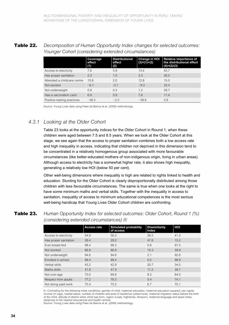
MULTIDIMENSIONAL POVERTY AND INEQUALITY OF OPPORTUNITY IN PERU: TAKING ADVANTAGE OF THE LONGITUDINAL DIMENSION OF YOUNG LIVES
34
Table 22. Decomposition of Human Opportunity Index changes for selected outcomes: Younger Cohort (considering extended circumstances)
Coverage effect (1)
Distributional effect (2)
Change in HOI (3)=(1)+(2)
Relative importance of the distributional effect (4)=(2)/(3)
Access to electricity 7.6 5.9 13.4 43.7
Has proper sanitation 2.3 1.0 3.3 30.0
Attended a childcare centre 10.8 2.0 12.8 15.5
Not stunted −6.1 -3.1 −9.3 33.4
Not underweight 0.9 0.4 1.2 28.7
Has a vaccination card 6.9 0.9 7.8 11.4
Positive rearing practices −36.5 −2.3 −38.8 5.9
Source: Young Lives data using Paes de Barros et al. (2009) methodology.
4.3.1 Looking at the Older Cohort
Table 23 looks at the opportunity indices for the Older Cohort in Round 1, when these
children were aged between 7.5 and 8.5 years. When we look at the Older Cohort at this stage, we see again that the access to proper sanitation combines both a low access rate
and high inequality in access, indicating that children not deprived in this dimension tend to be concentrated in a relatively homogenous group associated with more favourable circumstances (like better-educated mothers of non-indigenous origin, living in urban areas).
Although access to electricity has a somewhat higher rate, it also shows high inequality, generating a relatively low HOI (below 50 per cent).
Other well-being dimensions where inequality is high are related to rights linked to health and
education. Stunting for the Older Cohort is clearly disproportionally distributed among those
children with less favourable circumstances. The same is true when one looks at the right to have some minimum maths and verbal skills. Together with the inequality in access to sanitation, inequality of access to minimum educational competences is the most serious
well-being handicap that Young Lives Older Cohort children are confronting.
Table 23. Human Opportunity Index for selected outcomes: Older Cohort, Round 1 (%) (considering extended circumstances) II/
Access rate Simulated probability of access
Dissimilarity index
HOI
Access to electricity 54.9 56.2 26.5 41.3
Has proper sanitation 28.4 29.2 47.8 15.2
Ever breast-fed 98.4 98.3 0.8 97.5
Not stunted 66.8 66.8 10.3 59.9
Not underweight 94.6 94.6 2.1 92.6
Enrolled in school 99.4 99.4 0.5 98.9
Verbal skills 43.2 42.9 20.7 34.0
Maths skills 47.8 47.9 17.2 39.7
Not over-age 70.0 69.8 8.3 64.0
Respect from adults 77.2 78.3 5.4 74.1
Not doing paid work 75.4 75.2 6.7 70.1
II/. Controlling for the following initial conditions: gender of child, maternal education, maternal education squared, per capita income (in logs), marital status, number of children and area of residence (urban/rural), maternal migration status before the birth of the child, altitude of district when child was born, region (coast, highlands, Amazon), maternal language and asset index, distances to the nearest educational and health centres. Source: Young Lives data using Paes de Barros et al. (2009) methodology.

MULTIDIMENSIONAL POVERTY AND INEQUALITY OF OPPORTUNITY IN PERU: TAKING ADVANTAGE OF THE LONGITUDINAL DIMENSION OF YOUNG LIVES
35
Table 24 shows the opportunity indices in Round 2, when these children were between 11.5
and 12.5 years of age. Here we have added the standardised vocabulary test (PPVT) to evaluate their cognitive abilities. Again, low coverage of this ability and high inequities
combine to generate the lowest opportunity index.
Table 24. Decomposition of Human Opportunity Index changes for selected outcomes: Older Cohort, Round 2 (%) (considering extended circumstances) III/
Access rate Simulated probability of access
Dissimilarity index
HOI
Access to electricity 64.8 66.3 17.7 54.6
Has proper sanitation 32.9 35.0 37.8 21.8
Consumed proteins in last 24h 80.7 84.8 6.8 79.0
Not stunted 58.2 59.2 13.9 51.0
Enrolled in school 99.0 98.9 0.9 98.1
Not over-age 76.0 76.2 8.5 69.7
Verbal skills 79.6 79.5 6.9 74.0
Maths skills 93.4 93.7 3.0 90.8
High cognitive ability (standardised PPVT)
27.8 27.6 36.0 17.7
Respect from adults R2 91.5 95.8 2.1 93.8
Not doing paid work 69.0 69.0 7.2 64.1
III/. Controlling for the following initial conditions: gender of child, maternal education, maternal education squared, per capita income (in logs), marital status, number of children and area of residence (urban/rural), maternal migration status before the birth of the child, altitude of district when child was born, region (coast, highlands, Amazon), maternal language and asset index, distances to the nearest educational and health centres. Source: Young Lives data using Paes de Barros et al. (2009) methodology.
To achieve a larger increase in the opportunity index, expansions in coverage must be
accompanied by reductions in inequality of opportunity. As can be seen in Table 25, the largest ‘improvements’ in inequality have occurred in access to verbal and maths skills. However, this change is misleading as the relevance of the minimum cognitive skill depends
on age. The fact that 20 per cent of the sample still cannot read an extremely basic sentence years after the competence is expected cannot be considered a real improvement.17
17 The reading items required the children to read three letters (N, A, P); one word (‘pan’, which is Spanish for ‘bread’); and one sentence (‘El pan es rico’, which is Spanish for ‘the bread is delicious’). The item used to for writing assessment required
children to write the sentence ‘me gustan los perros’ (which is Spanish for ‘I like dogs’).

MULTIDIMENSIONAL POVERTY AND INEQUALITY OF OPPORTUNITY IN PERU: TAKING ADVANTAGE OF THE LONGITUDINAL DIMENSION OF YOUNG LIVES
36
Table 25. Decomposition of Human Opportunity Index for selected outcomes: Older Cohort (%) (considering extended circumstances)
Change in coverage effect (1)
Distributional effect (2)
Change in HOI (3)=(1)+(2)
Relative importance of the distributional effect(4)=(2)/(3)
Access to electricity 7.4 5.8 13.3 43.9
Has proper sanitation 3.0 3.5 6.5 53.4
Not stunted −6.8 −2.1 −8.9 23.9
Enrolled in school −0.5 −0.4 −0.9 47.0
Verbal skills 29.0 11.0 40.1 27.4
Maths skills 37.9 13.3 51.2 26.0
Not being over-age 5.9 −0.1 5.7 –
Respect from adults 16.6 3.2 19.7 16.0
Not doing paid work −5.8 −0.3 −6.0 4.8
Source: Young Lives data using Paes de Barros et al. (2008) methodology.
Inequality of opportunity may change when we redefine key outcomes considering issues of
quality. As can be seen in Table 26, as we move to more precise outcome definitions in
which the quality of the services is more closely monitored, then inequality of opportunity, as measured by the HOI increases. Here, although access to electricity is almost universal, when we take into account the number of hours households in the Young Lives sample have
access to this service, inequality increases dramatically. Similar results can be shown when we look at access to safe water.
Table 26. Changes in Human Opportunity Index along quality dimensions: Younger Cohort (%)
Coverage rate Dissimilarity Index
HOI
Electricity (Round 1)
Some access to electricity 96.84 1.29 95.59
Electricity all days (last 15 days) 70.25 9.17 63.81
Electricity 24 hours 58.34 14.55 49.86
Safe water (Round 2)
Access to piped water into dwelling 59.12 11.70 52.20
Access 7 days a week 47.71 11.31 42.31
Access 24 hours 21.45 15.27 18.17
Source: Escobal et al. 2009, based on Peru Young Lives data.

MULTIDIMENSIONAL POVERTY AND INEQUALITY OF OPPORTUNITY IN PERU: TAKING ADVANTAGE OF THE LONGITUDINAL DIMENSION OF YOUNG LIVES
37
6. Concluding remarks We have used Young Lives longitudinal data for Peru to construct a variety of indicators to
trace inequality of opportunity among children. First, we use aggregate indicators of
multidimensional poverty and different indices of deprivations that have the benefit of allowing for exact decomposition in both the well-being and the circumstance dimensions. Next we use the methodology developed in Paes de Barros et al. (2009) to measure an
opportunity index that aims to combine access to services and rights with the inequality of access, controlling for those circumstances that are beyond children’s control.
An important finding here is that independently of the index and the poverty threshold used,
the ranking of multidimensional poverty, deprivation, and lack of opportunities is the same when we group the children in alternative groupings based on their circumstances at birth:
mother’s indigenous origin, maternal education, area of residence (urban/rural), living at altitudes higher than 2,500 metres above sea level, remoteness, etc. It is precisely the groups of children in society that have less favourable circumstances who not only have less
access to basic services and other key well-being dimensions (like not being stunted, not having over-age, or being respected by adults), but are also the ones who are lagging behind as the public sector assigns disproportionally more resources to those children that lack one
or two of these opportunities (or have one or more of these deprivations) rather than address the lack of services and access to rights of those that are simultaneously deprived in many dimensions.
The paper has also shown that the ‘devil is in the detail’ as more precise definitions of certain
outcomes (for example, moving from access to a certain service to the number of hours in which the service is available to Young Lives families) can reveal hidden inequalities.
The paper shows that while there is an appearance of decreasing inequality according to
some indicators, this masks increasing inequality in other areas, and in particular that certain vulnerable groups may be left out of attempts to reduce inequality of opportunity across the
population. It also shows that although scalar indices of poverty, deprivations or inequality of opportunity may be useful as an advocacy tool, they may mask important heterogeneities so as to make such indicators, to say the least, insufficient to show the full scope and depth of
inequality of opportunity. Looking at a broader range of indicators, evaluating how opportunities and deprivations are unevenly distributed among children, and showing that circumstances are correlated is critical. So we need to look not just at opportunities or
deprivations between those that are affected by a certain circumstance and those that are not affected, but look at these indicators within groups of children affected simultaneously by a range of circumstances. This range of circumstances may be related to broader patterns of
discrimination and not just be related to specific and isolated circumstances.18
Trying to assess who is deprived in which dimensions requires being able to decompose
these indicators on both the circumstance dimension and the well-being dimension. This is something that the MPI does and into which it has provided some useful insights. Still, we
need to ask the broader question: it is really needed to aggregate multiple dimensions of child well-being in one unique indicator if we recognise that child well-being is truly
18 The distinction is related to the differences between horizontal and vertical inequality (Stewart et al. 2005).

MULTIDIMENSIONAL POVERTY AND INEQUALITY OF OPPORTUNITY IN PERU: TAKING ADVANTAGE OF THE LONGITUDINAL DIMENSION OF YOUNG LIVES
38
multidimensional and the well-being dimensions relevant at different stages in life are not the same. Is the pressure for a ‘simple’ unique indicator aimed at advocacy so high that we are willing to ignore this? Many UNICEF national reports construct aggregate indices based on
principal component analysis or other multivariate statistical techniques.
The MPI recognises that it is important to be explicit not only about the threshold from which
a deprivation is recognised, but also about mildness or severity in terms of a second threshold that indicates whether a child is deprived in just one dimension or is deprived many
dimensions. Although the MPI is a step forward in multidimensional poverty estimation, because its decomposability properties allow us to look at the relative importance of specific circumstances and the relative importance of specific well-being dimensions, it still fails to
provide a comprehensive account of multidimensional child poverty. If we want to pursue a better understanding of child poverty, we need not a single indicator but a range of indicators.
The pressure to look at just one gauge is nevertheless very strong, because of its supposed
simplicity. Many have argued that aggregate well-being indicators tend to be highly
correlated with GDP per capita and monetary poverty at the level of spatial aggregation where they are commonly used. This may be the result of mechanical aggregation, using only the indicators that are at hand (which typically favour material well-being), arbitrary
weights, or statistical procedures like principal component or factor analysis, which act as ‘grinders’, losing any relationship between weights and the intrinsic importance of the indicators for child well-being. Even worse, after pulling together everything, the index is
elevated to the category of a multidimensional index without its compilers knowing what it is really trying to aggregate.
On the other hand, the suggested aggregation techniques typically indicate that the one
should not use well-being dimensions that are highly correlated which each other (UNDP 2007: 22). Although this may be reasonable from the statistical point of view, it is very risky to
drop certain dimensions ‘just’ because they are highly correlated with others without understanding the intrinsic relationship between these dimensions, and which roles they play in understanding multidimensional child well-being.
Because of these considerations our opinion is that either one should not try to aggregate
dimensions that are by nature different, or one should be much more explicit about the trade-offs one is prepared to admit in relation to this. If absolutely necessary, aggregation could be done in either of two ways. One is obtaining a consensus regarding the relative importance
that society places on different child well-being dimensions. This may be called a normative aggregation. The other way is to find what implicit trade-off exists, regardless of normative considerations. For example, we can use the amount of resources that are allocated in the
national budget for each dimension and for each social sub-group as a way of recognising the implicit trade-offs. Even in this case, it is very likely that both indicators would be needed.
Aggregate multidimensional poverty indices are here to stay, whether we like them or not.
This paper has shown that although scalar indices of poverty, deprivations or inequality of
opportunity may be somewhat useful as an advocacy tool (as the poverty rankings between those having different circumstances may be reasonably robust), they may mask important heterogeneities, which makes them of limited usefulness for analytical and policy purposes,
once we move beyond counting poor children.
One further area of concern which has not been directly addressed in this paper is the unit of
analysis on which many of these indicators are based. In our own case we are taking advantage of child-specific data that has been collected at an individual level and using a

MULTIDIMENSIONAL POVERTY AND INEQUALITY OF OPPORTUNITY IN PERU: TAKING ADVANTAGE OF THE LONGITUDINAL DIMENSION OF YOUNG LIVES
39
longitudinal framework. However, statistical agencies and international organisations (like UNICEF and UNDP) are forced to construct their indices using already aggregated data at the sub-national or national level. Further analysis is urgently needed to understand the
potential biases that these alternative aggregation schemes generate, once we lose contact with the multidimensional nature of each child and allow that at the aggregate level 50 per cent of boys and girls with a certain deprivation is not different from 100 per cent of girls with
a deprivation and no boy deprived; or that changes in individual multidimensional poverty do not matter as long as the aggregate remains the same.
We have shown the complexity of child poverty, and how misleading it can be to rely on a
single multidimensional measure of poverty. However complex and sophisticated the
measure may be, it cannot show all the variations in outcomes. On the other hand, dimensions of deprivations cannot be understood without relating them to each other. A multi-dimensional approach is necessary, but this should not be in the form of a single
multidimensional measure. We cannot rely solely on aggregate measures of poverty if support is to be given to the most disadvantaged groups of children.

MULTIDIMENSIONAL POVERTY AND INEQUALITY OF OPPORTUNITY IN PERU: TAKING ADVANTAGE OF THE LONGITUDINAL DIMENSION OF YOUNG LIVES
40
References Alkire, S. and J. Foster (2008) Counting and Multidimensional Poverty Measurement, OPHI
Working Paper No.7 (revised May 2008), Oxford: Oxford Poverty and Human Development
Initiative (OPHI), University of Oxford
Barrón, M. (2008) ‘Exclusion and Discrimination as Sources of Inter-ethnic Inequality in
Peru’, Economia 31.61: 51–80
Bourguignon, F. and S.R. Chakravarty (2003) ‘The Measurement of Multidimensional
Poverty’, Journal of Economic Inequality 1.1: 25–49
Bourguignon, F., F. Ferreira and M. Menendez (2003) Inequality of Outcomes and Inequality
of Opportunities in Brazil, Policy Research Working Paper No. 3174, World Bank, Washington DC
Chakravarty, S.R., D. Mukherjee and R. Ranade (1998) ‘On the Family of Subgroup and
Factor Decomposable Measures of Multidimensional Poverty’, Research on Economic Inequality 8: 175–194
Cueto, S., J. Leon, G. Guerrero and I. Muñoz (2009) Psychometric Characteristics of
Cognitive Development and Achievement Instruments in Round 2 of Young Lives, Technical
Note 15, Oxford: Young Lives
Cueto, S. (2005) ‘Height, Weight, and Educational Achievement in Rural Peru’, Food and
Nutrition Bulletin 26.2: S251–S260
Elbers, C., P. Lanjouw , J.A. Mistiaen and Berk Özler (2008) ‘Reinterpreting Between-group
Inequality’, Journal of Economic Inequality 6.3: 231–245
Engle, P.L., P. Menon and L. Haddad (1999) ‘Care and Nutrition: Concepts and
Measurement’, World Development 27.8: 1309–37
Escobal, J., J. Saavedra and R. Vakis (2012) ‘¿Está el Piso Parejo para los Niños en el Perú? Medición y Comprensión de la Evolución de las Oportunidades’, Lima: World Bank
and Grupo de Análisis para el Desarollo (GRADE)
Escobal, J. and C. Ponce (2010) ‘Dinámicas Provinciales de Pobreza en el Perú 1993–
2007’, Working Paper, Santiago de Chile: Programa Dinámicas Territoriales Rurales Rimisp – Centro Latinoamericano para el Desarrollo Rural
Escobal, J. and E. Flores (2009): Maternal Migration and Child Well-being in Peru, Working Paper 56. Oxford: Young Lives
Escobal, J., P. Ames, S. Cueto, M. Penny and E. Flores (2008) ‘Young Lives Round 2
Survey: Initial Report for Peru’, Oxford: Young Lives
Escobal, J. and E. Flores (2008) An Assessment of the Young Lives Sampling Approach in
Peru, Technical Note 3, Oxford: Young Lives
Ferreira, F. and J. Gignoux (2008) The Measurement of Inequality of Opportunity: Theory
and an Application to Latin America, Policy Research Working Paper No. 4659, Washington DC: World Bank

MULTIDIMENSIONAL POVERTY AND INEQUALITY OF OPPORTUNITY IN PERU: TAKING ADVANTAGE OF THE LONGITUDINAL DIMENSION OF YOUNG LIVES
41
Figueroa. A. and M. Barrón (2005) Inequality, Ethnicity and Social Disorder in Peru, Working
Paper 8, Oxford: Centre for Research on Inequality, Human Security and Ethnicity (CRISE), University of Oxford
Foster, J.E., J. Greer and E. Thorbecke (1984) ‘A Class of Decomposable Poverty
Measures’, Econometrica 52.3: 761–5
Gordon D., S. Nandy, C. Pantazis, S. Pemberton and P. Townsend (2003) Child Poverty in
the Developing World, Bristol: Policy Press
INEI (2010) ‘Indicadores del Programa Articulado Nutricional’,
http://www1.inei.gob.pe/biblioineipub/bancopub/Est/Lib0859 (accessed March 2011)
Jaramillo, M. and J. Saavedra (2009) ‘Inequality in Post-Structural Reform Peru: The Role of
Market Forces and Public Policy’ in UNDP, The New Dynamics of Inequality in Latin
America, Washington DC: Brookings Institution Press
Kovacevic, M. (2010) Measurement of Inequality in Human Development – A Review,
Human Development Research Paper 2010/35, New York: UNDP
Lefranc, A., N. Pistolesi and A. Trannoy (2006) Inequality of Opportunities vs. Inequality of
Outcomes: Are Western Societies All Alike?, ECINEQ Discussion Paper No. 2006-54, Palma de Mallorca: Society for the Study of Economic Inequality
Lopez-Calva, L. and N. Lustig (2009) The Recent Decline of Inequality in Latin America:
Argentina, Brazil, Mexico and Peru, Working Paper No. 140, Palma de Mallorca: Society for the Study of Economic Inequality
Lynch, S.M. (2003) ‘Cohort and Life-Course Patterns in the Relationship Between Education
and Health: A Hierarchical Approach’, Demography 40.2: 309–31
Muñoz, I., M. Paredes and R. Thorp (2007): ‘Group Inequalities and the Nature and Power of
Collective Action: Case Studies from Peru’ in World Development 35.11: 1929–46
Nardo, M., M. Saisana, A. Saltelli, S. Tarantola, A. Hoffman and E. Giovannini (2005)
Handbook on Constructing Composite Indicators: Methodology and User Guide, OECD Statistics Working Paper, Paris: OECD
Outes-Leon, I. and S. Dercon (2007) Survey Attrition and Attrition Bias in the Young Lives
Study, Technical Note 5, Oxford: Young Lives
Paes de Barros, R., F. Ferreira, J. Molinas and J. Saavedra (2009) Measuring Inequality of
Opportunities in Latin America and the Caribbean, Washington DC: World Bank
Roemer, J.E. (1998) Equality of Opportunity, Cambridge, MA: Harvard University Press
Ruiz-Castillo, J. (2003) ‘The Measurement of Inequality of Opportunities’ in J. Bishop and Y. Amiel (eds) Research in Economic Inequality 9: 1–34
Sen, A. (1985) Commodities and Capabilities, Amsterdam: North Holland
Sen, A. (1976) ‘Poverty: An Ordinal Approach to Measurement’, Econometrica 44.2: 219–31
Stewart, F., G. Brown and L. Mancini (2005) Why Horizontal Inequalities Matter: Some
Implications for Measurement, Working Paper 19, Oxford: Centre for Research on Inequality,
Human Security and Ethnicity (CRISE), University of Oxford
Strauss, J. and D. Thomas (2007) ‘Health over the Life Course’ in T. Paul Schultz and John
Strauss (eds) Handbook of Development Economics Vol. 4, Amsterdam: North Holland

MULTIDIMENSIONAL POVERTY AND INEQUALITY OF OPPORTUNITY IN PERU: TAKING ADVANTAGE OF THE LONGITUDINAL DIMENSION OF YOUNG LIVES
42
UNICEF (2007) Poverty and Children: A Perspective, New York: UNICEF
UNDP (2007) ‘Measuring Human Development: A Primer. Guidelines and Tools for
Statistical Research, Analysis and Advocacy’, New York: UNICEF

MULTIDIMENSIONAL POVERTY AND INEQUALITY OF OPPORTUNITY IN PERU: TAKING ADVANTAGE OF THE LONGITUDINAL DIMENSION OF YOUNG LIVES
43
Statistical Appendix Table A1. Multidimensional well-being in key sub-groups (first grouping, showing
indicators): Younger Cohort (%) Indigenous
language
4 or more siblings
Low maternal education
Indigenous language
3 or fewer siblings
Medium maternal education
Non-indigenous language
3 or fewer siblings
Low maternal education
Low/medium income
Non-indigenous language
3 or fewer siblings
Medium maternal education
Low/medium income
Non-indigenous language
3 or fewer siblings
Medium maternal education
High income
Non-indigenous language
3 or fewer siblings
High maternal education
Medium/high income
Low altitude area
Odds of being poor between the worst and best backgrounds
Round 1
Access to electricity 37.1 42.3 39.6 56.2 82.4 90.9 6.9
Has proper sanitation 9.7 23.8 16.7 30.4 63.9 73.2 3.4
Adequate weight at birth 92.4 96.4 98.4 91.4 93.1 95.8 1.8
Pre-natal care 90.0 96.3 91.4 88.1 96.5 98.3 5.9
Attended a childcare centre 4.6 4.3 1.5 1.4 4.6 6.6 1.0
Not stunted 42.3 57.7 71.2 75.0 84.2 87.5 4.6
Not underweight 82.8 92.4 87.3 94.2 94.1 98.2 9.8
Has a vaccination card 82.5 85.8 95.2 91.9 86.7 91.7 2.1
Positive rearing practices 55.8 63.2 70.5 66.1 76.1 80.1 2.2
Round 2
Access to electricity 47.5 51.0 71.3 71.3 90.9 94.7 9.9
Access to safe drinking water 69.7 76.4 71.2 68.0 88.5 90.9 3.3
Has proper sanitation 7.4 21.0 16.9 37.1 70.3 79.2 4.5
Not stunted 33.5 47.0 61.3 62.1 81.4 88.1 5.6
Not underweight 88.3 94.4 88.2 94.2 96.0 99.0 11.5
Attended a childcare centre 21.3 20.1 2.2 10.2 20.4 27.5 1.1
Pre-school enrolment 63.8 80.3 72.1 79.5 88.9 96.3 9.8
Has a vaccination card 96.7 97.4 95.6 96.6 96.3 97.9 1.6
Consumed protein in last 24h 84.3 93.0 91.6 87.9 95.8 99.0 15.6
Positive rearing practices 35.0 48.0 25.8 28.1 27.3 21.2 0.8
High cognitive ability (standardised PPVT)
7.5 15.9 13.2 20.5 39.4 59.2 2.3
Note: Indicators are based in the Panel sub-sample.

MULTIDIMENSIONAL POVERTY AND INEQUALITY OF OPPORTUNITY IN PERU: TAKING ADVANTAGE OF THE LONGITUDINAL DIMENSION OF YOUNG LIVES
44
Table A2. Multidimensional well-being in key sub-groups (second grouping, showing indicators): Younger Cohort (%)
Indigenous language
Low maternal education
Indigenous language
Medium maternal education
Indigenous language
High maternal education
Non-indigenous language
3 or fewer siblings
Low/ medium maternal education
Low income
Non-indigenous language
3 or fewer siblings
Low/ medium maternal education
Medium income
Non-indigenous language
3 or fewer siblings
Low/ medium maternal education
High income
Non-indigenous language
3 or fewer siblings
High maternal education
Low income
Non-indigenous language
3 or fewer siblings
High maternal education
Medium income
Non-indigenous language
3 or fewer siblings
High maternal education
High income
Non-indigenous language
4 or more siblings
Low/ medium maternal education
Non-indigenous language
4 or more siblings
High maternal education
Odds of being poor between the worst and best back-grounds
Round 1
Access to electricity 29.4 48.7 77.7 42.6 62.0 79.8 65.3 87.7 93.0 46.7 86.3 1.5
Has proper sanitation
6.6 24.9 46.9 24.0 34.2 61.2 47.3 63.8 79.3 23.8 62.8 1.0
Adequate weight at birth
94.3 97.1 91.4 92.0 92.1 93.5 96.6 94.3 96.8 90.3 97.8 3.0
Pre-natal care 93.7 94.2 89.2 80.6 92.6 96.2 98.8 98.3 98.3 84.0 91.6 0.4
Attended childcare centre
3.3 3.7 2.6 3.3 1.4 5.1 2.3 6.8 6.4 2.4 4.0 1.0
Not stunted 46.0 58.9 78.4 71.9 74.1 84.1 82.0 83.4 90.1 61.6 85.0 1.1
Not underweight 86.8 93.1 97.4 94.5 91.5 95.3 97.3 98.0 98.4 90.1 97.7 2.1
Has vaccination card
89.2 85.8 80.1 92.9 88.8 87.6 93.9 92.1 91.4 89.8 85.9 0.9
Positive rearing practices
58.2 64.6 68.2 58.4 71.4 76.1 67.9 79.5 80.6 71.5 84.0 1.5
Round 2
Access to electricity 43.9 56.6 86.7 64.4 77.4 89.3 78.3 93.9 95.2 55.1 92.1 1.4
Access to safe drinking water
69.9 75.0 78.8 56.9 76.1 87.5 84.7 89.7 91.6 56.5 89.9 1.2
Has proper sanitation
7.6 22.9 55.1 28.3 39.6 67.3 51.7 70.4 84.9 29.0 74.5 1.3
Not stunted 35.9 46.9 74.4 56.3 65.2 80.0 77.1 82.3 91.9 54.4 80.6 1.0
Not underweight 89.0 94.0 98.7 93.2 92.8 94.9 95.9 98.6 99.2 94.3 97.9 2.5
Attended a childcare centre
24.1 17.4 20.7 7.1 11.6 20.5 11.0 28.9 26.5 10.6 24.3 1.1
Pre-school enrolment
69.6 77.7 82.3 76.4 80.3 87.7 94.5 92.7 98.6 74.6 95.1 2.5
Has a vaccination card
97.1 98.0 92.3 95.9 96.1 97.0 98.7 96.6 98.7 97.1 97.9 1.4
Consumed protein in past 24h
85.9 92.3 98.5 84.4 92.3 95.4 94.4 98.4 99.4 82.5 100.0
Positive rearing practices
38.9 48.3 43.5 26.6 29.4 26.2 25.8 25.6 18.4 31.3 20.5 0.9
High cognitive ability (standardised PPVT)
7.0 16.0 44.3 14.3 22.7 36.8 44.0 48.7 66.0 12.1 42.2 1.1
Note: Indicators are based in the Panel sub-sample.

MULTIDIMENSIONAL POVERTY AND INEQUALITY OF OPPORTUNITY IN PERU: TAKING ADVANTAGE OF THE LONGITUDINAL DIMENSION OF YOUNG LIVES
45
Table A3. Multidimensional well-being in key sub-groups (first grouping, by different definitions): Younger Cohort (%)
Indigenous language
4 or more siblings
Low maternal education
Indigenous language
3 or fewer siblings
Medium maternal education
Non-indigenous language
3 or fewer siblings
Low maternal education
Low/medium income
Non-indigenous language
3 or fewer siblings
Medium maternal education
Low/medium income
Non-indigenous language
3 or fewer siblings
Medium maternal education
High income
Non-indigenous language
3 or fewer siblings
High maternal education
Medium/high income
Low altitude area
Round 1
Union 97.5 90.2 92.8 85.2 63.9 53.3
Intersection 0.6 0.0 0.0 0.0 0.0 0.0
Chakravarty (α=0) 41.4 33.6 31.4 26.6 16.1 11.2
Chakravarty (α=1) 26.0 23.9 23.2 20.6 11.7 8.6
Chakravarty (α=2) 34.5 27.8 26.8 23.3 13.9 9.5
Round 2
Union 98.6 95.3 98.6 94.8 85.5 86.9
Intersection 0.6 0.0 0.0 0.0 0.0 0.0
Chakravarty (α=0) 41.6 34.5 34.4 30.1 19.7 17.1
Chakravarty (α=1) 26.1 23.3 24.4 21.8 15.6 14.8
Chakravarty (α=2) 33.4 27.5 28.7 25.1 16.9 15.5
Note: Indicators are based in the Panel sub-sample. Source: Young Lives data using Bourguignon and Chakravarty (2003) and Chakravarty et al. (1998) methodology.
Table A4. Multidimensional poverty in key sub-groups (second grouping, by different definitions): Younger Cohort (%)
Indigenous language
Low maternal education
Indigenous language
Medium maternal education
Indigenous language
High maternal education
Non-indigenous language
3 or fewer siblings
Low/med.maternal education
Low income
Non-indigenous language
3 or fewer siblings
Low/med. maternal education
Medium income
Non-indigenous language
3 or fewer siblings
Low/med. maternal education
High income
Non-indigenous language
3 or fewer siblings
High maternal education
Low income
Non-indigenous language
3 or fewer siblings
High maternal education
Medium income
Non-indigenous language
3 or fewer siblings
High maternal education
High income
Non-indigenous language
4 or more siblings
Low/med. maternal education
Non-indigenous language
4 or more siblings
High maternal education
Round 1
Union 98.7 90.0 75.4 89.2 85.7 66.4 74.5 63.2 47.2 90.5 56.4
Intersection 0.5 0.0 0.0 0.0 0.0 0.0 0.0 0.0 0.0 0.8 0.0
Chakravarty α=0 40.9 32.1 21.6 31.3 25.4 16.5 22.1 13.8 9.7 31.8 14.0
Chakravarty α=1 26.6 22.7 16.8 24.5 18.7 12.4 17.9 10.2 7.5 21.6 10.8
Chakravarty α=2 34.6 26.5 19.1 27.7 21.7 14.4 19.9 11.6 8.3 28.0 11.9
Round 2
Union 98.2 94.3 82.2 95.6 94.9 86.6 92.3 86.5 86.8 94.2 91.7
Intersection 0.5 0.0 0.0 0.0 0.0 0.0 0.0 0.0 0.0 0.0 0.0
Chakravarty α=0 41.2 33.3 21.3 33.8 28.6 20.9 25.1 19.0 15.8 34.9 19.5
Chakravarty α=1 26.0 21.9 16.8 24.0 21.0 16.6 19.9 15.4 14.3 24.1 15.8
Chakravarty α=2 34.1 27.6 17.7 28.6 23.5 17.7 21.7 16.5 14.8 29.4 16.6
Note: Indicators are based in the Panel sub-sample. Source: Young Lives data using Bourguignon and Chakravarty (2003) and Chakravarty et al. (1998) methodology.

MULTIDIMENSIONAL POVERTY AND INEQUALITY OF OPPORTUNITY IN PERU: TAKING ADVANTAGE OF THE LONGITUDINAL DIMENSION OF YOUNG LIVES
46
Table A5. Human Opportunity Index for selected outcomes: Younger Cohort, Round 2 (%) (considering basic circumstances) I/
Access rate Simulated probability of access
Dissimilarity Index
Human Opportunity Index (HOI)
Access to electricity 69.9 70.1 16.6 58.5
Has proper sanitation 42.0 42.1 35.0 27.4
Not stunted 62.6 63.0 15.2 53.4
Not underweight 94.1 94.2 1.9 92.4
Attended childcare centre 19.5 19.7 14.6 16.9
Pre-school enrolment 81.5 81.4 6.7 75.9
Has vaccination card 97.0 97.1 0.6 96.6
Consumed protein in last 24h 91.3 91.3 3.5 88.2
Positive rearing practices 31.2 31.0 8.2 28.5
I/. Controlling for the following initial conditions: gender of child, maternal education, maternal education squared, per capita income (in logs), marital status, number of children and area of residence (urban/rural). Source: Young Live data using Paes de Barros et al. (2009) methodology.
Table A6. Human Opportunity Index for selected outcomes: Older Cohort, Round 1 (%) (considering basic circumstances) I/
Access rate Simulated probability of access
Dissimilarity Index
Human Opportunity Index (HOI)
Access to electricity 54.3 54.1 28.3 38.8
Has proper sanitation 28.7 28.2 47.6 14.8
Ever breastfed 98.1 98.5 0.6 97.8
Not stunted 65.4 65.3 11.1 58.0
Not underweight 93.9 94.1 1.4 92.8
Enrolled in school 99.2 99.4 0.3 99.1
Not over-age 69.3 69.7 8.2 64.0
Respect from adults 76.7 76.8 5.3 72.7
Not doing paid work 76.1 75.9 6.1 71.3
I/. Controlling for the following initial conditions: gender of child, maternal education, maternal education squared, per capita income (in logs), marital status, number of children and area of residence (urban/rural). Source: Young Lives data using Paes de Barros et al. (2009) methodology.

MULTIDIMENSIONAL POVERTY AND INEQUALITY OF OPPORTUNITY IN PERU: TAKING ADVANTAGE OF THE LONGITUDINAL DIMENSION OF YOUNG LIVES
47
Table A7. Human Opportunity Index for selected outcomes: Older Cohort, Round 2 (%) (considering basic circumstances) I/
Access rate Simulated probability of access
Dissimilarity Index
Human Opportunity Index (HOI)
Access to electricity 64.8 65.1 20.6 51.7
Has proper sanitation 32.9 34.0 42.2 19.6
Consumed protein in last 24h 80.7 83.8 6.3 78.5
Not stunted 58.2 59.7 12.9 52.0
Enrolled in school 99.0 99.1 0.5 98.6
Not over-age 76.0 77.6 7.2 72.0
Respect from adults 91.5 95.1 2.1 93.1
Not doing paid work 69.0 70.6 5.9 66.4
I /. Controlling for the following initial conditions: gender of child, maternal education, maternal education squared, per capita income (in logs), marital status, number of children and area of residence (urban/rural). Source: Young Lives data using Paes de Barros et al. (2009) methodology.


Young Lives is an innovative long-term international research project investigating the changing nature of childhood poverty.
The project seeks to:
• improveunderstandingof thecausesandconsequencesof childhood povertyandtoexaminehowpoliciesaffectchildren’swell-being
• informthedevelopmentandimplementationof futurepoliciesandpracticesthatwillreducechildhoodpoverty.
YoungLivesistrackingthedevelopmentof 12,000childreninEthiopia, India(AndhraPradesh),PeruandVietnamthroughquantitativeandqualitativeresearchovera15-yearperiod.
Young Lives Partners
YoungLivesiscoordinatedbyasmallteambasedattheUniversityof Oxford, ledbyJoBoyden.
EthiopianDevelopmentResearchInstitute,Ethiopia
CentreforEconomicandSocialSciences, AndhraPradesh,India
SavetheChildren–BalRakshaBharat,India
SriPadmavathiMahilaVisvavidyalayam(Women’sUniversity),AndhraPradesh,India
GrupodeAnálisisparaelDesarollo (GroupfortheAnalysisofDevelopment),Peru
InstitutodeInvestigaciónNutricional (InstituteforNutritionalResearch),Peru
CentreforAnalysisandForecast, VietnameseAcademyofSocialSciences,Vietnam
GeneralStatisticsOffice,Vietnam
SavetheChildren,Vietnam
TheInstituteofEducation,UniversityofLondon,UK
ChildandYouthStudiesGroup(CREET),TheOpenUniversity,UK
DepartmentofInternationalDevelopment,UniversityofOxford,UK
SavetheChildrenUK (staffinthePolicyDepartmentinLondon andprogrammestaffinEthiopia).
YoungLives,OxfordDepartmentofInternationalDevelopment(ODID)
UniversityofOxford,QueenElizabethHouse3MansfieldRoad,OxfordOX13TB,UK
Tel:+44(0)1865281751 Fax:+44(0)1865281801
Email:[email protected]
www.younglives.org.uk