multidisciplinary design optimization of automotive ... · pdf filesubmitted to aiaa journal 1...
TRANSCRIPT

Submitted to AIAA Journal
1
MULTIDISCIPLINARY DESIGN OPTIMIZATION OF AUTOMOTIVE CRASHWORTHINESS AND NVH USING
RESPONSE SURFACE METHODS
K.J. Craig1,*, Nielen Stander2, D.A. Dooge3 and S. Varadappa4 1 Multidisciplinary Design Optimization Group (MDOG), Department of Mechanical
and Aeronautical Engineering, University of Pretoria, Pretoria 0002, South Africa [email protected]
2 Livermore Software Technology Corporation, 7374 Las Positas Rd, Livermore, CA 94550, USA
[email protected] 3Advanced Vehicle Engineering, DaimlerChrysler Corporation
800 Chrysler Drive East, Auburn Hills, MI 48326, USA [email protected]
4Quantum Consultants, Inc., East Lansing, USA * Professor. Currently on sabbatical leave at Livermore Software Technology Corporation.
Abstract This paper describes the multidisciplinary design optimization of a full vehicle to minimize mass while complying with crashworthiness and Noise, Vibration and Harshness (NVH) constraints. A full frontal impact is used for the crashworthiness simulation in the nonlinear dynamics code, LS-DYNA. The NVH constraints are evaluated from an implicit modal analysis of a body-in-white vehicle model using LS-DYNA. Seven design variables describe the structural components of which the thickness can be varied. The components are the aprons, shotguns, rails, cradle rails and the cradle cross member. The crashworthiness constraints relate to crush energy and displacement, while the torsional frequency characteristics are obtained from the modal analysis. The Multidisciplinary Feasible (Fully Integrated) formulation, in which full sharing of the variable sets is employed, is used as the reference case. In an attempt to investigate global optimality, three starting designs are used. Based on a Design of Experiments analysis of variance of the fully-shared variable results for each starting design, discipline-specific variables are selected from the full set using the sensitivity of the disciplinary responses. The optimizer used in all cases is the Successive Response Surface Method as implemented in LS-OPT. It is shown that partial sharing of the variables not only reduces the computational cost in finding an optimum due to fewer, more sensitive variables, but also leads to a better result. The mass of the vehicle is reduced by 4.7% when starting from an existing baseline design, and by 2.5% and 1.1% when starting from a lightest and heaviest starting design respectively. Keywords: Multidisciplinary Design Optimization, response surface methodology, crashworthiness, NVH, MDO formulations, design of experiments, mode tracking.
Submitted to AIAA Journal
2
Introduction Although still in its infancy, mathematical optimization techniques are increasingly being applied to the crashworthiness design of vehicles. Early crashworthiness studies of the mid 1980’s were followed by response surface-based design optimization studies in the 1990’s for occupant safety1,2, component-level optimization3-5, airbag-related parameter identification6 and for a full-vehicle simulation7-9. These studies focus on one single discipline in the simulation, that of the nonlinear dynamics of the crash event. There is increasing interest in the coupling of other disciplines into the optimization process, especially for complex engineering systems like aircraft and automobiles10. The aerospace industry was the first to embrace multidisciplinary design optimization (MDO)11-13, because of the complex integration of aerodynamics, structures, control and propulsion during the development of air- and spacecraft. The automobile industry has followed suit14-16. In Ref.14, the roof crush performance of a vehicle is coupled to its Noise, Vibration and Harshness (NVH) characteristics (modal frequency, static bending and torsion displacements) in a mass minimization study, while Ref.15 extends the study in Ref.14 to include other crash modes, i.e., full frontal and 50% frontal offset impact. Ref. 16 considers the impact of a bumper beam coupled with a bound on its first natural frequency. Different methods have been proposed when dealing with MDO. The conventional or standard approach is to evaluate all disciplines simultaneously in one integrated objective and constraint set by applying an optimizer to the multidisciplinary analysis (MDA), similar to that followed in single-discipline optimization. The standard method has been called multidisciplinary feasible (MDF), as it maintains feasibility with respect to the MDA, but, as it does not imply feasibility with respect to the disciplinary constraints, it has also been called fully integrated optimization (FIO)17,18. A number of MDO formulations are aimed at decomposing the MDF problem. Concentrating here on hierarchical or structural decomposition (for non-hierarchical including partitioning approaches refer to e.g. Ref.10 and Ref.19), the formulation usually consists of multiple levels. One notable approach, because of the way in which it matches organizational structures, is collaborative optimization (CO)20-23. Other multilevel approaches are: concurrent subspace optimization (CSSO)24, bi-level integrated systems synthesis (BLISS)25,26, optimization by a mix of dissimilar analysis and approximations (OMDAA)14 and optimization by linear decomposition (OLD)17. Another class of MDO formulations maintains the single level optimization of MDF, but distributes the analyses in different ways. Examples are simultaneous analysis and design (SAND)27, also called ‘All-at-once’21, and interdisciplinary feasible (IDF)28, also called distributed analysis optimization (DAO)18. Additional linking variables are introduced and treated through the addition of compatibility or consistency constraints at the system level. The choice of MDO formulation depends on the degree of coupling between the different disciplines and the ratio of shared to total design variables29. The framework of the formulation chosen has to comply with a number of requirements regarding the architecture, construction, information access and execution30. The objective function, i.e. the criterion that is minimized in crashworthiness optimization, and constraints on the optimization, have mostly been related to occupant safety. E.g. the Head Injury Criterion2 is used as objective in Refs.1, 15 and 31, while

Submitted to AIAA Journal
3
maximum knee force or a femur force-related criterion is used to drive the design optimization in Ref.5. Criteria related to other body parts are the Rib Deflection Criterion or Viscous Criterion (rib cage), the Abdomen Protection Criterion (abdominal area) and Pelvis Performance Criterion (pelvis area)3. Other objectives or constraints are related to structural integrity during a crash. Examples are intrusion kinematics (displacement, velocity or acceleration), and the crush history, e.g. in a multi-stage form of the acceleration versus displacement history. The selection depends on the design criteria and type of crash, e.g., side impact, full and partially offset frontal impact or roof crush. In an MDO sense, one would use an overall design objective as the objective function. An obvious choice is the total vehicle mass or the mass of the parts being designed, as it impacts positively on material cost, manufacturing cost and operating cost. The other candidates listed above would then enter the optimization problem as constraints to ensure a safe, lightweight vehicle. As far as design variables are concerned, these have mainly been geometrical in nature in crashworthiness studies. E.g., in Ref.2, airbag and seat belt variables are used, while in Ref.5, gages and radii of brackets and the yoke of a knee-bolster system are optimized. In Ref.12, the thickness and stiffness of a variety of vehicle subcomponents make up the 19 NVH-only, 10 crash-only and 10 discipline-shared design variables. In the current study, all of the variables relate to thickness or gage. As this is the first MDO study using LS-OPT, it has as its aim the provision of a benchmark for further studies. For this reason the MDF formulation is chosen in this paper. Comparison with other MDO formulations for a simpler test case vehicle is described in a companion paper31. The MDF formulation layout as customized for the current disciplines is shown in Figure 1. As the current study uses response surfaces in the optimization process, the different disciplines could have different experimental designs and partially shared design variables in general. E.g., if the NVH analysis also provides analytical sensitivities, only one experimental point is necessary, and a linear response surface can be constructed from the sensitivities or gradients. The construction of the response surfaces will be discussed in more detail in the Methodology section below.
Submitted to AIAA Journal
4
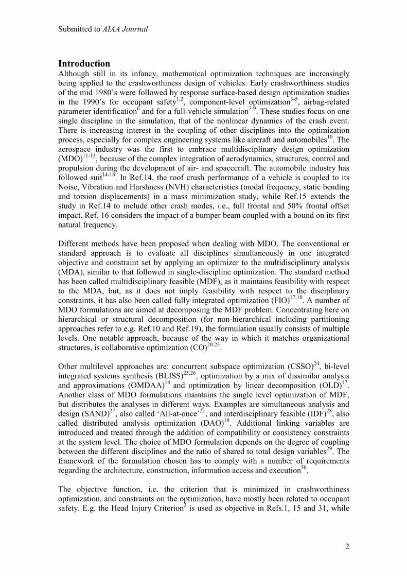
System-level Optimizer Goal: Minimize Mass s.t. Crashworthiness and NVH constraints
Multidisciplinary Analyses
Crashworthiness analysis
NVH analysis
State variables
Design variables
Figure 1 – Multidisciplinary feasible (MDF) MDO architecture
Methodology Optimization algorithm The following is a brief outline of the Successive Response Surface Method (SRSM) as implemented in LS-OPT32. This optimization algorithm uses a Response Surface Methodology (RSM)33, i.e., a Design of Experiments approach, to construct linear response surfaces on a subregion from a D-optimal subset of experiments. The D-optimality criterion is implemented using a genetic algorithm and a 50% over-sampling is typically used. Successive subproblems are solved using a multi-start variant of the leap-frog dynamic trajectory method, LFOPC34. The multi-start locations are generated using a Latin hypercube experimental design, and the best optimum is selected as the optimum of the subproblem. The size of successive subregions is adapted based on contraction and panning parameters designed to prevent oscillation and premature convergence35,36. Infeasibility is handled automatically when it occurs through the construction and solution of an auxiliary problem to bring the design within the subregion if possible. The method handles noisy responses automatically through the selection of an initially large subregion or range and a typically 50% over-sampling of experiments in the implementation of the D-Optimality criterion37. As the optimum is approached, the subregion is contracted automatically, implying that inaccuracies in the sensitivity information do not cause large departures from the previous design. Therefore this handling of the step-size dilemma38 also provides an inherent move limit to the algorithm. MDO modifications to LS-OPT32 When applying SRSM to MDF, discipline-specific experimental designs and variable sets are allowed. After each iteration, the variables that are not shared are updated to ensure a unique intermediate design and multidisciplinary feasibility.
Submitted to AIAA Journal
5
Variable screening As the MDO problem solution cost and coupling depends directly on the way in which variables are shared, a design of experiments (DOE) Analysis of Variance (ANOVA) study is performed using LS-OPT39 before the different variable sets are fixed for each discipline. During the successive RSM procedure, the variance of each variable with respect to each response fitted, is tracked and tested for significance using the partial F-test33 for each response. The importance of a variable is penalized by both a small absolute coefficient value (weight) computed from the regression, as well as by a large uncertainty in the value of the coefficient pertaining to the variable. A 90% confidence level is used to quantify the uncertainty and the variables are ranked based on this level. Since the relative importance of variables can vary as the optimization progresses through the design space, care should be taken not to screen variables prematurely. Non-linearity can affect ranking due to rapid changes of gradients as well as significant modeling error. Mode tracking In the NVH analyses below, it is required to control the frequencies of specific modes during the optimization. Because mode switching can occur, i.e. the sequence of a specific mode can trade places with another mode when sorted by frequency, obtaining the frequency of a specific mode cannot be performed through mode number alone. To track a specific mode, the following modification was made to LS-DYNA40, the finite element solver used in this study. The frequencies of the modes are obtained from a linear modal analysis. The eigenvalues, λ, are obtained from the solution of the linear system.41 φλφ MK = (1) where K is the stiffness and M the mass matrix. The associated eigenvectors, φ, describe the mode shape at each frequency, λ. During the optimization, the mode number associated with, say, the torsional frequency, may switch with another mode when the modes are sorted by frequency. This switch may be due to modifications to the design prescribed by the optimizer. When the frequency of a particular mode is included in the optimization problem formulation as either an objective or a constraint, it is therefore desirable to be able to track any mode switching automatically. In the current study, this is done by performing a scalar product of the mass-orthogonalized eigenvector ( ijj
Ti M δφφ = , δij being the Kronecker delta) associated with
the mode of interest in the baseline design, with each of the mass-orthogonalized eigenvectors of the modified design, and finding the maximum scalar product42. In this scalar product search, the eigenvectors are weighted by the diagonal of the mass matrix in the following fashion:
( ) ( )
jj
T
jMM φφ 2
121
00max (2)
Submitted to AIAA Journal
6
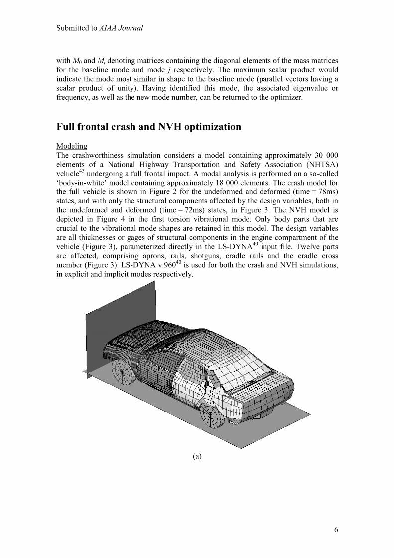
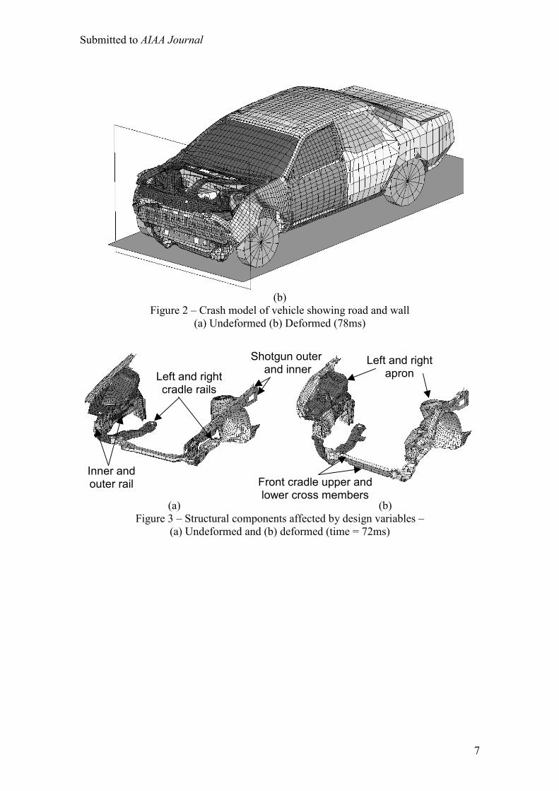
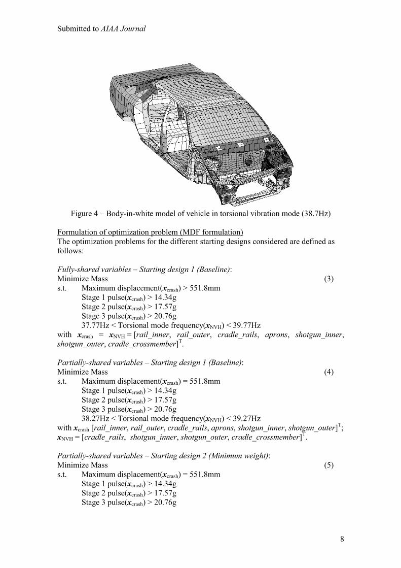
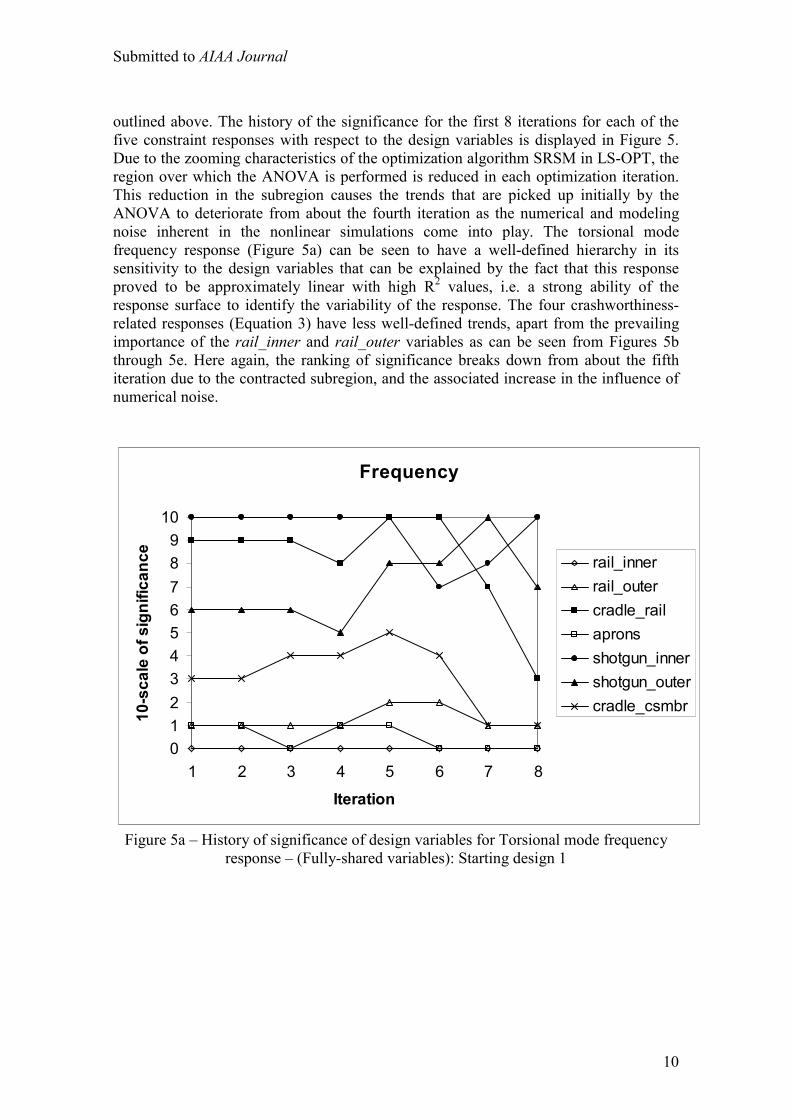
with M0 and Mj denoting matrices containing the diagonal elements of the mass matrices for the baseline mode and mode j respectively. The maximum scalar product would indicate the mode most similar in shape to the baseline mode (parallel vectors having a scalar product of unity). Having identified this mode, the associated eigenvalue or frequency, as well as the new mode number, can be returned to the optimizer. Full frontal crash and NVH optimization Modeling The crashworthiness simulation considers a model containing approximately 30 000 elements of a National Highway Transportation and Safety Association (NHTSA) vehicle43 undergoing a full frontal impact. A modal analysis is performed on a so-called ‘body-in-white’ model containing approximately 18 000 elements. The crash model for the full vehicle is shown in Figure 2 for the undeformed and deformed (time = 78ms) states, and with only the structural components affected by the design variables, both in the undeformed and deformed (time = 72ms) states, in Figure 3. The NVH model is depicted in Figure 4 in the first torsion vibrational mode. Only body parts that are crucial to the vibrational mode shapes are retained in this model. The design variables are all thicknesses or gages of structural components in the engine compartment of the vehicle (Figure 3), parameterized directly in the LS-DYNA40 input file. Twelve parts are affected, comprising aprons, rails, shotguns, cradle rails and the cradle cross member (Figure 3). LS-DYNA v.96040 is used for both the crash and NVH simulations, in explicit and implicit modes respectively.
(a)
Submitted to AIAA Journal
7
(b)
Figure 2 – Crash model of vehicle showing road and wall (a) Undeformed (b) Deformed (78ms)
(a)
(b)
Figure 3 – Structural components affected by design variables – (a) Undeformed and (b) deformed (time = 72ms)
Left and right apron
Inner and outer rail Front cradle upper and
lower cross members
Left and right cradle rails
Shotgun outer and inner
Submitted to AIAA Journal
8
Figure 4 – Body-in-white model of vehicle in torsional vibration mode (38.7Hz)
Formulation of optimization problem (MDF formulation) The optimization problems for the different starting designs considered are defined as follows: Fully-shared variables – Starting design 1 (Baseline): Minimize Mass (3) s.t. Maximum displacement(xcrash) > 551.8mm
Stage 1 pulse(xcrash) > 14.34g Stage 2 pulse(xcrash) > 17.57g Stage 3 pulse(xcrash) > 20.76g 37.77Hz < Torsional mode frequency(xNVH) < 39.77Hz
with xcrash = xNVH = [rail_inner, rail_outer, cradle_rails, aprons, shotgun_inner, shotgun_outer, cradle_crossmember]T. Partially-shared variables – Starting design 1 (Baseline): Minimize Mass (4) s.t. Maximum displacement(xcrash) = 551.8mm
Stage 1 pulse(xcrash) > 14.34g Stage 2 pulse(xcrash) > 17.57g Stage 3 pulse(xcrash) > 20.76g 38.27Hz < Torsional mode frequency(xNVH) < 39.27Hz
with xcrash [rail_inner, rail_outer, cradle_rails, aprons, shotgun_inner, shotgun_outer]T; xNVH = [cradle_rails, shotgun_inner, shotgun_outer, cradle_crossmember]T. Partially-shared variables – Starting design 2 (Minimum weight): Minimize Mass (5) s.t. Maximum displacement(xcrash) = 551.8mm
Stage 1 pulse(xcrash) > 14.34g Stage 2 pulse(xcrash) > 17.57g Stage 3 pulse(xcrash) > 20.76g

Submitted to AIAA Journal
9
38.27Hz < Torsional mode frequency(xNVH) < 39.27Hz with xcrash [rail_inner, rail_outer, cradle_rails, aprons]T; xNVH = [cradle_rails, shotgun_inner, shotgun_outer, cradle_crossmember]T.
Partially-shared variables – Starting design 3 (Maximum weight): Minimize Mass (6) s.t. Maximum displacement(xcrash) = 551.8mm
Stage 1 pulse(xcrash) > 14.34g Stage 2 pulse(xcrash) > 17.57g Stage 3 pulse(xcrash) > 20.76g 38.27Hz < Torsional mode frequency(xNVH) < 39.27Hz
with xcrash [rail_inner, rail_outer, cradle_rails, aprons, shotgun_inner, shotgun_outer, cradle crossmember]T; xNVH = [cradle_rails, shotgun_inner, shotgun_outer, cradle_crossmember]T. The different variables sets in Equations (4-6) were obtained from ANOVA studies (see an example in the Results section below). The Mass objective in each case incorporates all the components defined in Figure 3. The allowable torsional mode frequency band is reduced to 1Hz for the partially-shared cases to provide an optimum design that is more similar to the baseline. The maximum displacement constraint is changed from an inequality constraint (Equation (3)) to an equality constraint in Equations (4-6) in an attempt to force the optimizer to better maintain the intrusion of the baseline design. This is especially required for the minimum weight starting design, where the intrusion is expected to initially be much higher than the baseline value. The three stage pulses are calculated from the SAE filtered (60Hz) acceleration40 and displacement of a left rear sill node in the following fashion:
Stage i pulse = –k ∫2
1
dd
dxa ; k = 0.5 for i = 1, 1.0 otherwise; (7)
with the limits (d1;d2) = (0;184); (184;334); (334;Max(displacement)) for i = 1,2,3 respectively, all displacement units in mm and the minus sign to convert acceleration to deceleration. The Stage 1 pulse is represented by a triangle with the peak value being the value used. In summary, the optimization problem has as its aim the minimization of the mass while maintaining the baseline characteristics of the model, i.e. not degrading its crush energy, intrusion or torsional frequency characteristics. A left rear sill node is used to monitor the displacement. The constraints are scaled using the target values to balance the violations of the different constraints. This scaling is only important in cases where multiple constraints are violated as in the current problem. Results and discussion Variable screening To perform variable screening, the results of the fully-shared MDF case starting with the baseline design as depicted in Figures 2 through 4 are subjected to an ANOVA as
Submitted to AIAA Journal
10
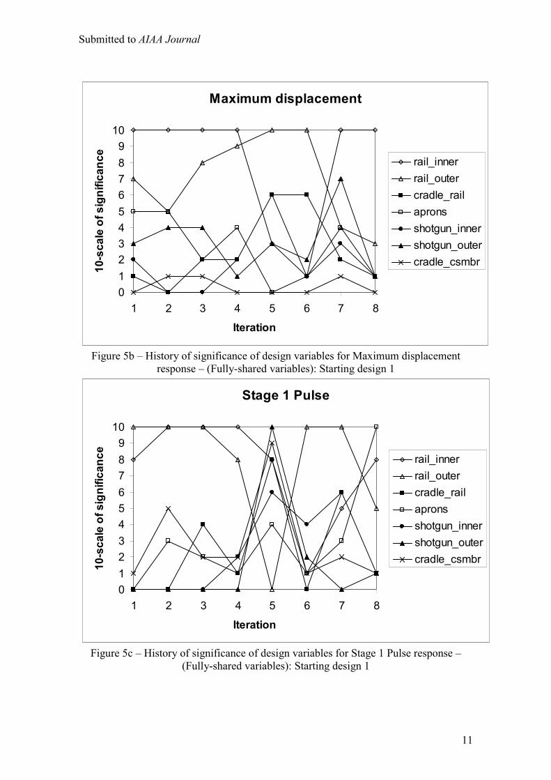
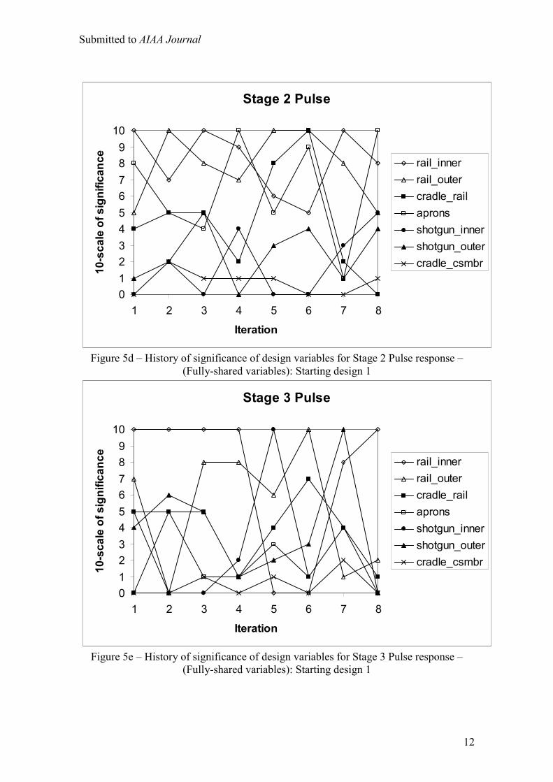
outlined above. The history of the significance for the first 8 iterations for each of the five constraint responses with respect to the design variables is displayed in Figure 5. Due to the zooming characteristics of the optimization algorithm SRSM in LS-OPT, the region over which the ANOVA is performed is reduced in each optimization iteration. This reduction in the subregion causes the trends that are picked up initially by the ANOVA to deteriorate from about the fourth iteration as the numerical and modeling noise inherent in the nonlinear simulations come into play. The torsional mode frequency response (Figure 5a) can be seen to have a well-defined hierarchy in its sensitivity to the design variables that can be explained by the fact that this response proved to be approximately linear with high R2 values, i.e. a strong ability of the response surface to identify the variability of the response. The four crashworthiness-related responses (Equation 3) have less well-defined trends, apart from the prevailing importance of the rail_inner and rail_outer variables as can be seen from Figures 5b through 5e. Here again, the ranking of significance breaks down from about the fifth iteration due to the contracted subregion, and the associated increase in the influence of numerical noise.
Frequency
0123456789
10
1 2 3 4 5 6 7 8
Iteration
10-s
cale
of s
igni
fican
ce rail_innerrail_outercradle_railapronsshotgun_innershotgun_outercradle_csmbr
Figure 5a – History of significance of design variables for Torsional mode frequency
response – (Fully-shared variables): Starting design 1
Submitted to AIAA Journal
11
Maximum displacement
0123456789
10
1 2 3 4 5 6 7 8
Iteration
10-s
cale
of s
igni
fican
ce rail_innerrail_outercradle_railapronsshotgun_innershotgun_outercradle_csmbr
Figure 5b – History of significance of design variables for Maximum displacement
response – (Fully-shared variables): Starting design 1
Stage 1 Pulse
0123456789
10
1 2 3 4 5 6 7 8
Iteration
10-s
cale
of s
igni
fican
ce rail_innerrail_outercradle_railapronsshotgun_innershotgun_outercradle_csmbr
Figure 5c – History of significance of design variables for Stage 1 Pulse response –
(Fully-shared variables): Starting design 1
Submitted to AIAA Journal
12
Stage 2 Pulse
0123456789
10
1 2 3 4 5 6 7 8
Iteration
10-s
cale
of s
igni
fican
ce rail_innerrail_outercradle_railapronsshotgun_innershotgun_outercradle_csmbr
Figure 5d – History of significance of design variables for Stage 2 Pulse response –
(Fully-shared variables): Starting design 1
Stage 3 Pulse
0123456789
10
1 2 3 4 5 6 7 8
Iteration
10-s
cale
of s
igni
fican
ce rail_innerrail_outercradle_railapronsshotgun_innershotgun_outercradle_csmbr
Figure 5e – History of significance of design variables for Stage 3 Pulse response –
(Fully-shared variables): Starting design 1
Submitted to AIAA Journal
13
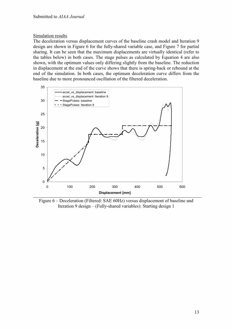
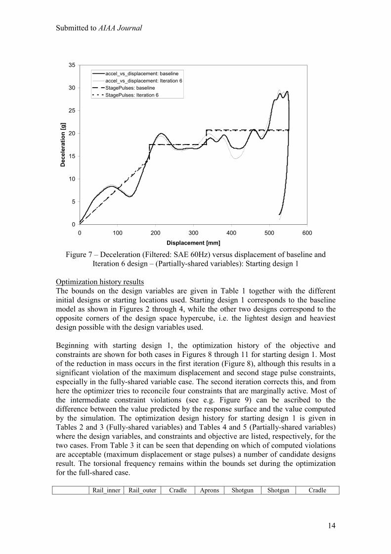
Simulation results The deceleration versus displacement curves of the baseline crash model and Iteration 9 design are shown in Figure 6 for the fully-shared variable case, and Figure 7 for partial sharing. It can be seen that the maximum displacements are virtually identical (refer to the tables below) in both cases. The stage pulses as calculated by Equation 4 are also shown, with the optimum values only differing slightly from the baseline. The reduction in displacement at the end of the curve shows that there is spring-back or rebound at the end of the simulation. In both cases, the optimum deceleration curve differs from the baseline due to more pronounced oscillation of the filtered deceleration.
0
5
10
15
20
25
30
35
0 100 200 300 400 500 600
Displacement [mm]
Dec
eler
atio
n [g
]
accel_vs_displacement: baselineaccel_vs_displacement: Iteration 9StagePulses: baselineStagePulses: Iteration 9
Figure 6 – Deceleration (Filtered: SAE 60Hz) versus displacement of baseline and
Iteration 9 design – (Fully-shared variables): Starting design 1
Submitted to AIAA Journal
14
0
5
10
15
20
25
30
35
0 100 200 300 400 500 600
Displacement [mm]
Dec
eler
atio
n [g
]
accel_vs_displacement: baselineaccel_vs_displacement: Iteration 6StagePulses: baselineStagePulses: Iteration 6
Figure 7 – Deceleration (Filtered: SAE 60Hz) versus displacement of baseline and
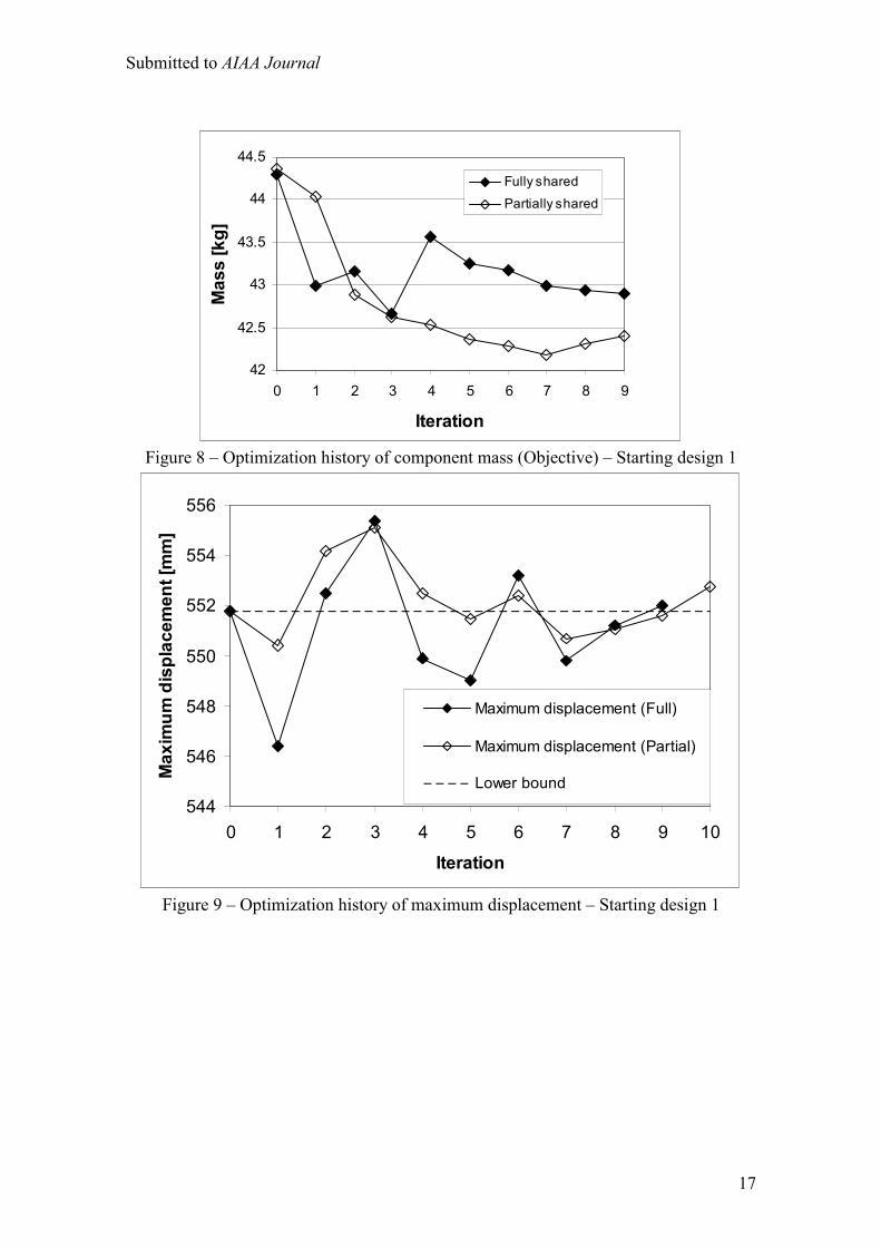
Iteration 6 design – (Partially-shared variables): Starting design 1 Optimization history results The bounds on the design variables are given in Table 1 together with the different initial designs or starting locations used. Starting design 1 corresponds to the baseline model as shown in Figures 2 through 4, while the other two designs correspond to the opposite corners of the design space hypercube, i.e. the lightest design and heaviest design possible with the design variables used. Beginning with starting design 1, the optimization history of the objective and constraints are shown for both cases in Figures 8 through 11 for starting design 1. Most of the reduction in mass occurs in the first iteration (Figure 8), although this results in a significant violation of the maximum displacement and second stage pulse constraints, especially in the fully-shared variable case. The second iteration corrects this, and from here the optimizer tries to reconcile four constraints that are marginally active. Most of the intermediate constraint violations (see e.g. Figure 9) can be ascribed to the difference between the value predicted by the response surface and the value computed by the simulation. The optimization design history for starting design 1 is given in Tables 2 and 3 (Fully-shared variables) and Tables 4 and 5 (Partially-shared variables) where the design variables, and constraints and objective are listed, respectively, for the two cases. From Table 3 it can be seen that depending on which of computed violations are acceptable (maximum displacement or stage pulses) a number of candidate designs result. The torsional frequency remains within the bounds set during the optimization for the full-shared case.
Rail_inner Rail_outer Cradle Aprons Shotgun Shotgun Cradle
Submitted to AIAA Journal
15
[mm] [mm] rail [mm] [mm] inner [mm] outer [mm]
cross member [mm]
Lower bound 1 1 1 1 1 1 1
Upper bound 3 3 2.5 2.5 3 3 2.5
Starting design 1
(Baseline) 2 1.5 1.93 1.3 1.3 1.3 1.930
Starting design 2
(Minimum weight)
1 1 1 1 1 1 1
Starting design 3
(Maximum weight)
3 3 2.5 2.5 3 3 2.5
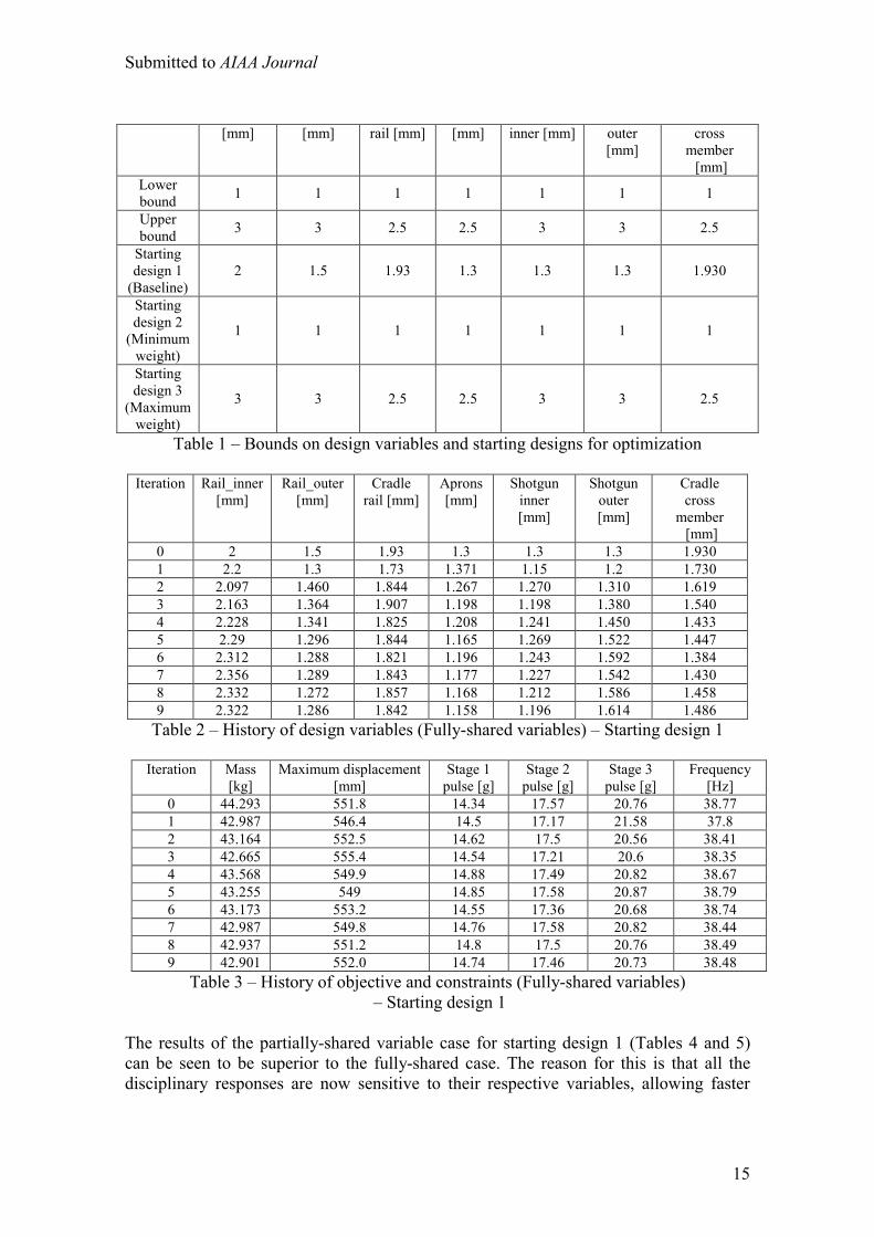
Table 1 – Bounds on design variables and starting designs for optimization
Iteration Rail_inner [mm]
Rail_outer [mm]
Cradle rail [mm]
Aprons [mm]
Shotgun inner [mm]
Shotgun outer [mm]
Cradle cross
member [mm]
0 2 1.5 1.93 1.3 1.3 1.3 1.930 1 2.2 1.3 1.73 1.371 1.15 1.2 1.730 2 2.097 1.460 1.844 1.267 1.270 1.310 1.619 3 2.163 1.364 1.907 1.198 1.198 1.380 1.540 4 2.228 1.341 1.825 1.208 1.241 1.450 1.433 5 2.29 1.296 1.844 1.165 1.269 1.522 1.447 6 2.312 1.288 1.821 1.196 1.243 1.592 1.384 7 2.356 1.289 1.843 1.177 1.227 1.542 1.430 8 2.332 1.272 1.857 1.168 1.212 1.586 1.458 9 2.322 1.286 1.842 1.158 1.196 1.614 1.486
Table 2 – History of design variables (Fully-shared variables) – Starting design 1
Iteration Mass [kg]
Maximum displacement [mm]
Stage 1 pulse [g]
Stage 2 pulse [g]
Stage 3 pulse [g]
Frequency [Hz]
0 44.293 551.8 14.34 17.57 20.76 38.77 1 42.987 546.4 14.5 17.17 21.58 37.8 2 43.164 552.5 14.62 17.5 20.56 38.41 3 42.665 555.4 14.54 17.21 20.6 38.35 4 43.568 549.9 14.88 17.49 20.82 38.67 5 43.255 549 14.85 17.58 20.87 38.79 6 43.173 553.2 14.55 17.36 20.68 38.74 7 42.987 549.8 14.76 17.58 20.82 38.44 8 42.937 551.2 14.8 17.5 20.76 38.49 9 42.901 552.0 14.74 17.46 20.73 38.48
Table 3 – History of objective and constraints (Fully-shared variables) – Starting design 1
The results of the partially-shared variable case for starting design 1 (Tables 4 and 5) can be seen to be superior to the fully-shared case. The reason for this is that all the disciplinary responses are now sensitive to their respective variables, allowing faster
Submitted to AIAA Journal
16
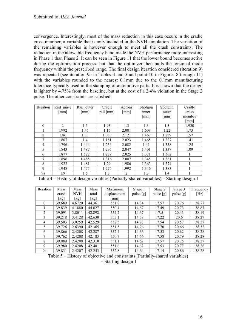
convergence. Interestingly, most of the mass reduction in this case occurs in the cradle cross member, a variable that is only included in the NVH simulation. The variation of the remaining variables is however enough to meet all the crash constraints. The reduction in the allowable frequency band made the NVH performance more interesting in Phase 1 than Phase 2. It can be seen in Figure 11 that the lower bound becomes active during the optimization process, but that the optimizer then pulls the torsional mode frequency within the prescribed range. The final design iteration considered (iteration 9) was repeated (see iteration 9a in Tables 4 and 5 and point 10 in Figures 8 through 11) with the variables rounded to the nearest 0.1mm due to the 0.1mm manufacturing tolerance typically used in the stamping of automotive parts. It is shown that the design is lighter by 4.75% from the baseline, but at the cost of a 2.4% violation in the Stage 2 pulse. The other constraints are satisfied.
Iteration Rail_inner [mm]
Rail_outer [mm]
Cradle rail [mm]
Aprons [mm]
Shotgun inner [mm]
Shotgun outer [mm]
Cradle cross
member [mm]
0 2 1.5 1.93 1.3 1.3 1.3 1.930 1 1.992 1.45 1.15 2.001 1.608 1.22 1.73 2 1.86 1.33 1.083 2.121 1.467 1.259 1.57 3 1.807 1.4 1.181 2.023 1.465 1.327 1.41 4 1.796 1.444 1.236 2.082 1.41 1.338 1.25 5 1.843 1.487 1.295 2.047 1.401 1.337 1.09 6 1.877 1.522 1.279 2.025 1.371 1.362 1 7 1.896 1.485 1.316 2.007 1.345 1.361 1 8 1.922 1.481 1.29 1.986 1.363 1.374 1 9 1.948 1.475 1.275 1.992 1.346 1.383 1 9a 1.9 1.5 1.3 2 1.3 1.4 1
Table 4 – History of design variables (Partially-shared variables) – Starting design 1
Iteration Mass crash [kg]
Mass NVH [kg]
Mass total [kg]
Maximum displacement
[mm]
Stage 1 pulse [g]
Stage 2 pulse [g]
Stage 3 pulse [g]
Frequency [Hz]
0 39.689 4.6720 44.361 551.8 14.34 17.57 20.76 38.77 1 39.839 4.1880 44.027 550.4 14.67 17.49 20.73 38.87 2 39.091 3.8011 42.892 554.2 14.67 17.5 20.41 38.19 3 39.218 3.4128 42.630 555.1 14.58 17.22 20.6 38.27 4 39.503 3.0259 42.529 552.5 14.73 17.54 20.57 38.27 5 39.726 2.6390 42.365 551.5 14.76 17.70 20.66 38.32 6 39.866 2.4208 42.287 552.4 14.66 17.53 20.62 38.28 7 39.762 2.4208 42.183 550.7 14.66 17.58 20.79 38.28 8 39.889 2.4208 42.310 551.1 14.62 17.57 20.75 38.27 9 39.980 2.4208 42.401 551.6 14.62 17.53 20.77 38.26 9a 39.831 2.4207 42.253 552.8 14.64 17.14 20.86 38.28
Table 5 – History of objective and constraints (Partially-shared variables) – Starting design 1
Submitted to AIAA Journal
17
42
42.5
43
43.5
44
44.5
0 1 2 3 4 5 6 7 8 9
Iteration
Mas
s [k
g]
Fully sharedPartially shared
Figure 8 – Optimization history of component mass (Objective) – Starting design 1
544
546
548
550
552
554
556
0 1 2 3 4 5 6 7 8 9 10
Iteration
Max
imum
dis
plac
emen
t [m
m]
Maximum displacement (Full)
Maximum displacement (Partial)
Lower bound
Figure 9 – Optimization history of maximum displacement – Starting design 1

Submitted to AIAA Journal
18
14
15
16
17
18
19
20
21
22
0 1 2 3 4 5 6 7 8 9 10Iteration
Acc
eler
atio
n [g
]
Stage1Pulse (Full)Stage2Pulse (Full)Stage3Pulse (Full)Stage1Pulse (Partial)Stage2Pulse (Partial)Stage3Pulse (Partial)Lower bound: Stage 1Lower bound: Stage 2Lower bound: Stage 3
Figure 10 – Optimization history of Stage pulses – Starting design 1
37.5
38
38.5
39
39.5
40
0 1 2 3 4 5 6 7 8 9 10
Iteration
Freq
uenc
y [H
z]
Frequency (Full)
Frequency (Partial)
Upper bound (Full)
Lower bound (Full)
Upper bound (Partial)
Lower bound (Partial)
Figure 11 – Optimization history of torsional mode frequency – Starting design 1
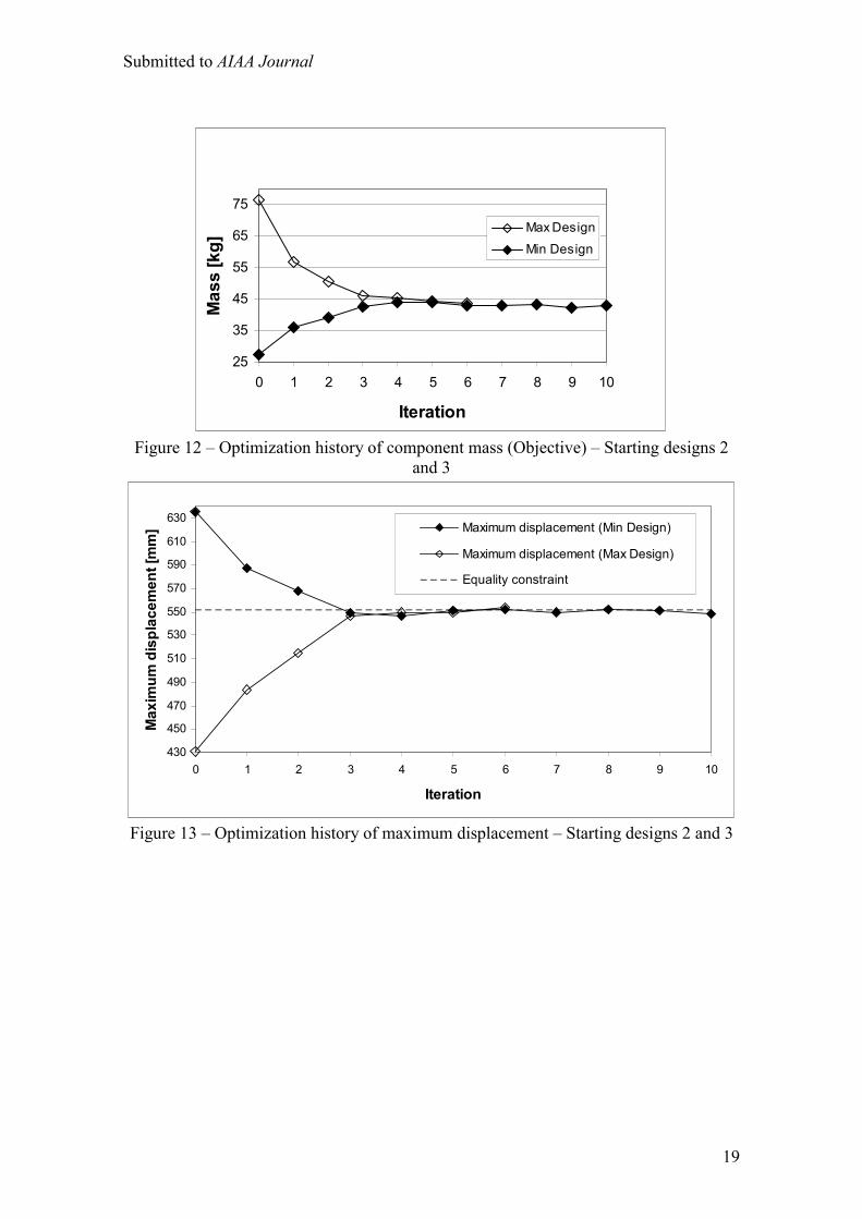
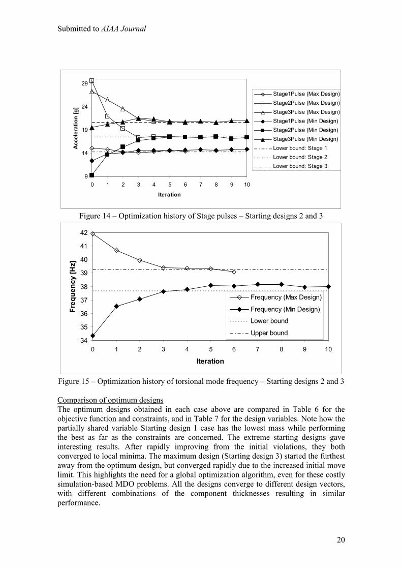
The results for the heaviest and lightest starting designs (2 and 3) are given in Figures 12 through 15. In both cases, an ANOVA was performed after one iteration of full sharing only in order to reduce the discipline-specific variables. The optimization was then restarted using the variable sets as defined in Equations (5) and (6). As expected, both designs converge to an intermediate mass in an attempt to satisfy all the constraints. The heaviest design history exhibits the largest mass change because of the significant increase in the thickness of the components over the baseline design.
Submitted to AIAA Journal
19
25
35
45
55
65
75
0 1 2 3 4 5 6 7 8 9 10
Iteration
Mas
s [k
g]Max DesignMin Design
Figure 12 – Optimization history of component mass (Objective) – Starting designs 2
and 3
430
450
470
490
510
530
550
570
590
610
630
0 1 2 3 4 5 6 7 8 9 10
Iteration
Max
imum
dis
plac
emen
t [m
m] Maximum displacement (Min Design)
Maximum displacement (Max Design)
Equality constraint
Figure 13 – Optimization history of maximum displacement – Starting designs 2 and 3
Submitted to AIAA Journal
20
9
14
19
24
29
0 1 2 3 4 5 6 7 8 9 10
Iteration
Acce
lera
tion
[g]
Stage1Pulse (Max Design)Stage2Pulse (Max Design)Stage3Pulse (Max Design)Stage1Pulse (Min Design)Stage2Pulse (Min Design)Stage3Pulse (Min Design)Lower bound: Stage 1Lower bound: Stage 2Lower bound: Stage 3
Figure 14 – Optimization history of Stage pulses – Starting designs 2 and 3
34
35
36
37
38
39
40
41
42
0 1 2 3 4 5 6 7 8 9 10
Iteration
Freq
uenc
y [H
z]
Frequency (Max Design)
Frequency (Min Design)
Lower bound
Upper bound
Figure 15 – Optimization history of torsional mode frequency – Starting designs 2 and 3 Comparison of optimum designs The optimum designs obtained in each case above are compared in Table 6 for the objective function and constraints, and in Table 7 for the design variables. Note how the partially shared variable Starting design 1 case has the lowest mass while performing the best as far as the constraints are concerned. The extreme starting designs gave interesting results. After rapidly improving from the initial violations, they both converged to local minima. The maximum design (Starting design 3) started the furthest away from the optimum design, but converged rapidly due to the increased initial move limit. This highlights the need for a global optimization algorithm, even for these costly simulation-based MDO problems. All the designs converge to different design vectors, with different combinations of the component thicknesses resulting in similar performance.
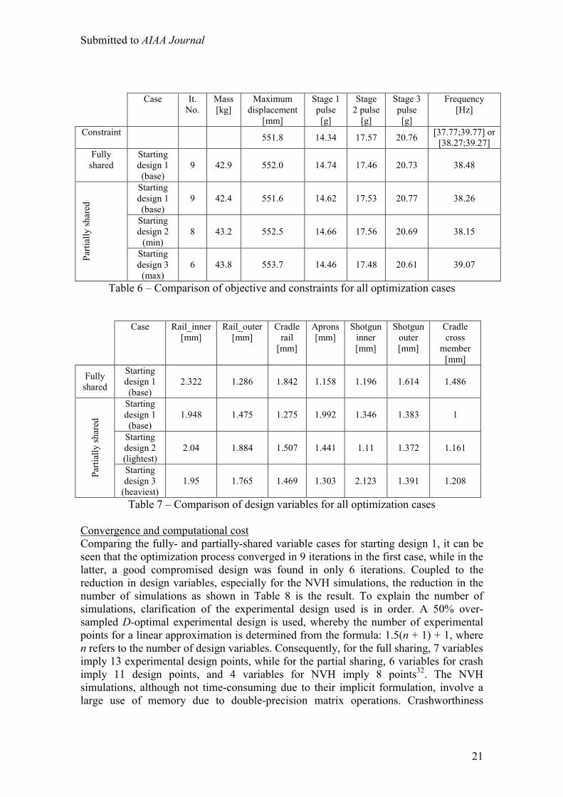
Submitted to AIAA Journal
21
Case It.
No. Mass [kg]
Maximum displacement
[mm]
Stage 1 pulse [g]
Stage 2 pulse
[g]
Stage 3 pulse [g]
Frequency [Hz]
Constraint 551.8 14.34 17.57 20.76 [37.77;39.77] or [38.27;39.27]
Fully shared
Starting design 1 (base)
9 42.9 552.0 14.74 17.46 20.73 38.48
Starting design 1 (base)
9 42.4 551.6 14.62 17.53 20.77 38.26
Starting design 2
(min) 8 43.2 552.5 14.66 17.56 20.69 38.15
Parti
ally
shar
ed
Starting design 3 (max)
6 43.8 553.7 14.46 17.48 20.61 39.07
Table 6 – Comparison of objective and constraints for all optimization cases
Case Rail_inner [mm]
Rail_outer [mm]
Cradle rail
[mm]
Aprons [mm]
Shotgun inner [mm]
Shotgun outer [mm]
Cradle cross
member [mm]
Fully shared
Starting design 1 (base)
2.322 1.286 1.842 1.158 1.196 1.614 1.486
Starting design 1 (base)
1.948 1.475 1.275 1.992 1.346 1.383 1
Starting design 2 (lightest)
2.04 1.884 1.507 1.441 1.11 1.372 1.161
Parti
ally
shar
ed
Starting design 3
(heaviest) 1.95 1.765 1.469 1.303 2.123 1.391 1.208
Table 7 – Comparison of design variables for all optimization cases Convergence and computational cost Comparing the fully- and partially-shared variable cases for starting design 1, it can be seen that the optimization process converged in 9 iterations in the first case, while in the latter, a good compromised design was found in only 6 iterations. Coupled to the reduction in design variables, especially for the NVH simulations, the reduction in the number of simulations as shown in Table 8 is the result. To explain the number of simulations, clarification of the experimental design used is in order. A 50% over-sampled D-optimal experimental design is used, whereby the number of experimental points for a linear approximation is determined from the formula: 1.5(n + 1) + 1, where n refers to the number of design variables. Consequently, for the full sharing, 7 variables imply 13 experimental design points, while for the partial sharing, 6 variables for crash imply 11 design points, and 4 variables for NVH imply 8 points32. The NVH simulations, although not time-consuming due to their implicit formulation, involve a large use of memory due to double-precision matrix operations. Crashworthiness
Submitted to AIAA Journal
22
simulations, on the other hand, require little memory because of single-precision vector operations, but are time-consuming due to their explicit nature. It is therefore preferable to assign as many processors as possible to the crashworthiness simulations, while limiting the number of simultaneous NVH simulations to the available computer memory to prevent swapping.
Table 8 – Number of simulations for Fully- and Partially-Shared Variable Cases (Starting design 1)
Conclusions The paper describes the multidisciplinary feasible optimization of a full vehicle model considering crashworthiness and NVH design criteria. A linear successive response surface approach is used to conduct the optimization. Using partially shared variables, a component mass reduction of almost 5% is achieved while maintaining or improving the design criteria of the baseline design. The optimization using partially shared variables converges more rapidly than when using fully shared variables, probably because of the elimination of uncertain variables using the ANOVA method based on the partial F-test. It is shown that the optimizer finds different optima when starting from different designs located in the extreme (minimum and maximum weight) corners of the design space. It is possible that a mode that is identified in the baseline design can become sufficiently obscured by the modes of a modified design. This happened in the case (maximum weight starting design) where the starting design was far away from the anticipated optimum design. A remedy could be to monitor intermediate designs to update the baseline vibration mode. Acknowledgements The authors would like to thank DaimlerChrysler for the use of their computing facilities for part of this study. They would like to acknowledge the support from the South African National Research Foundation, Grant no. GUN2046904, for the sabbatical of the first author at the Livermore Software Technology Corporation from the University of Pretoria, South Africa. The authors are also indebted to Suri Balasubramanyam of LSTC for assisting with the collaboration between LSTC and DaimlerChrysler. The computational resources used in this study included Compaq Alpha, IBM SP, and Hewlett Packard V-Class computers.
Case Number of crash simulations for ‘convergence’
Number of NVH simulations for ‘convergence’
Fully-shared variables 9 x 13 = 127 9 x 13 = 127 Partially-shared variables 6 x 11 = 66 6 x 8 = 48
Submitted to AIAA Journal
23
References 1. Etman LFP. Optimization of Multibody Systems using Approximation
Concepts. Ph.D. thesis, Technical University Eindhoven, The Netherlands 1997. 2. Etman LFP, Adriaens JMTA, van Slagmaat MTP, Schoofs AJG,
Crashworthiness Design Optimization using Multipoint Sequential Linear Programming. Structural Optimization 1996; 12:222-228.
3. Marklund P-O. Optimization of a Car Body Component Subjected to Impact. Linköping Studies in Science and Technology, Thesis No. 776, Department of Mechanical Engineering, Linköping University, Sweden 1999.
4. Marklund P-O., Nilsson L. Optimization of a Car Body Component Subjected to side Impact. Struct Multidisc Optim. 2001 21:383-392.
5. Akkerman A, Thyagarajan R, Stander N, Burger M, Kuhn R, Rajic H. Shape Optimization for Crashworthiness Design using Response Surfaces. Proceedings of the International Workshop on Multidisciplinary Design Optimization. Pretoria, South Africa, August 8-10, 2000, pp. 270-279.
6. Stander N. Optimization of Nonlinear Dynamic Problems using Successive Linear Approximations. AIAA Paper 2000-4798, 2000.
7. Schramm U, Thomas H. Crashworthiness design using structural optimization. AIAA Paper 98-4729, 1998.
8. Gu L. A comparison of polynomial based regression models in vehicle safety analysis. Paper DETC2001/DAC-21063. Proceedings of DETC’01 ASME 2001 Design Engineering Technical Engineering Conferences and the Computers and Information in Engineering Conference. Pittsburgh, PA. September 9-12, 2001.
9. Yang R-J, Wang N, Tho CH, Bobineau JP, Wang BP. Metamodeling development for vehicle frontal impact simulation. Paper DETC2001/DAC-21063. Proceedings of DETC’01 ASME 2001 Design Engineering Technical Engineering Conferences and the Computers and Information in Engineering Conference. Pittsburgh, PA. September 9-12, 2001.
10. Lewis K, Mistree F. The other side of multidisciplinary design optimization: accommodating a mutiobjective, uncertain and non-deterministic world. Engineering Optimization 1998 31:161-189.
11. Barthelemy J-F,M. (1983) Development of a multilevel optimization approach to the design of modern engineering systems. NASA/CR-172184-1983.
12. Haftka RT, Sobieszczanski-Sobieski J. Multidisciplinary aerospace design optimization: Survey of recent developments. AIAA Paper 96-0711, 1996.
13. Sobieszczanski-Sobieski J, Haftka RT. Multidisciplinary Aerospace Design Optimization: Survey of recent developments, Structural Optimization 1997; 14(1):1-23.
14. Sobieszczanski-Sobieski J, Kodiyalam S, Yang R-J. Optimization of car body under constraints of noise, vibration, and harshness (NVH), and crash. AIAA Paper 2000-1521, 2000.
15. Yang R-J, Gu L, Tho CH, Sobieszczanski-Sobieski J. Multidisciplinary design optimization of a full vehicle with high performance computing. AIAA Paper 2001-1273, 2001.
16. Schramm U. Multi-disciplinary optimization for NHV and crashworthiness. Proceedings of the First MIT Conference on Computational Fluid and Solid Mechanics. Bathe KJ, Ed., Boston, June 12-15, 2001. Elsevier Science Ltd., Oxford, pp.721:724.
Submitted to AIAA Journal
24
17. Alexandrov NM, Lewis RM. Analytical and computational properties of distributed approaches to MDO. AIAA Paper 2000-4718, 2000.
18. Alexandrov NM, Lewis RM. Algorithmic perspectives on problem formulations in MDO. AIAA Paper 2000-4719, 2000.
19. Michelena N, Papalambros PY. A network reliability approach to optimal decomposition of design problems. ASME Journal of Mechanical Design 1995; 117(3):433-440.
20. Renaud JE. A concurrent engineering approach for multidisciplinary design in a distributed computing environment. In Alexandrov NM, Hussaini MY. Eds. Multidisciplinary Design Optimization: State of the Art. 1997 SIAM.
21. Braun, R., Gage, P., Kroo, I., Sobieski, I., Implementation and performance issues in collaborative optimization, Sixth AIAA/USAF/NASA/ISSMO Symposium on Multidisciplinary Analysis and Optimization, Bellevue, Washington, AIAA Paper No. 96-4017, September 4-6, 1996.
22. Kroo I, Manning V. Collaborative optimization – status and directions. Eighth AIAA/USAF/NASA/ISSMO Symposium on Multidisciplinary Analysis and Optimization, Long Beach, CA, AIAA Paper No. 2000-4721, September 6-8, 2000.
23. Alexandrov NM, Lewis RM. Analytical and computational aspects of collaborative optimization. NASA/TM-2000-210104, 2000.
24. Batill SM, Stelmack MA, Stellar RS. Framework for multidisciplinary design based on response-surface approximations. Journal of Aircraft 1999; 36(1):287-297.
25. Sobieszczanski-Sobieski J, Agte J, Sandusky R Jr. Bi-level integrated system synthesis. AIAA Paper 98-4916, 1998.
26. Sobieszczanski-Sobieski J, Kodiyalam S. BLISS/S: a new method for two-level structural optimization. Struct Multidisc Optim. 2001 21:1-13.
27. Haftka RT, Gürdal A, Kamat MP. Elements of structural optimization. Kluwer Academic Publishers, Dordrect, 1990.
28. Cramer EJ, Dennis JE Jr, Frank PD, Lewis RM, Shubin GR. Problem formulations for multidisciplinary optimization. SIAM Journal of Optimization 1994; 40(4):754-776.
29. Zang TA, Green LL. Multidisciplinary Design Optimization techniques: Implications and opportunities for fluid dynamics research. AIAA Paper 99-3798, 1999.
30. Salas AO, Townsend JC. Framework Requirements for MDO Application Development, AIAA Paper 98-4740, 1998.
31. Craig KJ, Stander N. On the comparison of MDO formulations for automotive vehicle design using response surface methods, in preparation.
32. Stander N. LS-OPT User’s Manual Version 1, Livermore Software Technology Corporation, Livermore, CA, 1999.
33. Myers RH, Montgomery DC. Response Surface Methodology. Wiley: New York, 1995.
34. Snyman JA. The LFOPC leap-frog algorithm for constrained optimization. Computers and Mathematics with Applications 2000; 40:1085-1096.
35. Stander N, Craig KJ. On the robustness of the successive response surface method for simulation-based optimization. Submitted to Engineering Computations. July 2001.

Submitted to AIAA Journal
25
36. Stander, N. (2001) “The Successive Response Surface Method Applied to Sheet-Metal Forming”, Proceedings of the First MIT Conference on Computational Fluid and Solid Mechanics, Boston, June 12-14, 2001. Elsevier Science Ltd., Oxford.
37. Roux WJ, Stander N, Haftka RT. Response surface approximations for structural optimization. International Journal for Numerical Methods in Engineering 1998; 42:517-534.
38. Haftka RT, Gürdal Z. Elements of Structural Optimization. Kluwer: Dordrecht, 1990, p.257.
39. Stander N, Craig KJ. LS-OPT User’s Manual Version 2, Livermore Software Technology Corporation, Livermore, CA, 2001.
40. Livermore Software Technology Corporation. LS-DYNA manual version 960. Livermore, CA, 2001.
41. Bathe K-J, Wilson EL. Numerical Methods in Finite Element Analysis. Prentice-Hall: Inglewood Cliffs, New Jersey, 1976, chapter 10.
42. Hallquist JO. Private communication, 2001. 43. National Crash Analysis Center (NCAC). Public Finite Element Model Archive,
www.ncac.gwu.edu/archives/model/index.html 2001.