Multifield dynamics of Higgs inflation

The MIT Faculty has made this article openly available. Please share how this access benefits you. Your story matters.

Citation Greenwood, Ross N., David I. Kaiser, and Evangelos I. Sfakianakis.“Multifield Dynamics of Higgs Inflation.” Physical Review D 87.6(2013). © 2013 American Physical Society

As Published http://dx.doi.org/10.1103/PhysRevD.87.064021

Publisher American Physical Society

Version Final published version

Citable link http://hdl.handle.net/1721.1/79596

Terms of Use Article is made available in accordance with the publisher'spolicy and may be subject to US copyright law. Please refer to thepublisher's site for terms of use.

Multifield dynamics of Higgs inflation

Ross N. Greenwood,* David I. Kaiser,† and Evangelos I. Sfakianakis‡

Center for Theoretical Physics and Department of Physics, Massachusetts Institute of Technology,Cambridge, Massachusetts 02139, USA

(Received 25 January 2013; published 18 March 2013)

Higgs inflation is a simple and elegant model in which early-universe inflation is driven by the Higgs

sector of the Standard Model. The Higgs sector can support early-universe inflation if it has a large

nonminimal coupling to the Ricci spacetime curvature scalar. At energies relevant to such an inflationary

epoch, the Goldstone modes of the Higgs sector remain in the spectrum in renormalizable gauges, and

hence their effects should be included in the model’s dynamics. We analyze the multifield dynamics of

Higgs inflation and find that the multifield effects damp out rapidly after the onset of inflation, because of

the gauge symmetry among the scalar fields in this model. Predictions from Higgs inflation for observable

quantities, such as the spectral index of the power spectrum of primordial perturbations, therefore revert to

their familiar single-field form, in excellent agreement with recent measurements. The methods we

develop here may be applied to any multifield model with nonminimal couplings in which the N fields

obey an SOðN Þ symmetry in field space.

DOI: 10.1103/PhysRevD.87.064021 PACS numbers: 04.62.+v, 98.80.Cq

I. INTRODUCTION

The recent discovery at CERN of a scalar boson withHiggs-like properties [1] heightens the question of whetherthe Standard Model Higgs sector could have played inter-esting roles in the early universe, at energies well above theelectroweak symmetry-breaking scale. In particular, thesuggestive evidence for the Higgs boson raises the possi-bility to return to an original motivation for cosmologicalinflation, namely, to realize a phase of early-universe ac-celeration driven by a scalar field that is part of a well-motivated model from high-energy particle physics [2–4].

Higgs inflation [5] represents an elegant approach tobuilding a workable inflationary model based on realisticingredients from particle physics. In this model, a largenonminimal coupling of the Standard Model electroweakHiggs sector drives a phase of early-universe inflation.Such nonminimal couplings are generic: they arise asnecessary renormalization counterterms for scalar fieldsin curved spacetime [6–9]. Moreover, renormalization-group analyses indicate that for models with matter akinto the Standard Model, the nonminimal coupling, �, shouldgrow without bound with increasing energy scale [9].Previous analyses of Higgs inflation have found that �typically grows by at least an order of magnitude betweenthe electroweak symmetry-breaking scale and the infla-tionary scale [10–12].

The Standard Model Higgs sector includes four scalardegrees of freedom: the (real) Higgs scalar and threeGoldstone modes. In renormalizable gauges, all four scalarfields remain in the spectrum at high energies [12–16].

Thus the dynamics of Higgs inflation should be studiedas a multifield model with nonminimal couplings. Animportant feature of multifield models, which is absent insingle-field models, is that the fields’ trajectories can turnwithin field space as the system evolves. Such turns are anecessary (but not sufficient) condition for multifield mod-els to depart from the empirical predictions of simplesingle-field models [17–23].In this paper we analyze the background dynamics of

Higgs inflation, in which all four scalar fields of theStandard Model electroweak Higgs sector have nonmini-mal couplings. We find that multifield dynamics damp outquickly after the onset of inflation, before perturbations oncosmologically relevant length scales first cross the Hubbleradius. As regards observable quantities like the powerspectrum of primordial perturbations, the model thereforebehaves effectively as a single-field model. The multifielddynamics remain subdominant in Higgs inflation becauseof the particular symmetries of the Higgs sector. Closelyrelated models, which lack those symmetries, can produceconspicuous departures from the single-field case [23].We are principally interested here in the behavior of

classical background fields and long-wavelength perturba-tions, which behave essentially classically. Therefore webracket, for this analysis, the question of the unitarity ofHiggs inflation. Conflicting conclusions have been ad-vanced regarding whether the appropriate renormalizationcutoff scale for this model should be Mpl, Mpl=

ffiffiffi�

p, or

Mpl=�, where Mpl � ð8�GÞ�1=2 is the reduced Planck

mass [12,14,15,24,25]. Even if Higgs inflation might con-clusively be shown to violate unitarity, the techniquesdeveloped here for the analysis of multifield dynamicswill be relevant for related models that incorporate mul-tiple scalar fields with nonminimal couplings and symme-tries (such as gauge symmetries) that enforce specific

*rossng@mit.edu†dikaiser@mit.edu‡esfaki@mit.edu

PHYSICAL REVIEW D 87, 064021 (2013)

1550-7998=2013=87(6)=064021(13) 064021-1 � 2013 American Physical Society

relations among the couplings of the model. In particular,we expect that multifield effects in models with N scalarfields, in which the scalar fields obey an SOðN Þ symme-try, should damp out rapidly.

In Sec. II, we briefly introduce the multifield formalismand establish notation. We apply the formalism to Higgsinflation in Sec. III, and in Sec. IV we analyze the behaviorof the turn rate, which quantifies the rate at which thebackground trajectory of the system deviates from asingle-field case. We study how quickly the turn rate dampsto zero, both analytically and numerically, confirming thatfor Higgs inflation the turn rate becomes negligible withina few e-folds after the start of inflation. In Sec. V we turn toimplications for observable features of the primordialpower spectrum, confirming that multifield Higgs inflationreproduces the empirical predictions of previous single-field studies. Concluding remarks follow in Sec. VI.

II. MULTIFIELD DYNAMICS

Following the approach established in Ref. [23], weconsider models withN scalar fields in ð3þ 1Þ spacetimedimensions. We use Greek letters to label spacetime in-dices, �, � ¼ 0, 1, 2, 3; lowercase Latin letters to labelspatial indices, i, j ¼ 1, 2, 3; and uppercase Latin letters tolabel field-space indices, I, J ¼ 1; 2; . . . ;N . We also work

in terms of the reduced Planck mass,Mpl � ð8�GÞ�1=2. In

the Jordan frame, the action takes the form

SJordan ¼Z

d4xffiffiffiffiffiffiffi�~g

p �fð�IÞ ~R

� 1

2�IJ~g

��@��I@��

J � ~Vð�IÞ�: (1)

Here fð�IÞ is the nonminimal coupling function, and weuse tildes for quantities in the Jordan frame. We perform aconformal transformation to the Einstein frame by rescal-ing the spacetime metric tensor,

g��ðxÞ ¼ 2

M2pl

fð�IðxÞÞ~g��ðxÞ; (2)

so that the action in the Einstein frame becomes [26]

SEinstein ¼Z

d4xffiffiffiffiffiffiffi�g

p �M2pl

2R

� 1

2GIJg

��@��I@��

J � Vð�IÞ�: (3)

The potential in the Einstein frame, V, is related to theJordan-frame potential, ~V, as

Vð�IÞ ¼ M4pl

4f2ð�IÞ~Vð�IÞ; (4)

and the coefficients of the noncanonical kinetic terms are[26,27]

GIJð�KÞ ¼ M2pl

2fð�IÞ��IJ þ 3

fð�IÞ f;If;J�; (5)

where f;I ¼ @f=@�I. The nonminimal couplings induce a

field-space manifold in the Einstein frame that is notconformal to flat; GIJ serves as a metric on the curvedmanifold [26]. Therefore we adopt the covariant approachof Ref. [23], which respects the curvature of the field-spacemanifold.Varying Eq. (3) with respect to�I yields the equation of

motion,

h�I þ g���IJK@��

J@��K � GIKV;K ¼ 0; (6)

where h�I � g���I;�;� and �I

JKð�LÞ is the Christoffel

symbol for the field-space manifold, calculated in terms ofGIJ. We expand each scalar field to first order around itsclassical background value,

�Iðx�Þ ¼ ’IðtÞ þ ��Iðx�Þ; (7)

and also expand the scalar degrees of freedom of thespacetime metric to first order around a spatially flatFriedmann-Robertson-Walker metric [28–30]

ds2 ¼ �ð1þ 2AÞdt2 þ 2að@iBÞdxidtþ a2½ð1� 2c Þ�ij þ 2@i@jE�dxidxj; (8)

where aðtÞ is the scale factor. We further introduce acovariant derivative with respect to the field-space metricand a directional derivative along the background fields’trajectory, such that for any vector AI in the field-spacemanifold we have

DJAI ¼ @JA

I þ �IJKA

K;

DtAI � _’JDJA

I ¼ _AI þ �IJKA

J _’K;(9)

where overdots denote derivatives with respect to cosmictime, t.To background order, Eq. (6) becomes

Dt _’I þ 3H _’I þ GIKV;K ¼ 0; (10)

where all quantities involving GIJð�KÞ, Vð�IÞ, and theirderivatives are evaluated at background order in the fields:GIJ ! GIJð’KÞ and V ! Vð’IÞ. Following [17] we dis-tinguish between adiabatic and entropic directions in fieldspace by introducing a unit vector

�I � _’I

_�; (11)

where

_� � j _’Ij ¼ffiffiffiffiffiffiffiffiffiffiffiffiffiffiffiffiffiffiffiGIJ _’I _’J

q: (12)

The operator

sIJ � GIJ � �I�J (13)

GREENWOOD, KAISER, AND SFAKIANAKIS PHYSICAL REVIEW D 87, 064021 (2013)

064021-2

projects onto the subspace orthogonal to �I. Equation (10)then simplifies to

€�þ 3H _�þ V;� ¼ 0; (14)

where

V;� � �IV;I: (15)

The background dynamics likewise take the simple form

H2 ¼ 1

3M2pl

�1

2_�2 þ V

�; _H ¼ � 1

2M2pl

_�2; (16)

where H � _a=a is the Hubble parameter.We may also separate the perturbations into adiabatic

and entropic directions. Working to first order in perturba-tions, we introduce the gauge-invariant Mukhanov-Sasakivariables [28–31]

QI � ��I þ _’I

Hc (17)

and the projections

Q� � �IQI; �sI � sIJQ

J: (18)

The gauge-invariant curvature perturbation may be definedas Rc � c � ½H=ð�þ pÞ��q, where the perturbedenergy-momentum flux is given by T0

i ¼ @i�q [29,30].We then find that Rc is proportional to Q� [23]:

Rc ¼ H

_�Q�: (19)

Expanding Eq. (6) to first order and using the projections ofEq. (18), the perturbations Q� and �sI obey [23]

€Q� þ 3H _Q� þ�k2

a2þM�� �!2 � 1

M2pla

3

d

dt

�a3 _�2

H

��Q�

¼ 2d

dtð!J�s

JÞ � 2

�V;�

_�þ _H

H

�ð!J�s

JÞ (20)

and

D2t �s

I þ ½3H�IJ þ 2�I!J�Dt�s

I

þ�k2

a2�I

J þMIJ � 2�I

�M�J þ €�

_�!J

���sJ

¼ �2!I

�_Q� þ _H

HQ� � €�

_�Q�

�; (21)

where the mass-squared matrix is

MIJ � GIKðDJDKVÞ �RI

LMJ _’L _’M;

M�J � �IMIJ; M�� � �I�

JMIJ:

(22)

The turn rate [22,23] is given by

!I � Dt�I ¼ � 1

_�V;Ks

IK; (23)

and! � j!Ij. Equations (20) and (21) decouple if the turnrate vanishes, !I ¼ 0. In that case, Q� evolves just as in

the single-field case [22,23,28–30]. Given Eq. (19), thatmeans that the power spectrum of primordial perturbations,PR, would also evolve as in single-field models. Thus anecessary (but not sufficient) condition for multifieldmodels of this form to deviate from the empirical predic-tions of simple single-field models is for the turn rate to benonnegligible for some duration of the fields’ evolution,!I � 0.

III. APPLICATION TO HIGGS INFLATION

The matter contribution to Higgs inflation [5] consists ofthe Standard Model electroweak Higgs sector, which maybe written as a doublet of complex scalar fields,

h ¼ hþ

h0

!: (24)

The complex fields hþ and h0 may be further decomposedinto (real) scalar degrees of freedom,

hþ ¼ 1ffiffiffi2

p ð1 þ i2Þ; h0 ¼ 1ffiffiffi2

p ð�þ i3Þ; (25)

where � is the Higgs scalar and a (with a ¼ 1, 2, 3) arethe Goldstone modes. In the Jordan frame, the potential~Vð�IÞ depends only on the combination

hyh ¼ 1

2½�2 þ �2�; (26)

where � ¼ ð1; 2; 3Þ is a three-vector of the Goldstonefields. In particular, the symmetry-breaking potential maybe written

~Vð�IÞ ¼

4ð�2 þ �2 � v2Þ2; (27)

in terms of the vacuum expectation value, v. For theStandard Model, v ¼ 246 GeV � Mpl. For Higgs infla-

tion, the nonminimal coupling function is given by

fð�IÞ ¼ M20

2þ �hyh ¼ 1

2½M2

0 þ �ð�2 þ �2Þ�; (28)

where M20 � M2

pl � �v2 and � > 0 is the dimensionless

nonminimal coupling constant. In Higgs inflation, wetake ��Oð104Þ [5], and therefore we may safely setM2

0 ¼ M2pl. In the Einstein frame, the potential gets

stretched by the nonminimal coupling function fð�IÞ ac-cording to Eq. (4). Given Eqs. (27) and (28), this yields

Vð�IÞ ¼ M4plð�2 þ �2 � v2Þ2

4½M2pl þ �ð�2 þ �2Þ�2 : (29)

The model is thus symmetric under rotations among� and

a that preserve the magnitudeffiffiffiffiffiffiffiffiffiffiffiffiffiffiffiffiffiffi�2 þ �2

p. When written

in the ‘‘Cartesian’’ field-space basis of Eq. (25), in otherwords, the SUð2Þ electroweak gauge symmetry manifestsas an SOð4Þ spherical symmetry in field space.

MULTIFIELD DYNAMICS OF HIGGS INFLATION PHYSICAL REVIEW D 87, 064021 (2013)

064021-3

For any model with N real-valued scalar fields thatrespects an SOðN Þ symmetry, the background dynamicsdepend on just three initial conditions: the initial magni-tude and initial velocity along the radial direction in fieldspace, and the initial velocity perpendicular to the radialdirection. Without loss of generality, therefore, we mayanalyze the background dynamics of Higgs inflation interms of just two real-valued scalar fields, � and , andwe may set ð0Þ ¼ 0, specifying only initial values for

�ð0Þ, _�ð0Þ, and _ð0Þ. This reduction in the effective num-ber of degrees of freedom stems entirely from the gaugesymmetry of the Standard Model electroweak sector. Theremaining dependence on _, meanwhile, distinguishes thebackground dynamics from a genuinely single-field model,in which one neglects the Goldstone fields altogether. Forthe remainder of this paper, we exploit the gauge symmetryto consider only a single Goldstone mode, � ! , reduc-ing the problem to that of a two-field model. Then fð�IÞand Vð�IÞ depend on the background fields only in thecombination

r �ffiffiffiffiffiffiffiffiffiffiffiffiffiffiffiffiffiffi�2 þ 2

q: (30)

Previous analyses [5,27,32–34] which consideredsingle-field versions of this model (neglecting theGoldstone modes) found successful inflation for field val-ues ��2 � M2

pl. We confirm this below for the multifield

case including the Goldstone modes. The reason is easy tosee from Eq. (29). In the limit �ð�2 þ 2Þ ¼ �r2 � M2

pl,

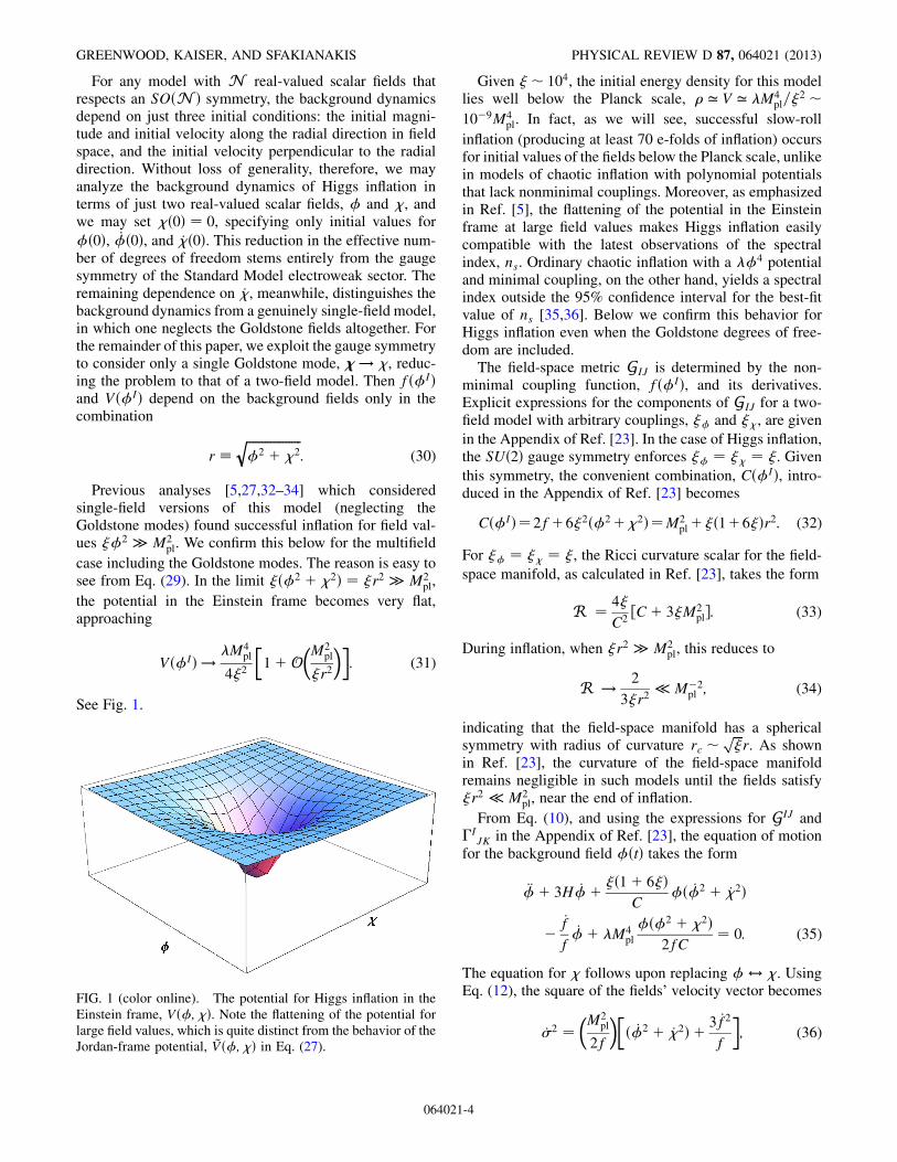
the potential in the Einstein frame becomes very flat,approaching

Vð�IÞ ! M4pl

4�2

�1þO

�M2pl

�r2

��: (31)

See Fig. 1.

Given �� 104, the initial energy density for this modellies well below the Planck scale, � ’ V ’ M4

pl=�2 �

10�9M4pl. In fact, as we will see, successful slow-roll

inflation (producing at least 70 e-folds of inflation) occursfor initial values of the fields below the Planck scale, unlikein models of chaotic inflation with polynomial potentialsthat lack nonminimal couplings. Moreover, as emphasizedin Ref. [5], the flattening of the potential in the Einsteinframe at large field values makes Higgs inflation easilycompatible with the latest observations of the spectralindex, ns. Ordinary chaotic inflation with a �4 potentialand minimal coupling, on the other hand, yields a spectralindex outside the 95% confidence interval for the best-fitvalue of ns [35,36]. Below we confirm this behavior forHiggs inflation even when the Goldstone degrees of free-dom are included.The field-space metric GIJ is determined by the non-

minimal coupling function, fð�IÞ, and its derivatives.Explicit expressions for the components of GIJ for a two-field model with arbitrary couplings, �� and �, are given

in the Appendix of Ref. [23]. In the case of Higgs inflation,the SUð2Þ gauge symmetry enforces �� ¼ � ¼ �. Given

this symmetry, the convenient combination, Cð�IÞ, intro-duced in the Appendix of Ref. [23] becomes

Cð�IÞ¼2fþ6�2ð�2þ2Þ¼M2plþ�ð1þ6�Þr2: (32)

For �� ¼ � ¼ �, the Ricci curvature scalar for the field-

space manifold, as calculated in Ref. [23], takes the form

R ¼ 4�

C2½Cþ 3�M2

pl�: (33)

During inflation, when �r2 � M2pl, this reduces to

R ! 2

3�r2� M�2

pl ; (34)

indicating that the field-space manifold has a sphericalsymmetry with radius of curvature rc �

ffiffiffi�

pr. As shown

in Ref. [23], the curvature of the field-space manifoldremains negligible in such models until the fields satisfy�r2 � M2

pl, near the end of inflation.

From Eq. (10), and using the expressions for GIJ and�I

JK in the Appendix of Ref. [23], the equation of motionfor the background field �ðtÞ takes the form

€�þ 3H _�þ �ð1þ 6�ÞC

�ð _�2 þ _2Þ

�_f

f_�þ M4

pl

�ð�2 þ 2Þ2fC

¼ 0: (35)

The equation for follows upon replacing � $ . UsingEq. (12), the square of the fields’ velocity vector becomes

_�2 ¼�M2

pl

2f

��ð _�2 þ _2Þ þ 3 _f2

f

�; (36)

FIG. 1 (color online). The potential for Higgs inflation in theEinstein frame, Vð�;Þ. Note the flattening of the potential forlarge field values, which is quite distinct from the behavior of theJordan-frame potential, ~Vð�;Þ in Eq. (27).

GREENWOOD, KAISER, AND SFAKIANAKIS PHYSICAL REVIEW D 87, 064021 (2013)

064021-4

and the gradient of the potential in the direction �I

becomes

�IV;I ¼ V;� ¼ M6plð�2 þ 2Þ�ð2fÞ3

_f

_�: (37)

We may verify that multifield Higgs inflation exhibitsslow-roll behavior for typical choices of couplings andinitial conditions. First consider the single-field case, inwhich we set ¼ _ ¼ 0. Near the start of inflation (with��2 � M2

pl), the terms in Eq. (35) that stem from the

field’s noncanonical kinetic term take the form

�ð1þ 6�ÞC

� _�2 �_f

f_� ! �

_�2

�: (38)

The usual slow-roll requirement for single-field models,

j _�j � jH�j, ensures that the terms in Eq. (38) remain

much less than the 3H _� term in Eq. (35). Neglecting €�,the single-field, slow-roll limit of Eq. (35) becomes

3H _� ’ � M4pl

6�3�; (39)

or, upon using H2 ’ V=ð3M2plÞ,

_� ’ �ffiffiffiffi

pM3

pl

3ffiffiffi3

p�2�

: (40)

Setting � ¼ 104 and fixing the initial field velocity byEq. (40) requires �ð0Þ � 0:1Mpl to yield N � 70 e-folds

of inflation in the single-field case.A much broader range of initial conditions yields

N � 70 e-folds in the two-field case. From Eq. (16) wesee that inflation (with €a > 0) requires _�2 � V. Given theSOðN Þ symmetry of the model, we may set ð0Þ ¼ 0without loss of generality, and parametrize the fields’initial velocities as

_�ð0Þ ¼ffiffiffiffi

pM3

pl

3ffiffiffi3

p�2�ð0Þ x; _ð0Þ ¼

ffiffiffiffi

pM3

pl

3ffiffiffi3

p�2�ð0Þ y (41)

in terms of dimensionless constants x and y. (The single-field case corresponds to x ¼ �1, y ¼ 0.) Near the start ofinflation, when �r2 ¼ ��2 � M2

pl, Eq. (36) becomes

_�2jð0Þ¼0 !�M4

pl

4�2

�� M2pl

��2ð0Þ�2 4

27�½ð1þ 6�Þx2 þ y2�:

(42)

The first term in parentheses is just the value of the poten-tial, V, near the start of inflation, as given in Eq. (31). Thesecond term in parentheses is small near the beginning of

inflation, given �r2 � M2pl. Hence the initial values for

_�

and _, parametrized by the coefficients x and y, may besubstantially larger than in the single-field case while stillkeeping _�2 � V.

Figure 2 shows HðtÞ, �ðtÞ, and ðtÞ for a scenario in

which _�ð0Þ and _ð0Þ greatly exceed the single-field relationof Eq. (40): jxj ¼ 102 and jyj ¼ 106. As is evident in thefigure, the large initial velocities cause the fields to oscillaterapidly. The extra kinetic energy makes the initial value ofHðtÞ larger than in the corresponding single-field case. Theincrease in H, in turn, causes the fields’ velocities to damp

out even more quickly, due to the 3H _� and 3H _ Hubble-drag terms in each field’s equation of motion. Thus thesystem rapidly settles into a slow-roll regime that continuesfor 70 e-folds. As shown in Fig. 3, we may achieve N � 70e-folds with even smaller initial field values by making theinitial field velocities correspondingly larger.

IV. TURN RATE

The components of the turn rate, !I in Eq. (23), takethe form

!� ¼ �M4pl

_�

r2

2f

��

C�M2

pl

4f2

_�

_�2ð� _�þ _Þ

�: (43)

The other component, !, follows upon replacing � $ .The length of the turn-rate vector is given by

! ¼ j!Ij ¼ffiffiffiffiffiffiffiffiffiffiffiffiffiffiffiffiffiffiffiGIJ!

I!Jq

¼ 1

_�

ffiffiffiffiffiffiffiffiffiffiffiffiffiffiffiffiffiffiffiffiffiffiffisKMV;KV;M

q; (44)

where the final expression follows upon using the defini-tion of !I in Eq. (23) and the identity sKM ¼ sKAs

MA,which follows from Eq. (13). We find

FIG. 2 (color online). The evolution of HðtÞ (black dashedline) and the fields �ðtÞ (red solid line) and ðtÞ (blue dottedline). The fields are measured in units of Mpl and we use the

dimensionless time variable � ¼ ffiffiffiffi

pMplt. We have plotted 103H

so that its scale is commensurate with the magnitude of thefields. The Hubble parameter begins large, Hð0Þ ¼ 8:1� 10�4,but quickly falls by a factor of 30 as it settles to its slow-rollvalue of H ¼ 2:8� 10�5. Inflation proceeds for �� ¼ 2:5�106 to yield N ¼ 70:7 e-folds of inflation. The solutions shownhere correspond to � ¼ 104, �ð0Þ ¼ 0:1, ð0Þ ¼ 0, _�ð0Þ ¼�2� 10�6, and _ð0Þ ¼ 2� 10�2. For the same value of�ð0Þ, Eq. (40) corresponds to _�ð0Þ ¼ �2� 10�8 for thesingle-field case.

MULTIFIELD DYNAMICS OF HIGGS INFLATION PHYSICAL REVIEW D 87, 064021 (2013)

064021-5

_�2!2¼ sKMV;KV;M¼ 2M10pl

ð2fÞ5Cr6½C��2r2��ðV;�Þ2: (45)

The evolution of the turn rate for typical initial conditionsis shown in Fig. 4.

In order to analyze the evolution of the backgroundfields, it is easier to move from Cartesian to polar coor-dinates, in which the angular velocity and turn ratehave more intuitive behavior. In addition to the radius,r2 ¼ �2 þ 2, we also define the angle

� � arctan

�

�

�: (46)

Single-field trajectories correspond to constant �ðtÞ. In thepolar coordinate system, the background dynamics ofEq. (16) may be written

H2 ¼ 1

12f

�_r2 þ r2 _�2 þ 3�2

fr2 _r2 þ M2

pl

2

r4

ðM2pl þ �r2Þ

�;

_H ¼ � 1

4f

�_r2 þ r2 _�2 þ 3�2

fr2 _r2

�: (47)

The equations of motion become

€rþ 3H _r� r _�2 þ �ð1þ 6�ÞC

rð _r2 þ r2 _�2Þ

� �

f_r2rþ M4

pl

r3

2fC¼ 0 (48)

and

€�þ�3H þ 2

_r

r

M2pl

ðM2pl þ �r2Þ

�_� ¼ 0: (49)

In this new basis the turn rate may be written compactlyas

!2 ¼ 2M8pl

2fC

�r4 _�

r2 _�2ðM2pl þ �r2Þ þ _r2C

�2: (50)

This expression vanishes in both the limits j _�j ! 0 andj _�j ! 1: if the angular velocity is either too large or toosmall, the fields’ evolution reverts to effectively single-field behavior (either purely radial motion or purely angu-lar motion). Of the two limits, however, only pure-radial

FIG. 3 (color online). Contour plots showing the number of e-folds of inflation as one varies the fields’ initial conditions, keeping� ¼ 104 fixed. In each panel, the vertical axis is _ð0Þ and the horizontal axis is _�ð0Þ. The panels correspond to �ð0Þ ¼ 10�1Mpl

(top left), 10�2Mpl (top right), 5� 10�3Mpl (bottom left), and 10�4Mpl (bottom right), and we again use dimensionless time� ¼ ffiffiffiffi

p

Mplt. In each panel, the line for N ¼ 70 e-folds is shown in bold. Note how large these initial velocities are compared to thesingle-field expectation of Eq. (40).

GREENWOOD, KAISER, AND SFAKIANAKIS PHYSICAL REVIEW D 87, 064021 (2013)

064021-6

motion is stable. It is ultimately the evolution of �ðtÞ thatwill determine the fate of the turn rate.

It is obvious from Eq. (49) that the line _� ¼ 0 is the fixedpoint of the angular motion. The character of the fixedpoint is defined by the sign of the _� term, which is lesstrivial. It can be negative close to r ¼ 0 due to the highcurvature of the field manifold and the small value of theHubble parameter, but in the slow-roll regime of the radialfield, with �r2 � M2

pl, the sign of _� is safely positive. That

means that we can treat the angular motion as dampedthroughout inflation.

For large nonminimal coupling and/or slow rolling ofthe radial field the last term in Eq. (49) may be neglected,which yields

€�þ 3H _� ¼ 0: (51)

The only complicated object in Eq. (51) is the Hubbleparameter, which may be simplified in the limit of a slowrolling radial field and large nonminimal coupling uponmaking use of Eq. (47):

H ’ 1ffiffiffiffiffiffi6�

pffiffiffiffiffiffiffiffiffiffiffiffiffiffiffiffiffiffiffiffiffiffiffi_�2 þ M2

pl

2�

vuut: (52)

Then Eq. (51) becomes

€�þ 3ffiffiffiffiffiffi6�

pffiffiffiffiffiffiffiffiffiffiffiffiffiffiffiffiffiffiffiffiffiffiffi_�2 þ M2

pl

2�

vuut_� ’ 0: (53)

Although Eq. (53) can be solved exactly (see theAppendix), it is instructive to examine the two limits oflarge and small _�, which provide most of the relevantinformation.

For small angular velocity, _� �ffiffiffiffiffiffiffiffiffiffiffiffiffiffiffiffiffiffiffiM2

pl=2�q

, we recover

the linear limit

€�þ 3

�

ffiffiffiffiffiffiffiffiffiffiffiM2

pl

12

s_� ’ 0 (54)

with the solution

_� ¼ _�0 exp

��

ffiffiffiffiffiffi3

p2�

Mplt

�/ e�3N; (55)

where N ¼ Ht. It is very easy to measure time in e-folds inthis limit, since the Hubble parameter is nearly constant.Equation (55) illustrates that any small, initial angularvelocity will be suppressed within a couple of e-folds, or

equivalently within a time of the order of �=ð ffiffiffiffi

pMplÞ.

In the opposite limit, _� �ffiffiffiffiffiffiffiffiffiffiffiffiffiffiffiffiffiffiffiM2

pl=2�q

, which we call the

nonlinear regime, Eq. (53) becomes

€�þ 31ffiffiffiffiffiffi6�

p _�2 ’ 0 (56)

with the solution

_� ¼�1

_�0

þ 3tffiffiffiffiffiffi6�

p��1

: (57)

Given Eqs. (55) and (57), we may follow the evolution ofany initial angular velocity. If _� begins large enough it willstart in the nonlinear regime, where it will stay until it

becomes of orderffiffiffiffiffiffiffiffiffiffiffiffiffiffiffiffiffiffiffiM2

pl=2�q

. We parametrize the cross-

over regime as

_� ¼ ffiffiffiffi

pMpl

zffiffiffiffiffiffi2�

p ; (58)

where z is some constant of order one. The cross-over timemay then be estimated by inverting Eq. (57) to find

FIG. 4 (color online). Evolution of the turn rate. The left picture shows the evolution with initial conditions as in Fig. 2. The rightfigure has initial conditions�ð0Þ ¼ 0:1, ð0Þ ¼ _�ð0Þ ¼ 0, and _ð0Þ ¼ 2� 10�5 in units ofMpl and � ¼ ffiffiffiffi

p

Mplt. In both cases we set

� ¼ 104. Recall from Fig. 2 that inflation lasts until �end �Oð106Þ for these initial conditions; hence we find that! damps out within afew e-folds after the start of inflation.

MULTIFIELD DYNAMICS OF HIGGS INFLATION PHYSICAL REVIEW D 87, 064021 (2013)

064021-7

tnl ¼ffiffiffiffiffiffi6�

p3

24 ffiffiffiffiffiffi

2�

s1

Mplz� 1

_�0

35: (59)

There exists an upper limit on the time it takes for theangular velocity to decay, namely,

ffiffiffiffi

pMpltnl;max ¼ 2ffiffiffi

3p �

z: (60)

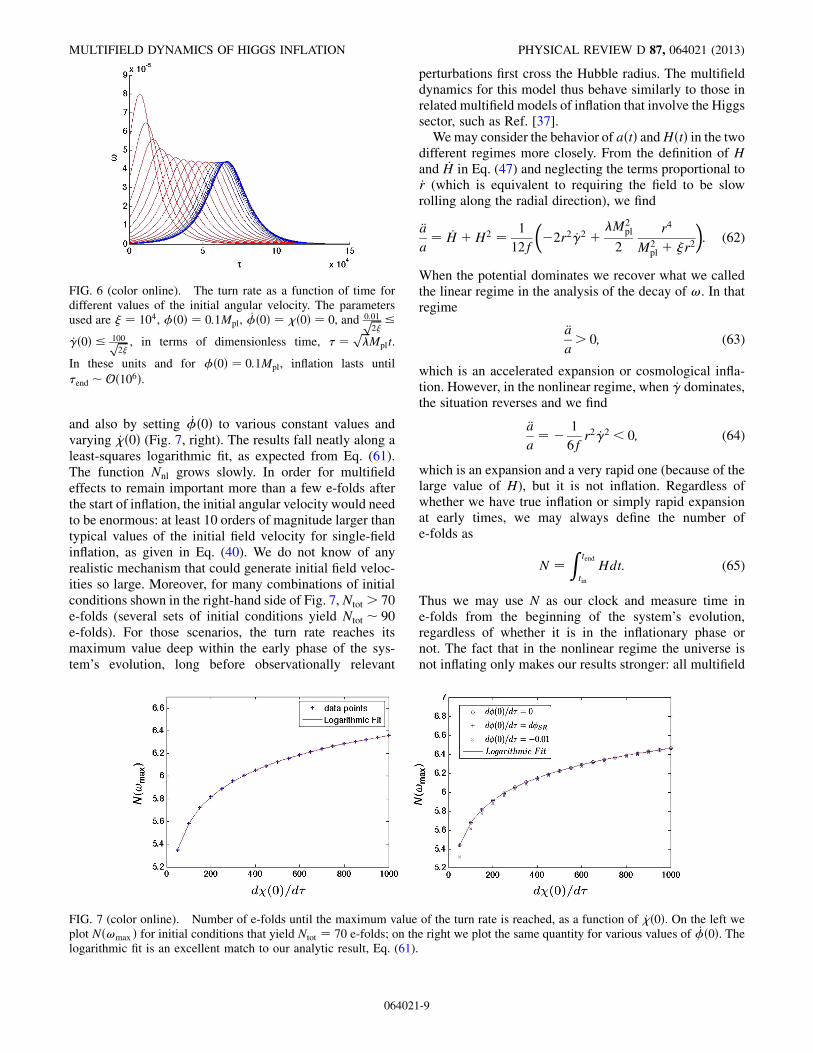
We have verified all of these analytic predictions usingnumerical calculations of the exact equations for thecoupled two-field system in an expanding universe. InFig. 5 we plot the number of e-folds from the beginningof inflation at which the turn rate reaches its maximumvalue, as we vary the fields’ initial velocities. Note that forany combination of initial conditions that yields at leastNtot ¼ 70 e-folds, ! reaches its maximum value betweenNð!max Þ ¼ 3:5 and 5 e-folds from the start of the fields’evolution (for the range of initial conditions consideredthere). In Fig. 6 we plot ! as a function of time as we varythe initial angular velocity, _�ð0Þ. The curves in red corre-spond to initial conditions in the linear regime, while thecurves in blue start in the nonlinear regime. Note that the

curves starting in the nonlinear regime have the sameamplitude. The existence of a maximum time, tnl;max , is

evident from the bunching of the blue curves. We findffiffiffiffi

pMpltnl;max ¼ �nl;max � few� �� 104, as expected

from Eq. (60). In these units and for the initial conditionsused in Fig. 6, inflation lasts until �end �Oð106Þ, so �nl;max

occurs very early after the onset of inflation.Equation (55) shows that the linear region lasts at most

a few e-folds, so the duration of the nonlinear region iswhat will ultimately determine whether or not multifieldeffects will persist until observationally relevant lengthscales first cross the Hubble radius. In the nonlinear re-gime, Eq. (52) yieldsH ’ _�=

ffiffiffiffiffiffi6�

pwith _� given by Eq. (57).

The number of e-folds for which the nonlinear regimepersists is given by

Nnl¼Z tnl

0Hdt’ 1ffiffiffiffiffiffi

6�p

Z tnl

0_�dt¼1

3ln

0@ ffiffiffiffiffiffi

2�

s_�0

Mplz

1A: (61)

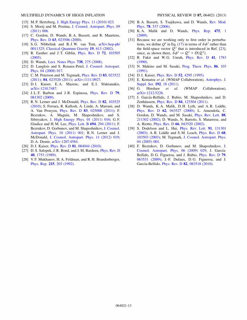
We examine Eq. (61) numerically by fixing � ¼ 104 and�ð0Þ ¼ 0:1Mpl and choosing pairs of initial velocities,_�ð0Þ and _ð0Þ, which yield 70 e-folds (see Fig. 7, left),

FIG. 5 (color online). Contour plots showing the number of e-folds at which the maximum of the turn rate occurs, as one varies thefields’ initial conditions. In each panel, the vertical axis is _ð0Þ and the horizontal axis is _�ð0Þ. The panels correspond to �ð0Þ ¼10�1Mpl (top left), 10�2Mpl (top right), 5� 10�3Mpl (bottom left), and 10�4Mpl (bottom right). We set � ¼ 104 and use the

dimensionless time variable � ¼ ffiffiffiffi

pMplt. The thick black curve is the contour line of initial conditions that yield N ¼ 70 e-folds.

GREENWOOD, KAISER, AND SFAKIANAKIS PHYSICAL REVIEW D 87, 064021 (2013)

064021-8

and also by setting _�ð0Þ to various constant values andvarying _ð0Þ (Fig. 7, right). The results fall neatly along aleast-squares logarithmic fit, as expected from Eq. (61).The function Nnl grows slowly. In order for multifieldeffects to remain important more than a few e-folds afterthe start of inflation, the initial angular velocity would needto be enormous: at least 10 orders of magnitude larger thantypical values of the initial field velocity for single-fieldinflation, as given in Eq. (40). We do not know of anyrealistic mechanism that could generate initial field veloc-ities so large. Moreover, for many combinations of initialconditions shown in the right-hand side of Fig. 7, Ntot > 70e-folds (several sets of initial conditions yield Ntot � 90e-folds). For those scenarios, the turn rate reaches itsmaximum value deep within the early phase of the sys-tem’s evolution, long before observationally relevant

perturbations first cross the Hubble radius. The multifielddynamics for this model thus behave similarly to those inrelated multifield models of inflation that involve the Higgssector, such as Ref. [37].Wemay consider the behavior of aðtÞ andHðtÞ in the two

different regimes more closely. From the definition of Hand _H in Eq. (47) and neglecting the terms proportional to_r (which is equivalent to requiring the field to be slowrolling along the radial direction), we find

€a

a¼ _H þH2 ¼ 1

12f

��2r2 _�2 þ M2

pl

2

r4

M2pl þ �r2

�: (62)

When the potential dominates we recover what we calledthe linear regime in the analysis of the decay of !. In thatregime

€a

a> 0; (63)

which is an accelerated expansion or cosmological infla-tion. However, in the nonlinear regime, when _� dominates,the situation reverses and we find

€a

a¼ � 1

6fr2 _�2 < 0; (64)

which is an expansion and a very rapid one (because of thelarge value of H), but it is not inflation. Regardless ofwhether we have true inflation or simply rapid expansionat early times, we may always define the number ofe-folds as

N ¼Z tend

tin

Hdt: (65)

Thus we may use N as our clock and measure time ine-folds from the beginning of the system’s evolution,regardless of whether it is in the inflationary phase ornot. The fact that in the nonlinear regime the universe isnot inflating only makes our results stronger: all multifield

FIG. 7 (color online). Number of e-folds until the maximum value of the turn rate is reached, as a function of _ð0Þ. On the left weplot Nð!max Þ for initial conditions that yield Ntot ¼ 70 e-folds; on the right we plot the same quantity for various values of _�ð0Þ. Thelogarithmic fit is an excellent match to our analytic result, Eq. (61).

FIG. 6 (color online). The turn rate as a function of time fordifferent values of the initial angular velocity. The parametersused are � ¼ 104, �ð0Þ ¼ 0:1Mpl, _�ð0Þ ¼ ð0Þ ¼ 0, and 0:01ffiffiffiffi

2�p

_�ð0Þ 100ffiffiffiffi2�

p , in terms of dimensionless time, � ¼ ffiffiffiffi

pMplt.

In these units and for �ð0Þ ¼ 0:1Mpl, inflation lasts until

�end �Oð106Þ.

MULTIFIELD DYNAMICS OF HIGGS INFLATION PHYSICAL REVIEW D 87, 064021 (2013)

064021-9

effects decay before the observable scales exit the horizonin a model that produces enough inflation to solve thestandard cosmological problems.

As a final test of our analysis we set � ¼ 102 instead of� ¼ 104. The smaller value of the nonminimal couplingdoes not lead to a viable model of Higgs inflation—theWMAP normalization of the power spectrum requires alarger value of � [5]—but we may nonetheless study thedynamics of such a model. We collect the important infor-mation about the dynamics of this model in Fig. 8. Asexpected, the model can provide 70 or more e-folds ofinflation for a wide range of parameters, and the corre-sponding turn rate peaks well before observationally rele-vant length scales first crossed the Hubble radius, even

when we increase _ð0Þ to a few hundred in units of � ¼ffiffiffiffi

pMplt. The excellent logarithmic fit of the time at which

the turn rate is maximum versus _ð0Þ is again evident.Finally the curves of the turn rate versus time show thesame qualitative and quantitative characteristics as Fig. 6for � ¼ 104. Specifically, if one rescales time and the turn

rate appropriately by �, the two sets of curves would behardly distinguishable.

V. IMPLICATIONS FOR THEPRIMORDIAL SPECTRUM

We have found that in models with an SOðN Þ symme-try among the scalar fields, the turn rate quickly damps tonegligible magnitude within a few e-folds after the start ofinflation. In this section we confirm that such behavioryields empirical predictions for observable quantities likethe primordial power spectrum of perturbations that repro-duce expectations from corresponding single-field models.For models that behave effectively as two-field models,

which include the class of SOðN Þ-symmetric models weinvestigate here, we may distinguish two scalar perturba-tions: the perturbations in the adiabatic direction, Q�

defined in Eq. (18), and a scalar entropic perturbation [23],

Qs � !I

!�sI: (66)

FIG. 8 (color online). Dynamics of our two-field model with � ¼ 102, �ð0Þ ¼ 1Mpl, and ð0Þ ¼ 0. Clockwise from top left:(1) Contour plot showing the number of e-folds as one varies the fields’ initial conditions. The thick curve corresponds to 70 e-folds.(2) Contour plot showing the number of e-folds at which the maximum of the turn rate occurs, as one varies the fields’ initialconditions. The thick curve corresponds to Ntot ¼ 70 e-folds. (3) Number of e-folds until the maximum value of the turn rate is reachedfor initial conditions giving Ntot ¼ 70 e-folds, along with a logarithmic fit. (4) The turn rate as a function of time for different values ofthe initial angular velocity, with _�ð0Þ ¼ 0 and 0:01ffiffiffiffi

2�p _�ð0Þ 100ffiffiffiffi

2�p , in units of � ¼ ffiffiffiffi

p

Mplt.

GREENWOOD, KAISER, AND SFAKIANAKIS PHYSICAL REVIEW D 87, 064021 (2013)

064021-10

We noted in Eq. (19) that Q� is proportional to the gauge-invariant curvature perturbation, Rc. We adopt a similarnormalization for the entropy perturbation,

S � H

_�Qs: (67)

In the long-wavelength limit, the adiabatic and entropicperturbations obey [23,38]

_Rc¼ HSþO�

k2

a2H2

�; _S¼�HSþO

�k2

a2H2

�; (68)

so that we may define the transfer functions

TRSðt; tÞ ¼Z t

tdt0 ðt0ÞHðt0ÞTSSðt; t0Þ;

TSSðt; tÞ ¼ exp

�Z t

tdt0�ðt0ÞHðt0Þ

�:

(69)

We take t to be the time when a fiducial scale of interestfirst crossed the Hubble radius during inflation, defined bya2ðtÞH2ðtÞ ¼ k2. In Ref. [23], we calculated

ðtÞ ¼ 2!ðtÞHðtÞ (70)

and

�ðtÞ ¼ �2�� �ss þ ��� � 4

3

!2

H2; (71)

where � � � _H=H2 and the other slow-roll parameters aredefined as

��� � M2pl

M��

V; �ss � M2

pl

!I!JMI

J

!2V: (72)

The dimensionless power spectrum is given by

PR ¼ k3

2�2jRcj2 (73)

and hence, from Eqs. (68) and (69),

PRðkÞ ¼ PRðkÞ½1þ T2RSðt; tÞ�; (74)

where k corresponds to a length scale that crossed theHubble radius at some time t > t. The spectral index isthen given by

nsðtÞ ¼ nsðtÞ � ½ ðtÞ þ �ðtÞTRSðt; tÞ� sin ð2�Þ; (75)

where

cos� � TRSffiffiffiffiffiffiffiffiffiffiffiffiffiffiffiffiffiffiffi1þ T2

RS

q : (76)

In the limit ð!=HÞ � ���, the spectral index evaluated atN assumes the single-field form [29,30,34],

nsðtÞ ¼ 1� 6�ðtÞ þ 2���ðtÞ: (77)

Crucial to note is that the turn rate, !, serves as awindow function within TRSðt; tÞ: once the coefficient

¼ 2!=H becomes negligible, there will effectively beno transfer of power from the entropic to the adiabaticperturbations, much as we had found by examining thesource terms on the right-hand sides of Eqs. (20) and (21).The question then becomes whether !ðtÞ, and henceTRSðt; tÞ, can depart appreciably from zero at timeswhen perturbations on length scales of observational inter-est first cross the Hubble radius.The longest length scales of interest are often taken to be

those that first crossed the Hubble radius N ¼ 55� 5e-folds before the end of inflation [28–30]. Closer analysissuggests that length scales that first crossed the Hubbleradius N ¼ 62–63 e-folds before the end of inflationcorrespond to the size of the present horizon [39].Meanwhile, we follow [29] in assuming that successfulinflation requiresNtot � 70 e-folds to solve the horizon andflatness problems. The question then becomes whether!ðtÞ, and hence TRSðt; tÞ, can differ appreciably fromzero for N 63. Given the analysis in Sec. IV, the bestchance for this to occur is for initial conditions that pro-duce the minimum amount of inflation, Ntot ¼ 70.In Table I, we present numerical results for key measures

of multifield dynamics. In each case we set � ¼ 104,�ð0Þ ¼ 0:1Mpl, and ð0Þ ¼ 0. We vary _ð0Þ as shown

and adjust _�ð0Þ in each case so as to produce exactlyNtot ¼ 70 e-folds of inflation. Because TRS remains sosmall in each of these cases, there is no discernible runningof the spectral index within the window N ¼ 63 toN ¼ 40 e-folds before the end of inflation. If we considera fiducial scale k that first crosses the Hubble radius atN ¼ 63 e-folds before the end of inflation, then we findns ¼ 0:97 across the whole range of initial conditions,in excellent agreement with the measured value of ns ¼0:971� 0:010 [36]. If instead we set k as the scale thatfirst crossed the Hubble radius N ¼ 60 e-folds before theend of inflation, we find ns ¼ 0:967 across the entire rangeof initial conditions, again in excellent agreement with thelatest measurements.

VI. CONCLUSIONS

In this paper we have analyzed Higgs inflation as amultifield model with nonminimal couplings. Becausethe Goldstone modes of the Standard Model electroweak

TABLE I. Numerical results for measures of multifield dy-namics for Higgs inflation with � ¼ 104. We use dimensionlesstime � ¼ ffiffiffiffi

p

Mplt.

_ð0Þ !ðN ¼ 63Þ TRSðmax Þ nsðN ¼ 63Þ nsðN ¼ 60Þ10�2 1:16� 10�10 2:68� 10�6 0.969 0.967

10�1 1:20� 10�9 2:76� 10�5 0.969 0.967

1 9:41� 10�9 2:18� 10�4 0.969 0.967

101 1:18� 10�7 2:72� 10�3 0.969 0.967

102 1:12� 10�6 2:59� 10�2 0.973 0.967

MULTIFIELD DYNAMICS OF HIGGS INFLATION PHYSICAL REVIEW D 87, 064021 (2013)

064021-11

Higgs sector remain in the spectrum at high energies inrenormalizable gauges, we have incorporated their effectsin the dynamics of the model. Because of the high sym-metry of the Higgs sector—guaranteed by the SUð2Þ elec-troweak gauge symmetry, which manifests as an SOð4Þsymmetry among the scalar fields of the Higgs sector—thenonmiminal couplings for the various scalar fields takeprecisely the same value (�� ¼ � ¼ �), as do the tree-

level couplings in the Jordan-frame potential (� ¼ ¼, and so on). The effective potential in the Einstein frametherefore contains none of the irregular features, such asbumps or ridges, that were highlighted in Ref. [23] for thecase of multiple fields with arbitrary couplings. With nofeatures such as ridges off of which the fields may fallduring their evolution, Hubble drag will always cause anyinitial angular motion within field space to damp outrapidly. Increasing the initial angular velocity to arbitrarilylarge values—well into what we call the nonlinearregime—only increases the value of H at early times,which makes the Hubble drag even more effective andhence hastens the damping out of the multifield effects.

The rapidity with which the turn rate damps to zerocombined with the requirement of Ntot � 70 e-folds forsuccessful inflation means that the multifield dynamicsbecome negligible before perturbations on scales of obser-vational relevance first cross the Hubble radius. Even if wepush the observational window of interest back to N ¼ 63e-folds before the end of inflation, rather than the usualassumption ofN ¼ 55� 5, we find that the model relaxesto effectively single-field dynamics prior to N. Hence thepredictions from Higgs inflation for observable quantities,such as the spectral index of the power spectrum of pri-mordial perturbations, reduce to their usual single-fieldform. Moreover, the absence of multifield effects fortimes later than N means that this model should produce

negligible non-Gaussianities during inflation, in contrast tothe broader family of models studied in Ref. [23].The methods we introduce here may be applied to any

multifield model with nonminimal couplings and anSOðN Þ symmetry among the fields in field space. Theconclusion therefore appears robust that such highly sym-metric models should behave effectively as single-fieldmodels, at least within the observational window of interestbetween N ¼ 63 and N ¼ 40 e-folds before the end ofinflation. Of course, multfield effects could become im-portant in such models at the end of inflation, duringepochs such as preheating [40]. Such processes remainunder study.

ACKNOWLEDGMENTS

It is a pleasure to thank Alan Guth, Mustafa Amin, andLeo Stein for helpful discussions. This work was supportedin part by the U.S. Department of Energy (DOE) underContract No. DE-FG02-05ER41360.

APPENDIX: ANGULAR EVOLUTIONOF THE FIELD

For completeness, let us integrate the angular equationof motion, Eq. (53), for all values of _� (in the slow-rollregime of the radial field). This yields

_�ðtÞ� ffiffiffiffi

p

Mpl þffiffiffiffiffiffiffiffiffiffiffiffiffiffiffiffiffiffiffiffiffiffiffiffiffiffiffiffi2� _�2

0 þ M2pl

q �_�0

� ffiffiffiffi

pMpl þ

ffiffiffiffiffiffiffiffiffiffiffiffiffiffiffiffiffiffiffiffiffiffiffiffiffiffiffiffiffiffiffiffiffi2� _�2ðtÞ þ M2

pl

q � ¼ exp

��

ffiffiffiffiffiffi3

pMplt

2�

�:

(A1)

In the two limits, _�0 �ffiffiffiffi

pMpl=

ffiffiffiffiffiffi2�

pand _�0 �ffiffiffiffi

p

Mpl=ffiffiffiffiffiffi2�

p, we may solve Eq. (A1) and recover the forms

of �ðtÞ presented in Eqs. (55) and (57).

[1] ATLAS Collaboration, Phys. Lett. B 716, 1 (2012); CMSCollaboration, Phys. Lett. B 716, 30 (2012).

[2] D. H. Lyth and A. Riotto, Phys. Rep. 314, 1 (1999).[3] A. H. Guth and D. I. Kaiser, Science 307, 884 (2005).[4] A. Mazumdar and J. Rocher, Phys. Rep. 497, 85

(2011).[5] F. L. Bezrukov and M. E. Shaposhnikov, Phys. Lett. B 659,

703 (2008).[6] Y. Fujii and K. Maeda, The Scalar-Tensor Theory of

Gravitation (Cambridge University Press, Cambridge,

England, 2003).[7] V. Faraoni, Cosmology in Scalar-Tensor Gravity (Kluwer,

Boston, 2004).[8] N. D. Birrell and P. C.W. Davies, Quantum Fields in

Curved Space (Cambridge University Press, Cambridge,England, 1982).

[9] I. L. Buchbinder, S. D. Odintsov, and I. L. Shapiro,

Effective Action in Quantum Gravity (Taylor and

Francis, New York, 1992).[10] A. de Simone, M. P. Hertzberg, and F. Wilczek, Phys. Lett.

B 678, 1 (2009).[11] F. L. Bezrukov, A. Magnin, and M. E. Shaposhnikov, Phys.

Lett. B 675, 88 (2009); F. L. Bezrukov and M. E.

Shaposhnikov, J. High Energy Phys. 07 (2009) 089.[12] A. O. Barvinsky, A.Y. Kamenshchik, C. Kiefer, A. A.

Starobinsky, and C. F. Steinwachs, J. Cosmol. Astropart.

Phys. 12 (2009) 003; Eur. Phys. J. C 72, 2219 (2012).[13] S. Weinberg, The Quantum Theory of Fields, Modern

Applications Vol. 2 (Cambridge University Press,

Cambridge, England, 1996).[14] C. P. Burgess, H.M. Lee, and M. Trott, J. High Energy

Phys. 09 (2009) 103; 07 (2010) 007.

GREENWOOD, KAISER, AND SFAKIANAKIS PHYSICAL REVIEW D 87, 064021 (2013)

064021-12

[15] M. P. Hertzberg, J. High Energy Phys. 11 (2010) 023.[16] S. Mooij and M. Postma, J. Cosmol. Astropart. Phys. 09

(2011) 006.[17] C. Gordon, D. Wands, B. A. Bassett, and R. Maartens,

Phys. Rev. D 63, 023506 (2000).[18] S. G. Nibbelink and B. J.W. van Tent, arXiv:hep-ph/

0011325; Classical Quantum Gravity 19, 613 (2002).[19] R. Easther and J. T. Giblin, Phys. Rev. D 72, 103505

(2005).[20] D. Wands, Lect. Notes Phys. 738, 275 (2008).[21] D. Langlois and S. Renaux-Petel, J. Cosmol. Astropart.

Phys. 04 (2008) 017.[22] C.M. Peterson and M. Tegmark, Phys. Rev. D 83, 023522

(2011); 84, 023520 (2011); arXiv:1111.0927.[23] D. I. Kaiser, E. A. Mazenc, and E. I. Sfakianakis,

arXiv:1210.7487.[24] J. L. F. Barbon and J. R. Espinosa, Phys. Rev. D 79,

081302 (2009).[25] R. N. Lerner and J. McDonald, Phys. Rev. D 82, 103525

(2010); S. Ferrara, R. Kallosh, A. Linde, A. Marrani, andA. Van Proeyen, Phys. Rev. D 83, 025008 (2011); F.Bezrukov, A. Magnin, M. Shaposhnikov, and S.Sibiryakov, J. High Energy Phys. 01 (2011) 016; G. F.Giudice and H.M. Lee, Phys. Lett. B 694, 294 (2011); F.Bezrukov, D. Gorbunov, and M. Shaposhnikov, J. Cosmol.Astropart. Phys. 10 (2011) 001; R. N. Lerner and J.McDonald, J. Cosmol. Astropart. Phys. 11 (2012) 019;D. A. Demir, arXiv:1207.4584.

[26] D. I. Kaiser, Phys. Rev. D 81, 084044 (2010).[27] D. S. Salopek, J. R. Bond, and J.M. Bardeen, Phys. Rev. D

40, 1753 (1989).[28] V. F. Mukhanov, H.A. Feldman, and R.H. Brandenberger,

Phys. Rep. 215, 203 (1992).

[29] B. A. Bassett, S. Tsujikawa, and D. Wands, Rev. Mod.Phys. 78, 537 (2006).

[30] K. A. Malik and D. Wands, Phys. Rep. 475, 1(2009).

[31] Because we are working only to first order in perturba-tions, we define QI in Eq. (17) in terms of ��I rather thanthe field-space vector QI that is introduced in Ref. [23],since, as shown there, ��I ! QI þOðQ2Þ.

[32] R. Fakir and W.G. Unruh, Phys. Rev. D 41, 1783(1990).

[33] N. Makino and M. Sasaki, Prog. Theor. Phys. 86, 103(1991).

[34] D. I. Kaiser, Phys. Rev. D 52, 4295 (1995).[35] E. Komatsu et al. (WMAP Collaboration), Astrophys. J.

Suppl. Ser. 192, 18 (2011).[36] G. Hinshaw et al. (WMAP Collaboration),

arXiv:1212.5226.[37] J. Garcıa-Bellido, J. Rubio, M. Shaposhnikov, and D.

Zenhausern, Phys. Rev. D 84, 123504 (2011).[38] D. Wands, K.A. Malik, D.H. Lyth, and A. R. Liddle,

Phys. Rev. D 62, 043527 (2000); L. Amendola, C.Gordon, D. Wands, and M. Sasaki, Phys. Rev. Lett. 88,211302 (2002); D. Wands, N. Bartolo, S. Matarrese, andA. Riotto, Phys. Rev. D 66, 043520 (2002).

[39] S. Dodelson and L. Hui, Phys. Rev. Lett. 91, 131301(2003); A. R. Liddle and S.M. Leach, Phys. Rev. D 68,103503 (2003); M. Tegmark, J. Cosmol. Astropart. Phys.04 (2005) 001.

[40] F. Bezrukov, D. Gorbunov, and M. Shaposhnikov, J.Cosmol. Astropart. Phys. 06 (2009) 029; J. Garcıa-Bellido, D. G. Figueroa, and J. Rubio, Phys. Rev. D 79,063531 (2009); J.-F. Dufaux, D.G. Figueroa, and J.Garcıa-Bellido, Phys. Rev. D 82, 083518 (2010).

MULTIFIELD DYNAMICS OF HIGGS INFLATION PHYSICAL REVIEW D 87, 064021 (2013)

064021-13