multilabel learning for personalized bookmark classification · multilabel learning for...
TRANSCRIPT

Multilabel Learning forpersonalized BookmarkClassificationBachelor-Thesis von Bastian Christoph aus FritzlarApril 2014
Fachbereich InformatikFachgebiet Knowledge Engineering

Multilabel Learning for personalized Bookmark Classification
Vorgelegte Bachelor-Thesis von Bastian Christoph aus Fritzlar
1. Gutachten: Prof. Dr. Johannes Fürnkranz2. Gutachten: Eneldo Loza Mencia
Tag der Einreichung:
Bitte zitieren Sie dieses Dokument als:URN: urn:nbn:de:tuda-tuprints-12345URL: http://tuprints.ulb.tu-darmstadt.de/1234
Dieses Dokument wird bereitgestellt von tuprints,E-Publishing-Service der TU Darmstadthttp://[email protected]
Die Veröffentlichung steht unter folgender Creative Commons Lizenz:Namensnennung – Keine kommerzielle Nutzung – Keine Bearbeitung 2.0 Deutschlandhttp://creativecommons.org/licenses/by-nc-nd/2.0/de/

Erklärung zur Bachelor-Thesis
Hiermit versichere ich, die vorliegende Bachelor-Thesis ohne Hilfe Dritter nur mit den an-gegebenen Quellen und Hilfsmitteln angefertigt zu haben. Alle Stellen, die aus Quellenentnommen wurden, sind als solche kenntlich gemacht. Diese Arbeit hat in gleicher oderähnlicher Form noch keiner Prüfungsbehörde vorgelegen.
Darmstadt, den 20. April 2014
(B. Christoph)
1

Zusammenfassung
In dieser Ausarbeitung werden wir die Anwendung von Support-Vector-Machines für Multilabel hier-archical datasets zeigen, die über den allgemein bekannten Bookmark-Klassifikation-Prozess angelegtwurden. Dazu werden wir zwei Ansätze für die Multilabel-Klassifikation vorschlagen.Abschließend werden wir zeigen, dass die vorhergesagten Multilabel-Rankings für verschiedene levelsvon der Hierarchy evaluiert werden können.
Abstract
In this thesis we will show the application of support-vector-machines to multilabel hierarchical datasets,built in the commonly known process of bookmark classification. For this purpose we will propose twoapproaches for the multilabel classification.Finally we will show that the predicted multilabel rankings can be evaluated for the different levels ofthe hierarchy.
2
Contents
1 Introduction 4
2 Bookmark Classification and the System as Knowledge-Library 62.1 The TODO-List: Tab-based Browsing in Web Navigation . . . . . . . . . . . . . . . . . . . . . 82.2 Lifecycle: Different Phases of a Resource in the Knowledge Library . . . . . . . . . . . . . . . 82.3 Bookmark-Classification Process . . . . . . . . . . . . . . . . . . . . . . . . . . . . . . . . . . . . 102.4 Bookmarks-Tree . . . . . . . . . . . . . . . . . . . . . . . . . . . . . . . . . . . . . . . . . . . . . . 14
3 Multilabel Datasets 163.1 Newspaper: Chronologic Theme-Pages and Dossiers from the Meta-Catalogue . . . . . . . . 163.2 Reuters RCV1 V2 . . . . . . . . . . . . . . . . . . . . . . . . . . . . . . . . . . . . . . . . . . . . . 17
4 Data Preprocessing, Indexing 184.1 Wrappers for Service-Invocation-Outputs . . . . . . . . . . . . . . . . . . . . . . . . . . . . . . . 184.2 Reuters RCV1 V2 . . . . . . . . . . . . . . . . . . . . . . . . . . . . . . . . . . . . . . . . . . . . . 22
5 Multilabel Learning: Basic Modelling 235.1 Problem Formulation for Multilabel Classification . . . . . . . . . . . . . . . . . . . . . . . . . 235.2 Considerations, Problem Solving Strategy . . . . . . . . . . . . . . . . . . . . . . . . . . . . . . 245.3 Hierarchy Decomposition, Binary Relevance Decomposition . . . . . . . . . . . . . . . . . . . 265.4 Multilabel Classifier Training . . . . . . . . . . . . . . . . . . . . . . . . . . . . . . . . . . . . . . 305.5 Classifier Predictions, Bipartition, Label Ranking . . . . . . . . . . . . . . . . . . . . . . . . . . 315.6 Test Instance Prediction, Exploration of the trained Hierarchy . . . . . . . . . . . . . . . . . . 32
6 Multilabel Learning: Approaches 346.1 Approach 1: 1-Level, flat Tree (Binary Relevance) . . . . . . . . . . . . . . . . . . . . . . . . . 346.2 Approach 2,3: Multi-Level, hierarchical Tree (HOMER) . . . . . . . . . . . . . . . . . . . . . . 34
7 Experiments 357.1 Evaluation Levels . . . . . . . . . . . . . . . . . . . . . . . . . . . . . . . . . . . . . . . . . . . . . 357.2 Evaluation Measures . . . . . . . . . . . . . . . . . . . . . . . . . . . . . . . . . . . . . . . . . . . 367.3 Setup . . . . . . . . . . . . . . . . . . . . . . . . . . . . . . . . . . . . . . . . . . . . . . . . . . . . 38
7.3.1 Configuration of the Classifier . . . . . . . . . . . . . . . . . . . . . . . . . . . . . . . . . 397.3.2 Configuration of the Hierarchy-Exploration . . . . . . . . . . . . . . . . . . . . . . . . . 397.3.3 Approach 1 . . . . . . . . . . . . . . . . . . . . . . . . . . . . . . . . . . . . . . . . . . . . 407.3.4 Approach 2,3 . . . . . . . . . . . . . . . . . . . . . . . . . . . . . . . . . . . . . . . . . . . 40
8 Evaluation 418.1 Approach 1 . . . . . . . . . . . . . . . . . . . . . . . . . . . . . . . . . . . . . . . . . . . . . . . . . 428.2 Approach 2 . . . . . . . . . . . . . . . . . . . . . . . . . . . . . . . . . . . . . . . . . . . . . . . . . 448.3 Approach 3 . . . . . . . . . . . . . . . . . . . . . . . . . . . . . . . . . . . . . . . . . . . . . . . . . 468.4 Approach 1 vs. 2 . . . . . . . . . . . . . . . . . . . . . . . . . . . . . . . . . . . . . . . . . . . . . . 488.5 Approach 2 vs. 3 . . . . . . . . . . . . . . . . . . . . . . . . . . . . . . . . . . . . . . . . . . . . . . 48
9 Conclusions, Further Work 49
3

1 Introduction
Over multiple years, a large size of web-portals developed, providing their content to different groups ofusers.
As each content-provider usually focuses on specialized fields of knowledge, they developed schemesof resource-classification in terms of content-management-systems, underlying the portal to manage thedelivery of new published items, which are often inspired by the traditional news-publishing-schemesknown from the field of journalism.
As users usually read across the internet over multiple sources, they develop over browsing- andreading-sessions an own view of which content-providers share the most relevant content, such thatusers revisit the portals again when looking for new up-to-date content.
When managing their known and read resources, users apply the technique of storing shortcut-descriptors of the resources as bookmarks to their bookmark-knowledge-library, organized usually flatbut partially hierarchical in bookmark folders, building an own library-catalogue-scheme.
Over sessions, it can be observed, that users build their own organization and classification schemefor their shortcut-library, mostly build out of the processed content. It is also partially influenced by thecontent-management-metadata, explicitly shared by the content providers. This can be distinguishedheadlines, breadcrumbs or expanded url-paths including natural language words, used in direction for agood orientation in content and a good usability-experience, such that users can easily point to that overtechniques like bookmarks and have an orientation to come back on information needs and search overwidely known web-search-interfaces, using the remembered focused vocabulary.
In this thesis, we will show the application of approaches from the field of machine learning, to sup-port the user with a multi-label ranking, based on the user-defined methodology-scheme of organizingbookmarks into a hierachical folder-class structure.
First we will show how the process of bookmark classification during tabbed-browsing on user- interac-tion can be modelled and where we can take advantage of our classification approach to support the user.
There we will describe, how webresources from different content-providers can be represented in alibrary-catalogue over indexing.In that phase of preprocessing, the basic elements are registered to later build vectors of features for thetraining of a classifier.For that we will take a short look at the organization-scheme of content-providers, named theme-pagesor dossiers, where items are grouped by an identified theme-category under a specific name to cover inabstract the content-topics of the item-subsets.
Second we will discuss the training of a linear support vector machine classifier to build a basis forbinary-relevance (br) predictions of items coming additionally in the testing / prediction step.There we build for each folder-class a br classifier, which classifies in a one-against-all fashion the class-instances against the set of instances over all of the remaining folder-classes.
In the third section we will use the results from the set of br-classifiers to calculate for each newincoming item-instance a personalized (personal library based) ranking of the best suitable classes for
4

the instance, where we want to support a user in assigning one new instance to more than just oneclass (multi-label), since often users find themselves in the situation, that content-items cover from theirown point of personal qualification, evolved chronological knowledge and target interest on informationneeds, multiple subtopics, that will be found in multiple folders, building an intersection of differentfields of knowledge, that can later be a basis, to split or merge/cluster the folders, leading to a moredistinguished classification-scheme.There, users are mapping topics of interest over item-sets, best to their recent professional and chrono-logical knowledge, to a hierarchically organized folder-structure with an assigned focused, controlledvocabulary behind it.As goal of distinguishing the personal classification-scheme over sessions, it can be observed that usersreach a better focused vocabulary, leading to more precise navigation in the web, on interactions withsearch-interfaces, as feedback results do better cover the goal of information seeking, the more precisethe typed keywords were selected.
In Chapter 3 we show our multilabel datasets and which issues should be considered in contrast to thewidely known social bookmark classification techniques.
In Chapter 4 we show the important aspect of focusing towards the article-content directly and howthis is used to build our indexing of the datasets in the database.
In Chapter 5 we formulate the connection to the field of machine learning, how the imported datasetscan be decomposed for the learning of classifiers and how classifiers are used for multilabel classificationand label ranking of the predicted results.
In Chapter 6 the experiments running on the two datasets are proposed, especially how flat single-level bookmarks and hierarchical multi-level bookmarks can be covered using our approach. There wewill basically address the class imbalance for a binary classification task.
In Chapter 7 we will show the general setup for the evaluation and the configurations for the experi-ments.
In Chapter 8 we evaluate the results of our experiments.
In Chapter 9 we finally summarize with our conclusions and show some suggestions for further work.
5
2 Bookmark Classification and the System as Knowledge-Library
When users are exploring the web over browsing tasks and browsing sessions, they get experience withthe websites to judge about the content and functionality. As some of the explored websites often fit theinformation needs of the users, they are revisiting these websites.
Service Library Catalogue
The websites can be treated as services with specific functionality. All the websites, that one user isexploring regularly, can be treated as his ’Service Library Catalogue’.
Content Library Catalogue
When a user is opening an URL in the browser, he retrieves mostly an HTML-document as answer for aGET-request. This can be treated as the content-output of the invocation of the URL as service-function.To build an index over these content, we need to apply wrappers, that select the needed parts of theHTML-document and store these as reduced, distinguished representation in the database.
The distinguished datasets in the database are building the ’Content Library Catalogue’ and areneeded to define the features for the training of algorithms to calculate automatic recommendations forbuilding a personalized classification scheme.
This type of focusing on the content-reading is known from browsing tools like Readability1, the Safari-Reading-Mode2 or the iReader-Plugin3 for Firefox and Chrome. These are usually invoking the functionover a Bookmarklet.
Reference Library Catalogue
As third point, the user is usually reminding important or useful HTML-documents over storing the URLtogether with some parts of metadata-text as shortcut-descriptor (Bookmark) and organizes these ref-erences in a hierarchical tree structure, as bookmarks are assigned to bookmark-folders and bookmark-folders can have other bookmark-folders as parent.
This tree-structure does not contain the HTML-documents or content inside the documents itself andso we will call it the ’Reference Library’.
Since one bookmark can be added multiple times to the tree for different folders, we can consider thewhole bookmarks-tree as multilabel dataset, where the descriptor of a folder-node is called ’Label’ andthe sparse feature vector generated out of the content-output is called ’Instance’.
1 http://www.readability.com/2 http://support.apple.com/kb/PH5068?viewlocale=en_US3 http://samabox.com/extensions/iReader/
6
In terms of browsing tools, currently read-later and aggregation tools like Instapaper4, Pocket (ReadIt Later)5, Readability6, Evernote Clearly7, Storify8, Pinboard9 are available.
Personal read-only View of the Web, Labeling Vocabulary, Focused Vocabulary
The user is usually storing only shortcuts to web-pages, where the HTML-document itself behind theinvocation of the URL is almost static, since the idea of bookmark classification is to map the process offinding and reminding [1] large sets of web pages into the bookmark organization tool. This has alsobeen considered in [2], following the concept of associative linking [3].So we want to assume, that the user is building a personal view of the web [4] over browsing sessionsand encodes his knowledge partially over organizing the shortcut-references in the bookmarks-tree.In the bookmark-folder-descriptors the user is defining personal words (labeling words) that should bea super-concept in relation to the descriptor-words of the contained bookmark-set. There the focusedvocabulary, that is selected by the user to make the assignment, usually not formulated explicitly.In that case, it can be assumed, that these modeling of knowledge organization does apply to a read-onlytype of the web. The only type of writing is when the user types special values as invocation-parametersof services on HTTP-GET, which can be stored to logfiles on the server side.
As the user is naming the bookmark-folders based on his knowledge about the bookmarked items andproperties shared across sets of bookmarks, the used words for naming can be treated as labeling vocab-ulary. The knowledge here is about selecting a focused vocabulary out of the webresource words andfind words from the folder-labeling-vocabulary to make the mapping.
If two bookmark-folders share a common set of bookmarks it can be considered, that the bookmark-folder-concepts are related / associated with each other in terms of co-occurence. This has been exam-ined in the Associative Read-Out Model (AROM) in [5], using an associative layer [6].The associative relation between words has early been discussed in [7].
It can be observed as a goal, that the user is learning (building) a structured scheme in type of anontology, related to a library catalogue [8] of a digital library [9].
4 http://www.instapaper.com/5 http://getpocket.com/6 http://www.readability.com/7 http://evernote.com/intl/de/8 http://storify.com/9 http://pinboard.in/
7

2.1 The TODO-List: Tab-based Browsing in Web Navigation
Each tab in the browser can be treated as an entry on the TODO-list of the user in a web navigationsession. With a growing amount of opened tabs, the user has a growing TODO-list. For a growingTODO-list, the user needs to define priorities for the entries, where the number of priorities can bedefined with a range, such that multiple entries can have the same priority. Entries with an identicalpriority are defining an entry-group. Each group of tabs in tabbed browsing can be moved to a separatebrowser-window.In organization of the TODO-list the user can assign self-defined concepts / labels to the priorities inorder to remind the groups over natural-language words instead of the priority-numbers. Additionallythe natural-language words are usually formulated related to the meta-data of the tabs in the tab-group,that the user can see in organisation, without going into the document-content itself.This gives us a first labeling-intention for the later formulation of bookmark-folders for a group of book-marks.
2.2 Lifecycle: Different Phases of a Resource in the Knowledge Library
When the user draws resources out of the web, usually different steps are done in order to do a bookmarkclassification process. Especially in browser-interaction links are first opened in new tabs, later added asbookmark and get further classified in hierarchical organization. Here we want to show the lifecycle firstto give a basic understanding for our modelling in this thesis.After that we will show the browser-interaction process to point out at which step we want to takeadvantage for our approach to support the user there.
1. Discoverable:
Initially the article is not published and not available on the web.
a) Adressable:
In the publishing phase, the each page of the article is assigned as HTML document to an URL.Therefore the article gets adressable over the URL or set of URLs in type of a ’Web Resource’.In Section 4.1 we will further describe how a multi-document article can be handled.
b) Accessible:
When the article was assigned to an URL, it is still only reachable for those, who know theURL. Therefore it needs to be integrated into the website navigation structure over placinglinks to the URL on different documents that are still accessible. With that the web resourceis accessible over a navigation path. In the case of search engines, a crawler can retrieve theresource over a navigation path now and adds it then with the document-text-unit (token)-representation to an index. Therefore the resource gets accessible over the resultset of theinvocation of a search query, related to the indexed documents.
2. Observed:
When the user navigates on browsing through the websites or applies search queries, he can dis-cover resources along the path. When the user now decides to open the dicovered resource in anew browser tab, we define, the resource was actively ’observed’.Here, the user read only the metadata (url, page-title, headline, date) of the resource withoutfurther investigation.
3. Structurable:
During browsing sessions users often want to remind some of the observed resources when theyare clearly ’important’ or maybe ’needed’ with respect to a specific context. Therefore users can
8

simply add them as bookmarks to the root of the bookmarks-tree or there needs to exist a specificbranch (structure) on a growing tree, such that the user can easily remind, to search on which pathof the tree to reach these reminded bookmarks.
For that structure we can identify two prototypes. At first the structure is formulated before thebookmark is added. In the second case some bookmarks are collected under the root node andwhen the user has a specific need for organization, a branch is created. We will later discuss theseprototypes more in detail.
4. Collected:
When the user decides to add the observed article at least to the root node of the bookmarks-treethe article gets ’collected’.This is comparable to the user sending an email with links to himself to collect it in the ’TO_READ’-named email-folder.Here the user decided to include the article to his library without explaination. The content of thearticle may get important, when a larger set of items has been collected.
5. Organized:
With a growing set of collected bookmarks the user gets a need to further distinguish between sub-sets inside a growing collection. Therefore the subsets are assigned in organization to a preparedstructure-branch. Now the user can easier remind the distinguished subsets over the tree-structure.Here, additionally to the metadata, the user was reading parts of the content of the article. Thiscan be summary / first paragraph, some paragraphs starting at the beginning or the first page ofa multi-page article. With that action, the article was further classified through adding additionalcontext information (folder description in the browser profile). We define the article was set intoa personal context by the user. Here the user needs to read at least parts of the content to judgeabout which folder should be selected. When no specified folder can be determined, the root nodeof the current browser profile (e.g. ’Home’, ’Work’, ’University’, ’Development’) is used as basiccontext. We will later discuss an approach, how the user can be supported in finding a suitablefolder in his environment, based on his personally built tree.
9

2.3 Bookmark-Classification Process
In this section we want to show the general process of bookmark classification to give a basic under-standing at which steps we can take advantage of our approach to support the user in the process.
At first we will show the steps in the process.
1. Define a browsing-task as browsing-context:
Usually the user finds himself in a specific context as starting point, why a browsing session shouldbe done. This context can be e.g. location, project, task group, task.
Here we can especially observe, that a single person is usually having a user-account on multipleclient-computers (e.g.: at home, at work, mobile-devices), which means that the user-profile canbe distributed over multiple clients and one machine-user can have multiple web browser profiles,each assignable (usable) for a special context.
As the user can be in different and changing working contexts when building the bookmarks-treewe can assume, that he is building it in a ’self-collaborative’ way.
For a general location-context, a browsing-task can be formulated like ’Which articles are new formy topics of interest at my sources of interest?’
This gives the constraints for the initial task-context:
• retrieve articles as HTML documents
• the articles are most recent to the current date
• the topics of interest are mostly formulated abstract and are to be specified more precisely dur-ing browsing over formulating words that the user knows from his general labeling-vocabulary
• the sources of interest are personally selected / acceptable / trusted websites
When working on a project and solving groups of tasks or a single task the formulation what to besearched is usually more specific.
2. Start the browsing-session:
Start the browser and open the first window over selecting a web browser profile.
3. Observe: Open resources, that seem to be relevant for the problem-solving of the browsing-task:
Navigate through the known websites and open pages in new tabs, that contain words, relevant tothe topics of interest.
Here it can often be observed, that as current websites have an underlying content managementsystem, approaches are used to recommend also pages to the user, that are in any type similar withor related to the opened one, relevant for the task.
There users often open pages from these clustered recommendation, that do not match the brows-ing task directly and are relevant to these, but are related to that task over the organization schemeof the content management system.
10
An example for this are side-recommendations like ’new in the ressort / category’, ’most read’,’most commented’ or ’users who read this, also read ...’.
This effect, also known from browsing (walking) through a library, where users find books not bydirect search, but by the order of the bibliographic organization scheme in position next to thesearched one, is often called ’Serendipitious Information Encountering’ [10].
In this case it needs to be considered, that the user is in fact unconsciously extending his formula-tion of the browsing task, when opening pages, that where initially not thought to be opened andnot matchable over the initial formulation.
Here a type of noise is introduced, compared with the initial task. This often leads the user intolosing increasingly the overview over the several adressed topics [11] across the growing collec-tion of pages when switching often between them. It is often considered as ’Information Over-load’ [12] [13] and sometimes as ’Organization Underload’ [14] as the user loses increasingly theability to distinguish between the contained subsets caused by their dissimilarity and missing ownorganization structures and adapts unconsciously to the organization scheme of the website [15]without explicitly accepting this by reformulating the personal scheme.
For the case, that the user wants to build a personal organization scheme that is applicable acrossmultiple websites and not only the current one, the user needs to get aware of his personal labeling-vocabulary for an abstract formulation of his topics in order to learn a strategy for a focused navi-gation.
As approach to solve this, the user needs to explicitly formulate an organizational structure ofgroups of pages, where each group is assigned a focused vocabulary to get the ability back to for-mulate explicitly central assumptions about the topics, covered by each group of pages, underlyingthe growing collection.
With the increasing availability of content with the growing web, it becomes a need for the usersto develop a personal formulation, which recommendations of the available websites should beincluded and which ones are not relevant, related to that personal organizational scheme.
This should give a method for a more structured, focused navigation with a continously growingweb, considered in abstraction as a type of digital library. Thereby a personal catalogue shouldhelp to do the classification and filtering.
It can be thought to include the personal scheme for reducing the views of the websites to pages,that are matchable with the vocabulary behind the personal scheme, reducing negative effects ofserendipitious information encountering and leading to a more focused navigation in the web.
In terms of web crawling, the personal catalogue can also be used in personalization as referencefor a schema-based focused crawler [16].
4. Pre-collect: Group the opened resources over tabbed browsing workspace
Here the goal can be observed to formulate groups of tabs to find suitable folders for sets ofbookmarks in a session of parallel browsing [17].
11

a) Build groups of resources (implicit group vocabulary):
Create an additional window, that should represent the group. The window is initially as-signed the known, defined browsing-task. As the group-window should cover a subset of theresources, we can formulate additional words as constraints in order to reach the reduction.
Now we move resources from the first window to the new one, that contains words fora shared specific topic. These words are first assumed to be added as constraints to thebrowsing-task-formulation and can be formulated temporally explicit in the window head.
This should give the user a strategy to build a frame for finding a formulation for the uncon-scious knowledge, applied for deciding to open the pages in the session of parallel browsing.There, the user wants to formulate a label-concept, such that all label-instances can be treatedas grouped by these label-concept.
b) Identify the group-vocabulary temporally explicit:
Switch to the new window, that contains the extracted group of resources. Here we find nowa reduced set of pages, compared to the initial task, as specific words were selected as addi-tional task constraints in order to identify the shared topic. Read the resources and identifyfrom each resource, which words should be assigned to the group temporally.
This can easily be done with a Tabbed-Browsing-Plugin like ’Tab Mix Plus’10, where words canbe added to the head of the Tab-Group-Window in the workspace view.
The words added to the tab-group-window are basically needed to distinguish the groups inthe overall workspace-view. After the resources are added later as bookmarks to the folders,these words can be discarded since the folder-label-words can be reminded.
5. Collect and organize the grouped resources
a) Structure: Create a bookmark-folder:
Create an empty folder-container and an empty folder-descriptor. Add the identified wordsfrom the group-vocabulary or related labeling-words to the descriptor.
b) Classify: Collect and organize the bookmarks:
Add all resources from the group as bookmark-shortcuts to the folder-container. This meansassigning each bookmark to the bookmark-folder.
Thereby the bookmark is the instance and the bookmark-folder is the instance-class, whenspeaking with the terms from machine learning. The user is here learning (training) a’instance-of’- relation (assignment), that should later be included as training data for theclassifier algorithm.In Chapter 5 we will further explain our modelling for multilabel-learning.
In the recent integrated browser-tools for assigning a bookmark to a bookmark-folder, e.g. thefirefox bookmarks, a ranking is presented to the user, that is based on which folder was usedby the user most recently and therefore sorted related to that. We define the ranking is forthat case sorted by the attribute ’recently used’.
10 https://addons.mozilla.org/de/firefox/addon/tab-mix-plus/
12

In this thesis we want to show a personalized approach, how a ranking can be generated, thattakes the webresource-content into account, which is delivered with the bookmark-HTML-document-sequence. Now an algorithm is trained with the user-bookmarks-tree based on thecontent and for a new bookmark as test-instance a ranking should be generated to supportthe user in the instance-assignment step. Additionally the ranking should recommend the firstfew folders as preselected to deliver a possible personalized multi-label assignment.
When the user is running browsing-sessions over time, it can be observed, that a resource,used for solving a previous browsing-task, can occur again for solving a different task.
In that case, a bookmark is assigned to multiple folders and can be considered as sharedacross multiple classes and shared across multiple tasks. In terms of machine learning, thisstep generates the bookmarks as ’Multi-Label Dataset’.
Hierarchical relation:When two bookmark-folders have a sufficiently large common set of bookmarks, the usercan decide to move that subset to a common parent. Therefore a new bookmark-folder iscreated and with it the empty folder-container and folder-descriptor. Then the common sub-set is moved from the child- containers to the parent-container. The common words fromthe child-descriptors are moved in reformulation to the parent-descriptor. Finally the newbookmark-folder is set as new parent to the child bookmark-folders and the previous parentof the child-folders is set as parent to the new folder, introducing a hierarchical relation forthe tree. This hierarchical subconcept-to-superconcept relation was considered in [18].Additionally this type of semantic relation was discussed as extension possibility for connec-tionist models [19], [7], [20].
13
2.4 Bookmarks-Tree
With the formulation of the process of bookmark classification, we have a structure for the organizationof references towards HTML-documents. As initially proposed in Section 2, we are considering thebookmarks-tree as ’Reference Library’, since these HTML-documents are the result, when invoking theservice when opening the URL, which is the representation of the service-function together with itsparameters for HTTP-GET. To give a basic unterstanding about how this reference library can be build,we want to show two prototypes of different organization strategies of the hierarchical structure, relatedto the lifecycle of the item.
Structure-Case: Early Hierarchy Formulation (Top Down)
When the user adds bookmarks, at first a suiting branch in the hierarchy must exist to assign book-marks there. If the branch does not exist, it needs to be build first. The created branches are usuallystructured related to the users professional experience with organizing documents in the general per-sonal ’Offline’ information management processes. This was especially examined in works about thepsychological issues [21] and the management of emails [12]. Additionally they are inspired by oftenfound organization schemes when browsing the web, for example ressort-categories or theme-pages fromnewspaper-websites or sitemaps in general. There the user does not know the underlying assumptions(rules) for the structure of the hierarchy-branches, but judges in imitation to agree with the structure andcopy it at least partially to the own knowledge-organization-hierarchy, extending his labeling-vocabulary.
With that, we can identify the sequence of operations from the lifecycle:
1. Structure:Build a suiting branch in the tree
2. Collect:Include the observed resource as bookmark to the reference library
3. Organize:Assign the collected bookmark to the bookmark-folder in the build branch
Structure-Case: Late Hierarchy Formulation (Bottom Up)
Here the user does initially not set hierarchy-rules and collects the bookmarks directly under the root-node in a type of ’pile’ [22], keeping in mind how to distinguish between different sets in the growingcollection. This is especially observed, when users only have a few bookmarks with no need for a morecomplex hierarchical organization. With a growing collection, the user needs to keep in mind increasingnumbers of subsets to distinguish between items and remind a sort order. For an increasing number ofsubsets, the user needs to formulate labeling-words explicitly, that are commonly shared across all itemsinside a subset of the collection. When each item is now assigned to a parent-folder in type of a ’prefix’using the formulated words, the user gets back a sort order over the collection, such that the differentsubsets can be distinguished easily. A hierarchy over multiple levels is built, when the prefixes are againprefixed with additional words. The hierarchy is usually visualized using a tree structure.
With that, we can identify the sequence of operations from the lifecycle:
1. Collect:Include the observed resource as bookmark to the reference library. It is assumed that it is assignedto the root-node.
14

2. Structure:If there are too much subsets in the collection under the root-node, identify one subset, define acommon attribute for that and build a folder (branch-structure) using that attribute.
3. Organize:Now the items from the identified subset have to be assigned there (moved from the root-nodetowards these new node). If the newly collected bookmark is not contained inside these item- set,it stays assigned under the root node.
Here we can observe, that this strategy is more directed to exclude easy formalizable subsets from theroot-node-collection than organizing the new bookmark directly to a folder in order to build a sortedtree-organization-structure. This gives us an explicit formulation of prior knowledge about growingcollections, just build out of the contained data and less oriented toward generally experienced variantsof possible hierachical organization. With respect to email-programs we would state here, that items arecollected in the root-inbox until the user is able to identify topics, that can be moved to a common folder,labeled with word-sets of each topic.
15

3 Multilabel Datasets
3.1 Newspaper: Chronologic Theme-Pages and Dossiers from the Meta-Catalogue
In the web, the availablility of user-generated hierachical bookmarks is usually quite low. Mostly, usersshare their bookmarks on folksonomy-like social bookmark classification services like delicious1, whichgives a flat one-level hierarchy without further explicit relations between tags.
There, conceptually users assign possibly multiple ’tags’ to a bookmark. When multiple users assigndifferent sets of tags to one resource in collaboration, only the resulting overall set of tags is shown.There the context-information about the used subset of tags is lost.In the definition of the tags it can usually be observed that a user is free to attach any word as tag toa bookmark and one tag is used by different users with varying background knowledge about a word,such that this polysemous usage of words leads to a type of noise [23].
To solve this, we will use an own created dataset, that is basically not build in a socially collaborativebut more self-collaborative way as we described in Section 2.2. In our case, we asssume that one proto-type user was building the dataset over multiple browsing sessions and possibly many client-machines.For the bootstrapping, we select so called ’Theme’-pages and ’Dossier’-pages, that will be imported by acrawler to some depth starting at the current date. Since one resource at a news portal can be assignedby the journalists in organization to multiple themes, this gives us a multi-label dataset.
In contrast to the concept of tagging we first allow, that one bookmark-folder-descriptor can havemultiple words. Second we allow that the user can formulate a hierarchy of folders, such that explicitparent-to-child relations can be defined.
As the user is usually reading across multiple news sites, we will pick possibly themes with the samename, available at different sites. In this point we abstract from the fact, that one special theme can behandled quite different, related to the journalistic main orientation of the editor-in-chief strategy behindthe site. There we ignore these possibly different fine-grained interpretation of themes and topics andtreat the overall merged theme as one bookmark folder.
These themes and dossiers are usually available in the meta-catalogue sections of the portals, whichgives the user easier and extended deeper access into the archive for a potentially increasing revisitation.The meta-catalogue feature can be found in news sites as Tagesschau Online23 , Spiegel Online4, FAZOnline5, ZEIT Online6, Golem Online7, Heise Online8, Computerwoche Online9 .
We can observe that similar to this meta-catalogue feature used in this newspaper websites, thebookmarks-tree is also based on the descriptive metadata of the web documents. In contrast thebookmarks-tree has an explicitly formulated hierarchical ordering relation for the folders, instead ofan alphabethical ordering relation in the newspaper websites.
1 https://delicious.com/2 http://meta.tagesschau.de/3 http://www.tagesschau.de/archiv/dossiers/4 http://www.spiegel.de/thema/5 http://www.faz.net/themen/6 http://www.zeit.de/schlagworte/themen/7 http://www.golem.de/specials/8 http://www.heise.de/thema/9 http://www.computerwoche.de/schwerpunkt/
16

Concept Drift
We can observe, that the interpretation of special theme-names and topic-names changes dependent onat which chronological point in time it is used.This is often called ’Concept Drift’ [24]. According to the incremental formulation of the bookmark-folder-descriptor we can observe, that a user introduces or reuses a word or set of words for each setof added bookmarks. Chronologically this sets give each a different meaning of the concept, such thatsubsets inside the folder define the drift in the concept.
For further investigation on concept drift it may get important to handle that overall single-label prop-erty inside the one folder as a multi-label property, as one single word can be used in multiple sets ofwords that are usually finally merged.
The concept drift is usually driven by the events in the calendar, where journalists have to report aboutthe current facts, happening in context with the theme at the selected calendar-dates. This is often usedin market-driven journalism [25] and online news production [26].
3.2 Reuters RCV1 V2
For our experiments we will use the benchmark dataset Reuters-RCV1-V2 [27] in its form available onthe website10.
This dataset was commonly used in lots of experiments inside the Information Retrieval (IR) andNatural Language Processing (NLP) Community, such that it is a good reference dataset to run our ex-periments for multilabel text classification.
10 http://jmlr.csail.mit.edu/papers/volume5/lewis04a/lyrl2004_rcv1v2_README.htm
17
4 Data Preprocessing, Indexing
4.1 Wrappers for Service-Invocation-Outputs
In recent observations about the structure of websites, it can be observed, that developers are increas-ingly following guidelines of good-case-practices to reach a better maintenance of the pages inside thewebsite and to make it more machine-readable for search-engine-optimization.
Content Management Systems, Abstract Template
It can be observed that with the increasing availability of open-source content-mangement-systems1 suchas Joomla, Drupal, TYPO3 and WordPress users can easily create personal websites or blogs. In general,developers are building some examples for a central, unified layout-template shared across all pagesinside a website-section. This will then be used to present all pages of the section in that layout to theuser, just filling in the template with the content, stored in the database-catalogue-tables. In many casesit can be observed, that developers do not always build the layout-templates themselves, but do morerely on the available frameworks for the management of content, increasingly available on the web,reducing the effort for an own distinguished webdesign.
Multi-Document Sequence, Central Content Filtering, Wrapper
When article-documents that are spanning over multiple pages are presented in the web, often one sep-arate HTML-document with an own URL for each document-page is created. Therefore using the firstURL only it can not be determined, if more HTML-documents exist in a sequence. If one user opens theURL and navigates through the document, a ’next’-link can sometimes be found that references to thenext document-page. Since each content-provider can encode that link in a different way, we have tobuild a special module called ’Wrapper’.
The wrapper should first implement a technique to read all URLs in the multi-document sequence. Sec-ond, each HTML-document is usually build out of multiple conceptionally different parts [15], such aswebsite-navigation, context information like breadcrumb, recommendations, central content and more.In this thesis we want to show an approach to train a classifier-algorithm based on the plain centralcontent inside the sequence of HTML-documents. Here we can especially observe that if we would useall words of the document sequence, then words from e.g. the navigation structure would be countedmany times if there are multiple documents in the sequence, resulting in misleading high word countersfor classifier-training. Therefore we have to implement a filter-approach [28] in the wrapper, that selectsthe special content-part out of the overall document.
Since we focus in this thesis on a manually essembled dataset, we do not implement wrappers for allwebsites in the web. In the case of adding a bookmark for a new website, a prototype wrapper can takejust the first document in the sequence and read all words from it. There we expect a type of trainingnoise, since if the user adds some documents of that website, the classifier would possibly get trained onthe often reoccurring words of the navigation structure.
Finally the resulting unified representation of the document generated by the wrapper should beregistered (stored) to the database. We want to call that unified representation ’Web Resource’.1 http://de.wikipedia.org/wiki/Content-Management-System
18
HTML Microdata, Semantic Web Data, Dublin Core Metadata
When looking at the DOM-representation of the pages, we can identify properties about the underlyingtemplates over looking at the (key, value) - pairs, delivered as attributes with the DOM-nodes.
There we can make use of three types of (key, value) - pairs:
• ’class’ attributeDevelopers often make use of the ’class’-attribute to outsource reoccurring CSS- layout and designinformation (style) to a separate CSS file and then encode the style over a special selected andpartially semantic meaningful name, put as value to the attribute to make the mapping. Whenusing this attribute, developers have the opportunity to format multiple areas of one page in thesame style and give identifying names to simplify the lookup.
• ’id’ attributeSome areas inside the template should be uniquely identifiable, such that developers make use ofthe ’id’-attribute, which can also be connected with a named CSS-style from an external file. Withthe increasing usage of that attribute, it becomes easier to select special elements (DOM-nodes)out of the DOM-tree representation. As these elements have an unique identifier, we can make amapping of the element-content over the ’getElementById’-method, widely supported in todaysDOM-reading-frameworks, to an element-variable in our abstract page-instance-representation.
• HTML MicrodataWith the upcoming HTML Microdata specification of the W3C2 and WHATWG3, it can be observedas a third point, that there is a standardization about attaching special names to the DOM-nodesas additional property-attributes, which are drawn from a specified general schema, used by thecontent provider to give a semantic enhancement, how the content inside the node should be in-terpreted.
As an example, the german news website SpiegelOnline4 adds for the article-area inside the news-item-page the attribute ’itemtype’ with the value Article5 to refer to the used schema in the section.Then the usage of the attribute-values (’datePublished’, ’headline’, ’author’, ’description’) can be ob-served for the attribute-key ’itemprop’, which leads to the assumption, that the content found thereshould be mapped to the article-fields (datePublished, headline, author, description/summary) inthe abstract representation as metadata, giving descriptive information about the article-instance.
As the formulation of node-microdata is analog to the formulation of class- and id-attribute, but moredirected to attach an explicit formulation over an additional schema-document, we will treat the valuesof the two last named property-attributes as ’Implicit Microdata’.
The technique of attaching a schema document is also currently known from the Semantic-WebResource-Description-Framework (RDF). Initiatives such as the Dublin Core Metadata Initiative (DCMI)6
are following the concept of building standardized vocabularies for such schemas.
2 http://www.w3.org/TR/2011/WD-microdata-20110525/3 http://www.whatwg.org/specs/web-apps/current-work/multipage/microdata.html4 http://www.spiegel.de5 http://schema.org/Article6 http://dublincore.org/
19

Wrapper Encoding, Indexing
For the generation of a webresource-instance, given the first URL, we need to build a wrapper for eachcontent-area (group of pages) for each website. This is analog to building a single wrapper or a group ofwrappers for each content-management-system.
For the encoding of each wrapper we need to make a static mapping-formulation that determines,which microdata- values should be used to map the text of the DOM-node to the related field of theabstract representation of the webresource.
Here we show a short example, how the summary-field of an article of the german news-websiteZeitOnline can be mapped (class=’excerpt’) using the Java-DOM-processing framework jsoup7:
/* (non-Javadoc)
* @see wrappers.IWrapper#extractSummary()
*/
@Override
public void extractSummary() {
String ressourceSummary = this.doc.getElementsByClass("excerpt").get(0).text();
this.ressource.setSummary(ressourceSummary);
}
Applying these node-processing scheme, we are reading the following fields of the webresource-instance:
• url
• topic
• title
• date published
• description / summary / intro / teaser
As these fields do not contain the content-text itself, we treat it as webresource-descriptor(webresource-metadata) and register it in one database-table-row, for each webresource.
After storing the descriptor, we read next the content-text of the resource, again applying our scheme.Over the static encoded mappings, the wrapper reads the DOM-node, covering the encoded id-name,removes all parts, not related to the text directly and not used in our experiments-modeling (e.g.imagelinks, copyright, authorname, article-references), and then treats the remaining text as content-text-field. Since it is often observable, that content-text is organized in paragraphs, we exploit thisinside-document organization-scheme and store the content-text as a list of content-text- paragraphs.
Finally on extraction, we write the webresource in XML-format with descriptor-fields and list ofcontent-text-paragraphs to a file on the filesystem and attach the path of the file to the descriptor ofthe webresource-instance in the table.
7 http://jsoup.org/
20

Indexing of Content-Paragraphs
Now we tokenize the text, remove stopwords, apply stemming and register each token-stem to a token-table in the database as indexing-step, such that we can later build in a simple feature subset filteringprocess a sparse feature-vector-representation [29] of the webresource as training-input for our algo-rithm.
21

4.2 Reuters RCV1 V2
Multilabel Dataset
Here still all stopwords were removed and the tokens were stemmed. As the articles there are assignedto multiple hierarchy nodes, that have a common parent, we can consider this dataset to be a multi-labeldataset, too. In terms of data preprocessing we can directly load the dataset into a database schema,identically to the schema which we use for our bookmarks representation.
As both datasets will be in an identical representation, we consider that the experiments, running onthe datasets, will be comparable.
22

5 Multilabel Learning: Basic Modelling
5.1 Problem Formulation for Multilabel Classification
For our imported multi-label datasets, we need a problem formulation, such that the datasets can behandled to train a classifier algorithm.
First we define the elements of the instance-label relation:
• Label λI D := Label for the bookmark-folder (BMF) with the descriptor-ID
• Instance i bI D := Sparse Feature-vector-representation of the bookmark with the descriptor-ID
As we described in Chapter 2 our bookmarks-datasets cover basically two aspects. First, since onebookmark can be used in different browsing-contexts it can be added to multiple different bookmark-folders, resulting in a multi-label dataset. Second, the user is free to create subfolders for each folder,resulting in a possible multi-level hierarchical tree structure.
These two types of link-associations are registered each to a different database-table:
• Leaf-setWhen bookmarks are associated with a folder, the resulting set of child-to-parent association-datasets should be called the ’Leaf’-set. As we want to support multi-label associations, multipledatasets can have the same child-field (bookmark-ID) and different parent-fields (folder-ID). Sincebookmarks cover the content of a folder, we define that the set of bookmarks for one folder is ofthe type ’Leaf’.
• Inner-setWhen bookmark-folders are associated with a parent bookmark-folder, the resulting set of child-to-parent association-datasets should be called the ’Inner’-set. As we want to support hierarchicalassociations, a parent-folder can have a set of child-folders (subfolders), such that this builds asubtree-structure, rooted at the parent-folder. These associations between folders are building thestructural ’Inner’-type sets of the subtrees.
For the structure of the tree we distinguish two cases:
• Flat Bookmarks Tree:If each BMF-node has the root-node as parent, this gives us a 1-level-hierarchy and we will call thistree structure ’Flat Bookmarks Tree’.
• Hierarchical Bookmarks Tree:If one BMF-node has not the root-node as parent but a different BMF-node, then we have a multi-level-hierarchy and we will call this tree structure ’Hierarchical Bookmarks Tree’.
When the user collected bookmarks under the root node and decided in organization to build separatefolders for different subsets, we define that the bookmarks were moved from the leaf-set of the root tothe leaf-set of the new folder-node in the inner-set of the root-node.
Therefore all leaf-sets of the subtree, rooted at the root-node, are building the multi-label dataset.
23
5.2 Considerations, Problem Solving Strategy
For our modelling we consider the work about multilabel ranking and hierarchical binary relevance asproposed in [30], [31].
Therefore we have to consider three aspects:
• Multilabel Dataset (Classification Tasks)We have to decompose each multilabel association into multiple single-label associations in orderto build one binary classification task for each single-label association. This technique is widelyknown as ’Binary Relevance Decomposition’.
• Hierarchical Dataset (Distribution of Task Instances)To train a classifier for a binary task, we have to find the set of instances relevant for the binarytask. The instances are distributed over the folders of the hierarchy. We consider the instancesof the subtrees, rooted at the parent of the instance-labels. The instances of each binary single-label classification task are covered by different subtrees of the overall tree, if the label-parentsare different. Therefore, not all tree-instances have to be included for each binary classificationtask. When hierarchy-associations are not considered for a flat tree, we can define, that the parentof the instance-label is the root-node for each instance-label. Including the hierarchy, we have amore balanced distribution of instances. For one-vs-rest binary classification we have to select aparent instance-set to determine the ’rest’-set. Since we will consider each subtree of the hierarchyseparately, this should be called ’Hierarchy Decomposition’.
• Bipartition Prediction Strategy (Multi-Label Ranking of Task results)To determine a ranking over all labels, where the first part is assumed to be ’preselected’, each labelshould be assigned to one of the two parts of the bipartition (’Relevant’, ’Irrelevant’).This is often denoted by (Zi, Z i) for a query-instance x i. (Yi, Y i) denotes the reference-bipartition,which labels are initially classified {true, false}.The rank-position of a label λ ∈ L is denoted by ri(λ). Therefore, first a probability-value as scoreneeds to be computed for the rank-position.
– Case: Flat TreeFor a flat tree, the parent of each label is set to the root node, resulting in an overall 1-levelflat tree. To train the classifiers, we first built an index for the subtree rooted at the root-node.We will show this technique for an aggregated subtree representation in Section 5.3. After theindex is built, the SVM models are generated. Since each of these models cover as positiveclass an aggregated meta-label, which is for the flat case trivially identical to the leaf-typelabel, we can directly assign the label to one of the parts of the bipartition. In prediction ofa new query instance all trained binary classifiers are asked. If the positive class is predictedwith a probability higher than 0.5, the class-label is assigned to the bipartition-part ’Relevant’.In the other case, it is assigned to the bipartition-part ’Irrelevant’. The label ranking is finallysorted by the prediction probability of the positive class for each classifier.
– Case: Hierarchical TreeFor a hierarchical tree, the parents of two different labels can be set to different folders, suchthat we have to consider multiple subtrees in the general tree, resulting in an overall multi-level hierarchical tree. Analog to the flat case, we apply the same technique to build an indexfor a subtree and generate binary training models using the index. In contrast we have at firstmultiple subtrees to be considered in the ranking technique and secondly the meta-label, ifthe positive class is predicted, needs to be further resolved in order to decide which foldershould be predicted as non-aggregated leaf-label. In this case we have to develop a more
24

advanced strategy to build the bipartition for the label ranking to determine the final orderingof all labels in the hierarchy. In Section 5.6 we will discuss this technique more in detail.
When training a model for a specific folder, the hierarchy for that folder needs to be aggregated(folded). Therefore, it can be considered that each bookmark has two labels assigned for its parent-folder:
• Label λI D,Ag gregated := Label of the aggregated general folder λI D. With respect to the HOMER-technique proposed in [32], this can be treated as ’meta-label’, representing the subtree.
• Label λI D,Lea f := Label of the concrete folder-leaf-set
When the folder has only bookmarks in its leaf-set and no nodes in the inner-set, we can define:
λI D,Ag gregated = λI D,Lea f
This will especially be considered later when ranking the labels, where we have to decide if the rank-ing should further be expanded.
We first notice, that for each leaf-set a binary base classifier should be build in a one-against-rest fash-ion. All bookmarks in the set are added in their feature-vector-representation as positive examples tothe classifier model. Then we consider the overall bookmarks of the aggregated parent-label, exclude allactually used items and treat the resulting items in their sparse feature-vector-representation as negativeexamples for the classifier.
We will later see in concrete steps, how the training of these models will be done.
25
5.3 Hierarchy Decomposition, Binary Relevance Decomposition
In general we want to decompose the hierarchy of folders into subtrees in order to train multi-labelclassifiers for the folders in a sequential processing.
Looking forward to the used operations, we can identify that some operations will often be re-appliedin the calculations with static, not changing results (e.g. number of child folders for one parent folder).This will be used to find the folders for that each a set of models should be trained.
Bookmark Folder Descriptors, Counters, Decomposition Decision Variables
We want to pre-calculate the values in an initial step and store it on the folder-descriptor. In order toprevent growing recursion-stacks for trees with a high depth, the values should be computed iterativelyinstead of recursively.
The following additional attributes will be calculated in initialization for each folder-descriptor:
• leafItemCount:Number of items, directly assigned to the folder as leaf-set-items. This will especially be needed todetermine the Apriori-Probability of the folder-label. It will later be used on label-ranking, whenwe need to calculate the probabilities for labels in truncated subtrees.
• innerItemCount:Number of items, directly assigned to the folder as inner-set-items
• innerLeafItemCount:Sum of items, assigned to all inner-set folders in their leaf-set or inner-set
• innerLeafBranches:Sum of inner-set folders with: lea f I temCount + inner Lea f I temCount > 0
• leafOnly:If (inner Lea f Branches = 0), then this is set to ’true’
• innerOnly:If (lea f I temCount = 0∧ inner Lea f Branches > 0), this is set to ’true’
• counterPropDone:In the initialization, the values (leafItemCount, innerLeafItemCount) should be propagated to theparent. After this is done, the variable is set to ’true’. Since we are iteratively computing the values,this propagation-step is important.
• innerCountDone:When the values of all children of the node are propagated to its parent, this is set to ’true’. Todetermine which folder-computation is finished, this variable is used.
Decomposition of the Hierarchy: MLC-Model Cases for the Subtrees
Finally we have to introduce the decision variable ’useMLC’ in order to determine, if a multilabel classifieras set of binary classifiers should be trained for the folder.Therefore we have to distinguish four cases:
1. lea f I temCount > 0∧ inner Lea f Branches = 0Here we only have to consider one branch. Therefore we do not need to train a classifer and thevariable is set to ’false’
26

2. lea f I temCount = 0∧ innerlea f Branches = 1Here we only have to consider one branch. Therefore we do not need to train a classifer and thevariable is set to ’false’
3. lea f I temCount > 0∧ inner Lea f Branches > 0Here we have to consider at least two branches. Therefore we need to train a classifer and thevariable is set to ’true’
4. lea f I temCount = 0∧ inner Lea f Branches > 1Here we have to consider at least two branches. Therefore we need to train a classifer and thevariable is set to ’true’
Now we determined, that only for folders with useM LC = t rue a multilabel classifier has to be trainedfor the subtrees rooted at these folders.
27
Multilabel Classifier, Binary Relevance Decomposition, MLC Index
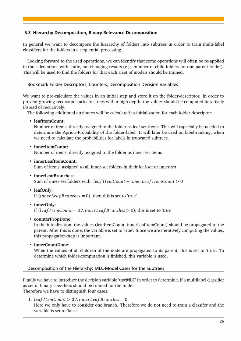
Figure 5.1: Subtree of Multilabel Classifier
As shown in Figure 5.1, we have now multiple subtrees in the hierarchy, each rooted at a trainablefolder. For each of these subtrees, we will train a set of binary classifiers as multilabel-classifier.
We can identify that the depth of these subtrees can be quite high, such that the search time can behigh and memory requirements might increase.
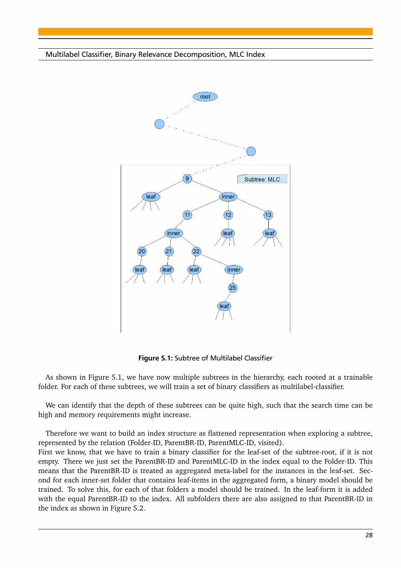
Therefore we want to build an index structure as flattened representation when exploring a subtree,represented by the relation (Folder-ID, ParentBR-ID, ParentMLC-ID, visited).First we know, that we have to train a binary classifier for the leaf-set of the subtree-root, if it is notempty. There we just set the ParentBR-ID and ParentMLC-ID in the index equal to the Folder-ID. Thismeans that the ParentBR-ID is treated as aggregated meta-label for the instances in the leaf-set. Sec-ond for each inner-set folder that contains leaf-items in the aggregated form, a binary model should betrained. To solve this, for each of that folders a model should be trained. In the leaf-form it is addedwith the equal ParentBR-ID to the index. All subfolders there are also assigned to that ParentBR-ID inthe index as shown in Figure 5.2.
28
The index is basically build through Breadth-First-Search and the resulting datasets are stored in theindex-relation as type of a ’Queue’, such that the assigned bookmarks in the subtree-collection can laterbe easily collected in a linear sequential order, reducing memory requirements.
Since in this index structure the ParentBR-ID is generally treated as aggregated meta-label, we can useit independently of which tree structure is used.
Figure 5.2: Index of the Subtree
29

5.4 Multilabel Classifier Training
Feature Subset Filtering, TF-IDF, Sparse Instance, Binary Base-Models using SVM
In general we have to identify the vocabulary that should be used in the training for each multilabelclassifier. Therefore we calculate for each token in the hierarchy the normalized-document-frequency(DF) value with respect to the training documents. For the Reuters RCV1 V2 Dataset the {train, test}-split is used as proposed with the dataset in Section 3.2 In terms of feature subset filtering [28] we willtake the tokens with the highest 5000 DF values for each classifier.
For each binary model we load all assigned instances using the index-structure and build sparsefeature-vector-representations, reduced to the training vocabulary and using the TFIDF-value for eachtoken. We can observe that this reduced vocabulary covers each instance by approx. 92%.
For the binary models we will use linear Support-Vector-Machines (SVM) [33] since it was investigated,that text classification tasks [34] [35] [36] are usually linear seperable. Therefore we do not need toapply more advanced kernel-transformation techniques. Additionally SVMs are well suited for highdimensional input spaces [29].
Generation of the binary SVM Models of the Subtree
When the index is built for a subtree rooted at a trainable folder, we can generate the SVM model files.These files should be named in the form ’MLC_<ParentMLC_ID>_BR_<ParentBR_ID>’, encoding theindex. Going through the index, all folder-bookmarks are collected and appended in their sparse feature-vector-representation to the model-file in ARFF-format1 such that the set of subtree-models can now beused to calculate predictions and determine rankings. Here the ParentBR-ID is basically representing ameta-label. Since we have to decide later, if we have to further explore a subtree rooted at the folderwith that ID, we will register a dataset with the model-file-name to a database-table, if the folder withthat ParentBR-ID has no more subfolders. This database-table will simplify the lookup on exploration.
1 http://www.cs.waikato.ac.nz/ml/weka/arff.html
30
5.5 Classifier Predictions, Bipartition, Label Ranking
When all binary SVM models down the hierarchy are built, we can calculate predictions for the models.As we initially proposed in Section 2.2 about the bookmark classification process, we want to calculate apersonalized ranking of the folders for a new query-instance, where multiple folders are assumed to bepreselected. Here we will give a short overview, how the ranking is basically built. In the next sectionwe will go more into detail, how the trained hierarchy is explored on prediction of a query-instance.
In general we have to build a ’Bipartition’ (Relevant, Irrelevant) of the set of all available bookmarkfolder descriptors. In our modelling we have two types of binary models for one folder.First, when the folder is predicted from its parent as binary model with more subfolders attached, thisis the aggregated meta-label λI D,Ag gregated , as we introduced in Section 5.1. Since we only want to rankleaf-labels, here only the subtree rooted at that folder was predicted and needs to be further resolved.Second, when the folder is predicted from its parent as binary model with no more subfolders attached,the aggregated meta-label is identical to the leaf-label λI D,Lea f and can be added to one of the sets ofthe bipartition. The probability of the prediction of the leaf-label, relative to the parent will be called’positive class prediction probability’ (PCPP).Third we have to determine a sort-order for the items inside the sets of the bipartition. Therefore downthe path from the root-node to the leaf-label, the prediction-probabilities will be multiplied, building theoverall probability for the path of each leaf-label.
In our implementation of binary models we enable the SVM option that the prediction of the positiveclass is returned as prediction probability (PCPP) related to L2-regularized logistic regression.Here we can make the assignment:
• PC PP > 0.5Here λI D is added to the set ’Relevant’
• PC PP ≤ 0.5Here λI D is added to the set ’Irrelevant’
When all labels are added to one of the two sets, the final label ranking can be determined. Thereforewe take the absolute path-probability, with that the leaf-label was predicted from the root-node of thetree. Since the leaf-label is also a meta-label with respect to the root-node, we have a child-to-parentrelation here.
The ranking is finally built over concatenation of the folder-descriptor-titles of the two ordered sets.
31
5.6 Test Instance Prediction, Exploration of the trained Hierarchy
When a new bookmark should be added to the bookmarks-tree, we first have to import the referenceddocument-sequence using our wrappers. When the tokens are indexed we can build the sparse feature-vector representation of the instance for testing using the training vocabulary. On testing of the query-instance we first create a prediction-dataset, where the root-node is assumed to be predicted with aprobability of 1.0 (100%), since the user wants to decide definitely to include the bookmark to thesubtree, rooted at the root- node. Now we can explore the trained hierarchical models to determinewhich labels should be added to one part of the bipartition.Additionally to the basic threshold 0.5 a dynamic threshold should be used in order to further expandthe predictions.
Predictions: Relevant: Basic
Here we can explore the models in a type of Breadth-First-Search.
1. Load all prediction-datasets, that were not visited and where the positive class was predicted withhigher than 0.5
2. For each prediction (parent-prediction) in list
a) Get the Parent-BR-ID
b) Set the ID as root-node of the next subtree
c) Load all models, assigned to that subtree, using the ID as Parent-MLC-ID
d) For each model in list
i. Generate a prediction of the test-instance for the model
ii. Register the prediction as dataset to the database-table
e) Set for the current parent-prediction: visited := true
When the search is finished, all predictions are visited, which predict the child from the parent withhigher than 0.5.
Predictions: Relevant: Threshold
In our experiments we want to analyse, how the results change, when the remaining unvited modelsare explored with respect to a specific threshold. Therefore we just set a threshold 0.0 ≤ t < 0.5 andrun the step, explained before for model-expansion. This will give us the possibility, that leaf-labels thatwere not found for the relevant-set before, can be added now if on a lower level in the tree a leaf-label ispositively predicted from its parent with higher than 0.5. Trivially, if the threshold is set to 0.5, this stepis finished.
Predictions: Irrelevant
When for a model the positive class was predicted with not more than the value of the threshold, thesubtree rooted at the class of this model was not further explored. For that case we define, that thissubtree was pruned for the exporation of the labels for the relevant-part of the bipartition. Here wewant to show, how these pruned subtrees can now be included to determine the second part of the bi-partition, since we want to build a label-ranking over all leaf-labels in the overall tree. First we have to
32

calculate for each pruned subtree, how much overall leaf-items are contained there. Therefore we takethe parent-BR-ID for each of these models and load the folder-descriptors. As described in Section 5.3,the total number of leaf-items in the inner-set inside the subtree, rooted at these folder is covered by thefields ’leafItemCount’ and ’innerLeafItemCount’. Next all leaf-labels of the subtree are loaded. For eachof these folder-descriptors, we take the value of the ’leafItemCount’ and ’innerLeafItemCount’- field andcalculate the apriori-probability:
• apriori(Lea f |Meta) := lea f I temCount(Lea f )lea f I temCount(Meta)+inner Lea f I temCount(Meta)
33

6 Multilabel Learning: Approaches
For each approach we consider the two phases training and prediction.
6.1 Approach 1: 1-Level, flat Tree (Binary Relevance)
Here no hierarchy is considered, such that we assume that the parent of each folder is the root node.
Phase: Training
In a flat tree, the only trainable folder is the root-node, since the other folders have no subtree. Thereforewe build the mlc index structure only for that node and generate the svm-training-models. This schemeis often called ’Binary Relevance’. For our formulation we generally treat the BR_ID as an aggregatedmeta-label to simplify the formulation for the hierarchical case. In the flat case trivially, this meta-labelis identical to the leaf-label. We can observe, that in each model-file each distinct instance of the overalltree is used, such that we have with a growing dataset a large size of the negative-set compared to thepositive-set for the binary task. This is often called ’class imbalance’.
Phase: Prediction
For a new query instance, we can just make a prediction for each model. Since the aggregated meta-labelis here identical to the leaf-label, we can add it to the bipartition depending on the prediction probability.Finally both sets are sorted by the probability and the concatenation of these two ordered sets determinesthe ranking.
6.2 Approach 2,3: Multi-Level, hierarchical Tree (HOMER)
Here we take a possible hierarchical structure into account. When for two different folders not both havethe root-node as parent, we need a more distinguished approach.
Phase: Training
In a hierarchical tree, we have multiple subtrees through the hierarchical decomposition. Thereforewe build the mlc index structure for each subtree and generate the svm-training-models. Here we areapplying an aggregated binary relevance technique on each subtree. Since each subtree covers only asubset of the instances of the overall tree, the ratio between the size of the positive-set and negative-setfor each binary model is more balanced.
Phase: Prediction
Here, for a new query instance the ranking is determined over the hierarchical exploration as explainedin Section 5.6.
34

7 Experiments
7.1 Evaluation Levels
For each test-instance a bipartition of the set of all leaf-labels is determined.For the evaluation we take different levels into account:
• L0:In the default evaluation the hierarchical relation between the labels is not considered. Thereforewe assume that all labels are on the same level.
• L1 − L5:For the hierarchical evaluation we want to take the hierarchical relations between the labels intoaccount. In the Reuters-RCV1-V2 dataset, we can observe that the labels from the root-node downthe hierarchy can be assigned to the levels 1-5.
For the evaluation measures of a specific level Li we define the base-set of labels:
• L := {λ|λ ∈ Li}
Therefore the bipartition of level 0 can be distinguished into 5 bipartitions, one for each hierarchy-level.
This is denoted by: (P0, N0) = (P1, N1), (P2, N2), (P3, N3), (P4, N4), (P5, N5)
For each hierarchy-level now the bipartition-sets are ordered by the score of each item, building theranking. Each hierarchy-level can be evaluated using the evaluation-measures.
35
7.2 Evaluation Measures
When a multi-label ranking for a test-instance x i in form of a ordered bipartition is predicted, we canevaluate the prediction using commonly known evaluation measures.
For the evaluation of the bipartition we will use the following label-based measures:
• Confusion MatrixHere we calculate for the prediction the values (tp, fp, fn, tn) of a Confusion Matrix C.tp denotes the number of labels, that were predicted positive and classified positive.fp denotes the number of labels, that were predicted positive and classified negative.fn denotes the number of labels, that were predicted negative and classified positive.tn denotes the number of labels, that were predicted negative and classified negative.Using the values of C, we calculate the measures (Precision, Recall, F1).
– Precision(C) := t ptp+ f p
– Recal l(C) := t ptp+ f n
– F1(C) := 2∗Precision(C)∗Recal l(C)Precision(C)+Recal l(C)
• Hamming LossThe Hamming Loss refers to the relevant labels that were predicted or the irrelevant labels thatwere not predicted.It is usually denoted by: Hamming Loss(x i) =
|Yi∆Zi ||L|
Here the symmetric difference Yi∆Zi denotes the misclassified labels λ ∈ L, where Yi,λ 6=Zi,λ andis given by:Yi∆Zi := {λ|(λ ∈ Yi ∧λ /∈ Zi)∨ (λ /∈ Yi ∧λ ∈ Zi)}
This denotes the label-set as result of a set-theoretic XOR-function and therefore the complementto the common intersection of Yi and Zi.
It has also been shown, that the Hamming Loss can be considered as macro-averaged classificationerror related to the confusion matrix:Hamming Loss(C) = f p+ f n
tp+ f p+ f n+tn
For the evaluation of the bipartition-ordering we will use the following label-based measures:
• Ranking LossFor the Ranking Loss first the ErrorSet for an instance x i is calculated. This is given by:ErrorSet i = {(λa,λb) : ri(λa)> ri(λb), (λa,λb) ∈ Yi × Yi}There the rank-position ri(λ) is determined as described in Section 5.2The Ranking Loss is then defined by:Ranking Loss(x i) =
1|Yi |∗|Yi |
∗ |ErrorSet i|
• Average PrecisionFor the Average Precision first the RankedAbove value for an instance x i is calculated. This is givenby:RankedAbov ei,λ = {λ′ ∈ Yi : ri(λ′)≤ ri(λ)}The Average Precision is then defined by:Av eragePrecision(x i) =
1|Yi |
∑
λ∈Yi
RankedAbov ei,λri(λ)
For the evaluation of all dataset-bipartitions we will calculate the following aggregated measures:
36
• Confusion MatrixHere we consider the Confusion Matrix C as aggregated over all cells of the instance-based matricesCi.Therefore it is denoted by: C =
∑|D|i=1 Ci
For that aggregated matrix we can calculate the Micro-Average measures (Precision, Recall, F1).These are denoted by:MicroAv gPrecision(C) := t p
tp+ f p
MicroAv gRecal l(C) := t ptp+ f n
MicroAv gF1(C) := 2∗MicroAv gPrecision(C)∗MicroAv gRecal l(C)MicroAv gPrecision(C)+MicroAv gRecal l(C)
• Hamming LossHere we calculate the (Min, Max, Avg) value over all instances in the dataset D.The average value is given by:
Hamming LossAv g(D) =∑
xi∈D Hamming Loss(xi)
|D|The (min, max) values are calculated using the instance-based matrices Ci:Hamming LossMin(D) = minxi∈D{Hamming Loss(Ci)}Hamming LossMax(D) = max xi∈D{Hamming Loss(Ci)}
For the evaluation of all bipartition-orderings in the dataset we will calculate the following aggregatedmeasures:
• Ranking LossHere we calculate the (Min, Max, Avg) value over all instances in the dataset D.The average value is given by:
Ranking LossAv g(D) =∑
xi∈D Ranking Loss(xi)
|D|The (min, max) values are calculated by:Ranking LossMin(D) = minxi∈D{Ranking Loss(x i)}Ranking LossMax(D) = max xi∈D{Ranking Loss(x i)}
• Average PrecisionHere we calculate the average value over all instances in the dataset D.The value is given by:
Av eragePrecision(D) =∑
xi∈D Av eragePrecision(xi)
|D|
37

7.3 Setup
For our experiments we will use the Reuters RCV1 V2 dataset, which we described before in Section 3.2.Out of the set of test-instances we will take the first 200.000 documents.
Therefore we define: m= |D|= 200.000
As proposed in [31] we can calculate the following statistics for our considered subset:
• Label − Cardinali t y = 1m
∑mi=1 |Yi|
Avg Number of Labels per Test-Instance
• Label − Densi t y = 1m
∑mi=1
|Yi |q
Avg Number of Labels per Test-Instance divided by q.Here q is the number of labels on the considered level.
The dataset (200.000 test-instances) is specified by the following numbers:
Level # of Labels Label-Cardinality Label-Density # of Instance-Assignments for Level-Labels0 101 3.2429 0.0321 14780911 0 0.0 0.0 02 4 1.1781 0.2945 9453343 54 1.4623 0.0271 11287844 42 1.1354 0.0270 5095465 1 1.0 1.0 23211
38

7.3.1 Configuration of the Classifier
For the binary SVM-classifiers we will use the default parameters:
• Cost: 1.0
• Bias: 1.0
• Tolerance: 0.01
• Weight of positive class: 1.0
• Weight of negative class (wneg): 1.0
In order to consider the class imbalance problem [37] [38] we will use the following parameters forthe binary SVM-classifiers in Approach 3:
• Cost: 15.0
• Weight of negative classpnratio := #instances(posi t iv e− set)/#instances(negativ e− set)wneg := pnratio+ (1− pnratio)/2
7.3.2 Configuration of the Hierarchy-Exploration
For the exploration we will use the default parameters:
• Dynamic Threshold: 0.5
For the exploration in Approach 3 we will use the parameter:
• Dynamic Threshold: 0.0
39

7.3.3 Approach 1
As explained in Section 6.1 we only have to explore binary models for one subtree, since all leaf-labelsare assumed to be assigned to the root-node. This case can be treated as single multilabel classifier.
7.3.4 Approach 2,3
As explained in Section 6.2 the hierarchical (child-to-parent) relations between the labels are taken intoaccount. Through the hierarchical decomposition we have to build one multilabel classifier for eachsubtree. Again each multilabel-classifier-subtree is represented using a set of binary models. Since thepredicted output-label of one binary model is treated as aggregated parent of a possible subtree, it canbe decided if this predicted label should be further resolved in exploration.
Approach 2.1
For the bipartition-ordering we will use the following parameters:
• Ordering of Bipartition-Positive (Z): Apriori-Probability / 2 + 0.5
• Ordering of Bipartition-Negative (Z): Apriori-Probability / 2
Approach 2.2
For the bipartition-ordering we will use the following parameters:
• Ordering of Bipartition-Positive (Z): Path-Probability / 2 + 0.5
• Ordering of Bipartition-Negative (Z): Apriori-Probability / 2
Approach 3
For the bipartition-ordering we will use the following parameters:
• Ordering of Bipartition-Positive (Z): Path-Probability / 2 + 0.5
• Ordering of Bipartition-Negative (Z): Path-Probability / 2
40

8 Evaluation
In the Reuters-RCV1-V2 dataset the root-node on level 1 has no documents assigned directly as leaf-item.Therefore it is initially assigned to the Bipartition-Negative-Set with an apriori-probability of 0.0 and theset of classified relevant labels is empty. Since we have only one label on level 5, the set of classifiedirrelevant labels for that level is empty and the ranking-loss can not be computed. Therefore we set thevalue to 0.0. For the labels of level 2 we can observe in the dataset that each instance is assigned in themulti-label associations to at least one of these labels.
41

8.1 Approach 1
• Bipartition-Measures:
Micro Average Hamming-LossTest-Instances Level Precision Recall F1 Min Max Average200000 0 0.9529 0.5208 0.6735 0.0000 0.1635 0.0157200000 1 1.0000 1.0000 1.0000 0.0000 0.0000 0.0000
2000002 0.9487 0.8224 0.8810 0.0000 1.0000 0.06543 0.9560 0.3230 0.4829 0.0000 0.1455 0.01784 0.9643 0.4096 0.5750 0.0000 0.1395 0.0090
200000 5 0.7923 0.1227 0.2125 0.0000 1.0000 0.0092
For the levels 3-5 we can observe low Recall- and F1-values as the number of negative examples inthe binary models is high related to the number of positive examples, since each binary model inthe approach contains all training-examples of the tree. This shows the class imbalance problem inthe default SVM-configuration.
• Ranking-Measures:
Ranking-Loss Ranking-PrecisionTest-Instances Level Min Max Average Average200000 0 0.0000 0.5850 0.0245 0.8556200000 1 0.0000 0.0000 0.0000 NaN
2000002 0.0000 1.0000 0.0301 0.96793 0.0000 1.0000 0.0316 0.84034 0.0000 1.0000 0.0193 0.8540
200000 5 0.0000 0.0000 0.0000 1.0000
For the evaluation of the levels 2-5 we can make the following observations:
• Level 2
– Bipartition MeasuresThe Micro-Average values are high, since each instance in the dataset is at least assigned toone of these labels. The average Hamming-Loss is high with respect to the other levels due tothe default configuration of the SVM, resulting in high FN-values in the confusion matrix.
– Ranking MeasuresThe high FN-values are resulting in a high average Ranking-Loss.
• Level 2 vs. 3
– Bipartition MeasuresThe Micro-Average values for Recall and F1 for level 3 are low. Here a large number of labelson level 3 is not predicted. In the default SVM-configuration we have a high weight on thenegative class due to the large set of negative examples.
– Ranking MeasuresThe Ranking-Loss is increasing and the AveragePrecision is decreasing, since a large set oflabels is not covered due to the class imbalance.
• Level 3 vs. 4
42

– Bipartition MeasuresThe Micro-Average values for Recall and F1 are increasing with a decreasing number of la-bels to be predicted. The values for Hamming-Loss-Max are low, since the set of labels foreach level is large and the values for (FP, FN) in the confusion matrix are low. The averageHamming-Loss is decreasing with a decreasing number of labels to be predicted.
– Ranking MeasuresThe average Ranking-Loss is decreasing and the AveragePrecision is increasing, since a lowernumber of labels needs to be predicted.
• Level 4 vs. 5
– Bipartition MeasuresThe Micro-Average values are decreasing and the average Hamming-Loss is increasing, sincethe set of labels to be predicted is smaller and the large set of negative examples in the binarymodels leads in the default configuration to wrong predictions due to the class imbalanceproblem.
43
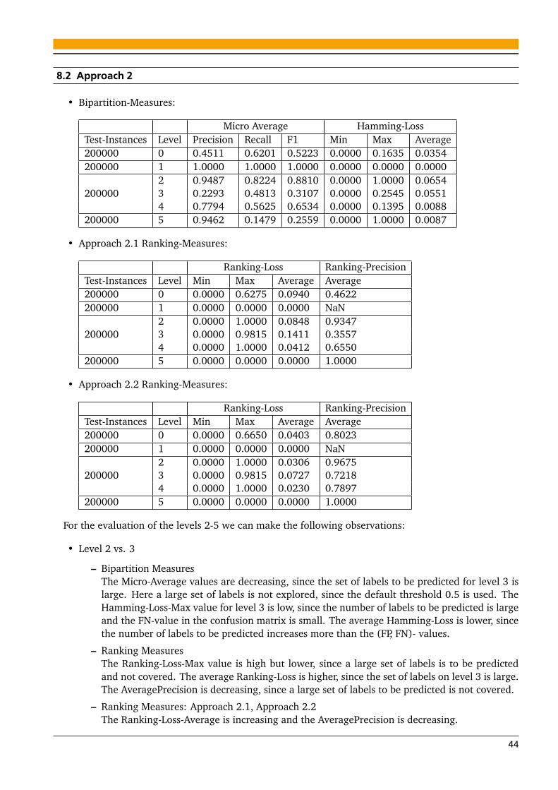
8.2 Approach 2
• Bipartition-Measures:
Micro Average Hamming-LossTest-Instances Level Precision Recall F1 Min Max Average200000 0 0.4511 0.6201 0.5223 0.0000 0.1635 0.0354200000 1 1.0000 1.0000 1.0000 0.0000 0.0000 0.0000
2000002 0.9487 0.8224 0.8810 0.0000 1.0000 0.06543 0.2293 0.4813 0.3107 0.0000 0.2545 0.05514 0.7794 0.5625 0.6534 0.0000 0.1395 0.0088
200000 5 0.9462 0.1479 0.2559 0.0000 1.0000 0.0087
• Approach 2.1 Ranking-Measures:
Ranking-Loss Ranking-PrecisionTest-Instances Level Min Max Average Average200000 0 0.0000 0.6275 0.0940 0.4622200000 1 0.0000 0.0000 0.0000 NaN
2000002 0.0000 1.0000 0.0848 0.93473 0.0000 0.9815 0.1411 0.35574 0.0000 1.0000 0.0412 0.6550
200000 5 0.0000 0.0000 0.0000 1.0000
• Approach 2.2 Ranking-Measures:
Ranking-Loss Ranking-PrecisionTest-Instances Level Min Max Average Average200000 0 0.0000 0.6650 0.0403 0.8023200000 1 0.0000 0.0000 0.0000 NaN
2000002 0.0000 1.0000 0.0306 0.96753 0.0000 0.9815 0.0727 0.72184 0.0000 1.0000 0.0230 0.7897
200000 5 0.0000 0.0000 0.0000 1.0000
For the evaluation of the levels 2-5 we can make the following observations:
• Level 2 vs. 3
– Bipartition MeasuresThe Micro-Average values are decreasing, since the set of labels to be predicted for level 3 islarge. Here a large set of labels is not explored, since the default threshold 0.5 is used. TheHamming-Loss-Max value for level 3 is low, since the number of labels to be predicted is largeand the FN-value in the confusion matrix is small. The average Hamming-Loss is lower, sincethe number of labels to be predicted increases more than the (FP, FN)- values.
– Ranking MeasuresThe Ranking-Loss-Max value is high but lower, since a large set of labels is to be predictedand not covered. The average Ranking-Loss is higher, since the set of labels on level 3 is large.The AveragePrecision is decreasing, since a large set of labels to be predicted is not covered.
– Ranking Measures: Approach 2.1, Approach 2.2The Ranking-Loss-Average is increasing and the AveragePrecision is decreasing.
44

• Level 3 vs. 4
– Bipartition MeasuresThe values for the Micro-Average measures are increasing, since the set of negative examplesfor the binary models is smaller that predict the labels of level 4. For the same reason theHamming-Loss-Max and the average Hamming-Loss are decreasing.
– Ranking MeasuresThe average Ranking-Loss is decreasing and the AveragePrecision is increasing, since the num-ber of labels to be predicted and the set of negative examples in the binary models is smaller.As the number of instance-assignments for the labels of level 4 is smaller compared to level 3,the set of instances in the decomposed binary models is smaller.
– Ranking Measures: Approach 2.1, Approach 2.2The Ranking-Loss-Average is decreasing and the AveragePrecision is increasing.
• Level 4 vs. 5
– Bipartition MeasuresThe Micro-Average-Precision is increasing, since the explored binary models make good pre-dictions. The Micro-Average Recall and F1 values are decreasing, since for a large set oftest-instances the binary models are not explored due to the static threshold.
45

8.3 Approach 3
• Bipartition-Measures:
Micro Average Hamming-LossTest-Instances Level Precision Recall F1 Min Max Average200000 0 0.4558 0.7871 0.5773 0.0000 0.2115 0.0359200000 1 1.0000 1.0000 1.0000 0.0000 0.0000 0.0000
2000002 0.9227 0.8982 0.9103 0.0000 1.0000 0.05223 0.2660 0.7143 0.3876 0.0000 0.2909 0.05824 0.7444 0.7458 0.7451 0.0000 0.1395 0.0076
200000 5 0.8653 0.6487 0.7415 0.0000 1.0000 0.0046
Since all subtrees are explored with the dynamic threshold 0.0, we can observe low FN values in theConfusion Matrix.
• Approach 3 Ranking-Measures:
Ranking-Loss Ranking-PrecisionTest-Instances Level Min Max Average Average200000 0 0.0000 0.7228 0.0236 0.8802200000 1 0.0000 0.0000 0.0000 NaN
2000002 0.0000 1.0000 0.0236 0.97513 0.0000 0.9815 0.0403 0.84144 0.0000 1.0000 0.0129 0.8726
200000 5 0.0000 0.0000 0.0000 1.0000
Here more labels are moved from bipartition-negative to bipartition-positive. Additionally the labelsin bipartition-negative are ordered by the path-probability, leading to an overall higher average Ranking-Precision.
For the evaluation of the levels 2-5 we can make the following observations:
• Level 2 vs. 3
– Bipartition MeasuresThe Micro-Average values are decreasing, since the set of labels to be predicted for level 3is large. The Hamming-Loss-Max value for level 3 is low, since the number of labels to bepredicted is large and the FN-value in the confusion matrix is small.
– Ranking MeasuresThe average Ranking-Loss is increasing and the AveragePrecision is decreasing, since the setof labels on level 3 is large.
• Level 3 vs. 4
– Bipartition MeasuresComparable high number of labels to be predicted on both levels Labels to be predicted loweron level 4. The values for the Micro-Average measures are increasing, since the set of negativeexamples for the binary models is smaller that predict the labels of level 4. For the same reasonthe Hamming-Loss-Max and the average Hamming-Loss are decreasing.
46

– Ranking MeasuresThe average Ranking-Loss is decreasing and the AveragePrecision is increasing, since the num-ber of labels to be predicted and the set of negative examples in the binary models is smaller.As the number of instance-assignments for the labels of level 4 is smaller compared to level 3,the set of instances in the decomposed binary models is smaller.
• Level 4 vs. 5
– Bipartition MeasuresThe Micro-Average-Precision is increasing, since the explored binary models make good pre-dictions.
47

8.4 Approach 1 vs. 2
• Bipartition Measures:
– Level 3,4,5: Here we can observe an increasing Micro Average Recall value
– Level 3,4,5: Here we can observe an increasing Hamming-Loss Average value
– Level 4,5: Here we can observe an increasing Micro Average F1 value
– Level 5: Here we can observe an increasing Micro Average Precision value
At the levels 4,5 in the hierarchical modelling the negative-set of instances is small. Therefore theweight between the positive class and negative class is relatively balanced.
• Ranking Measures:
– Level 2 vs 3: Here the Ranking-Loss Average is increasing and the Ranking-Precision Averageis decreasing
– Level 3 vs 4: Here the Ranking-Loss Average is decreasing and the Ranking-Precision Averageis increasing
8.5 Approach 2 vs. 3
• Bipartition Measures:
– Level 0,2,3,4,5: Here we can observe an increasing Micro Average Recall and F1 values
– Level 4,5: Here we can observe an decreasing Hamming-Loss Average value
At the levels 4,5 in the hierarchical modelling the negative-set of instances is small. Therefore theweight between the positive class and negative class is relatively balanced.
Since all subtrees of the hierarchical dataset are explored we can observe higher tp and fp valuesin the confusion-matrices for the levels 0,2,3,4.
• Ranking Measures:
– Level 0,2,3,4,5: Here the Ranking-Loss Average is decreasing
– Level 0,2,3,4: Here Ranking-Precision Average is increasing
Here both parts of the bipartition are ordered by the path-probability.
48

9 Conclusions, Further Work
In this thesis we could show the evaluation of two different decomposition techniques for the multi- labelhierarchical dataset Reuters-RCV1-V2.Therefore we calculated bipartition-measures and ranking-measures for different levels of the hierarchy.For the hierarchical dataset-modelling we could show an improvement for the lower levels of the hierar-chy, since there less instances are considered in the negative-set of the binary models. We conclude thatthe class imbalance there is relatively low.Using the dynamic threshold in the exploration, a higher cost value and a lower weight of the negativeclass for the binary models we could show an improvement in the rankings.
Basically we set each subtree-MLC (set of binary classifiers) to the default SVM-configuration for eachhierarchy-level. Looking forward to further developments, it can be considered to set different configu-rations for the levels / subtree-MLCs.
For the further work, user-generated content in terms of text-summaries and the reorganization of thetree-structure can be taken into account. This is partially adressed as gradual forgetting.
49

Acknowledgements
We want to thank Frédéric R. Bürthel (MarketDialog GmbH) for his support in Metadata Modelling andDigital Library Tools.
50

List of Figures
5.1 Subtree of Multilabel Classifier . . . . . . . . . . . . . . . . . . . . . . . . . . . . . . . . . . . . . 285.2 Index of the Subtree . . . . . . . . . . . . . . . . . . . . . . . . . . . . . . . . . . . . . . . . . . . 29
51
Bibliography
[1] D. Barreau and B. Nardi, “Finding and reminding: File organization from the desktop,” ACM SIGCHIBulletin, vol. Vol. 27 (3), July 1995.
[2] S. Dumais, E. Cutrell, J. J. Cadiz, G. Jancke, R. Sarin, and D. C. Robbins, “Stuff i’ve seen: asystem for personal information retrieval and re-use,” in SIGIR ’03 Proceedings of the 26th annualinternational ACM SIGIR conference on Research and development in informaion retrieval, vol. 26,pp. 72 – 79, ACM New York, NY, USA, 2003.
[3] V. Bush, “As we may think,” Atlantic Monthly, vol. 176, pp. 101 – 108, 1945.
[4] D. Abrams, R. Baecker, and M. Chignell, “Information archiving with bookmarks: Personal webspace construction and organization,” In ACM SIGCHI ’98, pp. 41–48, 1998.
[5] M. J. Hofmann, L. Kuchinke, C. Biemann, S. Tamm, and A. M. Jacobs, “Remembering words incontext as predicted by an associative read-out model,” Frontiers in psychology, vol. 2, 2011.
[6] J. Grainger and A. M. Jacobs, “Orthographic processing in visual word recognition: a multipleread-out model.,” Psychological review, vol. 103, no. 3, p. 518, 1996.
[7] M. S. Seidenberg and J. L. McClelland, “A distributed, developmental model of word recognitionand naming,” Psychological review, vol. 96, p. 523, 1989.
[8] M. E. Casey and L. C. Savastinuk, “Library 2.0: Service for the next-generation library,” LibraryJournal, 2006.
[9] J. M. Maness, “Library 2.0 theory: Web 2.0 and its implications for libraries,” Webology, vol. Vol. 3(2), June, 2006.
[10] A. Foster and N. Ford, “Serendipity and information seeking: an empirical study,” Journal of Docu-mentation, vol. Vol. 59 (3), pp. 321 – 340, 2003.
[11] A. Spink, M. Park, B. J. Jansen, and J. Pedersen, “Multitasking during web search sessions,” Inf.Process. Manage., vol. 42, pp. 264–275, Jan. 2006.
[12] S. Whittaker and C. Sidner, “Email overload: exploring personal information management ofemail,” in Proceedings of the SIGCHI conference on Human factors in computing systems: commonground, (Vancouver, British Columbia, Canada), ACM, 1996.
[13] C. Speier, J. S. Valacich, and I. Vessey, “The influence of task interruption on individual decisionmaking: An information overload perspective,” Decision Sciences, vol. Vol. 30, pp. 337 – 360, 1999.
[14] O. Serrat, “Showcasing knowledge,” Washington, DC: Asian Development Bank, 2010.
[15] P. Morville and L. Rosenfeld, Information Architecture for the world wide web: designing large-scaleweb sites. O’Reilly, 2006.
[16] M. Ehrig and A. Maedche, “Ontology-focused crawling of web documents,” in SAC ’03 Proceedingsof the 2003 ACM symposium on Applied computing, pp. 1174–1178, 2003.
[17] J. Huang and R. W. White, “Parallel browsing behavior on the web,” in Proceedings of the 21st ACMconference on Hypertext and hypermedia, HT ’10, (New York, NY, USA), pp. 13–18, ACM, 2010.
52
[18] R. D. García, Unterstützung des Ressourcen-Basierten Lernens in Online Communities - AutomatischeErstellung von Grosstaxonomien in verschiedenen Sprachen. PhD thesis, Fachbereich Elektrotechnikund Informationstechnik der Technischen Universität Darmstadt, 2013.
[19] D. E. Rumelhart and J. L. McClelland, “An interactive activation model of context effects in letterperception: Ii. the contextual enhancement effect and some tests and extensions of the model.,”Psychological Review, vol. 89(1), pp. 60 – 94, 1982.
[20] M. Coltheart, K. Rastle, C. Perry, R. Langdon, and J. Ziegler, “Drc: a dual route cascaded model ofvisual word recognition and reading aloud.,” Psychological review, vol. 108, no. 1, p. 204, 2001.
[21] M. Lansdale, “The psychology of personal information management,” Applied Ergonomics, pp. 55 –66, 1988.
[22] R. Mander, G. Salomon, and Y. Y. Wong, “A "pile" metaphor for supporting casual organizationof information,” in CHI ’92 Proceedings of the SIGCHI Conference on Human Factors in ComputingSystems, pp. 627 – 634, ACM, 1992.
[23] I. Katakis, G. Tsoumakas, and I. P. Vlahavas, “Multilabel text classification for automated tag sug-gestion,” in Proceedings of the ECML/PKDD-08 Workshop on Discovery Challenge, 2008.
[24] E. S. Xioufis, M. Spiliopoulou, G. Tsoumakas, and I. & Vlahavas, “Dealing with concept drift andclass imbalance in multi-label stream classification,” in Proceedings of the Twenty-Second interna-tional joint conference on Artificial Intelligence-Volume, vol. Vol. 2, pp. 1583 – 1588, AAAI Press,2011.
[25] E. L. Cohen, “Online journalism as market-driven journalism,” Journal of Broadcasting & ElectronicMedia, vol. Vol. 46 (4), pp. 532 – 548, 2002.
[26] A. Bruns, Gatewatching: Collaborative online news production, vol. Vol. 26. Peter Lang Pub Incorpo-rated, 2005.
[27] D. D. Lewis, Y. Yang, T. Rose, and F. Li, “Rcv1: A new benchmark collection for text categorizationresearch,” Journal of Machine Learning Research, vol. Vol. 5, pp. 361 – 397, 2004.
[28] R. Kohavi and G. H. John, “Wrappers for feature subset selection,” Artificial Intelligence, vol. Vol.97 (1-2), pp. 273 – 324, December 1997.
[29] T. Joachims, “Text categorization with suport vector machines: Learning with many relevant fea-tures,” in ECML ’98 Proceedings of the 10th European Conference on Machine Learning, pp. 137 –142, Springer-Verlag London, UK, 1998.
[30] K. Brinker, J. Fürnkranz, and E. Hüllermeier, “A unified model for multilabel classification and rank-ing,” in IN PROCEEDINGS OF THE 17TH EUROPEAN CONFERENCE ON ARTIFICIAL INTELLIGENCE,pp. 489–493, 2006.
[31] G. Tsoumakas, I. Katakis, and I. P. Vlahavas, “Mining multi-label data,” in In Data Mining andKnowledge Discovery Handbook, pp. 667–685, 2010.
[32] G. Tsoumakas, I. Katakis, and I. P. Vlahavas, “Effective and efficient multilabel classification indomains with large number of labels,” in ECML/PKDD 2008 Workshop on Mining MultidimensionalData, 2008.
[33] R.-E. Fan, K.-W. Chang, C.-J. Hsieh, X.-R. Wang, and C.-J. Lin, “Liblinear a library for large linearclassification,” The Journal of Machine Learning Research, vol. Vol. 9, pp. 1871 – 1874, 2008.
53

[34] E. Leopold and J. Kindermann, “Text categorization with support vector machines. how to representtexts in input space?,” Machine Learning, vol. Vol. 46 Issue 1-3, pp. 423 – 444, 2002.
[35] L. Cai and T. Hofmann, “Hierarchical document categorization with support vector machines,” inCIKM ’04 Proceedings of the thirteenth ACM international conference on Information and knowledgemanagement, pp. 78 – 87, ACM New York, NY, USA, 2004.
[36] M. Lan, C.-L. Tan, H.-B. Low, and S.-Y. Sung, “A comprehensive comparative study on term weight-ing schemes for text categorization with support vector machines,” in WWW ’05 Special interesttracks and posters of the 14th international conference on World Wide Web, pp. 1032 – 1033, ACMNew York, NY, USA, 2005.
[37] U. Brefeld, P. Geibel, and F. Wysotzki, “Support vector machines with example dependent costs,” inMachine Learning: ECML 2003, pp. 23 – 34, Springer, 2003.
[38] C. Drummond and R. C. Holte, “Severe class imbalance: Why better algorithms aren’t the answer,”in Machine Learning: ECML 2005, pp. 539 – 546, Springer, 2005.
54