multilevel analysis - princeton university

PU/DSS/OTR

Multilevel Analysis(ver. 1.0)

Oscar Torres-ReynaData [email protected]

http://dss.princeton.edu/training/

PU/DSS/OTR

2

Use multilevel model whenever your data is grouped (or nested) in more than one category (for example, states, countries, etc).

Multilevel models allow:

• Study effects that vary by entity (or groups) • Estimate group level averages

Some advantages:

• Regular regression ignores the average variation between entities.• Individual regression may face sample problems and lack of

generalization

Motivation

PU/DSS/OTR

3

-40

-20

020

40y

0 20 40 60school

Score y_mean

use http://dss.princeton.edu/training/schools.dtabysort school: egen y_mean=mean(y)twoway scatter y school, msize(tiny) || connected y_mean school, connect(L) clwidth(thick) clcolor(black) mcolor(black) msymbol(none) || , ytitle(y)

Variation between entities

PU/DSS/OTR

4

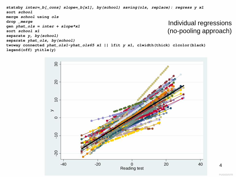
statsby inter=_b[_cons] slope=_b[x1], by(school) saving(ols, replace): regress y x1sort schoolmerge school using olsdrop _mergegen yhat_ols = inter + slope*x1sort school x1separate y, by(school)separate yhat_ols, by(school)twoway connected yhat_ols1-yhat_ols65 x1 || lfit y x1, clwidth(thick) clcolor(black) legend(off) ytitle(y)

-20

-10

010

2030

y

-40 -20 0 20 40Reading test

Individual regressions (no-pooling approach)

PU/DSS/OTR

LR test vs. linear regression: chibar2(01) = 498.72 Prob >= chibar2 = 0.0000 sd(Residual) 9.207357 .1030214 9.007636 9.411505 sd(_cons) 4.106553 .3999163 3.392995 4.970174school: Identity Random-effects Parameters Estimate Std. Err. [95% Conf. Interval]

_cons -.1317104 .536272 -0.25 0.806 -1.182784 .9193634 y Coef. Std. Err. z P>|z| [95% Conf. Interval]

Log likelihood = -14851.502 Prob > chi2 = . Wald chi2(0) = .

max = 198 avg = 62.4 Obs per group: min = 2

Group variable: school Number of groups = 65Mixed-effects ML regression Number of obs = 4059

. xtmixed y || school: , mle nolog

5

Standard deviation at the school level (level 2)

Standard deviation at the individual level (level 2)

Mean of state level intercepts

17.021.911.4

11.4)()(_

)(_)_()_(

)_(_ 22

2

22

2

22

2

=+

=+

=+

=residualsdconssd

conssdesigmausigma

usigmancorrelatioIntraclass

“An intraclass correlation tells you about the correlation of the observations (cases) within a cluster” (http://www.ats.ucla.edu/stat/Stata/Library/cpsu.htm)

If the interclass correlation (IC) approaches 0 then the grouping by counties (or entities) are of no use (you may as well run asimple regression). If the IC approaches 1 then there is no variance to explain at the individual level, everybody is the same.

Varying-intercept model (null) iijiy εα += ][

Ho: Random-effects = 0

http://www.ats.ucla.edu/stat/Stata/Library/cpsu.htm�

otorres

Typewritten Text

NOTE: Stata 13, the command changed to "mixed"

PU/DSS/OTR

6




14.052.703.3

03.3)()(_

)(_)_()_(

)_(_ 22

2

22

2

22

2

=+

=+

=+

=residualsdconssd

conssdesigmausigma


“An intraclass correlation tells you about the correlation of the observations (cases) within a cluster” (http://www.ats.ucla.edu/stat/Stata/Library/cpsu.htm)

If the interclass correlation (IC) approaches 0 then the grouping by counties (or entities) are of no use (you may as well run asimple regression). If the IC approaches 1 then there is no variance to explain at the individual level, everybody is the same.

Varying-intercept model (one level-1 predictor)

LR test vs. linear regression: chibar2(01) = 403.27 Prob >= chibar2 = 0.0000 sd(Residual) 7.521481 .0841759 7.358295 7.688285 sd(_cons) 3.035271 .3052516 2.492262 3.69659school: Identity Random-effects Parameters Estimate Std. Err. [95% Conf. Interval]

_cons .0238706 .4002258 0.06 0.952 -.7605576 .8082987 x1 .5633697 .0124654 45.19 0.000 .5389381 .5878014 y Coef. Std. Err. z P>|z| [95% Conf. Interval]

Log likelihood = -14024.799 Prob > chi2 = 0.0000 Wald chi2(1) = 2042.57



. xtmixed y x1 || school: , mle nolog

iiiji xy εβα ++= ][


http://www.ats.ucla.edu/stat/Stata/Library/cpsu.htm�

PU/DSS/OTR

7




14.044.701.312.0

01.312.0)()1()(_

)1()(_)_()_(

)_(_ 222

22

22

2

22

2

=++

+=

+++

=+

=residualsdxsdconssdxsdconssd

esigmausigmausigmancorrelatioIntraclass

Varying-intercept, varying-coefficient model

Note: LR test is conservative and provided only for reference.

LR test vs. linear regression: chi2(3) = 443.64 Prob > chi2 = 0.0000 sd(Residual) 7.440788 .0839482 7.278059 7.607157 corr(x1,_cons) .4975474 .1487416 .1572843 .7322131 sd(_cons) 3.007436 .3044138 2.466252 3.667375 sd(x1) .1205631 .0189827 .0885508 .1641483school: Unstructured Random-effects Parameters Estimate Std. Err. [95% Conf. Interval]

_cons -.1150841 .3978336 -0.29 0.772 -.8948236 .6646554 x1 .5567291 .0199367 27.92 0.000 .5176539 .5958043 y Coef. Std. Err. z P>|z| [95% Conf. Interval]




. xtmixed y x1 || school: x1, mle nolog covariance(unstructure)

iiijiji xy εβα ++= ][][


PU/DSS/OTR

8




Varying-slope model

LR test vs. linear regression: chibar2(01) = 0.00 Prob >= chibar2 = 1.0000 sd(Residual) 8.052417 .089372 7.879142 8.229502 sd(R.x1) .0003388 .1806391 0 ._all: Identity Random-effects Parameters Estimate Std. Err. [95% Conf. Interval]




Group variable: _all Number of groups = 1Mixed-effects ML regression Number of obs = 4059

. xtmixed y x1 || _all: R.x1, mle nolog

iiiji xy εβα ++= ][

PU/DSS/OTR

9

Postestimation

PU/DSS/OTR

10

Comparing models using likelihood-ration test

Use the likelihood-ratio test (lrtest) to compare models fitted by maximum likelihood. This test compares the “log likelihood” (shown in the output) of two models and tests whether they are significantly different.

/*Fitting random intercepts and storing results*/quietly xtmixed y x1 || school: , mle nologestimates store ri

/*Fitting random coefficients and storing results*/quietly xtmixed y x1 || school: x1, mle nolog covariance(unstructure)estimates store rc

/*Running the likelihood-ratio test to compare*/lrtest ri rc

Note: LR test is conservative

(Assumption: ri nested in rc) Prob > chi2 = 0.0000Likelihood-ratio test LR chi2(2) = 40.37

. lrtest ri rc

The null hypothesis is that there is no significant difference between the two models. If Prob>chi2<0.05, then you may reject the null and conclude that there is a statistically significant difference between the models. In the example above we reject the null and conclude that the random coefficients model provides a better fit (it has the lowest log likelihood)

PU/DSS/OTR

11




14.0365.55045.9014.0

045.9014.0)var()1var()var(_

)1var()var(_)_()_(

)_(_ 2 =++

+=

+++

=+

=residualxcons

xconsesigmausigma


Varying-intercept, varying-coefficient model: postestimation


LR test vs. linear regression: chi2(3) = 443.64 Prob > chi2 = 0.0000 var(Residual) 55.36533 1.249282 52.97014 57.86883 cov(x1,_cons) .1804036 .0691515 .0448692 .315938 var(_cons) 9.04467 1.83101 6.082398 13.44964 var(x1) .0145355 .0045772 .0078412 .0269446school: Unstructured Random-effects Parameters Estimate Std. Err. [95% Conf. Interval]





. xtmixed y x1 || school: x1, mle nolog covariance(unstructure) variance

PU/DSS/OTR

12

Postestimation: variance-covariance matrix

. xtmixed y x1 || school: x1, mle nolog covariance(unstructure) variance


LR test vs. linear regression: chi2(3) = 443.64 Prob > chi2 = 0.0000 var(Residual) 55.36533 1.249282 52.97014 57.86883 cov(x1,_cons) .1804036 .0691515 .0448692 .315938 var(_cons) 9.04467 1.83101 6.082398 13.44964 var(x1) .0145355 .0045772 .0078412 .0269446school: Unstructured Random-effects Parameters Estimate Std. Err. [95% Conf. Interval]

_cons .4975474 1 x1 1 x1 _cons

Random-effects correlation matrix for level school

. estat recovariance, correlation

_cons .1804036 9.04467 x1 .0145355 x1 _cons

Random-effects covariance matrix for level school

. estat recovariance

Variance-covariance matrix

The correlation between the intercept and x1 shows a close relationship between the average of y and x1.

PU/DSS/OTR

13

Postestimation: estimating random effects (group-level errors)

To estimate the random effects u, use the command predict with the option reffects, this will give you the best linear unbiased predictions (BLUPs) of the random effects which basically show the amount of variation for both the intercept and the estimated beta coefficient(s). After running xtmixed, type

predict u*, reffects

Two new variables are created

u1 “BLUP r.e. for school: x1” ------- /* uβ */u2 “BLUP r.e. for school: _cons” --- /* uα */

iiijiji xy εβα ++= ][][ iiijiji ijiuuxy εβα βα ++++=

][][][

Fixed-effects Random-effects

PU/DSS/OTR

14

Postestimation: estimating random effects (group-level errors)

156.012.0 xyi +−= βα uuxyi +++−= 156.012.0

Fixed-effects Random-effectsTo explore some results type:

bysort school: generate groups=(_n==1) /*_n==1 selects the firstcase of each group */

list school u2 u1 if school<=10 & groups

599. 10 -3.139076 -.1360763 565. 9 -1.767982 -.0886194 463. 8 -.121886 .0068855 375. 7 3.640942 -.1488697 295. 6 5.183809 .0586242 260. 5 2.462805 .0720576 181. 4 .3502505 .1271821 129. 3 4.79768 .0808666 74. 2 4.702129 .1647261 1. 1 3.749336 .1249755 school u2 u1

. list school u2 u1 if school<=10 & groups

Here u2 and u1 are the group level errors for the intercept and the slope respectively. For the first school the equation would be:

168.063.31)12.056.0()75.312.0(12.075.3156.012.01 xxxy +=+++−=+++−=

PU/DSS/OTR

15

Postestimation: estimating intercept/slope

To estimate intercepts and slopes per school type :

gen intercept = _b[_cons] + u2gen slope = _b[x1] + u1list school intercept slope if school<=10 & groups

Compare the coefficients for school 1 above

599. 10 -3.254161 .4206528 565. 9 -1.883067 .4681097 463. 8 -.2369701 .5636145 375. 7 3.525858 .4078594 295. 6 5.068725 .6153533 260. 5 2.347721 .6287867 181. 4 .2351664 .6839111 129. 3 4.682596 .6375957 74. 2 4.587045 .7214552 1. 1 3.634251 .6817045 school intercept slope

. list school intercept slope if school<=10 & groups

168.063.31)12.056.0()75.312.0(12.075.3156.012.01 xxxy +=+++−=+++−=

PU/DSS/OTR

16

Postestimation: fitting values

Using intercept and slope you can estimate yhat, type

gen yhat= intercept + (slope*x1)

Or, after xtmixed type:

predict yhat_fit, fitted

list school yhat yhat_fit if school<=10 & groups

599. 10 -9.341847 -9.341847 565. 9 -15.62209 -15.62209 463. 8 -13.98353 -13.98353 375. 7 -6.084939 -6.084939 295. 6 -3.836668 -3.836667 260. 5 -5.193317 -5.193318 181. 4 -15.88052 -15.88052 129. 3 -7.179871 -7.179871 74. 2 -15.3951 -15.3951 1. 1 -12.42943 -12.42943 school yhat yhat_fit

. list school yhat yhat_fit if school<=10 & groups

PU/DSS/OTR

17

Postestimation: fittied values (graph)You can plot individual regressions, type

twoway connected yhat_fit x1 if school<=10, connect(L)

-20

-10

010

20Fi

tted

valu

es: x

b +

Zu

-40 -20 0 20 40Reading test

PU/DSS/OTR

18

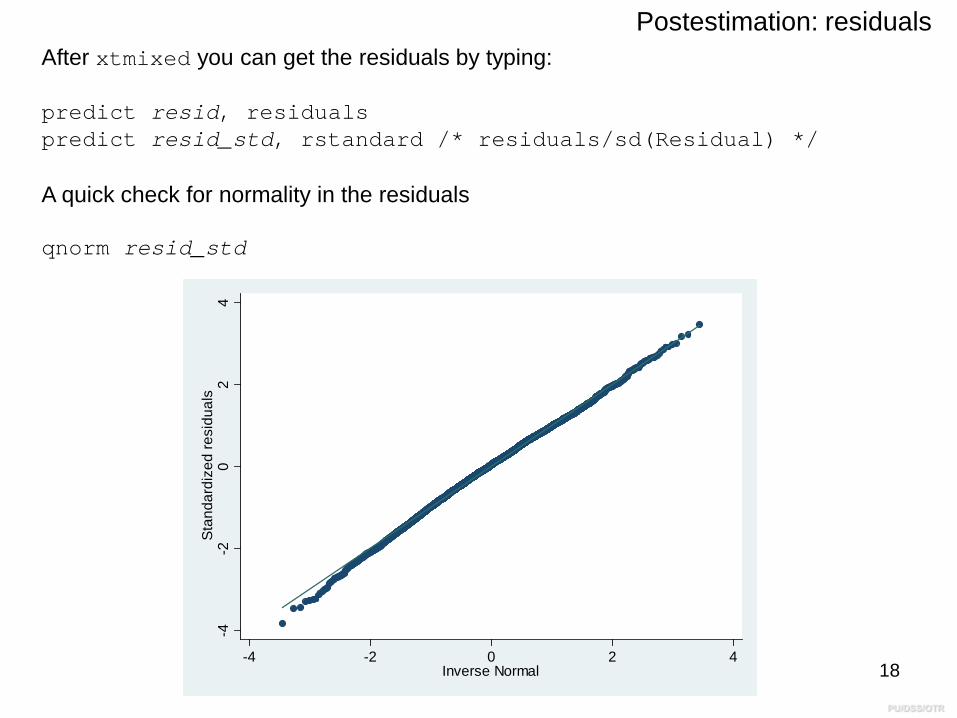
Postestimation: residuals After xtmixed you can get the residuals by typing:

predict resid, residualspredict resid_std, rstandard /* residuals/sd(Residual) */

A quick check for normality in the residuals

qnorm resid_std-4

-20

24

Stan

dard

ized

resi

dual

s

-4 -2 0 2 4Inverse Normal

PU/DSS/OTR

19

Useful links / Recommended books / References• DSS Online Training Section http://dss.princeton.edu/training/• UCLA Resources http://www.ats.ucla.edu/stat/• Princeton DSS Libguides http://libguides.princeton.edu/dss

Books/References

• “Beyond “Fixed Versus Random Effects”: A framework for improving substantive and statistical analysis of panel, time-series cross-sectional, and multilevel data” / Brandom Bartels http://polmeth.wustl.edu/retrieve.php?id=838

• “Robust Standard Errors for Panel Regressions with Cross-Sectional Dependence” / Daniel Hoechle, http://fmwww.bc.edu/repec/bocode/x/xtscc_paper.pdf

• An Introduction to Modern Econometrics Using Stata/ Christopher F. Baum, Stata Press, 2006.• Data analysis using regression and multilevel/hierarchical models / Andrew Gelman, Jennifer Hill.

Cambridge ; New York : Cambridge University Press, 2007. • Data Analysis Using Stata/ Ulrich Kohler, Frauke Kreuter, 2nd ed., Stata Press, 2009.• Designing Social Inquiry: Scientific Inference in Qualitative Research / Gary King, Robert O.

Keohane, Sidney Verba, Princeton University Press, 1994.• Econometric analysis / William H. Greene. 6th ed., Upper Saddle River, N.J. : Prentice Hall, 2008.• Introduction to econometrics / James H. Stock, Mark W. Watson. 2nd ed., Boston: Pearson Addison

Wesley, 2007.• Statistical Analysis: an interdisciplinary introduction to univariate & multivariate methods / Sam

Kachigan, New York : Radius Press, c1986• Statistics with Stata (updated for version 9) / Lawrence Hamilton, Thomson Books/Cole, 2006• Unifying Political Methodology: The Likelihood Theory of Statistical Inference / Gary King, Cambridge

University Press, 1989

http://dss.princeton.edu/training/�

http://www.ats.ucla.edu/stat/�

http://libguides.princeton.edu/dss�

http://polmeth.wustl.edu/retrieve.php?id=838�

http://fmwww.bc.edu/repec/bocode/x/xtscc_paper.pdf�

multilevel analysis - princeton university

Documents