multilevel and algebraic multigrid methods for the higher...
TRANSCRIPT

Multilevel and Algebraic Multigrid Methods
for the Higher Order Finite Element Analysis of
Time Harmonic Maxwell’s Equations
Ali Aghabarati
Department of Electrical & Computer Engineering
McGill University
Montreal, Canada
October 2013
A thesis submitted to McGill University in partial fulfillment of the requirements for
the degree of Doctor of Philosophy.
© Ali Aghabarati, 2013

i
Dedicated to My Family

ii
Abstract The Finite Element Method (FEM) applied to wave scattering and quasi-static
vector field problems in the frequency domain leads to sparse, complex-symmetric,
linear systems of equations. For large problems with complicated geometries, most of
the computer time and memory used by FEM goes to solving the matrix equation.
Krylov subspace methods are widely used iterative methods for solving large sparse
systems. They depend heavily on preconditioning to accelerate convergence.
However, application of conventional preconditioners to the “curl-curl” operator
which arises in vector electromagnetics does not result in a satisfactory performance
and specialized preconditioning techniques are required.
This thesis presents effective Multilevel and Algebraic Multigrid (AMG)
preconditioning techniques for p-adaptive FEM analysis. In p-adaption, finite
elements of different polynomial orders are present in the mesh and the system matrix
can be structured into blocks corresponding to the orders of the basis functions. The
new preconditioners are based on a p-type multilevel Schwarz (pMUS) approximate
inversion of the block structured system. A V-cycle multilevel correction starts by
applying Gauss-Seidel to the highest block level, then the next level down, and so on.
On the other side of the V, Gauss-Seidel iterations are applied in the reverse order. At
the bottom of the cycle is the lowest order system, which is usually solved exactly
with a direct solver. The proposed alternative is to use Auxiliary Space
Preconditioning (ASP) at the lowest level and continue the V-cycle downwards, first
into a set of auxiliary, node-based spaces, then through a series of progressively
smaller matrices generated by an Algebraic Multigrid (AMG). The algebraic
coarsening approach is especially useful for problems with fine geometric details,
requiring a very large mesh in which the bulk of the elements remain at low order.
In addition, for wave problems, a “shifted Laplace” technique is applied, in which
part of the ASP/AMG algorithm uses a perturbed, complex frequency. A significant
convergence acceleration is achieved. The performance of Krylov algorithms is
further enhanced during p-adaption by incorporation of a deflation technique. This
projects out from the preconditioned system the eigenvectors corresponding to the
smallest eigenvalues. The construction of the deflation subspace is based on efficient
estimation of the eigenvectors from information obtained when solving the first
problem in a p-adaptive sequence.

iii
Extensive numerical experiments have been performed and results are presented
for both wave and quasi-static problems. The test cases considered are complicated to
solve and the numerical results show the robustness and efficiency of the new
preconditioners. Deflated Krylov methods preconditioned with the current
Multilevel/ASP/AMG approach are always considerably faster than the reference
methods and speedups of up to 10 are achieved for some test problems.

iv
Résumé
La méthode des éléments finis (FEM) appliquée à la dispersion des ondes et aux
problèmes de champ de vecteurs quasi-statique dans le domaine fréquentiel mène à
des systèmes d'équations linéaires rares, symétriques-complexes. Pour de grands
problèmes ayant des géométries complexes, la plupart du temps et de la mémoire
d'ordinateur utilisé par FEM va à la résolution de l'équation de la matrice. Les
méthodes itératives de Krylov sont celles largement utilisées dans la résolution de
grands systèmes creux. Elles dépendent fortement des préconditionnement qui
accélèrent la convergence. Toutefois, l'application de préconditionnements
conventionnels à l'opérateur "rot-rot" qui surgit en électromagnétisme vectoriel
n'aboutit pas à des résultats satisfaisants et des techniques de préconditionnement
spécialisés sont exigées.
Cette thèse présente des techniques de préconditionnement efficaces multiniveau
et multigrilles algébrique (AMG) pour l'analyse p-adaptative FEM. Dans la p-
adaptation, des éléments finis de différents ordres polynomiaux sont présents dans le
maillage et la matrice du système peut être structurée en blocs correspondant aux
ordres des fonctions de base. Les nouveaux préconditionneurs sont basés sur un type
d'inversion approximative à multiniveau p Schwarz (pMUS) du système structuré de
bloc. Une correction à niveaux multiples en cycle V débute par l'application de Gauss-
Seidel au niveau du bloc le plus élevé, suivi par le niveau inférieur, et ainsi de suite.
De l'autre côté du V, des itérations de Gauss-Seidel sont appliquées en ordre inverse.
Au bas du cycle se trouve le système d'ordre le plus bas, qui est habituellement résolu
exactement avec un solveur direct. L'alternative proposée est d'utiliser l'espace
auxiliaire de préconditionnement (ASP) au niveau le plus bas et de poursuivre le cycle
en V vers le bas, d'abord en un ensemble d'auxiliaires, basé sur les espacements de
nœuds, à travers une série de plus en plus petites de matrices générées par un
multigrille algébrique (AMG). L'approche de grossissement algébrique est
particulièrement utile aux problèmes ayant de fins détails géométriques, nécessitant
une très grande maille dans laquelle la majeure partie des éléments restent à un niveau
plus bas.
En outre, pour des problèmes d'onde, la technique "décalé Laplace" est appliquée,
dans laquelle une partie de l'algorithme ASP/AMG utilise une fréquence complexe

v
perturbée. Une accélération de la convergence significative est atteinte. La
performance des algorithmes de Krylov est davantage renforcée au cours du p-
adaptation par l'incorporation d'une technique de déflation. Cette saillie fait dépasser
hors du système préconditionné, les vecteurs propres correspondants aux plus petites
valeurs propres. La construction du sous-espace de déflation est basée sur une
estimation efficace des vecteurs propres à partir d'informations obtenues lors de la
résolution du premier problème dans une séquence p-adaptatif.
Des expériences numériques approfondies ont été effectuées et les résultats sont
présentés à la fois aux problèmes d'onde et quasi-statiques. Les cas de test sont
considérés comme compliqués à résoudre et les résultats numériques montrent la
robustesse et l'efficacité des nouveaux préconditionnements. Les méthodes de Krylov
de déflation préconditionnés par l'approche multiniveaux/ASP/AMG actuelle sont
toujours considérablement plus rapides que les méthodes de référence et des
accélérations allant jusqu'à 10 sont atteintes pour certains problèmes de test.

vi
Acknowledgments
First and foremost, I need to thank my supervisor Prof. Jon P Webb, for his
continuous guidance and support throughout my program. His wide knowledge and
generous insight gave me significant help during this research work. His pro-active
and well-organized attitude in scientific research also set a great example for me.
Without his help the completion of this thesis would not have been possible and I wish
to express my sincere gratitude.
I am also grateful to my Ph.D. committee members: Prof. Dennis Giannacopoulos
and Prof. Roni Khazaka, for their valuable advice, suggestions and the time they
devoted to my research work. I also wish to extend my thanks to Prof. Romanus
Dyczij-Edlinger, Prof. David Lowther, Prof. Hani Mitri and Prof. Richard Rose for
accepting to review this thesis as members of the jury. I am confident that I will
benefit a great deal from the comments and suggestions.
During my study at McGill, I had the privilege of working closely with many
friends. My sincere appreciation goes to Dr. Hussein Moghnieh, Dr. Ali Bostani,
Dr. Maryam Mehri Dehnavi, Maryam Golshayan, Ali Akbarzadeh Sharbaf, Moein
Nazari, Evgeny Kirshin, Adrian Ngoly, Tapabrata Mukherjee, Min Li, Jian Wang,
Sajid Hussain, Armin Salimi and Rodrigo Pedrosa. I would like to collectively thank
them for making the Computational Electromagnetics Laboratory a great working
environment.
Last but not least, special thanks to my family and beloved one who provided so
much support and encouragement throughout the years. Great thanks must go to my
mother for giving me constant love and always praying for me; and my father for
all that he has done for me. Thanks to my brothers and sister for the encouragement
and support they extended to me throughout my life.

vii
Research Publications
A. Aghabarati, J. P. Webb, “An algebraic Multigrid Method for the Finite Element
Analysis of Large Scattering Problems”, IEEE Transactions on Antennas and
Propagation, vol. 61 no. 02, Feb 2013.
A. Aghabarati, J. P. Webb, “Multilevel Methods for -adaptive Finite Element
Analysis of Electromagnetic Scattering”, IEEE Transactions on Antennas and
Propagation, vol. 61, no. 11, Nov 2013.
A. Aghabarati, J. P. Webb, “Multilevel Preconditioning for Time-harmonic Eddy
Current Problems Solved with Hierarchical Finite Elements”, IEEE Transactions on
Magnetics, Accepted for publication on Jun 14, 2013.
A. Aghabarati, J. P. Webb, “Auxiliary Space Preconditioning for Hierarchical
Elements”, 11th
International Conference on Finite Elements for Microwave
Engineering – FEM2012, June 4-6, 2012, Estes Park, Colorado, USA.
A. Aghabarati, J. P. Webb, “Multilevel Preconditioning for Time-harmonic Eddy
Current Problems Solved with Hierarchical Finite Elements”, 19th
Conference on
the Computation of Electromagnetic Field – COMPUMAG, 30 June - 4 July, 2013,
Budapest, Hungary.
viii
Table of Content Page
Abstract .......................................................................................................................... ii
Acknowledgments ......................................................................................................... vi
List of Symbols .............................................................................................................. x
List of Figures ............................................................................................................ xiii
List of Tables ............................................................................................................... xv
CHAPTER 1: Introduction ......................................................................................... 1 1.1 Background and Motivation .................................................................................. 1
1.2 Problem Statement and Outline ............................................................................. 2
1.3 Overview of Present Solution Methods ................................................................. 4
1.3.1 Direct vs. Iterative Methods. ........................................................................ 4
1.3.2 Iterative Methods and Preconditioning ........................................................ 5
1.3.3 Review of Preconditioning Methods ........................................................... 6
a) Incomplete LU Decomposition ......................................................... 7
b) Basic Relaxation Methods ................................................................ 8
c) Multigrid Methods ............................................................................ 9
d) Domain Decomposition .................................................................. 10
CHAPTER 2: The Finite Element Method for Maxwell’s Equations .................. 12 2.1 Maxwell’s Equations ........................................................................................... 12
2.2 Second Order PDE: the Vector Wave Equation .................................................. 13
2.3 Boundary Conditions ........................................................................................... 14
2.3.1 Dirichlet Boundary Condition .................................................................... 14
2.3.2 Neumann Boundary Condition .................................................................. 15
2.3.3 Impedance Boundary Condition for the Electric Field .............................. 15
2.3.4 Port Boundary Condition for the Electric Field ......................................... 15
2.4 Function Spaces ................................................................................................... 16
2.5 Finite Element Formulations ................................................................................ 17
2.5.1 Finite Element E formulation for the Wave Equation ............................... 17
2.5.2 Finite Element formulation for the Quasi-static Magnetic Field .... 19
2.6 Higher Order Elements, Accuracy and Efficiency ............................................... 21
2.6.1 Hierarchical Elements ................................................................................ 22
2.6.2 Adaptivity .................................................................................................. 24
CHAPTER 3: Multilevel and Algebraic Multigrid Preconditioning .................... 27 3.1 Multilevel Methods for p-type FEM Systems ..................................................... 28
3.1.1 Abstract Schwarz Theory and Two-level Scheme ..................................... 30
3.1.2 From Two Levels to Multilevel ................................................................. 31
3.2 Lowest level Correction ....................................................................................... 34
3.2.1 Algebraic Multigrid for the Problem .......................................... 37
3.3 Auxiliary Space Preconditioning ......................................................................... 38
3.3.1 Whitney Space Decomposition .................................................................. 38
a) Regular Decomposition .................................................................. 39
b) Hiptmair-Xu Decomposition .......................................................... 40
3.3.2 Method of Subspace Correction ................................................................. 41

ix
3.3.3 Mapping Operators ................................................................................... 41
3.3.4 Discretized Operators for the Auxiliary Spaces ......................................... 42
3.4 Damped Operator Preconditioning ...................................................................... 44
3.5 ASP Preconditioners for the Wave Equation ....................................................... 46
3.5.1 Additive Preconditioner ............................................................................ 46
3.5.2 Multiplicative V-cycle Preconditioner ...................................................... 47
3.5.3 Multiplicative W-cycle Preconditioner ..................................................... 48
3.6 ASP Preconditioners for the T- Method .......................................................... 49
3.7 Standard AMG Methods for Poisson Problems: Nodal AMG ............................. 50
3.8 Multilevel and Algebraic Multigrid Cycles: pMUSASP. ..................................... 52
CHAPTER 4: Krylov Methods and Deflation ......................................................... 55 4.1 Krylov Subspace Methods ................................................................................... 56
4.2 The Symmetric Lanczos Process ........................................................................ 57
4.2.1 Conjugate Gradients for Complex Symmetric Systems ............................ 58
4.2.2 Preconditioned COCG ............................................................................... 61
4.2.2 Conjugate Orthogonal Minimal Residual, CO-MINRES .......................... 62
4.3 Generalized Minimal Residual, GMRES ............................................................. 64
4.4 Krylov Deflation .................................................................................................. 65
4.4.1 A Framework for Deflated Krylov Methods.............................................. 66
4.4.2 Preconditioned Deflated COCG................................................................. 67
4.4.3 Preconditioned Deflated CO-MINRES ...................................................... 68
4.5 Eigenvector Estimation ........................................................................................ 69
4.6 Deflated Krylov for -Adaption .......................................................................... 70
CHAPTER 5: Numerical Studies ............................................................................. 72 5.1 The Methods Tested ............................................................................................. 72
5.2 Numerical Results for Wave Problems ................................................................ 73
5.2.1 Waveguide Cavity Filter: Illustration of the spectrum of the first order
system and sensitivity to mesh refinement.................................................................... 74
5.2.2 Scattering from Conducting Sphere: Sensitivity to frequency ................... 78
5.2.3 Metallic Frequency Selective Surface: Sensitivity to the damping
parameter ................................................................................................................ 79
5.2.4 SRR Loaded rectangular Waveguide: p-adaption and deflation ............... 81
5.2.5 Conducting Sphere Surrounded by 60-Node Buckyball: Sensitivity to the
size of the deflation subspace ....................................................................................... 83
5.2.3 Jerusalem Cross Screens FSS: Illustration of matrix dimensions in
multilevel hierarchy ..................................................................................................... 85
5.3 Numerical Results for the Quasi-static Magnetic Field Problems ....................... 87
5.3.3 Shielding Inside a Metallic Cube: V cycle vs. W cycle .............................. 88
5.3.1 Benchmark TEAM Problem No. 7: Scalability by p-refinement ............... 90
5.3.2 Benchmark TEAM problem No. 21b ......................................................... 92
CHAPTER 6: Conclusions and Recommendations ................................................ 93 6.1 Summary .............................................................................................................. 93
6.2 Contributions ........................................................................................................ 93
6.3 Recommendations ................................................................................................ 96
Bibliography ........................................................................................................................... 99

x
List of Symbols
Symbols
: Three dimensional Euclidean space
, : Spaces of square integrable scalar and vector fields over
,
: Spaces of scalar and vector fields over
: Function space
: Member of
: Member of
, : Members of
: FE space for test or trail functions
: FE space of piecewise linear, scalar functions , )
: FE space of piecewise vector nodal functions,
: FE space of th order gradient and th
order rotational basis
: FE space of pth order polynomial,
, , : Members of space
, : Members of space
, : Members of space
: th basis function defined over element
: Coefficient of the th basis function over element
: Vector field quantity
: Magnetic flux density (T)
: Magnetic field (A/m)
: Electric field (V/m)
: Electric flux density (C/m2)
: Electric charge density (C/m3)
: Electric current density (A/m2)
: Impressed currents (A/m2)
: Induced conduction currents (A/m2)
: Magnetic scalar potential (A/ m2)
: Magnetic vector potential (A/m)
: Angular frequency of the wave
: Wavenumber
: Wavelength
: Tensor of electric conductivity (S/m)
: Tensor of magnetic permeability (H/m)
: Magnetic permeability of vacuum ( )
: Tensor of relative magnetic permeability ( )
: Tensor of electric permittivity (F/m)
: Electric permittivity of vacuum ( F/m)
: Tensor of relative electric permittivity ( )
: parameters for waveguide structure
xi
: Bounded open set of
: Eddy current conducting region of
: Non-conducting region of
: Governing PDE domain boundary ( )
: Dirichlet boundary of domain
: Neumann boundary of domain
: Robin-type boundary of domain
: Port boundary of domain
: Outward unit normal on boundary
: Tetrahedral mesh discretization
, ,… : (virtual) FE grids
: Grid size
: Minimum edge length of
: Average edge length of
: Maximum edge length of
: number of nodes in the original (fine) and virtual (coarse) meshes
: Number of edges in the original mesh
: Number of tetrahedra in the original mesh
: Point Coordinates of node
: Barycentric co-ordinates
, : FE matrix and corresponding right-hand side
: Number of rows in matrix
: Number of non-zeros in matrix
: Block structured FE matrix corresponding to highest level of
: Matrix operators at level for nodal system
: Sub-matrix of block structure matrix in th partition of rows and
th partition of columns
: Stiffness matrix for the first order FE modeling
: Mass matrix for the first order FE modeling
: Matrix related to the contribution of boundaries in the first order FE
modeling
: Diagonal part of
: Strict lower triangular part of
, ,
,
: Sub-matrices of partitioned FE matrix at lowest order in method
: Preconditioning Matrix for
: Multilevel Schwarz preconditioner (two level) for
: Relaxation operator for matrix
: Backward Gauss-Seidel relaxation operator for matrix
: Forward Gauss-Seidel relaxation operator for matrix
: SSOR relaxation operator for matrix
,
, : Additive, multiplicative V-cycle and multiplicative W-cycle
approximate inversions for matrix
xii
: Approximate inversion for matrix
: Prolongation mapping operator connecting levels and
: Prolongation mapping operator connecting levels and for
nodal system
: Discrete gradient matrix
[ ] : Discrete Nedelec interpolation operator
, : Discrete mapping operator
: Space of complex numbers
: Block structured unknown vector corresponding to highest level of
: The vector for th partition of
: Dimensions of vector
: Dimensions of vector
: Pair of eigenvalue-eigenvector
: Multigrid Complex shift coefficient
: Krylov subspace of dimension
: Subspace of Lanczos vectors
, : Krylov deflation subspaces
: Krylov convergence threshold
: Size of deflation subspace
Abbreviations
3D : 3-dimensional
AMG : Algebraic Multigrid
MG : Multigrid
CEM : Computational Electromagnetics
COCG : Conjugate Orthogonal Conjugate Gradient
CO-MINRES : Conjugate Orthogonal Minimal Residual
DOF : Degree Of Freedom
FEM : Finite Element Method
GMG : Geometric Multigrid
GMRES : Generalized Minimal Residual
HPD : Hermitian Positive Definite
IC : Incomplete Cholesky
PDE : Partial Deferential Equation
pMUS : p-type Multilevel Schwarz
SLP : Shifted Laplace Preconditioner
Operators
, : Gradient
: Curl
: Divergence
: Scalar product
: Vector product
: Boundary operator
‖ ‖ : Norm on the domain
: Direct sum

xiii
List of Figures Figure Page
2.1: Illustration of a typical electric field problem....................................................... 18
2.2: Illustration of a typical quasi-static magnetic field problem. ............................... 19
3.1: The sparsity pattern of , a typical hierarchical FEM matrix for
uniform order elements. ............................................................................................... 29
3.2: The V-Cycle p-type Multilevel Schwarz Preconditioner. .................................... 32
3.3: The V-cycle version of . Dashed arrows imply a series of steps
with decreasing (downward) or increasing (upward) matrix superscripts. .................. 53
3.4: The W-cycle version of . ............................................................ 54
5.1: Waveguide cavity filter. ........................................................................................ 74
5.2: Eigenvalue spectrum for preconditioned matrix of cavity filter. (a) SSOR, (b) A-
V SSOR. ................................................................................................................ 75
5.3: Eigenvalue spectrum for preconditioned system of cavity filter. (a) ASP with
, (b) ASP with . ...................................................................................... 76
5.4: Variation of number of iterations and CPU time for waveguide cavity filter. ..... 77
5.5: Absolute value of for waveguide cavity filter. ............................................... 77
5.6: Magnitude of co-polarized electric field along the propagation direction. ........... 79
5.7. Metallic frequency selective surface with rectangular perforations. .................... 79
5.8: Convergence history of preconditioned Krylov solver for FSS scattering analysis.
................................................................................................................ 80
5.9: Scattering from metallic FSS; magnitude of the electric field. (a) Ex, (b) Ey, (c)
Ez. ................................................................................................................ 80
5.10: The geometry of SRR loaded waveguide filter along with the excitation and
absorption ports.. .......................................................................................................... 81
5.11: Cumulative CPU time versus adaption steps for the SRR loaded waveguide
filter. ................................................................................................................ 82
5.12: Geometry of 6 m metal sphere surrounded with a 10m spherical polyhedral
frame. ................................................................................................................ 83
5.13: Comparison of effects of deflation on: (a) Krylov iterations, (b) CPU time and
(c) memory usage, for the buckyball problem. ............................................................ 84

xiv
5.14: Geometry of a Jerusalem cross noncommenserate FSS ..................................... 85
5.15: Residual history of (deflated) preconditioned COCG method for the
noncommenserate FSS scattering at 4th adaption step. ............................................... 87
5.16: Visualization of electric field for the noncommenserate FSS ............................ 87
5.17: Illustration of geometry and discretization for the conducting cube problem. ... 88
5.18: Convergence history of COCG with different preconditioners for solving the
conducting cube problem at p-adaptive step 3. ............................................................ 89
5.19: Variation of the normalized magnetic field strength | | | |⁄ over a
cross section passing through the cube center. ............................................................ 89
5.20: (a) Mesh discretization for the TEAM 7 benchmark problem, (b) Magnetic field
( ) at the cut plane . ......................................................................... 90
5.21: CPU time versus number of unknowns for different adaption steps of TEAM 7
problem. ................................................................................................................ 91
5.22: Computed along a pre-defined line of the TEAM 7 problem compared with
measured values. .......................................................................................................... 91
5.23: TEAM workshop problem 21-b. ......................................................................... 92

xv
List of Tables Table Page
2.1: Scalar basis functions ............................................................................................ 23
2.2: Vector basis functions ........................................................................................... 23
3.1: Number of unknowns and nonzero entries per row for hierarchical FEM. .......... 29
3.2. Spaces involved in the HX decomposition, along with corresponding members
and basis functions illustration. .................................................................................... 41
5.1: Comparison of number of iterations and CPU time (s) for the waveguide cavity
filter at 5.86 GHz. ........................................................................................................ 76
5.2: Comparison of different Krylov solvers for scattering analysis of Metallic PEC
sphere. ................................................................................................................ 78
5.3: Comparison of effects of damping parameter on the convergence of Krylov
solver for metallic FSS problem. ................................................................................. 80
5.4: Solution Details For the SRR loaded waveguide problem. .................................. 82
5.5. Solution Details For the buckyball scattering problem. ........................................ 83
5.6: Solution details for the noncommenserate FSS scattering problem. .................... 86
5.7: Matrix Hierarchy Details For the noncommenserate FSS scattering problem at the
4th
adaption step. .......................................................................................................... 86
5.8: Solution Details For the conducting Cube Problem. ............................................ 89
5.9: Solution details for the TEAM problem no. 7 ...................................................... 91
5.10: Solution Details For the TEAM problem no. 21-b ............................................. 92
CHAPTER 1
Introduction
1.1 Background and Motivation
In many branches of physics and engineering, numerical simulations are used to
study complex phenomena, either to gain insight or as part of a design process.
Computational Electromagnetics (CEM) is an important addition to practical
experiments and analytical descriptions. With the increases in computer power and
improved algorithms of the last decades, the role of CEM in understanding the
behaviour of electromagnetic fields in complex structures has become more
significant.
The basis for the mathematical analysis and numerical treatment of
electromagnetic phenomena is Maxwell’s Partial Differential Equations (PDEs). The
Finite Element Method (FEM) has been established as a powerful tool for the
numerical solution of PDEs. In this method, based on the variational formulation of
partial differential equations, the computational domain is discretized into finite
elements, and the solution is approximated in a function space with finite dimension.

CHAPTER 1. INTRODUCTION
2
The original problem can then be transformed into a finite dimensional problem, and
the solution can be obtained by solving a matrix equation.
With the introduction of the Tangential Vector Finite Element Method
(TVFEM) [1], the FEM became a standard numerical modeling approach for 3D,
vector electromagnetic fields in a variety of applications, from power frequencies to
microwaves, and beyond. The FEM formulation for Maxwell’s ”curl-curl” PDE
provides great flexibility in dealing with geometrical complexity, varying material
coefficients and boundary conditions.
In spite of the great achievements for developing efficient CEM tools around
FEM, analysis of modern real-life problems can still face great challenges. One main
difficulty comes from the application of conventional matrix methods in FEM
modeling of electrically large and geometrically complex components. Large-scale
simulations impose great challenges for conventional matrix solvers, because of the
high computational resources required. Consequently, it is of great interest to develop
more efficient matrix methods for FEM simulation of vector electromagnetic fields.
1.2 Problem Statement and Outline
When the materials are linear and the sources time-harmonic, phasor analysis is
possible. Discretization of the “curl-curl” PDE then gives rise to a linear matrix
equation in which the matrix is sparse and complex-symmetric (for reciprocal
materials). For complicated and large problems, commonly a very large number of
finite elements is needed to achieve the required accuracy and resolution, especially
for the simulation of wave problems. Therefore, the matrix problems to be solved in
the simulations are generally very large, and as a consequence expensive to solve. If a
matrix is large, alternatives to direct solution methods are needed, because the storage
and speed become limiting factors. Iterative methods for solving linear systems use a
computationally cheap process to find increasingly better approximations of a
system’s solution, and are widely used instead of direct methods.
One popular class of iterative methods builds a subspace, called a Krylov
subspace, spanned by increasing powers of the matrix applied to a certain vector. The
solution is extracted from the Krylov subspace. Improving the efficiency of Krylov
CHAPTER 1. INTRODUCTION
3
subspace methods decreases the costs of simulations and is therefore an important
research area.
The robustness and efficiency of these methods can be increased using
preconditioning techniques. Preconditioning is a way to change the linear system so
that the solution remains the same but it is easier to solve iteratively. Development of
preconditioners is therefore a very active research area. However, for the curl-curl
problem, finding appropriate preconditioning techniques is difficult, for reasons given
in Chapter 3. The main difficulty stems from the non-trivial, large kernel of the curl-
operator and the existence of low-energy nearly irrotational fields in the curl-curl
problem. This can lead to a very ill-conditioned system of equations that yields poor
convergence with standard preconditioners.
In this work, we are concerned with efficient numerical solution of linear systems
that arise from high-order FE analysis of wave scattering and quasi-static magnetic
fields, in the frequency domain. Hierarchical high-order elements are popular for
modeling electromagnetic problems, due to their error convergence rates and their
block matrix structure [2] [3]. In this context, effective Multilevel/Algebraic Multigrid
preconditioners are proposed for hierarchical systems. The algorithm combines
correction ideas from p-type multiplicative Schwarz with algebraic multigrid for the
lowest order system. The chosen problem is solved over different levels of
representation and separate corrections in each level are computed and then connected
appropriately to result in a cost-effective overall approximation. In particular, the
lowest order correction and corresponding space splitting respects the properties of
the “curl-curl” operator.
Another specific approach for increasing the efficiency of Krylov subspace
methods is deflation acceleration. In recent years, this method has been researched
extensively in combination with the Krylov iterative methods [4] [5]. Deflation has
been shown to be very effective for problems with multiple right-hand sides. In this
thesis, deflation is instead applied to the sequence of growing problems that arise in
the p-adaptive solution of electromagnetic problems. To asses this option, the effects
of deflation on convergence behaviour and overall speed of systems are investigated.
Several test problems are considered in combination with popular Krylov methods.

CHAPTER 1. INTRODUCTION
4
The structure of this report is as follows. There follows an overview of present
direct and iterative solution methods. Chapter 2 contains the finite element
formulations and origin of the linear system of equations when simulating wave
scattering and quasi-static magnetic field problems, together with a description of
higher order FE modeling. This is followed by Chapter 3, describing the multilevel
and algebraic multigrid preconditioning approaches. In Chapter 4, iterative Krylov
method and some theoretical aspects of deflation are presented. In Chapter 5, the
results for numerical experiments with several test cases can be found. Chapter 6
gives the main conclusions and recommendations.
1.3 Overview of Present Solution Methods
Discretization of the time-harmonic vector wave equation by the finite element
(FE) method results in the linear system
(1.1)
where is the number of unknowns. The matrix is sparse, symmetric ( )
and, in general, complex. Furthermore, depending on the frequency and the boundary
conditions, matrix can be indefinite, meaning that the real part of the eigenvalues of
lie in both positive and negative halves of the complex plane. In this section some
methods for solving the linear system are briefly discussed. There are in general two
broad classes of methods to solve a linear system: direct and iterative.
1.3.1 Direct vs. Iterative Methods.
Direct methods are basically derived from the Gaussian elimination process. They
are well-known for their robustness in solving general problems. However, Gaussian
elimination can be unfavourable for sparse linear systems. During the elimination
process, zero elements in the structure of the sparse matrix may be filled by non-zero
values. This is called fill-in and gives rise to two complications. The first is extra
memory required to store the additional non-zero entries, and the second is extra
computational work during the elimination process.
During the past few decades, several packages for efficient direct solution of
sparse linear systems have been introduced. The primary methods used are: left/right

CHAPTER 1. INTRODUCTION
5
looking, frontal and multifrontal. The ordering strategies that are usually applied for
exploiting the sparsity are: minimum degree and its variants, nested one-way
dissection, permutation to block triangular form and profile/bandwidth reduction [6].
UMFPACK is a set of highly efficient routines for solving sparse linear equations.
It is based on the Unsymmetric-pattern MultiFrontal method that first finds a column
pre-ordering for reducing the fill-in. It scales and analyzes the matrix, and then
automatically selects one of two strategies for pre-ordering the rows and columns:
unsymmetric and symmetric. Once the strategy is selected, the factorization of the
matrix is broken down into the factorization of a sequence of dense rectangular frontal
matrices. The frontal matrices are related to each other by a supernodal column
elimination tree, in which each node in the tree represents one frontal matrix [7] [8].
For two dimensional FE problems the work and storage required for direct
methods grows moderately with as the number of elements grows, when
appropriate reordering strategies are applied to exploit the sparsity. In efficient cases,
the work and storage required are and , respectively [9].
On the other hand, for three dimensional FE problems, the work and storage
required by direct methods grow much faster, which makes them less attractive. For
multifrontal methods, with a nested dissection reordering strategy, the work and
storage are and , respectively [9]. Therefore, for very large problems
in the three dimensional case, iterative methods are usually more efficient.
1.3.2 Iterative Methods and Preconditioning
Iterative approaches in general and Krylov subspace methods in particular are
powerful techniques for solving large problems. The solution of the linear system is
obtained in a series of steps consisting primarily of matrix-vector multiplication,
starting from a given initial solution. A matrix-vector multiplication is a relatively
cheap process, requiring only arithmetic operations per iteration. If the method
converges after a small enough number of iterations, it is very efficient.
Krylov methods are widely used for solving linear systems of equations.
Examples are the Conjugate Gradient (CG) method [10], the Minimal Residual
method (MINRES) [11] and the Generalized Minimal Residual (GMRES)
method [12]. The principles of Krylov methods are described in Chapter 4. They

CHAPTER 1. INTRODUCTION
6
require little storage and for well-conditioned problems, converge in a relatively small
number of iterations compared to .
The vector wave (“curl-curl”) equation, on the other hand, is known as a problem
for which iterative methods typically result in an extremely slow
convergence [13] [14]. In Chapter 3, the main reasons related to the slow convergence
of the system are explained. However, with a proper remedy, i.e., a good
preconditioner, an efficient iterative method can be designed.
The convergence of Krylov iterative methods is closely related to the condition
number of the matrix . The convergence then can be accelerated by incorporating
appropriate preconditioners. The purpose of preconditioning is to improve the
condition of the coefficient matrix. Suppose that we have a matrix whose inverse is
easily computed or approximated. Instead of , we solve iteratively the
following equivalent, preconditioned system:
(1.2)
A preconditioned Krylov subspace method can therefore be defined by adding the
action of to the original algorithm.
One important aspect of solving (1.2) is that the convergence rate depends on the
condition number of , and not on that of . Therefore, in order to have an
improved convergence the preconditioned system must have a smaller condition
number than . In general, should be chosen such that is close to the
identity.
1.3.3 Review of Preconditioning Methods
Among popular preconditioners, here we mention some of the most widely used.
Note that the methods described in this section may also be used in a standalone
iteration for solving (1.1), but the rate at which the solution converges depends greatly
on the spectrum of the matrix . Indeed, standalone application of these methods may
even fail to converge. They are most appropriate when combined with a Krylov solver
to transform the coefficient matrix into one with a more favourable spectrum.

CHAPTER 1. INTRODUCTION
7
a) Incomplete LU Decomposition
One frequently used preconditioner for can be obtained by approximately
decomposing into factors [15], where and are lower and upper triangular
matrices, respectively. This is achieved by applying an incomplete ( )
factorization to . The degree of approximation depends on the number of fill-in
elements allowed in the and factors.
In general, two different approaches are proposed, one in which fill-in is only
allowed in predetermined locations, and another in which the values of the matrix
entries are considered.
The simplest method is , in which a nonzero entry of and is only
allowed where the original matrix has a nonzero. This simple approach allows for a
very efficient implementation [15]. A more accurate approximation can be obtained
by increasing the level of fill-in. In one method which is structure oriented, more off-
diagonals are added to the and factors. It is denoted as ( ), which >
0 is an integer indicating the number of off-diagonals allowed in the and factors.
For many problems, the size of the elements decreases with the level number and in
practice the number of levels is kept low. This method results in a structured matrix
for and .
The second approach, which is value oriented, is to define a drop tolerance for the
fill-in. If during an factorization the value of an element falls below a prescribed
small tolerance, say , this element is set to zero. This incomplete
decomposition is usually denoted as ( ). More detailed discussion on
incomplete preconditioners can be found in [15].
Recently, the algebraic multilevel inverse-based preconditioner was proposed
for solving indefinite sparse FEM linear systems [16]. By employing a graph partition
technique, this method reorders the original FEM matrix into a hierarchical multilevel
structure. An inverse-based dropping strategy is adopted to construct a robust
preconditioner for indefinite systems.

CHAPTER 1. INTRODUCTION
8
b) Basic Relaxation Methods
Fixed-point iterations are among the basic iterative methods for solving linear
systems. They can also be used as a simple preconditioning approach. Well-known
relaxation methods are based on the matrix splitting :
(1.3)
in which is the diagonal of , its strict lower part, and its strict upper part.
After substituting (1.3) into (1.1), we have
(1.4)
Different iteration methods can be distinguished by the way the above splitting is
reformulated. The forward Gauss-Seidel method can be defined as:
(1.5)
where and are the solution vectors at iteration and , respectively. In
(1.5), a triangular system must be solved, since is the lower triangular part of .
(1.6)
The above Gauss-Seidel sweep is called forward Gauss-Seidel, since the entries
of the approximate solution are obtained in forward manner, starting at the
beginning of the vector. Similarly, a backward Gauss-Seidel iteration can be defined
as
(1.7)
Applying only one iteration of the forward or backward relaxations with zero
initial guess corresponds to the following preconditioning matrix
(1.8)
and
(1.9)
Overrelaxation is based on the splitting
(1.10)
where is a real number, , and the corresponding forward Successive Over
Relaxation (SOR) method is given by the recursion

CHAPTER 1. INTRODUCTION
9
(1.11)
A symmetric SOR, known as SSOR, consists of a forward SOR step followed by
a backward SOR step. Choosing the relaxation parameter to be 1, it reduces to
(1.12)
The application of SSOR method as a preconditioner can be described by the
following matrix:
(1.13)
c) Multigrid Methods
Multigrid and multilevel methods are well-established approaches for solving
linear systems and their robustness is proven when applied to elliptic equations with
self-adjoint operators [17]. The robustness of multigrid methods for solving the linear
system comes from efficient interplay of two steps: smoothing and coarse level
correction.
The classical relaxation methods described in the previous section have strong
damping, or smoothing, effects on the high frequency parts of the error, i.e., the errors
that correspond to large eigenvalues and which, for FE problems, are usually rapidly
varying in space. The error which is not efficiently reduced by a smoothing operator
can then be approximated by a coarser system. The basic principle of multigrid is to
project the remaining errors after smoothing to a coarse system. The projected error
may contain again high frequency components with respect to the coarser system. A
multilevel scheme can be used to continue this process to coarser and coarser grids.
On the coarsest grid a direct solver is usually applied.
If a hierarchy of nested grids is available, multigrid methods are most effective.
The method is then known as geometric multigrid (GMG) [18] [19] [20], and it
exhibits fast convergence independent of grid size [21]. On the other hand, there are
situations in which GMG can not be easily applied, e.g., when the FE mesh
discretization provides no hierarchy of nested meshes, or when the coarsest mesh is
too big for a direct solver to solve. Algebraic multigrid methods (AMGs) were
developed to overcome the limitations of GMG and are not constrained in this
way [21] [22] [23] [24] [25] [26]. AMG operates more on the level of the matrix than

CHAPTER 1. INTRODUCTION
10
of the underlying nested FE meshes. The coarsening process is based on mapping
operators which are obtained in a purely algebraic way. We restrict ourselves to
Algebraic Multigrid (AMG); GMG is beyond the scope of this thesis.
d) Domain Decomposition
For very large and complicated problems, one major difficulty in solving the
problem as one large computational domain comes from the multiscale nature of the
geometry [33]. The coexistence of electrically large and electrically small fine
features can result in an ill-conditioned matrix equation. In this case, the
decomposition of the large problem into smaller ones might make its solution feasible
and also facilitate computation on a parallel architecture. Domain Decomposition is a
class of methods based on this idea that makes large-scale computations possible and
also takes advantage of parallel machine architectures [30]. It is inherently parallel, an
important consideration in keeping with current trends in computer architecture.
In domain decomposition methods (DDMs), the computational domain is
decomposed into overlapping or nonoverlapping subdomains. The PDE is then
discretized on each subdomain. At the interfaces between adjacent subdomains,
proper boundary conditions called transmission conditions are imposed to enforce the
continuity of the electromagnetic fields. After that, the basic idea in DDM is to find
the solution by solving each domain, and then exchange the solutions in the interface
between neighbouring domains. The transmission conditions are imposed iteratively
and the subdomains communicate with each other until a certain accuracy in the entire
solution has been achieved.
DDMs have good parallelization properties since the domain problems can be
solved separately in parallel. Several classes of DDM are proposed for analyzing
electromagnetic problems based on overlapping and non-overlapping
methods [27] [28] [30] [31]. Some of the early work on DDMs for solving the vector
wave equation are due to Lee et al. [29] [30], using nonoverlapping domains. Memory
requirement can be greatly reduced for problems with repetitions or symmetries. The
non-overlapping and non-conforming DDM was introduced in [30] through the
introduction of additional surface unknowns at the interface, and extended
in [31] [32] [33] for further computational efficiency. Meshes at the interfaces are
allowed to be non-matching, leading to considerable efficiency in mesh generation for

CHAPTER 1. INTRODUCTION
11
complex geometries. The wellposedness is ensured by incorporating the consistency
condition in the form of the second order transition condition (complex Robin
condition) at the interfaces.
When the transmission conditions are properly devised, DDM can become an
effective preconditioner, especially at the initial stage of reducing the residual. The
convergence of the algorithm might exhibit slow-down behaviour for small residuals
or may deteriorate with the increase of the problem size or the number of
subdomains [34]. Recently, a global plane wave deflation technique is utilized to
derive a global coarse grid preconditioner and overcome some of the convergence
issues for rectangular subdomains [34].
CHAPTER 2
The Finite Element Method for Maxwell’s Equations
We begin our discussion in this chapter with an introduction to the Maxwell’s
partial differential equations (PDEs) in Section 2.1 and derivation of the second order
vector wave equation in Section 2.2. The type of boundary conditions considered are
explained in Section 2.3. An introduction to relevant function spaces used in the FEM
is presented in Section 2.4. The process of replacing the Maxwell’s PDE by its
discrete formulation and different finite element formulations considered in this thesis
can be found in Section 2.5. The chapter ends with a discussion of higher order FEM
modeling and adaptivity for obtaining better accuracy and efficiency.
2.1 Maxwell’s Equations
The behaviour of electromagnetic fields is governed by Maxwell's equations.
These equations consist of pairs of coupled PDEs for the electric and magnetic fields
that uniquely define them. When the fields are harmonically oscillating in time with a
single frequency, the equations are reduced to their time-harmonic forms:

CHAPTER2. THE FINITE ELEMENT METHOD FOR MAXWELL’S EQUATIONS
13
(2.1)
(2.2)
(2.3)
(2.4)
where and stand for the phasor electric and
magnetic fields and and are the phasor electric and
magnetic flux densities. Furthermore, denotes the electric current density, which is
the summation of the current impressed by an external source and induced
conduction currents inside the conductor regions, i.e., . The
volume charge density is denoted by in (2.3).
The constitutive relations for linear and anisotropic media are:
(2.5)
(2.6)
(2.7)
where the dielectric permittivity , the conductivity , and the magnetic
permeability are assumed to be known symmetric tensors.
2.2 Second Order PDE: the Vector Wave Equation
Maxwell's equations can be formulated into a second order PDE for the or
fields by using (2.1) to (2.4) and the constitutive relations (2.5) to (2.7). The derived
vector wave equation is often referred to as the curl-curl equation.
Starting from equations (2.1) and (2.2) and substituting equations (2.5) through
(2.7) and then taking curl of both sides give
(2.8)
(2.9)
The conductivity is often included in the complex permittivity parameter , but
for the results of this section we avoid this inclusion. The substitution for in
(2.8) and in (2.9) from equations (2.2) and (2.1), respectively, leads to

CHAPTER2. THE FINITE ELEMENT METHOD FOR MAXWELL’S EQUATIONS
14
(2.10)
(2.11)
For nonconductive regions, is zero and equations (2.10) and (2.11) reduce to
(2.12)
(2.13)
For source-free problems, is also zero and the wave equations can be written as
(2.14)
(2.15)
Equations (2.14) and (2.15) can be cast as a general equation of the form
(2.16)
where is a general field denoting either or . In the above, the wave number is
defined as √ , where is the free-space wavelength; and and
represent the relative material tensors which are different in each case and are
summarized as follow:
- stands for when and .
- stands for when and .
2.3 Boundary Conditions
In this section several frequently used boundary conditions for the normal or the
tangential components of the electromagnetic fields are presented. The boundary
conditions usually depend on the specific application. Here, the focus is on the
standard boundary conditions for both and fields: Dirichlet and Neumann. As
well, two specific boundary conditions for the field are introduced: impedance and
waveguide port constraints.
2.3.1 Dirichlet Boundary Condition
According to this boundary condition, the tangential part of the field on the
surface is constrained to a defined value. Constraining the tangential part of field to

CHAPTER2. THE FINITE ELEMENT METHOD FOR MAXWELL’S EQUATIONS
15
zero represents a Perfect Electric Conductor (PEC), i.e., we assume on PEC.
The PEC condition is in particular suitable for modeling metallic domains. For the
magnetic field, forcing the tangential component to zero ( represents a Perfect
Magnetic Conductor (PMC). PMC can model materials with very high permeability,
where one can assume a vanishing tangential magnetic field. A surface with a
Dirichlet condition is denoted .
2.3.2 Neumann Boundary Condition
For a surface on which the Neumann boundary condition holds, the tangential
part of the curl of the field is zero. The condition is same as Perfect Magnetic
Conductors (PMC) for the electric field ( ) and PEC for the magnetic
field ( ).
2.3.3 Impedance Boundary Condition for the Electric Field
Reflection of the electric field at an interface can be modeled by impedance
boundary conditions. These are Robin-type boundary conditions relating the
tangential magnetic and electric fields by specifying a surface impedance parameter.
When the impedance is chosen to be the intrinsic impedance of free space, it can be
interpreted as a simple Absorbing Boundary Condition (ABC) [35]. It is particularly
suitable for defining a free-space scattering problem surrounded by a truncation
surface . If there is an incident wave whose electric and magnetic fields are and
H respectively, the following condition is applied to the enclosing surface :
(2.20)
where is the intrinsic impedance of free space and a is the unit normal outward
from the domain. The quantity on the left-hand side is proportional to the tangential
part of the magnetic field and the first term on the right-hand side is proportional to
the tangential electric field.
2.3.4 Port Boundary Condition for the Electric Field
This is the boundary condition for the electric field at a port of an N port
microwave junction, where it connects to a uniform waveguide or transmission line.

CHAPTER2. THE FINITE ELEMENT METHOD FOR MAXWELL’S EQUATIONS
16
The excitation takes the form of a wave in mode of the waveguide, incident at port
. Let the transverse electric and magnetic fields of mode incident at port be
,
, respectively. The boundary condition on each port surface is [36]:
∑
(2.21)
Here
is the normalized voltage of mode , a linear functional of the transverse
electric field at the port:
E ∫ h
E a
(2.22)
2.4 Function Spaces
Here the function spaces for the variational formulation of the partial differential
equations under consideration, and , are introduced. These spaces
will play an important role in finite dimensional approximations of the Maxwell’s
equation PDEs with the gradient and curl operators, as well as design and analysis of
preconditioners presented later. Assuming that the Maxwell problems (2.14) and
(2.15) are posed on a fixed three-dimensional domain , we define:
∫ | |
(2.23
to be the space of complex-valued, square integrable scalar fields over . We also
denote [ ] to be the space of square integrable vector fields over . In
addition:
[ ]
(2.24)
(2.25)
(2.26)
The above Hilbert spaces are equipped with corresponding inner products. For
(2.24), we define
∫
(2.27)
in which

CHAPTER2. THE FINITE ELEMENT METHOD FOR MAXWELL’S EQUATIONS
17
∫
(2.28)
In these relations, the complex-conjugate transpose of is denoted by . We also
need to define the inner product for in (2.26) as:
∫
(2.29)
where
∫
(2.30)
The norms induced by (2.28), (2.27) and (2.29) are denoted by ‖ ‖ , ‖ ‖ , ‖ ‖ ,
respectively.
In order to construct conforming finite element methods for finding the electric
field by solving (2.14), the discrete space is chosen as a subspace of
| (2.31)
Conforming finite element spaces can be constructed by requiring the tangential
components are continuous across element interfaces. This ensures that the resulting
global finite element functions are in . Note that the normal components of
functions need not be continuous.
2.5 Finite Element Formulations
In this section, the finite element formulations used for solving wave scattering
problems and quasi-static magnetic field problems are explained in detail.
2.5.1 Finite Element E formulation for the Wave Equation
Figure 2.1 shows the domain of a scattering problem with various types of
boundary condition, as introduced in Section 2.3. In the framework of FEM, the
infinite-dimensional space is replaced by a finite-dimensional subspace,
which yields the discrete variational problem. In order to apply the FEM, the domain
is discretized, and the field is represented by basis functions defined on the individual
elements. A tetrahedral mesh of the domain , with tetrahedra of maximum edge
length , is denoted .

CHAPTER2. THE FINITE ELEMENT METHOD FOR MAXWELL’S EQUATIONS
18
Figure 2.1: Illustration of a typical electric field problem.
Assuming that the space spanned by the basis functions is , the Galerkin
projection method then provides a general technique for construction of the discrete
approximations to the variational problem. The finite-dimensional weak statement
corresponding to (2.14) is [36]:
(2.32)
where
∫
∑ ∑
∫
(2.33)
and
∫(
)
(2.34)
Assuming that the domain is discretized into tetrahedral elements, within each
element the electric field vector can be expanded as
∑
(2.35)

CHAPTER2. THE FINITE ELEMENT METHOD FOR MAXWELL’S EQUATIONS
19
where is the number of basis functions defined on the element, is the th
basis function and is the coefficient of the th basis function, numbered globally
from 1 to . Superscript indicates that the quantities are numbered locally, within
element . Choosing to be each basis function in turn, (2.32) yields the system
of equations
(2.36)
where is an complex-symmetric matrix and is a column vector of the
unknown values .
2.5.2 Finite Element formulation for the Quasi-static Magnetic Field
A typical quasi-static magnetic field problem is depicted in Figure 2.2. It consists
of an eddy current region with nonzero conductivity and a surrounding non-
conducting region . The entire problem domain is the union of and , i.e.,
. The red arrow in the figure indicates a prescribed net current flow in a
coil, which is part of .
Over the surfaces of , different boundary conditions of practical importance can
be applied to the normal component of flux density or tangential component of
magnetic field intensity. Specifically, and are applied on virtual
boundaries and symmetry planes, respectively. Over the boundary of the interface
condition between the conducting and non-conducting regions is imposed.
Figure 2.2: Illustration of a typical quasi-static magnetic field problem.

CHAPTER2. THE FINITE ELEMENT METHOD FOR MAXWELL’S EQUATIONS
20
For the conducting region, Maxwell's equations can be written as:
(2.37)
(2.38)
For the quasi-static problems in which , equation (2.37) reduces to
(2.39)
From that we get as follows:
(2.40)
The substitution for in (2.37) from (2.40) leads to
(2.41)
Therefore, the phasor magnetic field, , solves the following quasi-static
equations in conducting and non-conducting regions, respectively:
(2.42)
(2.43)
Various formulations of eddy current problems in terms of scalar or vector
potentials have been proposed [37] [38] [39] [40]. Edge elements can be used to
implement the method [40]. A substantial reduction in computational effort can
be achieved by using a magnetic scalar potential, , in the region free of eddy
currents. In conducting regions, is represented as , where is an unknown
vector potential. First-order edge elements, also called Whitney elements, have one
degree of freedom associated with each edge of the tetrahedron. For gauging the
decomposition, a tree from the graph of all the edges in the conductors is extracted.
is represented in each element, , by the Whitney functions corresponding to the
element edges that are part of the cotree:
∑
(2.44)
Two different means of exciting the field are used in this work. In one case, is
set to a nonzero value on some part of the boundary of . The other method is
applied when there is a prescribed net current circulating in a coil, as shown in Figure

CHAPTER2. THE FINITE ELEMENT METHOD FOR MAXWELL’S EQUATIONS
21
2.2. The coil itself is part of . To make sure that the path integral of is correct
around a loop in the air that encloses the coil current, a “cut” surface is introduced in
, spanning the coil. The potential is made to increase by the appropriate amount
in crossing the cut surface. This jump in potential drives the field in the problem.
Using scalar and vector basis functions from an FE space and following the
standard Galerkin method, the differential equations governing , are reduced to an
algebraic form
(2.45)
2.6 Higher Order Elements, Accuracy and Efficiency
In the FEM, first-order elements are widely used. However, to improve the
accuracy and efficiency, a higher order approximation of the field may be desired.
This can be achieved by employing higher order basis functions. The idea of p-
version finite element methods is to use a fixed triangulation and obtain better
accuracy by increasing the polynomial order of the basis. Compared to the more
common first-order elements, higher convergence rates with less numerical dispersion
can be obtained using higher order degrees of freedom [3]. The idea has become more
and more popular during recent years and numerous bases for the curl -conforming
spaces have been presented in the literature [41] [42] [3]. Bases can be classified into
two families, interpolatory and hierarchical.
Using interpolatory basis functions [41], the order of the bases is uniform within
the computational domain and the unknown associated with each basis function is
typically the field at a point associated with the basis function.
On the other hand, hierarchical basis functions [2] [43] [44] [45] [3] allow the use
of different orders within the same computational domain. This property can be
utilized to adaptively increase the order of the basis functions only in the regions
where they result in greatest improvement in the accuracy. Hierarchical bases are
popular for other reasons too, such as efficient error estimation and the simplicity of
creating multilevel preconditioners to accelerate iterative algorithms [44] [47] [3].

CHAPTER2. THE FINITE ELEMENT METHOD FOR MAXWELL’S EQUATIONS
22
2.6.1 Hierarchical Elements
The basis functions employed in this thesis are the ones proposed in [3] for
tetrahedral elements. The FE space is constructed to provide a good representation of
the field and its curl.
If denotes the complete polynomial order of elements, the optimum choice of
modeling is to use incomplete orders by removing gradient degrees of freedom and
keeping the field and its curl complete to order . In [3], the basis is provided by
taking the gradient of conforming scalar functions and then extending the basis to the
full polynomial space. The basis set is divided into gradients of scalar functions
(shown here by symbol ) and vector-valued rotational functions, with non-zero curl
(shown here by symbol ). The representation of basis functions in terms of
barycentric co-ordinates ( , , , ) is given in Table 2.1 and Table 2.2.
The advantage of the basis functions in Table 2.2 is that the inexact Helmholtz
decomposition is already fulfilled for the higher order vector basis functions [46].
However, the Whitney space is not decomposed: it contains within it the gradient
space of order zero.
The basis function space for the element of order used in this thesis is defined
by
(2.46)

CHAPTER2. THE FINITE ELEMENT METHOD FOR MAXWELL’S EQUATIONS
23
Table 2.2: Vector basis functions
Space Basis Associated with
edge
edge
face
face
edge
face
face
face
face
volume
volume
volume
edge
face
face
face
face
face
face
volume
volume
volume
volume
volume
volume
volume
volume
volume
Table 2.1: Scalar basis functions
Space Basis Associated with
1 node
2
edge
3
edge
face
4
face
face
face
volume

CHAPTER2. THE FINITE ELEMENT METHOD FOR MAXWELL’S EQUATIONS
24
2.6.2 Adaptivity
The usual process of finite element analysis starts from the generation of a mesh
and element orders. Some experience is required to determine the appropriate mesh
and orders to achieve the required accuracy. Another approach is costly generation of
a second solution on a finer mesh and then comparison of the two solutions.
Adaptive procedures on the other hand try to automatically refine a mesh or adjust
the orders in an optimal fashion to achieve a solution having a certain accuracy. In
adaptive finite element methods, the computation typically begins with solving the
problem at a low level of representation. The error of this solution is then evaluated
and if it fails to satisfy a prescribed value, adjustments are made. The general goal is
to obtain the desired accuracy with minimal computational effort. Adaptive finite
element methods have been studied for many years [48] [49] [50] [51] and common
strategies can be classified in to two main categories:
- Local refinement of the mesh by splitting the elements, know as h-refinement.
- Locally adding to the polynomial degree of the basis functions, know as p-
refinement.
The h-refinement approach is a popular way of increasing the convergence rate,
particularly when singularities are present [49] [3].With p-refinement strategy, the
mesh is not changed but the order of the finite element basis is increased over the
computation domain. As with h-refinement, continuity of the field at element
boundaries must be ensured. p-refinement can be powerful with exponential
convergence rates when solutions are smooth [52] [3].The approach is most useful
with hierarchical bases, since they permit mixing the element orders freely within the
mesh, without violating continuity requirements of the field. When increasing the
polynomial degree of the basis, portions of the stiffness and mass matrices and also
the right hand side vector will remain unchanged. The refinement strategies may be
also applied in combination, resulting in hp-refinement, where both the element size h
and the order of the method p are varied. Studies on hp-refinement can be found
in [53] [54] [55].
In order to guide the adaption process, a posteriori error estimation is usually
employed, i.e., estimation of the error in each element after the solution has been
CHAPTER2. THE FINITE ELEMENT METHOD FOR MAXWELL’S EQUATIONS
25
obtained. In this thesis, the following error estimator is used. Suppose that the weak
form of the problem to be solved is:
(2.47)
The error estimate for element is an estimate of the magnitude of
| |, where is the existing FE solution and is the new field solution
when the order of element is increased by 1. The field is a linear combination of
basis functions, and for the p-type hierarchal elements, we can divide it into two parts,
depending on whether those basis functions were originally present or only added
when we increased the order of the element, as follows:
(2.48)
When is not approximate, the following quantities are all exactly the same
(2.49)
(2.50)
(2.51)
(2.52)
However, they will be slightly different when is approximated, as it must be
because it is too costly to find exactly. The advantage of (2.52) is that it is insensitive
to errors in that lie in the original FE space (in which was found). Therefore,
when is approximated, we don't have to worry about the “lower order” part of it.
An efficient way of approximating is given in [50].
In this framework, it is possible to define an error indicator that focuses on a
parameter of interest, so that the error in the parameter is reduced more rapidly as the
accuracy of the electric or magnetic field is improved. For example, in analyzing
microwave components, minimizing the error related to parameters is a common
approach. For each element, the error indicator estimates the change in the value of an
parameter that would be caused by increasing the order of basis functions over the
element. For the discrete problem of (2.32), driven by the excitation of port rather
than an incoming plane wave, the change in can be represented in the form [50]
|
| (2.53)

CHAPTER2. THE FINITE ELEMENT METHOD FOR MAXWELL’S EQUATIONS
26
where is the field change after increasing the order of element , as explained in
(2.48). The individual expressions (2.53) can be computed by considering one
element at a time and solving relatively inexpensive local problems. The indicator
then allows us to detect elements in regions where the largest errors in come
from. At each adaptive step, the order for a fixed fraction of the elements, those with
the highest errors, are increased. The adaptive procedure can be terminated after the
desired accuracy has been achieved.

CHAPTER 3
Multilevel and Algebraic Multigrid Preconditioning
In this chapter, the multilevel and algebraic multigrid method are presented as an
efficient preconditioner for solving higher order FEM linear systems with Krylov
solvers. The focus is on solving matrix equations arising from the p-type hierarchical
finite element method used adaptively and a multilevel preconditioner for this is
presented in Section 3.1. In Section 3.2, the lowest level correction step in the
multilevel method is discussed in detail and the requirements for development of
AMG solutions is considered. This is followed by the topic of Auxiliary Space
Preconditioning (ASP) and damped operator preconditioning techniques in Section
3.3 and 3.4 respectively. Several classes of novel ASP/AMG preconditioners for the
lowest order elements, for the wave equation and the T- Method, are presented in
Section 3.5 and 3.6. We then review in Section 3.7 a standard nodal AMG method.
Finally, the complete multilevel/ASP/AMG preconditioning cycle is presented in
Section 3.8.

CHAPTER 3. MULTILEVEL AND ALGEBRAIC MULTIGRID PRECONDITIONING
28
3.1 Multilevel Methods for p-type FEM Systems
The concept of designing algebraic multilevel preconditioners for p-type FEM
systems is similar to the multigrid approaches for nested grids [56] [57]. In traditional
multigrid methods, the different levels are associated with different element sizes and
the basis functions are the same at each level. On the other hand, in the p-type
multilevel algorithm [60] [47] [58] [59] [60] [61], a single grid with multiple levels of
basis functions are considered. Each space of basis functions is then treated as a level.
They are nested since they satisfy the following property
(3.1)
In this thesis, the finite elements used are the tetrahedral, hierarchical,
incomplete-order, vector elements described in 2.6.1. The order 1 elements are the
well-known Whitney elements [35], with 6 unknowns, associated with 6 basis
functions, which will be referred to as “first order”. The element of order 2 contains
these 6 basis functions, plus another 14, which are called “second order”. The
elements of orders 3 and 4 add 25 “third order” and 39 “fourth order” basis functions,
respectively. Since the elements are hierarchical, different orders can be mixed
together in the same mesh, as will typically happen after the first iteration of p-
adaption.
Following discretization of the curl-curl PDE using hierarchical elements and
assuming that elements of different orders are present (with maximum order ), the
resulting linear systems (2.35) and (2.45) can be restated as:
(3.2)
The unknowns are numbered so that those associated with first order basis
functions come first, then those of second order, and so on. (Note that, for example, a
first order unknown may belong only to elements of order higher than 1). Numbering
unknowns in such a way allows us to partition the system matrix , the unknown
vector and the right-hand side vector in the following block structured form:
[
] , [
] , [
] (3.3)
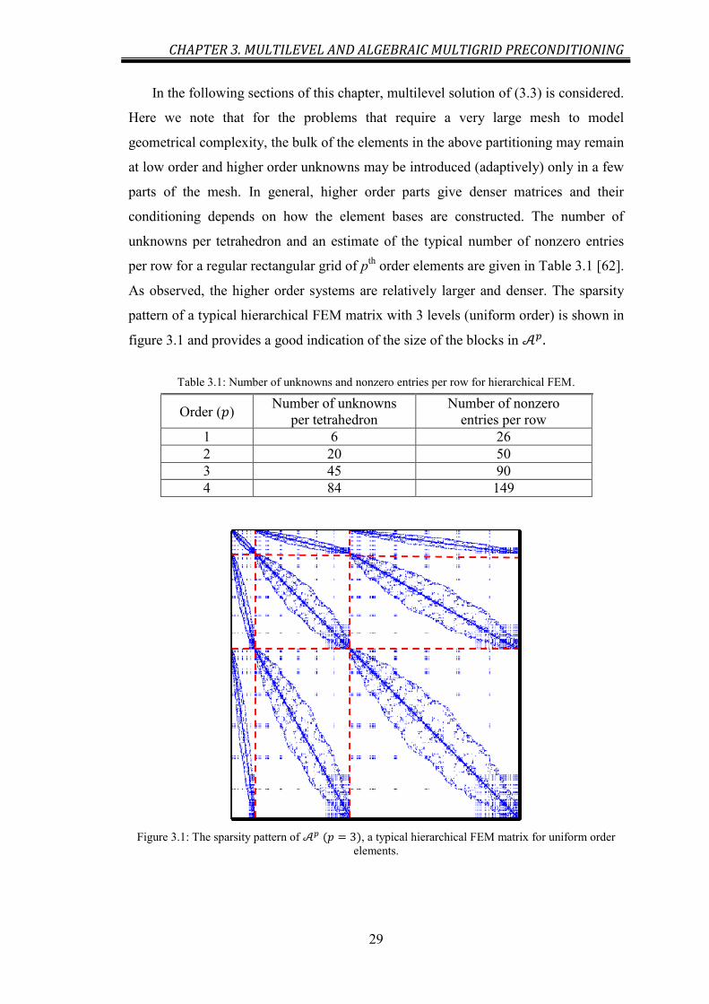
CHAPTER 3. MULTILEVEL AND ALGEBRAIC MULTIGRID PRECONDITIONING
29
In the following sections of this chapter, multilevel solution of (3.3) is considered.
Here we note that for the problems that require a very large mesh to model
geometrical complexity, the bulk of the elements in the above partitioning may remain
at low order and higher order unknowns may be introduced (adaptively) only in a few
parts of the mesh. In general, higher order parts give denser matrices and their
conditioning depends on how the element bases are constructed. The number of
unknowns per tetrahedron and an estimate of the typical number of nonzero entries
per row for a regular rectangular grid of pth
order elements are given in Table 3.1 [62].
As observed, the higher order systems are relatively larger and denser. The sparsity
pattern of a typical hierarchical FEM matrix with 3 levels (uniform order) is shown in
figure 3.1 and provides a good indication of the size of the blocks in
Table 3.1: Number of unknowns and nonzero entries per row for hierarchical FEM.
Order ( ) Number of unknowns
per tetrahedron
Number of nonzero
entries per row
1 6 26
2 20 50
3 45 90
4 84 149
Figure 3.1: The sparsity pattern of , a typical hierarchical FEM matrix for uniform order
elements.

CHAPTER 3. MULTILEVEL AND ALGEBRAIC MULTIGRID PRECONDITIONING
30
3.1.1 Abstract Schwarz Theory and Two-level Scheme
Equation (3.2) can also be written in the following block form
[
] [
] [
] (3.4)
in which
[ ] (3.5)
[
] (3.6)
As shown by (3.4), appears as the square, upper left, submatrix of with
lower right block . The same hierarchical inclusion is followed for the sequence of
matrices . Let and be the dimensions of
and respectively. The rewritten FEM matrix in (3.4) can then be factorized:
[
]
[
] [
] [
]
(3.7)
in which and are identy matrices of size and ,
respectively. According to the multiplicative Schwarz theory and based on the above
factorization, a two-level preconditioning matrix of is:
[
] [
] [
] (3.8)
The term
is called the Schur component of the block .
The above preconditioner is obtained by dropping the coupling term
from the Schur component. In practice, the hierarchical basis functions are partially
orthogonalized and the coupling of the different order basis functions is
weak [47] [62]. The detailed theory of Schwarz method is provided in [63].
An advantage of the above matrix factorization is that it provides a good
understanding of the approximation made by . It is also seen from (3.8) that to
apply the preconditioner to the vector , namely , the inverses of
and are required. However, the overall cost for a preconditioner will be
kept reasonable only if the number of operations involved remains a small multiple of

CHAPTER 3. MULTILEVEL AND ALGEBRAIC MULTIGRID PRECONDITIONING
31
the number of non-zero elements in and . This means that practical two-
level schemes have to rely on an approximate inversion of these matrices, shown
below as and ( ). Usually the approximation consists of a few
iterations of a standard relaxation method, like Jacobi or Gauss-Seidel, so that rapidly
varying components of error are effectively reduced. The Gauss-Seidel has long been
the method of choice within multigrid schemes, because of its effectiveness and
numerically attractive performance on problems of practical interest.
In addition, from a practical point of view, the action of applying should
be defined implicitly by an algorithm, rather than explicitly by building an
approximation to . It can be shown that can be approximated
from the following algorithm:
Algorithm 3.1: The two-level scheme
1. Approximately solve ( ) ;
2. Residual update:
3. Coarsening: “coarse” part of
4. Approximately solve ;
5. Prolongating: prolongation of
6. Residual update:
7. Approximately solve ( ) ;
In line 3, coarsening means that the representation of the field is coarsened by
dropping the entries corresponding to order . Prolongating (line 5) indicates adding
back these entries and setting their values to zero. The coarsening and prolongation
operations are the main components of the multilevel approach that make the
connections between the levels.
3.1.2 From Two Levels to Multilevel
The above construction procedure for a two-level hierarchical matrix can be
extended to all the levels of the multilevel matrix . The multilevel approach is in
fact based on the recursive use of the two-level scheme.
It is known that classical iterative methods like Jacobi and Gauss-Seidel tend to
eliminate the high-frequency components of the residual error in (3.4) more rapidly
than the low-frequency components. The multilevel method is based on this property,
that is, the high-frequency residual components can be eliminated from the higher

CHAPTER 3. MULTILEVEL AND ALGEBRAIC MULTIGRID PRECONDITIONING
32
order unknowns by applying small numbers of relaxation iterations. This step is called
smoothing and provides a cost-effective approximation to the higher order DOFs in
(3.4).
The remaining residual components after applying the smoothing step are
projected onto a coarser level, in which they now have high frequency part to be
eliminated by the action of smoother again. A series of steps can be employed based
on recursive use of the two-level scheme, i.e., the coarser problem is solved
approximately with another application of the two-level scheme on that level, and so
on, until the lowest level is reached, where a more accurate solution is generally
required.
This process computes an improvement in the solution vector and reduces the
residual accordingly. The process is equivalent to the descending half of a cycle for
transferring the residual to coarser levels. The correction at the final step is usually
called the coarse grid correction. When the matrix problem is small enough, the
coarse grid correction can be handled exactly by a direct method. The ascending half
is then continued by applying relaxations again and the result is called a V-cycle p-
type multilevel Schwarz (pMUS) algorithem. Figure 3.2 graphically shows the cycle
for a 4 level pMUS. A solid black circle around a matrix means that it is used in an
application of a relaxation method, such as one step of backward Gauss-Seidel; a solid
gray circle means that it is used in an application of a relaxation method that matches
the one in the descending half, yet may be different from it, to preserve the symmetry
of the overall preconditioning matrix. The box means an exact solution using this
matrix.
Figure 3.2: The V-Cycle p-type Multilevel Schwarz Preconditioner.

CHAPTER 3. MULTILEVEL AND ALGEBRAIC MULTIGRID PRECONDITIONING
33
We define a pair of trivial prolongation and coarsening mappings, and :
[
]
, [ ] (3.9)
where is the identity matrix. “coarsens” the representation of
the field by dropping the entries corresponding to order and “prolongates” the
representation by adding back these entries and setting their values to zero. In
comparison with multigrid methods, the prolongation and projection here are very
simple and independent of domain geometry. Also notice that, by using (3.9), it is
easy to verify that the prolongation and projection satisfy the relation
for . (3.10)
Then the V-cycle method for finding can be described recursively
as follows:
Step 1 (Pre-Smoothing): The smoothing operation is applied to the system of
equations for the highest order unknowns to obtain an approximate
solution , In this step, the high-frequency components in the solution error are
eliminated. The vector is placed in the highest order part of , with the remaining
entries being set to zero.
Step 2: The residual vector corresponding to the approximate solution, is calculated
.
Step 3 (Restriction): The residual vector is projected onto a coarser level using the
restriction matrix: .
Step 4: The residual equation is solved approximately to obtain
the solution vector , corresponding to the representation of the problem at the
coarser level. This step involves solving a smaller problem and takes a shorter time,
because there is a smaller number of unknowns in comparing to .
Step 5 (Prolongation): The solution of the coarser problem is transferred back to the
fine level using the prolongation matrix and the solution obtained in Step 1 is
corrected using .
Step 6: The residual vector corresponding to the recent approximate solution is
updated: .

CHAPTER 3. MULTILEVEL AND ALGEBRAIC MULTIGRID PRECONDITIONING
34
Step 7: (Post-Smoothing): The smoothing operation is applied to the equation
again to correct the values of higher order unknows in vector . This
procedure is called post-smoothing.
We can now state the standard p-type multilevel V-cycle algorithm as follows:
Algorithm 3.2: Standard p-type Multilevel Schwarz:
1. If :
2. Directly Solve order 1:
3. Else if :
4. Pre-Smoothing: ;
5. Residual update:
6. Coarsen:
7. Solve coarse:
8. Prolongate:
9. Residual update:
10. Post-Smoothing: ;
The iteration matrices and used in the algorithm are the Gauss-
Seidel matrices given in (1.8) and (1.9). They act as pre and post smoothers (Step 1
and 7, respectively) for the diagonal blocks . For the standard multilevel V-cycle
method, if the smoother used is symmetric, then the cycle is also a symmetric
preconditioning method. More generally, if two different smoothers are used, one in
the descending path, the other in the ascending path, and they are the transpose of
each other, then the standard multilevel V-cycle method is still symmetric. The
symmetric smoother assumption in the above discussion is important. Without this
assumption, the standard multilevel V-cycle scheme may not be applicable for
preconditioning the Krylov methods that work based on symmetric Lanczos
orthogonalization (discussed in Chapter 4).
3.2 Lowest level Correction
For the multilevel Schwarz method to have satisfactory convergence, the solution
at the lowest level has to be more accurate than at the other levels [62] [60]. The
lowest level correction in Algorithm 3.2 involves solving the following system
(3.11)
In this section, some of the difficulties in solving the above equation for the wave
problem are explained. To discuss the challenges, we first need to be more specific

CHAPTER 3. MULTILEVEL AND ALGEBRAIC MULTIGRID PRECONDITIONING
35
about the structure of matrix . The finite element method discretization of
(2.32) at the Whitney level ( ) leads to the following form for :
(3.12)
in which is the stiffness matrix, is the mass matrix and represents boundary
(surface mass) terms. The elements of the matrices , and are given by
[ ]
∫(
)
(3.13)
[ ]
∫( )
(3.14)
[ ] ∑ ∑
( )
∫
(3.15)
Assuming that the relative permeability tensor is real (passive materials and no
magnetic loss), the stiffness matrix is symmetric positive semidefinite and its
nullspace is spanned by a set of linearly independent vectors corresponding to
irrotational fields. The boundary matrix is symmetric and complex. The mass
matrix is symmetric and will be complex for electrically lossy material (complex
), with a positive definite real part and a small imaginary part (for small losses).
Therefore the negative factor in (3.12) characterizes as an indefinite system,
meaning that the eigenvalues reside on both right and left sides of the complex plane.
Moreover, the condition number of the system typically increases with frequency and
grows as the mesh is refined [64].
In order to better characterize the spectral properties of matrix , we consider
the following related eigenvalue problem, which governs the natural resonances of the
closed system (with the boundary terms omitted):
(3.16)
Assume that the eigenvalue-eigenvector pair satisfies this generalized
eigenvalue problem. The eigenvalues of with negative real part (“negative”
eigenvalues) can be classified into two different sets corresponding to physical and
nonphysical modes of (3.16) [13] [14]. Nonphysical modes are related to the gradient
space of [65] [66] and are usually denoted by the term “Type A” eigenvalues in the

CHAPTER 3. MULTILEVEL AND ALGEBRAIC MULTIGRID PRECONDITIONING
36
literature [13] [14]. Existence of Type A eigenvalues results in serious convergence
issues for Krylov iterative methods, as investigated in pervious works and also shown
by the numerical experiments in Chapter 5.
The other negative eigenvalues of are associated with physical modes of
(3.16) and are therefore of “Type B”. However, they are at frequencies less than the
operating frequency, . Therefore, when the operating frequency is close to a
resonance of the structure, the finite element matrix equation (3.11) can become
highly ill-conditioned.
For the Whitney space , the gradient and rotational spaces are not separated and
nonphysical negative eigenvalues of the system cannot be easily preconditioned into
positive eigenvalues [62]. That is the main reason for the slow convergence exhibited
by conventional iterative schemes applied to the lowest order block, , with
standard preconditioners like incomplete Cholesky (IC) and Gauss-Seidel [65].
In the conventional pMUS algorithm, is decomposed exactly to avoid this
difficulty. However, many modern problems involve very complex geometries,
making the number of elements after meshing extremely large. For realistic three
dimensional problems, a large number of Whitney degrees of freedom can arise after
discretization and the lowest level linear system is itself often very large. Therefore,
the decomposition of , if not impossible to apply, will become the bottleneck.
Consequently, the efficient, robust (e.g., with respect to the properties of the PDE)
and fast treatment of the lowest level correction remains a difficulty for the pMUS
algorithm.
As possible replacements for the direct treatment, multigrid methods are among
the most efficient approaches for approximate inversion of large linear systems. They
follow the same idea as pMUS: damping errors by utilizing multiple resolutions in a
recursive scheme. High-energy and oscillatory components are effectively reduced
through a simple smoothing procedure, while the low-energy components are tackled
using a lower resolution version of the problem (coarse grid).
For large scale problems, the geometric multigrid (GMG) methods can be used
for solving (3.11) if we have a nested sequence of meshes [56] [57] [67]. By defining
appropriate transfer operators, the FE spaces are linked together. Recursive
application of a two grid process can be applied by performing pre-smoothing steps

CHAPTER 3. MULTILEVEL AND ALGEBRAIC MULTIGRID PRECONDITIONING
37
on the fine system, and then restricting the residual on the coarse mesh. On the
coarsest level the coarse system is solved (exactly) and the defect is prolongated on
the fine level. Finally, post-smoothing steps are performed.
When nested meshes are not available, algebraic multigrid (AMG) methods can
be used instead. Eliminating the decomposition of by the application of AMG is
investigated in this thesis.
3.2.1 Algebraic Multigrid for the Problem
In contrast to GMG, where a grid hierarchy is required explicitly, algebraic
multigrid (AMG) is able to define the prolongation operators (and construct the
corresponding matrix) in a pure algebraic way. AMG operates more on the level of
the matrix than of the underlying nested FE meshes. The crucial point in the
construction of the algebraic methods is the numerical effort of the coarsening process
and the construction of appropriate transfer operators. The challenge is to construct an
AMG method with a good convergence rate but rather low costs in the setup and the
application.
Classical algebraic multigrid methods have had a lot of success on Poisson
problems, obtained from scalar, nodal, basis functions. Nodal AMG methods, also
known as scalar AMG, simply apply a relaxation scheme to a hierarchy of
algebraically constructed coarse-grid problems. Efficient implementations of AMG
have been under intensive research in the last decade and several well-established
software libraries have been developed [17].
However, a unique difficulty in solving (3.11) with AMG arises from the nature
of the curl-curl operator. Traditional AMG methods are adapted only to the Laplacian
operator on and deal badly with the curl-curl operator [23] [75]. The first
serious and practical AMG approach for problems in was made in 2002 by
Reitzinger and Schoberl [23]. The principal idea of their method is to maintain the
representation of a discrete gradient and its relationship to the discrete curl-curl
operator on coarse meshes. This can be achieved by creating two multigrid hierarchies
for the nodes and edges of the mesh and aggregating the edges via nodal aggregation,
in such a way that necessary conditions on the prolongation operators are imposed.
After constructing the AMG hierarchy, each coarser version of has a nullspace

CHAPTER 3. MULTILEVEL AND ALGEBRAIC MULTIGRID PRECONDITIONING
38
spanned by the gradient of a set of linearly independent scalars over the coarse grid.
The proposed method is easy to compute and has low multigrid operator
complexity [68], but the prolongator has poor approximation properties and the
convergence rates suffer [25] [68]. An improved version of [23] can be found
in [69] [70] [25], where a better prolongation was proposed, with mesh-independent
convergence rates. These method however require two coarsening procedures and
hybrid smoothers at every level to handle nonelliptic discretization problems and
efficient multigrid methods developed for scalar AMGs are not often directly
applicable.
3.3 Auxiliary Space Preconditioning
Recently, Hiptmair and Xu proposed an innovative approach for solving
systems, known as HX auxiliary space preconditioning [72] [73]. The approach relies
on a decomposition of Whitney vector fields and employs the framework of the
auxiliary space method. In contrast to applying coarsening to the edge unknowns, it
uses “edge to node” projection and solves approximate problems in auxiliary spaces
defined on the nodes of the original mesh. This property significantly simplifies the
computations and, more importantly, allows us to makes use of the proven ability of
scalar AMG for nodal FEM problems.
The idea of auxiliary space preconditioning (ASP) is to invert approximately the
curl-curl operator by transferring the problem into subspaces in which scalar AMG
can be applied. Although this method was proposed for the positive-semidefinite case,
which occurs in time-domain, quasi-static problems, extensive numerical experiments
reported in this thesis demonstrate that it is also efficient and robust for the frequency-
domain problems, both quasi-static and full-wave.
3.3.1 Whitney Space Decomposition
The present section summarizes the main ingredients used to derive the auxiliary
space preconditioner (see [71] [72] [74] [75] for details).

CHAPTER 3. MULTILEVEL AND ALGEBRAIC MULTIGRID PRECONDITIONING
39
a) Regular Decomposition
Let be the space spanned by the lowest order edge element basis
functions on a tetrahedral mesh (the Whitney space). There is an associated space
of piecewise linear, scalar functions on the same mesh and it is known
that is the irrotational subspace of [75] [78].
It is also known that for every , there exists a member in the
space [ ] with the same curl, i.e. [75]. This suggests
that functions in can be represented approximately using functions in and
. With the purpose of defining an auxiliary space preconditioner, we first need
to define the Nedelec interpolation operator in order to map vectors of into
as follows:
∑( ∫
)
(3.17)
where is the Whitney basis function defined in Table 2.2 and is a vector tangent
to edge .
Suppose now that . Then it follows that there exists such
that . For such a , it can be shown that . It
follows that:
(3.18)
Therefore,
(3.19)
Since and has a zero curl, it can be represented by for some
. The following Whitney space decomposition, known as a regular
decomposition [20], can be achieved:
(3.20)
Assuming that stands for a constant independent of the mesh size and in
accordance to the norms defined in Section 2.4, the following inequality holds [75]:
‖ ‖ ‖ ‖ ‖ ‖ (3.21)

CHAPTER 3. MULTILEVEL AND ALGEBRAIC MULTIGRID PRECONDITIONING
40
b) Hiptmair-Xu Decomposition
The regular decomposition in (3.20) is in fact semi-discrete, since it involves the
term that, in general, is not a finite element function. The challenge is to
convert (3.19) into a purely discrete decomposition with some stability condition
similar to (3.21). There are several ways to further approximate the non-discrete
component [75]. In the Hiptmair-Xu (HX) decomposition, it is achieved by
incorporating another high frequency, “small” component.
For the HX decomposition, we introduce the space of vector “nodal” functions,
. These are vector functions that, unlike Whitney basis functions, are
both normally and tangentially continuous from one element to the next and are fully
first-order in each element. For any there exists that
satisfies [75]:
‖ ‖ ‖ ‖ ‖ ‖ (3.22)
Defining the small contribution , we have to
be substituted in (3.20). Therefore, the space , the scalar space and the vector nodal
space are linked by the following result: for any there exists and
such that:
(3.23)
and the following stability estimate holds (the proof can be found in [75]):
‖ ‖ ‖ ‖ ‖ ‖ ‖ ‖ (3.24)
Table 3.2 summarizes the spaces involved in the HX decomposition and gives a
graphical representation of the basis functions for the FE spaces.

CHAPTER 3. MULTILEVEL AND ALGEBRAIC MULTIGRID PRECONDITIONING
41
Table 3.2: Spaces involved in the HX decomposition, along with corresponding members and basis
functions illustration.
Hilbert Space [ ]
Members
FE space 1st order Scalar Space Whitney Space 1st order Vector Space
Relations
Members
Basis
illustration
3.3.2 Method of Subspace Correction
Based on the HX decomposition, we are able to represent the space as the
summation of subspaces. This splitting concept also suggests that it might be possible
to solve the problem approximately by solving related problems on the auxiliary
spaces and . Therefore, the original problem in (3.11) can be split into sub-
problems if we can find appropriate mapping operators between the spaces. The sub-
problems are relatively easier to solve, since they represent smaller problems in nodal
spaces. Providing that required projection operators to the subspaces are available,
different components of error can be captured separately by these subspaces. Solution
components can then be combined in various versions that will be described later.
To realize the preconditioners for the finite element matrix, the decomposition
discussed in the previous section should be adapted to a matrix setting too. We use the
usual nodal, interpolatory basis in and , as well as the Whitney edge basis in .
Then functions and can be represented by column vectors of node and
edge values, respectively. But first the mapping operators are introduced.
3.3.3 Mapping Operators
The matrix representation of the mapping operator from to is commonly
called the discrete gradient matrix, denoted by sparse matrix . It is simply the node
to edge mapping matrix with entries of -1 and 1 per row. This matrix is readily

CHAPTER 3. MULTILEVEL AND ALGEBRAIC MULTIGRID PRECONDITIONING
42
available since it describes the edges of the mesh in terms of its vertices. If is an
edge from node to , then the only two non-zero entries of in the row
corresponding to are [13] [75]
[ ] [ ] (3.25)
To preserve symmetry, we use the transpose, , to map backwards from to
.
For we use the basis for each Cartesian component of the vector and
represent by a column vector in which nodal values of the , and
components occupy 3 successive blocks. Then the operator becomes a sparse
matrix which also has a block form:
[ ] (3.26)
Each block has the same dimension and sparsity pattern as , i.e., two nonzero
entries per row [75]. If is an edge connecting nodes and , with coordinates
and , then
[ ] [ ]
(3.27)
As observed, the two nonzero values for row of , are identical. It can be
shown that their value is also equal to the th row of the product
, where
[ ] is a vector containing the coordinates of the nodes.
Similarly for and :
[ ] [ ]
(3.28)
and
[ ] [ ]
(3.29)
We use to map backwards, from to .
3.3.4 Discretized Operators for the Auxiliary Spaces
Along with these matrices, we also need discretized operators representing the
original bilinear form in each auxiliary space. Corresponding to the bilinear form
(2.32), we introduce the following weak form for the problems defined on auxiliary
spaces and :
CHAPTER 3. MULTILEVEL AND ALGEBRAIC MULTIGRID PRECONDITIONING
43
(3.30)
(3.31)
In (3.31), stands for a modified version of (2.32), in which the
wavenumber is replaced by
in the volume integral only. Setting
results in exactly the original weak form. The reason for this complexification is
explained later, in Section 3.5.
The above problems are equivalent to
(3.32)
(3.33)
We can now rephrase the problem of solving Maxwell’s equations as the
following:
(3.34)
(3.35)
in which
(3.36)
(3.37)
and
(3.38)
(3.39)
Following the standard procedure, a set of linearly independent, first-order, nodal
basis functions and can be introduced for expansion
of and . The above problems may be reduced to the following algebraic matrix
equations:
(3.40)
(3.41)
In which

CHAPTER 3. MULTILEVEL AND ALGEBRAIC MULTIGRID PRECONDITIONING
44
[ ] ; [
] (3.42)
[ ] ; [
] (3.43)
Each of the problems (3.42) and (3.43) are in fact equivalent to (3.11), but solved
in the auxiliary spaces. It can be shown that the square matrices and
for the
auxiliary problems can also be computed by the Galerkin product:
(3.44)
(3.45)
where is the system matrix that is obtained instead of when is used
instead of . The numerical cost for building each of these is roughly
equivalent to four matrix-vector products of [79].
3.4 Damped Operator Preconditioning
It was mentioned in Section 3.2 that the spectral properties of the matrix
associated with the discretization of the vector wave operator at level 1 makes
extremely difficult the convergence of iterative solvers applied to the related linear
system. As explained by equations (3.13) to (3.15), the discretization of (2.32) at the
Whitney level leads to the following form for :
(3.46)
Referring to the discussion in Section 3.2, the negative factor in relation
(3.46) makes indefinite. As the wavenumber increases beyond each physical
resonance, more negative eigenvalues appear and the indefiniteness of system causes
slower convergence of iterative solvers.
Although the linear algebra theory for definite linear systems is well-developed, it
is not the case for indefinite linear systems. In the last few decades, much effort has
been directed towards the construction and implementation of robust and efficient
preconditioners for indefinite linear systems. Particularly in the last few years,
physics-based preconditioners have attracted the attention of many
researchers [80] [81] [82] [83] [84]. The main idea is to include information related to
the physical properties of the problem and also the structure of the operators, when

CHAPTER 3. MULTILEVEL AND ALGEBRAIC MULTIGRID PRECONDITIONING
45
trying to build a preconditioner. Among the main contributions, the Shifted Laplace
Preconditioner (SLP) [80] has received much attention.
Essentially, the idea in SLP is to build the preconditioner based on a complex
version of the original operator. In fact, positive definiteness of the overall system is
reinforced through the introduction of a fictitious dissipative term into the operator
from which the preconditioner is derived. The approach has been applied successfully
by Erlangga et al. to the wave-like problems described by the scalar Helmholtz
operator [80]. To the best of our knowledge, it has not previously been applied to the
curl-curl operator.
Following the idea of SLP, it would be beneficial to use a preconditioner based on
a damped operator version of (2.32) by introducing a complex factor in the
wavenumber. The preconditioner matrix is then obtained from discretization of (2.32),
in which the complex modification is applied to
. The boundary
conditions are left unchanged, i.e., the preconditioner is built from:
(3.47)
Since the convergence of Krylov methods is closely related to the spectrum of the
iteration matrix, the favourable spectrum of the preconditioned matrix ( )
will give some insights into the improved convergence rate. Numerical evidence
shows that, unlike the spectrum of the unpreconditioned system, the eigenvalues of
( )
are mapped to a roughly circular pattern in the right-hand half of the
complex plane. In fact, similar to the positive effects of spectral changes for the
Helmholtz equation preconditioned by the Shifted Laplace operator [81], when all the
eigenvalues of the ( )
are located in the right half plane, better convergence
of an iterative solver can be ensured. In addition, the eigenvalues are mostly shifted
away from the origin and clustered around 1. This suggests that leads to a better
preconditioner than . Adding an artificial dissipative term also implies that
computing the approximate inverse of can be performed more efficiently using
multigrid methods [80].
According to this analysis, one strategy is to build the complete auxiliary space
preconditioner from instead of . That would mean using
for the smoothing
step and for building and
in (3.44) and (3.45). However, experiments show

CHAPTER 3. MULTILEVEL AND ALGEBRAIC MULTIGRID PRECONDITIONING
46
that it is most effective for damping the rotational type errors and using for
smoothing and for building actually worsens the performance of the
preconditioner. Therefore, it is used only to build in (3.45).
The convergence of an iterative Krylov subspace solver applied to the linear
system with SLP and AMG will be independent of the mesh refinement and
dependent (but in a weaker way than without the preconditioner) on the wavenumber
. The convergence is also clearly affected by the choice of the parameter .
Following numerical studies, we propose the choice , which leads to an
efficient and robust preconditioning method.
What is important for the convergence of Krylov subspace methods is that, though
the spectrum of the preconditioned system is nicely clustered, some eigenvalues still
lie close to zero. With an increase in the wavenumber, the number of eigenvalues
around zero appears to increase also.
3.5 ASP Preconditioners for the Wave Equation
We can now present efficient methods for approximately solving using
ASP. Depending on different ways of connecting the 3 FE spaces involved, the
following symmetric preconditioners are considered at the lowest level:
3.5.1. Additive Preconditioner
In order to approximate , we can first use an SSOR preconditioner to
damp small components in (3.23) like . This takes the form where
(see equation (1.13).
After the smoothing step, we can transfer the residual into each auxiliary space
and solve the residual equation in each space. Exact inversion of and
is
expensive, but fortunately scalar AMG (which will be defined in Section 3.7) is
effective in approximately inverting and each of the three diagonal blocks of
:
(3.48)
(3.49)
(3.50)

CHAPTER 3. MULTILEVEL AND ALGEBRAIC MULTIGRID PRECONDITIONING
47
We call the approximate inverses of these four matrices ,
, and
,
respectively. Now we can approximately compute . The main body of the
resulting preconditioner consists of three components:
1. Smoothing in the space using sweeps of SSOR, expressed by
.
2. Approximate solution in the kernel of (with a nodal AMG solver),
expressed by .
3. Approximate solution in the vector nodal counterpart of (with nodal AMG
solver), expressed by
, .
Based on the framework of auxiliary space correction, solutions from each
problem are assembled to give a correction in the space . In the simplest method,
the four corrections for a given residual can be added, resulting in the following
additive preconditioner with operations that can be performed in parallel to each
other:
∑
(3.51)
The additive preconditioner (3.51) is coded in the following algorithm. The
approximate inverse of defined by this algorithm is denoted .
Algorithm 3.3: Additive Preconditioner
1. SSOR:
2. Auxiliary spaces: ∑
3. Solution update:
3.5.2. Multiplicative V-cycle Preconditioner
Another way to assemble the corrections is a multiplicative V-cycle that splits the
SSOR correction in Algorithm 3.3 into backward and forward Gauss-Seidel iterations
in the downward and upward sides of a V-cycle. This version performs better than the
additive approach in general:

CHAPTER 3. MULTILEVEL AND ALGEBRAIC MULTIGRID PRECONDITIONING
48
Algorithm 3.4: Multiplicative V-cycle ASP Preconditioner
1. Backward GS:
2. Residual update: ;
3. Auxiliary spaces: ∑
4. Residual update: ;
5. Forward GS:
6. Solution update:
The approximate inverse of defined by Algorithm 3.4 is denoted . In an
alternative approach, one may consider a multiplicative version also for the 4
auxiliary space corrections by repeating steps 2, 4 and 5 for each nodal correction.
However, considering the size of problems and the relatively higher cost of Gauss-
Seidel iterations and residual updates for edge DOFs, parallel computation of nodal
corrections would be numerically more attractive.
3.5.3. Multiplicative W-cycle Preconditioner
Since the work done at lines 2-6 of the previous algorithm is relatively
inexpensive (comparing to higher order smoothing steps in pMUS) and yet important
to the accuracy of coarse level correction, it is also worth considering the following
W-cycle alternative. In practice, the best performing preconditioner arises from a
multiplicative W-cycle. The approximate inverse of defined by the following
algorithm is denoted .
Algorithm 3.5: Multiplicative W-cycle ASP Preconditioner
1. Backward GS:
2. Residual update: ;
3. Auxiliary spaces: ∑
4. Residual update: ;
5. Backward GS:
6. Residual update: ;
7. Auxiliary spaces: ∑
8. Residual update: ;
9. Forward GS:
10. Residual update: ;
11. Auxiliary spaces: ∑
12. Residual update: ;
13. Forward GS:
14. Solution update:

CHAPTER 3. MULTILEVEL AND ALGEBRAIC MULTIGRID PRECONDITIONING
49
3.6 ASP Preconditioners for the T- Method
The matrix equation of the formulation (Section 2.5.2) at the lowest level,
, is further partitioned into rows and columns corresponding to T and
basis functions:
[
] {
} {
} (3.52)
Following the idea behind ASP, the problem is transferred to a number of
auxiliary function spaces. For the unknown , represented by Whitney edge elements
over the edges of the mesh, the same auxiliary spaces and are involved.
Equivalent problems, similar to (3.40) and (3.41) are constructed for the part of the
field. However, since this exists only inside the conducting regions and vanishes
tangentially on the surface, the corresponding auxiliary spaces are defined by just the
nodes interior to .
We define matrices and [ ] that map column vectors
representing functions in and , respectively, to column vectors of the same size
as that represent fields of order 1. Specifically, they map to the T partition
of , representing functions in the Whitney space inside . In fact, since there are
no edge functions for the tree edges in , they map just to cotree edges, but the
matrix entries are the same as in (3.25) and (3.27) to (3.29).
The part of the field also has to be accomodated and for this we use the
auxiliary space that is spanned by the piecewise linear scalar functions of the whole
mesh (not just the mesh in ). The matrix for this space is . Like , it is a
discrete representation of the gradient operator.
The matrices , , which are the auxiliary space counterparts of
, are given by
(3.53)
Approximate inverses of these five matrices are also denoted , .
We can now construct the ASP algorithms based on V-cycle and W-cycle
approximation for solving . The effective multiplicative preconditioners are
very similar to Algorithm 3.4 and Algorithm 3.5, but with 5 auxiliary space

CHAPTER 3. MULTILEVEL AND ALGEBRAIC MULTIGRID PRECONDITIONING
50
corrections instead of 4. For example, in the multiplicative V-cycle preconditioner,
line 3 of Algorithm 3.4 is modified as follows:
∑
(3.54)
and similarly for the W-cycle approximation in lines 3, 7 and 11.
3.7 Standard AMG Methods for Poisson Problems: Nodal AMG
Multigrid methods are well known to be cost effective for elliptic problems. AMG
is seen by many as one of the most promising methods for solving the large-scale
problems that arise in this context [74] [75] [77]. Here we present the basic principles
and techniques for solving nodal problems using AMG. Consider a problem of the
form
, (3.55)
The approximate inverses of these four nodal matrices that were denoted by
( ) in the additive and multiplicative algorithms are never formed
explicitly. Instead, the product is found by scalar AMG:
( )
( ) (3.56)
The third argument, 0, is the AMG level number (see below). The central idea in
scalar AMG is that error components not eliminated by relaxation must be removed
by coarse-grid correction. Simple relaxations reduce high frequency error components
efficiently, but they are very slow at removing low energy components. However, the
error that remains after relaxation can be approximated more accurately on a coarser
grid. This is done by solving the residual equation on a coarser grid, then interpolating
the error back to the fine grid and using it to correct the fine-grid approximation. The
coarse-grid problem itself can be solved by a recursive application of this method.
One iteration of this process, proceeding through all levels, results in the multigrid
cycle.
In AMG the main task is to determine a coarsening process that approximates the
error that a chosen relaxation cannot reduce. The grid that appropriately represents
coarse degrees of freedom for the original problem is called a “virtual” finite element
mesh. In order to construct and connect these virtual grids together, several

CHAPTER 3. MULTILEVEL AND ALGEBRAIC MULTIGRID PRECONDITIONING
51
components are required. Using superscripts to indicate the level number, so that
correspond to the real tetrahedral mesh, the components that AMG needs are as
follows:
1) (virtual) Grids: .
2) A relaxation scheme for each level, like Gauss-Seidel iteration.
3) Grid transfer (prolongation) operators:
,… , ,
, which are sparse,
rectangular matrices for relating the nodes of a coarse grid to the nodes of a
finer grid.
4) Grid operators:
, … ,
, , which are a series of progressively
smaller, square, sparse matrices. These matrices are defined using the
prolongation operators:
(
)
Once these components are defined, the recursively defined cycle of scalar AMG
is as follows:
Algorithm 3.6: scalar AMG (
)
1. If (the coarsest level considered):
2. Solve exactly: ( )
3. Else:
4. Backward GS: ( )
5. Residual update: ;
6. Coarsen: ( )
7. Coarse solution: 8. Prolongate:
9. Residual update:
;
10. Forward GS: ( )
11. Solution update:
The preparation of the components of AMG is done in a separate setup phase. In
the setup phase, before the start of the Krylov iteration, the matrices are formed
explicitly, and then the AMG matrices and
. These quantities are used
repeatedly throughout the iteration.
Algorithm 3.7: AMG setup Phase
1. Set
2. Partition into disjoint sets and .
3. Set
4. Define prolongation matrices

CHAPTER 3. MULTILEVEL AND ALGEBRAIC MULTIGRID PRECONDITIONING
52
5. Set (
)
6. If is small enough for factorizing
, set and stop.
Otherwise, set and go to step 2.
The details of steps 2 and 4 are given in [17].
Adding more levels reduces the memory required for the coarsest level exact
factorization, but sacrifices the performance if coarsening is too great. Generally,
adding more levels should be continued provided that the virtual AMG meshes can
adequately represent field variations on the scale of the wavelength (for wave
problems). We can estimate the “edge length” on a virtual mesh as √
,
where is the average edge length in the original mesh
and
is the ratio of the number of nodes in the original mesh to the number of
nodes in the virtual mesh. A value of for the above measure has shown
satisfactory performance in our numerical results (see Chapter 5).
3.8 Multilevel and Algebraic Multigrid Cycles: pMUSASP
In this section, I introduce the Multilevel/ASP/AMG version of the pMUS
method explained in Algorithm 3.2 for solving (3.2). The approach is called
and employs the AMG treatment at the lowest level instead of the direct
solve. The function returns an approximation to , where
is a vector of the appropriate length. It involves primarily the application of
forward and backward Gauss-Seidel (GS). The algorithm is given
recursively as follows:
Algorithm 3.8: Multilevel/Algebraic Multigrid pMUS:
1. If : 2. Solve order 1:
3. Else if : 4. Backward GS: ; 5. Residual update: 6. Coarsen: 7. Solve coarse: 8. Prolongate: ; 9. Residual update: 10. Forward GS: ;

CHAPTER 3. MULTILEVEL AND ALGEBRAIC MULTIGRID PRECONDITIONING
53
The vectors and are blocks of and , respectively, corresponding to the
partitions in (3.2). The operation is one of the algebraic approximations
described by Algorithms 3.3 to 3.5, i.e. ,
or .
The call with (Algorithm 3.4), then,
initiates the V-cycle shown in Figure 3.3, during which GS is applied to the sequence
of matrices shown – backward GS on the downward portion, and forward GS on the
upward portion. This completes the V-cycle approximation of . The output
is used in every preconditioning step of a Krylov solver that solves .
Figure 3.3: The V-cycle version of . Dashed arrows imply a series of steps with
decreasing (downward) or increasing (upward) matrix superscripts.
Since the most computationally intensive part of the preconditioner is pMUS, it
has been found beneficial to execute the ASP/AMG part more than once in each
cycle, because this reduces the number of Krylov iterations at relatively small
additional cost. This gives the extended W-cycle shown in Figure 3.4, in which
Algorithm 3.5 for is used. Note that the backward and forward GS
has been arranged to preserve the symmetry of the overall preconditioner. Other
symmetric arrangements are also possible.

CHAPTER 3. MULTILEVEL AND ALGEBRAIC MULTIGRID PRECONDITIONING
54
Figure 3.4: The W-cycle version of .
The Multilevel/ASP/AMG version of pMUS for the problem is very
similar to Figure 3.3 and Figure 3.4. The only difference is that the ASP/AMG parts
involve parallel approximation of five nodal systems instead of four.

CHAPTER 4
Krylov Methods and Deflation
In this chapter, Krylov subspace methods for solving the complex-
symmetric linear system of the form
(4.1)
are presented. Matrix and vector correspond to the adaptive systems (2.36) or
(2.45) with the block structure pattern defined in (3.3) . Krylov subspace methods are
extensively used for the iterative solution of large linear systems of equations and in
particular those arising from discretizations of Maxwell’s equations. We begin our
discussion in Section 4.1 by introducing the Krylov subspace approach and discussing
methods based on Lanczos and Arnoldi algorithms. In Section 4.2, preconditioned
Krylov methods for complex symmetric matrices are presented by extending the
standard conjugate gradient approach. Next, in Section 4.3 the method of Generalized
Minimal Residual is explained. Section 4.4 introduces the concept of deflation and
how it can be used in designing more robust Krylov subspace iterative methods.

CHAPTER 4. KRYLOV METHODS AND DEFLATION
56
4.1 Krylov Subspace Methods
The Krylov subspace iteration methods are based on the construction of a Krylov
subspace, i.e.
(4.2)
where is the residual corresponding to the initial guess vector . The
dimension of is equal to and increases by one at each step of the approximation
process.
The idea of designing iterative methods based on the Krylov subspace can be
outlined as follows. For an initial solution , approximation to the solution of
(4.1) is computed in the th iteration as
(4.3)
For this purpose, all the Krylov subspace methods construct the basis vectors
where
[ ] (4.4)
With the residual , the expression for the solution and residual at
the th step can be written as:
(4.5)
(4.6)
where . From (4.5) and (4.6) we observe that Krylov subspace methods rely
on constructing the basis of and the vector . The differences among the various
algorithms are the ways of computing these vectors. If the components can be selected
properly, the approximate solution can be very close to the exact solution for even
a small number of iterations ( ).
In order to determine the subspace, many algorithms have been proposed. In
general we identify two methods that can be used for constructing the basis: the
Symmetric Lanczos method and the Arnoldi method. In the following sections, we
present some Krylov subspace algorithms based on these methods that are used in
numerical simulations in this thesis. In particular, we discuss the Conjugate Gradient
(CG) and its extension to the complex systems, Minimal Residual (MINRES) and
Generalized Minimal Residual (GMRES) algorithms.

CHAPTER 4. KRYLOV METHODS AND DEFLATION
57
We end this section by describing some of the notation. For complex vector
, the complex-conjugate transpose is denoted by . By ⟨ ⟩ we
denote an inner product between the vectors . In this case, the induced
vector norm is ‖ ‖ √⟨ ⟩ . We also use a different bilinear functional denoted
by which is used to derive a CG-like method for complex symmetric
matrices. When , the complex vectors and are called conjugate
orthogonal. The unit vector is defined by [ ] . For a vector
that is partitioned as (3.3), we refer to the first partition as [ ]
4.2 The Symmetric Lanczos Process
Here we assume the matrix to be Hermitian. Given and , the symmetric
Lanczos process [15] computes a sequence of Lanczos vectors and scalars and
for , starting from ‖ ‖ and . Defining , the
process satisfies the following three-term recurrence:
(4.7)
in which
(4.8)
and chosen such that
‖ ‖ (4.9)
In exact arithmetic, the vectors are orthogonal (i.e. ⟨ ⟩ for ) and
the process stops when for some . In matrix form, for
, (4.7) is:
(4.10)
where [ ] and is the following tridiagonal matrix:
(4.11)

CHAPTER 4. KRYLOV METHODS AND DEFLATION
58
An important property of the Lanczos vectors in is that they lie in the Krylov
subspace defined by (4.4). Hence, at iteration , we look for an
approximate solution . The associated residual vector is
(4.12)
By choosing in a way to make small, we can arrive at different iterative
methods for solving the linear system. Since is theoretically orthonormal, we can
find by solving
(4.13)
Two particular ways of solving (4.11) lead to CG [85] and MINRES [85], which
are established methods for symmetric systems. They both exploit the three-term
recurrent scheme for delivering an efficient Krylov subspace method for symmetric
systems, but each method has a different minimization property that suggests a
particular factorization of .
4.2.1 Conjugate Gradients for Complex Symmetric Systems
The Conjugate Gradient (CG) method was introduced for solving when
is Hermitian Positive Definite (HPD). CG iterations are characterized by minimizing
‖ ‖ , where
‖ ‖ √⟨ ⟩ (4.14)
The algorithm can be derived directly from its equivalent Lanczos formulation
that computes the solution of the tridiagonal system progressively by
using Gaussian elimination without pivoting [15]. The factorization of matrix
can be written in the form
(4.15)
and the approximate solution at th step is :

CHAPTER 4. KRYLOV METHODS AND DEFLATION
59
(4.16)
Letting
(4.17)
and
(4.18)
then (4.16) is
(4.19)
However, computation of (4.19) can be done progressively, since the last column
of the matrix , shown by , and last entry of vector , shown by , can be
obtained from the previous values following simple updates:
(4.20)
(4.21)
As a result, can be updated at each step as
(4.22)
and the residual vector of the approximate solution is such that
(4.23)
The above relations give us an algorithm which is usually called the direct version
of the Lanczos algorithm [15]. The residual vectors for this algorithm are orthogonal
to each other due to equation (4.23) and the vectors are also -orthogonal,
meaning that is a diagonal matrix [15]. As a consequence, an efficient version
of the conjugate gradient algorithm (in terms of required storage) can be derived by
imposing these orthogonalities, in which based on (4.22) the new approximation
vector at every iteration is expressed as
(4.24)
where is the search direction and
(4.25)
The residual vectors then satisfy the recurrence
CHAPTER 4. KRYLOV METHODS AND DEFLATION
60
(4.26)
For all to be orthogonal, the necessary condition is that ⟨ ⟩ . Thus
⟨ ⟩ (4.27)
Since the next search direction is a linear combination of and , we find
that
⟨ ⟩
⟨ ⟩ (4.28)
Also because ⟨ ⟩ , we have
⟨ ⟩
⟨ ⟩ (4.29)
Equations (4.24) to (4.29) completely describe all the necessary calculations at
every iteration of the CG algorithm. The implementation requires only one product
for some vector and a small amount of computations for computing the vectors
, and . If is HPD, the norm of the residual vector ‖ ‖ also reduces
monotonically at each iteration, which makes CG highly efficient and preferable.
However, for non-Hermitian matrices, like the global FE matrix of the vector wave
equation, the algorithm may not converge. This is because the orthogonality condition
(4.27) cannot be satisfied in general.
One simple remedy for complex-symmetric systems ( ) is to replace the
orthogonality condition by the so-called conjugate orthogonality condition based on
the following inner product
. (4.30)
In this case, the vectors also form a basis for .
Furthermore, the vectors are conjugate orthogonal:
. ( ) if (4.31)
Therefore, solution can be constructed by requiring the residual to be
conjugate orthogonal to . This results in an algorithm which is similar to
CG, but with the Hermitian inner product being replaced by (4.30). The algorithm,
called conjugate orthogonal-conjugate gradient (COCG) is as follows:

CHAPTER 4. KRYLOV METHODS AND DEFLATION
61
Algorithm 4.1: Conjugate Orthogonal Conjugate Gradient (COCG)
1. Set the initial guess: . Compute .
2. Set
3. for
4. ⁄
5.
6. (Stop if accurate enough)
7. ⁄
8.
9. End
Algorithm 4.1 also preserves the nice property that it requires only one matrix-
vector multiplication and a few vector updates per each iteration. However, it is no
longer optimal in a sense that the error at every step is not minimal. This means that
the error is not monotonically decreasing. The condition is also restrictive in
that it only allows incorporation of a symmetric preconditioner.
4.2.2 Preconditioned COCG
The convergence of Krylov methods like COCG might be very slow for the type
of equations defined in (4.1), which are generally ill-conditioned systems. A Krylov
subspace method is usually combined with a preconditioner to reduce the total
number of iterations. Iterative solutions can be accelerated if well-chosen
preconditioners are available. Our objective in Chapter 3 was to find appropriate
(symmetric) preconditioners which can easily be used with Krylov subspace methods
and also reduce the total number of iterations.
Suppose that represents a preconditioner whose inverse is easy to compute
(like the multilevel/algebraic multigrid in Algorithm 3.8). By employing the
preconditioner, instead of solving the original linear system (4.1), we solve a better
conditioned system
(4.32)
Therefore, the preconditioned Krylov subspace method is defined by constructing
iteration such that
(4.33)

CHAPTER 4. KRYLOV METHODS AND DEFLATION
62
One important aspect of incorporating a symmetric preconditioner is that a
preconditioned version of COCG can be derived in a straightforward way. Supposing
that has Cholesky factorization and by redefining the variables
. , ,
(4.34)
we can directly apply COCG to (4.32), yielding the following algorithm:
Algorithm 4.2: Preconditioned Conjugate orthogonal Conjugate Gradient (PCOCG)
1. Set the initial guess: . Compute
2. ,
3. for
4. ⁄
5.
6. (Stop if accurate enough)
7.
8. ⁄
9.
10. End
In fact, the iterates •_produced by the above algorithm and Algorithm 4.1 applied to
the system are identical, provided that the same initial guess is
used.
If is very far from the nearest positive definite matrix, Algorithm 4.2 may
converge slowly. When is ill-conditioned, the Cholesky factorization of might
fail or be numerically unstable. A better approach is to use a more numerically stable
factorization for solving (4.13).
4.2.2 Conjugate Orthogonal Minimal Residual, CO-MINRES
The CG method and the minimal residual method (MINRES) are both Krylov
subspace techniques for the iterative solution of Hermitian linear equations. While CG
is commonly used when the matrix is positive definite, MINRES is generally
reserved for indefinite systems. MINRES [11] [85] is characterized by the following
minimization:
= where minimizes ‖ ‖ (4.35)
Thus, MINRES minimizes ‖ ‖ within the th Krylov subspace. Since this
minimization is well-defined regardless of the definiteness of , MINRES is
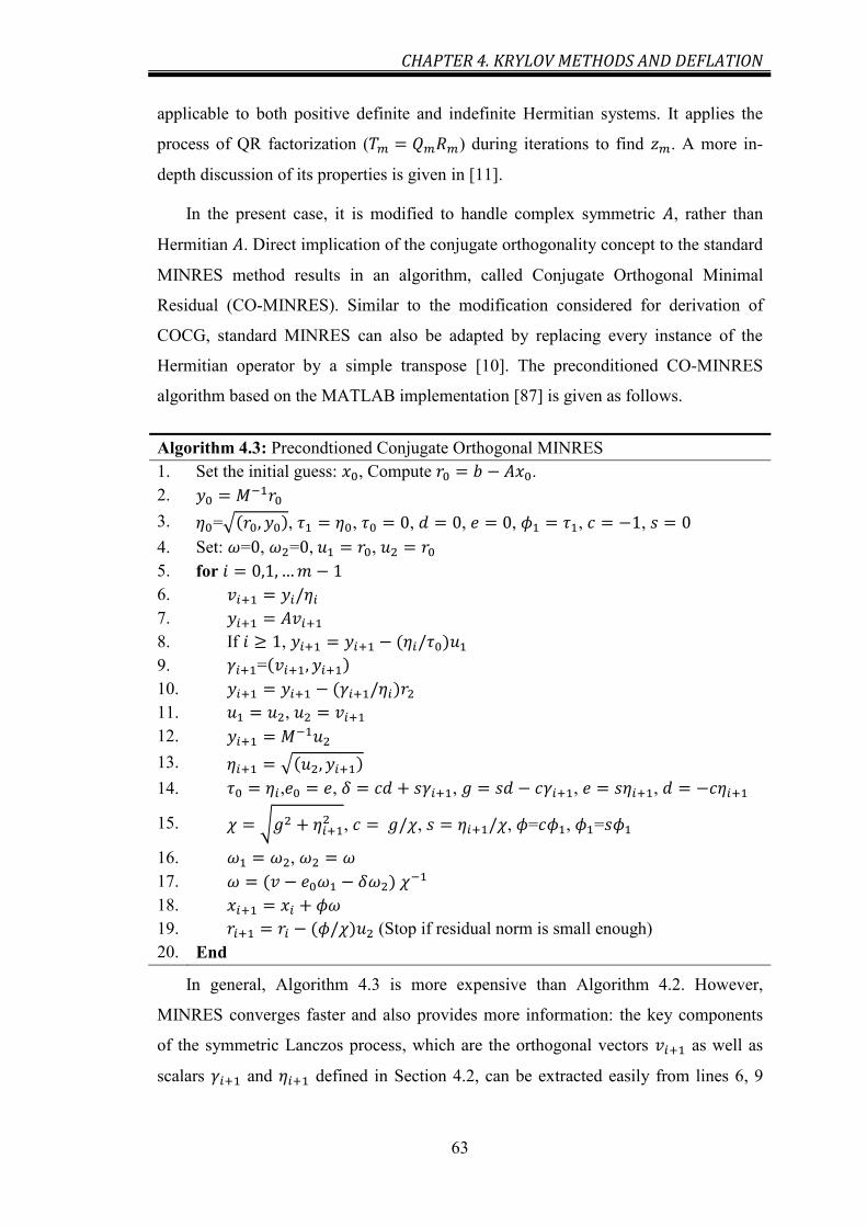
CHAPTER 4. KRYLOV METHODS AND DEFLATION
63
applicable to both positive definite and indefinite Hermitian systems. It applies the
process of QR factorization ( ) during iterations to find . A more in-
depth discussion of its properties is given in [11].
In the present case, it is modified to handle complex symmetric , rather than
Hermitian . Direct implication of the conjugate orthogonality concept to the standard
MINRES method results in an algorithm, called Conjugate Orthogonal Minimal
Residual (CO-MINRES). Similar to the modification considered for derivation of
COCG, standard MINRES can also be adapted by replacing every instance of the
Hermitian operator by a simple transpose [10]. The preconditioned CO-MINRES
algorithm based on the MATLAB implementation [87] is given as follows.
Algorithm 4.3: Precondtioned Conjugate Orthogonal MINRES
1. Set the initial guess: , Compute .
2.
3. =√ , , , , , , ,
4. Set: = , = , ,
5. for
6.
7.
8. If ,
9. =
10.
11. ,
12.
13. √
14. , , , , ,
15. √ , , , = , =
16. ,
17.
18.
19. (Stop if residual norm is small enough)
20. End
In general, Algorithm 4.3 is more expensive than Algorithm 4.2. However,
MINRES converges faster and also provides more information: the key components
of the symmetric Lanczos process, which are the orthogonal vectors as well as
scalars and defined in Section 4.2, can be extracted easily from lines 6, 9

CHAPTER 4. KRYLOV METHODS AND DEFLATION
64
and 13 of the above algorithm. These provide information about the coefficient matrix
and can be used in modified Krylov methods (explained in Section 4.4).
4.3 Generalized Minimal Residual, GMRES
The Generalized Minimal Residual (GMRES) method is an iterative method for
general non-symmetric matrices (and preconditioners), which minimizes the residual
norm over the Krylov subspace. The method is based on the Arnoldi approach [15] for
full orthogonalization and is given as follows:
Algorithm 4.4: Generalized Minimal Residual (GMRES)
1. Set the initial guess: , Compute
2. Set ‖ ‖ and
3. for
4.
5. for
6. ⟨ ⟩,
7. End
8. ‖ ‖
9.
10. End
11. Compute , the minimizer of ‖ ‖ and
12. End
Lines 1 to 10 of the above algorithm are Arnoldi iterations for creating a fully
orthogonal subspace, in which every new vector is orthogonalized to the all
previous vectors in . The approximate solution in GMRES is then obtained by
computing the vector by a sophisticated version of the QR decomposition of the
matrix , such that the 2 norm of the residual is minimized over
. See [85] for a preconditioned version of GMRES.
Although the GMRES method has a good convergence performance, it requires
storing the entire sequence of vectors and the memory requirement increases as the
number of iterations increases. If the iteration number is large, the GMRES
algorithm becomes impractical because of memory and computational requirements.
To remedy this problem, the algorithm can be restarted. The restarted GMRES
follows the idea of the original GMRES, except that after some steps, the algorithm is
repeated by a new initial guess.

CHAPTER 4. KRYLOV METHODS AND DEFLATION
65
4.4 Krylov Deflation
Incorporation of a good preconditioner is one of the most widely used approaches
to accelerate the speed of convergence for Krylov methods. By applying the
preconditioner, the spectrum of is modified with the general goal of obtaining a
matrix that is close to the identity matrix. In this section, we consider an approach for
convergence acceleration that is different from preconditioning, called deflation. Here
the search space of the Krylov subspace method is enlarged by a suitably chosen
subspace that contains useful information about the system that is not adequately
addressed by the action of the preconditioner.
The need for deflation comes from the fact that the convergence of any Krylov
subspace method is affected by the spectrum of the matrix , especially the largest
and smallest eigenvalues. It is clear that CG methods converge more slowly for a
matrix that has small eigenvalues, even after applying a preconditioner.
The Multilevel/ASP/AMG preconditioning cycles described in the previous
chapter try to capture error components related to the highest and lowest eigenvalues
successively, by construction of a multilevel hierarchy. This hierarchy was defined by
transfer operators between the higher order levels and continued with virtual grid
transfer operators below the Whitney level. The cycle aims to transfer error parts
invariant to the relaxation to the next lowest (coarser) level. Errors that remain after
the smoother has been applied and that must be reduced at the next level are called
“algebraically smooth”. Algebraically smooth components belong to the space of
eigenvectors of that have small eigenvalues and for rapid convergence, accurate
representation of them on the coarser level is needed. The nature of the algebraically
smooth errors and the near null space of affect the performance of the
preconditioned Krylov solver and degrade the convergence.
A frequently effective remedy for slow convergence is to directly deflate the
troublesome eigenvalues (eigenvectors) from the problem. This can be done with
construction of an auxiliary approximation subspace that is specifically designed to
target the problematic modes. Numerous techniques can be used to remove the
problematic eigenvectors. Here, the deflated Krylov approach is used. The goal of
deflated Krylov is to remove from the system the eigenspace corresponding to
troublesome, algebraically smooth, eigenvectors. As will be shown, it permits the

CHAPTER 4. KRYLOV METHODS AND DEFLATION
66
incorporation of existing knowledge about the space of troublesome eigenvectors
available from a previous calculation, or a nearby problem.
Deflation is often used for solving one particular matrix with multiple right-hand
sides vectors. The idea then is to use information from the solution of the first right-
hand side to assist subsequent right-hand sides. Here, the deflation idea is tailored
specifically to solving a sequence of problems, , which are generated during
the p-adaption process. In the next section, a framework on how COCG and CO-
MINRES can be improved based on previously-obtained information is described.
After that, the case of solving progressively enlarged system of equations during p-
adaption is considered.
4.4.1 A Framework for Deflated Krylov Methods
In this section, we describe a general framework for deflation of iterative methods
based on the Lanczos process, which simultaneously covers implementations of
several robust Krylov subspace methods. Krylov deflation is in fact a generalization
of the aforementioned basic techniques, that in some instances greatly extends their
efficiency and robustness. It appeared for the first time in the paper of Nicolaides [88]
and a comparable approach was then proposed in [4] and [5]. These techniques glean
“important” information from past problems to enrich the subspace.
Let be the Cholesky factorization of the applied preconditioner in line 7
of preconditioned COCG or line 12 of preconditioned CO-MINRES. Here, we assume
that the columns of a matrix are the “deflation vectors” that approximately span the
space of slow converging modes of the preconditioned system , where
, and . The deflated Lanczos algorithm [88] starts
with an initial vector ‖ ‖ orthogonal to and builds a sequence of vectors
such that [4]:
; ‖ ‖ (4.36)
The subspace [ ] can be obtained by applying the standard Lanczos
procedure to the auxiliary matrix
(4.37)

CHAPTER 4. KRYLOV METHODS AND DEFLATION
67
where ( )
. If the matrix is singular, its pseudo-inverse is
considered. To satisfy , the residual vector should be associated
with a special initial guess
( ) (4.38)
for some arbitrary . The resulting Krylov subspace at the th step is denoted by
( ) and the algorithm seeks an approximate solution
( ) by requiring that the residual be orthogonal to ( ).
Therefore, the change to the standard symmetric Lanczos algorithm is minimal and
can be summarized as follow:
- Based on a given , pre-compute ( )
and the initial
approximation vector using (4.38).
- Construct a symmetric Lanczos space based on the coefficient matrix instead
of by modifying all the matrix-vector products as follows:
(4.39)
As with the standard Lanczos algorithm, the scalar computed during the process
can be stored in a tridiagonal matrix, , and the resulting vectors satisfy
. The difference here is that since the solution is approximated in the space
generated by and , the inclusion is beneficial in accelerating the convergence,
even when contains only poor approximations of slow-converging eigenvectors.
4.4.2 Preconditioned Deflated COCG
Putting relations (4.36) to (4.39) together and following the similar approach for
derivation of standard COCG algorithm, the deflated version of COCG that satisfies
all the recurrence relations can be obtained as follows [4]. The main difference in
iterations of preconditioned deflated COCG comparing to COCG is that, the regular
update of the descent direction vector is changed to
, where is the preconditioned residual vector. The algorithm
is as follows:

CHAPTER 4. KRYLOV METHODS AND DEFLATION
68
Algorithm 4.5: Preconditioned Deflated COCG
1. Set the initial guess: . Compute
2. Define deflation subspace [ ] and also pre-compute
3. Set starting vector: . Compute
4. ,
5. for
6. ⁄
7.
8. (Stop if accurate enough)
9.
10. ⁄
11.
12. End
In Deflated COCG, we must store and in addition to the usual vectors of
COCG, which means an additional storage. Deflated-COCG also requires extra
multiplications for pre-computing and calculation of at each step.
However, the cost is much less than that of the preconditioning and the gain in
decreasing the number of iterations makes it well worthwhile in general.
4.4.3 Preconditioned Deflated CO-MINRES
The CO-MINRES algorithm can also be modified by inclusion of the
subspace. The preconditioned deflated version of this Krylov method is given next, in
which modifications to Algorithm 4.3 occur on lines 2, 3 and 20.
Algorithm 4.6: Preconditioend Deflated CO-MINRES
1. Set the initial guess: . Compute
2. Define deflation subspace [ ] and also pre-compute
3. Set starting vector: . Compute
4.
5. =√ , , , , , , ,
6. Set: = , = , ,
7. for
8.
9.
10. If ,
11. =

CHAPTER 4. KRYLOV METHODS AND DEFLATION
69
12.
13. ,
14.
15. √
16. , , , , ,
17. √ , , , = , =
18. ,
19.
20.
21. (Stop if residual norm is small enough)
22. End
4.5 Eigenvector Estimation
As observed in the algorithms for the deflated Krylov solver, the number of
desired eigenvectors must be chosen, along with the eigenvalues to be targeted. In
particular, small eigenvalues related to the near-null space are the most important ones
for accelerating the convergence. There are several distinct ways to find approximate
eigenvectors that are inadequately clustered by the preconditioner and thus, contribute
to poor convergence [4] [5] [89] [90]. One approach is to find pairs such that
the vector ( ) is minimized. Different projection techniques can be applied
for the minimization [90]. This approach however requires additional costs in advance
for identifying the eigenvalues of that are problematic for convergence.
A better approach is to get the Ritz vectors by solving a previous and slightly
different system [89]. The hierarchical nature of the sequence of linear systems
generated by p-adaption suggests that there are similarities between the
systems. For any higher order system, a considerable portion of the matrix and right-
hand side vector are exactly the same as they are for the previous system. In fact, by
increasing the orders from step to , we can assume that the bulk of the solution
vector also remains roughly as it was at step and mainly higher frequency
variations are represented by the newly added unknowns.
From the above reasoning, we assume that deflation information about the
adaptive system can be obtained during the solution of the problem at the first
adaptive step, when all elements are at their lowest order ( ), and not from a
prior knowledge about the problem. For this first step, the solution is obtained by a

CHAPTER 4. KRYLOV METHODS AND DEFLATION
70
CO-MINRES Krylov subspace solver because this preserves better the orthogonality
of the Ritz vectors. Determination of approximate eigenvalues to be applied to
subsequent adaptive steps is achieved by the following harmonic projection
method [4] [89].
Given subspace and tridiagonal matrix from the CO-MINRES iterations,
the method computes eigenpairs by solving the generalized eigenproblem
(4.40)
where
(4.41)
(4.42)
Defining [ ], the problematic modes are expressed in the form
. Equation (4.40) can be solved at a low cost by any technique for dense
generalized eigenvalue problems. For the results in this thesis, the QZ algorithm in
Matlab [87] is used.
4.6 Deflated Krylov for -Adaption
Consider now the matrix equation at the th adaptive step, ,
with unknowns. Each matrix is of the form (3.3), with the same upper left block
. For , the equation can be solved by deflated COCG with deflation vectors
obtained from as follows:
[
]
(4.43)
In summary, the procedure for solving -type hierarchical systems using a
deflated preconditioned Krylov solver is as follows:
- First-order solution: Set = and apply iterations of CO-MINRES,
preconditioned with an appropriate preconditioner (like the ASP/AMG
algorithm described in Chapter 3), to solve . This computes the matrix
that has the Lanczos vectors, and the tridiagonal matrix .
- Select , the number of eigenvectors to be used.

CHAPTER 4. KRYLOV METHODS AND DEFLATION
71
- Eigenvector computation: Find and using (4.41) and (4.42). Solve (4.40)
for eigenvalues and let be the matrix containing the corresponding vectors.
Set and compute
.
- Adaption iterations (Algorithm 4.7): for
Initialize and then transfer into it values from previous solution, with
appropriate indexing.
Set according to (4.43).
Solve by preconditioned deflated COCG with and from initial
guess .
From (4.43) we observe that the computational cost of deflation at every iteration
is limited to finding just the first values of and then multiplying by
. Algorithm 4.7 presents the efficient way of solving adaptive iteration for
in which line 7 to 9 are the required modifications related to deflation for every
iteration.
Algorithm 4.7: Preconditioned Deflated COCG for p-adaption system
1. Initialize from previous adaption step, Compute
2. Define deflation subspace [ ] and also pre-compute
3. Set and , modify: [ ] [ ]
[ ]. Compute
,
4. for
5.
6. If ⁄
7. for
8. [ ] [ ] [ ]
9. End
10.
11. ⁄
12.
13. (Stop if accurate enough)
14. End

CHAPTER 5
Numerical Studies
This chapter demonstrates the performance of the Multilevel/Algebraic Multigrid
approach through some numerical examples of practical interest. We also study the
performance of Krylov subspace solvers equipped with deflation acceleration. The
reference methods for comparison of the current approach are first introduced in
Section 5.1. Next, in Section 5.2 numerical results for the electric field wave problems
are presented. The results for problems involving the quasi-static magnetic field are
given in Section 5.3.
5.1 The Methods Tested
In order to demonstrate the performance of the proposed approach, several
numerical experiments are considered. In each experiment, we adaptively increase the
order of the elements and solve the matrix problem at each adaptive step by either
COCG, CO-MINRES or GMRES, preconditioned with variants of the ASP
preconditioner described in Chapter 3. Depending on the method used for
approximating the solution to the lowest-level system, , the preconditioners
tested are:

CHAPTER 5. NUMERICAL STUDIES
73
- pMUS[ASP(V)] and pMUS[ASP(W)]: The proposed new methods, i.e., pMUS
(Algorithm 3.8) and ASP correction with V-Cycle AMG (Algorithm 3.4) or the
W-cycle AMG (Algorithm 3.5) [97] [98] [99].
- pMUS[A-V]: The lowest-level system is solved by one backward GS step
followed by one forward GS step, both applied to the vector-scalar potential (A-
V) version of the Whitney system, in compact form [13] [92] [97]. This amounts
to a SSOR preconditioner applied to the A-V version of the entire matrix. This
conventional method can be regarded simply as a variant of the V-cycle of
Algorithm 3.8 combined with a version of Algorithm 3.4 in which the projection
onto (line 3) is omitted and the approximate inverse is just another
application of the SSOR preconditioner.
- pMUS[SSOR]: Conventional pMUS with SSOR preconditioning at the lowest
level. This is equivalent to Algorithm 3.8 combined with a version of Algorithm
3.4 in which the projections onto both and are omitted (line 2 to line 4). It is
also equivalent to direct application of the SSOR preconditioner (1.13) to the
entire matrix.
- pMUS[ILU]: Sparse incomplete factorization of [15]. See Section 1.3.3.
- pMUS[LU]: Complete LU factorization of using UMFPACK [7], which is the
conventional pMUS approach (Algorithm 3.2).
The Krylov iterations are terminated when the infinity norm of the residual is
reduced by a factor of . For the examples presented below, the value for this
parameter is set to , unless otherwise stated. For all calculations, double precision
arithmetic is used. Simulations are done using Matlab [87] and performed on a PC
with a -bit, 4-core, Intel GHz processor and GB of RAM. The geometries
are modeled and meshed with ElecNet [91].
5.2 Numerical Results for Wave Problems
For this section, three different kinds of test problem are used. The first involves
closed domains excited with an incoming waveguide mode in order to find an
parameter. The second kind concerns plane-wave scattering by metallic structures in
free space. Finally, free space scattering form complex objects with composite
materials are presented.

CHAPTER 5. NUMERICAL STUDIES
74
5.2.1 Waveguide Cavity Filter: Illustration of the spectrum of the first order
system and sensitivity to mesh refinement
The waveguide cavity filter studied in [3] and [94] is analyzed. The dimension of
the filter shown in Figure 5.1 is , where is the free space
wavelength at 5.86 GHz. At the excitation port, the dominant waveguide mode
is incident. Outgoing waveguide modes are absorbed at the other port. The structure is
discretized with tetrahedral elements and simulations are performed with varying
element sizes, resulting in discretizations with 18,236 elements in the coarsest mesh to
853,868 elements in the finest mesh.
Figure 5.1: Waveguide cavity filter.
Initially, we consider the effects of the spectral properties of the indefinite curl-
curl operator at the lowest level on the convergence behavior of the COCG solver.
Figure 5.2(a) shows the spectrum of the SSOR-preconditioned matrix
at GHz, with a matrix dimension 24,285. It can be seen
that the range of eigenvalues covers both the positive and negative sections of the real
axis. As explained in Section 3.2, in addition to the Type A [93] [14] [93] negative
eigenvalues related to the null space of the curl operator and associated with
unphysical modes, there are Type B negative eigenvalues related to physical
resonances. More of the Type B eigenvalues will become negative as increases.
This can lead to a very large condition number for the discrete problem and poor
convergence of iterative solvers. With this preconditioner COCG converged in 497
iterations.
In Figure 5.2(b), the spectrum of the SSOR-preconditioned A-V system is shown.
From the displaced eigenvalue distribution, it is apparent that many of the negative
eigenvalues, presumably Type A, can be removed by incorporation of the mapping to

CHAPTER 5. NUMERICAL STUDIES
75
Figure 5.2: Eigenvalue spectrum for preconditioned matrix of cavity filter,
(a) SSOR, (b) A-V SSOR.
the scalar space, . For this better conditioned system, the COCG solver converged in
173 iterations. However, we see that there are still eigenvalues close to zero, both
positive and negative, and this leads to the degradation of the Krylov solver
performance.
Finally, the results of employing the additive ASP preconditioner (Algorithm
3.3 with 1 level AMG approximation, ) are illustrated in Figure 5.3(a) and (b),
for the undamped ( ) and damped ( ) matrix (3.45), respectively. The first
point to notice is the strong clustering around 1 in Figure 5.3(b). Even better, by
introducing the complex shift factor, the negative imaginary half plane of the
spectrum is mapped to a roughly circular pattern in the right half plane. The COCG
iteration counts for the undamped and damped systems are 97 and 43, respectively.
We see that the preconditioned system with more eigenvalues shifted away from the
origin and located in the right-hand half of the complex plane can be solved much
more efficiently with the Krylov solver.
Table 5.1 compares the corresponding iterations and CPU times required for
COCG preconditioned with SSOR, A-V and ASP methods with varying mesh size.
For ASP, the value of is taken as 1.5 and the AMG levels are increased from 1 to 3
through the refinement, to avoid the direct solution of a matrix with dimension larger

CHAPTER 5. NUMERICAL STUDIES
76
Figure 5.3: Eigenvalue spectrum for preconditioned system of cavity filter,
(a) ASP with , (b) ASP with .
than 8,000. The convergence of ASP in additive and multiplicative versions is
superior to the other methods, and the performance is least sensitive to the mesh
refinement parameter . In fact, the ASP-preconditioned systems converge in a
number of iterations that is independent of the mesh size. Among the different
versions of the ASP preconditioner, the W-cycle gives the lowest number of
iterations, with roughly same CPU time as the V-cycle, and in the following tests just
the results with are given. In Figure 5.4, it is shown how the iteration counts and
CPU time of the preconditioned COCG increase as the total number of unknowns and
Table 5.1: Comparison of number of iterations and CPU time (s) for the waveguide cavity filter
at 5.86 GHz.
Number of unknowns ( ) 24,285 57,487 121,203 220,753 502,073 1,043,207
Number of non-zeros ( ) 263,840 750,549 1,598,916 4,034,374 9,935,252 27,914,831
⁄ 0.192 0.113 0.069 0.049 0.043 0.031
SSOR
Iteration 467 827 1256 1267 1977 2202
CPU Time 5.58 29.96 98.15 263.95 1109.4 3,609.8
A-V SSOR
Iteration 128 168 242 296 376 497
CPU Time 2.11 7.98 24.70 81.20 270.04 1029.31
1 Level AMG 2 Level AMG 3 Level AMG
ASP-
Setup Time 0.37 1.41 1.86 4.25 9.75 25.55
Iteration 62 67 63 65 69 69
CPU Time 1.63 5.67 9.49 24.51 67.45 192.16
ASP-
Iteration 46 47 46 50 49 48
CPU Time 1.20 4.11 8.32 22.33 56.25 155.92
ASP-
Iteration 26 26 23 25 24 24
CPU Time 1.64 4.32 9.12 24.79 62.39 177.81

CHAPTER 5. NUMERICAL STUDIES
77
nonzeros entries of is varied by increasing the number of tetrahedra. From the
ASP curve, the computational complexity is , where is the number of
nonzeros in . By contrast, the complexity of A-V is . The computed
scattering parameter versus the frequency of excitation is shown in Figure 5.5 and
demonstrates very good agreement with reported results in [94].
Figure 5.4: Variation of number of iterations and CPU time for waveguide cavity filter.
Figure 5.5: Absolute value of for waveguide cavity filter. Reference results are taken from [94].
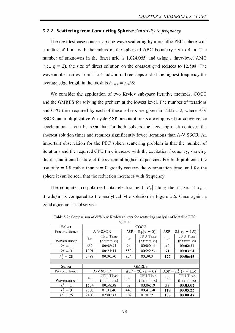
CHAPTER 5. NUMERICAL STUDIES
78
5.2.2 Scattering from Conducting Sphere: Sensitivity to frequency
The next test case concerns plane-wave scattering by a metallic PEC sphere with
a radius of 1 m, with the radius of the spherical ABC boundary set to 4 m. The
number of unknowns in the finest grid is 1,024,065, and using a three-level AMG
(i.e., ), the size of direct solution on the coarsest grid reduces to 12,508. The
wavenumber varies from 1 to 5 rads/m in three steps and at the highest frequency the
average edge length in the mesh is ;
We consider the application of two Krylov subspace iterative methods, COCG
and the GMRES for solving the problem at the lowest level. The number of iterations
and CPU time required by each of these solvers are given in Table 5.2, where A-V
SSOR and multiplicative W-cycle ASP preconditioners are employed for convergence
acceleration. It can be seen that for both solvers the new approach achieves the
shortest solution times and requires significantly fewer iterations than A-V SSOR. An
important observation for the PEC sphere scattering problem is that the number of
iterations and the required CPU time increase with the excitation frequency, showing
the ill-conditioned nature of the system at higher frequencies. For both problems, the
use of rather than greatly reduces the computation time, and for the
sphere it can be seen that the reduction increases with frequency.
The computed co-polarized total electric field | | along the axis at
is compared to the analytical Mie solution in Figure 5.6. Once again, a
good agreement is observed.
Table 5.2: Comparison of different Krylov solvers for scattering analysis of Metallic PEC
sphere.
Solver COCG
Preconditioner A-V SSOR
Iter.
CPU Time
(hh:mm:ss) Iter.
CPU Time
(hh:mm:ss) Iter.
CPU Time
(hh:mm:ss) Wavenumber
680 00:08:34 96 00:05:14 40 00:02:21
1991 00:24:44 552 00:25:23 71 00:03:54
2483 00:30:50 824 00:30:31 127 00:06:45
Solver GMRES
Preconditioner A-V SSOR
Iter.
CPU Time
(hh:mm:ss) Iter.
CPU Time
(hh:mm:ss) Iter.
CPU Time
(hh:mm:ss) Wavenumber
1534 00:58:38 69 00:06:19 37 00:03:02
2083 01:31:40 443 00:41:50 118 00:05:22
2403 02:00:33 702 01:01:21 175 00:09:48

CHAPTER 5. NUMERICAL STUDIES
79
Figure 5.6: Magnitude of co-polarized electric field along the propagation direction.
5.2.3 Metallic Frequency Selective Surface (FSS): Sensitivity to the damping
parameter
This test problem concerns scattering from a metallic-
grid frequency selective surface (FSS) consisting of rectangular perforations of
varying size on a metallic screen (Figure 5.7), as described in [95]. The geometry is
illuminated with a 10 GHz plane wave. The incident wave is along the axis. The
outer truncation ABC boundary is a rectangular box, which is the same shape as the
target. The distance between the ABC boundary and the target is . Because of
the fine details of this non-periodic scatterer, a large number of elements is needed.
The edge lengths in the mesh range from to , with , and
there are 2,416,388 unknowns. Once again, a three-level multilevel scheme is used to
reduce to 30,932 the size of the matrix to which direct solution is applied.
We consider the effects of the damping parameter on the performance of COCG
Krylov subspace method applied to . The number of iterations and also CPU
Figure 5.7. Metallic frequency selective surface with rectangular perforations.

CHAPTER 5. NUMERICAL STUDIES
80
Table 5.3: Comparison of effects of damping parameter on the
convergence of Krylov solver for metallic FSS problem.
Solver COCG
Iter.
CPU Time
(hh:mm:ss) Preconditioner
A-V SSOR 2384 01:01:22
696 01:08:06
466 00:52:20
249 00:27:41
201 00:21:17
173 00:20:48
178 00:20:51
194 00:21:36
217 00:24:15
278 00:29:50
time for different damping parameters are given in Table 5.3, where multiplicative W-
cycle ASP preconditioners and A-V SSOR are employed for convergence
acceleration. It can be seen that the use of for shifted Laplacian
preconditioner achieves the shortest solution times and requires significantly fewer
iterations than A-V SSOR. Figure 5.8 demonstrates the convergence behavior of the
preconditioned system. Clearly, the iterative solvers preconditioned with ASP exhibit
a robust and fast convergence for the first order problem. The computed electric field
over the plane, 0.5 cm from the scatterer, is shown in Figure 5.9.
Figure 5.8: Convergence history of preconditioned Krylov solver for FSS scattering analysis.
Figure 5.9: Scattering from metallic FSS; magnitude of the electric field. (a) Ex, (b) Ey, (c) Ez.

CHAPTER 5. NUMERICAL STUDIES
81
5.2.4 SRR Loaded rectangular Waveguide: p-adaption and deflation
The next example is a rectangular metallic waveguide loaded with split ring
resonators (SRRs). This configuration has attracted extensive attention [100] [101],
since it provides the realization of negative index metamaterials and novel methods to
miniaturize waveguide-based devices. The geometry is directly taken from [100],
proposed for the creation of a stopband above the ordinary waveguide cutoff
frequency. The geometry, showing the excitation port A and absorption port B, is
presented in Figure 5.10.
SRR elements can be found in [100], noting that printed elements on the middle
and left lateral wall slabs are a factor of smaller than the elements on the right
(a)
(b)
(c)
Figure 5.10: (a) The geometry of SRR loaded waveguide filter along with the excitation and absorption
ports. (b) The mesh discretization. (c) Intensity distribution of electric field strength within the loaded
waveguide.
Po
rt A
Po
rt B
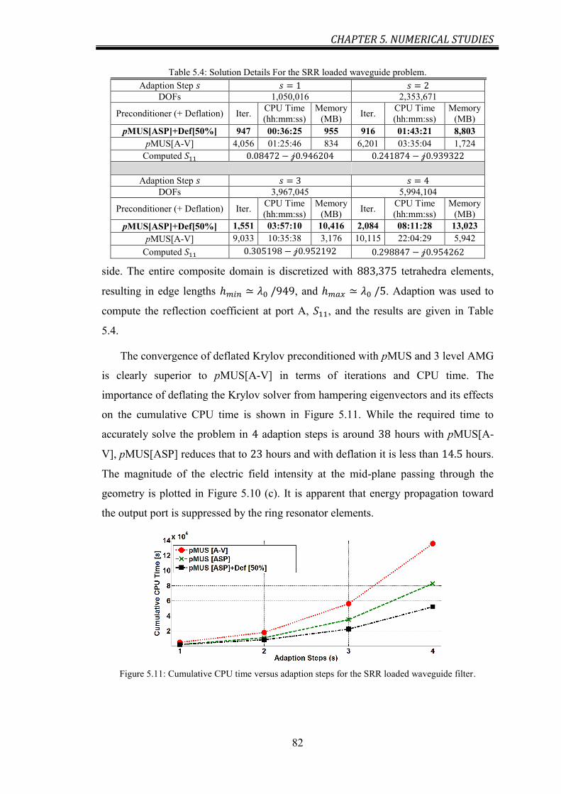
CHAPTER 5. NUMERICAL STUDIES
82
Table 5.4: Solution Details For the SRR loaded waveguide problem.
Adaption Step
DOFs 1,050,016 2,353,671
Preconditioner (+ Deflation) Iter. CPU Time
(hh:mm:ss)
Memory
(MB) Iter.
CPU Time
(hh:mm:ss)
Memory
(MB)
pMUS[ASP]+Def[50%] 947 00:36:25 955 916 01:43:21 8,803
pMUS[A-V] 4,056 01:25:46 834 6,201 03:35:04 1,724
Computed
Adaption Step
DOFs 3,967,045 5,994,104
Preconditioner (+ Deflation) Iter. CPU Time
(hh:mm:ss)
Memory
(MB) Iter.
CPU Time
(hh:mm:ss)
Memory
(MB)
pMUS[ASP]+Def[50%] 1,551 03:57:10 10,416 2,084 08:11:28 13,023
pMUS[A-V] 9,033 10:35:38 3,176 10,115 22:04:29 5,942
Computed
side. The entire composite domain is discretized with tetrahedra elements,
resulting in edge lengths , and . Adaption was used to
compute the reflection coefficient at port A, , and the results are given in Table
5.4.
The convergence of deflated Krylov preconditioned with pMUS and 3 level AMG
is clearly superior to pMUS[A-V] in terms of iterations and CPU time. The
importance of deflating the Krylov solver from hampering eigenvectors and its effects
on the cumulative CPU time is shown in Figure 5.11. While the required time to
accurately solve the problem in adaption steps is around hours with pMUS[A-
V], pMUS[ASP] reduces that to hours and with deflation it is less than hours.
The magnitude of the electric field intensity at the mid-plane passing through the
geometry is plotted in Figure 5.10 (c). It is apparent that energy propagation toward
the output port is suppressed by the ring resonator elements.
Figure 5.11: Cumulative CPU time versus adaption steps for the SRR loaded waveguide filter.

CHAPTER 5. NUMERICAL STUDIES
83
5.2.5 Conducting Sphere Surrounded by 60-Node Buckyball: Sensitivity to
the size of the deflation subspace
This test case concerns free space scattering from a conducting sphere surrounded
by a polyhedral, 60-node “buckyball”, acting as a metallic frame to reduce the
backscattered wave from the sphere at MHz [102]. The problem is shown in
Figure 5.12. The diameter of the internal solid sphere is m and the external
polyhedral conducting frame has diameter of m with an edge width and thickness
of m and m, respectively. An ABC is applied over a spherical
surface m away from the buckyball. The mesh obtained after discretization consists
of nodes and elements with minimum and maximum edge lengths
of and , respectively. In this computation, the number of
unknowns increases from to in adaptive steps.
Figure 5.12: Geometry of 6 m metal sphere surrounded with a 10m spherical polyhedral frame.
The detailed computational information is listed in Table 5.5. For pMUS[ASP], 3
AMG levels are used, with , and DOFs, respectively.
Table 5.5: Solution Details For the buckyball scattering problem.
Adaption Step
DOFs 810,595 2,319,586
Preconditioner (+ Deflation) Iter. CPU Time
(hh:mm:ss)
Memory
(MB) Iter.
CPU Time
(hh:mm:ss)
Memory
(MB)
pMUS[ASP]+Def[50%] 108 00:03:58 928 124 00:08:39 2,635
pMUS[A-V] 2,058 00:21:10 686 2,173 01:19:52 1,767
Adaption Step
DOFs 3,716,547 5,710,953
Preconditioner (+ Deflation) Iter. CPU Time
(hh:mm:ss)
Memory
(MB) Iter.
CPU Time
(hh:mm:ss)
Memory
(MB)
pMUS[ASP]+Def[50%] 130 00:12:50 3,621 157 00:25:30 5,895
pMUS[A-V] 2,138 02:18:15 2,673 2,188 04:19:25 4,908

CHAPTER 5. NUMERICAL STUDIES
84
As indicated in the table, the run time required by pMUS[ASP] with 57 deflation
vectors (50%) is much less than with pMUS[A-V] at each adaption step.
Next we consider the effect of varying the dimension, , of the deflation subspace
from 0 (no deflation) to ( deflation). Figures 5.13 (a-c) compare the
number of iterations, computation time and memory usage for several choices of .
Increasing leads to fewer iterations, but at the cost of more memory usage. We also
see that increasing beyond about 50% does not bring much further reduction in
computation time. Towards the end of the adaption, deflation leads to a
reduction in cumulative computation time and a reduction in Krylov iterations.
Figure 5.13: Comparison of effects of deflation on: (a) Krylov iterations, (b) CPU time and (c) memory
usage, for the buckyball problem.

CHAPTER 5. NUMERICAL STUDIES
85
5.2.3 Jerusalem Cross Screens FSS: Illustration of matrix dimensions in
multilevel hierarchy
For the final experiment related to wave problems, results obtained from the
scattering analysis of a finite, noncommensurate, frequency selective surface (FSS)
are presented. The device, shown in Figure 5.14, consists of two dissimilar Jerusalem
cross screens (dimensions taken from [103]) printed on opposite sides of a
dielectric slab, where is the free space wavelength at 3 GHz.
The dielectric relative permittivity is . Such composite and multi-
layer structures with different periodicities are difficult to handle rigorously using
periodic boundary conditions [103] [104] and analysis of the entire system is usually
needed.
For the computational domain truncation, the geometry is enclosed in a box at
least away from any point on the FSS and the ABC is applied. The structure is
illuminated normally ( direction) with an -polarized plane wave. The mesh
consists of tetrahedra. As observed in Figure 5.14, the mesh is highly
nonuniform, with an average element size of and sizes ranging from
around the metallic regions to near the truncation boundary.
Figure 5.14: Geometry of a Jerusalem cross noncommenserate FSS
(a) Side view. (b) Top view showing the 7 7 upper screen.
(c) Bottom view showing the 5 5 lower screen.

CHAPTER 5. NUMERICAL STUDIES
86
Table 5.6: Solution details for the noncommenserate FSS scattering problem.
DOFs Nonzeros Iter. CPU Time
(hh:mm:ss)
Memory
(MB)
1 2,261,319 36,824,307 533 00:54:28 2,314
2 5,482,526 188,871,828 626 02:07:01 11,241
3 8,909,294 370,550,000 683 03:18:42 14,347
4 12,264,629 626,152,411 594 03:45:56 17,424
A summary of computational statistics for 4 steps of p-adaption, using
pMUS[ASP]+Def[50%], is given in Table 5.6 ( ). In this case pMUS[A-V]
failed at each adaptive step to reduce the residual by a factor of after
iterations. The column labeled “Nonzeros” gives the number of nonzero entries in the
matrix. Note that the matrices become denser as the adaption proceeds, which is
characteristic of p-adaption. Here, as in the previous examples, the number of
iterations is relatively stable, despite the growth in the size of the matrix. At step 4, a
complex valued system with almost million unknowns and billion nonzeros
is solved on a PC in reasonable time.
Table 5.7 gives, for the matrix (4th
adaptive step), the matrices used in its
preconditioner. Since there are some 4th
order elements present at this step, the largest
matrix is (which is just itself). Four levels of AMG are used (i.e., ), so
the smallest matrix is .
The residual history in solving the system is shown in Figure 5.15. Removing
the accelerations provided by deflation results in an increase of and in
Krylov iterations and run time respectively, as well as reduction in memory
usage. Figure 5.16 shows the computed electric field over two cross-sections, both
passing through the center of the structure.
Table 5.7: Matrix Hierarchy Details For the noncommenserate
FSS scattering problem at the 4th adaption step.
Matrix DOFs Nonzeros
12,264,629 626,152,411
12,051,413 525,271,225
10,794,234 416,843,750
2,261,319 36,824,307
259,089 3,487,890
90,448 1,236,772
34,162 480,396
20,174 287,358

CHAPTER 5. NUMERICAL STUDIES
87
Figure 5.15: Residual history of (deflated) preconditioned COCG method
for the noncommenserate FSS scattering at 4th adaption step.
(a)
(b)
Figure 5.16: Visualization of electric field for the noncommenserate FSS
(a) over plane . (b) over plane .
5.3 Numerical Results for the Quasi-static Magnetic Field
Problems
In this section, numerical results related to quasi-static magnetic field problems
are presented. The performance of the current method (pMUS and ASP approach
introduced in Section 3.6) is compared to a standard preconditioner for three
examples.

CHAPTER 5. NUMERICAL STUDIES
88
5.3.3 Shielding Inside a Metallic Cube: V cycle vs. W cycle
For the first example, a hollow, conducting cube placed in a uniform field is
considered. The geometry and the mesh are shown in Figure 5.17. The permeability
and the conductivity of the conductor are and
respectively. The skin depth at the excitation frequency, , is .
The length of the cube is and the wall thickness is . The computational
domain, , is a cube of side . The scalar potential is constrained on two opposite
surfaces of to produce a magnetic field, , that would be uniform in the absence
of the conducting cube. The domain is discretized with tetrahedra,
resulting in scalar and vector unknowns at the lowest order.
Three steps of p-adaption are applied. The matrix problems are solved by the
preconditioned COCG method [86].
Table 5.8 presents the number of unknowns, the number of COCG iterations and
the corresponding CPU times for solving the matrix problem with the accuracy of
at each adaptive step. For the ASP method, scalar AMG employs a
hierarchy of three levels with , and unknowns. The
comparison shows the superior iteration count and run time of ASP at each adaptive
step. The experiments also indicate that a significant improvement can be achieved for
higher order systems if a better algebraic solver, like ASP(W-Cycle), is used at the
first order. The cumulative CPU time for solving the problem with three p-adaptive
steps using pMUS[ASP(W-cycle)] is 3.4 times less than that required by SSOR and
for step 3 the CPU time is 4 times less.
Figure 5.17: Illustration of geometry and discretization for the conducting
cube problem.

CHAPTER 5. NUMERICAL STUDIES
89
Table 5.8: Solution Details For the conducting Cube Problem.
Step 1 Step 2 Step 3
Unknowns 2,875,868 8,578,954 13,345,009
Nonzeros 66,707,982 350,799,470 615,703,547
Preconditioner Iter. CPU Time
(hh:mm:ss) Iter.
CPU Time
(hh:mm:ss) Iter.
CPU Time
(hh:mm:ss)
pMUS[SSOR] 608 00:23:49 652 01:41:55 654 03:03:14
pMUS[ILU(0)] 741 00:28:13 685 01:57:35 628 02:51:45
pMUS[ASP(V-Cycle)] 150 00:12:28 205 00:39:09 206 01:08:05
pMUS[ASP(W-Cycle)] 60 00:13:23 88 00:28:19 94 00:45:55
The convergence history of COCG at step 3 is shown in Figure 5.18. It is
observed that while the convergence rates for SSOR and pMUS[ILU(0)] are nearly
the same, pMUS[ASP(W-cycle)] is able to reduce the number of iterations by a factor
of almost . Results for the computed | | over a cross-section and field penetration
inside the conducting cube are shown in Figure 5.19.
Figure 5.18: Convergence history of COCG with different preconditioners
for solving the conducting cube problem at p-adaptive step 3.
Figure 5.19: Variation of the normalized magnetic field strength
| | | |⁄ over a cross section passing through the cube center.

CHAPTER 5. NUMERICAL STUDIES
90
5.3.1 Benchmark TEAM Problem No. 7: Scalability by p-refinement
For the second example, the benchmark TEAM problem no. 7 is
analyzed [105] [106]. It consists of a conducting aluminum plate with a hole, above
which a racetrack coil with a time-harmonic driving current is placed. The aluminum
plate has a conductivity of and the sinusoidal driving current
of the coil is AT. The frequency is . In order to employ the
formulation, the hole is treated as a conductor with very low conductivity
.
The computational domain is restricted to a cube of m edge length with the
boundary condition over its surfaces. For the discretization,
tetrahedra are used and the resulting mesh consists of nodes and
edges. The geometry of the problem (without the surrounding box) and its
discretization in the conducting region can be seen in Figure 5.20 (a). Note that the
mesh is well refined on the surface of the conductor regions.
The problem is analyzed p-adaptively in 6 steps with . In Table 5.9, the
performance of the COCG method for different adaption steps and different
preconditioning algorithms are shown. For the ASP method, 2 level AMG is
employed for approximating the vector nodal systems and the number of unknowns at
the lowest level is . From the experiment, it can be seen that using ASP for the
lowest order correction results in a greatly reduced number of iterations.
(a) (b)
Figure 5.20: (a) Mesh discretization for the TEAM 7 benchmark problem,
(b) Magnetic field ( ) at the cut plane .

CHAPTER 5. NUMERICAL STUDIES
91
Table 5.9: Solution details for the TEAM problem no. 7
Preconditioner PMUS[SSOR] pMUS[ILU(0)]
pMUS
[ASP(W-Cycle)] Speed up
(SSOR/ASP) Step DOFs ( ) Iter.
CPU Time
(hh:mm:ss) Iter.
CPU Time
(hh:mm:ss) Iter.
CPU Time
(hh:mm:ss)
1 623,613 622 00:05:34 480 00:03:42 63 00:01:48 3.1
2 1,526,157 494 00:13:24 494 00:13:50 64 00:03:01 4.3
3 3,050,178 498 00:33:59 495 00:36:30 75 00:06:52 4.8
4 4,592,119 496 01:04:32 475 00:59:38 87 00:11:54 5.4
5 5,624,662 463 01:07:24 468 01:18:15 70 00:12:58 5.6
6 7,014,699 454 01:31:59 487 01:26:34 71 00:16:39 5.8
More significant than the number of iterations is the CPU time. The reduction in
iterations results in fewer time-consuming smoothing steps for the higher order blocks
of the matrix. Figure 5.21 compares the time in minutes to solve the eddy current
problem at each adaption step. Here we see that pMUS[ASP] works very well and is
always faster than SSOR and pMUS[ILU(0)]. The cumulative CPU time for all 6
steps using ASP is more than 5 times less than when using SSOR. For the last 4 points
of the ASP curve, the CPU time grows roughly as . The computed magnetic field
at step 6 over the specified cut plane is displayed in Figure 5.20 (b). The problem has
measured results as well [106]. Figure 5.22 compares the numerical values of the
vertical magnetic flux density with measured values along a pre-defined
line of the TEAM 7 benchmark problem.
Figure 5.21: CPU time versus number of unknowns for different adaption steps of TEAM 7 problem.
Figure 5.22: Computed along a pre-defined line of the TEAM 7 problem ( , ,
and ) compared with measured values.
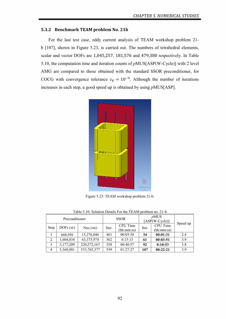
CHAPTER 5. NUMERICAL STUDIES
92
5.3.2 Benchmark TEAM problem No. 21b
For the last test case, eddy current analysis of TEAM workshop problem 21-
b [107], shown in Figure 5.23, is carried out. The numbers of tetrahedral elements,
scalar and vector DOFs are , and respectively. In Table
5.10, the computation time and iteration counts of pMUS[ASP(W-Cycle)] with 2 level
AMG are compared to those obtained with the standard SSOR preconditioner, for
COCG with convergence tolerance . Although the number of iterations
increases in each step, a good speed up is obtained by using pMUS[ASP].
Figure 5.23: TEAM workshop problem 21-b.
Table 5.10: Solution Details For the TEAM problem no. 21-b
Preconditioner SSOR pMUS
[ASP(W-Cycle)] Speed up
Step DOFs ( ) Nnz ( ) Iter. CPU Time
(hh:mm:ss) Iter.
CPU Time
(hh:mm:ss)
1 660,956 15,276,046 461 00:03:38 34 00:01:31 2.4
2 1,604,034 63,375,974 562 0:15:13 61 00:03:51 3.9
3 3,177,209 220,372,167 558 00:40:57 92 0:10:53 3.8
4 5,368,881 533,765,377 559 01:27:27 107 00:22:21 3.9

CHAPTER 6
Conclusions
6.1 Summary
The finite element discretization of the vector curl-curl equation leads to a sparse
and complex-symmetric linear system of equations. In high frequency simulation of
the electric field inside complex structures the linear system is generally large, highly
indefinite and extremely ill-conditioned. These properties make solution of the linear
system a challenging step, especially when direct methods are out of reach.
Application of Krylov iterative methods preconditioned with standard
preconditioners, like SSOR or incomplete LU factorization, does not result in a
satisfactory convergence. Specialized preconditioning techniques are required.
In this thesis, an effective iterative method to solve the discrete curl-curl equation
with p-adaptive finite element analysis has been proposed. The method is a
preconditioned Krylov subspace iteration, with a p-type Multilevel and Algebraic
Multigrid cycle serving as the preconditioner for the block structured system. For the
lowest order system at the bottom of the V-cycle, performance of different correction
approaches has been tested, which are denoted by pMUS[method] in this work.
Effects of different lowest level correction on the convergence rate are shown and

CHAPTER 6. CONCLUSIONS
94
incorporation of a successful ASP/AMG algorithm has been carried out as a
replacement for the commonly used direct solve. The success of the algebraic solver
is in fact based on proper choice of multigrid components with respect to the
characteristics of the underlying PDEs.
The construction of coarsening operators in nodal AMG is based on robust nodal
aggregation algorithms [17] which allows for fast, automated coarse space
construction, without the need to build a hierarchy of nested finite-element meshes.
The coarse grid operators are also created in an algebraic fashion using the Galerkin
coarse grid approximation which allows the coarse sub-problems to be constructed
quickly without discretization. This results in an overall fast setup phase with reduced
time compared to the iteration phase. The performance of the algebraic solver also
depends on the accuracy of nodal AMGs for discrete second-order elliptic equations
and improvements in this area can provide further robustness of the proposed
preconditioning approach.
Extensive numerical experiments have been performed and results are presented
for both wave and quasi-static problems. The test cases used are complicated
problems to solve and the promising numerical results have shown the robustness and
efficiency of the new preconditioner. The well-known A-V SSOR preconditioning
approach is used as an efficient reference method. Krylov methods like COCG, CO-
MINRES and GMRES preconditioned with the current approach were always
considerably faster than A-V for the test problems considered. The performance of
Krylov algorithms is even further enhanced during the p-adaption analysis by
construction of a Deflation sub-space and removing the contribution of smallest
eigenvalues from the preconditioned system.
6.2 Contributions
The main contributions of this thesis are summarized as below:
Application of multilevel Schwarz preconditioning to adaptive FEM systems:
This work extends the solution idea of p-type multilevel Schwarz (pMUS) for
uniform order systems [60] [47] to the linear systems that arise in p-adaption. By a

CHAPTER 6. CONCLUSIONS
95
suitable numbering of the high order DOFs, a block structured matrix is obtained
which can be approximately inverted by a V-cycle, as with conventional pMUS.
Development of an ASP/AMG correction for the wave equation:
I applied the Auxiliary Space Preconditioning approach for Whitney elements,
which was only tested before on quasi-static problems, to wave-scattering
problems. Design of several preconditioning algorithms has been carried out and
development of a fully algebraic correction based on symmetric V-cycle and W-
cycle multigrid approximations has been achieved. The results shows that a
ASP/AMG correction combined with a Krylov iteration is an effective technique
for wave problems that are analyzed with large numbers of Whitney finite
elements. As the mesh density increases, the number of Krylov iterations is
constant and the CPU time grows linearly with the number of matrix nonzeros.
Development of an ASP/AMG correction for the T- method:
An efficient algebraic multigrid algorithm for the solution of quasi-static problems
by the formulation is developed. Similar algebraic methods have been
applied previously to the matrices arising from purely vector formulations, using
Whitney edge elements [23] [74] [75]. However, the method in this thesis is
different in that it works with the method, which involves both scalar and
vector unknowns. For the assembled matrix equation at level one, a partitioning is
considered into vector unknowns (defined over the cotree edges of conductors)
and scalar unknowns (defined over the whole mesh). Corresponding auxiliary
space problems are then constructed for the separate treatment of the error related
to the vector and scalar DOFs. The first order residual in this case is transferred
into five auxiliary space problems: four equivalent nodal problems inside the
conducting regions and one nodal problem for the whole mesh. Corrections are
then connected in symmetric V and W cycles to result in an efficient
preconditioner for the Krylov methods.
Incorporation of the ASP/AMG method for the first order problem into
the pMUS algorithm:
Complete matrix factorization of the lowest level matrix in pMUS is not
applicable to large scale discrete PDEs. Considering the promising performance of
the proposed ASP/AMG approaches for Whitney elements, I combined

CHAPTER 6. CONCLUSIONS
96
corrections of high-order, hierarchical DOFs in pMUS with the new ASP
corrections at level one into a symmetric preconditioner, which allows pMUS to
be applied even when the matrix at lowest order is too big for direct solution. The
algebraic lowest level correction is especially useful for problems with fine
geometric details, requiring a very large mesh in which the bulk of the elements
remain at low order. pMUS with ASP/AMG treatment has shown to be always
faster than pMUS[A-V] and in some cases 10 times faster.
Application of “shifted Laplace” preconditioning to the curl-curl wave
equation:
For wave problems, the ASP/AMG algorithm is tailored to use a modified bilinear
form. This is similar to the “shifted Laplace” technique that was developed for the
scalar Helmholtz equation. Rather than being applied to the original bilinear form,
corrections of the vector nodal part in the algorithm are applied to a shifted
version, which can be thought of as the original operator with a complex
perturbation. This is shown to provide a satisfactory multigrid inverse
approximation and a significant convergence acceleration for the Krylov subspace
methods, because of the improved spectral properties of the preconditioned linear
system.
Development of a deflated Krylov scheme for faster solution of adaptive FEM
systems:
For problems with strong ill-conditioning, some eigenvalues may lie very close to
zero and by proper treatment of these small eigenvalues further acceleration of
Krylov methods can be achieved. The so-called deflation technique is used in this
work to project out smallest eigenvalues from the preconditioned system, such
that their contribution is removed from the residual. Rather than using expensive
eigenvector computation, the construction of the deflation sub-space is, for the
first time, based on an estimation of eigenvectors from information obtained when
solving the first problem in a p-adaptive sequence. Numerical experiments show
that the deflated Krylov solver provides additional reduction in run time time
(20% to 40%), at the expense of a greater memory requirement (10% to 35%).

CHAPTER 6. CONCLUSIONS
97
6.3 Recommendations
Suggestions for future research include:
Parallelization of solver components:
Some parallel implementation of the proposed method would be possible for very
large scale applications. In particular, the correction steps involved in handling
each of the four or five nodal sub-problems in ASP (from the finest grid to the
coarsest grid) are separate and can be executed in parallel. The setup phase and
some steps of the deflated Krylov solvers can also be implemented on a parallel
machine.
Combination with multilevel-based incomplete LU methods
For the current approach, adding more levels in the nodal AMG algorithm can be
continued as long as the virtual AMG meshes can adequately represent field
variations on the scale of the wavelength (for wave problems). If this limit is
exceeded, the preconditioner quality suffers and the Krylov solver takes longer to
converge, or may even fail to converge. Therefore, for problems which are
electrically very large, the coarsest nodal problem may still be too large to
factorize. In this case, one alternative approach for continuing the same algebraic
concept at the bottom of the algorithm is to use a recently proposed inverse-based
multilevel incomplete factorization [108]. In contrast to conventional
methods, the fully algebraic and symmetric multilevel inverse-based
preconditioner may exhibit good efficiency (especially in terms of fill-in) for
solving the coarsest nodal systems by employing a graph partition technique and
reordering into a hierarchical multilevel structure.
Combination with domain decomposition as a local solver
For solving very large and multiscale electromagnetic scattering problems, the
finite element based nonoverlapping domain decomposition methods (DDM) have
been exploited recently that enable each subdomain to be discretized and solved
independently on one processing unit. Of particular interest would be the
combination of the proposed approach with currently developed DDM algorithms.
One may employ the pMUS/ASP algorithm as an effective local solver in every
subdomain. This would allow larger subdomains, which would result in better
performance.
CHAPTER 6. CONCLUSIONS
98
Non-symmetric multigrid components
In this work, I have focused on the complex-symmetric property of the systems in
order to choose multigrid components. Aside from requiring less storage, the
symmetric property of the linear system allows us to use efficient Krylov subspace
algorithms resulting from three term recurrences and based on the specialized
conjugate orthogonality condition. All the preconditioning cycles in this work are
substantially designed to exploit the symmetry in order to maximize the
performance of solvers. However, by using some components that do not use
symmetry, we might be able to develop better multigrid algorithms. For instance,
recently some strategies have been proposed to use a non-symmetric GMRES
smoother as an alternative [109] [110]. Outer iterations related to the Krylov
methods can also be modified by using novel approaches, such as generalized
conjugate residual method [111].

Bibliography
[1] J. F. Lee, D. K. Sun and Z. Cendes, “Full-wave analysis of dielectric waveguides
using tangential vector finite elements,” IEEE Transactions on Microwave Theory
and Techniques, vol. 39, no. 8, pp. 1262-1271, 1991.
[2] J. P. Webb, “Hierarchical vector basis functions of arbitrary order for triangular
and tetrahedral finite elements,” IEEE Transactions on Antennas and
Propagation, vol. 47, no. 8, pp. 1244–1253, 1999.
[3] P. Ingelstrom, “A new set of H(curl)-conforming hierarchical basis functions for
tetrahedral meshes,” IEEE Transactions on Microwave Theory and Techniques,
vol. 54, pp. 106-114, Jan 2006.
[4] Y. Saad, M. Yeung, J. Erhel and F. Guyomarcha, “Deflated Version of the
Conjugate Gradient Algorithm,” SIAM Journal on Scientific Computing. vol. 21,
no. 5, pp. 1909–1926, Apr 2000.
[5] A. M. Abdel-Rehim, R. B. Morgan, D. A. Nicely and W. Wilcox, “Deflated and
Restarted Symmetric Lanczos Methods for Eigenvalues and Linear Equations
With Multiple Right-Hand Sides,” SIAM Journal on Scientific Computing, vol. 32,
no. 1, pp. 129-149, 2010.
[6] T. A. Davis, “Direct Methods for Sparse Linear Systems,” SIAM, Philadelphia,
Part of the SIAM Book Series on the Fundamentals of Algorithms, Sep. 2006
[7] T. A. Davis, “Algorithm 832: UMFPACK, an unsymmetric-pattern multifrontal
method,” ACM Transactions on Mathematical Software, vol. 30, no. 2, pp. 196-
199, June 2004.
[8] T. A. Davis, “UMFPACK User Guide,” Jun, 2012.
[9] P. Tsuji, E. Bjorn, and Y. Lexing, “A sweeping preconditioner for time-harmonic
Maxwell’s equations with finite elements,” Journal of Computational Physics,
vol. 231, no. 9, pp. 3770-3783, 2012.
[10] R. Freund, “Conjugate Gradient-Type Methods for Linear Systems with
Complex Symmetric Coefficient Matrices,” SIAM Journal on Scientific and
Statistical Computing, 1992.
[11] C. C. Paige, and M. A. Saunders, “Solution of sparse indefinite systems of
linear equations,” SIAM Journal on Numerical Analysis, vol. 12, no 4, pp. 617-
629, Sep 1975.
[12] Y. Saad, and M. H. Schultz, “GMRES: A generalized minimal residual
algorithm for solving nonsymmetric linear systems,” SIAM J. Sci. Stat. Comput.,
vol. 7, no. 3, pp. 856-869, Jul 1986.
[13] R. Dyczij-Edlinger, G. Peng and J. F. Lee, “A Fast Vector-Potential Method
Using Tangentially Continuous Vector Finite Elements,” IEEE Transactions on
Microwave Theory and Techniques, vol. 46, pp. 86-868, Jun 1998.
[14] R. Dyczij-Edlinger, G. Peng and J.-F. Lee, “Stability conditions for using
TVFEMs to solve Maxwell equations in the frequency domain,” Int. J. Numer.
Modeling, vol. 13, pp. 245–260, 2000.
[15] Y. Saad, “Iterative Methods for Sparse Linear Systems”, PWS Publishing
Company, 1996, Chapter 10 - Preconditioning Techniques.
[16] M. Bollhofer and Y. Saad, “Multilevel preconditioners constructed from
inverse-based ILUs,” SIAM J. Sci. Comput., vol. 27, no. 5, pp.1627–1650, 2006.
[17] Y. Notay, “An Aggregation-Based Algebraic Multigrid Method,” Electronic
Transactions on Numerical Analysis, vol. 37, pp. 123-146, 2010.

BIBLIOGRAPHY
100
[18] R. Hiptmair, “Multigrid method for Maxwell's equations,” SIAM Journal on
Numerical Analysis, vol. 36, pp. 204-225, Dec 1998.
[19] J. Gopalakrishnan, J. E. Pasciak, and L. F. Demkowicz, “Analysis of a
multigrid algorithm for time harmonic Maxwell equations,” SIAM Journal on
Numerical Analysis, vol. 42, pp. 90-108, 2004.
[20] K. Watanabe, H. Igarashi, and T. Honma, “Comparison of Geometric and
Algebraic Multigrid Methods in Edge-Based Finite-Element Analysis”, IEEE
Transactions On Magnetics, vol. 41, no. 5, May 2005.
[21] D. Lahaye, H. De Gersem, S. Vandewalle and K. Hameyer “Algebraic
multigrid for complex symmetric systems,” IEEE Transactions on Magnetics, vol.
36, no. 4, pp. 1535-1538, Jul 2000.
[22] K. Stuben, “A review of algebraic multigrid,” Journal of Computational and
Applied Mathematics, vol. 128, pp. 281-309, Mar 2001.
[23] S. Reitzinger and J. Schoberl, “An algebraic multigrid method for finite
element discretizations with edge elements,” Numerical Linear Algebra with
Applications, vol. 9, pp. 223-238, Apr-May 2002.
[24] M. Kaltenbacher and S. Reitzinger, “Nonlinear three-dimensional magnetic
field computations using lagrange finite-element functions and algebraic
multigrid,” IEEE Transactions on Magnetics, vol. 38, pp. 1489-1496, May 2002.
[25] J. J. Hu, R. S. Tuminaro, P. B. Bochev, , C. J. Garasi, and A. C. Robinson,
“Toward an h-independent algebraic multigrid method for Maxwell's equations,”
SIAM Journal on Scientific Computing, vol. 27, no. 5, pp. 1669-1688, 2006.
[26] T. Mifune, S. Isozaki, T. Iwashita, and M. Shimasaki, “Algebraic multigrid
preconditioning for 3-D magnetic finite-element analyses using nodal elements
and edge elements,” IEEE Transactions on Magnetics, vol. 42, pp. 635-638, Apr
2006.
[27] A. Quarteroni, A. Valli, “Domain Decomposition Methods for Partial
Differential Equations”, Oxford University Press, New York, 1999.
[28] M. Gander, F. Magoule`s, F. Nataf, “Optimized Schwarz methods without
overlap for the Helmholtz equation,” SIAM Journal on Scientific Computing. vol.
24, no. 1, pp. 38–60, 2002.
[29] S. C. Lee, M. N. Vouvakis, and J. F. Lee, “A non-overlapping domain
decomposition method with non-matching grids for modeling large finite antenna
arrays,” Journal of Computational Physics, vol. 203. no. 1, pp. 1-21, 2005.
[30] K. Zhao,V. Rawat, S. C. Lee and J. F. Lee, “A Domain Decomposition
Method with nonconformal Meshes for Finite Periodic and Semi-Periodic
Structures ,” IEEE Transactions on Antennas and Propagation, vol. 55, pp. 2559-
2570, Sep. 2007.
[31] V. Rawat and J. F. Lee, “Non-overlapping domain decomposition method with
second order transmission condition for the time-harmonic Maxwell’s equations,”
SIAM Journal on Scientific Computing, vol.32, pp. 3584–3603, 2010.
[32] Z. Peng and J. F. Lee, “Non-conformal domain decomposition method with
second order transmission conditions for time-harmonic electromagnetics,” SIAM
Journal on Scientific Computing, vol. 229, pp. 5615–5629, 2010.
[33] Y. Shao, Z. Peng, and J. F. Lee, “Full-Wave Real-Life 3-D Package Signal
Integrity Analysis Using Nonconformal Domain Decomposition Method,” IEEE
Transactions on Microwave Theory and Techniques, vol. 59, pp. 230-241, Feb
2011.
[34] Z. Peng, and J. F. Lee, “A Scalable Nonoverlapping and Nonconformal
Domain Decomposition Method for Solving Time-Harmonic Maxwell Equations

BIBLIOGRAPHY
101
in ,” SIAM Journal on Scientific Computing, vol. 34, no. 3, pp. 1266-1295,
2012.
[35] J. Jin, The finite element method in electromagnetics, 2nd edition, John Wiley,
2002.
[36] M. M. Gavrilovic, and J. P. Webb, “A port element for p-adaptive S-parameter
calculation,” IEEE Transactions on Magnetics, vol. 35, no. 3, pp. 1530-1533,
1999.
[37] O. Bíró and K. Preis, “On the use of the magnetic vector potential in the finite-
element analysis of three-dimensional eddy currents,” IEEE Transactions on
Magnetics, vol. 24, no. 4, pp. 3145-3159, Jul 1989.
[38] O. Bíró, “Edge element formulations of eddy current problems,” Computer
methods in applied mechanics and engineering, vol. 169, no. 3, pp. 391-405.
1999.
[39] J. P. Webb and B. Forghani, “A scalar-vector method for 3D eddy current
problems using edge elements,” IEEE Transactions on Magnetics, vol. 26, no. 5.
pp. 2367-2369. Sep 1990.
[40] J. P. Webb and B. Forghani, “The low-frequency performance of and
methods using edge elements for 3D eddy current problems,” IEEE
Transactions on Magnetics, vol. 29, no. 6, pp. 2461-2463, Nov 1993.
[41] R. D Graglia, D. R.Wilton and A. F. Peterson, “Higher order interpolatory
vector bases for computational electromagnetics,” IEEE Transaction on Antennas
and Propagation, vol. 45, no. 3, Mar 1997.
[42] R. D. Graglia, A. F Peterson and F. P. Andriulli, “Curl-conforming
hierarchical vector bases for triangles and tetrahedral,” IEEE Transactions on
Antennas and Propagation, vol. 59, no. 3, pp. 950-959. Dec 2011.
[43] Z. Ren, and N. Ida, “High-order differential form-based elements for the
computation of electromagnetic field,” IEEE Transactions on Magnetics, vol. 36,
no. 4, pp. 1472–1478, 2000.
[44] D. K. Sun, J. F. Lee and Z. Cendes “Construction of nearly orthogonal
Nedelec bases for rapid convergence with multilevel preconditioned solvers,”
SIAM Journal on Scientific Computing, vol. 23, no. 4, pp. 1053–1076, 2001
[45] J. Schoberl, and S. Zaglmayr “High-order Nedelec elements with local
complete sequence properties", COMPEL, vol. 24, no. 2, pp. 374–384, 2005.
[46] S. C Lee, J. F Lee and R. Lee, “Hierarchical vector finite elements for
analyzing waveguide structures,” IEEE Transactions on Microwave Theory and
Techniques, vol. 51, no. 8, pp. 1897-1905, Aug 2003.
[47] P. Ingelstrom, V. Hill, and R. Dyczij-Edlinger, “Comparison of hierarchical
basis functions for efficient multilevel solvers,” IET Science Measurement &
Technology, vol. 1, pp. 48-52, Jan 2007.
[48] J. P. Webb, “P-adaptive methods for electromagnetic wave problems using
hierarchal tetrahedral edge elements,” Electromagnetics, vol. 22, no. 5, pp. 443-
451, 2002.
[49] P. Ingelström A. Bondeson, “Goal-oriented error estimation and -adaptivity
for Maxwell’s equations,” Computer methods in applied mechanics and
engineering, vol. 192, no. 22, pp. 2597-2616, 2003.
[50] D. Nair and J. P. Webb, “P-Adaptive Computation of the Scattering
Parameters of 3-D Microwave Devices,” IEEE Transactions on Magnetics, vol.
40, no. 2, Mar 2004.

BIBLIOGRAPHY
102
[51] J. Q. Chen, Z. M. Chen, T. Cui, and L. B. Zhang, “An Adaptive Finite
Element Method for the Eddy Current Model with Circuit/Field Couplings,” SIAM
Journal on Scientific Computing, vol. 32, pp. 1020-1042, 2010.
[52] L. S. Andersen and J. L. Volakis, “Adaptive multiresolution antenna modeling
using hierarchical mixed-order tangential vector finite elements,” IEEE
Transactions on Antennas and Propagation, vol. 49, pp. 211-222, Feb 2001.
[53] W. Rachowicz and L. Demkowicz, “An -adaptive finite element method for
electromagnetics—Part II: A 3D implementation,” International Journal for
Numerical Methods in Engineering, vol. 53, no. 1, pp. 147–180, 2002.
[54] P. D. Ledger, K. Morgan, J. Peraire, and N. P. Weatherill, “The development
of an -adaptive finite element procedure for electromagnetic scattering
problems,” Finite Elements Analysis Design, vol. 39, pp. 751–764, 2003.
[55] M. M. Botha and J. M. Jin, “Adaptive finite element-boundary integral
analysis for electromagnetic fields in 3-D,” IEEE Transactions on Antennas and
Propagation, vol. 53, pp. 1710-1720, May 2005.
[56] Y. Zhu, , A. C. Cangellaris, “Nested multigrid vector and scalar potential finite
element method for fast computation of two-dimensional electromagnetic
scattering,” IEEE Transactions on Antennas and Propagation, vol. 50. No.12, pp.
1850-1858, Dec 2002.
[57] Y. Zhu, and A. C. Cangellaris, “Nested multigrid vector and scalar potential
finite element method for three-dimensional time-harmonic electromagnetic
analysis”, Radio Science, vol. 37, no 3, 2002.
[58] G. H. Peng, D. Dyczij-Edlinger, and J. F. Lee, “Hierarchical methods for
solving matrix equations from TVFEMs for microwave components,” IEEE
Transactions on Magnetics, vol. 35, pp. 1474-1477, May 1999.
[59] Y. Zhu and A. C. Cangellaris, “Hierarchical multilevel potential
preconditioner for fast finite-element analysis of microwave devices,” IEEE
Transactions on Microwave Theory and Techniques, vol. 50, pp. 1984-1989, Aug
2002.
[60] J. F. Lee and D. K. Sun, “p-Type multiplicative Schwarz (pMUS) method with
vector finite elements for modeling three-dimensional waveguide discontinuities,”
IEEE Transactions on Microwave Theory and Techniques, vol. 52, pp. 864-870,
Mar 2004.
[61] Y. J. Sheng, R. S. Chen, and X. W. Ping, “An efficient p-version multigrid
solver for fast hierarchical vector finite element analysis,” Finite Elements in
Analysis and Design, vol. 44, pp. 732-737, Aug 2008.
[62] D. K. Sun, J. F. Lee and Z. Cendes, “Construction of nearly orthogonal
Nedelec bases for rapid convergence with multilevel preconditioned solvers,”
SIAM Journal on Scientific Computing, vol. 23, no.4, pp. 1053-1076, 2001.
[63] J. H. Bramble, J. E. Pasciak, J.Wang, and J. Xu, “Convergence estimates for
product iterative methods with applications to domain decompositions and
multigrid,” Math. Comput., vol. 57, pp. 1–21, 1991.
[64] H. Igarashi, “On the property of the curl-curl matrix in finite element analysis
with edge elements,” IEEE Transactions on Magnetics, vol. 37, no.5, pp. 3129-
3132, Sep. 2001.
[65] R. Dyczij-Edlinger, , O. Biro, “A joint vector and scalar potential formulation
for driven high frequency problems using hybrid edge and nodal finite elements,”
IEEE Transactions on Microwave Theory and Techniques, vol. 44, no. 1, pp. 15-
23, 1996.

BIBLIOGRAPHY
103
[66] R. Dyczij- Edlinger, G. Peng, and J. F. Lee, “Efficient finite element solvers
for the Maxwell equations in the frequency domain” Computer methods in applied
mechanics and engineering, vol. 169, no.3, pp. 297-309. 1999.
[67] C. Chen and O. Bíró “Geometric Multigrid With Plane Smoothing for Thin
Elements in 3-D Magnetic Fields Calculation,” IEEE Transactions On Magnetics,
vol. 48, no. 2, Feb 2012.
[68] P. B. Bochev, , C. J Garasi, J. J. Hu, A. C. Robinson and R. S. Tuminaro, “An
improved algebraic multigrid method for solving Maxwell's equations,” SIAM
Journal on Scientific Computing, vol. 25, no.2, pp. 623-642, 2003.
[69] P. B. Bochev, C. J. Garasi, J. J. Hu, A. C. Robinson, and R. S. Tuminaro, “An
improved algebraic multigrid method for solving Maxwell's equations,” SIAM
Journal on Scientific Computing, vol. 25, pp. 623-642, 2003.
[70] R. Perrussel, L. Nicolas, F. Musy, L. Krahenbuhl, M. Schatzman, and C.
Poignard, “Algebraic multilevel methods for edge elements,” IEEE Transactions
on Magnetics, vol. 42, pp. 619-622, Apr 2006.
[71] J. Xu, “The auxiliary space method and optimal multigrid preconditioning
techniques for unstructured grids,” Computing, vol. 56, pp. 215-235, 1996.
[72] R. Hiptmair, G. Widmer, and J. Zou, “Auxiliary space preconditioning in
H0(curl; ),” Numerische Mathematik, vol. 103, pp. 435-459, May 2006.
[73] R. Hiptmair and J. C. Xu, “Nodal auxiliary space preconditioning in H(curl)
and H(div) spaces,” SIAM Journal on Numerical Analysis, vol. 45, pp. 2483-2509,
2007.
[74] R. Hiptmair and J. C. Xu, “Auxiliary space preconditioning for edge
elements,” IEEE Transactions on Magnetics, vol. 44, pp. 938-941, Jun 2008.
[75] T. V. Kolev and P. S. Vassilevski, “Parallel Auxiliary Space AMG for H(Curl)
Problems,” Journal of Computational Mathematics, vol. 27, pp. 604-623, Sep
2009.
[76] J. Xu, L. Chen, and R. H. Nochetto, “Optimal multilevel methods for H(grad),
H(curl) and H(div) systems on graded and unstructured grids”, Multiscale,
nonlinear and adaptive approximation, R. DeVore and A. Kunoth, Eds., ed:
Springer Berlin Heidelberg, 2009, pp. 599-659.
[77] J. Xu, Y. Zhu, “Robust preconditioner for H(curl) interface problems”, in
Domain Decomposition Methods in Science and Engineering XIX, Lecture Notes
in Computational Science and Engineering 78, Springer-Verlag, 2011.
[78] A. Bossavit and I. Mayergoyz, “Edge-Elements for scattering problems,”
IEEE Transactions on Magnetics, vol. 25, pp. 2816-2821, Jul 1989.
[79] R. Perrussel, L. Nicolas, F. Musy, “An efficient preconditioner for linear
systems issued from the finite-element method for scattering problems,” IEEE
Transactions on Magnetics, vo. 40, no.2, pp. 1080-1083, Mar 2004.
[80] Y. Erlangga, C. Oosterlee, and C. Vuik, “A novel multigrid based
preconditioner for heterogeneous Helmholtz problems,” SIAM Journal on
Scientific Computing, vol. 27, pp. 1471-1492, 2006.
[81] M. B. van Gijzen, Y. A. Erlangga, , C. Vuik, “Spectral analysis of the discrete
Helmholtz operator preconditioned with a shifted Laplacian,” SIAM Journal on
Scientific Computing, vol. 29, no.5, pp. 1942-1958, 2007.
[82] Y. A. Erlangga, “Advances in iterative methods and preconditioners for the
Helmholtz equation,” Archives of Computational Methods in Engineering, vol. 15,
pp. 37-66, Mar 2008.

BIBLIOGRAPHY
104
[83] E Björn and L. Ying, “Sweeping preconditioner for the Helmholtz equation:
moving perfectly matched layers." Multiscale Modeling and Simulation, vol. 9,
no. 2 pp.686-710, 2011.
[84] P. Tsuji, B. Engquist and L. Ying, “A sweeping preconditioner for time-
harmonic Maxwell’s equations with finite elements,” Journal of Computational
Physics, vol. 231, no. 9, pp. 3770-3783, 2012.
[85] R. Barrett, M. Berry, T. F. Chan, J. Demmel, J. Donato, J. Dongarra, H. Van
der Vorst, “Templates for the solution of linear systems: building blocks for
iterative methods,” no. 43, Society for Industrial and Applied Mathematics 1987.
[86] H. A. van der Vorst, J. B. M. Melissen, “A Petrov–Galerkin type method for
solving Ax = b, where A is symmetric complex”, IEEE Transactions on
Magnetics, vol. 26, no. 2, pp. 706-708, Mar 1990.
[87] Matlab 7.10, the MathWorks, Inc., Natick, MA, 2000.
http://www.mathwork.com.
[88] R. A. Nicolaides, “Deflation of Conjugate Gradients with Applications to
Boundary Value Problems”, SIAM J. Numer. Anal., 24 (1987), pp. 355–365.
[89] C. Andrew and Y. Saad. “Deflated and augmented Krylov subspace
techniques,” Numerical linear algebra with applications, vol. 4 no. 1, pp, 43-66,
1997.
[90] M. H.Carpenter, C. Vuik, P. Lucas, M. B. Van Gijzen and H. Bijl, “A general
algorithm for reusing Krylov subspace information. I.” Unsteady Navier-Stokes.
NASA/TM, 2010.
[91] ElecNet 7.3, 2012, Infolytica Corporation, Montreal, Canada,
http://www.infolytica.com.
[92] B. Weiß, O. Bíró, P. Caldera, K. Hollaus, G. Paoli, and K. Preis, “A Multigrid
Solver for Time Harmonic Three-Dimensional Electromagnetic Wave Problems”,
IEEE Transactions on Magnetics, vol. 42, pp. 639-642, Apr 2006.
[93] Y. Zhu and A. C. Cangellaris, “Nested Multigrid Vector and Scalar Potential
Finite Element Method for Fast Computation of Two-Dimensional
Electromagnetic Scattering”, IEEE Transactions on Antennas and Propagation,
vol. 50, no. 12, Dec 2002.
[94] P. Ingelström and A. Bondeson, “Goal-oriented error estimation and h-
adaptivity for Maxwell’s equations,” Comput. Methods Appl. Mech. Eng., vol.
192, pp. 2597–2616, 2003.
[95] E. B. Tchikaya, F. Khalil, F. A. Tahir, and H. Aubert, “Multi-scale approach
for the electromagnetic simulation of finite size and thick frequency selective
surfaces”, Progress In Electromagnetics Research, vol. 17, pp. 43-57, 2011.
[96] I. Gomez-Revuelto, L. E. Garcia-Castillo, and M. Salazar-Palma, “Goal-
Oriented Self-Adaptive hp-Strategies for Finite Element Analysis of
Electromagnetic Scattering and Radiation Problems,” Progress in
Electromagnetics Research-Pier, vol. 125, pp. 459-482, 2012.
[97] A. Aghabarati, J. P. Webb, “An algebraic multigrid method for the finite
element analysis of large scattering problems”, IEEE Trans. Antennas and
Propagation, vol. 61, no.2, February 2013.
[98] A. Aghabarati, J. P. Webb, “Multilevel Methods for -adaptive Finite Element
Analysis of Electromagnetic Scattering”, IEEE Transactions on Antennas and
Propagation, Accepted for publication on Jul 30, 2013.

BIBLIOGRAPHY
105
[99] A. Aghabarati, J. P. Webb, “Multilevel Preconditioning for Time-harmonic
Eddy Current Problems Solved with Hierarchical Finite Elements”, 4 pages
journal submitted to the IEEE Transactions on Magnetics, Jun 14, 2013.
[100] E. R. Iglesias, Ó. Q. Teruel, and M. M. Kehn, “Multiband SRR Loaded
Rectangular Waveguide”, IEEE Transactions on Antennas and Propagation, vol.
57, no. 5, pp. 1570-1574, May 2009.
[101] F. Y. Meng, Q. Wu, D. Erni and L.W. Li, “Controllable Metamaterial-Loaded
Waveguides Supporting Backward and Forward Waves”, IEEE Transactions on
Antennas and Propagation, vol. 59, no. 9, Sep. 2011.
[102] P. A. Bernhardt, “Radar Backscatter from Conducting Polyhedral Spheres”,
IEEE Antennas and Propagation Magazine, vol. 52, No.5, Oct 2010.
[103] Y. E. Erdemli, K. Sertel, R. A. Gilbert, D. E. Wright, and J. L. Volakis,
“Frequency-Selective Surfaces to Enhance Performance of Broad-Band
Reconfigurable Arrays”, IEEE Transactions on Antennas and Propagation, vol.
50, no. 12, Dec 2002.
[104] R. Mittra, “A Look at Some Challenging Problems in Computational
Electromagnetics”, IEEE Transactions on Antennas and Propagation, vol. 46, no.
5, pp. 18-32, Oct 2004.
[105] Fujiwara and T. Nakata, “Results for benchmark problem 7,” COMPEL, vol.
9, no. 3, pp. 137–154, 1990.
[106] G. Kovács, and M. Kuczmann, “Solution of the TEAM workshop problem No.
7 by the Finite Element Method,” Przeglad Elektrotechniczny, vol 3, no 3, pp 99-
102, 2011.
[107] C. Zhiguang, N. Takahashi and B. Forghani, “TEAM Problem 21 Family (V.
2009),” approved by the International Compumag Society at Compumag, 2009.
[108] M. Bollhöfer, , M. J. Grote, and O. Schenk, “Algebraic multilevel
preconditioner for the Helmholtz equation in heterogeneous media,” SIAM
Journal on Scientific Computing, vol. 31, no. 5, pp. 3781-3805, 2009.
[109] H.C. Elman, O.G. Ernst, and D.P. O’Leary, “A multigrid method enhanced by
Krylov subspace iteration for discrete Helmholtz equations,” SIAM Journal on
Scientific Computing, vol. 23, pp. 1291–1315, 2001.
[110] H. Chen, , H. Wu, and X. Xu, “Multilevel Preconditioner with Stable Coarse
Grid Corrections for the Helmholtz Equation,” arXiv preprint, pp. 1304.6825,
2013.
[111] M. L. Parks, , E. De Sturler, G. Mackey, D. D. Johnson and S. Maiti,
“Recycling Krylov Subspaces for Sequences of Linear Systems,” SIAM Journal
on Scientific Computing, vol.28, no.5, pp. 1651-1674, 2006.