multilevel models for binary responses...multilevel models for binary responses preliminaries...
TRANSCRIPT

Multilevel Models for BinaryResponses

Preliminaries
Consider a 2-level hierarchical structure. Use ‘group’ as a generalterm for a level 2 unit (e.g. area, school).
Notation
n is total number of individuals (level 1 units)
J is number of groups (level 2 units)
nj is number of individuals in group j
yij is binary response for individual i in group j
xij is an individual-level predictor
Generalised Linear Random Intercept Model
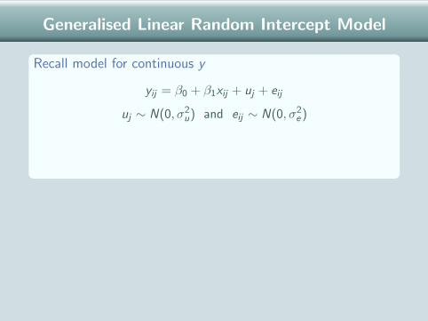
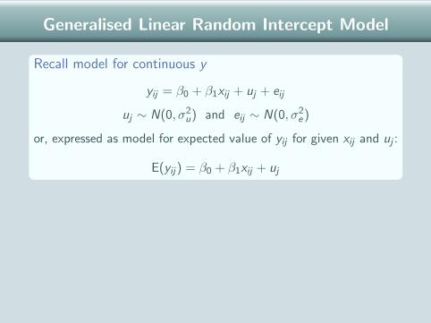
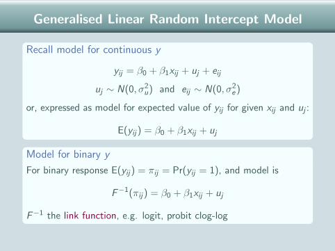
Recall model for continuous y
yij = β0 + β1xij + uj + eij
uj ∼ N(0, σ2u) and eij ∼ N(0, σ2
e )
or, expressed as model for expected value of yij for given xij and uj :
E(yij) = β0 + β1xij + uj
Model for binary y
For binary response E(yij) = πij = Pr(yij = 1), and model is
F−1(πij) = β0 + β1xij + uj
F−1 the link function, e.g. logit, probit clog-log
Generalised Linear Random Intercept Model
Recall model for continuous y
yij = β0 + β1xij + uj + eij
uj ∼ N(0, σ2u) and eij ∼ N(0, σ2
e )
or, expressed as model for expected value of yij for given xij and uj :
E(yij) = β0 + β1xij + uj
Model for binary y
For binary response E(yij) = πij = Pr(yij = 1), and model is
F−1(πij) = β0 + β1xij + uj
F−1 the link function, e.g. logit, probit clog-log

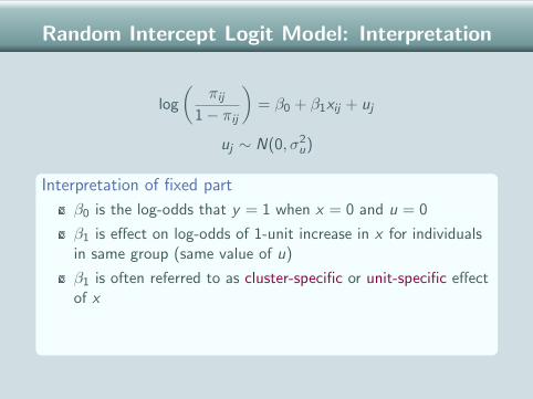
Random Intercept Logit Model: Interpretation
log
(πij
1− πij
)= β0 + β1xij + uj
uj ∼ N(0, σ2u)
Interpretation of fixed part
β0 is the log-odds that y = 1 when x = 0 and u = 0
β1 is effect on log-odds of 1-unit increase in x for individualsin same group (same value of u)
β1 is often referred to as cluster-specific or unit-specific effectof x
exp(β1) is an odds ratio, comparing odds for individualsspaced 1-unit apart on x but in the same group
Random Intercept Logit Model: Interpretation
log
(πij
1− πij
)= β0 + β1xij + uj
uj ∼ N(0, σ2u)
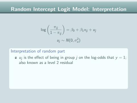
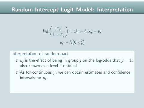
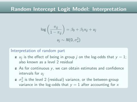
Interpretation of random part
uj is the effect of being in group j on the log-odds that y = 1;also known as a level 2 residual
As for continuous y , we can obtain estimates and confidenceintervals for uj
σ2u is the level 2 (residual) variance, or the between-group
variance in the log-odds that y = 1 after accounting for x
Random Intercept Logit Model: Interpretation
log
(πij
1− πij
)= β0 + β1xij + uj
uj ∼ N(0, σ2u)
Interpretation of random part
uj is the effect of being in group j on the log-odds that y = 1;also known as a level 2 residual
As for continuous y , we can obtain estimates and confidenceintervals for uj
σ2u is the level 2 (residual) variance, or the between-group
variance in the log-odds that y = 1 after accounting for x

Response Probabilities from Logit Model
Response probability for individual i in group j calculated as
πij =exp(β0 + β1xij + uj)
1 + exp(β0 + β1xij + uj)
Substitute estimates of β0, β1 and uj to get predicted probability:
πij =exp(β0 + β1xij + uj)
1 + exp(β0 + β1xij + uj)
We can also make predictions for ‘ideal’ or ‘typical’ individuals withparticular values for x , but we need to decide what to substitutefor uj (discussed later).

Example: US Voting Intentions
Individuals (at level 1) within states (at level 2).
Results from null logit model (no x)
Parameter Estimate se
β0 (intercept) -0.107 0.049σ2
u (between-state variance) 0.091 0.023
Questions about σ2u
1. Is σ2u significantly different from zero?
2. Does σ2u = 0.09 represent a large state effect?
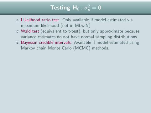
Testing H0 : σ2u = 0
Likelihood ratio test. Only available if model estimated viamaximum likelihood (not in MLwiN)
Wald test (equivalent to t-test), but only approximate becausevariance estimates do not have normal sampling distributionsBayesian credible intervals. Available if model estimated usingMarkov chain Monte Carlo (MCMC) methods.
Example
Wald statistic =
(σ2
u
se
)2
=
(0.091
0.023
)2
= 15.65
Compare with χ21 → reject H0 and conclude there are state
differences.
Take p-value/2 because alternative hypothesis is one-sided(HA : σ2
u > 0)

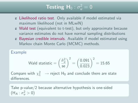
Testing H0 : σ2u = 0
Likelihood ratio test. Only available if model estimated viamaximum likelihood (not in MLwiN)Wald test (equivalent to t-test), but only approximate becausevariance estimates do not have normal sampling distributions
Bayesian credible intervals. Available if model estimated usingMarkov chain Monte Carlo (MCMC) methods.
Example
Wald statistic =
(σ2
u
se
)2
=
(0.091
0.023
)2
= 15.65
Compare with χ21 → reject H0 and conclude there are state
differences.
Take p-value/2 because alternative hypothesis is one-sided(HA : σ2
u > 0)
Testing H0 : σ2u = 0
Likelihood ratio test. Only available if model estimated viamaximum likelihood (not in MLwiN)Wald test (equivalent to t-test), but only approximate becausevariance estimates do not have normal sampling distributionsBayesian credible intervals. Available if model estimated usingMarkov chain Monte Carlo (MCMC) methods.
Example
Wald statistic =
(σ2
u
se
)2
=
(0.091
0.023
)2
= 15.65
Compare with χ21 → reject H0 and conclude there are state
differences.
Take p-value/2 because alternative hypothesis is one-sided(HA : σ2
u > 0)

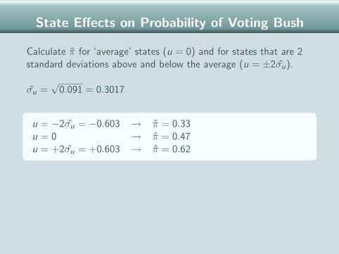
State Effects on Probability of Voting Bush
Calculate π for ‘average’ states (u = 0) and for states that are 2standard deviations above and below the average (u = ±2σu).
σu =√
0.091 = 0.3017
u = −2σu = −0.603 → π = 0.33u = 0 → π = 0.47u = +2σu = +0.603 → π = 0.62
Under a normal distribution assumption, expect 95% of states tohave π within (0.33, 0.62).
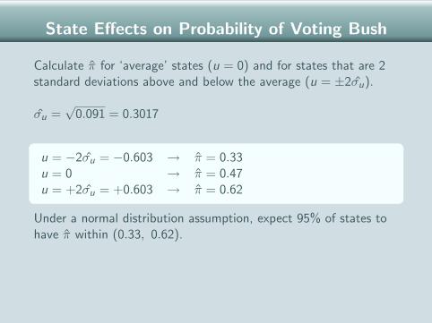

uj with 95% Confidence Intervals for uj

Adding Income as a Predictor
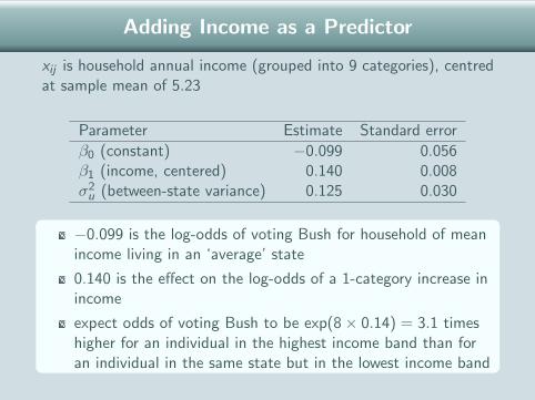
xij is household annual income (grouped into 9 categories), centredat sample mean of 5.23
Parameter Estimate Standard error
β0 (constant) −0.099 0.056β1 (income, centered) 0.140 0.008σ2
u (between-state variance) 0.125 0.030
−0.099 is the log-odds of voting Bush for household of meanincome living in an ‘average’ state
0.140 is the effect on the log-odds of a 1-category increase inincome
expect odds of voting Bush to be exp(8× 0.14) = 3.1 timeshigher for an individual in the highest income band than foran individual in the same state but in the lowest income band

Adding Income as a Predictor
xij is household annual income (grouped into 9 categories), centredat sample mean of 5.23
Parameter Estimate Standard error
β0 (constant) −0.099 0.056β1 (income, centered) 0.140 0.008σ2
u (between-state variance) 0.125 0.030
−0.099 is the log-odds of voting Bush for household of meanincome living in an ‘average’ state
0.140 is the effect on the log-odds of a 1-category increase inincome
expect odds of voting Bush to be exp(8× 0.14) = 3.1 timeshigher for an individual in the highest income band than foran individual in the same state but in the lowest income band
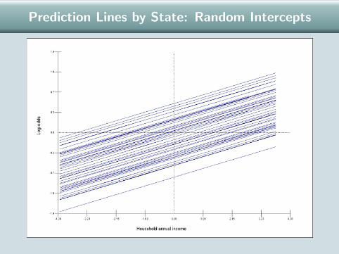
Prediction Lines by State: Random Intercepts

Latent Variable Representation
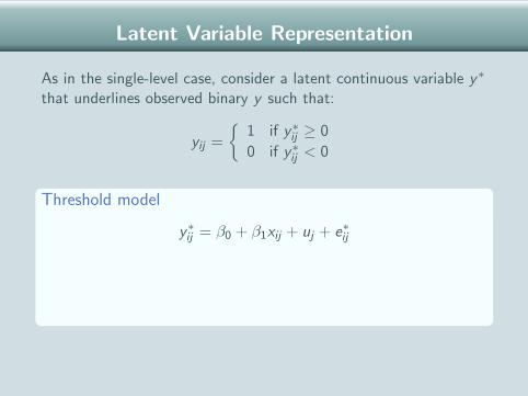
As in the single-level case, consider a latent continuous variable y∗
that underlines observed binary y such that:
yij =
{1 if y∗ij ≥ 0
0 if y∗ij < 0
Threshold model
y∗ij = β0 + β1xij + uj + e∗ij
As in a single-level model:
e∗ij ∼ N(0, 1) → probit model
e∗ij ∼ standard logistic (with variance ' 3.29) → logit model
So the level 1 residual variance, var(e∗ij), is fixed.
Latent Variable Representation
As in the single-level case, consider a latent continuous variable y∗
that underlines observed binary y such that:
yij =
{1 if y∗ij ≥ 0
0 if y∗ij < 0
Threshold model
y∗ij = β0 + β1xij + uj + e∗ij
As in a single-level model:
e∗ij ∼ N(0, 1) → probit model
e∗ij ∼ standard logistic (with variance ' 3.29) → logit model
So the level 1 residual variance, var(e∗ij), is fixed.

Impact of Adding uj on Coefficients
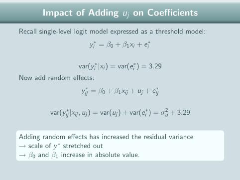
Recall single-level logit model expressed as a threshold model:
y∗i = β0 + β1xi + e∗i
var(y∗i |xi ) = var(e∗i ) = 3.29
Now add random effects:
y∗ij = β0 + β1xij + uj + e∗ij
var(y∗ij |xij , uj) = var(uj) + var(e∗i ) = σ2u + 3.29
Adding random effects has increased the residual variance→ scale of y∗ stretched out→ β0 and β1 increase in absolute value.

Impact of Adding uj on Coefficients
Recall single-level logit model expressed as a threshold model:
y∗i = β0 + β1xi + e∗i
var(y∗i |xi ) = var(e∗i ) = 3.29
Now add random effects:
y∗ij = β0 + β1xij + uj + e∗ij
var(y∗ij |xij , uj) = var(uj) + var(e∗i ) = σ2u + 3.29
Adding random effects has increased the residual variance→ scale of y∗ stretched out→ β0 and β1 increase in absolute value.

Single-level vs Random Intercept Coefficients
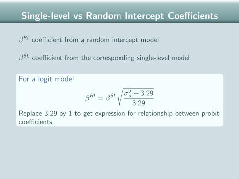
βRI coefficient from a random intercept model
βSL coefficient from the corresponding single-level model
For a logit model
βRI = βSL
√σ2
u + 3.29
3.29
Replace 3.29 by 1 to get expression for relationship between probitcoefficients.
NOTE: Adding random effects to a continuous response modeldoes not ‘scale up’ coefficients because the level 1 variance is notfixed and so: var(ei ) ' var(uj) + var(eij)
Single-level vs Random Intercept Coefficients
βRI coefficient from a random intercept model
βSL coefficient from the corresponding single-level model
For a logit model
βRI = βSL
√σ2
u + 3.29
3.29
Replace 3.29 by 1 to get expression for relationship between probitcoefficients.
NOTE: Adding random effects to a continuous response modeldoes not ‘scale up’ coefficients because the level 1 variance is notfixed and so: var(ei ) ' var(uj) + var(eij)

Single-level vs Random Intercept Coefficients
Simulated data where distribution of x1 and x2 same in each level2 unit.
σ2u = 1.018 so expected RI:SL ratio is
√1.018+3.29
3.29 = 1.14
Variable βSL βRI βRI/βSL
Constant 0.221 0.257 1.163x1 0.430 0.519 1.207x2 0.498 0.613 1.231
In practice, RI:SL ratio for a given x may be quite different fromthat expected if distribution of x differs across level 2 units.

Impact of Adding level 1 x
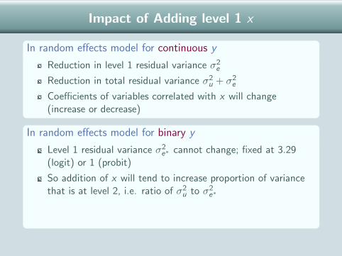
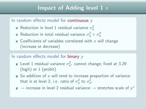
In random effects model for continuous y
Reduction in level 1 residual variance σ2e
Reduction in total residual variance σ2u + σ2
e
Coefficients of variables correlated with x will change(increase or decrease)
In random effects model for binary y
Level 1 residual variance σ2e∗ cannot change; fixed at 3.29
(logit) or 1 (probit)
So addition of x will tend to increase proportion of variancethat is at level 2, i.e. ratio of σ2
u to σ2e∗
→ increase in level 2 residual variance → stretches scale of y∗
→ increase in absolute value of coefficients of other variables

Impact of Adding level 1 x
In random effects model for continuous y
Reduction in level 1 residual variance σ2e
Reduction in total residual variance σ2u + σ2
e
Coefficients of variables correlated with x will change(increase or decrease)
In random effects model for binary y
Level 1 residual variance σ2e∗ cannot change; fixed at 3.29
(logit) or 1 (probit)
So addition of x will tend to increase proportion of variancethat is at level 2, i.e. ratio of σ2
u to σ2e∗
→ increase in level 2 residual variance → stretches scale of y∗
→ increase in absolute value of coefficients of other variables

Variance Partition Coefficient for Binary y
Usual formula is:
VPC =level 2 residual variance
level 1 residual variance + level 2 residual variance
From threshold model for latent y ∗, we obtain
VPC =σ2
u
σ2e∗ + σ2
u
where σ2e∗ = 1 for probit model and 3.29 for logit model
In voting intentions example, σ2u=0.125, so VPC=0.037. Adjusting
for income, 4% of the remaining variance in the propensity to voteBush is attributable to between-state variation.
Marginal Model for Clustered y
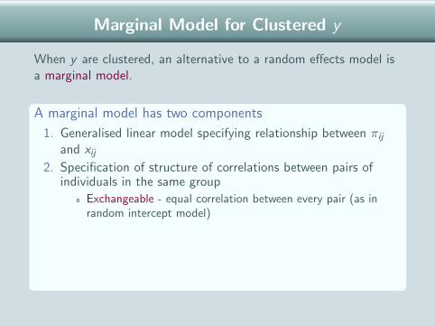
When y are clustered, an alternative to a random effects model isa marginal model.
A marginal model has two components
1. Generalised linear model specifying relationship between πij
and xij
2. Specification of structure of correlations between pairs ofindividuals in the same group
Exchangeable - equal correlation between every pair (as inrandom intercept model)Autocorrelation - used for longitudinal data where correlation afunction of time between measuresUnstructured - all pairwise correlations estimated
Estimated using Generalised Estimating Equations (GEE)

Marginal Model for Clustered y
When y are clustered, an alternative to a random effects model isa marginal model.
A marginal model has two components
1. Generalised linear model specifying relationship between πij
and xij
2. Specification of structure of correlations between pairs ofindividuals in the same group
Exchangeable - equal correlation between every pair (as inrandom intercept model)Autocorrelation - used for longitudinal data where correlation afunction of time between measuresUnstructured - all pairwise correlations estimated
Estimated using Generalised Estimating Equations (GEE)
Marginal Model for Clustered y
When y are clustered, an alternative to a random effects model isa marginal model.
A marginal model has two components
1. Generalised linear model specifying relationship between πij
and xij
2. Specification of structure of correlations between pairs ofindividuals in the same group
Exchangeable - equal correlation between every pair (as inrandom intercept model)
Autocorrelation - used for longitudinal data where correlation afunction of time between measuresUnstructured - all pairwise correlations estimated
Estimated using Generalised Estimating Equations (GEE)

Marginal Model for Clustered y
When y are clustered, an alternative to a random effects model isa marginal model.
A marginal model has two components
1. Generalised linear model specifying relationship between πij
and xij
2. Specification of structure of correlations between pairs ofindividuals in the same group
Exchangeable - equal correlation between every pair (as inrandom intercept model)Autocorrelation - used for longitudinal data where correlation afunction of time between measures
Unstructured - all pairwise correlations estimated
Estimated using Generalised Estimating Equations (GEE)

Marginal Model for Clustered y
When y are clustered, an alternative to a random effects model isa marginal model.
A marginal model has two components
1. Generalised linear model specifying relationship between πij
and xij
2. Specification of structure of correlations between pairs ofindividuals in the same group
Exchangeable - equal correlation between every pair (as inrandom intercept model)Autocorrelation - used for longitudinal data where correlation afunction of time between measuresUnstructured - all pairwise correlations estimated
Estimated using Generalised Estimating Equations (GEE)
Marginal vs Random Effects Approaches
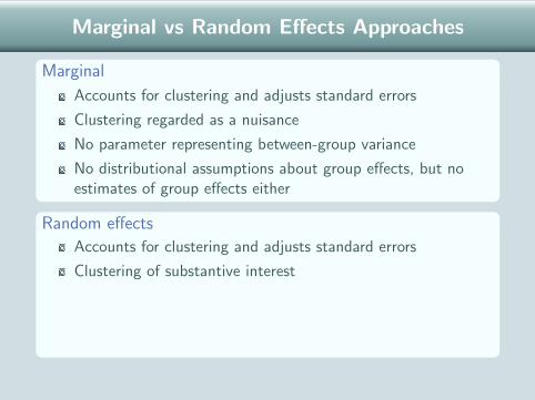
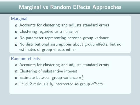
Marginal
Accounts for clustering and adjusts standard errors
Clustering regarded as a nuisance
No parameter representing between-group variance
No distributional assumptions about group effects, but noestimates of group effects either
Random effects
Accounts for clustering and adjusts standard errors
Clustering of substantive interest
Estimate between-group variance σ2u
Level 2 residuals uj interpreted as group effects
Can allow between-group variance to depend on x

Marginal vs Random Effects Approaches
Marginal
Accounts for clustering and adjusts standard errors
Clustering regarded as a nuisance
No parameter representing between-group variance
No distributional assumptions about group effects, but noestimates of group effects either
Random effects
Accounts for clustering and adjusts standard errors
Clustering of substantive interest
Estimate between-group variance σ2u
Level 2 residuals uj interpreted as group effects
Can allow between-group variance to depend on x

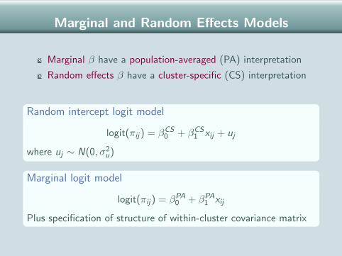
Marginal and Random Effects Models
Marginal β have a population-averaged (PA) interpretation
Random effects β have a cluster-specific (CS) interpretation
Random intercept logit model
logit(πij) = βCS0 + βCS
1 xij + uj
where uj ∼ N(0, σ2u)
Marginal logit model
logit(πij) = βPA0 + βPA
1 xij
Plus specification of structure of within-cluster covariance matrix

Interpretation of CS and PA Effects
Cluster-specific
βCS1 is the effect of a 1-unit change in x on the log-odds that
y = 1 for a given cluster, i.e. holding constant (orconditioning on) cluster-specific unobservables
βCS1 contrasts two individuals in the same cluster with
x-values 1 unit apart
Population-averaged
βPA1 is the effect of a 1-unit change in x on the log-odds that
y = 1 in the study population, i.e. averaging overcluster-specific unobservables

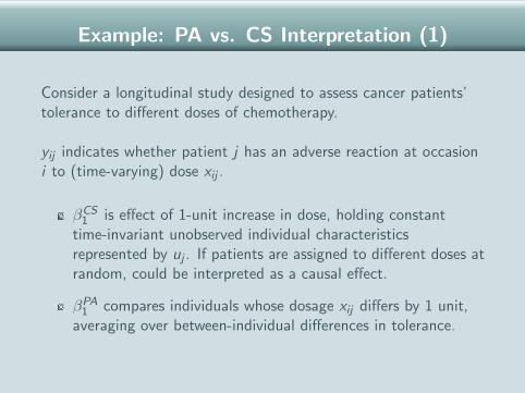
Example: PA vs. CS Interpretation (1)
Consider a longitudinal study designed to assess cancer patients’tolerance to different doses of chemotherapy.
yij indicates whether patient j has an adverse reaction at occasioni to (time-varying) dose xij .
βCS1 is effect of 1-unit increase in dose, holding constant
time-invariant unobserved individual characteristicsrepresented by uj . If patients are assigned to different doses atrandom, could be interpreted as a causal effect.
βPA1 compares individuals whose dosage xij differs by 1 unit,
averaging over between-individual differences in tolerance.
Example: PA vs. CS Interpretation (2)
Suppose we add a level 2 variable, gender (x2j), with coefficient β2.
Because x2j is fixed over time, we cannot interpret βCS2 as a
within-person effect. Instead βCS2 compares men and women
with the same value of xij and uj , i.e. the same dose and thesame combination of unobserved time-invariantcharacteristics.
βPA2 compares men and women receiving the same dose xij ,
averaging over individual unobservables.
For a level 2 variable, βPA2 may be of more interest.

Comparison of PA and CS Coefficients
In general |βCS | > |βPA|
The relationship between the CS and PA logit coefficients fora variable x is approximately:
βCS =
√σ2
u + 3.29
3.29βPA
When there is no clustering, σ2u = 0 and βCS = βPA.
Coefficients move further apart as σ2u increases
Note that marginal models can also be specified for continuousy , but in that case CS and PA coefficients are equal

Predictions from a Multilevel Model
Response probability for individual i in group j calculated as
πij =exp(β0 + β1xij + uj)
1 + exp(β0 + β1xij + uj)
where we substitute estimates of β0, β1 and uj to get predictedprobabilities.
Rather than calculating probabilities for each individual, however,we often want predictions for specific values of x . But what do wesubstitute for uj?

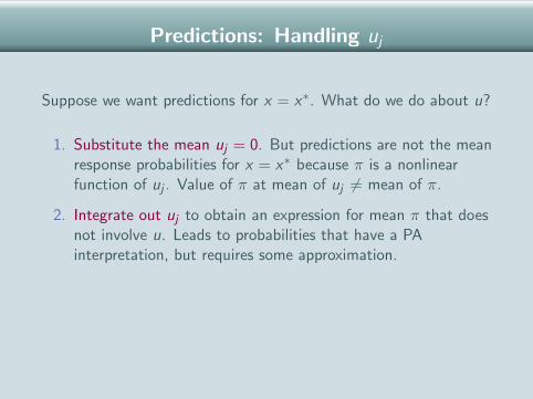
Predictions: Handling uj
Suppose we want predictions for x = x∗. What do we do about u?
1. Substitute the mean uj = 0. But predictions are not the meanresponse probabilities for x = x∗ because π is a nonlinearfunction of uj . Value of π at mean of uj 6= mean of π.
2. Integrate out uj to obtain an expression for mean π that doesnot involve u. Leads to probabilities that have a PAinterpretation, but requires some approximation.
3. Average over simulated values of uj . Also gives PAprobabilities, but easier to implement. Now available inMLwiN.

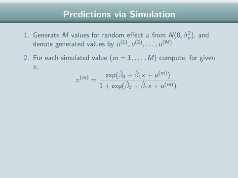
Predictions via Simulation
1. Generate M values for random effect u from N(0, σ2u), and
denote generated values by u(1), u(2), . . . , u(M)
2. For each simulated value (m = 1, . . . ,M) compute, for givenx ,
π(m) =exp(β0 + β1x + u(m))
1 + exp(β0 + β1x + u(m))
3. Calculate the mean of π(m):
π =1
M
M∑m=1
π(m)
4. Repeat 1-3 for different value of x
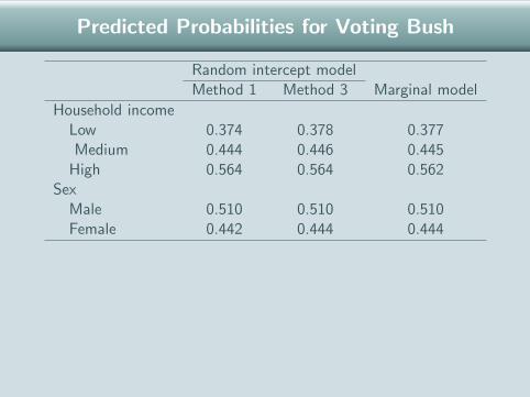
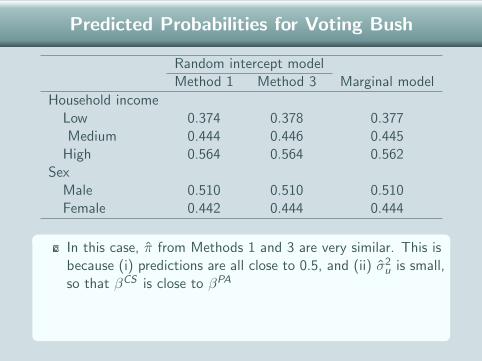
Predicted Probabilities for Voting Bush
Random intercept modelMethod 1 Method 3 Marginal model
Household incomeLow 0.374 0.378 0.377Medium 0.444 0.446 0.445
High 0.564 0.564 0.562Sex
Male 0.510 0.510 0.510Female 0.442 0.444 0.444
In this case, π from Methods 1 and 3 are very similar. This isbecause (i) predictions are all close to 0.5, and (ii) σ2
u is small,so that βCS is close to βPA
In longitudinal applications, where σ2u can be large, there will
be bigger differences between Methods 1 and 3

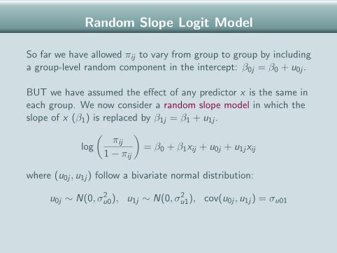
Random Slope Logit Model
So far we have allowed πij to vary from group to group by includinga group-level random component in the intercept: β0j = β0 + u0j .
BUT we have assumed the effect of any predictor x is the same ineach group. We now consider a random slope model in which theslope of x (β1) is replaced by β1j = β1 + u1j .
log
(πij
1− πij
)= β0 + β1xij + u0j + u1jxij
where (u0j , u1j) follow a bivariate normal distribution:
u0j ∼ N(0, σ2u0), u1j ∼ N(0, σ2
u1), cov(u0j , u1j) = σu01
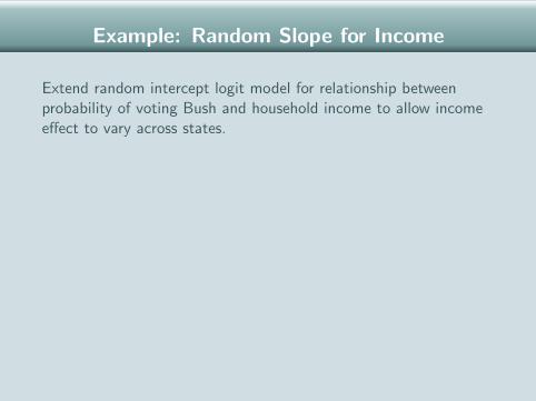
Example: Random Slope for Income
Extend random intercept logit model for relationship betweenprobability of voting Bush and household income to allow incomeeffect to vary across states.
Random int. Random slopeParameter Est. se Est. se
β0 (constant) −0.099 0.056 −0.087 0.057β1 (Income, centred) 0.140 0.008 0.145 0.013
State-level random partσ2
u0 (intercept variance) 0.125 0.031 0.132 0.032σ2
u1 (slope variance) - - 0.003 0.001σu01 (intercept-slope covariance) - - 0.018 0.006
Testing for a Random Slope
Allowing x to have a random slope introduces 2 new parameters:σ2
u1 and σu01.
Test H0 : σ2u1 = σu01 = 0 using a likelihood ratio test or
(approximate) Wald test on 2 d.f.
For the income example, Wald = 9.72. Comparing with χ22 gives a
two-sided p-value of 0.0008
=⇒ income effect does vary across states.

Prediction Lines by State: Random Slopes

Intercept vs. Income Slope Residuals
Bottom left: Washington DC
Top right: Montana and Utah

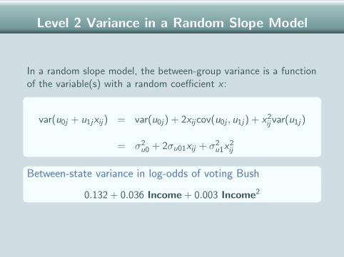
Level 2 Variance in a Random Slope Model
In a random slope model, the between-group variance is a functionof the variable(s) with a random coefficient x :
var(u0j + u1jxij) = var(u0j) + 2xijcov(u0j , u1j) + x2ij var(u1j)
= σ2u0 + 2σu01xij + σ2
u1x2ij
Between-state variance in log-odds of voting Bush
0.132 + 0.036 Income + 0.003 Income2

Between-State Variance by Income

Adding a Level 2 x : Contextual Effects
A major advantage of the multilevel approach is the ability toexplore effects of group-level (level 2) predictors, while accountingfor the effects of unobserved group characteristics.
A random intercept logit model with a level 1 variable x1ij and alevel 2 variable x2j is:
log
(πij
1− πij
)= β0 + β1x1ij + β2x2j + uj
β2 is the contextual effect of x2j .
Especially important to use a multilevel model if interested incontextual effects as se(β2) may be severely estimated if asingle-level model is used.

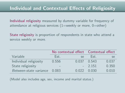
Individual and Contextual Effects of Religiosity
Individual religiosity measured by dummy variable for frequency ofattendance at religious services (1=weekly or more, 0=other)
State religiosity is proportion of respondents in state who attend aservice weekly or more.
No contextual effect Contextual effectVariable Est. se Est. se
Individual religiosity 0.556 0.037 0.543 0.037State religiosity - - 2.151 0.350Between-state variance 0.083 0.022 0.030 0.010
(Model also includes age, sex, income and marital status.)

Cross-Level Interactions
Suppose we believe that the effect of an individual characteristicon πij depends on the value of a group characteristic.
We can extend the contextual effects model to allow the effect ofx1ij to depend on x2j by including a cross-level interaction:
log
(πij
1− πij
)= β0 + β1x1ij + β2x2j + β3x1ijx2j + uj
The null hypothesis for a test of a cross-level interaction isH0 : β3 = 0.

Example of Cross-Level Interaction
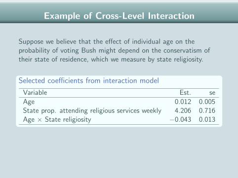
Suppose we believe that the effect of individual age on theprobability of voting Bush might depend on the conservatism oftheir state of residence, which we measure by state religiosity.
Selected coefficients from interaction model
Variable Est. se
Age 0.012 0.005State prop. attending religious services weekly 4.206 0.716Age × State religiosity −0.043 0.013
Z-ratio for interaction coefficient is 0.043/0.013 = 3.31 which ishighly significant =⇒ effect of age depends on state religiosity.
Example of Cross-Level Interaction
Suppose we believe that the effect of individual age on theprobability of voting Bush might depend on the conservatism oftheir state of residence, which we measure by state religiosity.
Selected coefficients from interaction model
Variable Est. se
Age 0.012 0.005State prop. attending religious services weekly 4.206 0.716Age × State religiosity −0.043 0.013
Z-ratio for interaction coefficient is 0.043/0.013 = 3.31 which ishighly significant =⇒ effect of age depends on state religiosity.

Effect of Age by State Religiosity
Age effects on log-odds of voting Bush
Proportion attending Age Effectservices weekly
0.16 0.012 − (0.043 × 0.16) = 0.0050.30 0.012 − (0.043 × 0.30) = −0.00090.64 0.012 − (0.043 × 0.64) = −0.016
So age effect is weakly positive for the least religious states, andbecomes less strongly positive and then more strongly negative asstate-level religiosity increases.
=⇒ Difference between young and old respondents in votingintentions is greatest in most religious states.

A Brief Overview of Estimation Procedures
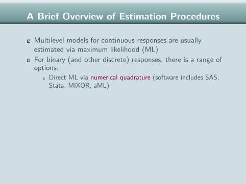
Multilevel models for continuous responses are usuallyestimated via maximum likelihood (ML)
For binary (and other discrete) responses, there is a range ofoptions:
Direct ML via numerical quadrature (software includes SAS,Stata, MIXOR, aML)Quasi-likelihood (MLwiN, HLM)Markov chain Monte Carlo (MCMC) methods (WinBUGS,MLwiN)
In some situations, different procedures can lead to quitedifferent results

A Brief Overview of Estimation Procedures
Multilevel models for continuous responses are usuallyestimated via maximum likelihood (ML)
For binary (and other discrete) responses, there is a range ofoptions:
Direct ML via numerical quadrature (software includes SAS,Stata, MIXOR, aML)Quasi-likelihood (MLwiN, HLM)Markov chain Monte Carlo (MCMC) methods (WinBUGS,MLwiN)
In some situations, different procedures can lead to quitedifferent results
A Brief Overview of Estimation Procedures
Multilevel models for continuous responses are usuallyestimated via maximum likelihood (ML)
For binary (and other discrete) responses, there is a range ofoptions:
Direct ML via numerical quadrature (software includes SAS,Stata, MIXOR, aML)
Quasi-likelihood (MLwiN, HLM)Markov chain Monte Carlo (MCMC) methods (WinBUGS,MLwiN)
In some situations, different procedures can lead to quitedifferent results

A Brief Overview of Estimation Procedures
Multilevel models for continuous responses are usuallyestimated via maximum likelihood (ML)
For binary (and other discrete) responses, there is a range ofoptions:
Direct ML via numerical quadrature (software includes SAS,Stata, MIXOR, aML)Quasi-likelihood (MLwiN, HLM)
Markov chain Monte Carlo (MCMC) methods (WinBUGS,MLwiN)
In some situations, different procedures can lead to quitedifferent results

A Brief Overview of Estimation Procedures
Multilevel models for continuous responses are usuallyestimated via maximum likelihood (ML)
For binary (and other discrete) responses, there is a range ofoptions:
Direct ML via numerical quadrature (software includes SAS,Stata, MIXOR, aML)Quasi-likelihood (MLwiN, HLM)Markov chain Monte Carlo (MCMC) methods (WinBUGS,MLwiN)
In some situations, different procedures can lead to quitedifferent results

Comparison of Quasi-Likelihood Methods
Rodrıguez and Goldman (2001, J. Roy. Stat. Soc.) simulated a3-level data structure with 2449 births (level 1) from 1558 mothers(level 2) in 161 communities (level 3), and one predictor at eachlevel.
Results from 100 simulations
Parameter True value MQL1 MQL2 PQL2
Child-level x 1 0.74 0.85 0.96Family-level x 1 0.74 0.86 0.96Community-level x 1 0.77 0.91 0.96Random effect st. dev.Family 1 0.10 0.28 0.73Community 1 0.73 0.76 0.93

Comparison of Estimation Procedures
Rodrıguez and Goldman (2001) also analysed real data on childimmunisation in Guatemala.
Random effect standard deviations
PQL2 PQL1-B ML MCMC
Family 1.75 2.69 2.32 2.60Community 0.84 1.06 1.02 1.13
PQL-B is PQL with a bias correction; ML is maximum likelihood;MCMC is Markov chain Monte Carlo (Gibbs sampling)
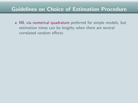
Guidelines on Choice of Estimation Procedure
ML via numerical quadrature preferred for simple models, butestimation times can be lengthy when there are severalcorrelated random effects
Quasi-likelihood methods quick and useful for modelscreening, but biased (especially for small cluster sizes)
MCMC methods are flexible and becoming increasinglycomputationally feasible; the recommended method in MLwiN