multilevel models

Multilevel Models

David M. Rocke

May 27, 2021

David M. Rocke Multilevel Models May 27, 2021 1 / 33

Multilevel Models

A good reference on this topic is Data Analysisusing Regression and Multilevel/Hierarchical Modelsby Andrew Gelman and Jennifer Hill, 2007,Cambridge University Press.

The software orientation is both with using lmer inR or using bugs called from R.

Bugs is a set of programs for Bayesian analysis ofstatistical problems. It can sometimes solveproblems that are not easily handled in frequentiststatistics, but it also can be very slow, and does notalways give an answer.

We will concentrate on analysis using lmer.David M. Rocke Multilevel Models May 27, 2021 2 / 33

Multilevel Models

Multilevel models are those in which individualsobservations exist in groups.

The individuals have potential predictors, but therelationship of the predictor to the prediction can bedifferent in different groups.

The intercepts may be different, so that allindividuals in one group may have on the averagehigher levels of the response.

The slopes (coefficients) may be different betweengroups as well, as in a group-by-predictorinteraction.


Radon Data Set

This is a processed subset of the srrs2.dat data set ofindividual home radon levels in the US. These values arefor Minnesota only, and we are interested in householdand county level analysis.

Variable Definitionradon Radon level in individual homelog.radon Log-radon or log(0.1) if radon=0floor 0 = basement, 1 = first floorcounty.name Name of each of 85 countiescounty county number, 1–85


Data Input

## Read & clean the data

# get radon data

# Data are at http://www.stat.columbia.edu/~gelman/arm/examples/radon

#library ("arm")

srrs2 <- read.table ("srrs2.dat", header=T, sep=",")

mn <- srrs2$state=="MN"

radon <- srrs2$activity[mn]

log.radon <- log (ifelse (radon==0, .1, radon))

# The six lowest values of radon are 0, 0 , 0, 0.1, 0.2, 0.2

# replace 0 value by lowest non-zero value or half lowest

floor <- srrs2$floor[mn] # 0 for basement, 1 for first floor

n <- length(radon)


Data Input

# get county index variable

county.name <- as.vector(srrs2$county[mn])

# as.vector converts factor into character

# needed since factor levels would include county names for all US counties

uniq <- unique(county.name)

# county name occurs as many times as there are houses in county

# data are already sorted by county, else we could use sort(unique())

J <- length(uniq)

county <- rep (NA, J)

for (i in 1:J){

county[county.name==uniq[i]] <- i

}

radondf <- data.frame(radon,log.radon,floor,county.name,county)


> summary(radondf)

radon log.radon floor

Min. : 0.000 Min. :-2.3026 Min. :0.0000

1st Qu.: 1.900 1st Qu.: 0.6419 1st Qu.:0.0000

Median : 3.600 Median : 1.2809 Median :0.0000

Mean : 4.768 Mean : 1.2246 Mean :0.1665

3rd Qu.: 6.000 3rd Qu.: 1.7918 3rd Qu.:0.0000

Max. :48.200 Max. : 3.8754 Max. :1.0000

county.name county

ST LOUIS :116 Min. : 1.00

HENNEPIN :105 1st Qu.:21.00

DAKOTA : 63 Median :44.00

ANOKA : 52 Mean :43.52

WASHINGTON : 46 3rd Qu.:70.00

RAMSEY : 32 Max. :85.00

(Other) :505


Types of Analysis

If we want to know the distribution of radon levels,we can pool the data from all 85 counties.

Or we can analyze each county separately(unpooled).

We can also have a varying intercept for county, butuse a pooled error variance.

Or we can use a two-level model for houses andcounties, which is in effect partially pooled.

In each case, we can add one or more covariates.


Pooled Analysis

pool1 <- function(){

# pooled analysis

print(mean(log.radon))

print(sd(log.radon))

pdf("pooled.hist.pdf")

hist(log.radon)

dev.off()

}

> pool1()

[1] 1.224623 #mean log radon level across all 919 households

[1] 0.8533272 #standard deviation of log radon level

This does not allow any analysis of which counties have the highest radon levels.


Histogram of log.radon

log.radon

Fre

quen

cy

−2 −1 0 1 2 3 4

050

100

150

200


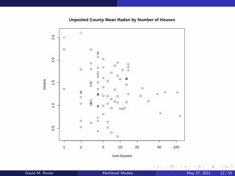
Unpooled Analysis

nopool1 <- function(){

num.houses <- as.vector(table(county))

# table counts the number of data points for each value of county

means <- tapply(log.radon,county,mean)

# tapply applies a function (mean) of the set of the first argument (log.radon)

# for each value of the second entry (county)

sds <- tapply(log.radon,county,sd)

pdf("meanVN.pdf")

plot(num.houses,means,log="x")

title("Unpooled County Mean Radon by Number of Houses")

dev.off()

}

> nopool1()


1 2 5 10 20 50 100

0.5

1.0

1.5

2.0

2.5

num.houses

mea

ns

Unpooled County Mean Radon by Number of Houses


Unpooled Analysis

nopool1 <- function(){


means <- tapply(log.radon,county,mean)

sds <- tapply(log.radon,county,sd)

pdf("meanVN.pdf")

plot(num.houses,means,log="x",col=ifelse(means > 2.3,"red","black"))

title("Unpooled County Mean Radon by Number of Houses")

dev.off()

print(which(means > 2.3))

print(county.name[county==50])

print(county.name[county==36])

}

> nopool1()

36 50

36 50

[1] "MURRAY "

[1] "LAC QUI PARLE " "LAC QUI PARLE "

Two highest radon means have one or two houses per county.

This is probably chance variation.


1 2 5 10 20 50 100

0.5

1.0

1.5

2.0

2.5

num.houses

mea

ns



Partial Pooling

We allow each county to have its own intercept (averagelevel) which we treat as random.

partialpool1 <- function(){

require(lme4)

radon.lmer <- lmer(log.radon ~ 1 + (1|county))

preds <- predict(radon.lmer)


ctypreds <- tapply(preds,county,mean)

pdf("ctypredsVN.pdf")

plot(num.houses,ctypreds,log="x")

title("Pooled County Radon Mean Prediction by Number of Houses")

dev.off()

}


1 2 5 10 20 50 100

0.8

1.0

1.2

1.4

1.6

num.houses

ctyp

reds

Pooled County Radon Mean Prediction by Number of Houses


1 2 5 10 20 50 100

0.5

1.0

1.5

2.0

2.5

num.houses

mea

ns



Sample Size by County

Three counties have one house, eight counties havetwo houses, and eleven counties have 3 houses. Twoof the 87 have no houses in the sample.

St. Louis County has 116 houses. It is largest by afactor of two and sixth in population (Duluth).

The next three largest counties have 7, 11, and 7houses. They are 61st, 22nd, and 21st inpopulation.

Hennepin County (Minneapolis) has 105 houses.

The next three most populous counties have 32, 63,and 52 houses, but they are 87th, 58th, and 81st inland area out of 87 counties..


Comparison of Pooling, No Pooling,Partial Pooling

The mean log radon level across all counties is 1.225.The table shows the two highest and three lowestcounties in mean radon level.

County Pooled Unpooled Partially PooledLac Qui Parle 1.225 2.599 1.610Murray 1.225 2.493 1.467Waseca 1.225 0.435 0.983Koochiching 1.225 0.407 0.848Lake 1.225 0.322 0.743


poolcomp <- function(){

require(lme4)

radon.lmer <- lmer(log.radon ~ 1 + (1|county))

preds <- predict(radon.lmer)


ctypreds <- tapply(preds,county,mean)

poolpred <- mean(log.radon)

unpoolpred <- tapply(log.radon,county,mean)

predvec <- c(unpoolpred,ctypreds)

n <- length(ctypreds)

poolmeth <- rep(0:1,each=n)

pdf("poolcomp.pdf")

plot(poolmeth,predvec,xlab="Pooling Method",type="p",xaxt="n",xlim=c(-.1,1.1))

axis(1,at=c(0,1),labels=c("Unpooled","Partially Pooled"))

abline(h=poolpred,lwd=2,col="blue")

arrows(0,unpoolpred,1,ctypreds)

title("Estimated Mean Log Radon Level by Pooling Method")

dev.off()

}


0.5

1.0

1.5

2.0

2.5

Pooling Method

pred

vec

Unpooled Partially Pooled

Estimated Mean Log Radon Level by Pooling Method


Partially Pooled via lmer

The predicted value for each observation in a countyis a linear combination of the individual countymean (unpooled) and the pooled grand mean.

Each county mean is “shrunk” towards the center.

The county individual mean has a weight of thesamples size in the county, which is inverselyproportional to the variance of the county mean.

Counties with a small number of data points aremore shrunk than counties with a large number ofdata points.


Using Individual-Level Covariates

The variable floor indicates whether the radonreading was taken in the basement, where it likelywould be higher, or on the first floor.

We could add this as a covariate and also if wechose we could make the coefficient of this covariatedepend on the county.

Individual county analysis might not be able toestimate the coefficient of floor because 25 of the85 counties have no houses with data from the firstfloor.


> summary(lmer(log.radon~floor+(1|county)))

Linear mixed model fit by REML [’lmerMod’]

Formula: log.radon ~ floor + (1 | county)

REML criterion at convergence: 2171.3

Scaled residuals:

Min 1Q Median 3Q Max

-4.3989 -0.6155 0.0029 0.6405 3.4281

Random effects:

Groups Name Variance Std.Dev.

county (Intercept) 0.1077 0.3282

Residual 0.5709 0.7556

Number of obs: 919, groups: county, 85

Fixed effects:

Estimate Std. Error t value

(Intercept) 1.46160 0.05158 28.339

floor -0.69299 0.07043 -9.839

Correlation of Fixed Effects:

(Intr)

floor -0.288


> summary(lmer(log.radon~floor+(1+floor|county)))

Linear mixed model fit by REML [’lmerMod’]

Formula: log.radon ~ floor + (1 + floor | county)

REML criterion at convergence: 2168.3

Scaled residuals:

Min 1Q Median 3Q Max

-4.4044 -0.6224 0.0138 0.6123 3.5682

Random effects:

Groups Name Variance Std.Dev. Corr

county (Intercept) 0.1216 0.3487

floor 0.1181 0.3436 -0.34

Residual 0.5567 0.7462

Number of obs: 919, groups: county, 85

Fixed effects:

Estimate Std. Error t value

(Intercept) 1.46277 0.05387 27.155

floor -0.68110 0.08758 -7.777

Correlation of Fixed Effects:

(Intr)

floor -0.381


> radon.lmer1 <- lmer(log.radon~floor+(1|county))

> radon.lmer2 <- lmer(log.radon~floor+(1+floor|county))

> anova(radon.lmer1,radon.lmer2)

refitting model(s) with ML (instead of REML)

Data: NULL

Models:

radon.lmer1: log.radon ~ floor + (1 | county)

radon.lmer2: log.radon ~ floor + (1 + floor | county)

Df AIC BIC logLik deviance Chisq Chi Df Pr(>Chisq)

radon.lmer1 4 2171.7 2190.9 -1081.8 2163.7

radon.lmer2 6 2173.1 2202.1 -1080.5 2161.1 2.5418 2 0.2806

Although this test is not reliable because the null hypothesis is on the

boundary, the p-value is not near significant and the simpler model has a

lower AIC and BIC. The df = 2 because the larger model computes one extra

variance and one correlation.

REML (restricted maximum likelihood) vs. ML is like using n - 1 as the

denominator for the variance instead of n.


Summary

We have models that can predict radon level fromthe county the house is in and the floor that thedetector is on.

The intercept varies from county to county, but isnot the same as the difference of means because therandom effects formulation leads to shifting thecounty means towards the grand mean.

The “slope” (floor term) can be the same for allcounties or can vary from county to county asanother random effect.


Baseball Analogy

Suppose that the average MLB batting average is250 (meaning that the fraction of the times at batthat the player gets a hit is 0.250).

You have two new players on the team. Bob hasbeen at bat 4 time and has gotten no hits. Hiscurrent batting average is 0.

Bill has been at bat 5 times and gotten 3 hits. Hisbatting average is 600.

Predict the batting average at the end of the seasonfor each of them.


The predictions of 0 and 600 are not so good. (Thehighest season batting average since 1930 is 406(Ted Williams).)

We could also use the overall previous mean of 250,but this ignores the evidence we do have.

The best estimate would be some weighted averageof their individual batting average and the overallmean.

The individual batting average weight would besmall, but a little larger for Bill.


Suppose that the batting average across players hasa standard deviation of 25, so that the variance is625.

How good is the evidence of 3 hits out of 5?

V (p̂) = p(1 − p)/n

We had best use p = 0.250 because we have a verypoor estimate of Bill’s individual average.

V (p̂) = (0.25)(0.75)/5 = 0.0375


The batting average is 1000p̂ so

V (1000p̂) = 1000(0.25)(0.75)/5 = 37500

Generally, optimal weights are inversely proportionalto the variance, and 1/625 = 0.0016 and1/37500 = 0.0000267 so the overall average gets 60times as much weight.

For Bill, (600 + 250 × 60)/61 = 256

For Bob, the weight ratio is 75, so the estimate is(0 + 250 × 75)/76 = 247.


Stein’s Phenomenon

Suppose we have information on all the players inMLB at a given time. Player i has observed battingaverage xi with average across MLB of x̄ .

If we use the kind of weighted average from the lastslide for each player, then each estimate is biased(only xi is unbiased), but the total mean squareerror of the collection of estimates is lower than thecollection of unbiased estimates.

Under some assumptions, this is the optimalcollection of estimates. This is the origin andtheoretical basis of hierarchical mixed models.


multilevel models

Documents