multilinear algebra and applications - eth z · chapter 1 introduction the main protagonists of...
TRANSCRIPT

Multilinear Algebra
and Applications

July 15, 2014.

Contents
Chapter 1. Introduction 1
Chapter 2. Review of Linear Algebra 52.1. Vector Spaces and Subspaces 52.2. Bases 72.3. The Einstein convention 102.3.1. Change of bases, revisited 122.3.2. The Kronecker delta symbol 132.4. Linear Transformations 142.4.1. Similar matrices 182.5. Eigenbases 19
Chapter 3. Multilinear Forms 233.1. Linear Forms 233.1.1. Definition, Examples, Dual and Dual Basis 233.1.2. Transformation of Linear Forms under a Change of Basis 263.2. Bilinear Forms 303.2.1. Definition, Examples and Basis 303.2.2. Tensor product of two linear forms on V 323.2.3. Transformation of Bilinear Forms under a Change of Basis 333.3. Multilinear forms 343.4. Examples 353.4.1. A Bilinear Form 353.4.2. A Trilinear Form 363.5. Basic Operation on Multilinear Forms 37
Chapter 4. Inner Products 394.1. Definitions and First Properties 394.1.1. Correspondence Between Inner Products and Symmetric Positive
Definite Matrices 404.1.1.1. From Inner Products to Symmetric Positive Definite Matrices 424.1.1.2. From Symmetric Positive Definite Matrices to Inner Products 424.1.2. Orthonormal Basis 424.2. Reciprocal Basis 464.2.1. Properties of Reciprocal Bases 484.2.2. Change of basis from a basis B to its reciprocal basis Bg 50
III

IV CONTENTS
4.2.3. Isomorphisms Between a Vector Space and its Dual 524.2.4. Geometric Interpretation 54
Chapter 5. Tensors 575.1. Generalities 575.1.1. Canonical isomorphism between V and (V ∗)∗. 575.1.2. Towards general tensors 585.1.3. Tensor product of (1, 0)-tensors on V ∗ 595.1.4. Components of a (2, 0)-tensor and their contravariance 605.2. Tensors of type (p, q) 615.3. Tensor product 61
Chapter 6. Applications 656.1. Inertia tensor 656.1.1. Moment of inertia with respect to the axis determined by the angular
velocity 656.1.2. Moment of inertia about any axis through the fixed point. 706.1.3. Moment of inertia with respect to an eigenbasis of the inertia tensor 726.1.4. Angular momentum 736.2. Stress tensor (Spannung) 756.2.1. Special forms of the stress tensor (written with respect to an
orthonormal eigenbasis or another special basis) 806.2.2. Contravariance of the stress tensor 826.3. Strain tensor (Verzerrung) 83The antisymmetric case 84The symmetric case 856.3.1. Special forms of the strain tensor 876.4. Elasticity tensor 876.5. Conductivity tensor 886.5.1. Electrical conductivity 886.5.2. Heat conductivity 90
Chapter 7. Solutions 93
CHAPTER 1
Introduction
The main protagonists of this course are tensors and multilinear maps, justlike the main protagonists of a Linear Algebra course are vectors and linear maps.
Tensors are geometric objects that describe linear relations among objects inspace, and are represented by multidimensional arrays of numbers:
The indices can be upper or lower or, in tensor of order at least 2, some of themcan be upper and some lower. The numbers in the arrays are called componentsof the tensor and give the representation of the tensor with respect to a given basis.
There are two natural questions that arise:
(1) Why do we need tensors?(2) What are the important features of tensors?
(1) Scalars are no enough to describe directions, for which we need to resort tovectors. At the same time, vectors might not be enough, in that they lack the abilityto “modify” vectors.
Example 1.1. We denote by B the magnetic fluid density measured in Volt ·sec/m2
and by H the megnetizing intensity measured in Amp/m. They are related by theformula
B = µH ,
where µ is the permeability of the medium in H/m. In free space, µ = µ0 =4π×10−7H/m is a scalar, so that the flux density and the magnetization are vectorsdiffer only by their magnitude.
Other material however have properties that make these terms differ both inmagnitude and direction. In such materials the scalar permeability is replaced bythe tensor permeability µ and
B = µ ·H .
Being vectors, B and H are tensors of order 1, and µ is a tensor of order 2. We willsee that they are of different type, and in fact the order of H “cancels out” with the
order of µ to give a tensor of order 1. �
(2) Physical laws do not change with different coordinate systems, hence tensorsdescribing them must satisfy some invariance properties. So tensors must haveinvariance properties with respect to changes of bases, but their coordinates will ofcourse not stay invariant.
1
2 1. INTRODUCTION
Here is an example of a familiar tensor:
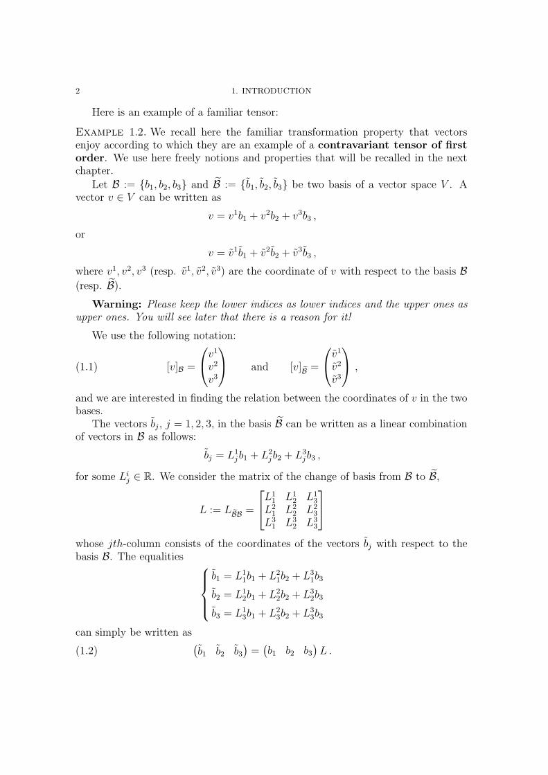
Example 1.2. We recall here the familiar transformation property that vectorsenjoy according to which they are an example of a contravariant tensor of firstorder. We use here freely notions and properties that will be recalled in the nextchapter.
Let B := {b1, b2, b3} and B := {b1, b2, b3} be two basis of a vector space V . Avector v ∈ V can be written as
v = v1b1 + v2b2 + v3b3 ,
or
v = v1b1 + v2b2 + v3b3 ,
where v1, v2, v3 (resp. v1, v2, v3) are the coordinate of v with respect to the basis B(resp. B).
Warning: Please keep the lower indices as lower indices and the upper ones as
upper ones. You will see later that there is a reason for it!
We use the following notation:
[v]B =
v1
v2
v3
and [v]B =
v1
v2
v3
,(1.1)
and we are interested in finding the relation between the coordinates of v in the twobases.
The vectors bj , j = 1, 2, 3, in the basis B can be written as a linear combinationof vectors in B as follows:
bj = L1jb1 + L2
jb2 + L3jb3 ,
for some Lij ∈ R. We consider the matrix of the change of basis from B to B,
L := LBB =
L11 L1
2 L13
L21 L2
2 L23
L31 L3
2 L33
whose jth-column consists of the coordinates of the vectors bj with respect to thebasis B. The equalities
b1 = L11b1 + L2
1b2 + L31b3
b2 = L12b1 + L2
2b2 + L32b3
b3 = L13b1 + L2
3b2 + L33b3
can simply be written as(b1 b2 b3
)=(b1 b2 b3
)L .(1.2)

1. INTRODUCTION 3
(Check this symbolic equation using the rules of matrix multiplication.) Analo-gously, writing basis vectors in a row and vector coordinates in a column, we canwrite
v = v1b1 + v2b2 + v3b3 =(b1 b2 b3
)v1
v2
v3
(1.3)
and
v = v1b1 + v2b2 + v3b3 =(b1 b2 b3
)v1
v2
v3
=
(b1 b2 b3
)L
v1
v2
v3
,(1.4)
where we used (1.2) in the last equality. Comparing the expression of v in (1.3) andin (1.4), we conclude that
L
v1
v2
v3
=
v1
v2
v3
or equivalently
v1
v2
v3
= L−1
v1
v2
v3
We say that the components of a vector v are contravariant1 because they changeby L−1 when the basis changes by L. A vector v is hence a contravariant 1-tensoror tensor of order (1, 0). �
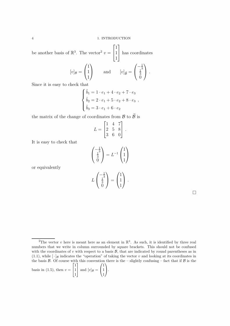
Example 1.3 (A numerical example). Let
B = {e1, e2, e3} =
100
,
010
,
001
(1.5)
be the standard basis or R3 and let
B = {b1, b2, b3} =
123
,
456
,
780
1In Latin contra means “contrary’, against”.
4 1. INTRODUCTION
be another basis of R3. The vector2 v =
111
has coordinates
[v]B =
111
and [v]B =
−1
3130
.
Since it is easy to check that
b1 = 1 · e1 + 4 · e2 + 7 · e3b2 = 2 · e1 + 5 · e2 + 8 · e3b3 = 3 · e1 + 6 · e2
,
the matrix of the change of coordinates from B to B is
L =
1 4 72 5 83 6 0
.
It is easy to check that−1
3130
= L−1
111
or equivalently
L
−1
3130
=
111
.
�
2The vector v here is meant here as an element in R3. As such, it is identified by three real
numbers that we write in column surrounded by square brackets. This should not be confusedwith the coordinates of v with respect to a basis B, that are indicated by round parentheses as in(1.1), while [ · ]B indicates the “operation” of taking the vector v and looking at its coordinates inthe basis B. Of course with this convention there is the – slightly confusing – fact that if B is the
basis in (1.5), then v =
111
and [v]B =
111
.

CHAPTER 2
Review of Linear Algebra
2.1. Vector Spaces and Subspaces
Definition 2.1. A vector space V over R is a set V equipped with two operations:
(1) Vector addition: V × V → V , (v, w) 7→ v + w, and(2) Multiplication by a scalar: R× V → V , (α, v) 7→ αv ,
satisfying the following properties:
(1) (associativity) (u+ v) + w = u+ (v + w) for every u, v, w ∈ V ;(2) (commutativity) u+ v = v + u for every u, v ∈ V ;(3) (existence of the zero vector) there exists 0 ∈ V such that v + 0 = v for
every v ∈ V ;(4) (existence of additive inverse) For every v ∈ V , there exists wv ∈ V such
that v + wv = 0. The vector wv is denoted by −v.(5) α(βv) = (αβ)v for every α, β ∈ R and every v ∈ R;(6) 1v = v for every v ∈ V ;(7) α(u+ w) = αu+ αv for all α ∈ R and u, v ∈ V ;(8) (α + β)v = αu+ βv for all α, β ∈ R and v ∈ V .
An element of the vector space is called a vector.
Example 2.2 (Prototypical example). The Euclidean space Rn, n = 1, 2, 3, . . . , is
a vector space with componentwise addition and multiplication by scalars. Vectors
in Rn are denoted by v =
x1...xn
, with x1, . . . , xn ∈ R. �
Examples 2.3 (Other examples). (1) The set of real polynomials of degree ≤n is a vector space, denoted by
V = R[x]n := {a0xn + a1xn−1 + · · ·+ an−1x+ an : aj ∈ R} .
(2) The set of real matrices of size m× n,
V =Mm×n(R) :=
a11 . . . a1m...
...an1 . . . anm
: aij ∈ R
.
(3) The space of solutions of a homogeneous linear (ordinary or partial) differ-ential equation.
5
6 2. REVIEW OF LINEAR ALGEBRA
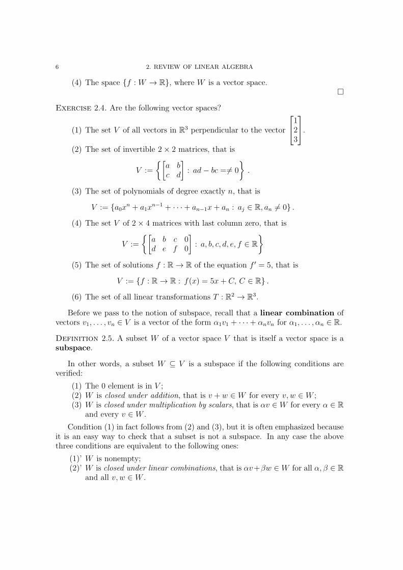
(4) The space {f : W → R}, where W is a vector space.�
Exercise 2.4. Are the following vector spaces?
(1) The set V of all vectors in R3 perpendicular to the vector
123
.
(2) The set of invertible 2× 2 matrices, that is
V :=
{[a bc d
]: ad− bc = 6= 0
}.
(3) The set of polynomials of degree exactly n, that is
V := {a0xn + a1xn−1 + · · ·+ an−1x+ an : aj ∈ R, an 6= 0} .
(4) The set V of 2× 4 matrices with last column zero, that is
V :=
{[a b c 0d e f 0
]: a, b, c, d, e, f ∈ R
}
(5) The set of solutions f : R→ R of the equation f ′ = 5, that is
V := {f : R→ R : f(x) = 5x+ C, C ∈ R} .
(6) The set of all linear transformations T : R2 → R3.
Before we pass to the notion of subspace, recall that a linear combination ofvectors v1, . . . , vn ∈ V is a vector of the form α1v1 + · · ·+ αnvn for α1, . . . , αn ∈ R.
Definition 2.5. A subset W of a vector space V that is itself a vector space is asubspace.
In other words, a subset W ⊆ V is a subspace if the following conditions areverified:
(1) The 0 element is in V ;(2) W is closed under addition, that is v + w ∈ W for every v, w ∈ W ;(3) W is closed under multiplication by scalars, that is αv ∈ W for every α ∈ R
and every v ∈ W .
Condition (1) in fact follows from (2) and (3), but it is often emphasized becauseit is an easy way to check that a subset is not a subspace. In any case the abovethree conditions are equivalent to the following ones:
(1)’ W is nonempty;(2)’ W is closed under linear combinations, that is αv+βw ∈ W for all α, β ∈ R
and all v, w ∈ W .
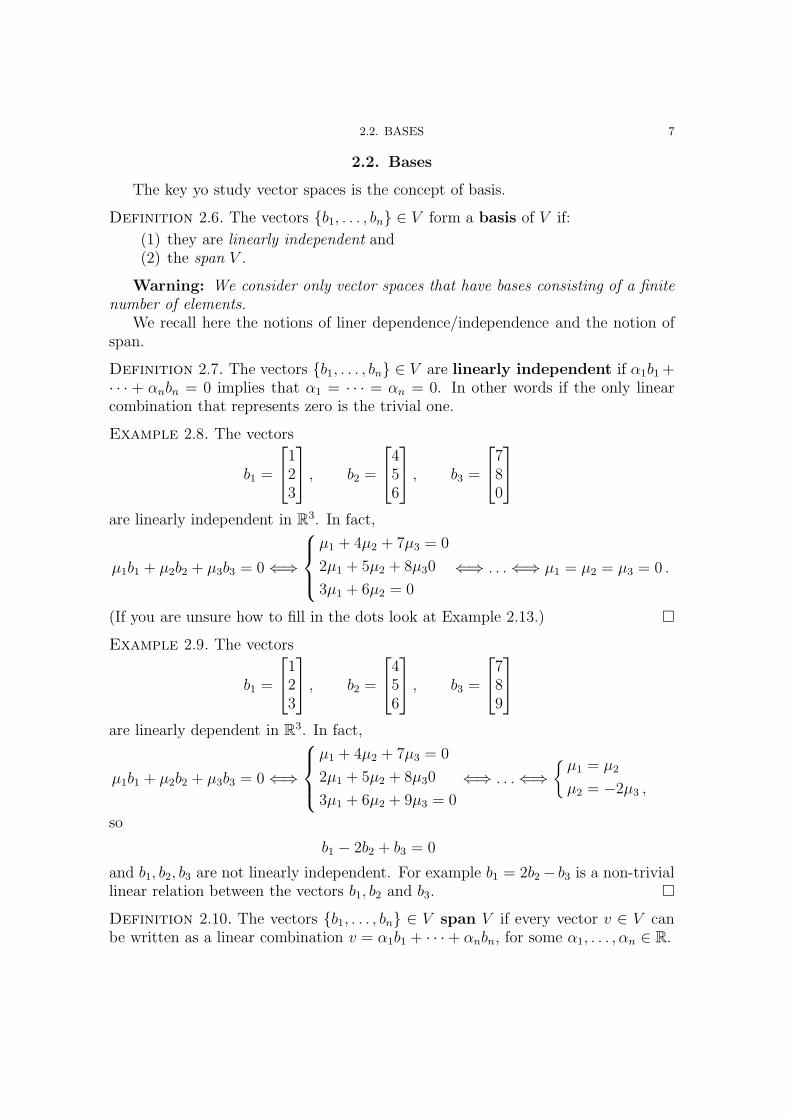
2.2. BASES 7
2.2. Bases
The key yo study vector spaces is the concept of basis.
Definition 2.6. The vectors {b1, . . . , bn} ∈ V form a basis of V if:
(1) they are linearly independent and(2) the span V .
Warning: We consider only vector spaces that have bases consisting of a finite
number of elements.
We recall here the notions of liner dependence/independence and the notion ofspan.
Definition 2.7. The vectors {b1, . . . , bn} ∈ V are linearly independent if α1b1+· · · + αnbn = 0 implies that α1 = · · · = αn = 0. In other words if the only linearcombination that represents zero is the trivial one.
Example 2.8. The vectors
b1 =
123
, b2 =
456
, b3 =
780
are linearly independent in R3. In fact,
µ1b1 + µ2b2 + µ3b3 = 0⇐⇒
µ1 + 4µ2 + 7µ3 = 0
2µ1 + 5µ2 + 8µ30
3µ1 + 6µ2 = 0
⇐⇒ . . .⇐⇒ µ1 = µ2 = µ3 = 0 .
(If you are unsure how to fill in the dots look at Example 2.13.) �
Example 2.9. The vectors
b1 =
123
, b2 =
456
, b3 =
789
are linearly dependent in R3. In fact,
µ1b1 + µ2b2 + µ3b3 = 0⇐⇒
µ1 + 4µ2 + 7µ3 = 0
2µ1 + 5µ2 + 8µ30
3µ1 + 6µ2 + 9µ3 = 0
⇐⇒ . . .⇐⇒{µ1 = µ2
µ2 = −2µ3 ,
so
b1 − 2b2 + b3 = 0
and b1, b2, b3 are not linearly independent. For example b1 = 2b2− b3 is a non-triviallinear relation between the vectors b1, b2 and b3. �
Definition 2.10. The vectors {b1, . . . , bn} ∈ V span V if every vector v ∈ V canbe written as a linear combination v = α1b1 + · · ·+ αnbn, for some α1, . . . , αn ∈ R.
8 2. REVIEW OF LINEAR ALGEBRA
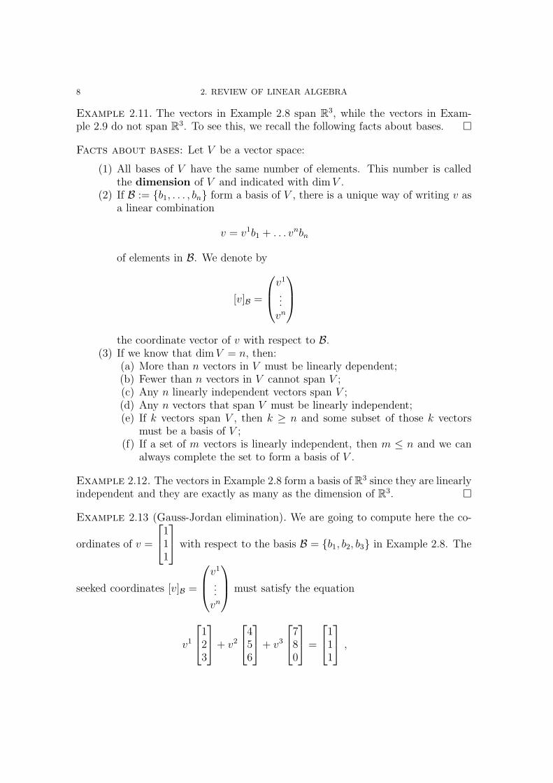
Example 2.11. The vectors in Example 2.8 span R3, while the vectors in Exam-
ple 2.9 do not span R3. To see this, we recall the following facts about bases. �
Facts about bases: Let V be a vector space:
(1) All bases of V have the same number of elements. This number is calledthe dimension of V and indicated with dimV .
(2) If B := {b1, . . . , bn} form a basis of V , there is a unique way of writing v asa linear combination
v = v1b1 + . . . vnbn
of elements in B. We denote by
[v]B =
v1
...vn
the coordinate vector of v with respect to B.(3) If we know that dimV = n, then:
(a) More than n vectors in V must be linearly dependent;(b) Fewer than n vectors in V cannot span V ;(c) Any n linearly independent vectors span V ;(d) Any n vectors that span V must be linearly independent;(e) If k vectors span V , then k ≥ n and some subset of those k vectors
must be a basis of V ;(f) If a set of m vectors is linearly independent, then m ≤ n and we can
always complete the set to form a basis of V .
Example 2.12. The vectors in Example 2.8 form a basis of R3 since they are linearlyindependent and they are exactly as many as the dimension of R3. �
Example 2.13 (Gauss-Jordan elimination). We are going to compute here the co-
ordinates of v =
111
with respect to the basis B = {b1, b2, b3} in Example 2.8. The
seeked coordinates [v]B =
v1
...vn
must satisfy the equation
v1
123
+ v2
456
+ v3
780
=
111
,
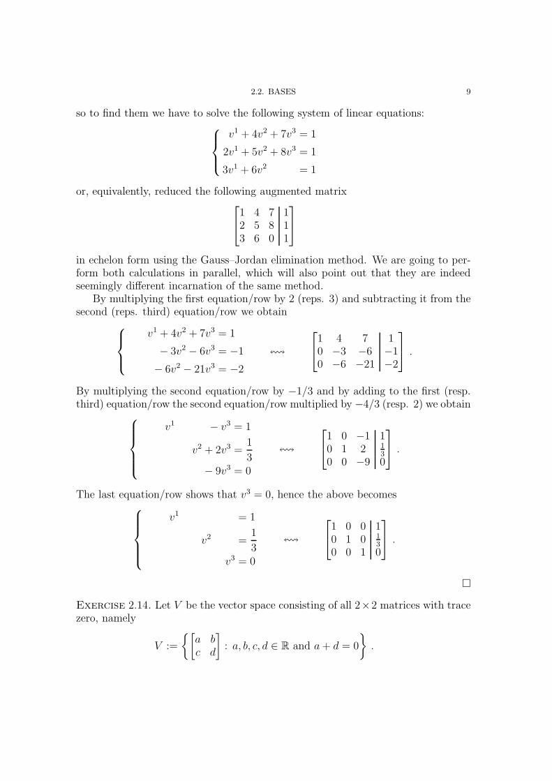
2.2. BASES 9
so to find them we have to solve the following system of linear equations:
v1 + 4v2 + 7v3 = 1
2v1 + 5v2 + 8v3 = 1
3v1 + 6v2 = 1
or, equivalently, reduced the following augmented matrix1 4 7 12 5 8 13 6 0 1
in echelon form using the Gauss–Jordan elimination method. We are going to per-form both calculations in parallel, which will also point out that they are indeedseemingly different incarnation of the same method.
By multiplying the first equation/row by 2 (reps. 3) and subtracting it from thesecond (reps. third) equation/row we obtain
v1 + 4v2 + 7v3 = 1
− 3v2 − 6v3 = −1− 6v2 − 21v3 = −2
!
1 4 7 10 −3 −6 −10 −6 −21 −2
.
By multiplying the second equation/row by −1/3 and by adding to the first (resp.third) equation/row the second equation/row multiplied by −4/3 (resp. 2) we obtain
v1 − v3 = 1
v2 + 2v3 =1
3− 9v3 = 0
!
1 0 −1 10 1 2 1
30 0 −9 0
.
The last equation/row shows that v3 = 0, hence the above becomes
v1 = 1
v2 =1
3v3 = 0
!
1 0 0 10 1 0 1
30 0 1 0
.
�
Exercise 2.14. Let V be the vector space consisting of all 2×2 matrices with tracezero, namely
V :=
{[a bc d
]: a, b, c, d ∈ R and a+ d = 0
}.
10 2. REVIEW OF LINEAR ALGEBRA
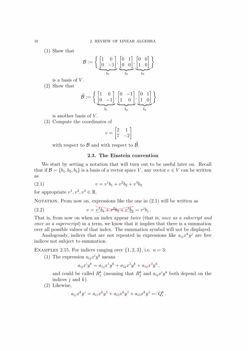
(1) Show that
B :=
{[1 00 −1
]
︸ ︷︷ ︸b1
,
[0 10 0
]
︸ ︷︷ ︸b2
,
[0 01 0
]
︸ ︷︷ ︸b3
}
is a basis of V .(2) Show that
B :=
{[1 00 −1
]
︸ ︷︷ ︸b1
,
[0 −11 0
]
︸ ︷︷ ︸b2
,
[0 11 0
]
︸ ︷︷ ︸b3
}
is another basis of V .(3) Compute the coordinates of
v =
[2 17 −2
]
with respect to B and with respect to B.
2.3. The Einstein convention
We start by setting a notation that will turn out to be useful later on. Recallthat if B = {b1, b2, b3} is a basis of a vector space V , any vector v ∈ V can be writtenas
v = v1b1 + v2b2 + v3b3(2.1)
for appropriate v1, v2, v3 ∈ R.
Notation. From now on, expressions like the one in (2.1) will be written as
v =✭✭
✭✭✭✭✭✭✭✭❤
❤❤❤❤❤❤❤❤❤
v1b1 + v2b2 + v3b3 = vjbj .(2.2)
That is, from now on when an index appear twice (that is, once as a subscript and
once as a superscript) in a term, we know that it implies that there is a summationover all possible values of that index. The summation symbol will not be displayed.
Analogously, indices that are not repeated in expressions like aijxkyj are free
indices not subject to summation.
Examples 2.15. For indices ranging over {1, 2, 3}, i.e. n = 3:
(1) The expression aijxiyk means
aijxiyk = a1jx
1yk + a2jx2yk + a3jx
3yk ,
and could be called Rkj (meaning that Rk
j and aijxiyk both depend on the
indices j and k).(2) Likewise,
aijxkyj = ai1x
ky1 + ai2xky2 + ai3x
ky3 =: Qki .
2.3. THE EINSTEIN CONVENTION 11
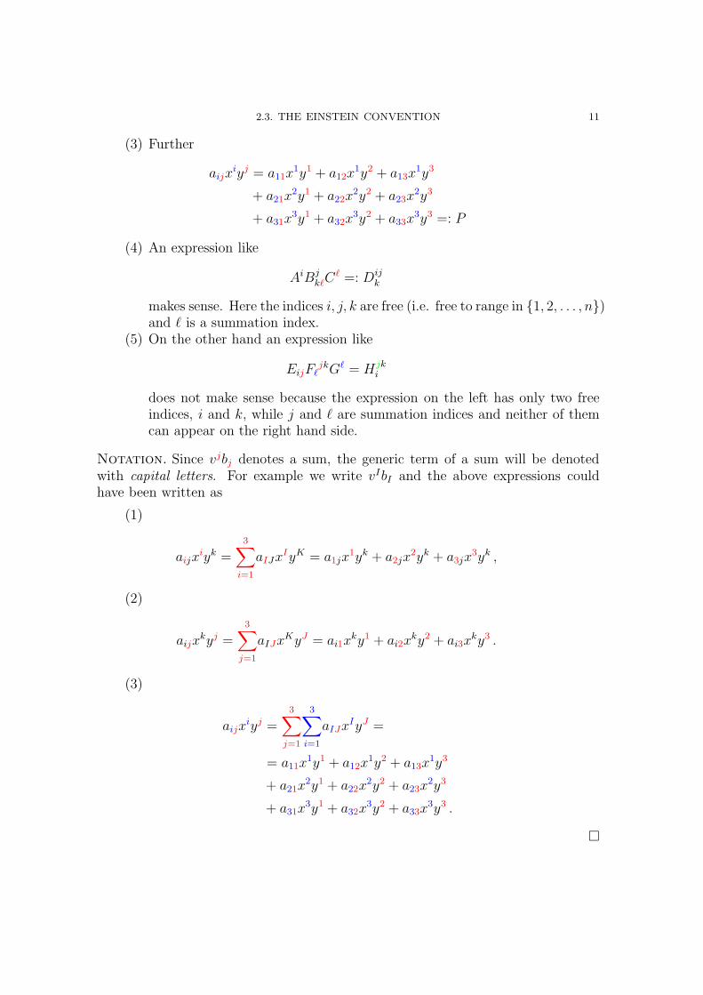
(3) Further
aijxiyj = a11x
1y1 + a12x1y2 + a13x
1y3
+ a21x2y1 + a22x
2y2 + a23x2y3
+ a31x3y1 + a32x
3y2 + a33x3y3 =: P
(4) An expression like
AiBjkℓC
ℓ =: Dijk
makes sense. Here the indices i, j, k are free (i.e. free to range in {1, 2, . . . , n})and ℓ is a summation index.
(5) On the other hand an expression like
EijFℓjkGℓ = Hjk
i
does not make sense because the expression on the left has only two freeindices, i and k, while j and ℓ are summation indices and neither of themcan appear on the right hand side.
Notation. Since vjbj denotes a sum, the generic term of a sum will be denotedwith capital letters. For example we write vIbI and the above expressions couldhave been written as
(1)
aijxiyk =
3∑
i=1
aIJxIyK = a1jx
1yk + a2jx2yk + a3jx
3yk ,
(2)
aijxkyj =
3∑
j=1
aIJxKyJ = ai1x
ky1 + ai2xky2 + ai3x
ky3 .
(3)
aijxiyj =
3∑
j=1
3∑
i=1
aIJxIyJ =
= a11x1y1 + a12x
1y2 + a13x1y3
+ a21x2y1 + a22x
2y2 + a23x2y3
+ a31x3y1 + a32x
3y2 + a33x3y3 .
�
12 2. REVIEW OF LINEAR ALGEBRA
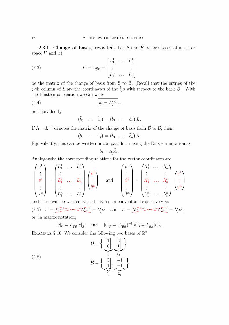
2.3.1. Change of bases, revisited. Let B and B be two bases of a vectorspace V and let
L := LBB =
L11 . . . L1
n...
...Ln1 . . . Ln
n
(2.3)
be the matrix of the change of basis from B to B. [Recall that the entries of the
j-th column of L are the coordinates of the bjs with respect to the basis B.] Withthe Einstein convention we can write
bj = Lijbi , .(2.4)
or, equivalently(b1 . . . bn
)=(b1 . . . bn
)L .
If Λ = L−1 denotes the matrix of the change of basis from B to B, then(b1 . . . bn
)=(b1 . . . bn
)Λ .
Equivalently, this can be written in compact form using the Einstein notation as
bj = Λij bi .
Analogously, the corresponding relations for the vector coordinates are
v1
...vi
...vn
=
L11 . . . L1
n...
...Li1 . . . Li
n...
...Ln1 . . . Ln
n
v1
...vn
and
v1
...vi
...vn
=
Λ11 . . . Λ1
n...
...Λi
1 . . . Λin
......
Λn1 . . . Λn
n
v1
...vn
and these can be written with the Einstein convention respectively as
vi =✭✭✭✭✭✭✭✭✭✭❤
❤❤❤❤❤❤❤❤❤
Li1v
1 + · · ·+ Linv
n = Lij v
j and vi =✭✭✭✭✭✭✭✭✭✭❤
❤❤❤❤❤❤❤❤❤
Λi1v
1 + · · ·+ Λinv
n = Λijv
j ,(2.5)
or, in matrix notation,
[v]B = LBB[v]B and [v]B = (LBB)−1[v]B = LBB[v]B .
Example 2.16. We consider the following two bases of R2
B =
{ [10
]
︸︷︷︸b1
,
[21
]
︸︷︷︸b2
}
B =
{ [31
]
︸︷︷︸b1
,
[−1−1
]
︸ ︷︷ ︸b2
}(2.6)

2.3. THE EINSTEIN CONVENTION 13
and we look for the matrix of the change of basis. Namely we look for a matrix Lsuch that [
3 −11 −1
]=(b1 b2
)=(b1 b2
)L =
[1 20 1
]L .
There are two alternative ways of finding L:
(1) With matrix inversion: Recall that[a bc d
]−1
=1
D
[d −b−c a
],(2.7)
where D = det
([a bc d
]). Thus
L =
[1 20 1
]−1 [3 −11 −1
]=
[1 −20 1
] [3 −11 −1
]=
[1 11 −1
].
(2) With the Gauss-Jordan elimination:[1 2 3 −10 1 1 −1
]!
[1 0 1 10 1 1 −1
]
�
2.3.2. The Kronecker delta symbol.
Notation. The Kronecker delta symbol δij is defined as
δij :=
{1 if i = j
0 if i 6= j .(2.8)
Examples 2.17. If L is a matrix, the (i, j)-entry of L is the coefficient in the i-throw and j-th column, and is denoted by Li
j .
(1) The n× n identity matrix
I =
1 . . . 0...
. . ....
0 . . . 1
has (i, j)-entry equal to δij .(2) Let L and Λ be two square matrices. The (i, j)-th entry of the product ΛL
ΛL =
Λ11 . . . Λ1
n...
...Λi
1 . . . Λin
......
Λn1 . . . Λn
n
L11 . . . L1
j . . . L1n
......
...Ln1 . . . Ln
j . . . Lnn

14 2. REVIEW OF LINEAR ALGEBRA
equals the dot product of the i-th row and j-th column,
(Λi
1 . . . Λin
)·
L1j...Lnj
= Λi
1L1j + · · ·+ Λi
nLnj ,
or, using the Einstein convention,
ΛikL
kj
Notice that since in general ΛL 6= LΛ, it follows that
ΛikL
kj 6= Li
kΛkj = Λk
jLik .
On the other hand, if Λ = L−1, that is ΛL = LΛ = I, then we can write
ΛikL
kj = δij = Li
kΛkj .
�
Remark 2.18. Using the Kronecker delta symbol we can check that the notationsin (2.5) are all consistent. In fact, from (2.2) we should have
vibi = v = vibi ,(2.9)
and, in fact, using (2.5),
vibi = Λijv
jLki bk = δkj v
jbk = vjbj ,
where we used that ΛijL
ki = δkj since Λ = L−1.
Two words of warning:
• The two expressions vjbj and vkbk are identical, as the indices j and k aredummy indices.• When multiplying two different expressions in Einstein notation, you shouldbe careful to distinguish by different letters different summation indices. Forexample, if vi = Λi
jvj and bi = Lj
i bj , in order to perform the multiplication
vibi we have to make sure to replace one of the dummy indices in thetwo expressions. So, for example, we can write bi = Lk
i bk, so that vibi =Λi
jvjLk
i bk.
2.4. Linear Transformations
Let T : V → V be a linear transformation, that is a transformation that satisfiesthe property
T (αv + βw) = αT (v) + βT (w) ,
for all α, β ∈ R and all v, w ∈ V . Once we choose a basis of V , the transformationT is represented by a matrix A with respect to that basis, and that matrix gives
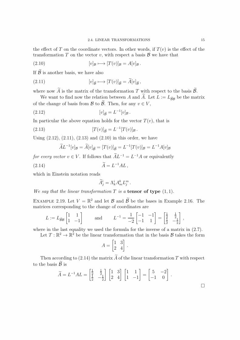
2.4. LINEAR TRANSFORMATIONS 15
the effect of T on the coordinate vectors. In other words, if T (v) is the effect of thetransformation T on the vector v, with respect a basis B we have that
[v]B 7−→ [T (v)]B = A[v]B .(2.10)
If B is another basis, we have also
[v]B 7−→ [T (v)]B = A[v]B ,(2.11)
where now A is the matrix of the transformation T with respect to the basis B.We want to find now the relation between A and A. Let L := LBB be the matrix
of the change of basis from B to B. Then, for any v ∈ V ,
[v]B = L−1[v]B .(2.12)
In particular the above equation holds for the vector T (v), that is
[T (v)]B = L−1[T (v)]B .(2.13)
Using (2.12), (2.11), (2.13) and (2.10) in this order, we have
AL−1[v]B = A[v]B = [T (v)]B = L−1[T (v)]B = L−1A[v]B
for every vector v ∈ V . If follows that AL−1 = L−1A or equivalently
A = L−1AL ,(2.14)
which in Einstein notation reads
Aij = Λi
kAkmL
mj .
We say that the linear transformation T is a tensor of type (1, 1).
Example 2.19. Let V = R2 and let B and B be the bases in Example 2.16. The
matrices corresponding to the change of coordinates are
L := LBB
[1 11 −1
]and L−1 =
1
−2
[−1 −1−1 1
]=
[12
12
12−1
2
],
where in the last equality we used the formula for the inverse of a matrix in (2.7).Let T : R2 → R
2 be the linear transformation that in the basis B takes the form
A =
[1 32 4
].
Then according to (2.14) the matrix A of the linear transformation T with respect
to the basis B is
A = L−1AL =
[12
12
12−1
2
] [1 32 4
] [1 11 −1
]=
[5 −2−1 0
].
�

16 2. REVIEW OF LINEAR ALGEBRA
Example 2.20. We now look for the standard matrix of T , that is the matrix Mthat represents T with respect to the standard basis of R2, which we denote by
E :=
{ [10
]
︸︷︷︸e1
,
[01
]
︸︷︷︸e2
}.
We want to apply again the formula (2.14) and hence we first need to find the matrixS := LBE of the change of basis from E to B. Recall that the columns of S are thecoordinates of bj with respect to the basis E , that is
S =
[1 20 1
].
According to (2.14),
A = S−1MS ,
from which, using again (2.7), we obtain
M = SAS−1 =
[1 20 1
] [1 32 4
] [1 −20 1
]=
[1 20 1
] [1 12 0
]=
[5 12 0
].
�
Example 2.21. Let T : R3 → R3 be the orthogonal projection onto the plane P of
equation
2x+ y − z = 0 .
This means that the transformation T is characterized by the fact that
– it does not change vectors in the plane P, and– it takes to zero vectors perpendicular to P.
We want to find the standard matrix for T .
Idea: First compute the matrix of T with respect to a basis B of R3 well adaptedto the problem, then use (2.14) after having found the matrix LBE of the change ofbasis.
To this purpose, we choose two linearly independent vectors in the plane P anda third vector perpendicular to P. For instance, we set
B :=
{102
︸︷︷︸b1
,
011
︸︷︷︸b2
,
21−1
︸ ︷︷ ︸b3
},
where the coordinates of b1 and b2 satisfy the equation of the plane, while thecoordinates of b3 are the coefficients of the equation describing P. Let E be thestandard basis of R3.
2.4. LINEAR TRANSFORMATIONS 17
Since
T (b1) = b1, T (b2) = b2 and T (b3) = 0 ,
the matrix of T with respect to B is
A =
1 0 00 1 00 0 0
,(2.15)
where we recall that the j-th column are the coordinates [T (bj)]B of the vector T (bj)with respect to the basis B.
The matrix of the change of basis from E to B is
L =
1 0 20 1 12 1 −1
,
hence, by Gauss–Jordan elimination,
L−1 =
13−1
313
−13
56
16
13
16−1
6
.
Therefore
M = LAL−1 = · · · =
13−1
313
−13
56
16
13
16
56
.
�
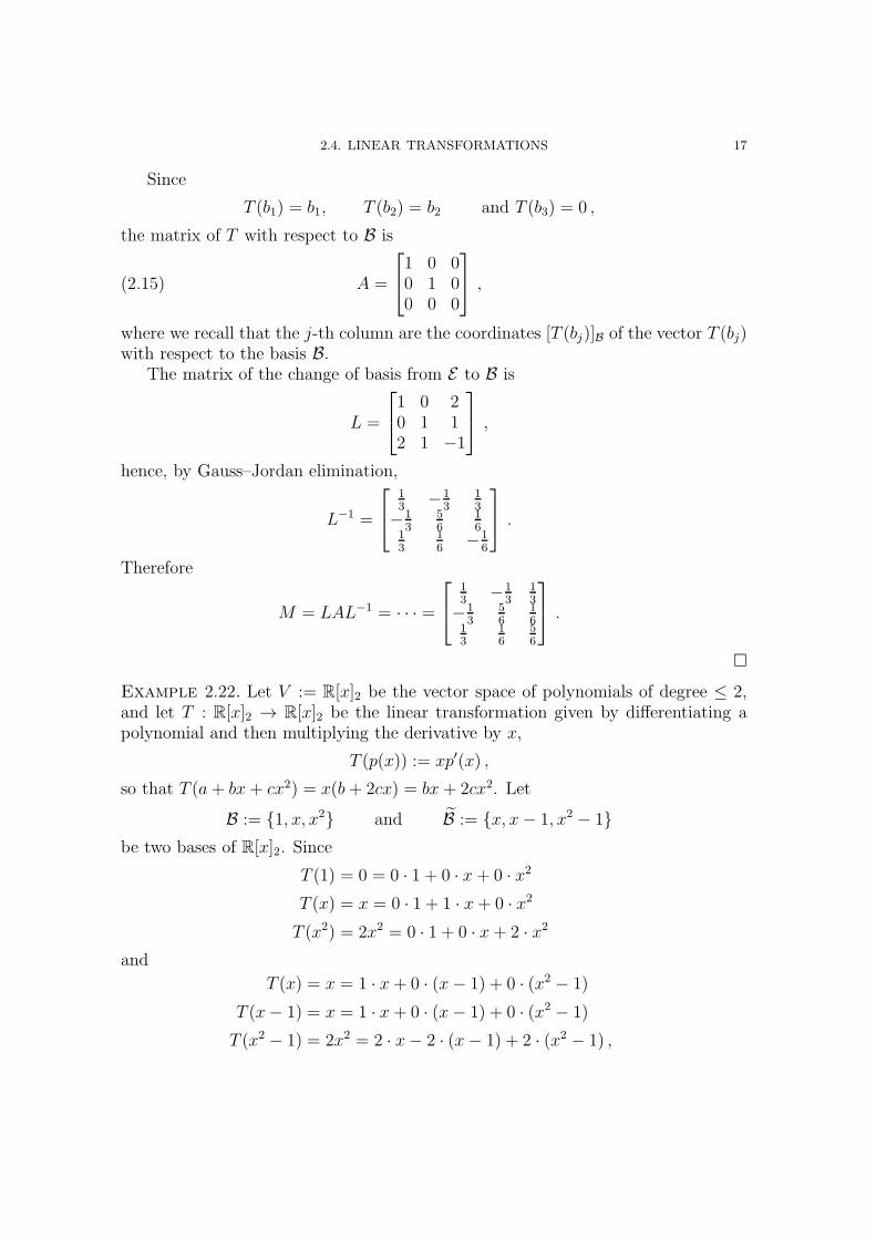
Example 2.22. Let V := R[x]2 be the vector space of polynomials of degree ≤ 2,and let T : R[x]2 → R[x]2 be the linear transformation given by differentiating apolynomial and then multiplying the derivative by x,
T (p(x)) := xp′(x) ,
so that T (a+ bx+ cx2) = x(b+ 2cx) = bx+ 2cx2. Let
B := {1, x, x2} and B := {x, x− 1, x2 − 1}be two bases of R[x]2. Since
T (1) = 0 = 0 · 1 + 0 · x+ 0 · x2
T (x) = x = 0 · 1 + 1 · x+ 0 · x2
T (x2) = 2x2 = 0 · 1 + 0 · x+ 2 · x2
and
T (x) = x = 1 · x+ 0 · (x− 1) + 0 · (x2 − 1)
T (x− 1) = x = 1 · x+ 0 · (x− 1) + 0 · (x2 − 1)
T (x2 − 1) = 2x2 = 2 · x− 2 · (x− 1) + 2 · (x2 − 1) ,
18 2. REVIEW OF LINEAR ALGEBRA
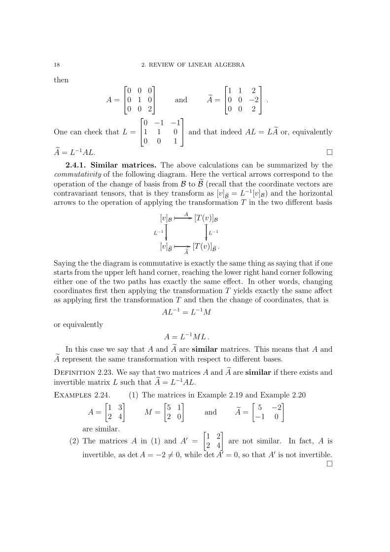
then
A =
0 0 00 1 00 0 2
and A =
1 1 20 0 −20 0 2
.
One can check that L =
0 −1 −11 1 00 0 1
and that indeed AL = LA or, equivalently
A = L−1AL. �
2.4.1. Similar matrices. The above calculations can be summarized by thecommutativity of the following diagram. Here the vertical arrows correspond to the
operation of the change of basis from B to B (recall that the coordinate vectors arecontravariant tensors, that is they transform as [v]B = L−1[v]B) and the horizontalarrows to the operation of applying the transformation T in the two different basis
[v]B✤ A
//❴
L−1
��
[T (v)]B❴
L−1
��
[v]B✤
A
// [T (v)]B .
Saying the the diagram is commutative is exactly the same thing as saying that if onestarts from the upper left hand corner, reaching the lower right hand corner followingeither one of the two paths has exactly the same effect. In other words, changingcoordinates first then applying the transformation T yields exactly the same affectas applying first the transformation T and then the change of coordinates, that is
AL−1 = L−1M
or equivalently
A = L−1ML .
In this case we say that A and A are similar matrices. This means that A and
A represent the same transformation with respect to different bases.
Definition 2.23. We say that two matrices A and A are similar if there exists and
invertible matrix L such that A = L−1AL.
Examples 2.24. (1) The matrices in Example 2.19 and Example 2.20
A =
[1 32 4
]M =
[5 12 0
]and A =
[5 −2−1 0
]
are similar.
(2) The matrices A in (1) and A′ =
[1 22 4
]are not similar. In fact, A is
invertible, as detA = −2 6= 0, while detA′ = 0, so that A′ is not invertible.�

2.5. EIGENBASES 19
We collect here few facts about similar matrices. Recall that the eigenvaluesof a matrix A are the roots of the characteristic polynomial
pA(λ) := det(A− λI) .Moreover
(1) the determinant of a matrix is the product of its eigenvalues, and(2) the trace of a matrix is the sum of its eigenvalues.
Let us assume that A and A are similar matrices, that is A = L−1AL for someinvertible matrix L. Then
pA(λ) = det(A− λI) = det(L−1AL− λL−1IL)
= det(L−1(A− λI)L)=
✘✘✘✘✘
(detL−1) det(A− λI)✘✘✘✘(detL) = pA(λ) ,
(2.16)
which means that any two similar matrices have the same characteristic polynomial.
Facts about similar matrices: From (2.16) if follows immediately that if the
matrices A and A are similar, then:
• A and A have the same size;• the eigenvalues of A (as well as their multiplicity) are the same as those of
A;• detA = det A;
• trA = tr A;
• A is invertible if and only if A is invertible.
2.5. Eigenbases
The possibility of choosing different bases is very important and often simplifiesthe calculations. Example 2.21 is such an example, where we choose an appropriatebasis according to the specific problem. Other times a basis can be chosen accordingto the symmetries and, completely at the opposite side, sometime there is just nota basis that is a preferred one. One basis that is particularly important, when itexists, is an eigenbasis with respect to some linear transformation A of V .
Recall that an eigenvector of a linear transformation A corresponding to aneigenvalue λ is a non-zero vector v ∈ Eλ := ker(A − λI). An eigenbasis of avector space V is a basis consisting of eigenvectors of a linear transformation A ofV . The point of having an eigenbasis is that, with respect to this eigenbasis, thelinear transformation is as simple as possible, that is is as close as possible to bediagonal. This diagonal matrix similar to A is called the Jordan canonical formof A.
Given a linear transformation T : V → V , in order to find an eigenbasis of T ,we need to perform the following steps:
(1) Compute the eigenvalues(2) Compute the eigenspaces
20 2. REVIEW OF LINEAR ALGEBRA
(3) Find a eigenbasis.
We will do this in the following example.
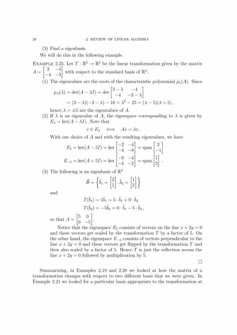
Example 2.25. Let T : R2 → R2 be the linear transformation given by the matrix
A =
[3 −4−4 −3
]with respect to the standard basis of R2.
(1) The eigenvalues are the roots of the characteristic polynomial pλ(A). Since
pA(λ) = det(A− λI) = det
[3− λ −4−4 −3 − λ
]
= (3− λ)(−3− λ)− 16 = λ2 − 25 = (λ− 5)(λ+ 5) ,
hence λ = ±5 are the eigenvalues of A.(2) If λ is an eigenvalue of A, the eigenspace corresponding to λ is given by
Eλ = ker(A− λI). Note that
v ∈ Eλ ⇐⇒ Av = λv .
With our choice of A and with the resulting eigenvalues, we have
E5 = ker(A− 5I) = ker
[−2 −4−4 −8
]= span
[2−1
]
E−5 = ker(A+ 5I) = ker
[−8 −4−4 −2
]= span
[12
].
(3) The following is an eigenbasis of R2
B =
{b1 =
[21
], b2 =
[12
]}
and
T (b1) = 5b1 = 5 · b1 + 0 · b2T (b2) = −5b2 = 0 · b1 − 5 · b2 ,
so that A =
[5 00 −5
].
Notice that the eigenspace E5 consists of vectors on the line x+ 2y = 0and these vectors get scaled by the transformation T by a factor of 5. Onthe other hand, the eigenspace E−5 consists of vectors perpendicular to theline x + 2y = 0 and these vectors get flipped by the transformation T andthen also scaled by a factor of 5. Hence T is just the reflection across theline x+ 2y = 0 followed by multiplication by 5.
�
Summarizing, in Examples 2.19 and 2.20 we looked at how the matrix of atransformation changes with respect to two different basis that we were given. InExample 2.21 we looked for a particular basis appropriate to the transformation at

2.5. EIGENBASES 21
hand. In Example 2.25 we looked for an eigenbasis with respect to the given transfor-mation. Example 2.21 in this respect fits into the same framework as Example 2.25,but the orthogonal projection has a zero eigenvalue (see (2.15)).

CHAPTER 3
Multilinear Forms
3.1. Linear Forms
3.1.1. Definition, Examples, Dual and Dual Basis.
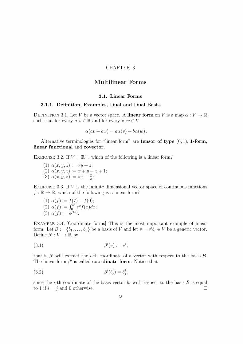
Definition 3.1. Let V be a vector space. A linear form on V is a map α : V → R
such that for every a, b ∈ R and for every v, w ∈ V
α(av + bw) = aα(v) + bα(w) .
Alternative terminologies for “linear form” are tensor of type (0, 1), 1-form,linear functional and covector.
Exercise 3.2. If V = R3 , which of the following is a linear form?
(1) α(x, y, z) := xy + z;(2) α(x, y, z) := x+ y + z + 1;(3) α(x, y, z) := πx− 7
2z.
Exercise 3.3. If V is the infinite dimensional vector space of continuous functionsf : R→ R, which of the following is a linear form?
(1) α(f) := f(7)− f(0);(2) α(f) :=
∫ 33
0exf(x)dx;
(3) α(f) := ef(x).
Example 3.4. [Coordinate forms] This is the most important example of linearform. Let B := {b1, . . . , bn} be a basis of V and let v = vibi ∈ V be a generic vector.Define βi : V → R by
βi(v) := vi ,(3.1)
that is βi will extract the i-th coordinate of a vector with respect to the basis B.The linear form βi is called coordinate form. Notice that
βi(bj) = δij ,(3.2)
since the i-th coordinate of the basis vector bj with respect to the basis B is equalto 1 if i = j and 0 otherwise. �
23

24 3. MULTILINEAR FORMS
Example 3.5. Let V = R3 and let E be its standard basis. The three coordinate
forms are defined by
β1
xyz
:= x , β2
xyz
:= y , β3
xyz
:= z .
�
Example 3.6. Let V = R2 and let B :=
{ [11
]
︸︷︷︸b1
,
[1−1
]
︸ ︷︷ ︸b2
}. We want to describe the
elements of B∗ := {β1, β2}, in other words we want to find
β1(v) and β2(v)
for a generic vector v ∈ V .To this purpose we need to find [v]B. Recall that if E denotes the standard basis
of R2 and L := LBE the matrix of the change of coordinate from E to B, then
[v]B = L−1[v]E = L−1
(v1
v2
).
Since
L =
[1 11 −1
]
and hence
L−1 =1
2
[1 11 −1
],
then
[v]B =
(12(v1 + v2)
12(v1 − v2)
).
Thus, according to (3.1), we deduce that
β1(v) =1
2(v1 + v2) and β2(v) =
1
2(v1 − v2) .
�
Let us define
V ∗ := {all linear forms α : V → R} .Exercise 3.7. Check that V ∗ is a vector space whose null vector is the linear formidentically equal to zero.
We called V ∗ the dual of V .

3.1. LINEAR FORMS 25
Proposition 3.8. Let B := {b1, . . . , bn} be a basis of V and β1, . . . , βn are thecorresponding coordinate forms. Then B∗ := {β1, . . . , βn} is a basis of V ∗. As aconsequence
dimV = dimV ∗ .
Proof. According to Definition 2.6 , we need to check that the linear forms inB∗
(1) span V and(2) are linearly independent.
(1) To check that B∗ spans V we need to verify that any α ∈ V ∗ is a linear combi-nation of β1, . . . , βn, that is that
α = αiβi(3.3)
for some αi ∈ R. Because of (3.2), if we apply both sides of (3.3) to the j-th basisvector bi, we obtain
α(bj) = αiβi(bj) = αiδ
ij = αj ,(3.4)
which identifies the coefficients in (3.3).Now let v = vibi ∈ V be an arbitrary vector. Then
α(v) = α(vibi) = viα(bi) = viαi ,
where the second equality follows form the definition of linear form and the thirdfrom (3.4).
On the other hand
αiβi(v) = αiβ
i(vjbj) = αivjβi(bj) = αiv
jδij = αivi .
Thus (3.3) is verified.
(2) We need to check that the only linear combination of β1, . . . , βn that givesthe zero linear form is the trivial linear combination. Let ciβ
i = 0 be a linearcombination of the βi. Then for every basis vector bj , with j = 1, . . . , n,
0 = (ciβi)(bj) = ci(β
i(bj)) = ciδij = cj ,
thus showing the linear independence. �
The basis B∗ of V ∗ is called the basis of V dual to B. We emphasize that thecoordinates (or components) of a linear form α with respect to B∗ are exactly thevalues of α on the elements of B,
αi = α(bi) .
Example 3.9. Let V = R[x]2 be the vector space of polynomials of degree ≤ 2, letα : V → R be the linear form given by
α(p(x)) := p(2)− p′(2)(3.5)
and let B := {1, x, x2} be a basis of V . We want to:
26 3. MULTILINEAR FORMS
(1) find the components of α with respect to B∗;(2) describe the basis B∗ = {β1, β2, β3};
(1) Since
α1 = α(b1) = α(1) = 1− 0 = 1
α2 = α(b2) = α(x) = 2− 1 = 1
α3 = α(b3) = α(x2) = 4− 4 = 0 ,
then
[α]B∗ =(1 1 0
).(3.6)
(2) The generic element p(x) ∈ R[x]2 written as combination of basis elements 1, xand x2 is
p(x) = a+ bx+ cx2 .
Hence B∗ = {β1, β2, β3}, is given by
β1(a+ bx+ cx2) = a
β2(a+ bx+ cx2) = b
β3(a+ bx+ cx2) = c .
(3.7)
�
Remark 3.10. Note that it does not make sense to talk about a “dual basis” of V ∗,as for every basis B of V there is going to be a basis B∗ of V ∗ dual to the basis B.In the next section we are going to see how the dual basis transform with a changeof basis.
3.1.2. Transformation of Linear Forms under a Change of Basis. Wewant to study how a linear form α : V → R behaves with respect to a change abasis in V . To this purpose, let
B := {b1, . . . , bn} and B := {b1, . . . , bn}be two bases of V and let
B∗ := {β1, . . . , βn} and B∗ := {β1, . . . , βn}the corresponding dual bases. Let
[α]B∗ =(α1 . . . αn
)and [α]B∗ =
(α1 . . . αn
)
be the coordinate vectors of α with respect to B∗ and B∗, that is
α(bi) = αi and α(bi) = αi .
Let L := LBB be the matrix of the change of basis in (2.3)
bj = Lijbi .

3.1. LINEAR FORMS 27
Then
αj = α(bj) = α(Lijbi) = Li
jα(bi) = Lijαi = αiL
ij ,(3.8)
so that
αj = αiLij .(3.9)
Exercise 3.11. Verify that (3.9) is equivalent to saying that
[α]B∗ = [α]B∗L .(3.10)
Note that we have exchanged the order of αi and Lij in the last equation in (3.8) to
respect the order in which the matrix multiplication in (3.10) has to be performed.This was possible because both αi and L
ij are real numbers.
We say that the component of a linear form α are covariant1 because theychange by L when the basis changes by L. A linear form α is hence a covarianttensor or a tensor of type (1, 0).
Example 3.12. We continue with Example 3.9. We consider the bases as in Exam-ple 2.22, that is
B := {1, x, x2} and B := {x, x− 1, x2 − 1}and the linear form α : V → R as in (3.5). We will:
(1) find the components of α with respect to B∗;(2) describe the basis B∗ = {β1, β2, β3};(3) find the components of α with respect to B∗;
(4) describe the basis B∗ = {β1, β2, β3};(5) find the matrix of change of basis L := LBB and compute Λ = L−1;(6) check the covariance of α;(7) check the contravariance of B∗.
(1) This is done in (3.6).
(2) This is done in (3.7).
(3) We proceed as in (3.6). Namely,
α1 = α(b1) = α(x) = 2− 1 = 1
α2 = α(b2) = α(x− 1) = 1− 1 = 0
α3 = α(b3) = α(x2 − 1) = 3− 4 = −1 ,so that
[α]B∗ =(1 −1 −1
).
1“co” is a prefix that in Latin means “joint”.
28 3. MULTILINEAR FORMS
(4) Since βi(v) = vi, to proceed as in (3.7) we first need to write the generic polyno-
mial p(x) = a + bx+ cx2 as a linear combination of elements in B, namely we need
to find a, b and c such that
p(x) = a+ bx+ cx2 = ax+ b(x− 1) + c(x2 − 1) .
By multiplying and collecting the terms, we obtain that
− b− c = a
a+ b = b
c = c
that is
a = a+ b+ c
b = −a− cc = c .
Hence
p(x) = a + bx+ cx2 = (a+ b+ c)x+ (−a− c)(x− 1) + c(x2 − 1) ,
so that it follows that
β1(p(x)) = a + b+ c
β2(p(x)) = −a− cβ3(p(x)) = c ,
(5) The matrix of the change of bases is given by
L := LBB =
0 −1 −11 1 00 0 1
,
since for example b3 can be written as a linear combination with respect to B asb3 = x2 − 1 = −1b1 + 0b2 + 1b3, and hence its coordinates form the third column ofL.
To compute Λ = L−1 we can use the Gauss–Jordan elimination process
0 −1 −1 1 0 01 1 0 0 1 00 0 1 0 0 1
! . . . !
1 0 0 1 1 10 1 0 −1 0 −10 0 1 0 0 1
Hence
Λ =
1 1 1−1 0 −10 0 1
(6) The linear form α is covariant since
(α1 α2 α3
)=(1 0 −1
)=(1 1 0
)0 −1 −11 1 00 0 1
=
(α1 α2 α3
)L
(7) The dual basis B∗ is contravariant since

3.1. LINEAR FORMS 29
Table 1. Covariance and Contravariance
The covariance The contravariaceof a tensor of a tensor
is characterized by lower indices upper indicesvectors are indicated as row vectors column vectorsthe tensor transforms w.r.t.
a change of basis B → B bymultiplication by L on the right L−1 on the left(for later use) if a tensoris of type (p, q) (p, q) (p, q)
β1
β2
β3
= Λ
β1
β2
β3
,
as it can be verified by looking at an arbitrary vector p(x) = a+ bx+ cx2
a + b+ c−a− cc
=
1 1 1−1 0 −10 0 1
abc
.
�
In fact, the statement in Example 3.9(7) holds in general, namely:
Claim 3.13. Dual bases are contravariant.
Proof. We will check that when bases B and B are related by
bj = Lijbi
the corresponding dual bases B∗ and B∗ of V ∗ are related by
βj = Λjiβ
i .(3.11)
It is enough to check that the Λjiβ
i are dual of the Lijbi. In fact, since ΛL = I, then
(Λkℓβ
ℓ)(Lijbi) = Λk
ℓLijβ
ℓ(bi) = ΛkℓL
ijδ
ℓi = Λk
iLij = δkj = βj(bj) .
�
In Table 1 you will find a summary of the properties that characterize covarianceand contravariance, while in Table 2 you can find a summary of the properties thatbases and dual bases, coordinate vectors and coordinates of linear forms satisfywith respect to a change of coordinates and hence whether they are covariant orcontravariant.
30 3. MULTILINEAR FORMS
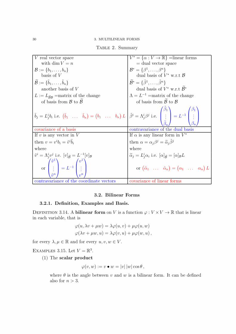
Table 2. Summary
V real vector space V ∗ = {α : V → R} =linear formswith dimV = n = dual vector space
B := {b1, . . . , bn} B∗ = {β1, . . . , βn}basis of V dual basis of V ∗ w.r.t B
B := {b1, . . . , bn} B∗ = {β1, . . . , βn}another basis of V dual basis of V ∗ w.r.t B∗
L := LBB =matrix of the change Λ = L−1 =matrix of the change
of basis from B to B of basis from B to B
bj = Lijbi i.e.
(b1 . . . bn
)=(b1 . . . bn
)L βi = Λi
jβj i.e.
β1...
βn
= L−1
β1...βn
covariance of a basis contravariance of the dual basisIf v is any vector in V If α is any linear form in V ∗
then v = vibi = vibi then α = αjβj = αjβ
j
where where
vi = Λijv
j i.e. [v]B = L−1[v]B αj = Lijαi i.e. [α]B = [α]BL
or
v1
...vn
= L−1
v1
...vn
or
(α1 . . . αn
)=(α1 . . . αn
)L
contravariance of the coordinate vectors covariance of linear forms
3.2. Bilinear Forms
3.2.1. Definition, Examples and Basis.
Definition 3.14. A bilinear form on V is a function ϕ : V ×V → R that is linearin each variable, that is
ϕ(u, λv + µw) = λϕ(u, v) + µϕ(u, w)
ϕ(λv + µw, u) = λϕ(v, u) + µϕ(w, u) ,
for every λ, µ ∈ R and for every u, v, w ∈ V .
Examples 3.15. Let V = R3.
(1) The scalar product
ϕ(v, w) := v • w = |v| |w| cos θ ,where θ is the angle between v and w is a bilinear form. It can be definedalso for n > 3.
3.2. BILINEAR FORMS 31
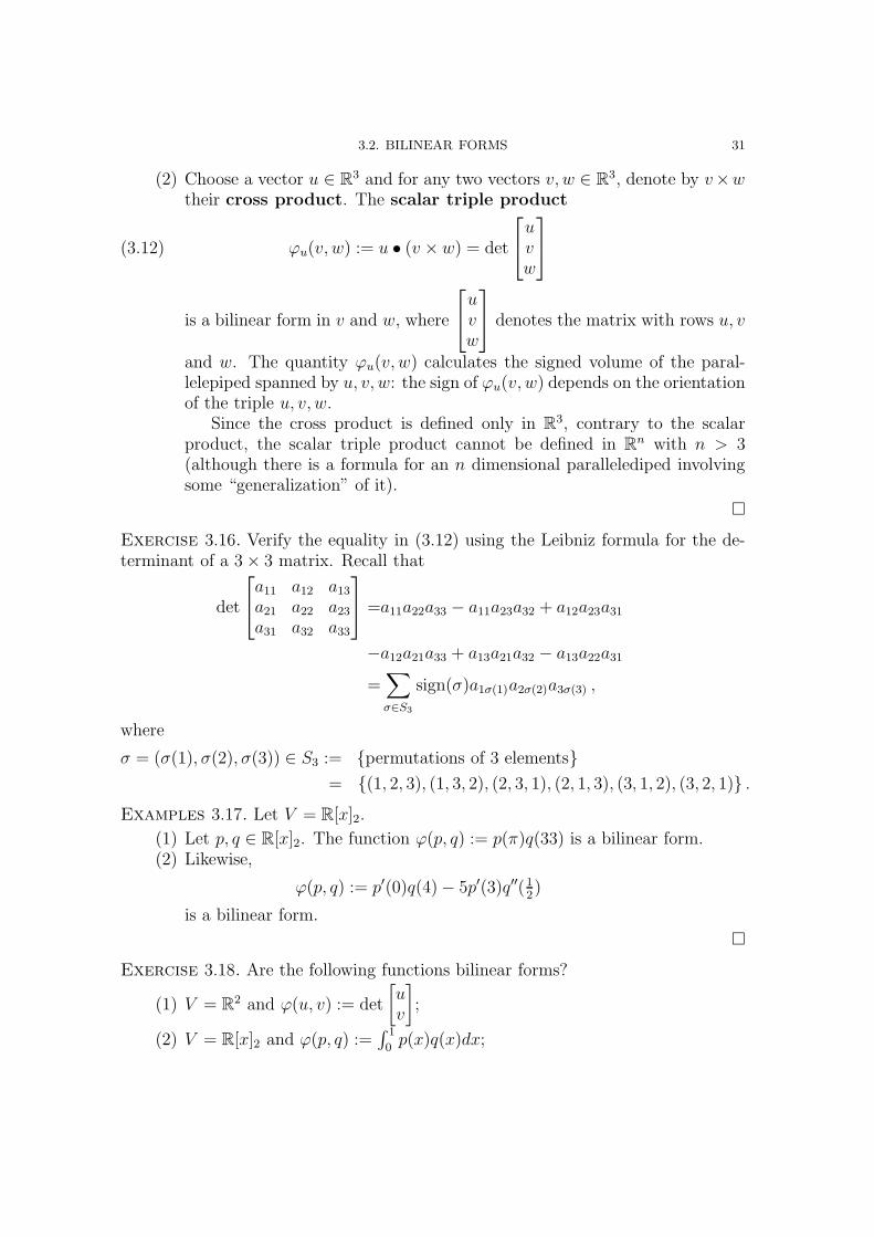
(2) Choose a vector u ∈ R3 and for any two vectors v, w ∈ R
3, denote by v×wtheir cross product. The scalar triple product
ϕu(v, w) := u • (v × w) = det
uvw
(3.12)
is a bilinear form in v and w, where
uvw
denotes the matrix with rows u, v
and w. The quantity ϕu(v, w) calculates the signed volume of the paral-lelepiped spanned by u, v, w: the sign of ϕu(v, w) depends on the orientationof the triple u, v, w.
Since the cross product is defined only in R3, contrary to the scalar
product, the scalar triple product cannot be defined in Rn with n > 3
(although there is a formula for an n dimensional parallelediped involvingsome “generalization” of it).
�
Exercise 3.16. Verify the equality in (3.12) using the Leibniz formula for the de-terminant of a 3× 3 matrix. Recall that
det
a11 a12 a13a21 a22 a23a31 a32 a33
=a11a22a33 − a11a23a32 + a12a23a31
−a12a21a33 + a13a21a32 − a13a22a31=∑
σ∈S3
sign(σ)a1σ(1)a2σ(2)a3σ(3) ,
where
σ = (σ(1), σ(2), σ(3)) ∈ S3 := {permutations of 3 elements}= {(1, 2, 3), (1, 3, 2), (2, 3, 1), (2, 1, 3), (3, 1, 2), (3, 2, 1)} .
Examples 3.17. Let V = R[x]2.
(1) Let p, q ∈ R[x]2. The function ϕ(p, q) := p(π)q(33) is a bilinear form.(2) Likewise,
ϕ(p, q) := p′(0)q(4)− 5p′(3)q′′(12)
is a bilinear form.
�
Exercise 3.18. Are the following functions bilinear forms?
(1) V = R2 and ϕ(u, v) := det
[uv
];
(2) V = R[x]2 and ϕ(p, q) :=∫ 1
0p(x)q(x)dx;
32 3. MULTILINEAR FORMS
(3) V = M2×2(R), the space of real 2 × 2 matrices, and ϕ(L,M) := L11 trM ,
where L11 it the (1,1)-entry of L and trM is the trace of M ;
(4) V = R3 and ϕ(v, w) := v × w;
(5) V = R2 and ϕ(v, w) is the area of the parallelogram spanned by v and w.
3.2.2. Tensor product of two linear forms on V . Let α, β ∈ V ∗ be twolinear forms, α, β : V → R, and define ϕ : V × V → R, by
ϕ(v, w) := α(v)β(w) .
Then ϕ is bilinear, is called the tensor product of α and β and is denoted by
ϕ = α⊗ β .Note 3.19. In general α⊗ β 6= β ⊗ α, as there could be vectors v and w such thatα(v)β(w) 6= β(v)α(w).
Example 3.20. Let V = R[x]2, let α(p) = p(2)−p′(2) and β(p) =∫ 4
3p(x)dx be two
linear forms. Then
(α⊗ β)(p, q) = (p(2)− p′(2))∫ 4
3
q(x)dx
is a bilinear form. �
Example 3.21. Let ϕ : R× R→ R be a function:
(1) ϕ(x, y) := 2x− y is a linear form in (x, y) ∈ R2;
(2) ϕ(x, y) := 2xy is bilinear, hence linear in x ∈ R and linear in y ∈ R, but itis not linear in (x, y) ∈ R
2.
�
Let
Bil(V × V,R) := {all bilinear forms ϕ : V × V → R} .
Exercise 3.22. Check that Bil(V × V,R) is a vector space with the zero elementequal to the bilinear form identically equal to zero.Hint: It is enough to check that if ϕ, ψ ∈ Bil(V × V,R), and λ, µ ∈ R, thenλϕ+ µψ ∈ Bil(V × V,R). Why? (Recall Example 2.3(4).)
Assuming Exercise 3.22, we are going to find a basis of Bil(V × V,R) and deter-mine its dimension. Let B := {b1, . . . , bn} be a basis of V and let B∗ = {β1, . . . , βn}be the dual basis of V ∗ (that is βi(bj) = δij).
Proposition 3.23. The bilinear forms β1 ⊗ βj, i, j = 1, . . . , n form a basis ofBil(V × V,R). As a consequence dimBil(V × V,R) = n2.
Notation. We denote
Bil(V × V,R) = V ∗ ⊗ V ∗
the tensor product of V ∗ and V ∗.
3.2. BILINEAR FORMS 33
Proof of Proposition 3.23. The proof will be similar to the one of Proposi-tion 3.8 for linear forms. We first check that the set of bilinear forms {β1⊗βj , i, j =1, . . . , n} span Bil(V × V,R) and than that it consists of linearly independent ele-ments.
To check that span{βi ⊗ βj, i, j = 1, . . . , n} = Bil(V × V,R), we need to checkthat if ϕ ∈ Bil(V × V,R), there exists Bij ∈ R such that
ϕ = Bijβi ⊗ βj .
Because of (3.2), we obtain
ϕ(bk, bℓ) = Bijβi(bk)β
j(bℓ) = Bijδikδ
jℓ = Bkℓ ,
for every pair (bk, bℓ) ∈ V × V . Hence we are forced to choose Bkℓ := ϕ(bk, bℓ). Nowwe have to check that with this choice of Bkℓ we have indeed
ϕ(v, w) = Bijβi(v)βj(w)
for arbitrary v = vkbk ∈ V and w = wℓbℓ ∈ V .On the one hand we have that
ϕ(v, w) = ϕ(vkbk, wℓbℓ) = vkwℓϕ(bk, bℓ) = vkwℓBkℓ ,
where the next to the last equality follows from the bilinearity of ϕ and the last onefrom the definition of Bkℓ.
On the other hand,
Bijβi(v)βj(w) = Bijβ
i(vkbk)βj(vℓbℓ)
= Bijvkβi(bk)v
ℓβj(bℓ)
= Bijvkvℓδikδ
jℓ
= Bkℓvkwℓ ,
where the second equality follows from the bilinearity of βi and the next to the lastfrom (3.2).
Now we need to check that the only linear combination of the βi⊗ βj that givesthe zero bilinear form is the trivial linear combination. Let cijβ
i ⊗ βj = 0 be alinear combination of the βi ⊗ βj . Then for all pairs of basis vectors (bk, bℓ), withk, ℓ = 1, . . . , n, we have
0 = cijβi ⊗ βj(bk, bℓ) = cijδ
ikδ
jℓ = ckℓ ,
thus showing the linear independence. �
3.2.3. Transformation of Bilinear Forms under a Change of Basis. Ifwe summarize what we have done so far, we see that once we choose a basis B :={b1, . . . , bn} of V , we automatically have a basis B∗ = {β1, . . . , βn} of V ∗ and a basis{β1 ⊗ βj, i, j = 1, . . . , n} of V ∗ ⊗ V ∗.
That is, any bilinear form ϕ : V × V → R can be represented by its components
Bij = ϕ(bi, bj)(3.13)

34 3. MULTILINEAR FORMS
and these components can be arranged in a matrix
B :=
B11 . . . B1n
......
Bn1 . . . Bnn
called the matrix of the bilinear form ϕ with respect to the chosen basis B.The natural question of course is: how does the matrix B change when we choose adifferent basis of V ?
So, let us choose a different basis B := {b1, . . . , bn} and corresponding bases
B∗ = {β1, . . . , βn} of V ∗ and {βi ⊗ βj , i, j = 1, . . . , n} of V ∗ ⊗ V ∗, with respect to
which ϕ will be represented by a matrix B, whose entries are Bij = ϕ(bi, bj).
To see the relation between B and B, due to the change of basis from B to B,we start with the matrix of the change of basis L := LBB, according to which
bj = Lijbi .(3.14)
Then
Bij = ϕ(bi, bj) = ϕ(Lki bk, L
ℓjbℓ) = Lk
iLℓjϕ(bk, bℓ) = Lk
iLℓjBkℓ ,
where the first and the last equality follow from (3.13), the second from (3.14) (after having renamed the dummy indices to avoid conflicts) and the remaining onefrom the bilinearity.
Exercise 3.24. Show that the formula of the transformation of the component ofa bilinear form in terms of the matrices of the change of coordinates is
B = tLBL ,(3.15)
where tL denotes the transpose of the matrix L.
We hence say that a bilinear form ϕ is a covariant 2-tensor or a tensor oftype (0, 2).
3.3. Multilinear forms
We saw in § 3.1.2 that linear forms are covariant 1-tensors – or tensor of type(0, 1) – and in § 3.2.3 that bilinear forms are covariant 2-tensors – or tensors of type(0, 2).
Completely analogously to what was done until now, one can define trilinearforms, that is functions T : V × V × V → R that are linear in each of the threevariables. The space of trilinear forms is denoted by V ∗ ⊗ V ∗ ⊗ V ∗, has basis{βj ⊗ βj ⊗ βk, i, j, k = 1, . . . , n} and hence dimension n3.
Since the components of a trilinear form T : V ×V ×V → R satisfy the followingtransformation with respect to a change of basis
Tijk = LℓiL
pjL
qkTℓpq ,
a trilinear form is a covariant 3-tensor or a tensor of type (0, 3).
3.4. EXAMPLES 35
In fact, there is nothing special about k = 1, 2 or 3.
Definition 3.25. A multilinear form if a function f : V × · · · × V → R fromk-copies of V into R, that is linear with respect to each variable.
A multilinear form is a covariant k-tensor or a tensor of type (0, k). Thevectors space of multilinear forms V ∗ ⊗ · · · ⊗ V ∗ has basis βi1 ⊗ βi2 × · · · ⊗ βik ,i1, . . . , ik := 1, . . . , n and hence dim(V ∗ ⊗ · · · ⊗ V ∗) = nk .
3.4. Examples
3.4.1. A Bilinear Form.
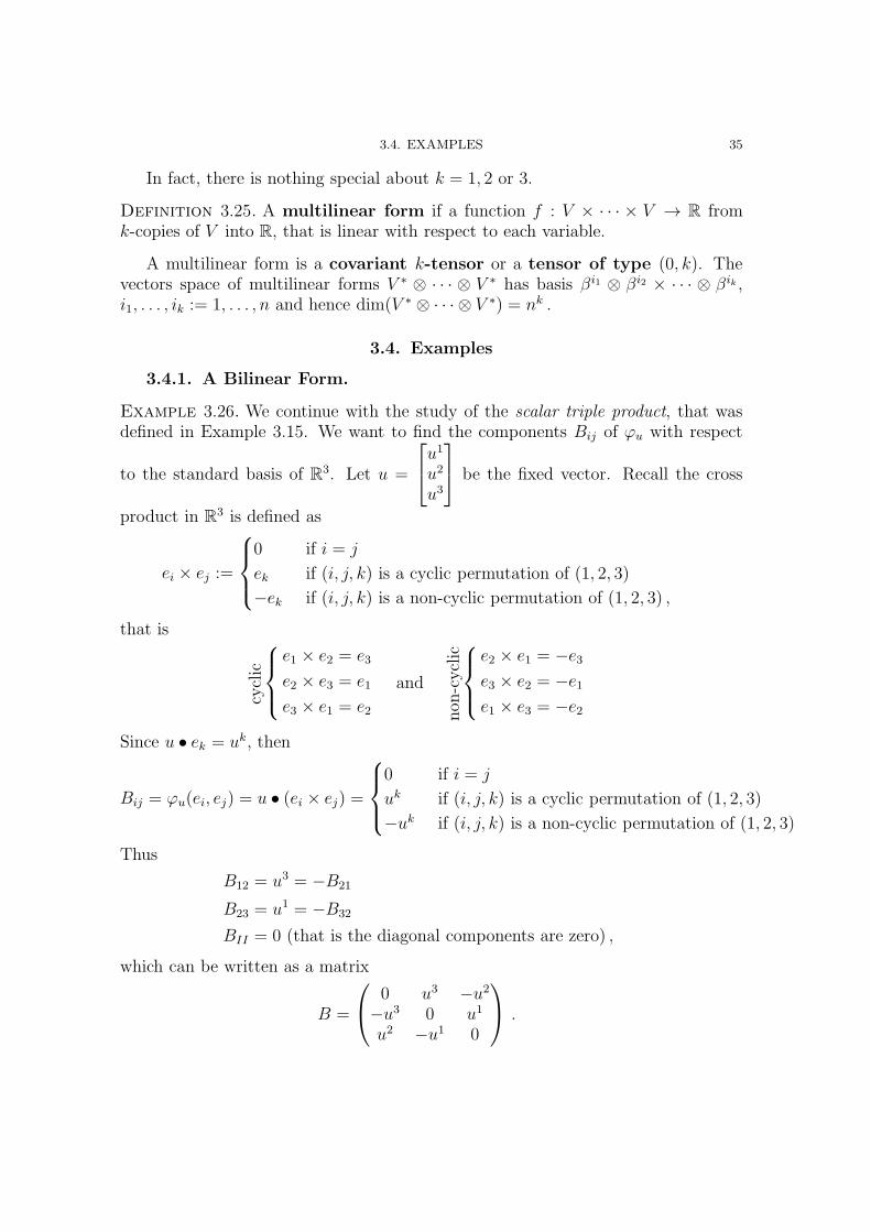
Example 3.26. We continue with the study of the scalar triple product, that wasdefined in Example 3.15. We want to find the components Bij of ϕu with respect
to the standard basis of R3. Let u =
u1
u2
u3
be the fixed vector. Recall the cross
product in R3 is defined as
ei × ej :=
0 if i = j
ek if (i, j, k) is a cyclic permutation of (1, 2, 3)
−ek if (i, j, k) is a non-cyclic permutation of (1, 2, 3) ,
that is
cyclic
e1 × e2 = e3
e2 × e3 = e1
e3 × e1 = e2
and
non
-cyclic
e2 × e1 = −e3e3 × e2 = −e1e1 × e3 = −e2
Since u • ek = uk, then
Bij = ϕu(ei, ej) = u • (ei × ej) =
0 if i = j
uk if (i, j, k) is a cyclic permutation of (1, 2, 3)
−uk if (i, j, k) is a non-cyclic permutation of (1, 2, 3)
Thus
B12 = u3 = −B21
B23 = u1 = −B32
BII = 0 (that is the diagonal components are zero) ,
which can be written as a matrix
B =
0 u3 −u2−u3 0 u1
u2 −u1 0
.
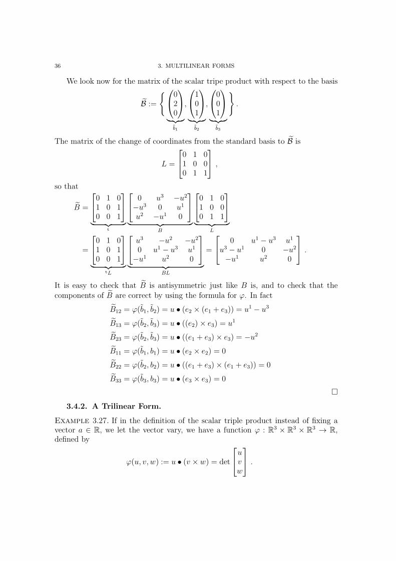
36 3. MULTILINEAR FORMS
We look now for the matrix of the scalar tripe product with respect to the basis
B :=
{020
︸ ︷︷ ︸b1
,
101
︸ ︷︷ ︸b2
,
001
︸ ︷︷ ︸b3
}.
The matrix of the change of coordinates from the standard basis to B is
L =
0 1 01 0 00 1 1
,
so that
B =
0 1 01 0 10 0 1
︸ ︷︷ ︸t
0 u3 −u2−u3 0 u1
u2 −u1 0
︸ ︷︷ ︸B
0 1 01 0 00 1 1
︸ ︷︷ ︸L
=
0 1 01 0 10 0 1
︸ ︷︷ ︸tL
u3 −u2 −u20 u1 − u3 u1
−u1 u2 0
︸ ︷︷ ︸BL
=
0 u1 − u3 u1
u3 − u1 0 −u2−u1 u2 0
.
It is easy to check that B is antisymmetric just like B is, and to check that the
components of B are correct by using the formula for ϕ. In fact
B12 = ϕ(b1, b2) = u • (e2 × (e1 + e3)) = u1 − u3
B13 = ϕ(b2, b3) = u • ((e2)× e3) = u1
B23 = ϕ(b2, b3) = u • ((e1 + e3)× e3) = −u2
B11 = ϕ(b1, b1) = u • (e2 × e2) = 0
B22 = ϕ(b2, b2) = u • ((e1 + e3)× (e1 + e3)) = 0
B33 = ϕ(b3, b3) = u • (e3 × e3) = 0
�
3.4.2. A Trilinear Form.
Example 3.27. If in the definition of the scalar triple product instead of fixing avector a ∈ R, we let the vector vary, we have a function ϕ : R3 × R
3 × R3 → R,
defined by
ϕ(u, v, w) := u • (v × w) = det
uvw
.

3.5. BASIC OPERATION ON MULTILINEAR FORMS 37
One can verify that such function is trilinear, that is linear in each of the threevariables separately.
3.5. Basic Operation on Multilinear Forms
Let T : V × · · · × V︸ ︷︷ ︸k times
→ R and U : V × · · · × V︸ ︷︷ ︸ℓ times
→ R be respectively a k-linear
and an ℓ-linear form. Then the tensor product of T and U
T ⊗ U : V × · · · × V︸ ︷︷ ︸k+ℓ times
→ R ,
defined by
T ⊗ U(v1, . . . , vk+ℓ) := T (v1, . . . , vk)U(vk+1, . . . , vk+ℓ)
is a (k + ℓ)-linear form.Likewise, one can take the tensor product of a tensor of type (0, k) and a tensor
of type (0, ℓ) to obtain a tensor of type (0, k + ℓ).

CHAPTER 4
Inner Products
4.1. Definitions and First Properties
Inner products are a special case of bilinear forms. They add an importantstructure to a vector space, as for example they allow to compute the length of avector. Moreover, they provide a canonical identification between the vector spaceV and its dual V ∗.
Definition 4.1. An inner product g : V ×V → R on a vector space V is a bilinearform on V that is
(1) symmetric, that is g(v, w) = g(w, v) for all v, w ∈ V and(2) positive definite, that is g(v, v) ≥ 0 for all v ∈ V , and g(v) = 0 if and only
if v = 0.
Exercise 4.2. Let V = R3. Determine whether the following bilinear forms are
inner products, by verifying whether they are symmetric and positive definite:
(1) the scalar or dot product ϕ(v, w) := v • w, defined as
v • w = viwi ,
where v =
v1
v2
v3
and w =
w1
w2
w3
;
(2) ϕ(v, w) := −v • w, for all v, w ∈ V ;(3) ϕ(v, w) = v • w + 2v1w2, for v, w ∈ V ;(4) ϕ(v, w) = v • 3w, for v, w ∈ V .
Exercise 4.3. Let V := R[x]2 be the vector space of polynomials of degree ≤ 2.Determine whether the following bilinear forms are inner products, by verifyingwhether they are symmetric and positive definite:
(1) ϕ(p, q) =∫ 1
0p(x)q(x)dx;
(2) ϕ(p, q) =∫ 1
0p′(x)q′(x)dx;
(3) ϕ(p, q) =∫ π
3exp(x)q(x)dx;
(4) ϕ(p, q) = p(1)q(1) + p(2)q(2);(5) ϕ(p, q) = p(1)q(1) + p(2)q(2) + p(3)q(3).
Definition 4.4. Let g : V × V → R be an inner product on V .
39
40 4. INNER PRODUCTS
(1) The norm ‖v‖ of a vector v ∈ V is defined as
‖v‖ :=√g(v, v) .
(2) A vector v ∈ V is unit vector if ‖v‖ = 1;(3) Two vectors v, w ∈ V are orthogonal (that is perpendicular or v ⊥ w),
if g(v, w) = 0;(4) Two vectors v, w ∈ V are orthonormal if they are orthogonal and ‖v‖ =‖w‖ = 1;
(5) A basis B of V is an orthonormal basis if b1, . . . , bn are pairwise orthonor-mal vectors, that is
g(bi, bj) = δij :=
{1 if i = j
0 if i 6= j ,(4.1)
for all i, j = 1 . . . , n. The condition for i = j implies that an orthonormalbasis consists of unit vectors, while the one for i 6= j implies that it consistsof pairwise orthogonal vectors.
Example 4.5. (1) Let V = R[x]2 and g the standard inner product. Thestandard basis B = {e1, . . . , en} is an orthonormal basis with respect to thestandard inner product.
(2) Let V = R[x]2 and let g(p, q) :=∫ 1
−1p(x)q(x)dx. Check that the basis
B = {p1, p2, p3} ,where
p1(x) :=1√2, p2(x) :=
√3
2x, p3(x) :=
√5
8(3x2 − 1) ,
is an orthonormal basis with respect to the inner product g.
Remark 4.6. p1, p2, p3 are the first three Legendre polynomials up toscaling.
An inner product g on a vector space V is also called a metric on V .
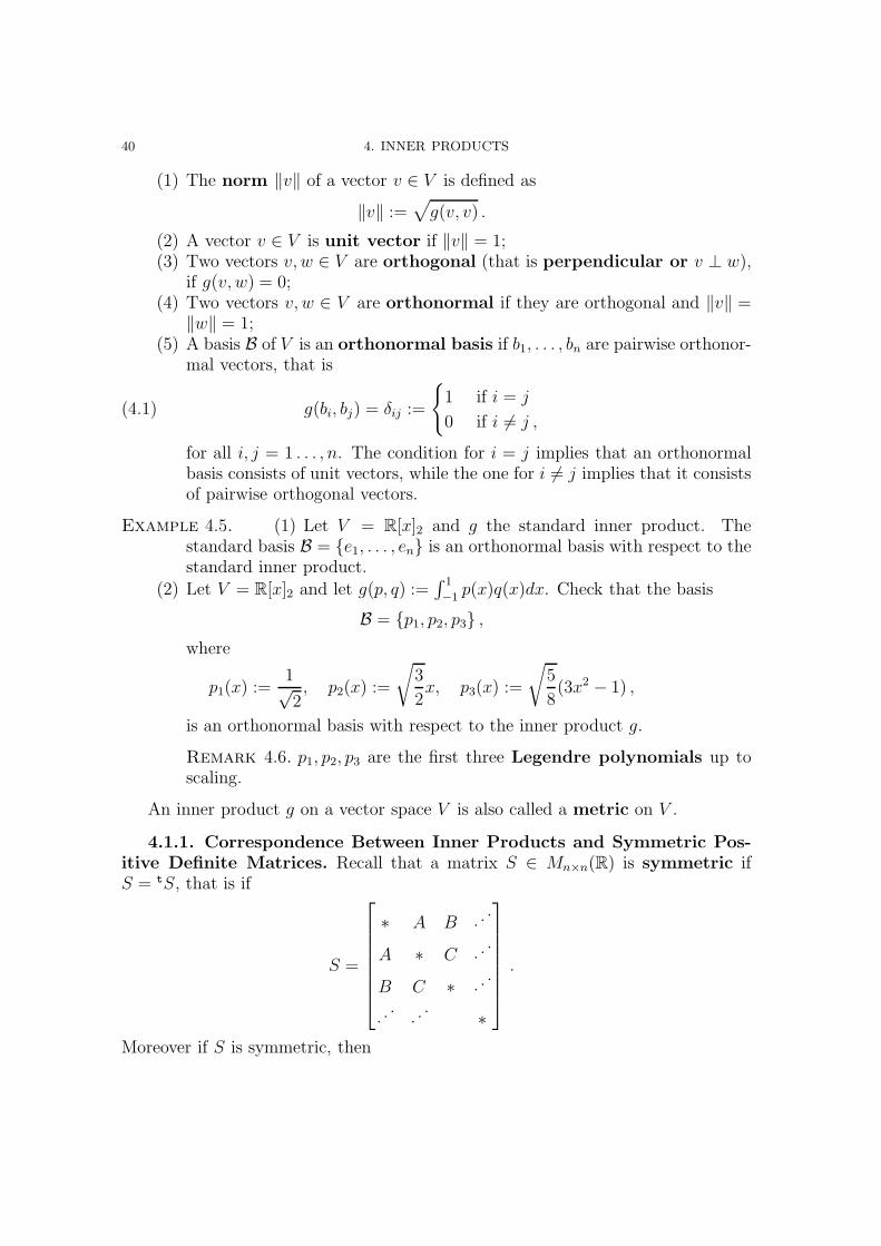
4.1.1. Correspondence Between Inner Products and Symmetric Pos-itive Definite Matrices. Recall that a matrix S ∈ Mn×n(R) is symmetric ifS = tS, that is if
S =
∗ A B ...
A ∗ C ...
B C ∗ . ..
. ... .. ∗
.
Moreover if S is symmetric, then
4.1. DEFINITIONS AND FIRST PROPERTIES 41
(1) S is positive definite if tvSv > 0 for all v ∈ Rn;
(2) S is negative definite if tvSv < 0 for all v ∈ Rn;
(3) S is positive semidefinite if tvSv ≥ 0 for all v ∈ Rn;
(4) S is positive semidefinite if tvSv ≤ 0 for all v ∈ Rn;
(5) S is indefinite if vtSv takes both positive and negative values for differentv ∈ R
n.
Definition 4.7. A quadratic form Q : Rn → R is a homogeneous quadratic
polynomial in n variables.
Any symmetric matrix S correspond to a quadratic form as follow:
S 7→ QS ,
where QS : Rn → R is defined by
QS(v) =tvSv =
[v1 . . . vn
]S
v1
...vn
︸ ︷︷ ︸matrix notation
Sij = vivjSij︸ ︷︷ ︸Einstein notation
.(4.2)
Note that Q is not linear in v.Let S be a symmetric matrix and QS be the corresponding quadratic form.
The notion of positive definiteness, etc. for S can be translated into correspondingproperties for QS, namely:
(1) Q is positive definite if Q(v) > 0 for all v ∈ V ;(2) Q is negative definite if Q(v) < 0 for all v ∈ V ;(3) Q is positive semidefinite if Q(v) ≥ 0 for all v ∈ V ;(4) Q is negative semidefinite if Q(v) ≤ 0 for all v ∈ V ;(5) Q is indefinite if Q(v) takes both positive and negative values.
To find out the type of a symmetric matrix S (or, equivalently of a quadraticform QS) it is enough to look at the eigenvalues of S, namely:
(1) S and QS are positive definite if all eigenvalues of S are positive:(2) S and QS are negative definite if all eigenvalues of S are negative;(3) S and QS are positive semidefinite if all eigenvalues of S are non-negative;(4) S and QS are negative semidefinite if all eigenvalues of S are non-positive;(5) S and QS are indefinite if S has both positive and negative eigenvalues.
The reason this makes sense is the same reason for which we need to restrict ourattention to symmetric matrices and lies in the so-called Spectral Theorem:
Theorem 4.8. [Spectral Theorem] Any symmetric matrix S has the following prop-erties:
(1) it has only real eigenvalues;(2) it is diagonalizable;
42 4. INNER PRODUCTS
(3) it admits an orthonormal eigenbasis, that is a basis {b1, . . . , bn} such thatthe bj are orthonormal and are eigenvectors of S.
4.1.1.1. From Inner Products to Symmetric Positive Definite Matrices. Let B :={b1, . . . , bn} be a basis of V . The components of g with respect to B are
gij = g(bi, bj) .(4.3)
Let G be the matrix with entries gij
G =
g11 . . . g1n...
. . ....
gn1 . . . gnn
.(4.4)
We claim that G is symmetric and positive definite. In fact:
(1) Since g is symmetric, then for 1 ≤ i, j ≤ n,
gij = g(bi, bj) = g(bj , bi) = gji ⇒ G is a symmetric matrix;
(2) Since g is positive definite, then G is positive definite as a symmetric matrix.In fact, let v = vibi, w = wjbj ∈ V be two vectors. Then, using thebilinearity of g in (1), (4.3) and with the Einstein notation, we have:
g(v, w) = g(vibi, wjbj)
(1)= viwj g(bi, bj)︸ ︷︷ ︸
gij
= viwjgij
or, in matrix notation,
g(v, w) = t[v]BG[w]B =[v1 . . . vn
]G
w1
...wn
.
4.1.1.2. From Symmetric Positive Definite Matrices to Inner Products. If S is asymmetric positive definite matrix, then the assignment
(v, w) 7→ tvSv
defines a map that is easily seen to be bilinear, symmetric and positive definite andis hence an inner product.
4.1.2. Orthonormal Basis. Suppose that there in a basis B := {b1, . . . , bn} ofV consisting of orthonormal vectors with respect to g, so that
gij = δij ,
because of Definition 4.4(5) and of (4.3). In other words the symmetric matrixcorresponding to the inner product g in the basis consisting of orthonormal vectorsis the identity matrix. Moreover
g(v, w) = viwjgij = viwjδij = viwi ,

4.1. DEFINITIONS AND FIRST PROPERTIES 43
so that, if v = w,
‖v‖2 = g(v, v) = vivi = (v1)2 + · · ·+ (vn)2 .
We deduce the following important
Fact 4.9. Any inner product g can be expressed in the standard form
g(v, w) = viwi ,
as long as [v]B =
v1
...vn
and [w]B =
w1
...wn
are the coordinates of v and w with
respect to an orthonormal basis B for g.
Example 4.10. Let g be an inner product of R3 with respect to which
B :=
{100
︸ ︷︷ ︸b1
,
110
︸ ︷︷ ︸b2
,
111
︸ ︷︷ ︸b3
}
is an orthonormal basis. We want to express g with respect to the standard basis Eof R3
E :=
{100
︸ ︷︷ ︸e1
,
010
︸ ︷︷ ︸e2
,
001
︸ ︷︷ ︸e3
}.
The matrices of the change of basis are
L := LBE =
1 1 10 1 10 0 1
and Λ = L−1 =
1 −1 00 1 −10 0 1
.
Since g is a bilinear form, we saw in (3.15) that its matrices with respect to a changeof basis are related by the formula
G = tLGL .
Since the basis B is orthonormal with respect to g, the associated matrix G is theidentity matrix, so that
G =tΛGΛ = tΛΛ
=
1 0 0−1 1 00 −1 1
1 −1 00 1 −10 0 1
=
1 −1 0−1 2 −10 −1 2
.(4.5)

44 4. INNER PRODUCTS
It follows that, with respect to the standard basis, g is given by
g(v, w) =(v1 v2 v3
)
1 −1 0−1 2 −10 −1 2
w1
w2
w3
= v1w1 − v1w2 − v2w1 + 2v2w2
−v2w3 − w3v2 + 2v3w3 .
(4.6)
�
Exercise 4.11. Verify the formula (4.6) for the inner product g in the coordinates
of the basis B by applying the matrix of the change of coordinate directly on thecoordinates vectors [v]E .
Remark 4.12. Norm and inner product of vectors depend only on the choice of g,but not on the choice of basis: different coordinate expressions yield the same result.
Example 4.13. We verify the assertion of the previous remark with the inner prod-uct in Example 4.10. Let v, w ∈ R
3 such that
[v]E =
v1
v2
v3
=
321
and [v]B =
v1
v2
v3
= L−1
v1
v2
v3
=
311
and
[w]E =
w1
w2
w3
=
123
and [w]B =
w1
w2
w3
= L−1
w1
w2
w3
=
−1−13
.
Then with respect to the basis B we have that
g(v, w) = 1 · (−1) + 1 · (−1) + 1 · 3 = 1 ,
and also with respect to the basis Eg(v, w) = 3 · 1− 3 · 2− 2 · 1 + 2 · 2 · 2− 2 · 3− 1 · 2 + 2 · 1 · 3 = 1 .
�
Exercise 4.14. Verify that ‖v‖ =√3 and ‖w‖ =
√11, when computed with respect
of both bases.
Let B := {b1, . . . , bn} be an orthonormal basis and let v = vibi be a vector in V .We want to compute the coordinates vi of v with respect of the metric g and of theelements of the basis. In fact
g(v, bj) = g(vibi, bj) = vig(bi, bj) = viδij = vj ,
that is the coordinates of a vector with respect to an orthonormal basis are the innerproduct of the vector with the basis vectors. This is particularly nice, so that wehave to make sure that we remember how to construct an orthonormal basis from agiven arbitrary basis.

4.1. DEFINITIONS AND FIRST PROPERTIES 45
Recall (Gram–Schmidt orthogonalization process). The Gram–Schmidt orthogo-nalization process is a recursive process that allows us to obtain an orthonormalbasis starting from an arbitrary one. Let B := {b1, . . . , bn} be an arbitrary basis, letg : V × V → R be an inner product and ‖ · ‖ the corresponding norm.
We start by defining
u1 :=1
‖b1‖b1 .
Next, observe that g(b2, u1)u1 is the projection of the vector b2 in the direction ofu1. It follows that
b⊥2 := b2 − g(b2, u1)u1is a vector orthogonal to u1, but not necessarily of unit norm. Hence we set
u2 :=1
‖b2‖b⊥2 .
Likewise g(b3, u1)u1 + (b3, u2)u2 is the projection of b3 on the plane generated by u1and u2, so that
b⊥3 := b3 − g(b3, u1)u1 − g(b3, u2)u2is orthogonal both to u1 and to u2. Set
u3 :=1
‖b3‖b⊥3 .
Continuing until we have exhausted all elements of the basis B, we obtain an or-thonormal basis {u1, . . . , un}.
u3
b1b1
b2 b2
b3b3 b3
u1 u1
u2 u2
Example 4.15. Let V be the subspace of R4 spanned by
b1 =
11−1−1
b2 =
2200
b3 =
1110
.
(One can check that b1, b2, b3 are linearly independent and hence form a basis of V .)We look for an orthonormal basis of V with respect to the standard inner product〈 · , · 〉. Since
‖b1‖ = (11 + 12 + (−1)2 + (−1)2)1/2 = 2⇒ u1 :=1
2b1 .

46 4. INNER PRODUCTS
Moreover
〈b2, u1〉 =1
2(1 + 1) = 2 =⇒ b⊥2 := b2 − 〈b2, u1〉u1 =
1111
,
so that
‖b2‖ = 2 and u2 =1
2
1111
.
Finally,
〈b3, u1〉 =1
2(1 + 1− 1) =
1
2and 〈b3, u2〉 =
1
2(1 + 1 + 1) =
3
2
implies that
b⊥3 := b3 − 〈b3, u1〉u1 − 〈b3, u2〉u2 =
0012−1
2
.
Since
‖b⊥3 ‖ =√2
2=⇒ u3 :=
√2
2
001−1
.
4.2. Reciprocal Basis
Let g : V × V → R be an inner product and B := {b1, . . . , bn} any basis of V .From g and B we can define another basis of V , denoted by
Bg = {b1, . . . , bn}and satisfying
g(bi, bj) = δij .(4.7)
The basis Bg is called the reciprocal basis of V with respect to g and B.Note that, strictly speaking, we are very imprecise here. In fact, while it is
certainly possible to define a set of n = dimV vectors as in (4.7), we should justifythe fact that we call it a basis. This will be done in Claim 4.18.
Remark 4.16. In general Bg 6= B and in fact, because of Definition 4.4(5),
B = Bg ⇐⇒ B is an orthonormal basis.

4.2. RECIPROCAL BASIS 47
Example 4.17. Let g be the inner product in (4.6) in Example 4.10 and let E thestandard basis of R3. We want to find the reciprocal basis Eg, that is we want tofind Eg := {b1, b2, b3} such that
g(bi, ej) = δij .
If G is the matrix of the inner product in (4.5), using the matrix notation andconsidering bj as a row vector and ei as a column vector for i, j = 1, 2, 3,
[–– tbi ––
]G
|ej|
= δij .
Letting i and j vary from 1 to 3, we obtain
–– tb1 –––– tb2 –––– tb3 ––
1 −1 0−1 2 −10 −1 2
| | |e1 e2 e3| | |
=
1 0 00 1 00 0 1
,
from which we conclude that
–– tb1 –––– tb2 –––– tb3 ––
=
| | |e1 e2 e3| | |
−1
1 −1 0−1 2 −10 −1 2
−1
=
| | |e1 e2 e3| | |
3 2 12 2 11 1 1
=
3 2 12 2 11 1 1
.
Hence
b1 =
321
, b2 =
221
, b3 =
111
.(4.8)
Observe that in order to computeG−1 we used the Gauss–Jordan elimination method
1 −1 0 1 0 0−1 2 −1 0 1 00 −1 2 0 0 1
!
1 −1 0 1 0 00 1 −1 1 1 00 −1 2 0 0 1
!
1 0 −1 2 1 00 1 −1 1 1 00 0 1 1 1 1
!
1 0 0 3 2 10 1 0 2 2 10 0 1 1 1 1
48 4. INNER PRODUCTS
4.2.1. Properties of Reciprocal Bases.
Claim 4.18. Given a vector space V with a basis B and an inner product g : V ×V →R, a reciprocal basis exists and is unique.
As we pointed out right after the definition of reciprocal basis, what this claimreally says is that there is a set of vectors {b1, . . . , bn} in V that satisfy (4.7), thatform a basis and that this basis is unique.
Proof. Let B := {b1, . . . , bn} be the given basis. Any other basis {b1, . . . , bn}is related to B by the relation
bi =M ijbj(4.9)
for some invertible matrix M . We want to show that there exists a unique matrixM such that, when (4.9) is plugged into g(bi, bj), we have
g(bi, bj) = δij .(4.10)
From (4.9) and (4.10) we obtain
δij = g(bi, bj) = g(M ikbk, bj) =M ikg(bk, bj) =M ikgkj ,
which, in matrix notation becomes
I =MG ,
where G is the matrix of g with respect to B whose entries are gij as in (4.4). SinceG is invertible because it is positive definite, thenM = G−1 exists and is unique. �
Remark 4.19. Note that in the course of the proof we have found that, since M =LBgB, then
G = (LBgB)−1 = LBBg .
We denote with gij the entries ofM = G−1. From the above discussion, it followsthat with this notation
gikgkj = δij(4.11)
as well as
bi = gijbj ,(4.12)
or(b1 . . . bn
)=(b1 . . . bn
)G−1 .(4.13)
(check for example the dimensions and the indices to understand why G−1 has tobe multiplied on the right). We can now compute g(bi, bj)
g(bi, bj)(4.12)= g(gikbk, g
jℓbℓ) = gikgjℓg(bk, bℓ)
(4.1)= gjℓδiℓ
(4.11)= gji = gij ,

4.2. RECIPROCAL BASIS 49
where we used in the second equality the bilinearity of g and in the last its symmetry.Thus, similarly to (4.1), we have
gij = g(bi, bj) .(4.14)
Given that we just proved that reciprocal basis are unique, we can talk aboutthe reciprocal basis (of a fixed vector space V associated to a basis and an innerproduct).
Claim 4.20. The reciprocal basis is contravariant.
Proof. Let B and B be two bases of V and L := LBB be the correspondingmatrix of the change of bases, with Λ = L−1. Recall that this means that
bi = Lji bj .
We have to check that if Bg = {b1, . . . , bn} is a reciprocal basis for B, then the
basis {b1, . . . , bn} defined by
bi = Λikb
k(4.15)
is a reciprocal basis for B. Then the assertion will be proven, since {b1, . . . , bn} iscontravariant by construction.
To check that {b1, . . . , bn} is the reciprocal basis, we need with check that with
the choice of bi as in (4.15), the property (4.1) of the reciprocal basis is verified,namely that
g(bi, bj) = δij .
But in fact,
g(bi, bj)(4.15)= g(Λi
kbk, Lℓ
jbℓ) = ΛikL
ℓjg(b
k, bℓ)(4.10)= Λi
kLℓjδ
kℓ = Λi
kLkj = δij ,
where the second equality comes from the bilinearity of g, the third from the property(4.7) defining reciprocal basis and the last from the fact that Λ = L−1. �
Suppose now that V is a vector space with a basis B and that Bg is the reciprocalbasis of V with respect to B and to a fixed inner product g : V × V → R. Thenthere are two ways of writing a vector v ∈ V , namely
v = vibi︸︷︷︸with respect to B
= vjbj
︸︷︷︸with respect to Bg
.
Recall that the (ordinary) coordinates of v with respect to B are contravariant
(see Example 1.2).
Claim 4.21. Vector coordinates with respect to the reciprocal basis are covariant.
50 4. INNER PRODUCTS
Proof. This will follow from the fact that the reciprocal basis is contravariantand the idea of the proof is the same as in Claim 4.20.
Namely, let B, B be two bases of V , L := LBB the matrix of the change of basis
and Λ = L−1. Let Bg and Bg be the corresponding reciprocal bases and v = vjbj a
vector with respect to Bg.It is enough to check that the numbers
vi := Ljivj
are the coordinates of v with respect to Bg, because in fact these coordinates arecovariant by definition. But in fact, using this and (4.15), we obtain
vibi = (Lj
ivj)(Λikb
k) = LjiΛ
ik︸ ︷︷ ︸
δjk
vjbk = vjb
j = v
�
Definition 4.22. The coordinates vi of a vector v ∈ V with respect to the reciprocalbasis Bg are called the covariant coordinates of v.
4.2.2. Change of basis from a basis B to its reciprocal basis Bg. We wantto look now at the direct relationship between the covariant and the contravariantcoordinates of a vector v. Recall that we can write
vibi︸︷︷︸with respect to B
= v = vjbj
︸︷︷︸with respect to Bg
.
from which we obtain
(vigij)bj = vi(gijb
j) = vibi = v = vjbj ,
and hence
vj = vigij or t[v]Bg = G[v]B , .(4.16)
Likewise, from
vibi = v = vjbj = vj(g
jibi) = (vjgji)bi
it follows that
vi = vjgji or [v]B = G−1t[v]Bg .(4.17)
Example 4.23. Let B = {e1, e2, e3} be the standard basis of R3 and let
G =
1 −1 0−1 2 −10 −1 2

4.2. RECIPROCAL BASIS 51
be the matrix of g with respect to B. In (4.8) Example 4.17 we saw that
Bg =
{b1 =
321
, b2 =
221
, b3 =
111
}
is the reciprocal basis. We find the covariant coordinates of v =
456
with respect
to Bg using (4.16), namely
[v]Bg = G[v]B =
1 −1 0−1 2 −10 −1 2
456
=(−1 0 7
).
In fact,
vibi = (−1)
321
+ 0
221
+ 7
111
=
456
.
�
Example 4.24. Let V := R[x]1 be the vector space of polynomials of degree ≤ 1(that is “linear” polynomial, or of the form a+ bx). Let g : V × V → R be definedby
g(p, q) :=
∫ 1
0
p(x)q(x)dx ,
and let B := {1, x} be a basis of V . Determine:
(1) the matrix G;(2) the matrix G−1;(3) the reciprocal basis Bg;(4) the contravariant coordinates of p(x) = 6x (that is the coordinates of p(x)
with respect to B);(5) the covariant coordinates of p(x) = 6x (that is the coordinates of p(x) with
respect to B).

52 4. INNER PRODUCTS
(1) The matrix G has entries gij = g(bi, bi), that is
g11 = g(b1, b1) =
∫ 1
0
(b1)2dx =
∫ 1
0
dx = 1
g12 = g(b1, b2) =
∫ 1
0
b1b2dx =
∫ 1
0
x =1
2
g21 = g(b2, b1) =
∫ 1
0
b2b1dx =1
2
g22 = g(b2, b2) =
∫ 1
0
(b2)2dx =
∫ 1
0
x2dx =1
3,
so that
G =
(1 1
212
13
).
(2) Since detG = 1 · 13− 1
2· 12= 1
12, then by using (2.7), we get
G−1 =
(4 −6−6 12
), .
(3) Using (4.13), we obtain that
(b1 b2
)=(1 x
)G−1 =
(1 x
)( 4 −6−6 12
)=(4− 6x −6 + 12x
),
so that Bg = {4− 6x,−6 + 12x}.
(4) p(x) = 6x = 0·1+6·x, so that p(x) has contravariant coordinates [p(x)]B =
(06
).
(5) From (4.16) it follows that if v = p(x), then(v1v2
)= G
(v1
v2
)=
(1 1
212
13
)(06
)=
(32
).
In fact, one can easily check that
v1b1 + v2b
2 = 3 · (4− 6x) + 2 · (−6 + 12x) = 6x .
4.2.3. Isomorphisms Between a Vector Space and its Dual. We sawalready in Proposition 3.8 that If V is a vector space and V ∗ is its dual, thendimV = dimV ∗. In particular this means that V and V ∗ can be identified, once wechoose a basis B of V and a basis B∗ of V ∗. In fact, the basis B∗ of V ∗ is given oncewe choose the basis B of V , as the dual basis of V ∗ with respect to B. Then thereis the following correspondence:
v ∈ V ! α ∈ V ∗ ,

4.2. RECIPROCAL BASIS 53
Table 1. Summary of covariance and contravariance of vector coordinates
B := {b1, . . . , bn} | Bg = {b1, . . . , bn}basis | reciprocal basis
they are related by g(bi, bj) = δij
v = vibi | v = vibi
contravariant | covariantcoordinates | coordinates
the matrices of g are gij = g(bi, bj) | gij = g(bi, bj)the matrices are inverse
of each other, that is gikgkj = δij
the relation between the basis |and the reciprocal basis is bi = gijb
j | bi = gijbj
the relation between covariant |coordinates and contravariant vi = gijvj | vi = gijv
j
coordinates is |
exactly when v and α have the same coordinates, respectively with respect to B andB∗, However this correspondence depends on the choice of the basis B and hencenot canonical.
If however V is endowed with an inner product, then there is a canonicalidentification of V with V ∗ (that is an identification that does not depend onthe basis B ov V ). In fact, let g : V × V → R be an inner product and let v ∈ V .Then
g(v, · ) : V −→ R
w 7−→ g(v, w)
is a linear form and hence we have the following canonical identification given bythe metric
V ←→ V ∗
v ←→ v∗ := g(v, · ) .(4.18)
Note that the isomorphism sends the zero vector to the linear form identically equalto zero, since g(v, · ) ≡ 0 if and only if v = 0, since g is positive definite.
So far, we have two bases of the vector space V , namely the basis B and thereciprocal basis Bg and we have also the dual basis of the dual vector space V ∗. Infact, under the isomorphism (4.18), the reciprocal basis of V and the dual basis ofV ∗ correspond to each other. This is easily seen because, under the isomorphism(4.18) an element of the reciprocal basis bi correspond to the linear form g(bi, · )
bi ←→ g(bi, · )

54 4. INNER PRODUCTS
and the linear form g(bi, · ) : V → R has the property that
g(bi, bj) = δij .
Hence
g(bi, · ) ≡ βi ,
and under the canonical identification between V and V ∗ the reciprocal basis of Vcorresponds to the dual basis of V ∗.
4.2.4. Geometric Interpretation. Let g : V × V → R be an inner productand B := {b1, . . . , bn} a basis of V . The orthogonal projection of a vector ∈ V ontobk is defined as
projbk v =g(v, bk)
g(bk, bk)bk .(4.19)
bk
v
projbk v
In fact, projbk v is obviously parallel to bk and the following exercises shows that thecomponent v − projbk v is orthogonal to bk.
Exercise 4.25. With projbk v defined as in , we have
v − projbk v ⊥ bk ,
where the orthogonality is meant with respect to the inner product g.
Now let v = vibi ∈ V be a vector written in terms of its covariant coordinates
(that is the coordinates with respect to the reciprocal basis). Then
g(v, bk) = g(vibi, bk) = vi g(b
i, bk)︸ ︷︷ ︸δik
= vk ,
so that (4.19) becomes
projbk v =vk
g(bk, bk)bk .
If we assume that the elements of the basis B := {b1, . . . , bn} are unit vectors,then (4.19) further simplifies to give
projbk v = vkbk .(4.20)
This equation shows the following:
Fact 4.26. The covariant coordinates of v give the orthogonal projection of v ontob1, . . . , bn.
Likewise, the following holds basically by definition:
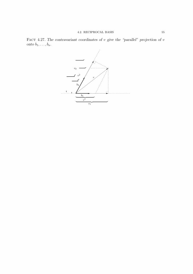
4.2. RECIPROCAL BASIS 55
Fact 4.27. The contravariant coordinates of v give the “parallel” projection of vonto b1, . . . , bn.
b1
b2
︸ ︷︷ ︸
︸ ︷︷ ︸
︸
︷︷
︸
︸
︷︷
︸
v2
v2
v1
v1
v


CHAPTER 5
Tensors
5.1. Generalities
Let V be a vector space. Up to now we saw several objects related to V , that wesaid were “tensors”. We summarize them in Table 1. So, we seem to have a goodcandidate for the definition of a tensor of type (0, q) for all q ∈ N, but we cannotsay the same for a tensor of type (p, 0) for all p ∈ N. The next discussion will leadus to that point, and in the meantime we will discuss an important point.
5.1.1. Canonical isomorphism between V and (V ∗)∗. We saw in § 4.2.3that any vector space is isomorphic to its dual, but the the isomorphism is notcanonical (that is, it depends on the choice of basis). We also saw that if there isan inner product on V , then there is a canonical isomorphism. The point of thissection is to show that, even without an inner product, there is a always a canonicalisomorphism between V and its bidual (V ∗)∗, that is the dual of its dual.
To see this, let us observe first of all that
dim V = dim(V ∗)∗ .(5.1)
If fact, for any vector space W , we saw in Proposition 3.8 that dimW = dimW ∗. Ifwe apply this equality both to W = V and to W = V ∗, we obtain
dimV = dimV ∗ and dimV ∗ = dim(V ∗)∗ ,
from which (5.1) follows immediately. From (4.2.3) we deduce immediately that Vand (V ∗)∗ are isomorphic, and we only have to see that the isomorphism is canonical.
Table 1. Covariance and Contravariance
Tensor Components Behavior under a change of basis Typevectors in V vi contravariant tensor (1,0)
linear forms V → R αj covariant tensor (0,1)
linear transformations V → V Aij mixed:
{contravariant
covarianttensor (1,1)
bilinear forms1 V × V → R Bij covariant 2-tensor (0,2)k-linear forms V × · · · × V︸ ︷︷ ︸
k
→ R Fi1i2...ik covariant k-tensor (0,k)
57

58 5. TENSORS
To this end, observe that a vector v ∈ V gives rise to a linear form on V ∗ definedby
ϕv : V∗ −→ R
α 7−→ α(v) .
Then we can define a linear map as follows:
Φ : V −→ (V ∗)∗
v 7→ ϕv{α 7→ α(v)}(5.2)
Since for any linear map T : W → W between vector spaces
dimW = dimRange(T ) + dim ker(T ) ,
it will be enough to show that ker Φ = {0}, because then
dim(V ∗)∗ = dimV = dimRange(Φ) ,
that is Φ is an isomorphism. Notice that the important fact is that we have not
chosen a basis to define the isomorphism Φ.To see that ker Φ = {0}, observe that the kernel consists of all vectors v ∈ V
such that α(v) = 0 for all α ∈ V ∗. We want to see that the only vector v ∈ V forwhich this happens is the zero vector. In fact, if 0 6= v ∈ V and B := {b1, . . . , bn}is any basis of V , then we can write v = vibi, where at least one vj 6= 0. Butthen, if B∗ = {β1, . . . , βn} is the dual basis, 0 6= vj = βj(v). Notice again that thedimension of the kernel of a linear map is invariant under a change of basis, andhence ker Φ = {0} no matter what the basis B here was.
We record this fact as follows:
Fact 5.1. Let V be a vector space and V ∗ its dual. The dual (V ∗)∗ of V ∗ iscanonically isomorphic to V .
5.1.2. Towards general tensors. Recall that
V ∗ := {α : V → R : α is a linear form} = {(0, 1)-tensors} .Applying this formula to the vector space V ∗ we obtain
(V ∗)∗ := {α : V ∗ → R : α is a linear form} .Using the isomorphism (V ∗)∗ ∼= V and the fact that coordinate vectors are con-travariant, we conclude that
{α : V ∗ → R : α is a linear form} = (V ∗)∗ = V = {(1, 0)-tensors} .So changing the vector space from V to its dual V ∗ seems to have had the effect
to transform a covariant tensor of type (0, 1) into a contravariant one of type (1, 0).We are going to apply this procedure to try to transform a covariant of type (0, 2)into a contravariant one of type (2, 0).
Recall that
{ϕ : V × V → R : bilinear } = {(0, 2)-tensors} .
5.1. GENERALITIES 59
and consider
{ϕ : V ∗ × V ∗ → R : bilinear} .
We can hence give the following definition:
Definition 5.2. A tensor of type (2, 0) is a bilinear form on V ∗, that is a bilinearfunction σ : V ∗ × V ∗ → R.
Let
Bil(V ∗ × V ∗,R) = {σ : V ∗ × V ∗ → R : σ is a bilinear form} = {(2, 0)-tensors} .
Exercise 5.3. Check that Bil(V ∗ × V ∗,R) is a vector space, that is that if σ, τ ∈Bil(V ∗ × V ∗,R) and λ, µ ∈ R, then λσ + µτ ∈ Bil(V ∗ × V ∗,R).
5.1.3. Tensor product of (1, 0)-tensors on V ∗. If v, w ∈ V are two vectors(that is two (1, 0)-tensors), we define
σv,w : V ∗ × V ∗ → R
by
σv,w(α, β) := α(v)β(w) .
Since α and β are two linear forms, then σ
σv,w =: v ⊗ w
is bilinear and called the tensor product of v and w. Hence σ is a (2, 0)-tensor.
Note 5.4. In general
v ⊗ w 6= w ⊗ v ,
as there can be linear forms α, β such that α(v)β(w) 6= α(w)β(v).
Similar to what we saw in § 3.2.2, we can define a basis for the space of (2, 0)-tensors by considering the (2, 0)-tensors defined by bi ⊗ bj , where B := {b1, . . . , bn}is a basis of V .
Proposition 5.5. The elements bj ⊗ bj , i, j = 1, . . . , n form a basis of Bil(V ∗ ×V ∗,R). Thus dimBil(V ∗ × V ∗,R) = n2.
We will not prove the proposition here, as the proof is be completely analogousto the one of Proposition 3.23.
Notation. We write
Bil(V ∗ × V ∗,R) = V ⊗ V .
60 5. TENSORS
5.1.4. Components of a (2, 0)-tensor and their contravariance. Let σ :V ∗ × V ∗ → R be a bilinear form on V ∗, that is a (2, 0)-tensor, as we just saw. Wewant to verify that it behaves as we expect with respect to a change of basis. Afterchoosing a basis B := {b1, . . . , bn} of V , we have the dual basis B∗ = {β1, . . . , βn}of V ∗ and the basis {bi ⊗ bj : i, j = 1, . . . , n} of the space of (2, 0)-tensors.
The (2, 0)-tensor σ is represented by its components
Sij = σ(βi, βj) ,
that is
σ = Sijbj ⊗ bj ,and the components Sij can be arranged into a matrix
S =
S11 . . . S1n
.... . .
...Sn1 . . . Snn
called the matrix of the (2, 0)-tensor with respect to the chosen basis of V .We look now at how the components of a (2, 0)-tensor change with a change
of basis. Let B := {b1, . . . , bn} and B := {b1, . . . , bn} be two basis of V and let
B∗ := {β1, . . . , βn} and B∗ := {β1, . . . , βn} be the corresponding dual basis of V ∗.Let σ : V ∗ × V ∗ → R be a (2, 0)-tensor with components
Sij = σ(βi, βj) and Sij = σ(βi, βj)
with respect to B∗ and B∗ respectively. Let L := LBB be the matrix of the change
of basis from B to B, and let Λ = L−1. Then, as seen in (1.2) and (3.11) we havethat
bj = Lijbi and βi = Λi
jβj .
It follows that
Sij = σ(βi, βj) = σ(Λikβ
k,Λjℓβ
ℓ) = ΛikΛ
jℓσ(β
k, βℓ) = ΛikΛ
jℓS
kℓ ,
where the first and the last equality follow from the definition of Sij and of Skℓ
respectively, the second from the change of bases and the third from the bilinearityof σ. We conclude that
Sij = ΛikΛ
jℓS
kl .(5.3)
Hence σ is a contravariant 2-tensor..
Exercise 5.6. Verify that in terms of matrices (5.3) translates into
S = tΛSΛ .
(Compare with (3.15).)
5.3. TENSOR PRODUCT 61
5.2. Tensors of type (p, q)
Definition 5.7. A tensor of type (p, q) or (p, q)-tensor is a multilinear form
T : V ∗ × . . . V ∗︸ ︷︷ ︸
p
×V × · · · × V︸ ︷︷ ︸q
−→ R .
Let T be a (p, q)-tensor, B := {b1, . . . , bn} a basis of V and B∗ = {β1, . . . , βn} thecorresponding dual basis of V ∗. The components of T with respect to these basesare
Ti1,...,ipj1,...,jq
= T (βi1, . . . , βip, bj1 , . . . , bjq) .
If moreover B := {b1, . . . , bn} is another basis, B∗ = {β1, . . . , βn} is the corespondingdual basis of V ∗ and L := LBB is the matrix of the change of basis with inverseΛ := L−1, then the components of T with respect to these new bases are
Ti1,...,ipj1,...,jq
= Λi1k1. . .Λ
ipkpLℓ1j1. . . L
ℓqjqT
k1,...,lpℓ1,...,ℓq
.
5.3. Tensor product
We saw already in § 3.2.2 and § 3.5 the tensor product of two multilinear forms.Since multilinear forms are covariant tensors, we said that this corresponds to thetensor product of two covariant tensors. More generally, we can define the tensorproduct of any two tensors as follows:
Definition 5.8. Let
T : V ∗ × . . . V ∗︸ ︷︷ ︸
p
×V × · · · × V︸ ︷︷ ︸q
−→ R
be a (p, q)-tensor and
U : V ∗ × . . . V ∗︸ ︷︷ ︸
k
×V × · · · × V︸ ︷︷ ︸ℓ
−→ R
a (k, ℓ) tensor. The tensor product T ⊗ U of T and U is a (p+ k, q + ℓ)-tensor
T ⊗ U : V ∗ × . . . V ∗︸ ︷︷ ︸
p+k
×V × · · · × V︸ ︷︷ ︸q+ℓ
−→ R
defined by
(T ⊗ U)(α1, . . . , αp+k, v1, . . . , vq+ℓ) :=
T (α1, . . . , αp, v1, . . . , vq)U(αp+1, . . . , αp+k, vq+1, . . . , vq+ℓ) .
Note that both T ⊗U and U ⊗ T are tensors of the same type (p+ k, q+ ℓ), butin general
T ⊗ U 6= U ⊗ T .
62 5. TENSORS
The set of all tensors of type (p, q) on a vector space V is denoted by
T pq (V ) := {all (p, q)-tensors on V } .
Analogously to how we proceeded in the case of (0, 2)-tensors, we compute thedimension of T p
q (V ). If B := {b1, . . . , bn} is a basis of V and B∗ := {β1, . . . , βn} isthe corresponding dual basis of V ∗. Just like we saw in Proposition 5.5 in the caseof (0, 2)-tensors, a basis of T p
q (V ) is
{bi1 ⊗ bi2 ⊗ · · · ⊗ bip ⊗ βj1 ⊗ βj2 ⊗ · · · ⊗ βjq : 1 ≤ i1, . . . , ip ≤ n, 1 ≤ j1, . . . , jq ≤ n} .Since there are n× · · · × n︸ ︷︷ ︸
p
×n× · · · × n︸ ︷︷ ︸q
= np+q elements in this basis (correspond-
ing to the possible choices of bik and βjℓ), we deduce that
dim T pq (V ) = np+q .
We now define the tensor product of two vector spaces:
Definition 5.9. Let V andW be two finite dimensional vector spaces, with dim V =n and dimW = m. Choose {b1, . . . , bn} a basis of V and {a1, . . . , am} a basis of W .Then the tensor product V ⊗W of V and W is an (n ·m)-dimensional vectorspace with basis
{bi ⊗ aj : 1 ≤ i ≤ n, 1 ≤ j ≤ m} .We remark that there is no reason to restrict oneself to the tensor product of
only two factors. One can equally define the tensor product V1⊗· · ·⊗Vk, and obtaina vector space of dimension dimV1 × · · · × dimVk.
There is hence an identification
T pq (V ) ∼= V ⊗ · · · ⊗ V︸ ︷︷ ︸
p
⊗V ∗ ⊗ · · · ⊗ V ∗︸ ︷︷ ︸
q
,
that follows from the fact that both spaces have the same basis. The followingproposition gives other useful identifications.
Proposition 5.10. Let V and W be two finite dimensional vector spaces, withdimV = n and dimW = m and let us denote by
Lin(V,W ∗) := {linear maps V →W ∗} .Then
Bil(V ×W,R) ∼= Lin(V,W ∗)∼= Lin(W,V ∗)∼= V ∗ ⊗W ∗
∼= (V ⊗W )∗
∼= Lin(V ⊗W,R) .

5.3. TENSOR PRODUCT 63
Proof. Here is the idea behind this chain of identifications. Let f ∈ Bil(V ×W,R), that is a bilinear function f : V ×W → R. This means that f takes twovectors, v ∈ V and w ∈ W , as input and gives back a real number f(v, w) ∈ R. Ifon the other hand we only feed f one vector v ∈ V , then there is a remaining spotwaiting for a vector w ∈ W to produce a real number. Since f is linear on V andon W , the map f(v, · ) : W → R is a linear form, so f(v, · ) ∈ W ∗. In other words,we can view f ∈ Lin(V,W ∗). It follows that there is a linear map
Bil(V ×W,R) −→ Lin(V,W ∗)
f 7−→ Tf ,
where
Tf (v)(w) := f(v, w) .
Conversely, any T ∈ Lin(V,W ∗) can be identified with a bilinear map fT ∈ Bil(V ×W,R) defined by
fT (v, w) := T (v)(w) .
Since fTf= f and TfT = T , we have proven the first identification in the proposition.
Analogously, if the input is only a vector w ∈ W , then f( · , w) : V → R is a linearmap and hence f ∈ Bil(V ×W,R) defines a linear map Tf ∈ Lin(W,V ∗). The samereasoning as in the previous paragraph, shows that Bil(V ×W,R) ∼= Lin(W,V ∗).
To proceed with the identifications, observe that, because of our definition ofV ∗ ⊗W ∗, we have
Bil(V ×W,R) ∼= V ∗ ⊗W ∗ ,
since these spaces both have basis2
{βi ⊗ αj : 1 ≤ i ≤ n, 1 ≤ j ≤ m} ,where {b1, . . . , bn} is a basis of V with corresponding dual basis {β1, . . . , βn} of V ∗,and {a1, . . . , an} is a basis of W with corresponding dual basis {α1, . . . , αn} of W ∗.
Finally, an element Dijβi ⊗ αj ∈ V ∗ ⊗ W ∗ may be viewed as a linear map
V ⊗W → R, that is as an element of (V ⊗W )∗ by
V ⊗W −→ R
Ckℓbk ⊗ aℓ 7−→ DijCkℓ βi(bk)︸ ︷︷ ︸
δik
αj(aℓ)︸ ︷︷ ︸δjℓ
= DijCkℓ .
�
Because of the identification Bil(V ×W,R) ∼= Lin(V ⊗W,R), sometimes one saysthat “the tensor product linearizes what was bilinear or multilinear”.
2There is a way of defining the tensor product of vector spaces without involving bases, butwe will not do it here.


CHAPTER 6
Applications
6.1. Inertia tensor
6.1.1. Moment of inertia with respect to the axis determined by theangular velocity. Let M be a rigid body fixed at a point O. The motion of thisrigid body at time t is by rotation by an angle θ with angular velocity ω about someaxis through O. The angular velocity has magnitude | · | or ‖ · ‖
|ω| =∣∣∣∣dθ
dt
∣∣∣∣ ,
direction given by the axis of rotation and orientation by the right-hand rule. Theposition vector of a point P in the body M relative to the origin O is
x =−→OP
while the linear velocity of a point P is
v = ω × x .
The linear velocity v has magnitude
|v| = |ω|︸︷︷︸|dθdt ||x| sinα︸ ︷︷ ︸
r
and direction tangent at P to the circle of radius r perpendicular to the axis ofrotation.
65
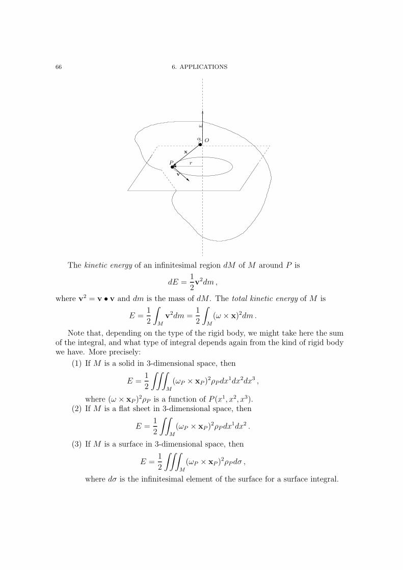
66 6. APPLICATIONS
..α
r
O
P
x
v
ω
The kinetic energy of an infinitesimal region dM of M around P is
dE =1
2v2dm ,
where v2 = v • v and dm is the mass of dM . The total kinetic energy of M is
E =1
2
∫
M
v2dm =1
2
∫
M
(ω × x)2dm .
Note that, depending on the type of the rigid body, we might take here the sumof the integral, and what type of integral depends again from the kind of rigid bodywe have. More precisely:
(1) If M is a solid in 3-dimensional space, then
E =1
2
∫∫∫
M
(ωP × xP )2ρPdx
1dx2dx3 ,
where (ω × xP )2ρP is a function of P (x1, x2, x3).
(2) If M is a flat sheet in 3-dimensional space, then
E =1
2
∫∫
M
(ωP × xP )2ρPdx
1dx2 .
(3) If M is a surface in 3-dimensional space, then
E =1
2
∫∫∫
M
(ωP × xP )2ρPdσ ,
where dσ is the infinitesimal element of the surface for a surface integral.

6.1. INERTIA TENSOR 67
(4) If M is a wire in 3-dimensional space, then
E =1
2
∫
M
(ωP × xP )2ρPds ,
where ds is the infinitesimal element of length for a line integral.(5) If M is a finite set of point masses with rigid relative positions, then
E =1
2
N∑
i=1
(ωP × xi)2mi .
In any case we need to work out the quantity
(ω × x)2
for vectors ω and xi in 3-dimensional space.To this purpose we use the Lagrange identity1, according to which
(a× b) · (c× d) = det
[a · c a · db · c b · d
].(6.1)
Applying (6.1) with a = c = ω and b = d = x, we obtain
(ω × x)2 = (ω × x) · (ω × x) = det
[ω · ω ω · xx · ω x · x
]= ω2x2 − (ω · x)2 .
Let now B = {e1, e2, e3} be an orthonormal2 basis of R, so that
ω = ωiei and x = xiei .
Then
ω2 = ω · ω = δijωiωj = ω1ω1 + ω2ω2 + ω3ω3
x2 = x · x = δkℓxkxℓ = x1x1 + x2x2 + x3x3
ω · x = δikωixk
so that
(ω × x)2 = ω2x2 − (ω · x)2
= (δijωiωj)(δkℓx
kxℓ)− (δikωixk)(δjlω
jxℓ)
= (δijδkℓ − δikδjℓ)ωiωjxkxℓ .
Therefore the total kinetic energy is
E =1
2(δijδkℓ − δikδjℓ)ωiωj
∫
M
xkxℓdm
and it depends only on ω1, ω2, ω3 (since we have integrated over the x1, x2, x3).
1The Lagrange identity can easily be proven in coordinates.2We could use any basis of R3. Then, instead of the δij , the formula would have involved
the metric tensor gij . However computations with orthonormal bases are simpler. In additionin this case we will see that the metric tensor is symmetric, and hence it admits an orthonormaleigenbasis.

68 6. APPLICATIONS
Definition 6.1. The inertia tensor is the tensor whose components with respectto an orthonormal basis B are
Iij = (δijδkℓ − δikδjℓ)∫
M
xkxℓdm .
Then the kinetic energy of the rotating rigid body is
E =1
2Iijω
iωj
︸ ︷︷ ︸Einsteinnotation
=1
2ω · Iω︸ ︷︷ ︸matrixnotation
.
One can check that
I11 =
∫
M
(x2x2 + x3x3)dm
I22 =
∫
M
(x1x1 + x3x3)dm
I33 =
∫
M
(x1x1 + x2x2)dm
I23 = I32 = −∫
M
x2x3dm
I31 = I13 = −∫
M
x1x3dm
I12 = I21 = −∫
M
x1x2dm ,
so that with respect to the basis B, the metric tensor is represented by the symmetricmatrix
I =
I11 I12 I13I21 I22 I23I31 I32 I33
.
We check only the formula for I11. In fact,
I11 = (δ11δkℓ︸ ︷︷ ︸=0
unlessk=ℓ
− δ1kδ1ℓ︸ ︷︷ ︸=0
unlessk=ℓ=1
)
∫
M
xkxℓdm
If k = ℓ = 1, then δ11δ11−δ11δ11 = 0, so that the non-vanishing terms have k = ℓ 6= 1.So I11, I22, I33 are the moments of inertia of the rigid body M with respect to
the axes Ox1, Ox2, Ox3 respectively; I12, I23, I31 are the polar moments of inertiaor the products of inertia of the rigid body M .
Example 6.2. Find the inertia tensor of a homogeneous rectangular plate with sidesa and b and total mass m, assuming that the center of rotation O coincides with

6.1. INERTIA TENSOR 69
the center of inertia. We choose an orthonormal basis with e1 aligned with the sideof length a, e2 aligned with the side of length b and e3 perpendicular to the plate.
.e1
e2
a
b
Since the plate is assumed to be homogeneous, it has a constant mass density
equal to
ρ =total mass
area=m
ab.
Denote by x, y and z the coordinates. Then
I11︸︷︷︸Ixx
=
∫ a2
− a2
∫ b2
− b2
(y2 + z2︸︷︷︸=0
) ρ︸︷︷︸mab
dydx
=m
aba
∫ b2
− b2
y2dy
=m
b
[y3
3
] b2
− b2
=m
12b2 .
Similarly
I22︸︷︷︸Iyy
=m
12a2 ,
and
I33︸︷︷︸Izz
=
∫ a2
− a2
∫ b2
− b2
(x2 + y2)ρ dydx =m
12(a2 + b2) ,
which turns out to be just the sum of I11 and I22.
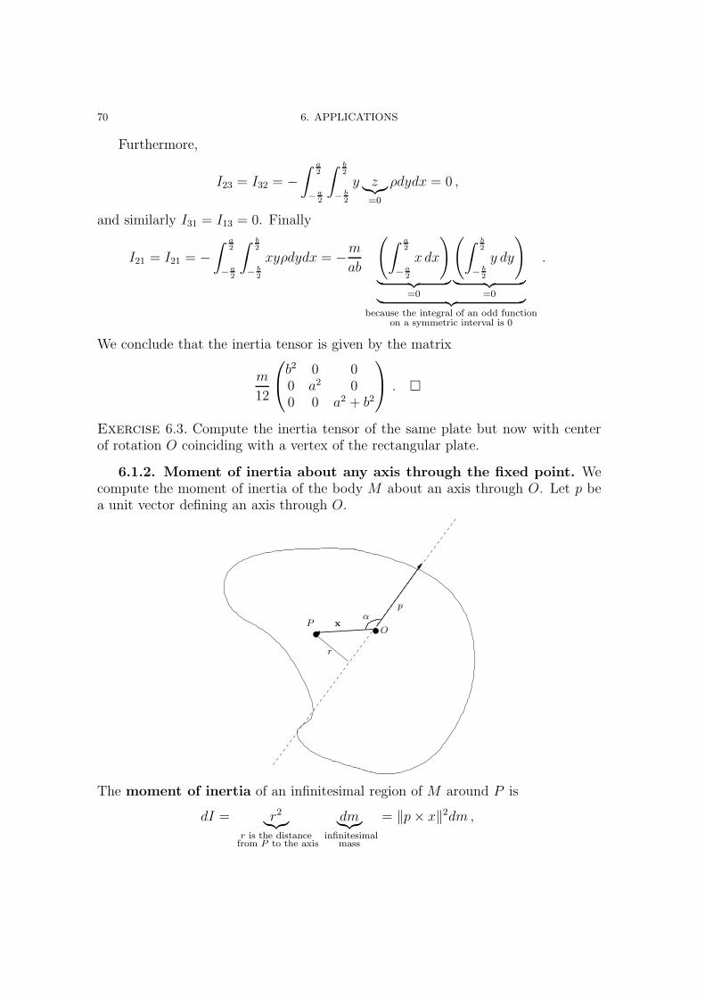
70 6. APPLICATIONS
Furthermore,
I23 = I32 = −∫ a
2
− a2
∫ b2
− b2
y z︸︷︷︸=0
ρdydx = 0 ,
and similarly I31 = I13 = 0. Finally
I21 = I21 = −∫ a
2
− a2
∫ b2
− b2
xyρdydx = −mab
(∫ a2
− a2
x dx
)
︸ ︷︷ ︸=0
(∫ b2
− b2
y dy
)
︸ ︷︷ ︸=0︸ ︷︷ ︸
because the integral of an odd functionon a symmetric interval is 0
.
We conclude that the inertia tensor is given by the matrix
m
12
b2 0 00 a2 00 0 a2 + b2
. �
Exercise 6.3. Compute the inertia tensor of the same plate but now with centerof rotation O coinciding with a vertex of the rectangular plate.
6.1.2. Moment of inertia about any axis through the fixed point. Wecompute the moment of inertia of the body M about an axis through O. Let p bea unit vector defining an axis through O.
. .αr
OP x
p
The moment of inertia of an infinitesimal region of M around P is
dI = r2︸︷︷︸r is the distancefrom P to the axis
dm︸︷︷︸infinitesimal
mass
= ‖p× x‖2dm ,

6.1. INERTIA TENSOR 71
where the last equality follows from the fact that ‖p× x‖ = ‖p‖ ‖x‖ sinα = r, sincep is a unit vector. Hence the total moment of inertia of M with respect to theaxis given by p is
I =
∫
M
‖p× x‖2dm ≥ 0 .
(This is very similar to the total kinetic energy E: just replace ω by p and omit thefactor 1
2.) By the earlier computations, we conclude that
I = Iijpipj ,
where Iij is the inertia tensor. This formula shows that the total moment of inertia
of the rigid body M with respect to an arbitrary axis passing through the point O is
determined only by the inertia tensor of the rigid body.
Example 6.4. For the rectangular plate in Example 6.2, compute the moment ofinertia with respect to the diagonal of the plate.
.O
a
b
Choose p = 1√a2+b2
(ae1 + be2) (the other possibility is the negative of this vector).
So
p1 =a√
a2 + b2, p2 =
b√a2 + b2
p3 = 0 .
The moment of inertia is
I =Iijpipj
=(
a√a2+b2
b√a2+b2
0)
m12b2 0 00 m
12a2 0
0 0 m12(a2 + b2)
a√a2+b2b√
a2+b2
0
=m
6
a2b2
a2 + b2. �

72 6. APPLICATIONS
6.1.3. Moment of inertia with respect to an eigenbasis of the inertiatensor. Observe that the inertia tensor is symmetric and recall the spectral the-orem for symmetric matrices that we saw in Theorem 4.8. Let (e1, e2, e3) be anorthonormal basis for the inertia tensor of a rigid body M . Let I1, I2, I3 be thecorresponding eigenvalues of the inertia tensor. The matrix representing the inertiatensor with respect to this eigenbasis is
I1 0 00 I2 00 0 I3
.
The axes of the eigenvectors e1, e2, e3 are called the principal axes of inertiaof the rigid body M . The eigenvalues Ii are called the principal moments ofinertia.
The principal moments of inertia are the moments if inertia with respect to theprincipal axes of inertia, hence they are non-negative
I1, , I2, , I3 ≥ 0 .
A rigid body is called
(1) an asymmetric top if I1 6= I2 6= I3 6= I1;(2) a symmetric top if I1 = I2 6= I3: any axis passing through the plane
determined by e1 and e2 is a principal axis of inertia;(3) a spherical top if I1 = I2 = I3: any axis passing through O is a principal
axis of inertia.
With respect to the eigenbasis {e1, e2, e3} the kinetic energy is
E =1
2(I1(ω
1)2 + I2(ω2)2 + I3(ω
3)2) ,
where ω = ωiei, with ωi the components of the angular velocity with respect to the
basis {e1, e2, e3}.The surface determined by the equation (with respect to the coordinates x, y, z)
I1x2 + I2y
2 + I3z2 = 1
is called the ellipsoid of inertia. The symmetry axes of the ellipsoid coincide withthe principal axes of inertia. Note that for a spherical top, the ellipsoid of inertia isactually a sphere.
The ellipsoid of inertia gives the moment of inertia with respect to any axisas follows: Consider an axis given by the unit factor p and let q be a vector ofintersection of the axis with the ellipsoid of inertia.
q = cp
where c is the (signed) distance to O of the intersection of the axis with the ellipsoidof inertia.

6.1. INERTIA TENSOR 73
O
qp
axis
The moment of inertia with respect to this axis if
I = Iijpipj =
1
c2Iijq
iqj =1
c2,
where the last equality follows from the fact that, since q is on the ellipsoid, thenIijq
iqj = 1.
6.1.4. Angular momentum. Let M be a body rotating with angular velocity
ω about an axis through the point O. Let x =−→OP be the position vector of a point
P and v = ω × x the linear velocity of P .
..α O
P
x
v
ω

74 6. APPLICATIONS
Then the angular momentum of an infinitesimal region of M around P is
dL = (x× v)dm ,
so that the total angular momentum of M is
L =
∫
M
(x× (ω × x))dm .
We need to work out x× (ω×x) for vectors x and ω in three dimensional space.It is easy to prove, using coordinates3, the equality
x× (ω × x) = ω(x • x)− x(ω • x) .(6.2)
Let B = {e1, e2, e3} be an orthonormal basis of R3. Then, replacing the followingequalities
ω = ωiei = δijωjei(6.3)
x = xiei = δikxkei(6.4)
x • x = δkℓxkxℓ(6.5)
ω • x = δjℓωjxℓ(6.6)
into (6.2), we obtain
x× (ω × x) = δijωjei︸ ︷︷ ︸
(6.3)
(δkℓxkxℓ︸ ︷︷ ︸
(6.5)
)− δikxkei︸ ︷︷ ︸(6.4)
(δjℓωjxℓ︸ ︷︷ ︸
(6.6)
) = (δijδkℓ − δikδjℓ)ωjxkxℓei .
Therefore the total angular momentum is
L = Liei ,
where the components Li are
Li = (δijδkℓ − δikδjℓ)ωj
∫
M
xkxℓdm .
Since we restrict to orthonormal bases, we have always
δij = δij = δij =
{1 if i = j
0 if i 6= j.
Hence the above expression for Li can be written in terms of the inertia tensor Iijas
Li = Iijωj .
3Consider only the case in which x is a basis vector and use the linearity in ω.
6.2. STRESS TENSOR (SPANNUNG) 75
Example 6.5. Suppose the rectangular plate in the previous examples is rotatingabout an axis through O with angular velocity
ω = e1 + 2e2 + 3e3 , or
ω1
ω2
ω3
=
123
.
Compute its angular momentum.The inertia tensor is given by the matrix Iij
m12b2 0 00 m
12a2 0
0 0 m12(a2 + b2)
.
The total angular momentum has components given by
m12b2 0 00 m
12a2 0
0 0 m12(a2 + b2)
123
=
m12b2
m6a2
m4(a2 + b2)
=
L1
L2
L3
,
so that
L =m
12b2e1 +
m
6a2e2 +
m
4(a2 + b2)e3 .
6.2. Stress tensor (Spannung)
It was the concept of stress in mechanics that originally led to the invention oftensors
tenseur
&&▲▲▲
▲▲▲▲
▲▲▲
stress
99rrrrrrrrrr
%%▲▲▲
▲▲▲▲
▲▲▲
tensor
tension
88rrrrrrrrrr
Let us consider a rigid body M acted upon by external forces but in static
equilibrium, and let us consider an infinitesimal region dM around a point P . Thereare two types of external forces:
(1) The body forces, that is forces whose magnitude is proportional to thevolume/mass of the region. For instance, gravity, attractive force or thecentrifugal force.
(2) The surface forces, that is forces exerted on the surface of the element bythe material surrounding it. They are forces whose magnitude is propor-tional to the area of the region in consideration.

76 6. APPLICATIONS
The surface force per unit area is called the stress. We will concentrate on homo-geneous stress, that is stress that does not depend on the location of the elementin the body, but depends only on the orientation of the surface/plane. Moreover,we assume that the body in consideration is in static equilibrium.
Choose an orthonormal basis {e1, e2, e3} and the plane π through P parallel tothe e2e3 coordinate plane. The normal to the plane is the vector e1. Let ∆A1 bethe area of the slice of the infinitesimal region around P cut by the plane and let∆F be the force acting on that slice. We write ∆F in terms of its components
∆F = ∆F 1e1 +∆F 2ee +∆F 3e3
and, since we defined the stress to be the surface force per unit area, we define, forj = 1, 2, 3,
σ1j := lim∆A1→0
∆F j
∆A1.
Similarly we can consider planes parallel to the other coordinate planes
e1 e2
e3
P
PP
π1
π2
π3
and define
σij := lim∆Ai→0
∆F j
∆Ai.
It turns out that the resulting nine numbers σij form a contravariant 2-tensor calledthe stress tensor. To see this, we compute the stress tensor across other slicesthrough P , that is other planes with other normal vectors. Let Π be a plane passingthrough P , n the unit vector through P perpendicular to the plane π, ∆s = π∩dMthe area of a small element of the plane Π containing P and ∆F the force acting onthat element.
Π∆s
n
P
Claim 6.6. The stress at P across the surface perpendicular to n is
σ(n)def= lim
∆s→0
∆F
∆s= σij(n • ei)ej .

6.2. STRESS TENSOR (SPANNUNG) 77
It follows from the claim that the stress σ is a vector valued function that dependslinearly on the normal n to the surface element, and we will see in § 6.2.2 that thematrix σij of this linear vector valued function forms a second-order tensor.
Proof. Consider the tetrahedron OA1A2A3 formed by the triangular slice onthe plane Π having area ∆s and three triangles on planes parallel to the coordinateplanes
e1
e2
e3
O
n
α1
α2
α3
Consider all forces acting on this tetrahedron as a volume element of the rigid body.There can be two types of forces:
(1) Body forces= f •∆v, where f is the force per unit of volume and ∆v is thevolume of the tetrahedron. We actually do not know these forces, but wewill see later that this is not relevant.
(2) Surface forces, that is the sum of the forces on each of the four sides of thetetrahedron.
We want to assess each of the four surface contributions due to the surface forces.If ∆s is the area of the slice on the plane Π, the contribution of that slice is
σ(n)∆s .
If ∆s1 is the area of the slice on the plane with normal −e1, the contribution of thatslice is
−σ1jej∆s1 ,
and similarly the contributions of the other two slices are
−σ2jej∆s2 and − σ3jej∆s3 .
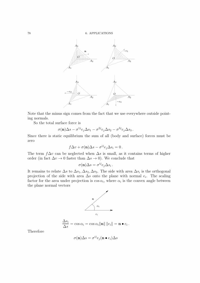
78 6. APPLICATIONS
−e1
−e2
−e3
O
O O
O
n
A1 A1
A1A1
A2
A2A2
A2
A3 A3
A3A3
Note that the minus sign comes from the fact that we use everywhere outside point-ing normals.
So the total surface force is
σ(n)∆s− σ1jej∆s1 − σ2jej∆s2 − σ3jej∆s3 .
Since there is static equilibrium the sum of all (body and surface) forces must bezero
f∆v + σ(n)∆s− σijej∆si = 0 .
The term f∆v can be neglected when ∆s is small, as it contains terms of higherorder (in fact ∆v → 0 faster than ∆s→ 0). We conclude that
σ(n)∆s = σijej∆si .
It remains to relate ∆s to ∆s1,∆s2,∆s3. The side with area ∆si is the orthogonalprojection of the side with area ∆s onto the plane with normal ei. The scalingfactor for the area under projection is cosαi, where αi is the convex angle betweenthe plane normal vectors
ei
n
αi
∆si∆s
= cosαi = cosαi‖n‖ ‖ei‖ = n • ei .
Therefore
σ(n)∆s = σijej(n • ei)∆s
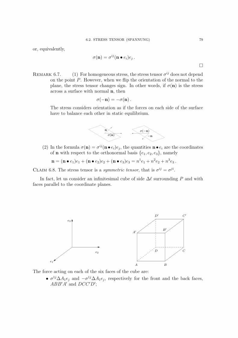
6.2. STRESS TENSOR (SPANNUNG) 79
or, equivalently,
σ(n) = σij(n • ei)ej .�
Remark 6.7. (1) For homogeneous stress, the stress tensor σij does not dependon the point P . However, when we flip the orientation of the normal to theplane, the stress tensor changes sign. In other words, if σ(n) is the stressacross a surface with normal n, then
σ(−n) = −σ(n) .The stress considers orientation as if the forces on each side of the surfacehave to balance each other in static equilibrium.
σ(n)
σ(−n)
−n
n
(2) In the formula σ(n) = σij(n• ei)ej , the quantities n• ei are the coordinatesof n with respect to the orthonormal basis {e1, e2, e3}, namely
n = (n • e1)e1 + (n • e2)e2 + (n • e3)e3 = n1e1 + n2e2 + n3e3 .
Claim 6.8. The stress tensor is a symmetric tensor, that is σij = σji.
In fact, let us consider an infinitesimal cube of side ∆ℓ surrounding P and withfaces parallel to the coordinate planes.
e1
e2
e3
A B
CD
A′B′
C′D′
The force acting on each of the six faces of the cube are:
• σ1j∆A1ej and −σ1j∆A1ej , respectively for the front and the back faces,ABB′A′ and DCC ′D′;

80 6. APPLICATIONS
• σ2j∆A2ej and −σ2j∆A2ej , respectively for the right and the left facesBCC ′B′ and ADD′A′;• σ3j∆A3ej and −σ3j∆A3ej, respectively for the top and the bottom facesABCD and A′B′C ′D′,
where ∆A1 = ∆A2 = ∆A3 = ∆s = (∆ℓ)2 is the common face area. We computenow the torque µ, assuming the forces are applied at the center of the faces (whosedistance is 1
2∆ℓ to the center point P ). Recall that the torque is the tendency of a
force to twist or rotate an object.
µ =∆ℓ
2e1 × σ1j∆s ej +
(−∆ℓ
2e1
)× (−σ1j∆s ej )
+∆ℓ
2e2 × σ2j∆s ej +
(−∆ℓ
2e2
)× (−σ2j∆s ej )
+∆ℓ
2e2 × σ3j∆s ej +
(−∆ℓ
2e3
)× (−σ3j∆s ej )
=∆ℓ∆s (ei × σijej) =
=∆ℓ∆s((σ23 − σ32)e1 + (σ31 − σ13)e2 + (σ12 − σ21)e3
).
Since the equilibrium is static, then L = 0, so that σij = σji.We can hence write
σ =
σ11 σ12 σ13
σ12 σ22 σ23
σ13 σ23 σ33
,
where the diagonal entries σ11, σ22 and σ33 are the normal components, that is thecomponents of the forces perpendicular to the coordinate planes and the remainingentries σ12, σ13 and σ23 are the shear components, that is the components of theforces parallel to the coordinate planes.
Since the stress tensor is symmetric, it can be orthogonally diagonalized, that is
σ =
σ1 0 00 σ2 00 0 σ3
,
where now σ1, σ2 and σ3 are the principal stresses, that is the eigenvalues of
σ. The eigenspaces of σ are the principal directions and the shear componentsdisappear for the principal planes.
6.2.1. Special forms of the stress tensor (written with respect to anorthonormal eigenbasis or another special basis).

6.2. STRESS TENSOR (SPANNUNG) 81
• Uniaxial stress with stress tensor given by
σ 0 00 0 00 0 0
Example 6.9. This is the stress tensor in a long vertical rod loaded byhanging a weight on the end.
• Plane stressed state or biaxial stress with stress tensor given byσ1 0 00 σ2 00 0 0
Example 6.10. This is the stress tensor in plate on which forces are appliedas in the picture.
• Pure shear with stress tensor given by
−σ 0 00 σ 00 0 0
or
0 σ 0σ 0 00 0 0
.(6.7)
This is special case of the biaxial stress, in the case in which σ1 = σ2. In(6.7) the first is the stress tensor written with respect to an eigenbasis, whilethe second is the stress tensor written with respect to an orthonormal basisobtained by rotating an eigenbasis by 45◦ about the third axis. In fact0 σ 0σ 0 00 0 0
=
√22
√22
0
−√22
√22
00 0 1
︸ ︷︷ ︸tL
−σ 0 00 σ 00 0 0
√22−
√22
0√22
√22
00 0 1
︸ ︷︷ ︸L
where L is the matrix of the change of coordinates.
• Shear deformation with stress tensor given by
0 σ12 σ13
σ12 0 σ23
σ13 σ23 0

82 6. APPLICATIONS
with respect to some orthonormal basis.
Fact 6.11. The stress tensor σ is a shear deformation if and only if its traceis zero.
Example 6.12. The stress tensor
2 −4 0−4 0 40 4 −2
represents a shear deformation. In fact one can check that
√22
0√22
0 1 0
−√22
0√22
︸ ︷︷ ︸tL
2 −4 0−4 0 40 4 −2
√22
0 −√22
0 1 0√22
0√22
︸ ︷︷ ︸L
=
0 0 −20 0 4
√2
−2 4√2 0
• Hydrostatic pressure with stress tensor given by−p 0 00 −p 00 0 −p
,
where p 6= 0 is the pressure. Here all eigenvalues are equal to −p.Example 6.13. Pressure of a fluid on a bubble.
Exercise 6.14. Any stress tensor can be written as the sum of a hydrostatic pressureand a shear deformation. Hint: look at the trace.
6.2.2. Contravariance of the stress tensor. Let B = {e1, e2, e3} and B ={e1, e2, e3} be two basis, and let
ei = Ljiej and ei = Λj
i ej ,(6.8)
where L := LBB is the matrix of the change of basis and Λ = L−1 is the inverse. Letn be a given unit vector and S the stress across a surface perpendicular to n. Then
S can be expressed in two way, respectively with respect to B and to BS = σij(n • ei)ej(6.9)
S = σij(n • ei)ej ,(6.10)
and we want to relate σij to σij. We start with the expression for S in (6.9) andrename the indices for later convenience.
S = σkm(n • ek)em = σkm(n • Λikei)(Λ
jmej) = σkmΛi
kΛjm(n • ei)ej ,
where in the second equality we used (6.8), and in the third we used linearity.Comparing the last expression with the expression in (6.10) we obtain
σij = σkmΛikΛ
jm ,
thus showing that σ is a contravariant 2-tensor or a tensor of type (0, 2).
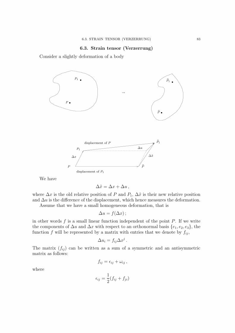
6.3. STRAIN TENSOR (VERZERRUNG) 83
6.3. Strain tensor (Verzerrung)
Consider a slightly deformation of a body
.
.
.
.
P
P
P1
P1
P
P
P1
P1
∆x ∆x
displacement of P1
displacement of P
∆u
We have
∆x = ∆x+∆u ,
where ∆x is the old relative position of P and P1, ∆x is their new relative positionand ∆u is the difference of the displacement, which hence measures the deformation.
Assume that we have a small homogeneous deformation, that is
∆u = f(∆x) ;
in other words f is a small linear function independent of the point P . If we writethe components of ∆u and ∆x with respect to an orthonormal basis {e1, e2, e3}, thefunction f will be represented by a matrix with entries that we denote by fij ,
∆ui = fij∆xj .
The matrix (fij) can be written as a sum of a symmetric and an antisymmetricmatrix as follows:
fij = ǫij + ωij ,
where
ǫij =1
2(fij + fji)
84 6. APPLICATIONS
is a symmetric matrix and is called the strain tensor or deformation tensor and
ωij =1
2(fij − fji)
is an antisymmetric matrix called the rotation tensor. We try to understand nowwhere these names come from.
Remark 6.15. First we verify that a (small) antisymmetric 3× 3 matrix representsa (small) rotation in 3-dimensional space.
Fact 6.16. Let V be a vector space with orthonormal basis B = {e1, e2, e3}, and let
ω =
abc
. The matrix of the linear map V → V defined by v 7→ ω× v with respect
to the basis B is
0 −c bc 0 −a−b a 0
.
In fact
ω × v =
abc
×
xyz
= det
e1 e2 e3a b cx y z
=
bz − cycx− azay − bx
=
0 −c bc 0 −a−b a 0
xyz
.
Note that the matrix (ωij) =
0 ω12 −ω13
−ω12 0 ω23
ω13 −ω23 0
corresponds to the cross
product with the vector ω =
−ω23
−ω13
−ω12
. �
The antisymmetric case. Suppose that the matrix (fij) was already antisymmet-
ric, so that
ωij = fij and ǫij = 0 .
By the Fact 6.16, the relation
∆ui = fij∆xj(6.11)
is equivalent to
∆u = ω ×∆x ,
so that
∆x = ∆x+∆u = ∆x+ ω ×∆x .

6.3. STRAIN TENSOR (VERZERRUNG) 85
When ω is small, this represents an infinitesimal rotation of an angle ‖ω‖ about theaxis Oω.
∆x ∆x
α
r
O
ω
In fact, since ω ×∆x is orthogonal to the plane determined by ω and by ∆x, itis tangent to the circle with center along the axis Oω and radius determined by ∆x.Moreover,
‖∆u‖ = ‖ω ×∆x‖ = ‖ω‖ ‖∆x‖ sinα︸ ︷︷ ︸r
,
and hence, since the length of an arc of a circle of radius r corresponding to an angleθ is rθ, infinitesimally this represents a rotation by an angle ‖ω.
The symmetric case. The opposite extreme case is when the matrix fij wasalready symmetric, so that
ǫij = fij and ωij = 0 .
We will see that it is ǫij that encodes the changes in the distances: in fact,
‖∆x‖2 = ∆x •∆x = (∆x+∆u) • (∆x+∆u)
= ∆x •∆x+ 2∆x •∆u+∆u •∆u≃ ‖∆x‖2 + 2ǫij∆x
i∆xj ,
(6.12)
where in the last step we neglected the term ‖∆u‖2 since it is small compared to∆u when ∆u→ 0 and used (6.11).
Remark 6.17. Even when fij is not purely symmetric, only the symmetric part ǫijis relevant for the distortion of the distances. In fact, if ωij is antisymmetric, the

86 6. APPLICATIONS
term 2ωij∆xi∆xj = 0, so that
‖∆x‖2 ≃ ‖∆x‖2 + 2fij∆xi∆xj = ‖∆x‖2 + 2ǫij∆x
i∆xj . �
Recall that a metric tensor (or inner product) encodes the distances amongpoints. It follows that a deformation changes the metric tensor. Let us denote byg the metric before the deformation and by g the metric after the deformation. Bydefinition we have
‖∆x‖2 def= g(∆x,∆x) = gij∆x
i∆xj = gij(∆xi +∆ui)(∆xj +∆uj)(6.13)
and
‖∆x‖2 def= g(∆x,∆x) = gij∆x
i∆xj .(6.14)
For infinitesimal deformations (that is if ∆u ∼ 0), (6.13) becomes
‖∆x‖2 = gij∆xi∆xj .
This, together with (6.14) and (6.12), leads to
gij∆xi∆xj ≃ gij∆x
i∆xj + 2ǫij∆xi∆xj
and hence
ǫij ≃1
2(gij − gij) ,
that is ǫij measures the change in the metric.By definition the strain tensor ǫij is symmetric
E =
ǫ11 ǫ12 ǫ13ǫ12 ǫ22 ǫ23ǫ13 ǫ23 ǫ33
,
where the terms on the diagonal (in green) determine the elongation or the contrac-tion of the body along the coordinate directions e1, e2, e3, and the terms above thediagonal (in orange) are the shear components of the strain tensor; that is ǫij isthe movement of a line element parallel to Oej towards Oei. Since it is a symmetrictensor it can be orthogonally diagonalized
ǫ1 0 00 ǫ2 00 0 ǫ3
,
The eigenvalues of E are the principal coefficients of the deformation and theeigenspaces are the principal directions of the deformation.

6.4. ELASTICITY TENSOR 87
6.3.1. Special forms of the strain tensor.
(1) Shear deformation when E is traceless
tr E = ǫ11 + ǫ22 + ǫ33 = 0 .
(2) Uniform compression when the principal coefficients of E are equal (andnonzero)
k 0 00 k 00 0 k
Exercise 6.18. Any strain tensor can be written as the sum of a uniformcompression and a shear deformation.
6.4. Elasticity tensor
The stress tensor represents an external exertion on the material, while the straintensor represents the material reaction to that exertion. In crystallography these arecalled field tensors because they represent imposed conditions, opposed to mattertensors, that represents material properties.
Hooke’s law says that, for small deformations, stress is related to strain by amatter tensor called elasticity tensor or stiffness tensor
σij = Eijkℓǫkl ,
while the tensor relating strain to stress is the compliance tensor
ǫkℓ = Sijkℓσij .
The elasticity tensor has rank 4, and hence in 3-dimensional space it has 34 = 81components. However symmetry reduces the number of independent componentsfor Eijkℓ.
(1) Minor symmetries: The symmetry of the stress tensor
σij = σji
implies that
Eijkℓ = Ejikℓ for each k, ℓ ;
it follows that for each k, ℓ fixed there are only 6 independent componentsEijkℓ
E11kℓ E12kℓ E13kℓ
E12kℓ E22kℓ E23kℓ
E13kℓ E23kℓ E33kℓ .
Having taken this in consideration, the number of independent componentsdecreases to 6 × 32 at the most. However the symmetry also of the straintensor
ǫkℓ = ǫℓk
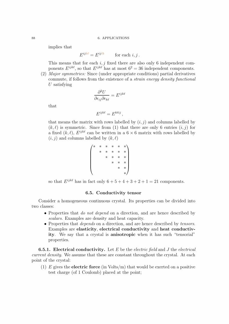
88 6. APPLICATIONS
implies that
Eijkℓ = Eijℓk for each i, j .
This means that for each i, j fixed there are also only 6 independent com-ponents Eijkℓ, so that Eijkℓ has at most 62 = 36 independent components.
(2) Major symmetries: Since (under appropriate conditions) partial derivativescommute, if follows from the existence of a strain energy density functional
U satisfying
∂2U
∂ǫij∂ǫkℓ= Eijkℓ
that
Eijkℓ = Ekℓij ,
that means the matrix with rows labelled by (i, j) and columns labelled by(k, ℓ) is symmetric. Since from (1) that there are only 6 entries (i, j) fora fixed (k, ℓ), Eijkℓ can be written in a 6 × 6 matrix with rows labelled by(i, j) and columns labelled by (k, ℓ)
∗ ∗ ∗ ∗ ∗ ∗∗ ∗ ∗ ∗ ∗∗ ∗ ∗ ∗∗ ∗ ∗∗ ∗∗
so that Eijkℓ has in fact only 6 + 5 + 4 + 3 + 2 + 1 = 21 components.
6.5. Conductivity tensor
Consider a homogeneous continuous crystal. Its properties can be divided intotwo classes:
• Properties that do not depend on a direction, and are hence described byscalars. Examples are density and heat capacity.• Properties that depends on a direction, and are hence described by tensors.Examples are elasticity, electrical conductivity and heat conductiv-ity. We say that a crystal is anisotropic when it has such “tensorial”properties.
6.5.1. Electrical conductivity. Let E be the electric field and J the electricalcurrent density. We assume that these are constant throughout the crystal. At eachpoint of the crystal:
(1) E gives the electric force (in Volts/m) that would be exerted on a positivetest charge (of 1 Coulomb) placed at the point;
6.5. CONDUCTIVITY TENSOR 89
(2) J (in Amperes/m2) gives the direction the charge carriers move and therate of electric current across an infinitesimal surface perpendicular tothat direction.
J is a function of E,
J = f(E) .
Consider a small increment ∆J in J caused by a small increment ∆E in E, and writethese increments in terms of their components with respect to a chosen orthonormalbasis {e1, e2, e3}.
∆J = ∆J iei and ∆E = ∆Eiei .
The increments are related by
∆J i =∂f i
∂Ej∆Ej + higher order terms in (∆Ej)2, (∆Ej)2, . . .
If the quantities ∆Ej are small, we can assume that
∆J i =∂f i
∂Ej∆Ej(6.15)
If we assume that ∂f i
∂Ej is independent of the point of the crystal,
∂f i
∂Ej= σi
j ∈ R
we obtain the relation
∆J i = σij∆E
j
or simply
∆J = σ∆E ,
where σ if the electrical conductivity tensor. This is a (1, 1)-tensor and maydepend4 on the initial value of E, that is the electrical conductivity may be differentfor small and large electric forces. If initially E = 0 and σ0 is the correspondingelectrical conductivity tensor, we obtain the relation
J = σ0E
that is called the generalized Ohm law. This is always under the assumption that∆E and ∆J are small and that the relation is linear.
The electrical resistivity tensor is
ρ = K−1 ,
that is, it is the (1, 1)-tensor such that
ρjiKℓj = δℓi .
4Typically if the dependence between E and J is linear for any value, and not only for smallones, the tensor ail not depend on the initial value of E.

90 6. APPLICATIONS
The electrical conductivity measures the material’s ability to conduct an electricalcurrent, while the electrical resistivity quantifies the ability of the material to opposethe flow of the electrical current.
For an isotropic crystal, all directions are equivalent and these tensors are spher-ical
σji = kδji and ρji =
1
kδji ,(6.16)
where k is a scalar, called the electrical conductivity of the crystal. Equa-tion (6.16) can also be written as
k 0 00 k 00 0 k
and
1k
0 00 1
k0
0 0 1k
.
In general, σji is neither symmetric nor antisymmetric (and actually symmetry does
not even make sense for a (1, 1) tensor unless a metric is fixed, since it does requirea canonical identification of V with V ∗).
6.5.2. Heat conductivity. Let T be the temperature and H the heat flux vec-
tor. For a homogeneous crystal and constant H and for a constant gradient of T ,Fourier heat conduction law says that
H = −K gradT .(6.17)
At each point of the crystal:
(1) gradT points in the direction of the highest ascent of the temperature andmeasures the rate of increase of T in that direction. The minus sign in (6.17)comes from the fact that the heat flows in the direction of the decreasingtemperature.
(2) H measure the amount of heat passing per unit area perpendicular to itsdirection per unit time.
Here K is the heat conductivity tensor or thermal conductivity tensor. Interms of components with respect to a chosen orthonormal basis
H i = −Kij(gradT )j .
Exercise 6.19. Verify that the gradient of a real function is a covariant 1-tensor.
The heat conductivity tensor is a contravariant 2-tensor and experiments showthat it is symmetric and hence can be orthogonally diagonalized. The heat resis-tivity tensor is
r = K−1 ,

6.5. CONDUCTIVITY TENSOR 91
and hence is also symmetric. With respect to an orthonormal basis, K is representedby
K1 0 00 K2 00 0 K3
,
where the eigenvalues of K are called the principal coefficients of heat conduc-tivity.
Physical considerations (that is the fact that heat flows always in the directionof decreasing temperature) show that the eigenvalues are positive
Ki > 0 .
The eigenspaces of K are called the principal directions of heat conductivity.

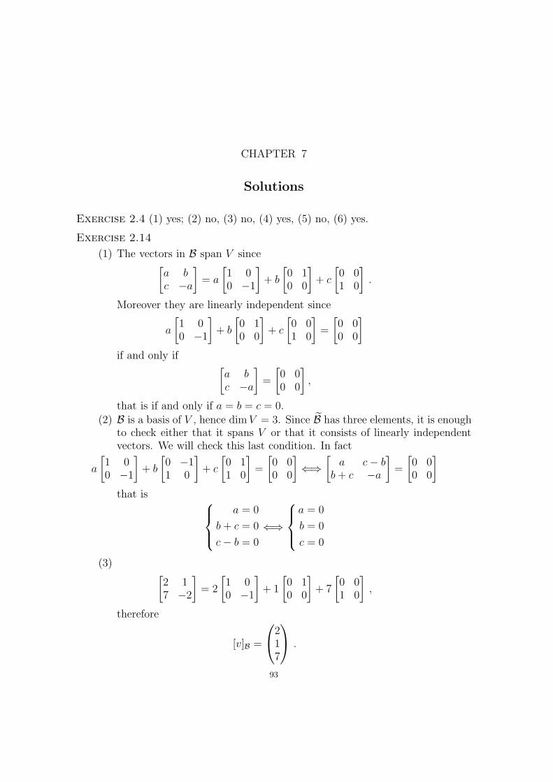
CHAPTER 7
Solutions
Exercise 2.4 (1) yes; (2) no, (3) no, (4) yes, (5) no, (6) yes.
Exercise 2.14
(1) The vectors in B span V since[a bc −a
]= a
[1 00 −1
]+ b
[0 10 0
]+ c
[0 01 0
].
Moreover they are linearly independent since
a
[1 00 −1
]+ b
[0 10 0
]+ c
[0 01 0
]=
[0 00 0
]
if and only if[a bc −a
]=
[0 00 0
],
that is if and only if a = b = c = 0.
(2) B is a basis of V , hence dimV = 3. Since B has three elements, it is enoughto check either that it spans V or that it consists of linearly independentvectors. We will check this last condition. In fact
a
[1 00 −1
]+ b
[0 −11 0
]+ c
[0 11 0
]=
[0 00 0
]⇐⇒
[a c− b
b+ c −a
]=
[0 00 0
]
that is
a = 0
b+ c = 0
c− b = 0
⇐⇒
a = 0
b = 0
c = 0
(3)[2 17 −2
]= 2
[1 00 −1
]+ 1
[0 10 0
]+ 7
[0 01 0
],
therefore
[v]B =
217
.
93
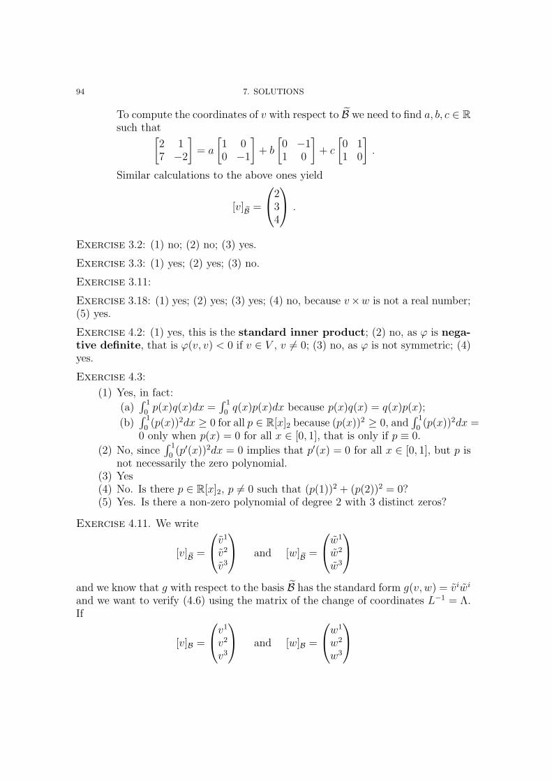
94 7. SOLUTIONS
To compute the coordinates of v with respect to B we need to find a, b, c ∈ R
such that[2 17 −2
]= a
[1 00 −1
]+ b
[0 −11 0
]+ c
[0 11 0
].
Similar calculations to the above ones yield
[v]B =
234
.
Exercise 3.2: (1) no; (2) no; (3) yes.
Exercise 3.3: (1) yes; (2) yes; (3) no.
Exercise 3.11:
Exercise 3.18: (1) yes; (2) yes; (3) yes; (4) no, because v×w is not a real number;(5) yes.
Exercise 4.2: (1) yes, this is the standard inner product; (2) no, as ϕ is nega-tive definite, that is ϕ(v, v) < 0 if v ∈ V , v 6= 0; (3) no, as ϕ is not symmetric; (4)yes.
Exercise 4.3:
(1) Yes, in fact:
(a)∫ 1
0p(x)q(x)dx =
∫ 1
0q(x)p(x)dx because p(x)q(x) = q(x)p(x);
(b)∫ 1
0(p(x))2dx ≥ 0 for all p ∈ R[x]2 because (p(x))
2 ≥ 0, and∫ 1
0(p(x))2dx =
0 only when p(x) = 0 for all x ∈ [0, 1], that is only if p ≡ 0.
(2) No, since∫ 1
0(p′(x))2dx = 0 implies that p′(x) = 0 for all x ∈ [0, 1], but p is
not necessarily the zero polynomial.(3) Yes(4) No. Is there p ∈ R[x]2, p 6= 0 such that (p(1))2 + (p(2))2 = 0?(5) Yes. Is there a non-zero polynomial of degree 2 with 3 distinct zeros?
Exercise 4.11. We write
[v]B =
v1
v2
v3
and [w]B =
w1
w2
w3
and we know that g with respect to the basis B has the standard form g(v, w) = viwi
and we want to verify (4.6) using the matrix of the change of coordinates L−1 = Λ.If
[v]B =
v1
v2
v3
and [w]B =
w1
w2
w3

7. SOLUTIONS 95
then we have that v1
v2
v3
= Λ
v1
v2
v3
=
v1 − v2v2 − v3v3
and w1
w2
w3
= Λ
w1
w2
w3
=
w1 − w2
w2 − w3
w3
It follows that
g(v, w) = viwi = (v1 − v2)(w1 − w2) + (v2 − v3)(w2 − w3) + v3w3
= v1w1 − v1w2 − v2w1 + 2v2w2 − v2w3 − w3v2 + 2v3w3 .
Exercise 4.14 With respect to B, we have
‖v‖ = (12 + 12 + 12)1/2 =√3
‖w‖ = ((−1)2 + (−1)2 + 32)1/2 =√11
and with respect to E‖v‖ = (3 · 3− 3 · 2− 2 · 3 + 2 · 2 · 2− 2 · 1− 1 · 2 + 2 · 1 · 1)1/2 =
√3
‖w‖ = (1 · 1− 1 · 2− 2 · 1 + 2 · 2 · 2− 2 · 3− 3 · 2 + 2 · 3 · 3)1/2 =√11 .
Exercise: 4.25. Saying that the orthogonality is meant with respect to g, meansthat we have to show that g(v − projbkv, bk) = 0. In fact,
g(v − projbkv, bk) = g(v − g(v, bk)
g(bk, bk)bk, bk) = g(v, bk)−
g(v, bk)
✘✘✘✘✘g(bk, bk)
✘✘✘✘✘g(bk, bk) = 0