Multilingual Spoken Term Detection: Finding and Testing New

Pronunciations

Richard Sproat, Jim Baker, Martin Jansche, Bhuvana Ramabhadran,Michael Riley, Murat Saraclar, Abhinav Sethy, Patrick Wolfe, Sanjeev Khudanpur, Arnab Ghoshal,

Kristy Hollingshead, Chris White, Ting Qian, Erica Cooper, Morgan Ulinski

c©2008, The Authors

Contents

1 Abstract 1

2 Web-Derived Pronunciations 32.1 Introduction . . . . . . . . . . . . . . . . . . . . . . . . . . . . . . . . . . . . . . . . . . . . . . 32.2 Pronunciation Extraction . . . . . . . . . . . . . . . . . . . . . . . . . . . . . . . . . . . . . . 3

2.2.1 IPA Pronunciation Extraction . . . . . . . . . . . . . . . . . . . . . . . . . . . . . . . . 42.2.2 Ad-hoc Pronunciation Extraction . . . . . . . . . . . . . . . . . . . . . . . . . . . . . . 4

2.3 Pronunciation Extraction Validation . . . . . . . . . . . . . . . . . . . . . . . . . . . . . . . . 42.4 Pronunciation Normalization . . . . . . . . . . . . . . . . . . . . . . . . . . . . . . . . . . . . 5

2.4.1 IPA Pronunciation Normalization . . . . . . . . . . . . . . . . . . . . . . . . . . . . . . 62.4.2 Ad-hoc Pronunciation Normalization . . . . . . . . . . . . . . . . . . . . . . . . . . . . 8

2.5 Conclusion . . . . . . . . . . . . . . . . . . . . . . . . . . . . . . . . . . . . . . . . . . . . . . 9

3 Interscriptal Transcription 113.1 Introduction . . . . . . . . . . . . . . . . . . . . . . . . . . . . . . . . . . . . . . . . . . . . . . 113.2 Previous Work . . . . . . . . . . . . . . . . . . . . . . . . . . . . . . . . . . . . . . . . . . . . 133.3 Overview of deliverables . . . . . . . . . . . . . . . . . . . . . . . . . . . . . . . . . . . . . . . 153.4 String Distances for Interscriptal Transcription . . . . . . . . . . . . . . . . . . . . . . . . . . 15

3.4.1 Framework . . . . . . . . . . . . . . . . . . . . . . . . . . . . . . . . . . . . . . . . . . 163.4.1.1 Data . . . . . . . . . . . . . . . . . . . . . . . . . . . . . . . . . . . . . . . . 163.4.1.2 Language Representation . . . . . . . . . . . . . . . . . . . . . . . . . . . . . 163.4.1.3 Discriminative Modeling Using Perceptron . . . . . . . . . . . . . . . . . . . 17

3.4.2 Experimental Results . . . . . . . . . . . . . . . . . . . . . . . . . . . . . . . . . . . . 183.4.2.1 Accuracy of Models for English-Chinese Transcription . . . . . . . . . . . . . 193.4.2.2 Effect of Training Size . . . . . . . . . . . . . . . . . . . . . . . . . . . . . . . 193.4.2.3 Using Negative Neighbors as Negative Examples . . . . . . . . . . . . . . . . 21

3.4.3 Extensibility . . . . . . . . . . . . . . . . . . . . . . . . . . . . . . . . . . . . . . . . . 213.5 Score Combination for Matching Transliteration Pairs . . . . . . . . . . . . . . . . . . . . . . 23

3.5.1 Introduction . . . . . . . . . . . . . . . . . . . . . . . . . . . . . . . . . . . . . . . . . 233.5.2 Methodology . . . . . . . . . . . . . . . . . . . . . . . . . . . . . . . . . . . . . . . . . 23

3.5.2.1 Orthographic Match . . . . . . . . . . . . . . . . . . . . . . . . . . . . . . . . 243.5.2.2 Phonetic Match . . . . . . . . . . . . . . . . . . . . . . . . . . . . . . . . . . 243.5.2.3 Temporal Distributional Similarity . . . . . . . . . . . . . . . . . . . . . . . . 253.5.2.4 Perceptron Classifier . . . . . . . . . . . . . . . . . . . . . . . . . . . . . . . . 253.5.2.5 Score Combination . . . . . . . . . . . . . . . . . . . . . . . . . . . . . . . . . 26

3.5.3 Experimental Setup . . . . . . . . . . . . . . . . . . . . . . . . . . . . . . . . . . . . . 273.5.4 Results: Ranking . . . . . . . . . . . . . . . . . . . . . . . . . . . . . . . . . . . . . . . 273.5.5 Results: Classification . . . . . . . . . . . . . . . . . . . . . . . . . . . . . . . . . . . . 283.5.6 Discussion & Future Work . . . . . . . . . . . . . . . . . . . . . . . . . . . . . . . . . . 29

3.6 ScriptTranscriber . . . . . . . . . . . . . . . . . . . . . . . . . . . . . . . . . . . . . . . . . 293.7 Ongoing Work . . . . . . . . . . . . . . . . . . . . . . . . . . . . . . . . . . . . . . . . . . . . 34

v

4 Multilingual Spoken Term Detection 354.1 Part I - Effect of Pronunciations on OOV Queries in Spoken Term Detection . . . . . . . . . 35

4.1.1 Introduction . . . . . . . . . . . . . . . . . . . . . . . . . . . . . . . . . . . . . . . . . 354.1.2 Methods . . . . . . . . . . . . . . . . . . . . . . . . . . . . . . . . . . . . . . . . . . . . 36

4.1.2.1 WFST-based Spoken Term Detection . . . . . . . . . . . . . . . . . . . . . . 364.1.2.2 Query Forming and Expansion for Phonetic Search . . . . . . . . . . . . . . 37

4.1.3 Experiments . . . . . . . . . . . . . . . . . . . . . . . . . . . . . . . . . . . . . . . . . 394.1.3.1 Experimental Setup . . . . . . . . . . . . . . . . . . . . . . . . . . . . . . . . 394.1.3.2 Results . . . . . . . . . . . . . . . . . . . . . . . . . . . . . . . . . . . . . . . 39

4.1.4 Pronunciations derived from the web . . . . . . . . . . . . . . . . . . . . . . . . . . . . 414.1.5 Use of a foriegn language: Turkish . . . . . . . . . . . . . . . . . . . . . . . . . . . . . 424.1.6 Part I - Summary . . . . . . . . . . . . . . . . . . . . . . . . . . . . . . . . . . . . . . 43

4.2 Part II - Unsupervised pronunciation validation . . . . . . . . . . . . . . . . . . . . . . . . . . 434.2.1 Introduction . . . . . . . . . . . . . . . . . . . . . . . . . . . . . . . . . . . . . . . . . 43

4.2.1.1 Baseline Supervised Method . . . . . . . . . . . . . . . . . . . . . . . . . . . 444.2.1.2 Data set, OOV terms, systems . . . . . . . . . . . . . . . . . . . . . . . . . . 454.2.1.3 Supervised validation . . . . . . . . . . . . . . . . . . . . . . . . . . . . . . . 45

4.2.2 Unsupervised Method . . . . . . . . . . . . . . . . . . . . . . . . . . . . . . . . . . . . 454.2.3 Results . . . . . . . . . . . . . . . . . . . . . . . . . . . . . . . . . . . . . . . . . . . . 46

4.2.3.1 Large vocabulary continuous speech recognition . . . . . . . . . . . . . . . . 464.2.3.2 Spoken term detection . . . . . . . . . . . . . . . . . . . . . . . . . . . . . . . 47

4.2.4 Part II - Summary . . . . . . . . . . . . . . . . . . . . . . . . . . . . . . . . . . . . . . 484.3 Conclusion . . . . . . . . . . . . . . . . . . . . . . . . . . . . . . . . . . . . . . . . . . . . . . 48

5 Acknowledgments 49

vi

List of Figures

2.1 Precision vs. recall in pronunciation extraction validation. . . . . . . . . . . . . . . . . . . . . 52.2 Cross-validation results by website. . . . . . . . . . . . . . . . . . . . . . . . . . . . . . . . . . 72.3 Effect of pronunciation normalization – L2P models trained using normalized web data are

better at predicting the reference pronunciations. . . . . . . . . . . . . . . . . . . . . . . . . . 82.4 Performance on rare words – normalized web pronunciations help a lot on rare words. . . . . 9

3.1 Some automatically found n-tuples of transcriptions mined from the Web. . . . . . . . . . . . . . . 123.2 Some automatically found pairs of transcriptions mined from the Web. . . . . . . . . . . . . . . . . 133.3 Temporal cooccurrence of the placenames Nunavut and Aglukkaq in English and Inuktitut in the

Nunavut Hansards. . . . . . . . . . . . . . . . . . . . . . . . . . . . . . . . . . . . . . . . . . . . 143.4 In the model of English letters and Chinese phonemic transcription (Worldbet), performance

increases as a function of training size. . . . . . . . . . . . . . . . . . . . . . . . . . . . . . . . 203.5 Increase of training size correlates with increase of performance in general. . . . . . . . . . . . 203.6 Model trained with negative neighbors performed poorly. . . . . . . . . . . . . . . . . . . . . 213.7 Discriminating English-Korean transcription pairs using English letters and Worldbet symbols

for Korean. . . . . . . . . . . . . . . . . . . . . . . . . . . . . . . . . . . . . . . . . . . . . . . 223.8 Discriminating English-Korean transcription pairs using English letters and Worldbet symbols

for Arabic. . . . . . . . . . . . . . . . . . . . . . . . . . . . . . . . . . . . . . . . . . . . . . . . 223.9 Examples of English/foreign transcription pairs, shown here with their pronunciations in each language. 243.10 Examples of the distributional similarity of the occurrences over time of English terms with their

transcription pairs in both Chinese and Arabic. ∗Indicates a correct pairing. . . . . . . . . . . . . . 263.11 Examples of the best-matched transcription pairs according to the phonetic-match approach and a

temporal correlation–match approach. Only the term marked by an ∗ is a correct match. . . . . . . 273.12 XML document structure for ScriptTranscriber. . . . . . . . . . . . . . . . . . . . . . . . . . . 303.13 Interactive use of the ScriptTranscriber tools. . . . . . . . . . . . . . . . . . . . . . . . . . . . . 34

4.1 Index structures . . . . . . . . . . . . . . . . . . . . . . . . . . . . . . . . . . . . . . . . . . . 364.2 Comparison of 1-pass & 2-pass strategies in terms of retrieval performance and runtime . . . 384.3 ATWV vs N-best L2S Pronunciations . . . . . . . . . . . . . . . . . . . . . . . . . . . . . . . 404.4 Combined DET plot for weighted L2S pronunciations . . . . . . . . . . . . . . . . . . . . . . 404.5 English results: Pairwise union of Pronunciations . . . . . . . . . . . . . . . . . . . . . . . . . 424.6 English results: Subword indexing using various pronunciations . . . . . . . . . . . . . . . . . 434.7 DET curve on Turkish audio . . . . . . . . . . . . . . . . . . . . . . . . . . . . . . . . . . . . 434.8 Phone Error Rate w.r.t. reference lexicon . . . . . . . . . . . . . . . . . . . . . . . . . . . . . 474.9 STD DET Curves . . . . . . . . . . . . . . . . . . . . . . . . . . . . . . . . . . . . . . . . . . 47

vii

List of Tables

2.1 Ad-hoc pronunciation extraction patterns and counts. . . . . . . . . . . . . . . . . . . . . . . 42.2 Phoneme error rates (in %) for 5-fold cross validation on the intersection between Pronlex

and Web-IPA pronunciations. . . . . . . . . . . . . . . . . . . . . . . . . . . . . . . . . . . . . 6

3.1 Examples of features and associated costs. Pseudofeatures are shown in boldface. Excep-tional denotes a situation such as the semivowel [j] substituting for the affricate [dZ]. Substi-tutions between these two sounds actually occur frequently in second-language error data. . . 12

3.2 Worldbet as a phonetic representation of Chinese characters. . . . . . . . . . . . . . . . . . . 173.3 Model accuracy on positive and negative test cases, and its overall performance, compared to

the model based on phonetic features as well as the baseline (a blind model). . . . . . . . . . 193.4 Results on ranking English-Chinese or English-Arabic transcription pairs, mined from comparable

corpora. Top three rows are single-score results; bottom four rows are linear-combination results.

MRR: Mean reciprocal-rank. . . . . . . . . . . . . . . . . . . . . . . . . . . . . . . . . . . . . . . 283.5 True-positive matrices on classifying English-Chinese or English-Arabic transcription pairs as either

valid (“positive”) or invalid (“negative”) pairs. . . . . . . . . . . . . . . . . . . . . . . . . . . . . 29

4.1 Reflex Results . . . . . . . . . . . . . . . . . . . . . . . . . . . . . . . . . . . . . . . . . . . . 394.2 Best Performing N-best L2S Pronunciations . . . . . . . . . . . . . . . . . . . . . . . . . . . . 404.3 S2S N-best Pronunciations expanding L2S output . . . . . . . . . . . . . . . . . . . . . . . . . 414.4 Number of OOVs that had pronunciations on the web . . . . . . . . . . . . . . . . . . . . . . 414.5 English results:Analysis of L2S v/s Web-based pronunciations with positive impact . . . . . . 424.6 English results:Analysis of L2S v/s Web-based pronunciations with negative impact . . . . . 424.7 Example pronunciations and PER . . . . . . . . . . . . . . . . . . . . . . . . . . . . . . . . . 464.8 LVCSR WER . . . . . . . . . . . . . . . . . . . . . . . . . . . . . . . . . . . . . . . . . . . . . 47

viii

Chapter 1

Abstract

When you listen to the evening news, or read a newspaper, book or web site, there is a good chance thatyou will hear or see a term — perhaps a name, perhaps a technical term — that you have never seen before.Such words are often novel or rare and are often names (of people, places, organizations. . . ). They are hardfor humans to process, but they are even harder for automatic speech and language processing systems.

For a single language, a speech recognition or text-to-speech system needs to know how to pronounce aword to recognize or say it. For two languages, in particular a pair with different writing systems, a searchengine or document summarizer needs to know how to transcribe one word to another to retrieve or distillacross languages. For example, the soccer player written in English text as Maciej Zurawski would appearas 마치에이주라브스키 (ma-chi-e-i ju-ra-beu-seu-ki) in Korean

In this project we attack both problems – unusual term pronunciation and term transcription. Forpronunciation, we make use of the huge numbers of pronunciations that are now available in various formson the web to mine pronunciations. This ranges from straightforward, such as dictionary sites and Wikipediaentries where people use a fairly strict phonetic transcription system such as IPA, to difficult such as:

• Trio Shares Nobel Prize in Medicine – The Nobel is a particularly striking achievement for Capecchi(pronounced kuh-PEK’-ee).

Here we need to look in the vicinity of the name “Capecchi” to find the pronunciation, make use of theword “pronounced”, and then interpret the writer’s attempt to render the pronunciation using an English-based ad-hoc “phonetic” orthography. The problem is therefore one of entity extraction, where the entitiesto extract can be either relatively easy or relatively hard. A relatively easy case is Wikipedia, which usesstandard IPA transcriptions that are clearly delimited by markup. On general web pages, tokens withUnicode IPA characters are potential pronunciations. Data extracted from Wikipedia can be matchedagainst these tokens to provide training material for entity extraction. Statistical entity extractors for themore difficult case of ad-hoc phonetic transcriptions (such as “kuh-PEK’-ee” above) can be bootstrappedfrom unannotated web pages containing patterns such as “pronounced as”. These entity extractors make useof both the textual environment and the letter-to-sound constraints between the candidate pronunciationand its corresponding orthography.

We also use speech data to test possible pronunciation variants by comparing the performance of spokenterm detection systems using these different variants. Pronunciations mined from the web are used to suggestpronunciations for spoken term detection; transcription are used to suggest reasonable candidates to searchfor in a speech stream in another language. We use a novel technique called delayed-decision testing to testcandidate pronunciations in speech, and to choose the best one from a set of candidates via a sequentialtesting procedure, with the associated null hypothesis stating that all candidate pronunciations exhibit thesame performance on average. Spoken term detection are in turn used for automatic labeling of practicedata acquired to test this null hypothesis; however, this automatic labeling procedure inevitably inducesfalse alarms as well as correct detections. Delayed-decision testing are then used to choose the correctpronunciation in spite of these false alarms, leading to improved pronunciations for newly identified terms.

For transcription, we use available resources – dictionaries, and text corpora – as well as methods for pho-netic matching across scripts and tracking names across time in comparable corpora (such as news sources).

1

In previous work at UIUC, JHU and many other sites, people have investigated phonetic transcription modelstrained from lexicons. More recently, we have developed techniques to guess transcription equivalents usingpronunciation estimates for English terms, pronunciation guesses for the foreign term, and phonetic distancesbased upon standard phonetic features as well as “pseudofeatures” based on phonetic substitutions observedin second-language learners of English. Reasonable transcription matches can be found using hand-tunedcosts based on these features, though improved performance can be demonstrated by discriminative trainingof the weights on even a short dictionary of transcriptions. We have also investigated using time correlationsof terms across comparable corpora, such as newswire text. Related terms, including transcriptions of thesame name, distribute similarly in time, and this is powerful additional evidence over and above phoneticsimilarity.

2

Chapter 2

Web-Derived Pronunciations

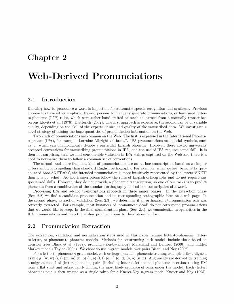
2.1 Introduction

Knowing how to pronounce a word is important for automatic speech recognition and synthesis. Previousapproaches have either employed trained persons to manually generate pronunciations, or have used letter-to-phoneme (L2P) rules, which were either hand-crafted or machine-learned from a manually transcribedcorpus Elovitz et al. (1976); Dietterich (2002). The first approach is expensive, the second can be of variablequality, depending on the skill of the experts or size and quality of the transcribed data. We investigate anovel strategy of mining the huge quantities of pronunciation information on the Web.

Two kinds of pronunciations are common on the Web: The first is expressed in the International PhoneticAlphabet (IPA), for example ‘Lorraine Albright /Ol braIt/’. IPA pronunciations use special symbols, suchas ‘O’, which can unambiguously denote a particular English phoneme. However, there are no universallyaccepted conventions for transcribing pronunciations in IPA, and the use of IPA requires some skill. It isthen not surprising that we find considerable variation in IPA strings captured on the Web and there is aneed to normalize them to follow a common set of conventions.

The second, and more frequent, kind of pronunciations use an ad-hoc transcription based on a simpleror less ambiguous spelling than standard English orthography. For example, when we see ‘bruschetta (pro-nounced broo-SKET-uh)’, the intended pronunciation is more intuitively represented by the letters ‘SKET’than it is by ‘schet’. Ad-hoc transcriptions follow the rules of English orthography and do not require anyspecialized skills. However, they do not provide a phonemic transcription, so one of our tasks is to predictphonemes from a combination of the standard orthography and ad-hoc transcription of a word.

Processing IPA and ad-hoc transcriptions proceeds in three major phases. In the extraction phase(Sec. 2.2) we find a candidate pronunciation and its corresponding orthographic form on a web page. Inthe second phase, extraction validation (Sec. 2.3), we determine if an orthography/pronunciation pair wascorrectly extracted. For example, most instances of ‘pronounced dead’ do not correspond pronunciationsthat we would like to keep. In the final normalization phase (Sec. 2.4), we canonicalize irregularities in theIPA pronunciations and map the ad-hoc pronunciations to their phonemic form.

2.2 Pronunciation Extraction

The extraction, validation and normalization steps used in this paper require letter-to-phoneme, letter-to-letter, or phoneme-to-phoneme models. Methods for constructing such models include those based ondecision trees Black et al. (1998), pronunciation-by-analogy Marchand and Damper (2000), and hiddenMarkov models Taylor (2005). We chose to use n-gram models over pairs Bisani and Ney (2002).

For a letter-to-phoneme n-gram model, each orthographic and phonemic training example is first aligned,as in e.g. (w, w) (i, i) (m, m) (b, b) (–, @) (l, l) (e, –) (d, d) (o, @) (n, n). Alignments are derived by traininga unigram model of (letter, phoneme) pairs (including letter deletions and phoneme insertions) using EMfrom a flat start and subsequently finding the most likely sequence of pairs under the model. Each (letter,phoneme) pair is then treated as a single token for a Kneser-Ney n-gram model Kneser and Ney (1995).

3

Type Pattern Countparen \(pronounced (as |like )?([^)]+)\) 3415Kquote pronounced (as |like )?"([^"]+)" 835K

comma , pronounced (as |like )?([^,]+), 267K

Table 2.1: Ad-hoc pronunciation extraction patterns and counts.

Once built, the n-gram model is represented as a weighted finite-state transducer (FST), mapping lettersto phonemes, using the OpenFst Library Allauzen et al. (2007), which allows easy implementation of theoperations that follow.

Our pronunciations are extracted from Google’s web and news page repositories. The pages are restrictedto those that Google has classified as in English and from non-EU countries. The extraction of IPA and ofad-hoc pronunciations uses different techniques.

2.2.1 IPA Pronunciation Extraction

The Unicode representation of most English words in IPA requires characters outside the ASCII range. Forinstance, only 3.8% to 8.6% (depending on transcription conventions) of the words in the 100K Pronlexdictionary1 have completely ASCII-representable IPA pronunciations (e.g., ‘beet’ /bit/). Most of the non-ASCII characters are drawn from the Unicode IPA extension range (0250–02AF), which are easily identifiedon web pages. Our candidate IPA pronunciations consist of web terms2 that are composed entirely of legalEnglish IPA characters, that have at least one non-ASCII character, and that are delimited by a pair offorward slashes (‘/ . . . /’), back slashes (‘\ . . . \’), or square brackets (‘[. . .]’).

Once these candidate IPA pronunciations are identified, the corresponding orthographic terms are nextsought. To do so, an English phoneme-to-letter model, Pr[λ|π], which estimates the probability that anorthographic string λ corresponds to a given phonemic string π, is used. First, a unigram letter-phonemejoint model, Pru[λ, π], is trained on the Pronlex dictionary using the method described above. We use aunigram model both to ensure wide generalization and to make it likely that the subsequent results do notdepend greatly on the bootstrap English dictionary. With this model in hand, we extract that contiguoussequence of terms λ, among the preceding twenty terms to each candidate pronunciation π, that maximizesPr[λ|π] = Pru[λ, π]/Σλ Pru[λ, π]. We found 2.53M candidate orthographic and phonemic string pairs (309Kunique pairs) in this way. These are then passed to extraction validation in Sec. 2.3.

2.2.2 Ad-hoc Pronunciation Extraction

Ad-hoc pronunciations are identified by matches to the regular expressions indicated in Table 2.1. Tofind the corresponding conventionally-spelled terms, an English letter-to-letter model, Pr[λ2|λ1], whichestimates the probability that the conventionally-spelled string λ2 corresponds to a given ad-hoc pro-nunciation string λ1, is used. Assuming that λ1 and λ2 are independent given their underlying phone-mic pronunciation π, Pr[λ2 |λ1] =

∑π Pr[λ2 |π] Pr[π |λ1] (implemented by weighted FST composition).

Given the unigram model Pru[λ, π] of Sec. 2.2.1, the estimates Pr[λ2|π] = Pru[λ2, π]/Σλ Pru[λ, π] andPr[π|λ1] = Pru[λ1, π]/Σπ Pru[λ1, π] are used.

We then extract that contiguous sequence of terms λ2, among the preceding eight terms to each candidatepronunciation λ1, that maximizes Pr[λ2|λ1]. We found 4.52M candidate orthographic and phonemic stringpairs (568K unique pairs) with pair counts for specific patterns indicated in Table 2.1. These pairs are thenpassed to extraction validation described in the next section.

2.3 Pronunciation Extraction Validation

Once extraction has taken place, a validation step is applied to judge whether the items extracted arecorrect in the sense that they find each orthographic term and the corresponding pronunciation providedword-for-word. We began by annotating 667 randomly-selected (orthography, IPA pronunciation) pairs and

1CALLHOME American English Lexicon, LDC97L20.2By terms we mean tokens exclusive of punctuation and HTML markup.

4

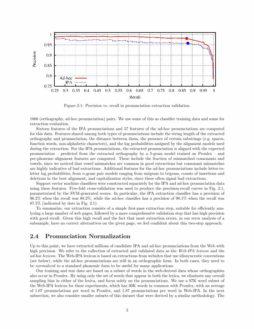
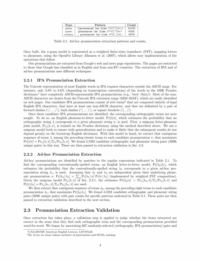
Figure 2.1: Precision vs. recall in pronunciation extraction validation.

1000 (orthography, ad-hoc pronunciation) pairs. We use some of this as classifier training data and some forextraction evaluation.

Sixteen features of the IPA pronunciations and 57 features of the ad-hoc pronunciations are computedfor this data. Features shared among both types of pronunciations include the string length of the extractedorthography and pronunciation, the distance between them, the presence of certain substrings (e.g. spaces,function words, non-alphabetic characters), and the log probabilities assigned by the alignment models usedduring the extraction. For the IPA pronunciations, the extracted pronunciation is aligned with the expectedpronunciation – predicted from the extracted orthography by a 5-gram model trained on Pronlex – andper-phoneme alignment features are computed. These include the fraction of mismatched consonants andvowels, since we noticed that vowel mismatches are common in good extractions but consonant mismatchesare highly indicative of bad extractions. Additional features for the ad-hoc pronunciations include letter-to-letter log probabilities, from n-gram pair models ranging from unigram to trigram, counts of insertions anddeletions in the best alignment, and capitalization styles, since these often signal bad extractions.

Support vector machine classifiers were constructed separately for the IPA and ad-hoc pronunciation datausing these features. Five-fold cross-validation was used to produce the precision-recall curves in Fig. 2.1,parameterized by the SVM-generated scores. In particular, the IPA extraction classifier has a precision of96.2% when the recall was 88.2%, while the ad-hoc classifier has a precision of 98.1% when the recall was87.5% (indicated by dots in Fig. 2.1).

To summarize, our extraction consists of a simple first-pass extraction step, suitable for efficiently ana-lyzing a large number of web pages, followed by a more comprehensive validation step that has high precisionwith good recall. Given this high recall and the fact that most extraction errors, in our error analysis of asubsample, have no correct alternatives on the given page, we feel confident about this two-step approach.

2.4 Pronunciation Normalization

Up to this point, we have extracted millions of candidate IPA and ad-hoc pronunciations from the Web withhigh precision. We refer to the collection of extracted and validated data as the Web-IPA lexicon and thead-hoc lexicon. The Web-IPA lexicon is based on extractions from websites that use idiosyncratic conventions(see below), while the ad-hoc pronunciations are still in an orthographic form. In both cases, they need tobe normalized to a standard phonemic form to be useful for many applications.

Our training and test data are based on a subset of words in the web-derived data whose orthographiesalso occur in Pronlex. By using only the set of words that appear in both the lexica, we eliminate any overallsampling bias in either of the lexica, and focus solely on the pronunciations. We use a 97K word subset ofthe Web-IPA lexicon for these experiments, which has 30K words in common with Pronlex, with an averageof 1.07 pronunciations per word in Pronlex, and 1.87 pronunciations per word in Web-IPA. In the nextsubsection, we also consider smaller subsets of this dataset that were derived by a similar methodology. The

5

training data for ad-hoc normalization was augmented by words whose pronunciations could be assembledfrom hyphenated portions of the ad-hoc transcription (e.g. if the ad-hoc transcription of ‘Circe’ is ‘Sir-see’,we look up the Pronlex phonemic transcriptions of ‘sir’ and ‘see’).

Some of our test sets, further described below, are drawn at random from the 30K Pronlex/Web-IPAlexicon. For others, we set aside rare words as test data, chosen by low counts in the HUB4 Broadcast Newscorpora. We are interested in rare words because they are less likely to occur in existing lexica. Handlingthese otherwise out-of-vocabulary (OOV) words is important in many applications.

We evaluate pronunciations by aligning a predicted phoneme string with a reference and computing thephoneme error rate (PhER) – analogous to word error rate in automatic speech recognition – as the numberof insertions, deletions, and substitutions divided by the number of phonemes in the reference (times 100%).In cases of multiple predicted or reference pronunciations, the pair with the lowest PhER is chosen.

2.4.1 IPA Pronunciation Normalization

We first compare the quality of the Web-IPA lexicon with Pronlex, by performing 5-fold cross-validation ex-periments on their orthographic intersection described above. For each cross-validation run, two L2P modelsare trained on the same 24K subset of the intersection – one using the Pronlex pronunciations, and the otherusing the Web-IPA pronunciations. Each of the models is then used to generate candidate pronunciationsfor the same 6K subset left out of the training. The two sets of generated candidate pronunciations are thenscored against the test pronunciations from both lexica, giving us four PhER numbers. The overall PhERfor these four cases are shown in Table 2.2.

PPPPPPPPTestTrain Pronlex Web-IPA

Pronlex 6.35 17.10Web-IPA 14.33 12.98

Table 2.2: Phoneme error rates (in %) for 5-fold cross validation on the intersection between Pronlex andWeb-IPA pronunciations.

At a first glance the PhER numbers presented in Table 2.2 may suggest that the Web-IPA data isinherently of lower quality. But a very different picture emerges when one breaks down these PhER numbersby individual websites. We repeated the above cross-validation experiments, but instead using the entireWeb-IPA data, the orthographic intersection was done using data collected from individual websites. Fig. 2.2shows the same four PhER numbers for 7 of the 10 websites with the most extracted pronunciations. Wenotice that for several websites, L2P models trained using the web pronunciations are almost as good atpredicting the website pronunciations (red bars) as a model trained on Pronlex is at predicting Pronlexpronunciations (dark blue bars). However, in all cases, models trained on web data are poor predictors ofPronlex data, and vice versa.

These experiments demonstrate that websites vary in the quality of pronunciations available from them.Moreover, the websites list different pronunciations than what one would obtain from Pronlex. The differ-ences can be caused both by improper use of IPA symbols, as well as other site-specific conventions. Forinstance, ‘graduate’ is pronounced as either /gôædZuIt/ or /gôædZueIt/ in Pronlex, but appears as /gôad-

jUeIt/, /gôædjUIt/, /gôædju@t/, /gôædjuIt/, and /gôædZU@t/ among the ten most frequent websites.Site-specific normalization The considerable variability of pronunciations across websites strongly

motivate the need for a site-specific normalization of the pronunciations to a more site-neutral target form.Here we use Pronlex as our target. As before, we find the orthographic intersection of the lexicon obtainedfrom a website and Pronlex. If multiple pronunciations are present, then the two with the smallest phonemeedit distance are selected. Using these pronunciation pairs we train a phoneme-to-phoneme (P2P) trans-duction model, which takes a pronunciation obtained from the website and converts it to a Pronlex-likeform.

The model for the P2P normalizing transducer is identical to the L2P models described earlier, theonly difference being that the P2P models are trained on aligned (phoneme, phoneme) pairs, instead of(letter, phoneme) pairs. For the cross-validation experiments, the normalizing transducer is trained on the

6

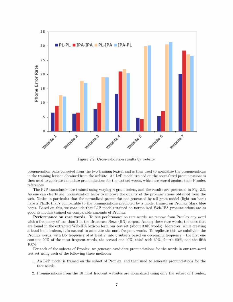
Figure 2.2: Cross-validation results by website.

pronunciation pairs collected from the two training lexica, and is then used to normalize the pronunciationsin the training lexicon obtained from the website. An L2P model trained on the normalized pronunciations isthen used to generate candidate pronunciations for the test set words, which are scored against their Pronlexreferences.

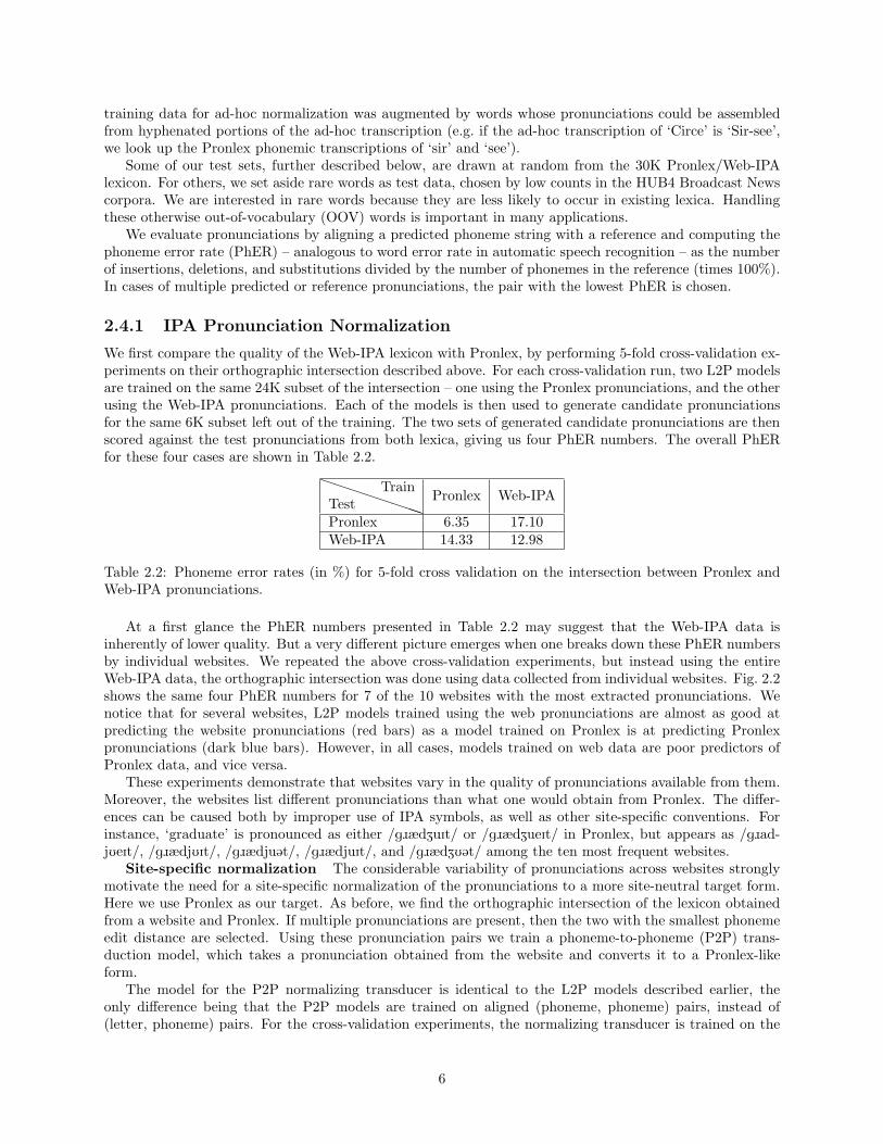
The P2P transducers are trained using varying n-gram orders, and the results are presented in Fig. 2.3.As one can clearly see, normalization helps to improve the quality of the pronunciations obtained from theweb. Notice in particular that the normalized pronunciations generated by a 5-gram model (light tan bars)have a PhER that’s comparable to the pronunciations predicted by a model trained on Pronlex (dark bluebars). Based on this, we conclude that L2P models trained on normalized Web-IPA pronunciations are asgood as models trained on comparable amounts of Pronlex.

Performance on rare words To test performance on rare words, we remove from Pronlex any wordwith a frequency of less than 2 in the Broadcast News (BN) corpus. Among these rare words, the ones thatare found in the extracted Web-IPA lexicon form our test set (about 3.8K words). Moreover, while creatinga hand-built lexicon, it is natural to annotate the most frequent words. To replicate this we subdivide thePronlex words, with BN frequency of at least 2, into 5 subsets based on decreasing frequency – the first onecontains 20% of the most frequent words, the second one 40%, third with 60%, fourth 80%, and the fifth100%.

For each of the subsets of Pronlex, we generate candidate pronunciations for the words in our rare-wordtest set using each of the following three methods:

1. An L2P model is trained on the subset of Pronlex, and then used to generate pronunciations for therare words.

2. Pronunciations from the 10 most frequent websites are normalized using only the subset of Pronlex,

7

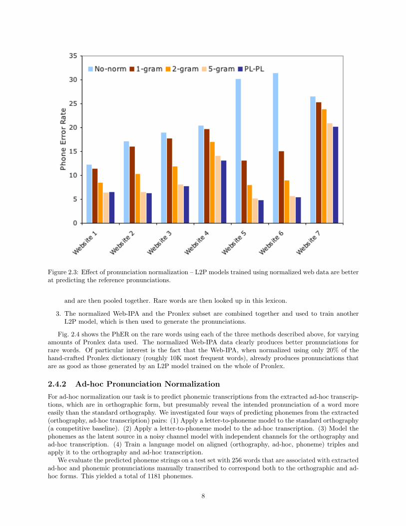
Figure 2.3: Effect of pronunciation normalization – L2P models trained using normalized web data are betterat predicting the reference pronunciations.

and are then pooled together. Rare words are then looked up in this lexicon.

3. The normalized Web-IPA and the Pronlex subset are combined together and used to train anotherL2P model, which is then used to generate the pronunciations.

Fig. 2.4 shows the PhER on the rare words using each of the three methods described above, for varyingamounts of Pronlex data used. The normalized Web-IPA data clearly produces better pronunciations forrare words. Of particular interest is the fact that the Web-IPA, when normalized using only 20% of thehand-crafted Pronlex dictionary (roughly 10K most frequent words), already produces pronunciations thatare as good as those generated by an L2P model trained on the whole of Pronlex.

2.4.2 Ad-hoc Pronunciation Normalization

For ad-hoc normalization our task is to predict phonemic transcriptions from the extracted ad-hoc transcrip-tions, which are in orthographic form, but presumably reveal the intended pronunciation of a word moreeasily than the standard orthography. We investigated four ways of predicting phonemes from the extracted(orthography, ad-hoc transcription) pairs: (1) Apply a letter-to-phoneme model to the standard orthography(a competitive baseline). (2) Apply a letter-to-phoneme model to the ad-hoc transcription. (3) Model thephonemes as the latent source in a noisy channel model with independent channels for the orthography andad-hoc transcription. (4) Train a language model on aligned (orthography, ad-hoc, phoneme) triples andapply it to the orthography and ad-hoc transcription.

We evaluate the predicted phoneme strings on a test set with 256 words that are associated with extractedad-hoc and phonemic pronunciations manually transcribed to correspond both to the orthographic and ad-hoc forms. This yielded a total of 1181 phonemes.

8

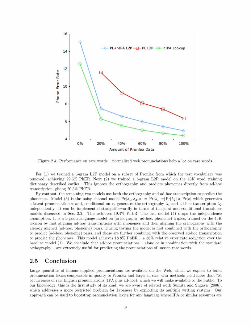
Figure 2.4: Performance on rare words – normalized web pronunciations help a lot on rare words.

For (1) we trained a 5-gram L2P model on a subset of Pronlex from which the test vocabulary wasremoved, achieving 29.5% PhER. Next (2) we trained a 5-gram L2P model on the 43K word trainingdictionary described earlier. This ignores the orthography and predicts phonemes directly from ad-hoctranscription, giving 20.5% PhER.

By contrast, the remaining two models use both the orthography and ad-hoc transcription to predict thephonemes. Model (3) is the noisy channel model Pr[λ1, λ2, π] = Pr[λ1 |π] Pr[λ2 |π] Pr[π] which generatesa latent pronunciation π and, conditional on π, generates the orthography λ1 and ad-hoc transcription λ2

independently. It can be implemented straightforwardly in terms of the joint and conditional transducermodels discussed in Sec. 2.2. This achieves 19.4% PhER. The last model (4) drops the independenceassumption. It is a 5-gram language model on (orthography, ad-hoc, phoneme) triples, trained on the 43Klexicon by first aligning ad-hoc transcriptions with phonemes and then aligning the orthography with thealready aligned (ad-hoc, phoneme) pairs. During testing the model is first combined with the orthographyto predict (ad-hoc, phoneme) pairs, and those are further combined with the observed ad-hoc transcriptionto predict the phonemes. This model achieves 18.8% PhER – a 36% relative error rate reduction over thebaseline model (1). We conclude that ad-hoc pronunciations – alone or in combination with the standardorthography – are extremely useful for predicting the pronunciations of unseen rare words.

2.5 Conclusion

Large quantities of human-supplied pronunciations are available on the Web, which we exploit to buildpronunciation lexica comparable in quality to Pronlex and larger in size. Our methods yield more than 7Moccurrences of raw English pronunciations (IPA plus ad-hoc), which we will make available to the public. Toour knowledge, this is the first study of its kind; we are aware of related work Sumita and Sugaya (2006),which addresses a more restricted problem for Japanese by exploiting its multiple writing systems. Ourapproach can be used to bootstrap pronunciation lexica for any language where IPA or similar resources are

9

available (preliminary work on French and German holds promise).One issue that we did not address is the usefulness of a pronunciation. For example, ad-hoc transcriptions

of common words often highlight unusual pronunciations (e.g. ‘cheenah’ for ‘China’, which is a Spanish firstname). This would be scored correct in Sec. 2.4.2, but there is a question of how many of these rarepronunciations we would want to put in our lexicon.

10

Chapter 3

Interscriptal Transcription

3.1 Introduction

A key problem in multilingual named entity recognition is recognition of the same name spelled in differentways in different scripts. For example, the (Polish) soccer player Maciej Zurawski’s name appears as마치에이주라브스키 in Korean, マチェイ・ジュラフスキ in Japanese, Мацей, Журавский in Russian, and ΜατσειΖουραφσκι in Greek, and 马西耶·茹拉夫斯基 in Chinese. All of these transcriptions share one thing incommon: they represent attempts to render, in the various scripts used by the languages in question, apronunciation that matches the original as closely as possible. The notion of match here can be quite loose,as it depends upon at least three factors:

• Knowledge of the original “correct” pronunciation of the name, which may be faulty.

• How well the name fits into the phonotactics of the target language.

• Possible language-specific strategies for spelling foreign names.

At the outset we wish to settle a terminological issue. The phenomenon we have just illustrated is mostcommonly referred to as transliteration in the literature. However, following Halpern (2007), we suggest thisusage is wrong. Properly construed, transliteration is a one-for-one — and hence unambiguously reversible— mapping between two symbol sets. Basically, true transliteration is a technical or scientific system forrepresenting one script in terms of another: one such system is Buckwalter’s system for transliterating ArabicBuckwalter (2002). What people typically call transliteration is really an instance of transcription. Tran-scription includes phonetic transcription, where a word is represented not in its standard orthography, butas a sequence of symbols in some alphabet (e.g., IPA, ArpaBet, WorldBet) that represents the pronunciationof the word; as well as what Halpern terms popular transcription, instances of which have been illustratedabove, where someone adopts a more or less regular system for representing a name in a foreign script inone’s own script.

Henceforth, we will adopt the term transcription, or popular transcription or interscriptal transcriptionif that term is unclear in context.

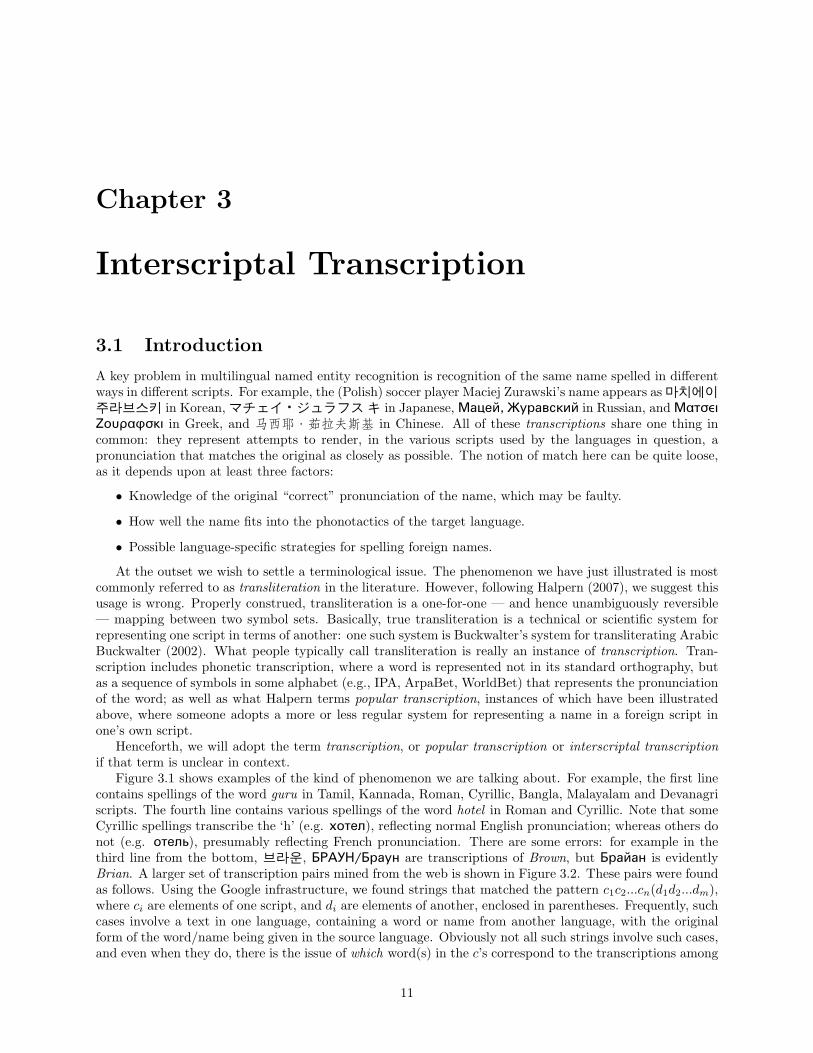
Figure 3.1 shows examples of the kind of phenomenon we are talking about. For example, the first linecontains spellings of the word guru in Tamil, Kannada, Roman, Cyrillic, Bangla, Malayalam and Devanagriscripts. The fourth line contains various spellings of the word hotel in Roman and Cyrillic. Note that someCyrillic spellings transcribe the ‘h’ (e.g. хотел), reflecting normal English pronunciation; whereas others donot (e.g. отель), presumably reflecting French pronunciation. There are some errors: for example in thethird line from the bottom, 브라운, БРАУН/Браун are transcriptions of Brown, but Брайан is evidentlyBrian. A larger set of transcription pairs mined from the web is shown in Figure 3.2. These pairs were foundas follows. Using the Google infrastructure, we found strings that matched the pattern c1c2...cn(d1d2...dm),where ci are elements of one script, and di are elements of another, enclosed in parentheses. Frequently, suchcases involve a text in one language, containing a word or name from another language, with the originalform of the word/name being given in the source language. Obviously not all such strings involve such cases,and even when they do, there is the issue of which word(s) in the c’s correspond to the transcriptions among

11

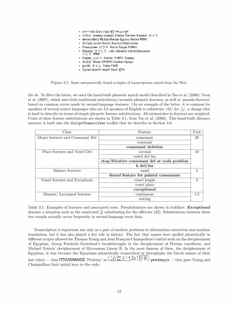
Figure 3.1: Some automatically found n-tuples of transcriptions mined from the Web.

the ds. To filter the latter, we used the hand-built phonetic match model described in Tao et al. (2006); Yoonet al. (2007), which uses both traditional articulatory/acoustic phonetic features, as well as ‘pseudo-features’based on common errors made by second-language learners. (As an example of the latter, it is common forspeakers of several source languages who are L2 speakers of English to substitute /dz/ for /j/, a change thatis hard to describe in terms of simple phonetic feature substitutions. All mismatches in features are weighted.Costs of these feature substitutions are shown in Table 3.1, from Tao et al. (2006). This hand-built distancemeasure is built into the ScriptTranscriber toolkit that we describe in Section 3.6.

Class Feature CostMajor features and Consonant Del consonant 20

sonorantconsonant deletion

Place features and Vowel Del coronal 10vowel del/ins

stop/fricative consonant del at coda positionh del/ins

Manner features nasal 5dorsal feature for palatal consonants

Vowel features and Exceptions vowel height 3vowel placeexceptional

Manner/ Laryngeal features continuous 1.5voicing

Table 3.1: Examples of features and associated costs. Pseudofeatures are shown in boldface. Exceptionaldenotes a situation such as the semivowel [j] substituting for the affricate [dZ]. Substitutions between thesetwo sounds actually occur frequently in second-language error data.

Transcription is important not only as a part of modern problems in information extraction and machinetranslation, but it has also played a key role in history. The fact that names were spelled phonetically indifferent scripts allowed for Thomas Young and Jean Francois Champollion’s initial work on the deciphermentof Egyptian, Georg Friedrich Grotefend’s breakthroughs in the decipherment of Persian cuneiform, andMichael Ventris’ decipherment of Mycenaean Linear B. In the most famous of these, the decipherment ofEgyptian, it was because the Egyptians phonetically transcribed in hieroglyphs the Greek names of their

last rulers — thus ΠΤΟΛΕΜΑΙΟΣ ‘Ptolemy’ as ptwlmyys — that gave Young andChampollion their initial keys to the code.

12

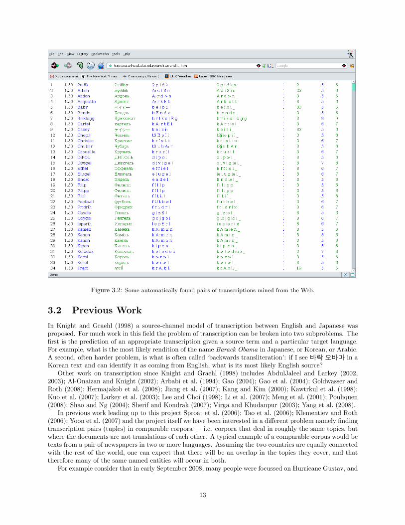
Figure 3.2: Some automatically found pairs of transcriptions mined from the Web.

3.2 Previous Work

In Knight and Graehl (1998) a source-channel model of transcription between English and Japanese wasproposed. For much work in this field the problem of transcription can be broken into two subproblems. Thefirst is the prediction of an appropriate transcription given a source term and a particular target language.For example, what is the most likely rendition of the name Barack Obama in Japanese, or Korean, or Arabic.A second, often harder problem, is what is often called ‘backwards transliteration’: if I see 바락오바마 in aKorean text and can identify it as coming from English, what is its most likely English source?

Other work on transcription since Knight and Graehl (1998) includes AbdulJaleel and Larkey (2002,2003); Al-Onaizan and Knight (2002); Arbabi et al. (1994); Gao (2004); Gao et al. (2004); Goldwasser andRoth (2008); Hermajakob et al. (2008); Jiang et al. (2007); Kang and Kim (2000); Kawtrkul et al. (1998);Kuo et al. (2007); Larkey et al. (2003); Lee and Choi (1998); Li et al. (2007); Meng et al. (2001); Pouliquen(2008); Shao and Ng (2004); Sherif and Kondrak (2007); Virga and Khudanpur (2003); Yang et al. (2008).

In previous work leading up to this project Sproat et al. (2006); Tao et al. (2006); Klementiev and Roth(2006); Yoon et al. (2007) and the project itself we have been interested in a different problem namely findingtranscription pairs (tuples) in comparable corpora — i.e. corpora that deal in roughly the same topics, butwhere the documents are not translations of each other. A typical example of a comparable corpus would betexts from a pair of newspapers in two or more languages. Assuming the two countries are equally connectedwith the rest of the world, one can expect that there will be an overlap in the topics they cover, and thattherefore many of the same named entities will occur in both.

For example consider that in early September 2008, many people were focussed on Hurricane Gustav, and

13

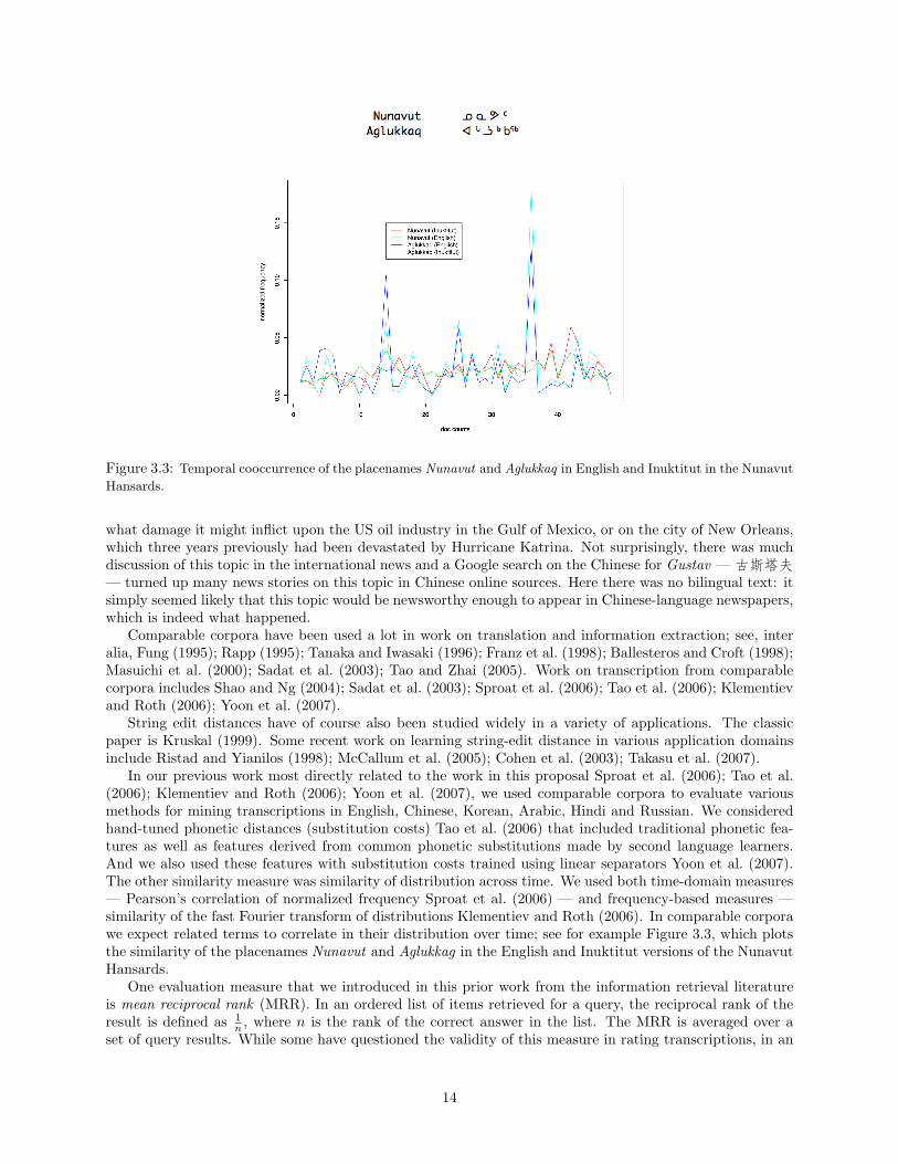
Figure 3.3: Temporal cooccurrence of the placenames Nunavut and Aglukkaq in English and Inuktitut in the Nunavut

Hansards.

what damage it might inflict upon the US oil industry in the Gulf of Mexico, or on the city of New Orleans,which three years previously had been devastated by Hurricane Katrina. Not surprisingly, there was muchdiscussion of this topic in the international news and a Google search on the Chinese for Gustav —古斯塔夫— turned up many news stories on this topic in Chinese online sources. Here there was no bilingual text: itsimply seemed likely that this topic would be newsworthy enough to appear in Chinese-language newspapers,which is indeed what happened.

Comparable corpora have been used a lot in work on translation and information extraction; see, interalia, Fung (1995); Rapp (1995); Tanaka and Iwasaki (1996); Franz et al. (1998); Ballesteros and Croft (1998);Masuichi et al. (2000); Sadat et al. (2003); Tao and Zhai (2005). Work on transcription from comparablecorpora includes Shao and Ng (2004); Sadat et al. (2003); Sproat et al. (2006); Tao et al. (2006); Klementievand Roth (2006); Yoon et al. (2007).

String edit distances have of course also been studied widely in a variety of applications. The classicpaper is Kruskal (1999). Some recent work on learning string-edit distance in various application domainsinclude Ristad and Yianilos (1998); McCallum et al. (2005); Cohen et al. (2003); Takasu et al. (2007).

In our previous work most directly related to the work in this proposal Sproat et al. (2006); Tao et al.(2006); Klementiev and Roth (2006); Yoon et al. (2007), we used comparable corpora to evaluate variousmethods for mining transcriptions in English, Chinese, Korean, Arabic, Hindi and Russian. We consideredhand-tuned phonetic distances (substitution costs) Tao et al. (2006) that included traditional phonetic fea-tures as well as features derived from common phonetic substitutions made by second language learners.And we also used these features with substitution costs trained using linear separators Yoon et al. (2007).The other similarity measure was similarity of distribution across time. We used both time-domain measures— Pearson’s correlation of normalized frequency Sproat et al. (2006) — and frequency-based measures —similarity of the fast Fourier transform of distributions Klementiev and Roth (2006). In comparable corporawe expect related terms to correlate in their distribution over time; see for example Figure 3.3, which plotsthe similarity of the placenames Nunavut and Aglukkag in the English and Inuktitut versions of the NunavutHansards.

One evaluation measure that we introduced in this prior work from the information retrieval literatureis mean reciprocal rank (MRR). In an ordered list of items retrieved for a query, the reciprocal rank of theresult is defined as 1

n , where n is the rank of the correct answer in the list. The MRR is averaged over aset of query results. While some have questioned the validity of this measure in rating transcriptions, in an

14

intended application where one has a given term in one language, and a list of candidate terms in the other,it is clear that the better the transcription system, the higher will be the rank of the correct candidate inthe list of possible matches.

Comparable corpora are, in fact, a good source of evidence for the hard job of backwards transliteration,described above. It is pretty hard on the basis of phonetic models alone to determine the correct originalspelling of a word transcribed into another script. But as Knight and Graehl’s original work discussed, alanguage model for the source language can narrow the targets considerably. Comparable corpora are asource of temporally appropriate language models. While in principle 古斯塔夫 in a contemporary Chinesenewspaper could come from a variety of original source names, in the current context it is unlikely to beanything besides Gustav.

3.3 Overview of deliverables

In light of the previous work that has been done on this problem the focus of this workshop was on betterunderstanding which features make the most sense for string comparison and for temporal cooccurrence.Specifically we will provide results that improve out understanding of which features to use for discriminativeraining of string comparison between transcriptions. We will discuss feature combination methods for string–and temporal cooccurrence.

To anticipate our results on string-comparison features: we show with data from Chinese that phoneticmatches can be better than orthographic matches, if you can predict the pronunciation with reasonableaccuracy. We also show that a very compact feature set – the hand-designed set of features from Yoon et al.(2007) works almost as well as feature sets containing hundreds or thousands of features derived by methodssimilar to those of Klementiev and Roth (2006). This suggests that linguistically derived features do have auseful place in transcription between scripts.

One of the stated goals of this workshop was to provide a set of open-source tools for mining transcriptionsfrom comparable corpora. We discuss our ScriptTranscriber toolkit in Section 3.6.

We note at the outset some of the data that we have been using in this project:

• Lexicons:

– Large (approx. 71,000 entry) English/Chinese name lexicon from the Linguistic Data Consortium(http://www.ldc.upenn.edu).

– 9,000 entry Korean/English lexicon from public source

– 1,750 entry Arabic/English lexicon from New Mexico State University

– Large transcription lexicon from multiple pairs of languages derived from the Web (>200K goodentries)

– 295K geographical names from the National Geospatial-Intelligence Agency (http://www1.nga.mil)

• Corpora, from the Linguistic Data Consortium, unless otherwise indicated:

– Chinese, English, Arabic gigaword

– ISI English/Chinese, English/Arabic found parallel corpora

– Less Commonly Taught Languages (LCTL) Thai/English corpus

– Nunavut Hansards (English/Inuktitut) (http://www.assembly.nu.ca/english/debates/index.html)

3.4 String Distances for Interscriptal Transcription

Graphical similarity can be used as an alternative metric to explicit phonetic features in judging the qualityof automatically extracted transcription pairs. The idea is that for most languages, graphical features often

15

correlate with phonetic features, from which transcriptions are typically derived. Klementiev and Roth Kle-mentiev and Roth (2006) applied a letter-based n-gram string comparison method to modeling transcriptionpairs between Russian and English. In their example, the English name Powell can be transcribed intoRussian as Pauel, where (ow, au) is an instance of letter-bigram pair features. A discriminative model canthen be trained to learn these pair features.

Although this approach obviates the process of hand crafting phonetic rules, and generally yields compet-ing results, it is not applicable in languages that have distinctive orthographies. The Chinese transcriptionfor Powell, for example, has only three characters: “鲍威尔”. The difference in length creates a problemfor effective alignment between these two scripts. Additionally, written Chinese is even less of a phoneticdescription of the language. Thus, a pair feature between English and Chinese does not really indicatephonetic correlation, making direct alignment seem awkward. Similar problems exist for English-Arabic andEnglish-Korean transcription models: in Arabic, vowels are omitted from the written script; in Hangul, thephonemic alphabet of Korean, “letters” are organized into characters that correspond to syllabic blocks. Inlanguage pairs where graphical features no longer correlate with phonetic features, a letter-based model likeabove will form incorrect correlations

The theme of our work then, is to find a way through which the methods of graphical comparison canbe applied to these three language pairs (i.e. English-Chinese, English-Arabic, and English-Korean). Weare particularly interested in looking for the best graphical features to use for each language pair. Sincetranscribed words tend to reflect the pronunciations of words in the language that they are transcribed from,we adopted the intuitive strategy of phonemic transformation on Arabic, Chinese and Korean. In doing so,the resulting phonemic transcriptions of Arabic, Chinese and Korean will better align with English letters.

Due to the availability of large amount of Chinese data, we focused on English-Chinese bi-directionaltranscription. In what follows, we describe the framework of our discriminative transcription model, followedby experimental feature selection in English-Chinese transcription and corresponding results. Extensibilityof our approach to other language pairs is discussed in the context of English-Arabic and English-Koreantranscriptions. Results show that using phonemic transcriptions of languages with non-alphabetic scripts isa generic solution to all three cases.

3.4.1 Framework

The entire framework of our discriminative model is described in this section. We set the discussion in thecontext of English-Chinese transcription for the ease of illustration.

3.4.1.1 Data

We based our work on three parallel dictionaries of named entities, among which the English-Chinese dictio-nary is the largest one with nearly 75,000 pairs of transcriptions. However, the original dictionary consistsof a number of Japaneses Kunyomi words. They are written in Chinese characters but are transcribed intoEnglish using Japanese pronunciations; therefore, there is no phonetic correlation between them at all. Wemanunally removed these Japanese Kunyomi names from the dictionary. The resulting dictionary contains71,548 entries. What remains after filtering is then partitioned into three parts: the first 90% of the dictio-nary used as the training set, the remaining part divided into 5% heldout and 5% testing parts (about 3,580examples each).

The other two dictionaries are considerably smaller in size. The English-Arabic dictionary has 1,750entries, while the English-Korean one has 9,046 entries.

3.4.1.2 Language Representation

We look for alternative representations of languages that can easily be aligned with each other, so thatit is possible to maximally exploit phonetic information from such graphical alignments. A representationcould plainly be the original script in which the language is written. Otherwise, phonemic transformation istypically used.

3.4.1.2.1 Representation of English For English, it is possible to construct a string-based languagemodel directly on its orthography. At the same time, there are plenty of pronunciation modeling toolkits for

16

converting English words to corresponding phonemes (at the model’s best guess). In our work, both repre-sentations are tested in combination with other languages. English phonemes are based on the pronunciationmodel of Festival.

3.4.1.2.2 Pinyin-based Phonemic Representation of Chinese Our initial approach was to takeChinese characters and convert them to Pinyin strings. Pinyin is a quasi-phonemic transcription systemused for describing the sounds of Chinese characters. Pinyin strings are written in regular English alphabet,although the pronunciation follows a rather unique set of rules. For example, the word huntington, transcribedto “亨廷顿” in Chinese, would be now represented in the Pinyin string heng ting dun (spaces bewteen Pinyinsyllables turned out to be a bad addition when corporated in discrinimative modeling). In the case ofhomophones, where a character may have multiple pronunciations, the most frequent Pinyin string is alwaysselected. This simple strategy actually makes sense: characters used in transcription should observe theirmost frequent pronunciation so that people are more likely to be able to pronounce the word.

Compared to characters, the Pinyin string of a Chinese word is more similar to the English counterpartin length. Pinyin also has the advantage of being an accurate and deterministic transformation scheme ofChinese characters. Given a character, it is always possible to map it onto the unique Pinyin string thatrepresents its pronunciation (given our frequencist assumption). However, Pinyin strings are biased to theparticular theory of Mandarin phonology that it is designed with, and therefore may ignore some phoneticdifferences that actually exist. For example, the fact that the three very different vowels in “si”, “shi” and“xi” are written with an “i” encodes the theory that at some level these are the same vowel, being influencedby the adjacent consonant. Other transcription systems, such as Wade-Giles, make different theoreticalclaims.

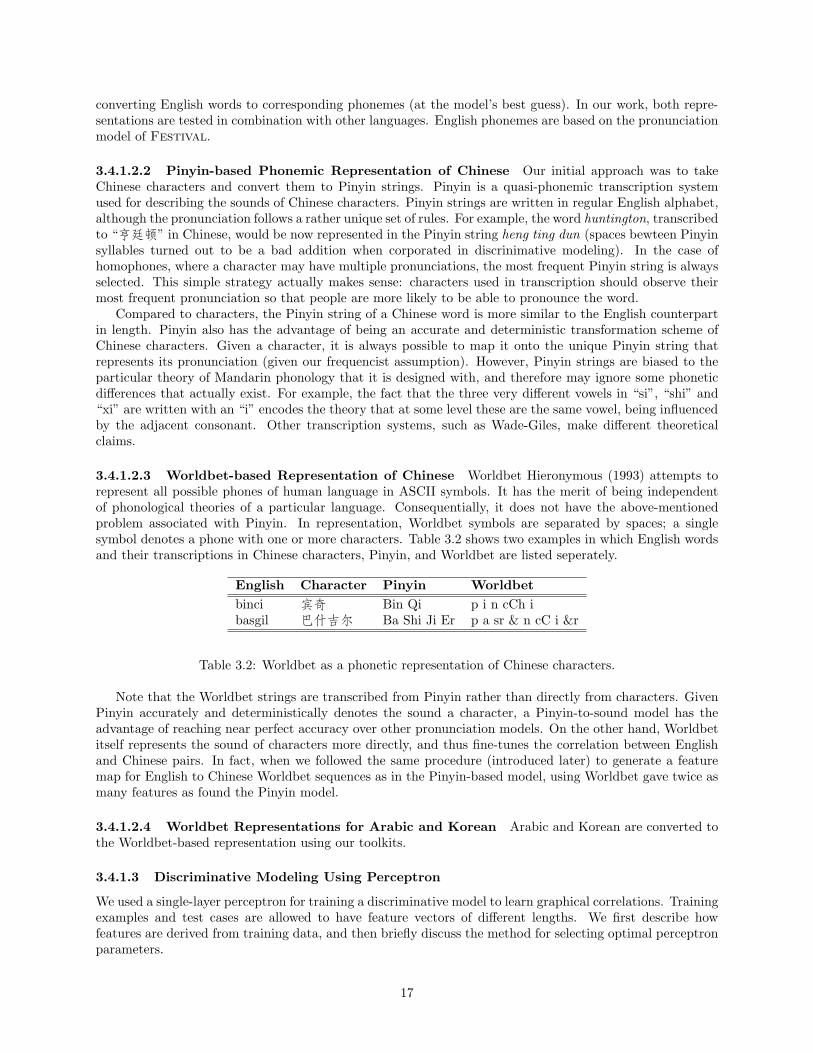
3.4.1.2.3 Worldbet-based Representation of Chinese Worldbet Hieronymous (1993) attempts torepresent all possible phones of human language in ASCII symbols. It has the merit of being independentof phonological theories of a particular language. Consequentially, it does not have the above-mentionedproblem associated with Pinyin. In representation, Worldbet symbols are separated by spaces; a singlesymbol denotes a phone with one or more characters. Table 3.2 shows two examples in which English wordsand their transcriptions in Chinese characters, Pinyin, and Worldbet are listed seperately.

English Character Pinyin Worldbetbinci 宾奇 Bin Qi p i n cCh ibasgil 巴什吉尔 Ba Shi Ji Er p a sr & n cC i &r

Table 3.2: Worldbet as a phonetic representation of Chinese characters.

Note that the Worldbet strings are transcribed from Pinyin rather than directly from characters. GivenPinyin accurately and deterministically denotes the sound a character, a Pinyin-to-sound model has theadvantage of reaching near perfect accuracy over other pronunciation models. On the other hand, Worldbetitself represents the sound of characters more directly, and thus fine-tunes the correlation between Englishand Chinese pairs. In fact, when we followed the same procedure (introduced later) to generate a featuremap for English to Chinese Worldbet sequences as in the Pinyin-based model, using Worldbet gave twice asmany features as found the Pinyin model.

3.4.1.2.4 Worldbet Representations for Arabic and Korean Arabic and Korean are converted tothe Worldbet-based representation using our toolkits.

3.4.1.3 Discriminative Modeling Using Perceptron

We used a single-layer perceptron for training a discriminative model to learn graphical correlations. Trainingexamples and test cases are allowed to have feature vectors of different lengths. We first describe howfeatures are derived from training data, and then briefly discuss the method for selecting optimal perceptronparameters.

17

3.4.1.3.1 Couplings of Bigram Substrings as Features Given a parallel dictionary of two languagesrepresented in appropriate forms, a set of letter-based bigram substrings are generated for each word in atranscription pair. Consider the previous example, where we have wE = huntington and wP = hengtingdun(Pinyin strings are concatenated together to resemble English orthography). Then, the sets of bigramsubstrings are:

wE ⇒< h, hu, . . . , on, n >

wP ⇒< h, he, . . . , un, n >

Underscores in here indicate either the beginning or the end of a word. Couplings of substrings from bothsets (such as, < hu, he >) are collected and used as training features of our model. We follow previous workwhere substrings that differ by one index position are paired Klementiev and Roth (2006). In addition tolocation-based restrictions, couplings that violate language-specific rules are also filtered out of the featurespace. For example, Chinese do not allow consonant clusters; therefore, a coupling like < nt, gt > offers arather improbable interscriptal relation and is not considered. Finally, low-frequency features are excludedfrom the feature space (current threshold is 1).

Each feature that remains in the feature space after filtration is then given a unique ID. We compiled thetraining part of dictionary entries into positive examples, and created four times as many negative examplesfrom positive ones with three different methods (see Experimental Results for details). Both categories ofexamples are represented in feature IDs for the perceptron to learn transcription patterns. Since there aremore negative examples than positive ones, any model trained on such data will be biased towards negativity.However, in corpus-based automatic extraction of transcription pairs, only one or two will be correct amongmany candidates. Therefore, the bias desirably works in our favor.

3.4.1.3.2 Parametric Optimization An iterative algorithm is applied to the training process to ensurethat the best possible parameters are selected for the discriminative model. We are particularly concernedwith two model parameters: feature cut-off value and the number of training iterations. The cut-off valuedetermines how frequent a feature must appear in the training data to be actually considered. The numberof iterations is most crucial because we want to prevent under-training as well as over-training.

In practice, we maintain an infinite training loop in which the values of these two parameters are increasedby 1 in each step. At the end of each cycle, the current model’s performance is tested on the heldout set (5%of the dictionary size). That is, we monitor the performance of the model with respect to heldout data. Ifits performance stops improving for 3 consecutive cycles, we cease this iterative training process and reporta set of optimal parameters. The detailed procedure is as follows:

• Set the model to run at cut-off values from 1 to 5 on the training data;

• For each feature cut-off value, train the model with 1 iteration;

• Increment the number of training iterations by one, retrain the model, and monitor the testing resultson heldout data for the most recent three models;

• Repeat the above step; if the model stops improving by at least 0.04% in the 3-session interval, ceasetraining, and report the first one of the most recent three models as the best one for current cut-off.

This iterative training process selects optimal values of cut-off and iteration number for a given trainingtask in an ad-hot fashion. We then use the particular model trained with optimal parameters in subsequenttesting phases.

3.4.2 Experimental Results

Experimental results are reported in this section. Binary classification was carried out on the test data(5% of the dictionary) with models trained as described. Two classes of test cases are present in the testdata: plausible transcription pairs (positive) and implausible ones (negative). These negative test cases aregenerated from positive ones as in training examples. We are primarily interested in finding how accuratelythe trained model can distinguish between these two kinds.

18

3.4.2.1 Accuracy of Models for English-Chinese Transcription

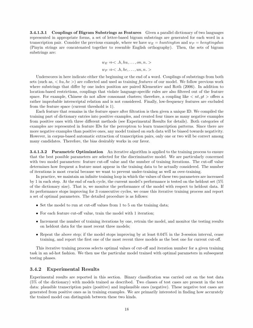
We experimented with three different models: the first one uses English letters and Chinese Pinyin strings(EL-CP); the second one uses English letters and Chinese phonemic transcription based on Worldbet (EL-CW); the third one uses English Phonemes produced by Festival instead of plain letters, but keeps theChinese phonemic transcription in Worldbet (EP-CW). Additionally, we compared these models with amodel based-on handcrafted phonetic features in the work of Yoon et al. (2007). With nearly 65,000 positivetraining examples and four times as many negative examples, these models all performed very well on thesimilarly proportioned test data. Table 3.3 shows the accuracy figures.

Positive Negative OverallPhonetic 88.5% 97.0% 95.5%EL-CP 92.3% 98.1% 96.3%EL-CW 97.7% 99.6% 99.4%EP-CW 95.9% 99.1% 98.5%Baseline – – 80.0%

Table 3.3: Model accuracy on positive and negative test cases, and its overall performance, compared to themodel based on phonetic features as well as the baseline (a blind model).

All three models are more likely to correctly identify that a test case is an implausible transcription pair,than to identify it as plausible. This is not surprising, because, as we have stated, the ratio between thenumber of negative examples and that of positive ones is 4 to 1. Consequently, if a model were to classifyevery cases presented as negative, it would achieve a baseline accuracy of 80%. Fortunately, even the worsemodel above (English letters to Chinese Pinyin letters) still outperforms the baseline signficantly by 16.3%.

Note that the best model in Table 3.3 is the English letters to Chinese Worldbet model. We think thisis due to two obvious reasons. First, Worldbet, as discussed above, represents Mandarin pronunciation in away that is unbiased by any phonological theories. Therefore, it is more faithful in capturing the phoneticproperties of Mandarin words than Pinyin. Second, Englis letters are also better than phonemes becausethe latter may contain errors due to the pronunciation toolkit that we use. These noises debilitated theperformance of the English phoneme to Chinese Worldbet model.

These data also indicate that discriminative training using perceptron is an effective method in the contextof identifying English-Chinese transcription pairs. Compared to the method based on phonetic rules, it hasa clear advantage due to a much larger set of available features. We show this method can be extend tobuilding English-Arabic and English-Korean models in the next section.

3.4.2.2 Effect of Training Size

The above performance was reported from models with more than 300,000 examples in training data (includ-ing both positive and negative ones). To understand whether it is possible to achieve comparable performancewith smaller training sets, we randomly sampled eight subsets from the training data, ranging from 500 to250,000 examples. Trained models were tested on the same test data as used previously.

We evaluated the models for their accuracy on binary classification of positive and negative test casesusing f-scores as in Formula 3.1.

F =2 × (precision × recall)

precision + recall(3.1)

That is, we evaluated the task of classifying test cases as if it were two information retrieval tasks. Inone, the perceptron model tries to retrieve as many positive examples as possible (recall), while controlingfor the number of false alarms (precision) at the same time. In the other, it tries to do the same thing withnegative examples. But these two tasks are dependent since the classification targets are binary.

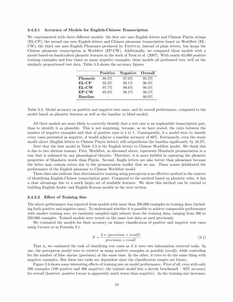
Figure 3.4 shows some interesting effects of training size on model performance. First of all, even with only500 examples (100 positive and 400 negative), the trained model hits a decent benchmark – 92% accuracyfor overall (however, positive f-score is apparently much worse than negative). As the training size increases,

19

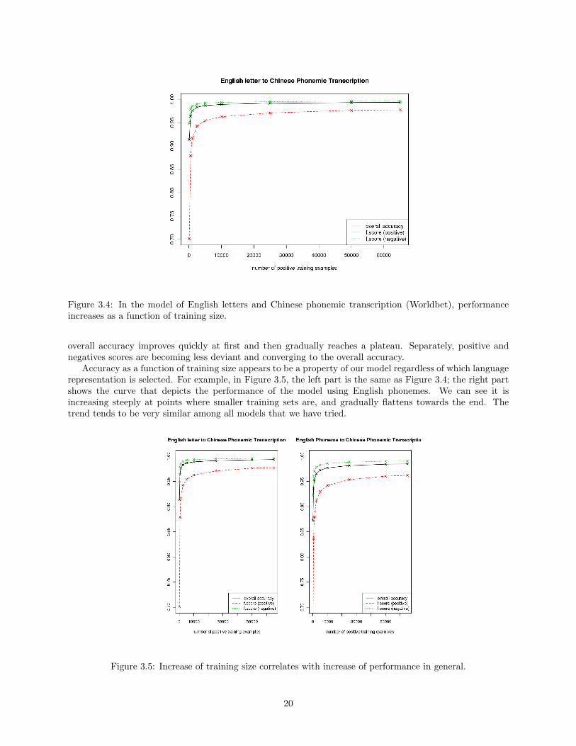
Figure 3.4: In the model of English letters and Chinese phonemic transcription (Worldbet), performanceincreases as a function of training size.

overall accuracy improves quickly at first and then gradually reaches a plateau. Separately, positive andnegatives scores are becoming less deviant and converging to the overall accuracy.

Accuracy as a function of training size appears to be a property of our model regardless of which languagerepresentation is selected. For example, in Figure 3.5, the left part is the same as Figure 3.4; the right partshows the curve that depicts the performance of the model using English phonemes. We can see it isincreasing steeply at points where smaller training sets are, and gradually flattens towards the end. Thetrend tends to be very similar among all models that we have tried.

Figure 3.5: Increase of training size correlates with increase of performance in general.

20

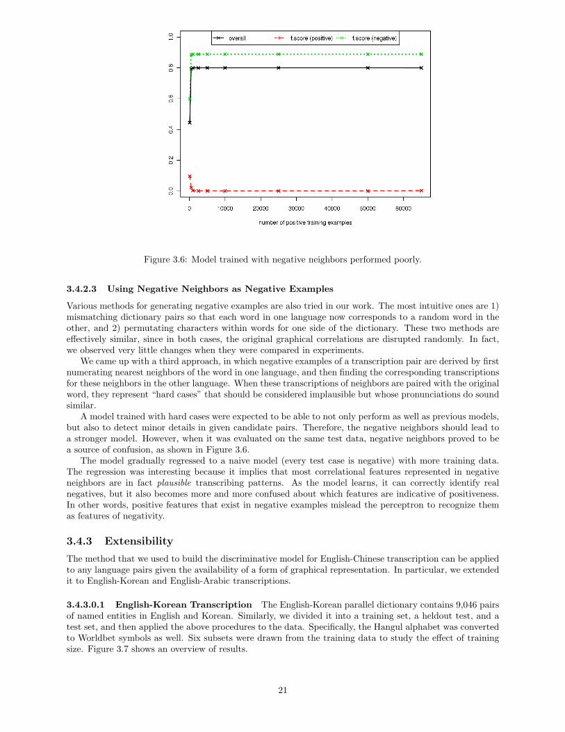
Figure 3.6: Model trained with negative neighbors performed poorly.

3.4.2.3 Using Negative Neighbors as Negative Examples

Various methods for generating negative examples are also tried in our work. The most intuitive ones are 1)mismatching dictionary pairs so that each word in one language now corresponds to a random word in theother, and 2) permutating characters within words for one side of the dictionary. These two methods areeffectively similar, since in both cases, the original graphical correlations are disrupted randomly. In fact,we observed very little changes when they were compared in experiments.

We came up with a third approach, in which negative examples of a transcription pair are derived by firstnumerating nearest neighbors of the word in one language, and then finding the corresponding transcriptionsfor these neighbors in the other language. When these transcriptions of neighbors are paired with the originalword, they represent “hard cases” that should be considered implausible but whose pronunciations do soundsimilar.

A model trained with hard cases were expected to be able to not only perform as well as previous models,but also to detect minor details in given candidate pairs. Therefore, the negative neighbors should lead toa stronger model. However, when it was evaluated on the same test data, negative neighbors proved to bea source of confusion, as shown in Figure 3.6.

The model gradually regressed to a naive model (every test case is negative) with more training data.The regression was interesting because it implies that most correlational features represented in negativeneighbors are in fact plausible transcribing patterns. As the model learns, it can correctly identify realnegatives, but it also becomes more and more confused about which features are indicative of positiveness.In other words, positive features that exist in negative examples mislead the perceptron to recognize themas features of negativity.

3.4.3 Extensibility

The method that we used to build the discriminative model for English-Chinese transcription can be appliedto any language pairs given the availability of a form of graphical representation. In particular, we extendedit to English-Korean and English-Arabic transcriptions.

3.4.3.0.1 English-Korean Transcription The English-Korean parallel dictionary contains 9,046 pairsof named entities in English and Korean. Similarly, we divided it into a training set, a heldout test, and atest set, and then applied the above procedures to the data. Specifically, the Hangul alphabet was convertedto Worldbet symbols as well. Six subsets were drawn from the training data to study the effect of trainingsize. Figure 3.7 shows an overview of results.

21

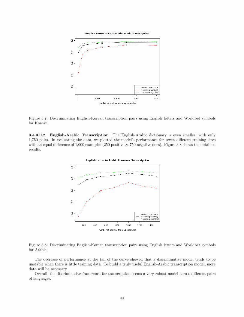
Figure 3.7: Discriminating English-Korean transcription pairs using English letters and Worldbet symbolsfor Korean.

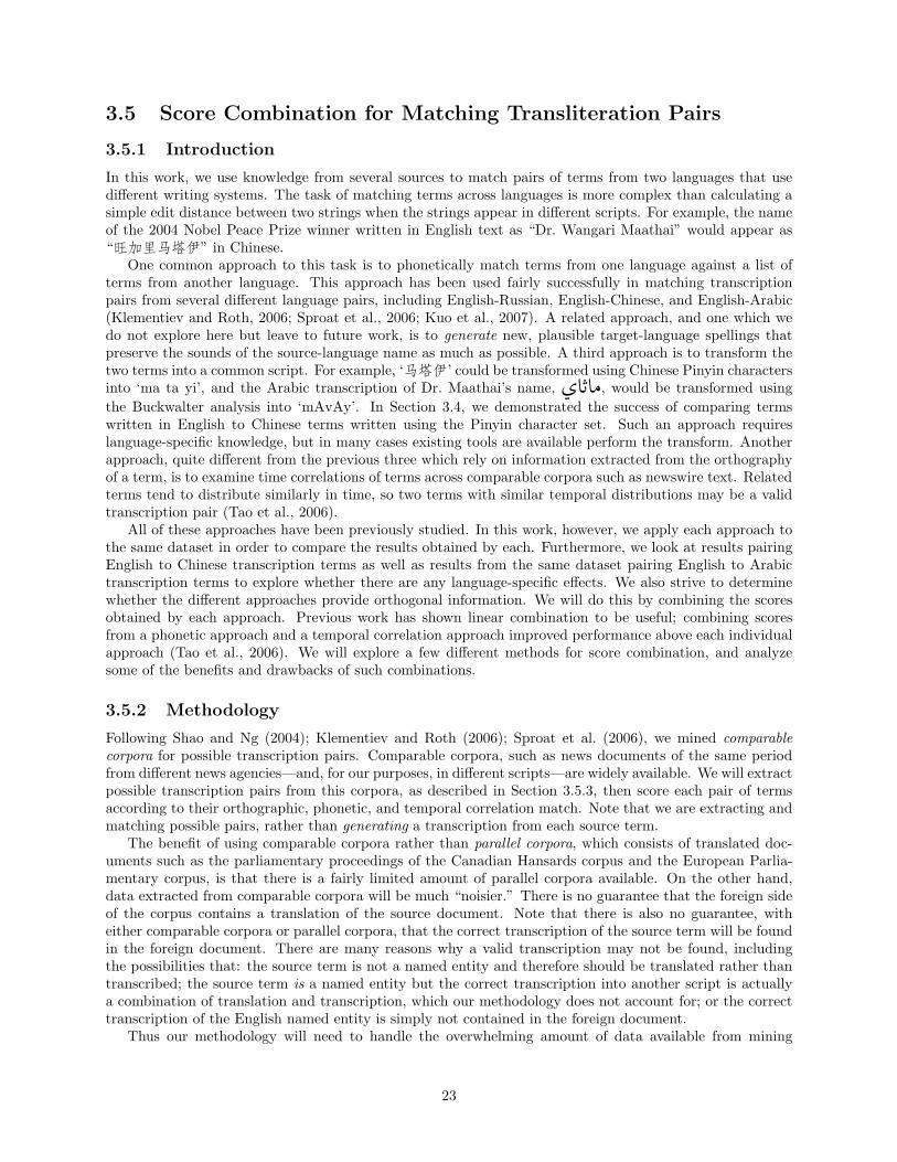
3.4.3.0.2 English-Arabic Transcription The English-Arabic dictionary is even smaller, with only1,750 pairs. In evaluating the data, we plotted the model’s performance for seven different training sizeswith an equal difference of 1,000 examples (250 positive & 750 negative ones). Figure 3.8 shows the obtainedresults.

Figure 3.8: Discriminating English-Korean transcription pairs using English letters and Worldbet symbolsfor Arabic.

The decrease of performance at the tail of the curve showed that a discriminative model tends to beunstable when there is little training data. To build a truly useful English-Arabic transcription model, moredata will be necessary.

Overall, the discriminative framework for transcription seems a very robust model across different pairsof languages.

22

3.5 Score Combination for Matching Transliteration Pairs

3.5.1 Introduction

In this work, we use knowledge from several sources to match pairs of terms from two languages that usedifferent writing systems. The task of matching terms across languages is more complex than calculating asimple edit distance between two strings when the strings appear in different scripts. For example, the nameof the 2004 Nobel Peace Prize winner written in English text as “Dr. Wangari Maathai” would appear as“旺加里马塔伊” in Chinese.

One common approach to this task is to phonetically match terms from one language against a list ofterms from another language. This approach has been used fairly successfully in matching transcriptionpairs from several different language pairs, including English-Russian, English-Chinese, and English-Arabic(Klementiev and Roth, 2006; Sproat et al., 2006; Kuo et al., 2007). A related approach, and one which wedo not explore here but leave to future work, is to generate new, plausible target-language spellings thatpreserve the sounds of the source-language name as much as possible. A third approach is to transform thetwo terms into a common script. For example, ‘马塔伊’ could be transformed using Chinese Pinyin charactersinto ‘ma ta yi’, and the Arabic transcription of Dr. Maathai’s name, ي , would be transformed usingthe Buckwalter analysis into ‘mAvAy’. In Section 3.4, we demonstrated the success of comparing termswritten in English to Chinese terms written using the Pinyin character set. Such an approach requireslanguage-specific knowledge, but in many cases existing tools are available perform the transform. Anotherapproach, quite different from the previous three which rely on information extracted from the orthographyof a term, is to examine time correlations of terms across comparable corpora such as newswire text. Relatedterms tend to distribute similarly in time, so two terms with similar temporal distributions may be a validtranscription pair (Tao et al., 2006).

All of these approaches have been previously studied. In this work, however, we apply each approach tothe same dataset in order to compare the results obtained by each. Furthermore, we look at results pairingEnglish to Chinese transcription terms as well as results from the same dataset pairing English to Arabictranscription terms to explore whether there are any language-specific effects. We also strive to determinewhether the different approaches provide orthogonal information. We will do this by combining the scoresobtained by each approach. Previous work has shown linear combination to be useful; combining scoresfrom a phonetic approach and a temporal correlation approach improved performance above each individualapproach (Tao et al., 2006). We will explore a few different methods for score combination, and analyzesome of the benefits and drawbacks of such combinations.

3.5.2 Methodology

Following Shao and Ng (2004); Klementiev and Roth (2006); Sproat et al. (2006), we mined comparablecorpora for possible transcription pairs. Comparable corpora, such as news documents of the same periodfrom different news agencies—and, for our purposes, in different scripts—are widely available. We will extractpossible transcription pairs from this corpora, as described in Section 3.5.3, then score each pair of termsaccording to their orthographic, phonetic, and temporal correlation match. Note that we are extracting andmatching possible pairs, rather than generating a transcription from each source term.

The benefit of using comparable corpora rather than parallel corpora, which consists of translated doc-uments such as the parliamentary proceedings of the Canadian Hansards corpus and the European Parlia-mentary corpus, is that there is a fairly limited amount of parallel corpora available. On the other hand,data extracted from comparable corpora will be much “noisier.” There is no guarantee that the foreign sideof the corpus contains a translation of the source document. Note that there is also no guarantee, witheither comparable corpora or parallel corpora, that the correct transcription of the source term will be foundin the foreign document. There are many reasons why a valid transcription may not be found, includingthe possibilities that: the source term is not a named entity and therefore should be translated rather thantranscribed; the source term is a named entity but the correct transcription into another script is actuallya combination of translation and transcription, which our methodology does not account for; or the correcttranscription of the English named entity is simply not contained in the foreign document.

Thus our methodology will need to handle the overwhelming amount of data available from mining

23

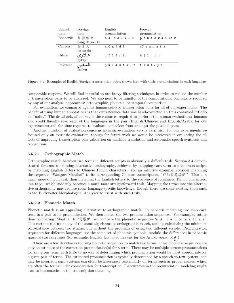
English Foreign English Foreignterm term pronunciation pronunciation

Bondevik 邦德维克 b A: n d I v I k p a N t & w & i kh &

bang de wei ke

Canada 加拿大 k @ n & d & cC y a n a t a

jia na da

Hilary ري h I l & r i: h j l j r j

hyl’ry

Palestine p @ l & s t a I n f l s t∼ j n

flsTyn

Figure 3.9: Examples of English/foreign transcription pairs, shown here with their pronunciations in each language.

comparable corpora. We will find it useful to use heavy filtering techniques in order to reduce the numberof transcription pairs to be analyzed. We also need to be mindful of the computational complexity requiredby any of our analysis approaches: orthographic, phonetic, or temporal comparison.

For evaluation, we compared against human-selected transcription pairs for all of our experiments. Thebenefit of using human annotations is that our reference data was hand-corrected an thus contained little tono “noise.” The drawback, of course, is the resources required to perform the human evaluations: humanswho could fluently read each of the languages in the pair (English/Chinese and English/Arabic for ourexperiments) and the time required to evaluate and select from amongst the possible pairs.

Another question of evaluation concerns intrinsic evaluation versus extrinsic. For our experiments wefocused only on extrinsic evaluation, though for future work we would be interested in evaluating the ef-fects of improving transcription pair validation on machine translation and automatic speech synthesis andrecognition.

3.5.2.1 Orthographic Match

Orthographic match between two terms in different scripts is obviously a difficult task. Section 3.4 demon-strated the success of using alternative orthography, achieved by mapping each term to a common script,by matching English letters to Chinese Pinyin characters. For an intuitive example, consider matchingthe sequence “Wangari Maathai” to its corresponding Chinese transcription, “旺加里马塔伊.” This is amuch more difficult task than matching the English letters to the sequence of romanized Pinyin characters,‘ma ta yi,’ which suddenly becomes a much more straightforward task. Mapping the terms into the alterna-tive orthography may require some language-specific knowledge, though there are some existing tools suchas the Buckwalter Morphological Analyzer to assist with such tasks.

3.5.2.2 Phonetic Match

Phonetic match is an appealing alternative to orthographic match. In phonetic matching, we map eachterm in a pair to its pronunciation. We then match the two pronunciation sequences. For example, ratherthan comparing ‘Maathai’ to ‘马塔伊’, we compare the phonetic sequences ‘m A: t a I’ to ‘m a th a i’.This method can use many of the same algorithms as orthographic match, such as calculating the minimumedit-distance between two strings, but without the problems of using two different scripts. Pronunciationsequences for different languages use the same set of phonetic symbols, modulo the differences in phoneticspace of two languages (for example, English has no equivalent for the Arabic sound of .(ع

There are a few drawbacks to using phonetic sequences to match two terms. First, phonetic sequences areonly an estimate of the correction pronunciation(s) for a term. There may be multiple correct pronunciationsfor any given term, with little to no way of determining which pronunciation would be most appropriate fora given pair of terms. The estimated pronunciation is typically determined by a speech-to-text system, andmay be incorrect; such systems can often be inaccurate particularly on terms such as proper names, whichare often the terms under consideration for transcription. Inaccuracies in the pronunciation modeling mightlead to inaccuracies in the transcription matching.

24

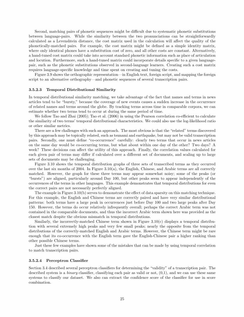
Second, matching pairs of phonetic sequences might be difficult due to systematic phonetic substitutionsbetween language-pairs. While the similarity between the two pronunciations can be straightforwardlycalculated as a Levenshtein distance, the cost matrix used in the calculation will affect the quality of thephonetically-matched pairs. For example, the cost matrix might be defined as a simple identity matrix,where only identical phones have a substitution cost of zero, and all other costs are constant. Alternatively,a hand-tuned cost matrix could take into account standard phonetic information such as place of articulationand locution. Furthermore, such a hand-tuned matrix could incorporate details specific to a given language-pair, such as the phonetic substitutions observed in second-language learners. Creating such a cost matrixrequires language-specific knowledge and time spent on creating and tuning the costs.

Figure 3.9 shows the orthographic representation—in English text, foreign script, and mapping the foreignscript to an alternative orthography—and phonetic sequences of several transcription pairs.

3.5.2.3 Temporal Distributional Similarity

In temporal distributional similarity matching, we take advantage of the fact that names and terms in newsarticles tend to be “bursty,” because the coverage of new events causes a sudden increase in the occurrenceof related names and terms around the globe. By tracking terms across time in comparable corpora, we canestimate whether two terms tend to occur at during the same period of time.

We follow Tao and Zhai (2005); Tao et al. (2006) in using the Pearson correlation co-efficient to calculatethe similarity of two terms’ temporal distributional characteristics. We could also use the log-likelihood ratioor other similar metrics.

There are a few challenges with such an approach. The most obvious is that the “related” terms discoveredby this approach may be topically related, such as tsunami and earthquake, but may not be valid transcriptionpairs. Secondly, one must define “co-occurrence” carefully: clearly two terms that occur in news articleson the same day would be co-occurring terms, but what about within one day of the other? Two days? Aweek? These decisions can affect the utility of this approach. Finally, the correlation values calculated foreach given pair of terms may differ if calculated over a different set of documents, and scaling up to largesets of documents may be challenging.

Figure 3.10 shows the temporal distribution graphs of three sets of transcribed terms as they occurredover the last six months of 2004. In Figure 3.10(a), the English, Chinese, and Arabic terms are all correctlymatched. However, the graph for these three terms may appear somewhat noisy; some of the peaks (or“bursts”) are aligned, particularly around Day 100, but other peaks seem to appear independently of theoccurrences of the terms in other languages. This example demonstrates that temporal distributions for eventhe correct pairs are not necessarily perfectly aligned.

The example in Figure 3.10(b) serves to demonstrate the effect of data sparsity on this matching technique.For this example, the English and Chinese terms are correctly paired and have very similar distributionalpatterns: both terms have a large peak in occurrences just before Day 100 and two large peaks after Day150. However, the terms do occur relatively infrequently overall; perhaps the correct Arabic term was notcontained in the comparable documents, and thus the incorrect Arabic term shown here was provided as theclosest match despite the obvious mismatch in temporal distributions.

Similarly, the incorrectly-matched Chinese term shown in Figure 3.10(c) displays a temporal distribu-tion with several extremely high peaks and very few small peaks; nearly the opposite from the temporaldistributions of the correctly-matched English and Arabic terms. However, the Chinese term might be rareenough that its co-occurrence with the English term gave the English-Chinese pair a higher ranking thanother possible Chinese terms.

Just these few examples have shown some of the mistakes that can be made by using temporal correlationto match transcription pairs.

3.5.2.4 Perceptron Classifier

Section 3.4 described several perceptron classifiers for determining the “validity” of a transcription pair. Thedescribed system is a binary classifier, classifying each pair as valid or not, (0,1), and we can use these samesystems to classify our dataset. We also can extract the confidence score of the classifier for use in scorecombination.

25

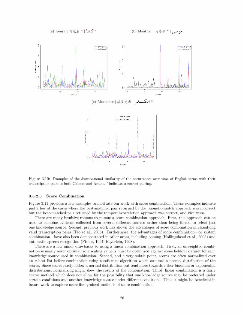
(a) Kenya | 肯尼亚 * | * (b) Maathai | 马塔伊 * |

(c) Alexander | 埃里克森 | ر ا *

Figure 3.10: Examples of the distributional similarity of the occurrences over time of English terms with their

transcription pairs in both Chinese and Arabic. ∗Indicates a correct pairing.

3.5.2.5 Score Combination

Figure 3.11 provides a few examples to motivate our work with score combination. These examples indicatejust a few of the cases where the best-matched pair returned by the phonetic-match approach was incorrectbut the best-matched pair returned by the temporal-correlation approach was correct, and vice versa.

There are many intuitive reasons to pursue a score combination approach. First, this approach can beused to combine evidence collected from several different sources rather than being forced to select justone knowledge source. Second, previous work has shown the advantages of score combination in classifyingvalid transcription pairs (Tao et al., 2006). Furthermore, the advantages of score combination—or systemcombination—have also been demonstrated in other areas, including parsing (Hollingshead et al., 2005) andautomatic speech recognition (Fiscus, 1997; Beyerlein, 1998).

There are a few minor drawbacks to using a linear combination approach. First, an unweighted combi-nation is nearly never optimal, so a scaling value α must be optimized against some heldout dataset for eachknowledge source used in combination. Second, and a very subtle point, scores are often normalized overan n-best list before combination using a soft-max algorithm which assumes a normal distribution of thescores. Since scores rarely follow a normal distribution but tend more towards either binomial or exponentialdistributions, normalizing might skew the results of the combination. Third, linear combination is a fairlycoarse method which does not allow for the possibility that one knowledge source may be preferred undercertain conditions and another knowledge source under different conditions. Thus it might be beneficial infuture work to explore more fine-grained methods of score combination.

26

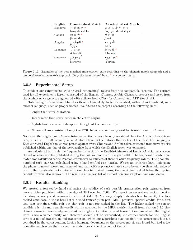
English Phonetic-best Match Correlation-best Match

Bondevik 邦德维克 * 波及印度尼西亚bang de wei ke bo ji yin du ni xi ya

Canada 加拿大 * 及内地jia na da ji nei di

Angeles ا * را ا’njlys ’ldr’sh

Lebanese 日本地 黎巴嫩 *ri ben di li ba nen

Gazprom وم ز *

kyswfym j’zbrwm

Figure 3.11: Examples of the best-matched transcription pairs according to the phonetic-match approach and a

temporal correlation–match approach. Only the term marked by an ∗ is a correct match.

3.5.3 Experimental Setup

To conduct our experiments, we extracted “interesting” tokens from the comparable corpora. The corporaused for all experiments herein consisted of the English, Chinese, Arabic Gigaword corpora and news fromthe Xinhua news agency, augmented with articles from CNA (for Chinese) and AFP (for Arabic).

“Interesting” tokens were defined as those tokens likely to be transcribed, rather than translated, intoanother language, such as proper names. We filtered the corpora according to the following rules:

– Longer than three characters

– Occurs more than seven times in the entire corpus

– English tokens were initial-capped throughout the entire corpus

– Chinese tokens consisted of only the 1250 characters commonly used for transcription in Chinese

Note that the English and Chinese token extraction is more heavily restricted than the Arabic token extrac-tion, which will result in many more Arabic tokens in the dataset than either of the other two languages.Each extracted English token was paired against every Chinese and Arabic token extracted from news articlespublished within one day of the news article from which the English token was extracted.

We calculated term relative frequencies for each of the English-Chinese and English-Arabic pairs acrossthe set of news articles published during the last six months of the year 2004. The temporal distribution–match was calculated as the Pearson correlation co-efficient of these relative frequency values. The phonetic-match of each pair was calculated using a hand-crafted cost matrix. We set an arbitrary hard-limit usingthe phonetic-match score, and removed any pair with a phonetic-match score below the threshold value often. If the thresholded set contained more than ten paired terms, then anything ranked below the top tencandidates were also removed. The result is an n-best list of at most ten transcription-pair candidates.

3.5.4 Results: Ranking

We created a test-set by hand-evaluating the validity of each possible transcription pair extracted fromnews articles published within one day of 30 December 2004. We report on several evaluation metrics,including accuracy and mean-reciprocal rank (MRR). Accuracy simply indicates how frequently the top-ranked candidate in the n-best list is a valid transcription pair. MRR provides “partial-credit” for n-bestlists that contain a valid pair but that pair is not top-ranked in the list. The higher-ranked the correctcandidate is, the more partial-credit will be awarded by the MRR metric. Recall from Section 3.5.2 thatthere are several reasons why an n-best list might not contain a valid transcription pair at all: the Englishterm is not a named entity and therefore should not be transcribed; the correct match for the Englishterm is a mix of translation and transcription, which our algorithms may not find; the correct match is notcontained in the corresponding foreign-language document; or the correct match was found but had a lowphonetic-match score that pushed the match below the threshold of the list.

27

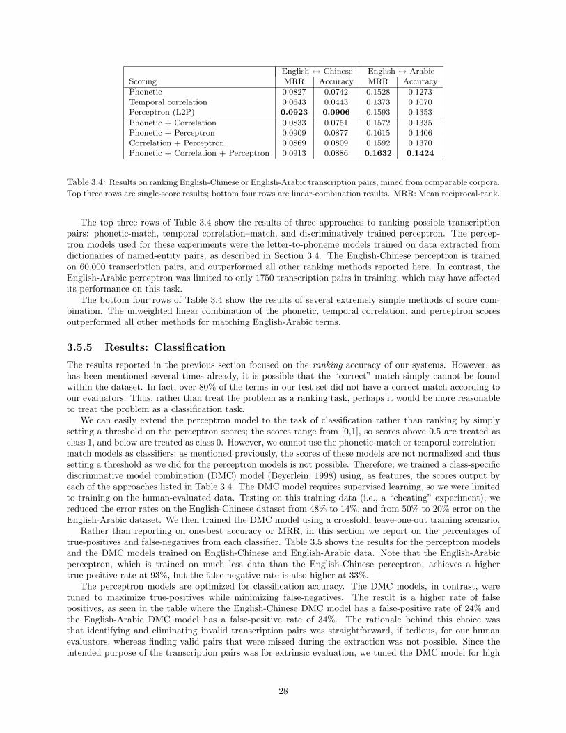
English ↔ Chinese English ↔ ArabicScoring MRR Accuracy MRR Accuracy

Phonetic 0.0827 0.0742 0.1528 0.1273Temporal correlation 0.0643 0.0443 0.1373 0.1070Perceptron (L2P) 0.0923 0.0906 0.1593 0.1353

Phonetic + Correlation 0.0833 0.0751 0.1572 0.1335Phonetic + Perceptron 0.0909 0.0877 0.1615 0.1406Correlation + Perceptron 0.0869 0.0809 0.1592 0.1370Phonetic + Correlation + Perceptron 0.0913 0.0886 0.1632 0.1424

Table 3.4: Results on ranking English-Chinese or English-Arabic transcription pairs, mined from comparable corpora.

Top three rows are single-score results; bottom four rows are linear-combination results. MRR: Mean reciprocal-rank.

The top three rows of Table 3.4 show the results of three approaches to ranking possible transcriptionpairs: phonetic-match, temporal correlation–match, and discriminatively trained perceptron. The percep-tron models used for these experiments were the letter-to-phoneme models trained on data extracted fromdictionaries of named-entity pairs, as described in Section 3.4. The English-Chinese perceptron is trainedon 60,000 transcription pairs, and outperformed all other ranking methods reported here. In contrast, theEnglish-Arabic perceptron was limited to only 1750 transcription pairs in training, which may have affectedits performance on this task.

The bottom four rows of Table 3.4 show the results of several extremely simple methods of score com-bination. The unweighted linear combination of the phonetic, temporal correlation, and perceptron scoresoutperformed all other methods for matching English-Arabic terms.

3.5.5 Results: Classification

The results reported in the previous section focused on the ranking accuracy of our systems. However, ashas been mentioned several times already, it is possible that the “correct” match simply cannot be foundwithin the dataset. In fact, over 80% of the terms in our test set did not have a correct match according toour evaluators. Thus, rather than treat the problem as a ranking task, perhaps it would be more reasonableto treat the problem as a classification task.

We can easily extend the perceptron model to the task of classification rather than ranking by simplysetting a threshold on the perceptron scores; the scores range from [0,1], so scores above 0.5 are treated asclass 1, and below are treated as class 0. However, we cannot use the phonetic-match or temporal correlation–match models as classifiers; as mentioned previously, the scores of these models are not normalized and thussetting a threshold as we did for the perceptron models is not possible. Therefore, we trained a class-specificdiscriminative model combination (DMC) model (Beyerlein, 1998) using, as features, the scores output byeach of the approaches listed in Table 3.4. The DMC model requires supervised learning, so we were limitedto training on the human-evaluated data. Testing on this training data (i.e., a “cheating” experiment), wereduced the error rates on the English-Chinese dataset from 48% to 14%, and from 50% to 20% error on theEnglish-Arabic dataset. We then trained the DMC model using a crossfold, leave-one-out training scenario.

Rather than reporting on one-best accuracy or MRR, in this section we report on the percentages oftrue-positives and false-negatives from each classifier. Table 3.5 shows the results for the perceptron modelsand the DMC models trained on English-Chinese and English-Arabic data. Note that the English-Arabicperceptron, which is trained on much less data than the English-Chinese perceptron, achieves a highertrue-positive rate at 93%, but the false-negative rate is also higher at 33%.

The perceptron models are optimized for classification accuracy. The DMC models, in contrast, weretuned to maximize true-positives while minimizing false-negatives. The result is a higher rate of falsepositives, as seen in the table where the English-Chinese DMC model has a false-positive rate of 24% andthe English-Arabic DMC model has a false-positive rate of 34%. The rationale behind this choice wasthat identifying and eliminating invalid transcription pairs was straightforward, if tedious, for our humanevaluators, whereas finding valid pairs that were missed during the extraction was not possible. Since theintended purpose of the transcription pairs was for extrinsic evaluation, we tuned the DMC model for high

28

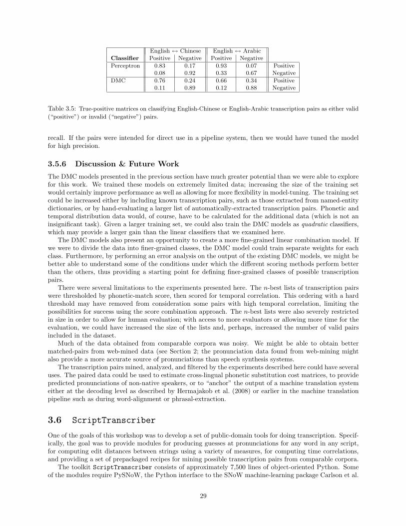
English ↔ Chinese English ↔ ArabicClassifier Positive Negative Positive Negative

Perceptron 0.83 0.17 0.93 0.07 Positive0.08 0.92 0.33 0.67 Negative

DMC 0.76 0.24 0.66 0.34 Positive0.11 0.89 0.12 0.88 Negative

Table 3.5: True-positive matrices on classifying English-Chinese or English-Arabic transcription pairs as either valid

(“positive”) or invalid (“negative”) pairs.

recall. If the pairs were intended for direct use in a pipeline system, then we would have tuned the modelfor high precision.

3.5.6 Discussion & Future Work

The DMC models presented in the previous section have much greater potential than we were able to explorefor this work. We trained these models on extremely limited data; increasing the size of the training setwould certainly improve performance as well as allowing for more flexibility in model-tuning. The training setcould be increased either by including known transcription pairs, such as those extracted from named-entitydictionaries, or by hand-evaluating a larger list of automatically-extracted transcription pairs. Phonetic andtemporal distribution data would, of course, have to be calculated for the additional data (which is not aninsignificant task). Given a larger training set, we could also train the DMC models as quadratic classifiers,which may provide a larger gain than the linear classifiers that we examined here.

The DMC models also present an opportunity to create a more fine-grained linear combination model. Ifwe were to divide the data into finer-grained classes, the DMC model could train separate weights for eachclass. Furthermore, by performing an error analysis on the output of the existing DMC models, we might bebetter able to understand some of the conditions under which the different scoring methods perform betterthan the others, thus providing a starting point for defining finer-grained classes of possible transcriptionpairs.

There were several limitations to the experiments presented here. The n-best lists of transcription pairswere thresholded by phonetic-match score, then scored for temporal correlation. This ordering with a hardthreshold may have removed from consideration some pairs with high temporal correlation, limiting thepossibilities for success using the score combination approach. The n-best lists were also severely restrictedin size in order to allow for human evaluation; with access to more evaluators or allowing more time for theevaluation, we could have increased the size of the lists and, perhaps, increased the number of valid pairsincluded in the dataset.

Much of the data obtained from comparable corpora was noisy. We might be able to obtain bettermatched-pairs from web-mined data (see Section 2; the pronunciation data found from web-mining mightalso provide a more accurate source of pronunciations than speech synthesis systems.

The transcription pairs mined, analyzed, and filtered by the experiments described here could have severaluses. The paired data could be used to estimate cross-lingual phonetic substitution cost matrices, to providepredicted pronunciations of non-native speakers, or to “anchor” the output of a machine translation systemeither at the decoding level as described by Hermajakob et al. (2008) or earlier in the machine translationpipeline such as during word-alignment or phrasal-extraction.

3.6 ScriptTranscriber

One of the goals of this workshop was to develop a set of public-domain tools for doing transcription. Specif-ically, the goal was to provide modules for producing guesses at pronunciations for any word in any script,for computing edit distances between strings using a variety of measures, for computing time correlations,and providing a set of prepackaged recipes for mining possible transcription pairs from comparable corpora.

The toolkit ScriptTranscriber consists of approximately 7,500 lines of object-oriented Python. Someof the modules require PySNoW, the Python interface to the SNoW machine-learning package Carlson et al.

29

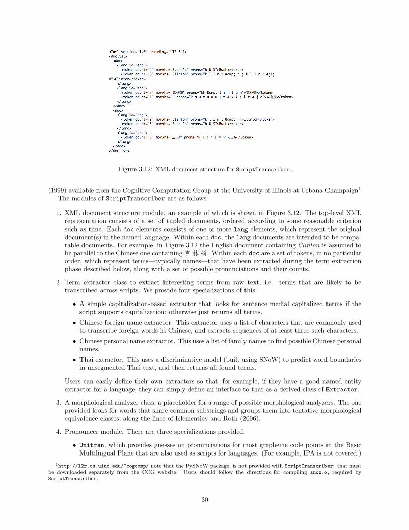
Figure 3.12: XML document structure for ScriptTranscriber.

(1999) available from the Cognitive Computation Group at the University of Illinois at Urbana-Champaign1

The modules of ScriptTranscriber are as follows:

1. XML document structure module, an example of which is shown in Figure 3.12. The top-level XMLrepresentation consists of a set of tupled documents, ordered according to some reasonable criterionsuch as time. Each doc elements consists of one or more lang elements, which represent the originaldocument(s) in the named language. Within each doc, the lang documents are intended to be compa-rable documents. For example, in Figure 3.12 the English document containing Clinton is assumed tobe parallel to the Chinese one containing克林顿. Within each doc are a set of tokens, in no particularorder, which represent terms—typically names—that have been extracted during the term extractionphase described below, along with a set of possible pronunciations and their counts.

2. Term extractor class to extract interesting terms from raw text, i.e. terms that are likely to betranscribed across scripts. We provide four specializations of this:

• A simple capitalization-based extractor that looks for sentence medial capitalized terms if thescript supports capitalization; otherwise just returns all terms.

• Chinese foreign name extractor. This extractor uses a list of characters that are commonly usedto transcribe foreign words in Chinese, and extracts sequences of at least three such characters.

• Chinese personal name extractor. This uses a list of family names to find possible Chinese personalnames.

• Thai extractor. This uses a discriminative model (built using SNoW) to predict word boundariesin unsegmented Thai text, and then returns all found terms.

Users can easily define their own extractors so that, for example, if they have a good named entityextractor for a language, they can simply define an interface to that as a derived class of Extractor.

3. A morphological analyzer class, a placeholder for a range of possible morphological analyzers. The oneprovided looks for words that share common substrings and groups them into tentative morphologicalequivalence classes, along the lines of Klementiev and Roth (2006).

4. Pronouncer module. There are three specializations provided:

• Unitran, which provides guesses on pronunciations for most grapheme code points in the BasicMultilingual Plane that are also used as scripts for languages. (For example, IPA is not covered.)

1http://l2r.cs.uiuc.edu/~cogcomp/ note that the PySNoW package, is not provided with ScriptTranscriber: that mustbe downloaded separately from the CCG website. Users should follow the directions for compiling snow.o, required byScriptTranscriber.

30

• English pronouncer: provides a Festival-derived pronunciations Taylor et al. (1998) for about 2.9million words.

• Hanzi (Chinese character) pronouncer. Provides Mandarin and Native Japanese (kunyomi) pro-nunciations for characters. Only one pronunciation prediction is provided for each character.

5. Comparator module, which provides the cost for the mapping between strings. Three specializationsare provided:

• Hand-built phonetic comparator, which uses the phonetic distance method of Tao et al. (2006);Yoon et al. (2007)

• Perceptron-based comparator, described in Section 3.4.

• Time correlation comparator, described in Section 3.5.

A sample use of the program is given on the next page. This program loads some Thai and English datafrom the distributed testdata directory, extract terms from each, builds and dumps an XML documentrepresentation, and computes phonetic distances for each pair of terms in each document.

31

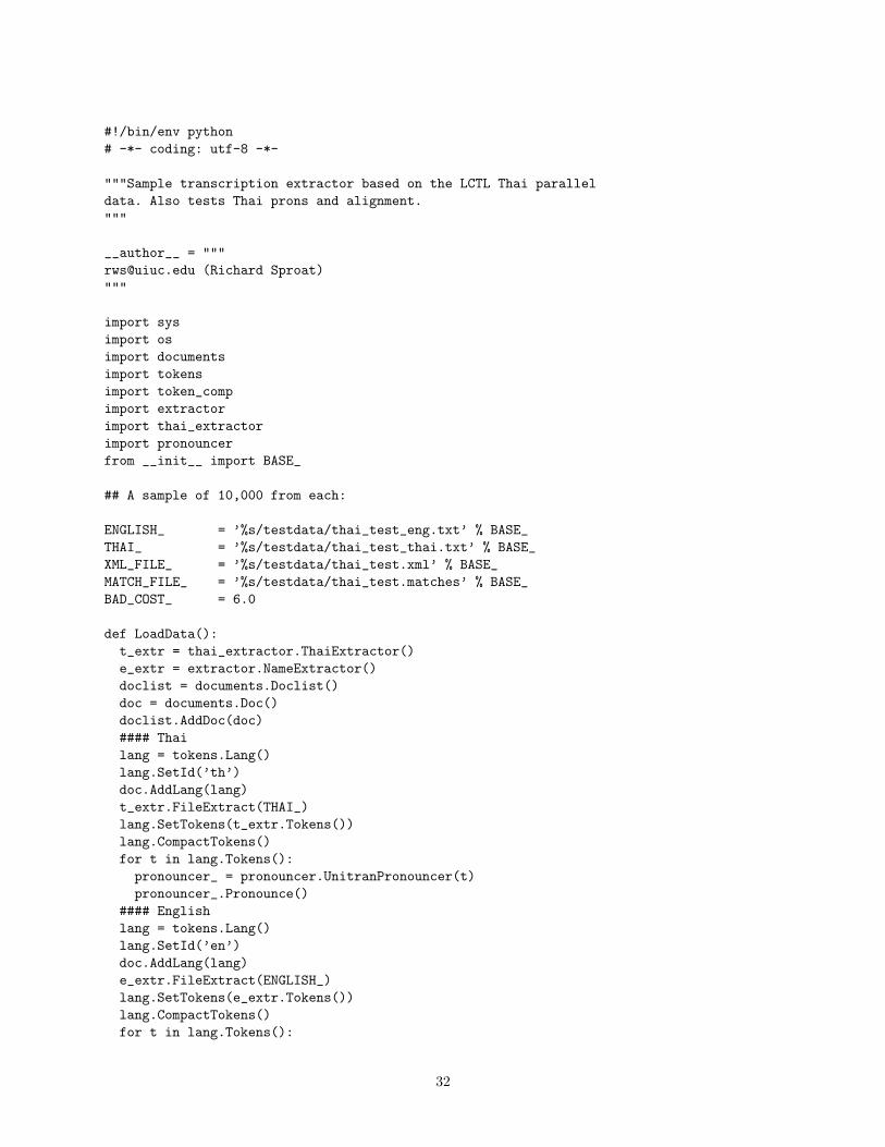
#!/bin/env python# -*- coding: utf-8 -*-

"""Sample transcription extractor based on the LCTL Thai paralleldata. Also tests Thai prons and alignment."""

__author__ = """rws@uiuc.edu (Richard Sproat)"""

import sysimport osimport documentsimport tokensimport token_compimport extractorimport thai_extractorimport pronouncerfrom __init__ import BASE_

## A sample of 10,000 from each:

ENGLISH_ = ’%s/testdata/thai_test_eng.txt’ % BASE_THAI_ = ’%s/testdata/thai_test_thai.txt’ % BASE_XML_FILE_ = ’%s/testdata/thai_test.xml’ % BASE_MATCH_FILE_ = ’%s/testdata/thai_test.matches’ % BASE_BAD_COST_ = 6.0

def LoadData():t_extr = thai_extractor.ThaiExtractor()e_extr = extractor.NameExtractor()doclist = documents.Doclist()doc = documents.Doc()doclist.AddDoc(doc)#### Thailang = tokens.Lang()lang.SetId(’th’)doc.AddLang(lang)t_extr.FileExtract(THAI_)lang.SetTokens(t_extr.Tokens())lang.CompactTokens()for t in lang.Tokens():pronouncer_ = pronouncer.UnitranPronouncer(t)pronouncer_.Pronounce()

#### Englishlang = tokens.Lang()lang.SetId(’en’)doc.AddLang(lang)e_extr.FileExtract(ENGLISH_)lang.SetTokens(e_extr.Tokens())lang.CompactTokens()for t in lang.Tokens():

32

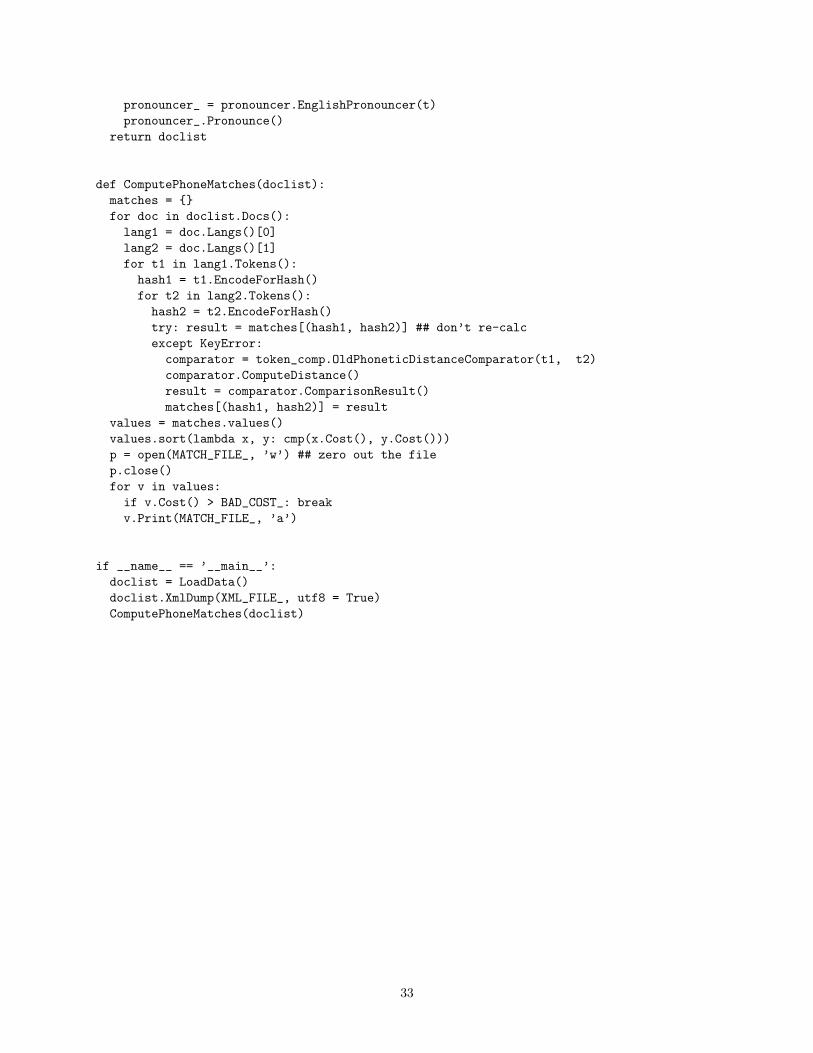
pronouncer_ = pronouncer.EnglishPronouncer(t)pronouncer_.Pronounce()

return doclist

def ComputePhoneMatches(doclist):matches = {}for doc in doclist.Docs():lang1 = doc.Langs()[0]lang2 = doc.Langs()[1]for t1 in lang1.Tokens():hash1 = t1.EncodeForHash()for t2 in lang2.Tokens():hash2 = t2.EncodeForHash()try: result = matches[(hash1, hash2)] ## don’t re-calcexcept KeyError:comparator = token_comp.OldPhoneticDistanceComparator(t1, t2)comparator.ComputeDistance()result = comparator.ComparisonResult()matches[(hash1, hash2)] = result

values = matches.values()values.sort(lambda x, y: cmp(x.Cost(), y.Cost()))p = open(MATCH_FILE_, ’w’) ## zero out the filep.close()for v in values:if v.Cost() > BAD_COST_: breakv.Print(MATCH_FILE_, ’a’)

if __name__ == ’__main__’:doclist = LoadData()doclist.XmlDump(XML_FILE_, utf8 = True)ComputePhoneMatches(doclist)

33

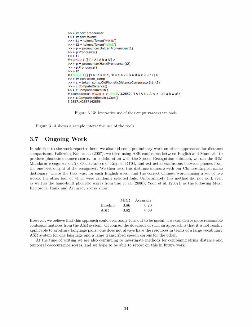
Figure 3.13: Interactive use of the ScriptTranscriber tools.

Figure 3.13 shows a sample interactive use of the tools.

3.7 Ongoing Work

In addition to the work reported here, we also did some preliminary work on other approaches for distancecomparisons. Following Kuo et al. (2007), we tried using ASR confusions between English and Mandarin toproduce phonetic distance scores. In collaboration with the Speech Recognition subteam, we ran the IBMMandarin recognizer on 2,689 utterances of English RT04, and extracted confusions between phones fromthe one-best output of the recognizer. We then used this distance measure with our Chinese-English namedictionary, where the task was, for each English word, find the correct Chinese word among a set of fivewords, the other four of which were randomly selected foils. Unfortunately this method did not work evenas well as the hand-built phonetic scores from Tao et al. (2006); Yoon et al. (2007), as the following MeanReciprocal Rank and Accuracy scores show:

MRR AccuracyBaseline 0.86 0.76ASR 0.82 0.69

However, we believe that this approach could eventually turn out to be useful, if we can derive more reasonableconfusion matrices from the ASR system. Of course, the downside of such an approach is that it is not readilyapplicable to arbitrary language pairs: one does not always have the resources in terms of a large vocabularyASR system for one language and a large transcribed speech corpus for the other.

At the time of writing we are also continuing to investigate methods for combining string distance andtemporal cooccurrence scores, and we hope to be able to report on this in future work.

34

Chapter 4

Multilingual Spoken Term Detection

The first part of the report from the speech subteam focusses on the effect of pronunciations for Out-of-Vocabulary (OOV) query terms on the performance of a spoken term detection (STD) task. OOV terms,typically proper names or foreign language terms occur infrequently but are rich in information. The STDtask returns relevant segments of speech that contain one or more of these OOV query terms. The STDsystem described here indexes word-level and subword level lattices produced by an LVCSR system usingWeighted Finite State Transducers (WFST). Experiments comparing pronunciations using n-best variationsfrom letter-to-sound rules, morphing pronunciations using phone confusions for the OOV terms and indexingone-best transcripts, lattices and confusion networks are presented. The following observations are worthmentioning: phone indexes generated from subwords represented OOVs well, too many variants for the OOVterms degrades performance if pronunciations are not weighted. Finally, we also studied the use of web-basedpronunciations.

The second part of the report addresses selecting between candidate pronunciations for out-of-vocabularywords in speech processing tasks. We introduce a simple, unsupervised method that outperforms the conven-tional supervised method of forced alignment with a reference. The success of this method is independentlydemonstrated using three metrics from large-scale speech tasks: word error rates for large vocabulary con-tinuous speech recognition, decision error tradeoff curves for spoken term detection, and phone error ratescompared to a handcrafted pronunciation lexicon. The experiments were conducted using state-of-the-artrecognition, indexing, and retrieval systems. The results were compared across many terms, hundreds ofhours of speech, and well known data sets.

4.1 Part I - Effect of Pronunciations on OOV Queries in SpokenTerm Detection

4.1.1 Introduction

The rapidly increasing amount of spoken data calls for solutions to index and search this data. Spoken termdetection (STD) is a key information retrieval technology which aims open vocabulary search over largecollections of spoken documents. The major challenge faced by STD is the lack of reliable transcriptions,an issue that becomes even more pronounced with heterogeneous, multilingual archives. Considering thefact that most STD queries consist of rare named entities or foreign words, retrieval performance is highlydependent on the recognition errors. In this context, lattice indexing provides a means of reducing the effectof recognition errors by incorporating alternative transcriptions in a probabilistic framework.

The classical approach consists of converting the speech to word transcripts using large vocabulary con-tinuous speech recognition (LVCSR) tools and extending classical Information Retrieval (IR) techniques toword transcripts. However, a significant drawback of such an approach is that search on queries containingout-of-vocabulary (OOV) terms will not return any result. These words are replaced in the output transcriptby alternatives that are probable, given the acoustic and language models of the ASR. It has been experi-mentally observed that over 10% of user queries can contain OOV terms Logan et al. (2002), as queries often

35

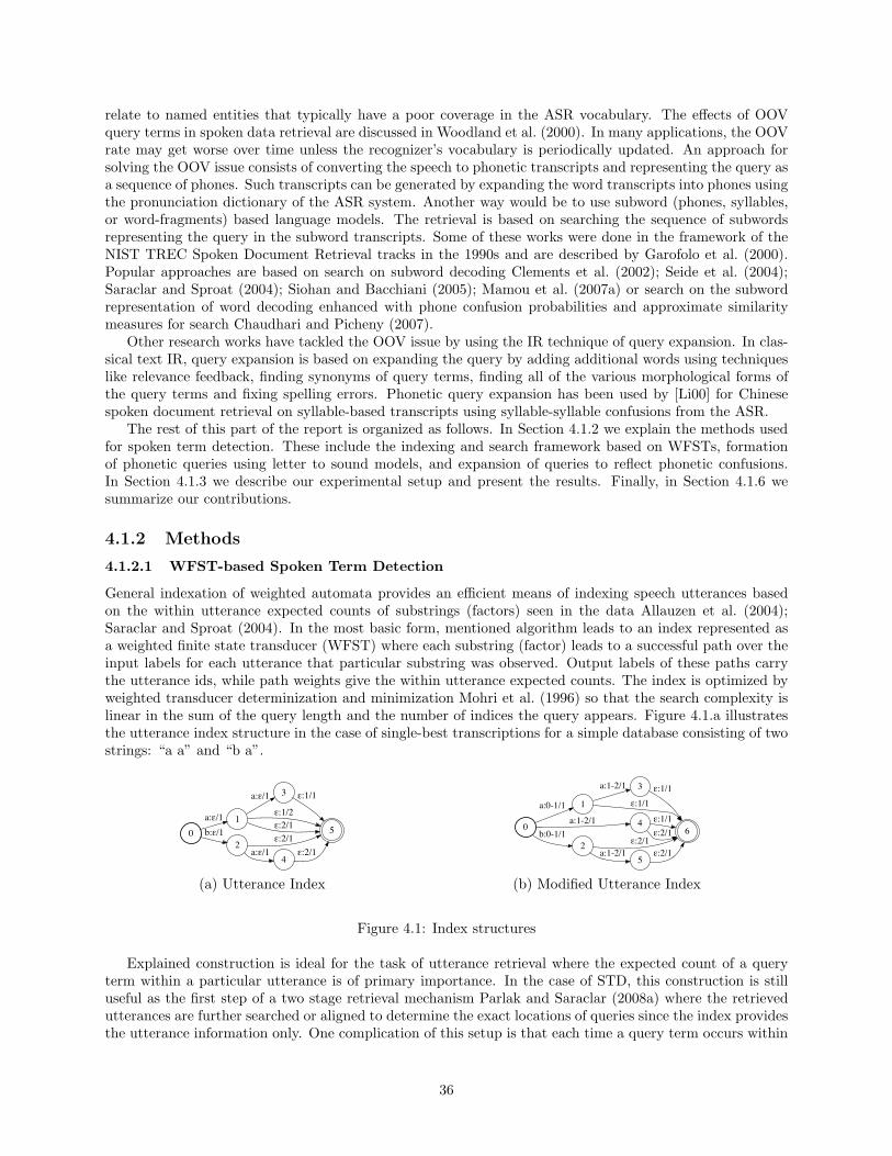
relate to named entities that typically have a poor coverage in the ASR vocabulary. The effects of OOVquery terms in spoken data retrieval are discussed in Woodland et al. (2000). In many applications, the OOVrate may get worse over time unless the recognizer’s vocabulary is periodically updated. An approach forsolving the OOV issue consists of converting the speech to phonetic transcripts and representing the query asa sequence of phones. Such transcripts can be generated by expanding the word transcripts into phones usingthe pronunciation dictionary of the ASR system. Another way would be to use subword (phones, syllables,or word-fragments) based language models. The retrieval is based on searching the sequence of subwordsrepresenting the query in the subword transcripts. Some of these works were done in the framework of theNIST TREC Spoken Document Retrieval tracks in the 1990s and are described by Garofolo et al. (2000).Popular approaches are based on search on subword decoding Clements et al. (2002); Seide et al. (2004);Saraclar and Sproat (2004); Siohan and Bacchiani (2005); Mamou et al. (2007a) or search on the subwordrepresentation of word decoding enhanced with phone confusion probabilities and approximate similaritymeasures for search Chaudhari and Picheny (2007).

Other research works have tackled the OOV issue by using the IR technique of query expansion. In clas-sical text IR, query expansion is based on expanding the query by adding additional words using techniqueslike relevance feedback, finding synonyms of query terms, finding all of the various morphological forms ofthe query terms and fixing spelling errors. Phonetic query expansion has been used by [Li00] for Chinesespoken document retrieval on syllable-based transcripts using syllable-syllable confusions from the ASR.

The rest of this part of the report is organized as follows. In Section 4.1.2 we explain the methods usedfor spoken term detection. These include the indexing and search framework based on WFSTs, formationof phonetic queries using letter to sound models, and expansion of queries to reflect phonetic confusions.In Section 4.1.3 we describe our experimental setup and present the results. Finally, in Section 4.1.6 wesummarize our contributions.

4.1.2 Methods

4.1.2.1 WFST-based Spoken Term Detection

General indexation of weighted automata provides an efficient means of indexing speech utterances basedon the within utterance expected counts of substrings (factors) seen in the data Allauzen et al. (2004);Saraclar and Sproat (2004). In the most basic form, mentioned algorithm leads to an index represented asa weighted finite state transducer (WFST) where each substring (factor) leads to a successful path over theinput labels for each utterance that particular substring was observed. Output labels of these paths carrythe utterance ids, while path weights give the within utterance expected counts. The index is optimized byweighted transducer determinization and minimization Mohri et al. (1996) so that the search complexity islinear in the sum of the query length and the number of indices the query appears. Figure 4.1.a illustratesthe utterance index structure in the case of single-best transcriptions for a simple database consisting of twostrings: “a a” and “b a”.

0

1a:!/1

2

b:!/1

3a:!/1

5

!:1/2

!:2/1

!:2/1

4a:!/1

!:1/1

!:2/1

(a) Utterance Index

0

1a:0-1/1

4a:1-2/1

2

b:0-1/1

3a:1-2/1

6

!:1/1

!:1/1

!:2/1!:2/1

5a:1-2/1

!:1/1

!:2/1

(b) Modified Utterance Index

Figure 4.1: Index structures

Explained construction is ideal for the task of utterance retrieval where the expected count of a queryterm within a particular utterance is of primary importance. In the case of STD, this construction is stilluseful as the first step of a two stage retrieval mechanism Parlak and Saraclar (2008a) where the retrievedutterances are further searched or aligned to determine the exact locations of queries since the index providesthe utterance information only. One complication of this setup is that each time a query term occurs within

36

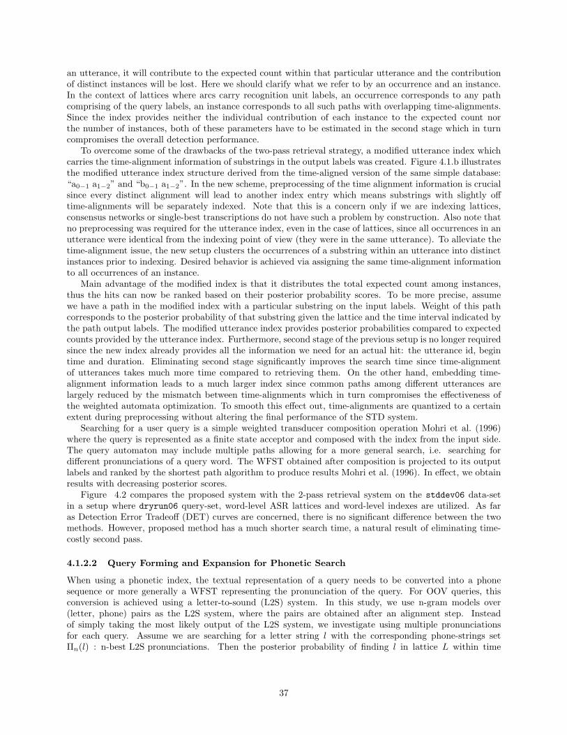
an utterance, it will contribute to the expected count within that particular utterance and the contributionof distinct instances will be lost. Here we should clarify what we refer to by an occurrence and an instance.In the context of lattices where arcs carry recognition unit labels, an occurrence corresponds to any pathcomprising of the query labels, an instance corresponds to all such paths with overlapping time-alignments.Since the index provides neither the individual contribution of each instance to the expected count northe number of instances, both of these parameters have to be estimated in the second stage which in turncompromises the overall detection performance.

To overcome some of the drawbacks of the two-pass retrieval strategy, a modified utterance index whichcarries the time-alignment information of substrings in the output labels was created. Figure 4.1.b illustratesthe modified utterance index structure derived from the time-aligned version of the same simple database:“a0−1 a1−2” and “b0−1 a1−2”. In the new scheme, preprocessing of the time alignment information is crucialsince every distinct alignment will lead to another index entry which means substrings with slightly offtime-alignments will be separately indexed. Note that this is a concern only if we are indexing lattices,consensus networks or single-best transcriptions do not have such a problem by construction. Also note thatno preprocessing was required for the utterance index, even in the case of lattices, since all occurrences in anutterance were identical from the indexing point of view (they were in the same utterance). To alleviate thetime-alignment issue, the new setup clusters the occurrences of a substring within an utterance into distinctinstances prior to indexing. Desired behavior is achieved via assigning the same time-alignment informationto all occurrences of an instance.

Main advantage of the modified index is that it distributes the total expected count among instances,thus the hits can now be ranked based on their posterior probability scores. To be more precise, assumewe have a path in the modified index with a particular substring on the input labels. Weight of this pathcorresponds to the posterior probability of that substring given the lattice and the time interval indicated bythe path output labels. The modified utterance index provides posterior probabilities compared to expectedcounts provided by the utterance index. Furthermore, second stage of the previous setup is no longer requiredsince the new index already provides all the information we need for an actual hit: the utterance id, begintime and duration. Eliminating second stage significantly improves the search time since time-alignmentof utterances takes much more time compared to retrieving them. On the other hand, embedding time-alignment information leads to a much larger index since common paths among different utterances arelargely reduced by the mismatch between time-alignments which in turn compromises the effectiveness ofthe weighted automata optimization. To smooth this effect out, time-alignments are quantized to a certainextent during preprocessing without altering the final performance of the STD system.

Searching for a user query is a simple weighted transducer composition operation Mohri et al. (1996)where the query is represented as a finite state acceptor and composed with the index from the input side.The query automaton may include multiple paths allowing for a more general search, i.e. searching fordifferent pronunciations of a query word. The WFST obtained after composition is projected to its outputlabels and ranked by the shortest path algorithm to produce results Mohri et al. (1996). In effect, we obtainresults with decreasing posterior scores.

Figure 4.2 compares the proposed system with the 2-pass retrieval system on the stddev06 data-setin a setup where dryrun06 query-set, word-level ASR lattices and word-level indexes are utilized. As faras Detection Error Tradeoff (DET) curves are concerned, there is no significant difference between the twomethods. However, proposed method has a much shorter search time, a natural result of eliminating time-costly second pass.

4.1.2.2 Query Forming and Expansion for Phonetic Search

When using a phonetic index, the textual representation of a query needs to be converted into a phonesequence or more generally a WFST representing the pronunciation of the query. For OOV queries, thisconversion is achieved using a letter-to-sound (L2S) system. In this study, we use n-gram models over(letter, phone) pairs as the L2S system, where the pairs are obtained after an alignment step. Insteadof simply taking the most likely output of the L2S system, we investigate using multiple pronunciationsfor each query. Assume we are searching for a letter string l with the corresponding phone-strings setΠn(l) : n-best L2S pronunciations. Then the posterior probability of finding l in lattice L within time

37

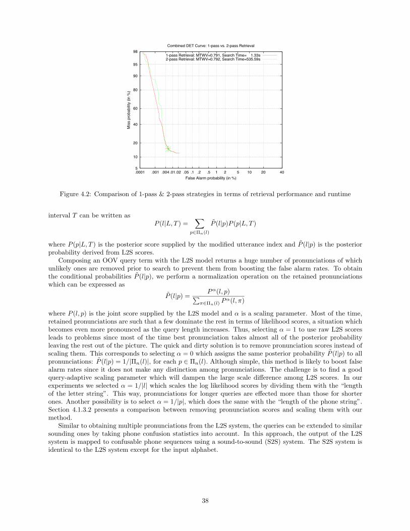
98

95

90

80

60

40

20

10

5402010521.5.2.1.05.02.01.004.001.0001

Miss

pro

babi

lity (i

n %

)

False Alarm probability (in %)

Combined DET Curve: 1-pass vs. 2-pass Retrieval

1-pass Retrieval: MTWV=0.791, Search Time= 1.33s2-pass Retrieval: MTWV=0.792, Search Time=535.59s

Figure 4.2: Comparison of 1-pass & 2-pass strategies in terms of retrieval performance and runtime

interval T can be written asP (l|L, T ) =

∑p∈Πn(l)

P (l|p)P (p|L, T )

where P (p|L, T ) is the posterior score supplied by the modified utterance index and P (l|p) is the posteriorprobability derived from L2S scores.

Composing an OOV query term with the L2S model returns a huge number of pronunciations of whichunlikely ones are removed prior to search to prevent them from boosting the false alarm rates. To obtainthe conditional probabilities P (l|p), we perform a normalization operation on the retained pronunciationswhich can be expressed as

P (l|p) =Pα(l, p)∑

π∈Πn(l) Pα(l, π)

where P (l, p) is the joint score supplied by the L2S model and α is a scaling parameter. Most of the time,retained pronunciations are such that a few dominate the rest in terms of likelihood scores, a situation whichbecomes even more pronounced as the query length increases. Thus, selecting α = 1 to use raw L2S scoresleads to problems since most of the time best pronunciation takes almost all of the posterior probabilityleaving the rest out of the picture. The quick and dirty solution is to remove pronunciation scores instead ofscaling them. This corresponds to selecting α = 0 which assigns the same posterior probability P (l|p) to allpronunciations: P (l|p) = 1/|Πn(l)|, for each p ∈ Πn(l). Although simple, this method is likely to boost falsealarm rates since it does not make any distinction among pronunciations. The challenge is to find a goodquery-adaptive scaling parameter which will dampen the large scale difference among L2S scores. In ourexperiments we selected α = 1/|l| which scales the log likelihood scores by dividing them with the “lengthof the letter string”. This way, pronunciations for longer queries are effected more than those for shorterones. Another possibility is to select α = 1/|p|, which does the same with the “length of the phone string”.Section 4.1.3.2 presents a comparison between removing pronunciation scores and scaling them with ourmethod.

Similar to obtaining multiple pronunciations from the L2S system, the queries can be extended to similarsounding ones by taking phone confusion statistics into account. In this approach, the output of the L2Ssystem is mapped to confusable phone sequences using a sound-to-sound (S2S) system. The S2S system isidentical to the L2S system except for the input alphabet.

38

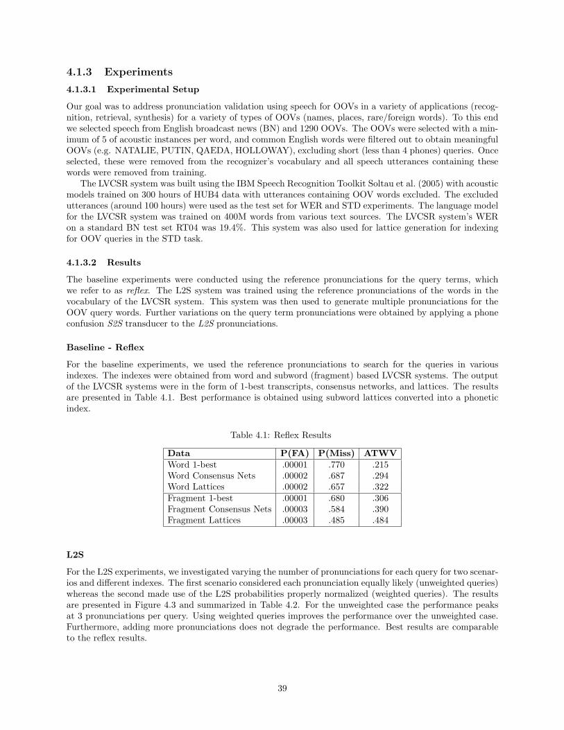
4.1.3 Experiments

4.1.3.1 Experimental Setup

Our goal was to address pronunciation validation using speech for OOVs in a variety of applications (recog-nition, retrieval, synthesis) for a variety of types of OOVs (names, places, rare/foreign words). To this endwe selected speech from English broadcast news (BN) and 1290 OOVs. The OOVs were selected with a min-imum of 5 of acoustic instances per word, and common English words were filtered out to obtain meaningfulOOVs (e.g. NATALIE, PUTIN, QAEDA, HOLLOWAY), excluding short (less than 4 phones) queries. Onceselected, these were removed from the recognizer’s vocabulary and all speech utterances containing thesewords were removed from training.

The LVCSR system was built using the IBM Speech Recognition Toolkit Soltau et al. (2005) with acousticmodels trained on 300 hours of HUB4 data with utterances containing OOV words excluded. The excludedutterances (around 100 hours) were used as the test set for WER and STD experiments. The language modelfor the LVCSR system was trained on 400M words from various text sources. The LVCSR system’s WERon a standard BN test set RT04 was 19.4%. This system was also used for lattice generation for indexingfor OOV queries in the STD task.

4.1.3.2 Results

The baseline experiments were conducted using the reference pronunciations for the query terms, whichwe refer to as reflex. The L2S system was trained using the reference pronunciations of the words in thevocabulary of the LVCSR system. This system was then used to generate multiple pronunciations for theOOV query words. Further variations on the query term pronunciations were obtained by applying a phoneconfusion S2S transducer to the L2S pronunciations.

Baseline - Reflex

For the baseline experiments, we used the reference pronunciations to search for the queries in variousindexes. The indexes were obtained from word and subword (fragment) based LVCSR systems. The outputof the LVCSR systems were in the form of 1-best transcripts, consensus networks, and lattices. The resultsare presented in Table 4.1. Best performance is obtained using subword lattices converted into a phoneticindex.

Table 4.1: Reflex Results

Data P(FA) P(Miss) ATWVWord 1-best .00001 .770 .215Word Consensus Nets .00002 .687 .294Word Lattices .00002 .657 .322Fragment 1-best .00001 .680 .306Fragment Consensus Nets .00003 .584 .390Fragment Lattices .00003 .485 .484

L2S

For the L2S experiments, we investigated varying the number of pronunciations for each query for two scenar-ios and different indexes. The first scenario considered each pronunciation equally likely (unweighted queries)whereas the second made use of the L2S probabilities properly normalized (weighted queries). The resultsare presented in Figure 4.3 and summarized in Table 4.2. For the unweighted case the performance peaksat 3 pronunciations per query. Using weighted queries improves the performance over the unweighted case.Furthermore, adding more pronunciations does not degrade the performance. Best results are comparableto the reflex results.

39

1 2 3 4 5 6 7 8 9 100.2

0.25

0.3

0.35

0.4

0.45

0.5

N

ATW

V

Fragment Lattices + Weighted L2S PronunciationsFragment Lattices + Unweighted L2S PronunciationsWord Lattices + Weighted L2S PronunciationsWord Lattices + Unweighted L2S Pronunciations

Figure 4.3: ATWV vs N-best L2S Pronunciations

Table 4.2: Best Performing N-best L2S Pronunciations

Data L2S Model # Best P(FA) P(Miss) ATWVWord Baseline 1 .00001 .796 .1901-best Weighted 6 .00004 .730 .233Word Baseline 1 .00002 .698 .281

Lattices Unweighted 3 .00005 .625 .322Weighted 6 .00005 .606 .346

Fragment Baseline 1 .00001 .757 .2291-best Weighted 10 .00005 .662 .286

Fragment Baseline 1 .00003 .597 .372Lattices Unweighted 3 .00006 .512 .425

Weighted 6 .00006 .487 .453

The DET plot for weighted L2S pronunciations using indexes obtained from fragment lattices is presentedin Figure 4.4. The single dots indicate MTWV (using a single global threshold) and ATWV (using termspecific thresholds Miller et al. (2007)) points.

98

95

90

80

60

40

20

10

5402010521.5.2.1.05.02.01.004.001.0001

Miss

pro

babi

lity (i

n %

)

False Alarm probability (in %)

Combined DET Plot: Weighted Letter-to-Sound 1-5 Best Fragment Lattices

1-best, MTWV=0.334, ATWV=0.3722-best, MTWV=0.354, ATWV=0.4223-best, MTWV=0.352, ATWV=0.4404-best, MTWV=0.339, ATWV=0.4475-best, MTWV=0.316, ATWV=0.451

Figure 4.4: Combined DET plot for weighted L2S pronunciations

40

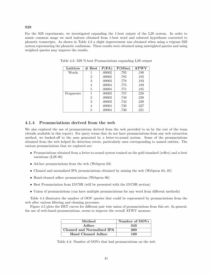
S2S

For the S2S experiments, we investigated expanding the 1-best output of the L2S system. In order tomimic common usage we used indexes obtained from 1-best word and subword hypotheses converted tophonetic transcripts. As shown in Table 4.3 a slight improvement was obtained when using a trigram S2Ssystem representing the phonetic confusions. These results were obtained using unweighted queries and usingweighted queries may improve the results.

Table 4.3: S2S N-best Pronunciations expanding L2S output

Lattices # Best P(FA) P(Miss) ATWVWords 1 .00002 .795 .190

2 .00002 .785 .1923 .00003 .778 .1934 .00004 .775 .1895 .00004 .771 .185

Fragments 1 .00002 .757 .2282 .00002 .748 .2303 .00003 .742 .2294 .00004 .738 .2275 .00004 .736 .221

4.1.4 Pronunciations derived from the web

We also explored the use of pronunciations derived from the web provided to us by the rest of the team(details available in this report). For query terms that do not have pronunciations from any web extractionmethod, we backed-off to the ones generated by a letter-to-sound system. Some of the pronunciationsobtained from the web helped fix detection errors, particularly ones corresponding to named entities. Thevarious pronunciations that we explored are:

• Pronunciations obtained from a letter-to-sound system trained on the gold standard (reflex) and n-bestvariations (L2S 00)

• Ad-hoc pronunciations from the web (Webpron 03)

• Cleaned and normalized IPA pronunciations obtained by mining the web (Webpron 04, 05)

• Hand-cleaned adhoc pronunciations (Webpron 06)

• Best Pronunciation from LVCSR (will be presented with the LVCSR section)

• Union of pronunciations (can have multiple pronunciations for any word from different methods)

Table 4.4 illustrates the number of OOV queries that could be represented by pronunciations from theweb after various filtering and cleaning processes.

Figure 4.5 plots the DET curves for different pair wise union of pronunciations from this set. In general,the use of web-based pronunciations, seems to improve the overall ATWV measure.

Method Number of OOVsAdhoc 343

Cleaned and Normalized IPA 269Hand Cleaned Adhoc 109

Table 4.4: Number of OOVs that had pronunciations on the web

41

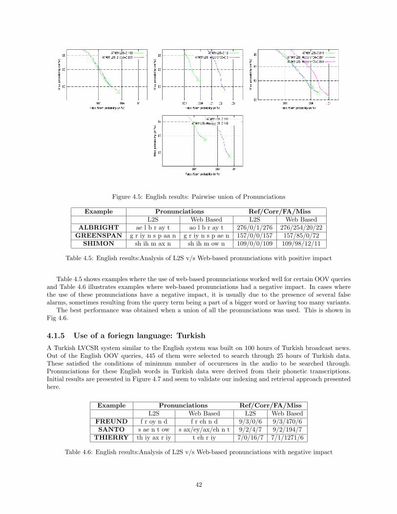
Figure 4.5: English results: Pairwise union of Pronunciations

Example Pronunciations Ref/Corr/FA/MissL2S Web Based L2S Web Based

ALBRIGHT ae l b r ay t ao l b r ay t 276/0/1/276 276/254/20/22GREENSPAN g r iy n s p aa n g r iy n s p ae n 157/0/0/157 157/85/0/72

SHIMON sh ih m ax n sh ih m ow n 109/0/0/109 109/98/12/11

Table 4.5: English results:Analysis of L2S v/s Web-based pronunciations with positive impact

Table 4.5 shows examples where the use of web-based pronunciations worked well for certain OOV queriesand Table 4.6 illustrates examples where web-based pronunciations had a negative impact. In cases wherethe use of these pronunciations have a negative impact, it is usually due to the presence of several falsealarms, sometimes resulting from the query term being a part of a bigger word or having too many variants.

The best performance was obtained when a union of all the pronunciations was used. This is shown inFig 4.6.

4.1.5 Use of a foriegn language: Turkish

A Turkish LVCSR system similar to the English system was built on 100 hours of Turkish broadcast news.Out of the English OOV queries, 445 of them were selected to search through 25 hours of Turkish data.These satisfied the conditions of minimum number of occurences in the audio to be searched through.Pronunciations for these English words in Turkish data were derived from their phonetic transcriptions.Initial results are presented in Figure 4.7 and seem to validate our indexing and retrieval approach presentedhere.

Example Pronunciations Ref/Corr/FA/MissL2S Web Based L2S Web Based

FREUND f r oy n d f r eh n d 9/3/0/6 9/3/470/6SANTO s ae n t ow s ax/ey/ax/eh n t 9/2/4/7 9/2/194/7

THIERRY th iy ax r iy t eh r iy 7/0/16/7 7/1/1271/6

Table 4.6: English results:Analysis of L2S v/s Web-based pronunciations with negative impact

42

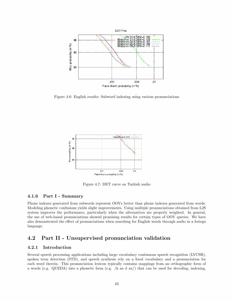
Figure 4.6: English results: Subword indexing using various pronunciations

Figure 4.7: DET curve on Turkish audio

4.1.6 Part I - Summary

Phone indexes generated from subwords represent OOVs better than phone indexes generated from words.Modeling phonetic confusions yields slight improvements. Using multiple pronunciations obtained from L2Ssystem improves the performance, particularly when the alternatives are properly weighted. In general,the use of web-based pronunciations showed promising results for certain types of OOV queries. We havealso demonstrated the effect of pronunciations when searching for English words through audio in a foriegnlanguage.

4.2 Part II - Unsupervised pronunciation validation

4.2.1 Introduction

Several speech processing applications including large vocabulary continuous speech recognition (LVCSR),spoken term detection (STD), and speech synthesis rely on a fixed vocabulary and a pronunciation foreach word therein. This pronunciation lexicon typically contains mappings from an orthographic form ofa words (e.g. QUEDA) into a phonetic form (e.g. /k aa d ax/) that can be used for decoding, indexing,

43

retrieval, or synthesis. Although the pronunciation lexicon remains fixed, realistic use requires a constantlychange vocabulary resulting in words that are out-of-vocabulary (OOV). OOVs can be new words, rarewords, foreign words, or words unknown to be important at the time the lexicon was formed. Adjusting tochange in vocabulary demands the generation of pronunciations and a need to automatically select betweencandidates. Therefore, this work addresses the question: given a word in any language, and a set of candidatepronunciations, how can you determine the best pronunciation of that word?

Challenges within OOV modeling and pronunciation validation are not new, but issues with OOV wordshave traditionally been given less attention due their low impact on word error rate (WER). Recent workWhite et al. (2008); et al. (2008) and the development of the STD task Mamou et al. (2007b) have highlightedtheir importance as rare words, which are therefore information rich.

An initial approach to create pronunciations for OOV employs a trained linguist, but they are expensive,often produce inconsistent representations, generate few pronunciations per hour, and have limited areas ofexpertise et al. (1999). Therefore effort has been made toward data-driven pronunciation modeling. Previouswork et al. (1999); Lucassen and Mercer (1984) addressing pronunciation validation comes from pronunciationmodeling attempting to simultaneously generate/validate pronunciations using existing lexica et al. (1999),linguistic rules et al. (2006), speech samples Beaufays et al. (2003); Ramabhadran et al. (1998), or all of theabove (see literature pronunciation modeling, grapheme-to-phoneme, letter-to-sound). Such work generallyincludes a criteria for creating a pronunciation for an OOV that involves the modality of data used tocreate it (e.g. generating pronunciations from lexica tests against comparisons to held out entries in thelexica, generating pronunciations from speech forced-alignment uses accuracy or WER of speech samples).The previous work on data-driven pronunciation modeling addresses pronunciation variation et al. (1999);Ramabhadran et al. (1998) or common words Lucassen and Mercer (1984); Vitale (1991). In Beaufays et al.(2003) they concentrates on names and places, directory services, noting that proper names can be hardwhere it is difficult to reuse letter-to-sound rules from common words.

For example, in Beaufays et al. (2003) they learn pronunciations from audio samples along with rules froman existing lexicon and develop an iterative algorithm for pronunciation refinement; accuracy of recognitionon directory assistance samples is measured. For many cases using speech samples including et al. (2006),the standard score comes from aligning the speech sample of a word against the putative pronunciation,sometimes with a filler model for likelihood ratio threshold. In et al. (2006) they augment acoustic likelihoodwith linguistic features and use a decision tree classifier rather than a threshold; they attempt to verifypronunciations for literacy assessment and treat the problem as estimating a confidence score over a shortutterance (the word of interest).

This work departs from the standard framework of simultaneously generating and testing pronunciations.We are agnostic about where candidates come from, isolating the task to choose between them. Furthermore,we concentrate on a large number of difficult words, of which many are foreign proper names and places.Our evaluation involves large-scale speech tasks with large data sets in an effort to present results thatgeneralize. We use two methods to select between candidate pronunciations: a conventional supervisedmethod via forced-alignment, an unsupervised method via recognition.

We compare these two methds via three metrics: phone error rate (PER) against a reference pronunciationto analyze the difference with a handcrafted lexicon, WER for LVCSR to see impact on their recognition aswell as their impact on recognizing other words in the vocabulary, and decision error tradeoff (DET) curves forSTD for searching OOVs. The end goal was to identify a methodology for picking correct pronunciations.This work was conducted as part of the Johns Hopkins University summer workshop (JHUWS08) team’Multilingual Spoken Term Detection’ where pronunciations were generated via letter-to-sound models, thoseaugmented from web data CITE, or from transliterhation models .

4.2.1.1 Baseline Supervised Method

Our baseline mechanism for choosing between two candidate pronunciations was to pick the pronunciationwith higher average acoustic likelihood from a forced-alignment with a reference, with the average taken overseveral speech samples.

Performance is measured from approximately 500 words via three metrics: edit distance to a referencelexicon, WER on decoding 100 hrs of speech, and STD DET curves on the LVCSR lattices for the same 100hours.

44

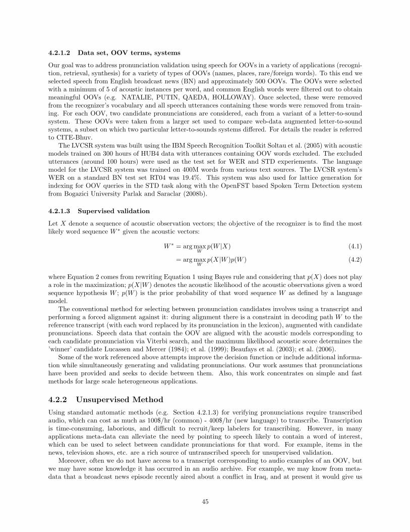
4.2.1.2 Data set, OOV terms, systems

Our goal was to address pronunciation validation using speech for OOVs in a variety of applications (recogni-tion, retrieval, synthesis) for a variety of types of OOVs (names, places, rare/foreign words). To this end weselected speech from English broadcast news (BN) and approximately 500 OOVs. The OOVs were selectedwith a minimum of 5 of acoustic instances per word, and common English words were filtered out to obtainmeaningful OOVs (e.g. NATALIE, PUTIN, QAEDA, HOLLOWAY). Once selected, these were removedfrom the recognizer’s vocabulary and all speech utterances containing these words were removed from train-ing. For each OOV, two candidate pronunciations are considered, each from a variant of a letter-to-soundsystem. These OOVs were taken from a larger set used to compare web-data augmented letter-to-soundsystems, a subset on which two particular letter-to-sounds systems differed. For details the reader is referredto CITE-Bhuv.

The LVCSR system was built using the IBM Speech Recognition Toolkit Soltau et al. (2005) with acousticmodels trained on 300 hours of HUB4 data with utterances containing OOV words excluded. The excludedutterances (around 100 hours) were used as the test set for WER and STD experiements. The languagemodel for the LVCSR system was trained on 400M words from various text sources. The LVCSR system’sWER on a standard BN test set RT04 was 19.4%. This system was also used for lattice generation forindexing for OOV queries in the STD task along with the OpenFST based Spoken Term Detection systemfrom Bogazici University Parlak and Saraclar (2008b).

4.2.1.3 Supervised validation

Let X denote a sequence of acoustic observation vectors; the objective of the recognizer is to find the mostlikely word sequence W ∗ given the acoustic vectors:

W ∗ = arg maxW

p(W |X) (4.1)

= arg maxW

p(X|W )p(W ) (4.2)

where Equation 2 comes from rewriting Equation 1 using Bayes rule and considering that p(X) does not playa role in the maximization; p(X|W ) denotes the acoustic likelihood of the acoustic observations given a wordsequence hypothesis W ; p(W ) is the prior probability of that word sequence W as defined by a languagemodel.

The conventional method for selecting between pronunciation candidates involves using a transcript andperforming a forced alignment against it: during alignment there is a constraint in decoding path W to thereference transcript (with each word replaced by its pronunciation in the lexicon), augmented with candidatepronunciations. Speech data that contain the OOV are aligned with the acoustic models corresponding toeach candidate pronunciation via Viterbi search, and the maximum likelihood acoustic score determines the’winner’ candidate Lucassen and Mercer (1984); et al. (1999); Beaufays et al. (2003); et al. (2006).

Some of the work referenced above attempts improve the decision function or include additional informa-tion while simultaneously generating and validating pronunciations. Our work assumes that pronunciationshave been provided and seeks to decide between them. Also, this work concentrates on simple and fastmethods for large scale heterogeneous applications.

4.2.2 Unsupervised Method

Using standard automatic methods (e.g. Section 4.2.1.3) for verifying pronunciations require transcribedaudio, which can cost as much as 100$/hr (common) - 400$/hr (new language) to transcribe. Transcriptionis time-consuming, laborious, and difficult to recruit/keep labelers for transcribing. However, in manyapplications meta-data can alleviate the need by pointing to speech likely to contain a word of interest,which can be used to select between candidate pronunciations for that word. For example, items in thenews, television shows, etc. are a rich source of untranscribed speech for unsupervised validation.

Moreover, often we do not have access to a transcript corresponding to audio examples of an OOV, butwe may have some knowledge it has occurred in an audio archive. For example, we may know from meta-data that a broadcast news episode recently aired about a conflict in Iraq, and at present it would give us

45

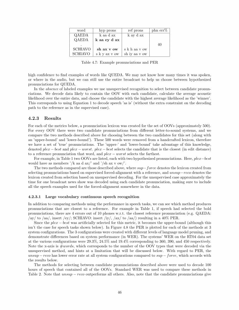
word hyp prons ref prons phn err%QAEDA k aa d ax k ay d axQAEDA k aa ey d ax

. 40SCHIAVO sh ax v ow s k h aa v owSCHIAVO s k y ax v ow sh iy aa v ow

Table 4.7: Example pronunciations and PER

high confidence to find examples of words like QUEDA. We may not know how many times it was spoken,or where in the audio, but we can still use the entire broadcast to help us choose between hypothesizedpronunciations for QUEDA.

In the absence of labeled examples we use unsupervised recognition to select between candidate pronun-ciations. We decode data likely to contain the OOV with each candidate, calculate the average acousticlikelihood over the entire data, and choose the candidate with the highest average likelihood as the ’winner’.This corresponds to using Equation 1 to decode speech ’as is’ (without the extra constraint on the decodingpath to the reference as in the supervised case).

4.2.3 Results

For each of the metrics below, a pronunciation lexicon was created for the set of OOVs (approximately 500).For every OOV there were two candidate pronunciations from different letter-to-sound systems, and wecompare the two methods described above for choosing between the two candidates for this set (along withan ’upper-bound’ and ’lower-bound’). These 500 words were removed from a handcrafted lexicon, thereforewe have a set of ’true’ pronunciations. The ’upper-’ and ’lower-bound’ take advantage of this knowledge,denoted plex− best and plex−worst. plex− best selects the candidate that is the closest (in edit distance)to a reference pronunciation that word, and plex − worst selects the farthest.

For example, in Table 1 two OOVs are listed, each with two hypothesized pronunciations. Here, plex−bestwould have as members ’/k aa d ax/’ and ’/sh ax v ow/’.

The two methods compared are those described above, where sup−force denotes the lexicon created fromselecting pronunciations based on supervised forced-alignment with a reference, and unsup−reco denotes thelexicon created from selection based on unsupervised decoding. For the unsupervised case approximately thetime for one broadcast news show was decoded using each candidate pronunciation, making sure to includeall the speech examples used for the forced-alignment somewhere in the data.

4.2.3.1 Large vocabulary continuous speech recognition

In addition to comparing methods using the performance in speech tasks, we can see which method producespronunciations that are closest to a reference. For example in Table 1, if speech had selected the boldpronunciations, there are 4 errors out of 10 phones w.r.t. the closest reference pronunciation (e.g. QAEDA:/ay/ to /aa/, insert /ey/; SCHIAVO: insert /iy/, /ax/ to /aa/) resulting in a 40% PER.

Since the plex − best was artificially selected for this metric, it becomes the upper-bound (although thisisn’t the case for speech tasks shown below). In Figure 4.8 the PER is plotted for each of the methods at 3system configurations. The 3 configurations were created with different levels of language model pruning, anddemonstrate differences based on system performance (in WER). The systems’ WER on the RT04 data setat the various configurations were 29.3%, 24.5% and 19.4% corresponding to 360, 390, and 450 respectively.Note the x-axis is #words, which corresponds to the number of the OOV types that were decoded via theunsupervised method, and hints at a limitation that will be discussed below. With regard to PER, theunsup− reco has lower error rate at all system configurations compared to sup− force, which accords withthe results below.

The methods for selecting between candidate pronunciations described above were used to decode 100hours of speech that contained all of the OOVs. Standard WER was used to compare these methods inTable 2. Note that unsup − reco outperforms all others. Also, note that the candidate pronunciations give

46

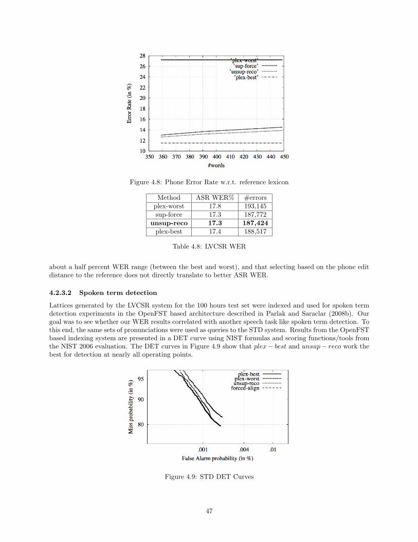
Figure 4.8: Phone Error Rate w.r.t. reference lexicon

Method ASR WER% #errorsplex-worst 17.8 193,145sup-force 17.3 187,772

unsup-reco 17.3 187,424plex-best 17.4 188,517

Table 4.8: LVCSR WER

about a half percent WER range (between the best and worst), and that selecting based on the phone editdistance to the reference does not directly translate to better ASR WER.

4.2.3.2 Spoken term detection

Lattices generated by the LVCSR system for the 100 hours test set were indexed and used for spoken termdetection experiments in the OpenFST based architecture described in Parlak and Saraclar (2008b). Ourgoal was to see whether our WER results correlated with another speech task like spoken term detection. Tothis end, the same sets of pronunciations were used as queries to the STD system. Results from the OpenFSTbased indexing system are presented in a DET curve using NIST formulas and scoring functions/tools fromthe NIST 2006 evaluation. The DET curves in Figure 4.9 show that plex− best and unsup− reco work thebest for detection at nearly all operating points.

Figure 4.9: STD DET Curves

47

4.2.4 Part II - Summary

We have presented an unsupervised method for pronunciation validation via recognition that works betterthan conventional validation via forced-alignment. This success has been demonstrated using 3 metrics forlarge-scale speech tasks: Phone Error Rate on a large set w.r.t. a reference lexicon, LVCSR Word ErrorRate on decoding a 100 hours of speech, and STD DET Curves on the same.

The usual argument for unsupervised speech methods: they save considerable time and money overspeech transcription or using a linguist, which is enticing as long as the performance degradation isn’t tooharmful. However, for selecting a candidate pronunciation our unsupervised method does not suffer anydegradation, and actually performs better as it naturally filters out unhelpful speech samples by employingthe power of comparison (search) and a language model. In all of the experiments our notion of phone errorswere based on a word-to-phone pronunciation lexicon; there were no manual phonetic transcriptions used.

There are several limitations to this method. Unsupervised recognition can’t always verify a word (ifneither pronunciation is ever decoded), although this provides a natural check against comparing many badcandidates (alignment will always give a score). It requires having seen it or words like it in text (LM),which is not unreasonable given that a word comes into fashion somehow. It’s possible that false alarmsmight hurt (if an OOV sounds like common word), but the 3 configuration experiments indicate that isn’ta problem for these words of interest. Finally, the performance could depend on amount or type of datadecoded, which is the basis of our future work.

4.3 Conclusion

Several tools were used during the course of this workshop. Speech recognition systems were built usingthe IBM speech recognition tool kit and IBM’s LVCSR decoder was used for generating lattices, N-best andconsensus networks to index the audio. An OpenFST based Indexing and Search Tool to be released shortlyas open source was developed at Bogazici University and extended during the workshop. This is an extendedimplementation of (Allauzen, Mohri and Saraclar, 2004). It can handle arbitrary fsm queries, implementsterm thresholding functions and two-pass and single-pass search for precise times of occurence of the queryterms, and provides rapid indexing and search capabilities. The key directions of research that the resultsin this workshop point to include, continued work on the multilingual aspect of using web pronunications,better ways to select pronunciations that reduce false alarms and methods to combine features from ASR(e.g. likelihood scores) and Spoken Term Detection (e.g. scores) in a classifier framework to identify thecorrect pronunciation of an OOV term.

48

Chapter 5

Acknowledgments

We wish to thank the sponsors of the 2008 workshop, including the National Science Foundation, Google,IBM, the Human Language Technology Center of Excellence (HLTCOE) at the Johns Hopkins University,and the JHU Center for Speech and Language Processing, for their support of this Workshop.

For the transcription/transliteration subteam, prior work on this project performed at the University ofIllinois at Urbana-Champaign was supported by the Department of the Interior under award NBCHC040176and by a Google Research Award.

Several individuals contributed valuable prior work to the topics investigated in this workshop. Theseinclude Su-youn Yoon, Kyoung-kyoung Kim and Tao Tao. Alex Klementiev also provided us with his softwarefor Russian-English transcription.

49

Bibliography

AbdulJaleel, N., Larkey, L., 2002. English to Arabic transliteration for information retrieval: a statisticalapproach. Tech. rep., CIIR.

AbdulJaleel, N., Larkey, L., 2003. Statistical transliteration for english-arabic cross language informationretrieval. In: CIKM’03.

Al-Onaizan, Y., Knight, K., 2002. Machine transliteration of names in Arabic text. In: Proceedings of theACL Workshop on Computational Approaches to Semitic Languages. Philadelphia, PA.

Allauzen, C., Mohri, M., Saraclar, M., 2004. General-indexation of weighted automata-application to spokenutterance retrieval. In: Proc. HLT-NAACL.

Allauzen, C., et al., 2007. OpenFST: A general and efficient weighted finite-state library. In: CIAA.

Arbabi, M., Fischthal, S., Cheng, V., Bart, E., 1994. Algorithms for Arabic name transliteration. IBMJournal of Research and Development 38 (2), 183–193.

Ballesteros, L., Croft, W. B., 1998. Resolving ambiguity for cross-language retrieval. In: Research andDevelopment in Information Retrieval. pp. 64–71.URL citeseer.ist.psu.edu/ballesteros98resolving.html

Beaufays, F., Sankar, A., Williams, S., Weintraub, M., 2003. Learning name pronunciations in automaticspeech recognition systems. In: Proc. ICTAI.

Beyerlein, P., 1998. Discriminative model combination. In: IEEE International Conference on Acoustics,Speech, and Signal Processing (ICASSP).

Bisani, M., Ney, H., 2002. Investigations on joint-multigram models for grapheme-to-phoneme conversion.In: ICSLP.

Black, A., Lenzo, K., Pagel, V., 1998. Issues in building general letter to sound rules. In: ESCA WSS-3.

Buckwalter, T., 2002. Arabic morphological analyzer version 1.0, http://www.ldc.upenn.edu/Catalog/CatalogEntry.jsp?catalogId=LDC2002L49.

Carlson, A., Cumby, C., Rosen, J., Roth, D., 1999. The SNoW learning architecture. Tech. Rep. UIUCDCS-R-99-2101, UIUC CS Dept.

Chaudhari, U. V., Picheny, M., 2007. Improvements in phone based audio search via constrained match withhigh order confusion estimates. In: Proc. of ASRU.

Clements, M., Robertson, S., Miller, M. S., 2002. Phonetic searching applied to on-line distance learningmodules. In: Proc. of IEEE Digital Signal Processing Workshop.

Cohen, W., Ravikumar, P., Fienberg, S., 2003. A comparison of string distance metrics for name-matchingtasks. In: Proceedings of the IJCAI-2003 Workshop on Information.

Dietterich, T. G., 2002. Machine learning for sequential data: A review. LNCS 2396.

50

Elovitz, H., et al., 1976. Letter-to-sound rules for automatic translation of English text to phones. IEEETrans. ASSP.

et al., J. T., 2006. Pronunciation verification of children’s speech for automatic literacy assessment. In: Proc.ICSLP.

et al., L. B., 2008. Combination of strongly and weakly constrained recognizers for reliable detection of oovs.In: Proc. ICASSP.

et al., M. R., 1999. Stochastic pronunciation modelling from hand-labelled phonetic corpora. Speech Com-munication.

Fiscus, J. G., 1997. A post-processing system to yield reduced word error rates: Recognizer output votingerror reduction (rover). In: Proceedings of the IEEE Workshop on Automatic Speech Recognition andUnderstanding. pp. 347–352.

Franz, M., McCarley, J. S., Roukos, S., 1998. Ad hoc and multilingual information retrieval at IBM. In: TextREtrieval Conference. pp. 104–115.URL citeseer.ist.psu.edu/franz99ad.html

Fung, P., 1995. A pattern matching method for finding noun and proper noun translations from noisy parallelcorpora. In: Proceedings of ACL 1995. pp. 236–243.

Gao, W., 2004. Phoneme-based statistical transliteration of foreign names for OOV problem. Master’s thesis,Chinese University of Hong Kong.

Gao, W., Wong, K.-F., Lam, W., 2004. Phoneme-based transliteration of foreign names for OOV problem.In: IJCNLP. Sanya, Hainan, pp. 374–381.

Garofolo, J. S., Auzanne, C. G. P., Voorhees, E. M., 2000. The trec spoken document retrieval track: Asuccess story. In: Proc. of TREC-9.

Goldwasser, D., Roth, D., 2008. Active sample selection for named entity transliteration. In: ACL.

Halpern, J., 2007. The challenges and pitfalls of Arabic romanization and arabization. In: ComputationalApproaches to Arabic Script Languages 2. Stanford, CA.

Hermajakob, U., Knight, K., Daume, H., 2008. Name translation in statistical machine translation: Learningwhen to transliterate. In: ACL.

Hieronymous, J., 1993. Ascii phonetic symbols for the world’s languages: Worldbet.URL citeseer.ist.psu.edu/hieronymous93ascii.html

Hollingshead, K., Fisher, S., Roark, B., October 2005. Comparing and combining finite-state and context-freeparsers. In: Proceedings of Human Language Technology Conference and Conference on Empirical Methodsin Natural Language Processing (HLT-EMNLP). Vancouver, British Columbia, Canada, pp. 787–794.

Jiang, L., Zhou, M., Chien, L.-f., Niu, C., 2007. Named entity translation with web mining and transliteration.In: IJCAI.

Kang, I., Kim, C., 2000. English-to-Korean transliteration using multiple unbounded overlapping phonemechunks. In: Proceedings of the 17th Conference on Computational Linguistics. pp. 418–424.

Kawtrkul, A., Deemagarn, A., Thumkanon, C., Khantonthong, N., McFetridge, P., 1998. Backward translit-eration for Thai document retrieval. In: 1998 IEEE Asia-Pacific Conference on Circuits and Systems. pp.563–566.

Klementiev, A., Roth, D., 2006. Weakly supervised named entity transliteration and discovery from multi-lingual comparable corpora. In: ACL.

Kneser, R., Ney, H., 1995. Improved backing-off for m-gram language modeling. In: ICASSP.

51

Knight, K., Graehl, J., 1998. Machine transliteration. CL 24 (4).

Kruskal, J., 1999. An overview of sequence comparison. In: Sankoff, D., Kruskal, J. (Eds.), Time Warps,String Edits, and Macromolecules, 2nd Edition. CSLI, Ch. 1, pp. 1–44.

Kuo, J.-S., Li, H., Yang, Y.-K., 2007. A phonetic similarity model for automatic extraction of transliterationpairs. ACM Transactions on Asian Language Information Processing.

Larkey, L., AbdulJaleel, N., Connell, M., 2003. What’s in a name?: Proper names in arabic cross languageinformation retrieval. Tech. rep., CIIR.

Lee, J., Choi, K., 1998. English to Korean statistical transliteration for information retrieval. ComputerProcessing of Oriental Languages 12 (1), 17–37.

Li, H., Sim, K. C., Kuo, J.-S., Dong, M., 2007. Semantic transliteration of personal names.

Logan, B., Moreno, P., Thong, J. V., Whittaker, E., 2002. Confusion-based query expansion for oov wordsin spoken document retreival. In: Proc. ICSLP.

Lucassen, J. M., Mercer, R. L., 1984. An information theoretic approach to the automatic determination ofphonemic baseforms. In: Proc. ICASSP.

Mamou, J., Ramabhadran, B., Siohan, O., 2007a. Vocabulary independent spoken term detection. In: Proc.of ACM SIGIR.

Mamou, J., Ramabhadran, B., Siohan, O., 2007b. Vocabulary independent spoken term detection. In: Proc.SIGIR.

Marchand, Y., Damper, R. I., 2000. A multi-strategy approach to improving pronunciation by analogy.Comp. Ling.

Masuichi, H., Flournoy, R., Kaufmann, S., Peters, S., 2000. A bootstrapping method for extracting bilingualtext pairs.URL citeseer.ist.psu.edu/masuichi00bootstrapping.html

McCallum, A., Bellare, K., Pereira, F., 2005. A conditional random field for discriminatively-trained finite-state string edit distance. In: Conference on Uncertainty in AI.

Meng, H., Lo, W., Chen, B., Tang, K., 2001. Generating phonetic cognates to handle named entities inEnglish-Chinese cross-languge spoken document retrieval. In: Proceedings of the Automatic Speech Recog-nition and Understanding Workshop.

Miller, D. R. H., Kleber, M., Kao, C., Kimball, O., Colthurst, T., Lowe, S. A., Schwartz, R. M., Gish, H.,2007. Rapid and Accurate Spoken Term Detection. In: Proc. Interspeech.

Mohri, M., Pereira, F. C. N., Riley, M., 1996. Weighted automata in text and speech processing. In: Proc.ECAI, Workshop on Extended Finite State Models of Language.

Parlak, S., Saraclar, M., 2008a. Spoken term detection for turkish broadcast news. In: Proc. ICASSP.

Parlak, S., Saraclar, M., 2008b. Spoken term detection for turkish broadcast news. In: Proc. ICASSP.

Pouliquen, B., 2008. Similarity of names across scripts: Edit distance using learned costs of n-grams. In: ??Lecture Notes in Computer Science. Springer.

Ramabhadran, B., Bahl, L. R., deSouza, P. V., Padmanabhan, M., 1998. Acoustics-only based automaticphonetic baseform generation. In: Proc. ICASSP.

Rapp, R., 1995. Identifying word translations in non-parallel texts. In: Proceedings of ACL 1995. pp. 320–322.

Ristad, E., Yianilos, P., 1998. Learning string-edit distance. IEEE Transactions on Pattern Analysis andMachine Intelligence.

52

Sadat, F., Yoshikawa, M., Uemura, S., 2003. Bilingual terminology acquisition from comparable corpora andphrasal translation to cross-language information retrieval. In: ACL ’03. pp. 141–144.

Saraclar, M., Sproat, R., 2004. Lattice-based search for spoken utterance retrieval. In: Proc. HLT-NAACL.

Seide, F., Yu, P., Ma, C., Chang, E., 2004. Vocabulary-independent search in spontaneous speech. In: Proc.of ICASSP.

Shao, L., Ng, H. T., 2004. Mining new word translations from comparable corpora. In: COLING.

Sherif, T., Kondrak, G., 2007. Bootstrapping a stochastic transducer for arabic-english transliteration ex-traction. In: ACL.

Siohan, O., Bacchiani, M., 2005. Fast vocabulary independent audio search using path based graph indexing.In: Proc. of Interspeech.

Soltau, H., Kingsbury, B., Mangu, L., Povey, D., Saon, G., Zweig, G., 2005. The ibm 2004 conversationaltelephony system for rich transcription. In: Proc. ICASSP.

Sproat, R., Tao, T., Zhai, C., July 2006. Named entity transliteration with comparable corpora. In: Pro-ceedings of COLING-ACL 2006. Sydney.

Sumita, E., Sugaya, F., 2006. Word pronunciation disambiguation using the Web. In: HLT/NAACL.

Takasu, A., Aihara, K., Yamada, T., 2007. A smoothing method for a statistical string similarity. InformationReuse and Integration.

Tanaka, K., Iwasaki, H., 1996. Extraction of lexical translation from non-aligned corpora. In: Proceedings ofCOLING 1996.

Tao, T., Yoon, S.-Y., Fister, A., Sproat, R., Zhai, C., July 2006. Unsupervised named entity transliterationusing temporal and phonetic correlation. In: EMNLP 2006. Sydney.

Tao, T., Zhai, C., 2005. Mining comparable bilingual text corpora for cross-language information integration.In: KDD’05. pp. 691–696.

Taylor, P., 2005. Hidden Markov models for grapheme to phoneme conversion. In: Interspeech.

Taylor, P., Black, A., Caley, R., 1998. The architecture of the Festival speech synthesis system. In: Proceed-ings of the Third ESCA Workshop on Speech Synthesis. Jenolan Caves, Australia, pp. 147–151.

Virga, P., Khudanpur, S., 2003. Transliteration of proper names in cross-lingual information retrieval. In:Proceedings of the ACL Workshop on Multi-lingual Named Entity Recognition.

Vitale, T., 1991. An algorithm for high accuracy name pronunciation by parametric speech synthesizer.Computational Linguistics.

White, C., Zweig, G., Burget, L., Schwarz, P., Hermansky, H., 2008. Confidence estimation, oov detection,and language id using phone-to-word transduction and phone-level alignments. In: Proc. ICASSP.

Woodland, P., Johnson, S., Jourlin, P., Jones, K. S., 2000. Effects of out of vocabulary words in spokendocument retreival. In: Proc. of ACM SIGIR.

Yang, F., Zhao, J., Zou, B., Liu, K., Liu, F., 2008. Chinese-english backward transliteration assisted withmining monolingual web pages. In: ACL.

Yoon, S.-y., Kim, K.-y., Sproat, R., 2007. Multilingual transliteration using feature based phonetic method.In: ACL.

53