EUR 24256 EN - 2010

Multimedia Assessment of Pollutant Pathways in theEnvironment, European scale model

(MAPPE-EUROPE)

Alberto Pistocchi, Grazia Zulian, Pilar Vizcaino, Dimitar Marinov

The mission of the JRC-IES is to provide scientific-technical support to the European Union’s policies for the protection and sustainable development of the European and global environment. European Commission Joint Research Centre Institute for Environment and Sustainability Contact information Address: Alberto Pistocchi, JRC, TP 460, Via Fermi 2749, 21027 Ispra (VA), Italy E-mail: alberto.pistocchi@jrc.ec.europa.eu Tel.: 00 39 0332 785591 Fax: 00 39 0332 785601 http://ies.jrc.ec.europa.eu/ http://www.jrc.ec.europa.eu/ Legal Notice Neither the European Commission nor any person acting on behalf of the Commission is responsible for the use which might be made of this publication.

Europe Direct is a service to help you find answers to your questions about the European Union

Freephone number (*):

00 800 6 7 8 9 10 11

(*) Certain mobile telephone operators do not allow access to 00 800 numbers or these calls may be billed.

A great deal of additional information on the European Union is available on the Internet. It can be accessed through the Europa server http://europa.eu/ JRC 56335 EUR 24256 EN ISBN 978-92-79-15026-5 ISSN 1018-5593 DOI 10.2788/63765 Luxembourg: Office for Official Publications of the European Communities © European Union, 2010 Reproduction is authorised provided the source is acknowledged Printed in Italy

3

1. Introduction and overview

1.1 Why spatial models of chemicals in Europe? Within the activities of the Rural, Water and Ecosystem resources (RWER) Unit of the IES during 2004-2009, a special attention was devoted to the development of a pan-European GIS based model of fate and transport of contaminants. Such model was designed for the purpose of providing spatially explicit assessment of the continental-scale trends in the environmental distribution of contaminants, capitalizing on the increasing wealth of geographic information on landscape and climate parameters which are drivers of the fate of chemicals. The spatially explicit model allows in principle the prediction of expected concentrations of chemicals at a given geographically defined location. Most of the times, however, the information on chemical emissions to the environment is not sufficiently accurate to enable reliable point-wise predictions. Under such circumstances, however, the use of spatially explicit models may be useful to derive frequency distributions of chemical concentrations, reflecting the variability of environmental parameters and emissions. In this case, maps should not be seen as geographies of contamination, but rather their histograms should be examined and presented for communication of chemical trends to the public and stakeholders. Current procedures for the authorization of chemicals in Europe rely on chemical risk assessment that is made in non-spatial terms. The procedures aim at preventing unacceptable risks from an individual emission, under “worst case scenario” assumptions. Sometimes, however, risks may arise from a combination of multiple chemicals, from multiple points or areas of emission, and they may end up affecting people or ecosystems at different locations in space. For these reasons, it may be sometimes useful to use spatially explicit models and take into account not “scenario” emissions, but “realistic” representations of actual emissions in space. Another good reason for the use of spatially explicit models is that, very often, chemical emissions are not known, while chemical concentrations are monitored at specific locations in the environment. In such cases, inverse modeling of emissions from concentrations may prove to be a very valuable exercise, and needs use of spatially explicit models to be extended. This report does not suggest that spatially explicit models should always be used, nor promotes their inclusion in current and prospective authorization procedures. Spatially explicit models are rather to be seen as assessment tools to be used wisely and having well in mind the limitations of our current understanding of chemical fate for the vast majority of substances. Recently Hollander et al., 2008, and Hollander et al., 2009, have examined in more detail the importance of both landscape/climate variability and emission variability on model results, concluding that the latter is usually much more important. Compared to the variability of physico-chemical properties among different substances, these studies highlight that landscape and climate parameters are usually less important than the type of chemical of concern, for the assessment over a relatively homogeneous area such as Europe, therefore justifying under many practical circumstances the current use of non-spatial models endorsed by the European Commission (e.g. EC,2003, EC 2004). Based on these evaluations, it can be stated that spatial models are no better than non-spatial models in capturing observed concentrations of chemicals, if the emissions are not known with sufficient approximation. Moreover, often landscape and climate parameters play a relatively unimportant role and can be replaced by default values, if one is interested in the general behavior of chemicals. However, some parameters show indeed a clear spatial pattern that may influence the fate of substances in the environment. The choice of which parameters should be considered in a spatially explicit way in modeling depends on the scale of the problem, as discussed in Pistocchi et al., 2009a. Despite the care one should take in using spatially explicit models, it is out of discussion that they are an essential tool when the focus is on the understanding of where chemicals tend to go, in space and across different media or phases.

1.2 The MAPPE modeling strategy Typically, models of various degrees of complexity have been developed, and their input has been generated through data processing in geographic information systems (GIS). An overview of existing spatial modeling approaches is presented in Pistocchi et al., 2009a. In this report, we describe a spatially explicit model that relies solely on GIS analytical functionalities, without the need of coupling GIS and external computational codes. The basic idea discussed first in

4 Pistocchi, 2005, and then, with reference to specific case studies on persistent organic pollutants (POPs), in Pistocchi, 2008a, is to generate maps of chemical emissions, maps of environmental removal rates, and eventually combine the two using map algebra to obtain estimates of chemical mass and fluxes in different media. The idea of using simple map calculations in a GIS to represent the main driving mechanisms of environmental fate and transport of chemical contaminants, as a surrogate to complex numerical models, has been the subject of extensive research and testing during the last years at the Rural, Water and Ecosystem Resources Unit of the Institute for Environment and Sustainability of the DG Joint Research Centre. Map calculations are conceptually simple, and their grounding on geographic display of input and output allows a straightforward identification of patterns, error tracking through visual inspection of input maps, on which the predictions depend, and analysis of spatial distribution of transfer and removal mechanisms, emissions, and their interplay in generating environmental concentrations. This approach proves to be also extremely simple and quick from the computational point of view. On the contrary, models describing environmental processes in much finer detail result quite often in impractical computational burdens, lack of transparence and limited capability of error tracking. For that reason the method has been chosen to assess persistent organic contaminants such as PCBs and PCDD/Fs (Pistocchi, 2008a), and Lindane (Vizcaino and Pistocchi, 2009), at the continental scale. Moreover, other chemicals have been investigated using variants of the approach, as documented in Pistocchi and Loos, 2009, with reference to perfluorinated compounds; Pistocchi et al.,2009b, with reference to pyrethroid insecticides; Pistocchi and Bidoglio, 2010, with reference to pesticides; and Pistocchi et al., 2010, with reference to household chemicals including pharmaceuticals, caffeine, and other substances of relatively high concern. In all cases, the approach has proven to yield equal or better results than existing, state-of-the-art spatially explicit models, showing that it is a level of complexity appropriate for the current understanding of chemical dynamics at the European scale. Based on the proven capability of the approach, a software has been implemented in ESRI’s ArcGIS ©, as a support tool for its routine application in future assessment activities foreseen within the European Commission JRC. There was a need to bring the available computational procedures to a well documented, user friendly and robust platform to be used by modelers. MAPPE-EUROPE is now an ArcGIS © extension for the modeling of pollutant fate and transport at continental scale using the algorithms developed within the RWER Unit at IES-JRC. The model is able to perform pipelined calculations of fate and transport of pollutants in different media. The chaining of calculations depends on the choice made by the user on the medium of original release of the pollutant (air, soil, water). Iterative calculations for the feedback loops of chemicals across media can be easily implemented by the user, also considering that often feedback fluxes are rather unimportant (Margni et al., 2004). Besides, the standardization of calculations, the software features graphical output which is easily conveyed to the end users and stakeholders.

1.3 Overview of compartment models The MAPPE modeling approach has been developed at the JRC within the FP6 Integrated Project NoMiracle (http://nomiracle.jrc.ec.europa.eu). In particular, two publicly available deliverables of the project (Pistocchi, 2005; Pistocchi, 2007) describe the conceptual development, ideas of the algorithms, and sensitivity analysis of the modeling approach. The concepts have been publicly discussed in several circumstances, and particularly in the 1st International NoMiracle workshop in Intra, Italy, in June 2006 (Pistocchi and Pennington, 2006a). The landscape and climate parameters used as default in the model were also developed within NoMiracle, and are described in a specific EUR report (Pistocchi et al., 2006). Soil water and chemical budget are described directly through simple box models of steady state mass balance and handled using map algebra. The soil water budget is computed at monthly steps according to the method developed by Pistocchi et al., 2008. Furthermore, Pistocchi, 2009, describes the monthly step soil chemical budget model implemented in MAPPE and compares it with a daily step model, showing that the two are sufficiently consistent for screening level calculations.

5 Fate and transport in lakes and the stream network, through sediment and water fluxes are described using the hydrologic functions of flow length and flow accumulation. The hydraulics of the stream network, including in particular the estimates of velocity and residence time in rivers and lakes, are described according to the methods of Pistocchi and Pennington, 2006b. The set up of the sediment compartment is based on the considerations in Pistocchi, 2008b. For the atmosphere, where dynamics is more complex, a simplified approach has been introduced, equivalent to considering average standardized contaminant concentration plumes from emissions - supposed to be uniformly proportional to population density within a country. Therefore, the atmospheric fate and transport model adopted in MAPPE is the ADEPT model, described in Roemer et al.,2005. The ADEPT model has been extensively tested as documented in Pistocchi and Galmarini, 2008; in particular, it has found to yield consistent results with the simpler, more traditional approaches used in risk assessment in Europe, having in addition the capability of yielding spatial distributions of concentrations. The seawater compartment is also developed using box models of sea zones, neglecting lateral exchanges in a way which is similar to the one for soils. The concentrations and fluxes (deposition, volatilization, loadings to the coastal zone) computed by the model are meant to represent “average” conditions consequently they reflect emissions assumed to be constant over the year (in the case of the atmosphere and inland water) or distributed monthly (in the case of soils). Moreover, environmental transfer rates are computed as annual or monthly averages based on the different environmental parameters as detailed in the remainder of this report. The developments of the model, analysis of sensitivity, limitations of the approaches adopted are discussed in the references provided in the next section. An overview scheme of the calculations the model performs is shown in Figure 1.

Figure 1 – Schematic of the MAPPE model calculations

This report focuses on the technical documentation of the software, and the user should be aware of the assumptions underpinning the approach in order to make a wise and helpful use of its output. The above mentioned literature, additional case study papers, presentations and posters, along with data sets and instructions to obtain the software are available from the MAPPE web page at http://fate.jrc.ec.europa.eu/

6

2. Detailed description of the MAPPE modeling strategy input data and algorithms

2.1 Input parameters

2.1.1 Tables Atmospheric table containing the following fields:

• Lat= latitude degrees north • Lon= longitude degrees from Greenwich • One source-receptor field for each European country • One time-of-travel field for each European country • C = concentration (ug/m3) to be computed

2.1.2 Scalar quantities • αa, βa = parameters of the temperature-degradation rate curve in air [hour-1], [-] respectively • αs, βs = parameters of the temperature-degradation rate curve in soil [hour-1], [-] respectively • αw, βw = parameters of the temperature-degradation rate curve in water [hour-1], [-]

respectively • Kow = octanol-water partitioning coefficient [-] • Kaw = air-water partitioning coefficient (non-dimensional Henry’s constant) at reference

temperature, [-] • γ = exponential coefficient of the temperature dependence of Kaw [-] • MW = molecular weight of the chemical [g/mol] • E01, E02,…, En = emission to air for each country1 [Mt/yr]

2.1.3 Maps describing landscape and climate parameters

2.1.3.1 Atmosphere

• rainfall_n - Montly Precipitation (mm/month)

• temp_n - Montly air temperature (ºC )

• pm10 - particulate in air (ug/m3), assumed to be equal to particles of diameter less than or equal

to 10 µm (PM10) • wind_

- Wind speed at 10 m (m/s) • mix_height

- Mixing layer height in the atmosphere (m)

2.1.3.2 Soil

• txt - soil texture (1: coarse; 2: medium; 3: medium-fine; 4: fine ; 5: very fine)

• etp_n

1 Emissions include direct emission, and volatilization from soils and water bodies.

7 - potential evapotranspiration (mm/month)

• octop - Organic Carbon in topsoil (% converted in number)

• erosion - Annual verage soil erosion month-1, [-]

2.1.3.3 Vegetation

• gasforest - gas deposition velocity on forest, assumed to be 0.036 m s-1 and 0.0078 ms-1 for

broadleaved and conifer forests respectively (measured gas deposition velocities in McLachlan and Horstmann, (1998). The average of the two values, 0.022 m s-1, is assigned to mixed forest. The velocities are weighted by the percentage of each type of forest derived from the CORINE Land Cover 2000 Map.

• lai_n - Monthly Life Area Index (m2/m2)

• forest - Forest (%) from the CORINE Land Cover 2000 Map

2.1.3.4 Hydrography

• z_max - Maximum catchment elevation (m)

• k_slope - exponential decay constant for stream slope [-]

• flowdirect - flow direction

• q - monthly precipitation contributing to river discharge (mm) - Slope of the 10m wind speed – particle deposition velocity relationship (m/s)

• lake_depth - Depth of lakes (m)

• vlake - flow speed in lakes (m/s)

• Mask50Km - Mask of the rivers with catchments larger than 50 km2

• Vdepn - Monthly Particle deposition velocity (m/s) obtained as a function of monthly wind speed at

10 m, and the type of underlying surface. The deposition velocity formulas and the derivation of the maps are detailed in the Appendix.

2.1.3.5 Ocean • tsm_n

- Monthly Total suspended matter in seawater (g/m3) • deph_n

- Monthly mixed layer depth in seawater (m) • STn

- Monthly surface temperature of sea water (ºC )

8 2.1.4 Emission Emissions to the atmosphere are assigned as totals per country and are treated as scalars used in the table calculation of atmospheric concentrations. The latter determines deposition from the atmosphere to soil, vegetation and water. In addition, maps of monthly emissions to soils and maps of annual emissions to water may be specified by the user. These maps should be prepared with the same spatial resolution, extent and coordinate systems as the other maps used in MAPPE, as will be explained below.

2.2 Soil water budget calculations2 The soil water balance is computed according to the method of Pistocchi et al., 2008. Formulas (ESRI ArcGIS syntax):

• compute runoff for each month (mm):

ROn = 0.25 * (([TXT] ^= 1) * 0.59 + ([TXT] == 1) * 0.47) * [Pn] + 0.75 * POW(([Pn] - 0.2 * (([TXT] ^= 1) * 250 + ([TXT] == 1) * 400)), 2) / ([Pn] + 0.8 * (([TXT] == 1) * 250 + ([TXT] ^= 1) * 400))

[ROsum] = [RO01] + [RO02] + [RO03] + [RO04] + [RO05] + [RO06] + [RO07] + [RO08] + [RO09] + [RO10] + [RO11] + [RO12]

• compute evapotranspiration for each month (mm): [ETn] = ([Pn] - [ROn]) / POW((1 + POW((([Pn] - [ROn]) / [PETn]), 1.5)), 0.6667)

• compute infiltration for each month (mm) [Fn] = [Pn] - [ETn] - [ROn]

• compute soil moisture for each month (-):

[SMn] = (([TXT] == 1) * (0.294 - 0.1765 ) + ([TXT] == 2) * (0.379 - 0.265) + ([TXT] == 3) * (0.406 - 0.2695) + ([TXT] == 4) * (0.472 - 0.3755) + ([TXT] > 4) * (0.567 - 0.451) + ([TXT] == 0) * (0.567 - 0.451)) * (1 - ([Fn] >= 0) * exp( - 0.03 * [Fn]) - ([Fn] < 0 ) * exp( - 0.3 * [Fn])) + (([TXT] == 1) * 0.1765 + ([TXT] == 2) * 0.265 + ([TXT] == 3) * 0.2695 + ([TXT] == 4) * 0.3755 + ([TXT] > 4) * 0.451 + ([TXT] == 0) * 0.451)

2.3 Hydraulic geometry and suspended sediments calculations3 The slope of the stream network is computed following an exponential profile as discussed in Pistocchi et al., 2006. The hydraulic geometry is computed according to Pistocchi and Pennington, 2006a. Suspended sediments are computed according to Hakanson et al. (2005) as discussed in Pistocchi, 2008b.

2 Calculation of runoff, evapotranspiration, infiltration and soil moisture can be done only once at the first run of the model, as these maps are not provided with installation files to save memory; for subsequent runs, the previously calculated values can be used if still existing. 3 Calculation of river velocity and depth can be done only once at the first run of the model, as these maps are not provided with installation files to save memory; for subsequent runs, the previously calculated values can be used if still existing.

9 2.3.1 Formulas (ESRI ArcGIS syntax):

• compute river slope:

[J] = [ZMax] * [Kslope] * Exp( - FlowLength([FDIR], [Kslope], UPSTREAM))

• Sum of the Infiltration of all 12 months

[Fsum] = [F01] + [F02] + [F03] + [F04] + [F05] + [F06] + [F07] + [F08] + [F09] + [F10] + [F11] + [F12]

• compute mean river width (m)

[W] = 7.3607 * POW((FlowAccumulation([FDIR], [Q], FLOAT)), 0.52425)

• compute mean river depth (m)

[h] = POW([W], (- 0.6)) * POW((FlowAccumulation([FDIR], [Q], FLOAT)), (0.6)) * POW([J], (- 0.3)) * 0.156

• compute mean river velocity (m/s)

[V] = POW([W], (-0.4)) * POW((FlowAccumulation([FDIR], [Q], FLOAT)), (0.4)) * POW([J], 0.3) * 6.428

• compute mean suspended particulate matter concentration (mg/L)

[SPM] = POW(10, (3.44 * [LatFactor] + 0.0066 * POW((FlowLength([FDIR],[one], DOWNSTREAM) / 1000) , 0.5) + 0.25 * Log10(FlowAccumulation([FDIR], [Q], FLOAT)) - 0.83))

2.4 Diffusion velocities at the air-ground interface Diffusion velocity in air and water is computed according to Schwarzenbach et al., 1993, as a function of wind speed at 10 m. Diffusion velocity in soil is computed assuming a laminar layer of air 10 mm thick, a soil pore tortuosity of 13.6 and a diffusion path bulk length in soil of 0.15 cm. Diffusivity of a generic chemical is computed from diffusivity of water in air (0.25 cm2/s) through the widely used square-root of the ratio of molecular weights.

2.4.1 Formulas (ESRI ArcGIS syntax):

• Compute air-water partition coefficient (-) for each month

[Kawn] = 'Kaw' * Exp('gamma' * ([Tn]))

• compute diffusion velocity in soil (m/s)

[DVs] = 0.000052 / POW(‘MW’, 0.5) * [mask1] • compute diffusion velocity in still water bodies (lakes, sea) (m/s)

[DVwn] = POW(32, 0.285) / POW('MW', 0.285)* (0.0000004 * POW([un], 2) + 0.000004)

• compute diffusion velocity in air (m/s)

[DVan] = POW(18, 0.335) / POW('MW', 0.335) * (0.002 * [un] + 0.003)

10 2.5 Air compartment

In its present version, the model allows to compute concentrations at any point under the assumption that emissions occur with the same spatial distribution as population density, according to the ADEPT model (Roemer et al., 2005). Concentrations are computed as the sum of the contributions from n countries:

∑=

−=n

iiii yxSRTTKEMISSyxSRRyxC

1)),(exp(),(),(

where • SRRi(x,y) is the source-receptor relation for country i-th (i.e. the concentration at point (x,y)

provoked by an emission of 1 Mt/yr of a non-decaying chemical in the country i-th) • EMISSi is the annual total emission in country i-th • SRTTi (x,y) is the time required on average for a pollutant to travel from sources in country i-th

to point (x,y) • K is the European average decay rate for the chemical (including all forms of deposition, and

atmospheric degradation). Once concentration is computed, it can be used to derive deposition fluxes to the soil and water.

2.5.1 Formulas (ESRI ArcGIS syntax):

• compute the degradation rate for each month [Kdeg_an] = 'AlfaA' * Exp('BetaA' * ([Tn])) • Compute the fraction of chemical in particulate form

[FR_AERn] = ([TSP] * 'Kow' / [Kawn] * POW(10, ( - 12.61)))/ (1 + ([TSP] * 'Kow' / [Kawn] * POW(10, ( - 12.61))))

• compute monthly particle deposition rate (wet + dry), (hr-1)

[Kdep_pn] = [FR_AERn] * (200000 * [Pn] / 86400 / 30 / 1000 + [vdepn])/ [MIX] * 3600 • compute monthly gas absorption rates, (m/s)

[out] = [LAIn] * [gasforest] [GAn] = Con (IsNull([DVs]), ([DVan] * [DVwn] / ([Kawn] * [DVan] + [DVwn])),([DVs] * (1 - [forest]) + ([out] * [forest])))

• compute monthly gas deposition rate (wet + dry), (hr-1)

[Kdep_gn] = ([Pn] / [Kawn] / 86400 / 1000 / 30 + [GAn]) * (1 - [FR_AERn]) / [MIX] * 3600

• Compute monthly overall removal rate from the atmosphere [hour-1]

[Kan] = [Kdep_pn] + [Kdep_gn] + [Kdeg_an]

• Compute the average overall removal rate4

4 From the K’atmo map, the spatial average Katmo is extracted and used as a scalar quantity in the calculation of atmospheric concentration.

11 [K1atmo] = ([Ka01] + [Ka02] + [Ka03] + [Ka04] + [Ka05] + [Ka06] + [Ka07] + [Ka08] + [Ka09] + [Ka10] + [Ka11] + [Ka12]) / 12

• Compute concentrations (µg/m3)5

[CatmoSin] = [En] * [SRn] * EXP(- [Katmo] * [TTn])

[Catmo] = Spline([inTab], conc, REGULARIZED, 0.1, 12, 1000)

• compute deposition (µg/m2/month)

[Depn] = ([Kdep_pn] + [Kdep_gn]) * [Catmo] * 30 * 24 * [MIX]

2.6 Soil compartment The mass balance is computed at steady state.

2.6.1 Formulas (ESRI ArcGIS syntax):

• compute the degradation rate for each month

[Kdeg_sn] = 'AlfaS' * Exp('BetaS' * ([Tn])) • compute soil chemical mass fractions in solid and liquid phase

a. Soil chemical mass fractions in solid phase (mean)

[par] = ([TXT] == 1) * 0.403 + ([TXT] == 2) * 0.439 + ([TXT] == 3) * 0.430 + ([TXT] == 4) * 0.520 + ([TXT] > 4) * 0.614 [Rsoln] = 0.41 * MAX([OC] / 100 , 0.001) * 'Kow' * 2.7 * (1 - [par]) / (0.41 * MAX([OC] / 100 , 0.001) * 'Kow' * 2.7 * (1 - [par]) + [SMn] + ([par] - [SMn]) * [Kawn]) [Rsol] = ([Rsol01] + [Rsol02] + [Rsol03] + [Rsol04] + [Rsol05] + [Rsol06] + [Rsol07] + [Rsol08] + [Rsol09] + [Rsol10] + [Rsol11] + [Rsol12]) / 12

b. Soil chemical mass fractions in liquid phase (mean)

[par] = ([TXT] == 1) * 0.403 + ([TXT] == 2) * 0.439 + ([TXT] == 3) * 0.430 + ([TXT] == 4) * 0.520 + ([TXT] > 4) * 0.614 [Rliqn] = 1 / (0.41 * MAX([OC] / 100 , 0.001) * 'Kow' * 2.7 * (1 - [par]) + [SMn] + ([par] - [SMn]) * [Kawn]) [Rliq] = ([Rliq01] + [Rliq02] + [Rliq03] + [Rliq04] + [Rliq05] + [Rliq06] + [Rliq07] + [Rliq08] + [Rliq09] + [Rliq10] + [Rliq11] + [Rliq12]) / 12

• compute overall removal rate (month-1)6 [par] = ([TXT] == 1) * 0.403 + ([TXT] == 2) * 0.439 + ([TXT] == 3) * 0.430 + ([TXT] == 4) * 0.520 + ([TXT] > 4) * 0.614 [Ksn] = ([Er] * [Rsoln] * [ROn] / [ROsum] / (2.7 * (1 - [par]) ) / 10000 + ([DVs] * 86400 * 30 + ([ROn] + [Fn]) / 1000) * [Rliqn]) / 0.3 + [Kdeg_sn] * 30 * 24 31_E05d Sum of deposition 5 This calculation is a table calculation in GIS. The results are then interpolated using spline and converted into a C map. The C map is used in the next steps. 6 It is assumed that soil thickness is 0.3 m.

12 • compute mass in soil (µg/m2)

[DepMean] = ([Dep01] + [Dep02] + [Dep03] + [Dep04] + [Dep05] + [Dep06] + [Dep07] + [Dep08] + [Dep09] + [Dep10] + [Dep11] + [Dep12]) / 12 [KSmean] = ((1 / [Ks01]) + (1 / [Ks02]) + (1 / [Ks03]) + (1 / [Ks04]) + (1 / [Ks05]) + (1 / [Ks06]) + (1 / [Ks07]) + (1 / [Ks08]) + (1 / [Ks09]) + (1 / [Ks10]) + (1 / [Ks11]) + (1 / [Ks12])) / 12 [Msoil]= ([DepMean] + [Qt]) * [KSmean] * (1 - [forest])

• compute concentration in the solid and liquid phases ((µg/m3)

[Cliq] = [Msoil] / 0.3 * [Rliq] [Csol] = [Msoil] / 0.3 * [Rsol]

• compute fluxes to air and water (µg /m2/month)

[Volatn] = [Cliq] * [Dn] * 86400 * 30 [Leachn] = [Cliq] * ([ROn] + (Con ([Fn] >= 0, [Fn], 0))) / 1000

2.7 Freshwater compartment (stream network including lakes) The fate and transport of the water-dissolved portion of chemicals in the stream network is described at the level of annual averages. Steady state, plug flow is assumed throughout the catchment. Under these assumptions, the equation that describes concentration (ug/m3) in surface waters (dissolved phase) is:

[ ]∫

∫−

∫

∫ ++

= ),(

),(

)(

),(_

),(_

)(

),(

),(),(),(),(),( yxL

L

dssKw

yxareacatchment

yxareacatchment

dssKw

eddQ

ddeDEPDEmissQCliqyxC

ηξηξ

ηξηξηξηξηξ ηξ

Where Cliq is the chemical concentration in dissolved phase in soil (ug/m3), DEmiss is the dissolved portion of direct emission to surface waters (ug/s/km2), DEP is atmospheric deposition (ug/s/km2), Q is unit contribution to river discharge (m3/s/km2), and Kw is the overall removal rate from surface water (m/hr). The line integral pathway L(i,j) is the flow path from generic location (i,j) to the catchment outlet. No explicit calculation of sediment-phase concentration in the stream network and lakes is done, due to the impossibility of a robust estimate at the present level of knowledge. The flux of sediment-attached chemicals is computed for each cross section of the river network or lakes as:

F = (F1 x SDR + F2)

where F1 = E x C x SDR F2 = EMISS -DEMISS

C is concentration of chemical in eroded soil (mg/t) and E is erosion rate (t/yr); DEMISS is the portion of emission EMISS which occurs in dissolved form (computed as a function of sediment concentration at the emission, under equilibrium assumptions). SDR is the sediment delivery ratio, computed according to Vanoni’s formula:

13 SDR = 0.45 A-0.125

where A is the catchment area in km2.

2.7.1 Formulas (ESRI ArcGIS syntax):

• Compute diffusion rate in water (hour-1)

[opt1]7 = 0.000046 * POW(([v]), 0.5) / POW([h], 0.5) * POW(32, 0.285) / POW('MW', 0.285) / [h] * 3600

[opt2]8 = ([DVw01] + [DVw02] + [DVw03] + [DVw04] + [DVw05] + [DVw06] + [DVw07] + [DVw08] + [DVw09] + [DVw10] + [DVw11] + [DVw12]) / 12 / [Dlake] * 3600

[DVw] = Con (IsNull([opt2]), Con (IsNull([opt1]), 0, [opt1]), [opt2])

• Compute diffusion rate in air

[DVa] = ([DVa01] + [DVa02] + [DVa03] + [DVa04] + [DVa05] + [DVa06] + [DVa07] + [DVa08] + [DVa09] + [DVa10] + [DVa11] + [DVa12]) / 12 * 3600 / [MIX]

• Compute volatilization rate (hour-1)

[KawSum] = [Kaw01] + [Kaw02] + [Kaw03] + [Kaw04] + [Kaw05] + [Kaw06] + [Kaw07] + [Kaw08] + [Kaw09] + [Kaw10] + [Kaw11] + [Kaw12]

[VOLAT] = [KawSum] / 12 * [DVa] * [DVw] / ([DVa] * [KawSum] / 12 + [DVw])

• Compute degradation rate (hour-1) 9

[Tsum] = [T01] + [T02] + [T03] + [T04] + [T05] + [T06] + [T07] + [T08] + [T09] + [T10] + [T11] + [T12]

[Kdeg_w] = 'AlfaW' * Exp('BetaW' * ([Tsum]) / 12)

• Compute dissolved fraction of direct emissions (µg/Km2)

[DEMISS] = ([EMISS] + 12 * [DepMean]) * 1000000 / (1 + 0.05 * [SPM] * 'Kow' / 1000000)

• Compute weight for flow length calculation (m)

[Weight] = ([VOLAT] + [Kdeg_w]) / (Min(Con (IsNull([V]), 0, [V]), [Vlake]) * 3600)

• Compute flow length (m)

[FL] = FlowLength([FDIR], [Weight], DOWNSTREAM)

• Compute weight for flow accumulation calculation (µg/sec)

[Weight1] = [DEMISS] / (86400 * 365) * Exp( - [FL])

7 Stream network 8 Still water 9 Considering that Kdeg follows an exponential formula dependent of temperature in centigrade degrees

14 • Compute flow accumulation (numerator) (µg/sec)

[Fa] = FlowAccumulation([FDIR], [Weight1], FLOAT)

• Compute flow accumulation (denominator) (m3/sec)

[FA1] = FlowAccumulation([FDIR], [Q], FLOAT) * 1000 / 86400 / 365

• Compute concentration, (µg/m3)

[Cwater] = Exp(LN ([Fa] / [FA1] + [FL])) * [Mask50Km]

• Compute flow accumulation weight for sediment phase flux10, 11(µg/km2/y)

[Csolsum] = [Csol01] + [Csol02] + [Csol03] + [Csol04] + [Csol05] + [Csol06] + [Csol07] + [Csol08] + [Csol09] + [Csol10] + [Csol11] + [Csol12]

[Weight2] = 100 * [Er] * [Csolsum] / 12 / 1.2 + Con (IsNull([EMISS] + [DepMean] - [DEMISS]), 0, [EMISS] + [DepMean] - [DEMISS])

• Compute sediment phase flux at each section (µg/Km2)

[F] = FlowAccumulation([FDIR], [Weight2], FLOAT)

2.8 Seawater compartment Concentration is computed from steady state balance between atmospheric deposition, on one side, and settling, volatilisation and degradation, on the other side. No direct emission is considered in oceans.

2.8.1 Formulas (ESRI ArcGIS syntax):

• Compute sediment settling removal rate (hr-1)12

[Ksettlen] = 0.0000007 * ([TSMn] / 100000000 * 0.5 * 'Kow' / (1 + [TSMn] / 100000000 * 0.5 * 'Kow')) * 3600 / [MDn]

• Compute volatilization rate (hr-1)

[Voln] = [Kawn] * [DVan] * [DVwn] / ([DVan] * [Kawn] + [DVwn]) * 3600 / [MDn] / (1 - [TSMn] / 100000000 * 'Kow' * 0.5)

• Compute degradation rate (hr-1)

[Kdeg_wn] = 'AlfaW' * Exp('BetaW' * [STn])

• Compute average overall removal rate (hr-1)

10 For simplicity, it is assumed that eroded sediment has density of 1.2 t/m3 11 Using a grid cell of 1 km2, flow accumulation with no weight provides contributing area in km2. This must be adjusted for different cell sizes. 12 A deposition velocity of 7*10E-07 m/s is assumed.

15 [Ksum] = [Kdeg_w01] + [Kdeg_w02] + [Kdeg_w03] + [Kdeg_w04] + [Kdeg_w05] + [Kdeg_w06] + [Kdeg_w07] + [Kdeg_w08] + [Kdeg_w09] + [Kdeg_w10] + [Kdeg_w11] + [Kdeg_w12] [VolSum] = [Vol01] + [Vol02] + [Vol03] + [Vol04] + [Vol05] + [Vol06] + [Vol07] + [Vol08] + [Vol09] + [Vol10] + [Vol11] + [Vol12] [KsettleSum] = [Ksettle01] + [Ksettle02] + [Ksettle03] + [Ksettle04] + [Ksettle05] + [Ksettle06] + [Ksettle07] + [Ksettle08] + [Ksettle09] + [Ksettle10] + [Ksettle11] + [Ksettle12]

[Ksw] = ([Ksum] + [VolSum] + [KsettleSum]) / 12

• Compute total load to seawater in the coast (kg/y)

[LOAD1] = Con (([coastline] == 2), [F] + ([FA1] * [Cwater] * 86400 * 365),IsNull([coastline])) * 10-9

[LOAD] = Con ([LOAD1] > 0,[LOAD1], SetNull([LOAD1]))

• Compute concentration in seawater due to deposition (µg/m3)

[MDmean] = ([MD01] + [MD02] + [MD03] + [MD04] + [MD05] + 9MD06] + [MD07] + [MD08] + [MD09] + [MD10] + [MD11] + [MD12]) / 12

[Csea] = [DepMean] / ( 24 * 30 * [Ksw] ) / [MDmean]

3. Calculation structure The following table lists the calculations above described, in terms of input and output variables and their mutual relations. Pink cells correspond to those calculations that generate outputs computed only the first time the model is run because they are independent on the chemical considered. Yellow cells correspond to those calculations that use rasters produced by other media phase. Blue cells correspond to those calculations that produce outputs that will be used by other media phase

Table 1. Table of calculation structure.

CYCLES CALCULATIONS

Com

part

men

t

Cod

AIR

SOIL

WA

TER

File

nam

es*

Des

crip

tion

Inpu

t **

Ras

ters

de

lete

d af

ter

exec

utio

n **

*

Not

es

A1 X X X RO(n) runoff [PHI], [TXT], [Pn] Produced also ROsum

A2 X X X ET(n) evapotranspiration [Pn], [PETn]

A3 X X X F(n) infiltration [Pn], [ETn], [ROn]

SO

IL W

ATER

B

ALAN

CE

A4 X X SM(n) soil moisture [TXT], [Fn]

B1 X J river slope [ZMax], [Kslope], [FDIR]

B2 X Q contribution to river mean discharge [Fn] Produced also

Fsum

B3 X W mean river width [FDIR], [Q]

B4 X H mean river depth [W], [FDIR], [Q], [J]

HYD

RAU

LIC

GE

OM

ETR

Y

B5 X V river velocity [W], [FDIR], [Q], [J]

16

Table 1. Table of calculation structure.

CYCLES CALCULATIONS C

ompa

rtm

ent

Cod

AIR

SOIL

WA

TER

File

nam

es*

Des

crip

tion

Inpu

t **

Ras

ters

de

lete

d af

ter

exec

utio

n **

*

Not

es

B6 X SPM mean suspended particulate matter concentration

[LatFactor], [FDIR], [one], [Q]

C1 X X X Kaw(n) air-water partition coefficient

Kaw', 'gamma', [Tn]

C2 X X DVs(n) diffusion velocity in soil [mask1]

C3 X X DVw(n) diffusion velocity in still water bodies MW', [un]

DIF

FUSI

ON

VE

LOC

ITIE

S

C4 X X X DVa(n) diffusion velocity in air MW', [un]

D1 X Kdeg_a(n) degradation rate AlfaA', 'BetaA', [Tn]

D2 X FR_AER(n) fraction of chemical in particulate form

[TSP], 'Kow', [Kawn]

D3 X Kdep_p(n) particle deposition rate

[FR_AERn], [Pn], [un], [vdepn], [MIX]

D4 X GA(n) gas absorption rates

[LAIn] , [gasforest], [DVan], [DVsn], [DVwn] , [Kawn], [forest]

DVs(n)

D5 X Kdep_g(n) gas deposition rate [Pn], [Kawn], [GAn], [FR_AERn], [MIX]

Kaw(n), GA(n),

FR_AER(n)

D6 X Ka(n) overall removal rate

[Kdep_pn], [Kdep_gn], [Kdeg_an]

Kdeg_a(n)

D7 X Katmo average overall removal rate [Kan] Ka(n)

D8 X Catmo concentrations [SRn], [Katmo], [TTn], [En] Katmo

AIR

D9 X Dep(n) deposition [Kdep_pn], [Kdep_gn], [Catmo], [MIX]

Kdep_p(n), Kdep_g(n)

SO

IL

E1 X Kdeg_s(n) degradation rate AlfaS', 'BetaS', [Tn]

17

Table 1. Table of calculation structure.

CYCLES CALCULATIONS C

ompa

rtm

ent

Cod

AIR

SOIL

WA

TER

File

nam

es*

Des

crip

tion

Inpu

t **

Ras

ters

de

lete

d af

ter

exec

utio

n **

*

Not

es

E2 X Rsol, Rliq chemical mass fractions in solid and liquid phase

[TXT], [OC], 'Kow', [SMn], [Kawn]

E3 X D(n) diffusion velocity (volatilization) from soil

[Kawn], [DVan], [DVsn]

Kaw(n), DVs(n)

E4 X Ks(n) overall removal rate

[TXT], [Er], [Rsoln], [ROn], [ROsum], [Dn], [Fn], [Rliqn], [Kdeg_sn]

Kdeg_s(n)

E5 X Ms mass in soil [Qt], [Depn] -[Ksn] Ks(n)

E6 X Cliq(n) and Csol(n)

concentration in the solid and liquid phases

[Msoil], [Rsoln], [Rliqn] M(n)

E7 X (VOL

+ LEACH)

Volat(n) and Leach(n)

fluxes to air and water

[Cliq], [Rsol], [Dn], [ROn], [Fn]

Rsol(n), Rliq(n),

D(n)

F1 X DVw diffusion rate in water

[v], [H], [DVwn] , [Dlake]

F2 X DVa diffusion rate in air [DVan], [MIX]

F3 X (VOL) Volat volatilization rate [Kawn], [DVa],

[DVw] DVw, DVa

F4 X Kdeg_w degradation rate [Tn], 'AlfaW', 'BetaW'

F5 X DEMISS dissolved fraction of direct emissions

[EMISS], [SPM], [SumDep], 'Kow'

F6 X Weight weight for flow length calculation

[VOLAT], [Kdeg_w], [V], [Vlake]

Kdeg_w

F7 X FL flow length [FDIR], [Weight] Weight

F8 X Weight1 weight for flow accumulation calculation

[Leachn], [DEMISS], [FL]

FRE

SH W

ATER

F9 X FA flow accumulation (numerator) [FDIR], [Weight1] Weight1

18

Table 1. Table of calculation structure.

CYCLES CALCULATIONS C

ompa

rtm

ent

Cod

AIR

SOIL

WA

TER

File

nam

es*

Des

crip

tion

Inpu

t **

Ras

ters

de

lete

d af

ter

exec

utio

n **

*

Not

es

F10 X FA1 flow accumulation (denominator) [FDIR], [Q]

F11 X Cwater concentration [Fa], [FA1], [FL], [Mask50Km] FL

F12 X Weight2 flow accumulation weight for sediment phase flux

[Csoln], [Er], [FDIR], [EMISS], [DEMISS], [Sumdep]

DEMISS

F13 X F sediment phase flux at each section [FDIR], [Weight2] Weight2

G1 X Ksettle(n) sediment settling removal rate

[TSMn], 'Kow', [MDn]

G2 X (VOL) Vol(n) volatilization rate [Kawn], [DVan],

[DVwn], [MDn] Kaw(n)

G3 X Kdeg_w(n) degradation rate AlfaW', 'BetaW', [STn]

G4 X Ksw average overall removal rate

[Kdeg_wn] [Ksettlen]

Ksettle(n), Kdeg_w(n)

G5 X LOAD total load to seawater

[Depn], [coastline], [F], [FA1], [Cwater]

FA, FA1, Cwater, F

SE

A W

ATER

G6 X Csea total concentration in seawater

[MDn]], [Ksw], [Sumdep] Ksw

TOT 17 14 30

* "(n)" means monthly ** [] = raster input, ‘ ‘ = parameters ** deleted after execution, if "Delete temporary rasters " check is selected

The following figures show the diagrams of the links between calculation maps, each represented by its identifier in the above table.

19

Figure 2 – Model of Air compartment.

20

Figure 3 – Model of Soil compartment.

21

Figure 4 – Model of Fresh Water compartment

22

Figure 5 – Model of Sea Water compartment

4. Software usage

4.1 Installation All data sets needed to run the MAPPE model are saved in ZIP format (e.g. air.zip, soil.zip and water.zip) – therefore, they have to be unzipped and and then copy in directory D:\mappe_europe_data, which is consider a default directory for the data. Similarly, the important DLL and other files which are the backbone of the MAPPE model should be copied in C:\mappe28 considered as default. The following figures aim to visually driving the user through the usage of the MAPPE software, which is itself very simple to operate. As a first step, one needs to customize the ArcMap environment in ArcGIS in order to make the MAPPE extension accessible.

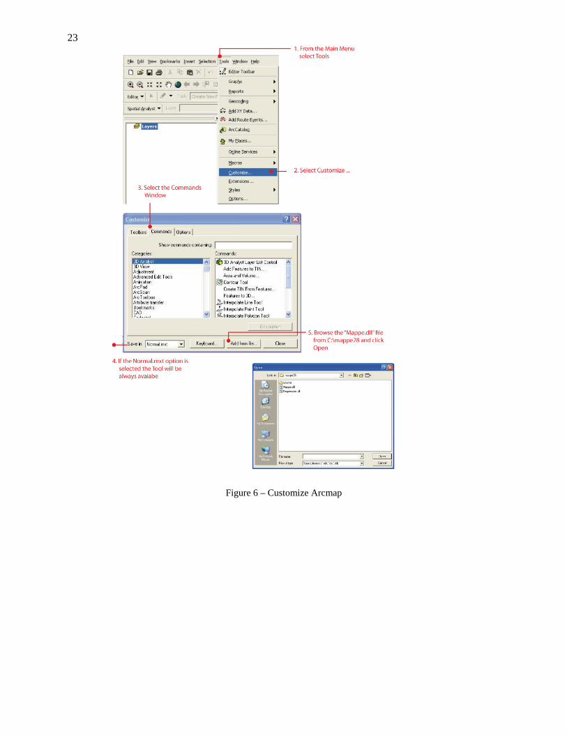
23

Figure 6 – Customize Arcmap

24

Figure 7 – Customize Arcmap (continues)

25

4.2 Prepare Data Window The “Prepare Data” form enables to indicate the paths and the filenames of the source rasters representing both chemical emission distribution and landscape and climate parameters. A short description for each raster is included. The “name” column shows exactly the label used in the formulas and can’t be changed. The “M/Y” column indicates if the measures contained in the rasters are related to a whole year (“y”) or to a single month (“m”); in this second case MAPPE expects to find 12 rasters with the same name and with a suffix from 01 to 12 (e.g. “rain01, rain02…, rain12). In the current version of MAPPE it is not possible to change the periodicity of the rasters (i.e. “Precipitation” rasters have to be montly, “soil textural class” raster has to be yearly, etc. In general the user can skip modifying these rasters except for the emissions. Only in the case when a specific input parameter needs to be changed (e.g. monthly temperature under climate change scenarios, finer resolutions for local area or regions) it can be done just by specifying the new path where data are stored. Note that all the source rasters have to be included in the indicated paths. The program won’t run a process if not all the files necessary are included and will show a message indicating which files are missing. All the source rasters are included in the DVD, and by default the path is the same path as the files are stored in the DVD. In order to increase the velocity of the whole process, is recommended to download all the data to the hard disk.

26

Figure 8 – Browsing New Input Data

27

Figure 9 – Changing Emissions Data

Unlike emissions to soil and water, emissions to air are specified as national totals, according to the ADEPT model. To specify emissions for European countries, click on the “emissions” button on the lower left corner of the window. The “European Countries” form is displayed (Figure 9) the values of the Emission to air for each country can be inserted. Values of emissions are in MT/y that leads to the computation of air concentration in µg/m3. In MAPPE 1.0 the countries names can’t be changed. NOTE: Changing input maps requires the user to ensure that the computation domain is correctly covered with data (map coordinate systems, grid extent and cell sizes). All default input data come from the dataset described in the report: Analysis of Landscape and Climate Parameters for Continental Scale Assessment of the Fate of Pollutants (Pistocchi et al, 2006) and are represented in ETRS-LAEA as proposed in the INSPIRE project (http://eusoils.jrc.it). It is recommended to keep all input maps in consistent reference systems to ensure the accuracy of the results. Once all the path for all the rasters required has been included and data of emissions to air are typed, you can move to the next step of the process, by clicking in the next step button or just clicking in the chemical management tab.

28 4.3 Chemical Management Window

To define the chemical you want to simulate, click in the chemical management tab. This form allows the management of a list of Chemicals and the selection of the chemical for which the calculation of the fate and transport model will be run. The chemical file is included in the documentation provided (chemicals.csv). Properties of the different chemicals can be changed in the chemical management form or by directly editing this file (not recommended). MAPPE comes with a list of default chemicals with given physico-chemical properties. This list is contained in the “chemicals.csv” file. Additional chemicals defined by the user can be appended to the list by clicking in the “Add’ button. This prompts the user a blank form where required properties as well as the name of the chemical and the CAS number can be typed. Once the previous steps are completed, it is possible to run the fate and transport model through the “Perform calculation” tab.

Figure 10 - Changing Chemicals Data

29

4.4 Perform Calculation Window The “Perform Calculation” form includes the commands to manage: - the calculation modality (pipelined or iterative). In case iterative calculation is selected the following parameters can also be defined: o the delta value: if the mean values calculated in two consecutive iterations differ of a value more little then delta, the calculation ends. o The maximum number of operation, after which the calculation will stop anyway. - the initial medium (Air, Soil or Water). This is the environmental compartment from which the calculation will start, and should coincide with the medium when primary emissions occur (i.e. some pesticides can be applied directly to the soil and then the process should start in the soil medium, or sprayed to air, in this case the process should start in air). Emissions for the other medium, even if null (including rasters with constant value of “0”). Have to be also included. - “Delete Intermediate Raster”: if checked, the intermediate rasters specified in the table 1 will be deleted after their use; these feature consent to reduce from 35 Gb to 20 Gb the hard disk space necessary for the executions. With this selection, of course, will not be possible anymore to visualize the intermediate rasters in ArcMap, which may be also desirable in some stages of the study (to test results of a previous step or explain further results) Pushing the “Calculate” button the calculation starts. It is possible to pause or abort the calculation process by clicking the“Pause”, “Abort” button respectively. If the calculation is paused the process that was currently running will be restarted form the beginning of this process, in the case of process calculated for every month it will mean that the process will be restarted from January. By clicking “Abort” the calculation will be interrupted and it will be necessary to restart from the beginning. The progress of the current process running as well as the progress of the overall process can be followed through the corresponding tranquilizer bars. An estimation of the computation time for each progress is also included in the calculation log. NOTE: It’s important to keep in mind that the MAPPE works with very large datasets, therefore: - Calculation times can be up to ten hours, and also calculation requires big amount of RAM memory. Consequently it’s recommended to run the process overnight. - Disk space requirements for the files can be really huge. The next tabs allow accessing utility functions such as diagram generation, export data and general settings.

30

Figure 11 - Calculation

31

Figure 12 - Progress and Calculation Log

32

4.5 Generate diagrams window This form allows to generate and to store diagrams for rasters that have associated a table. Results can be plotted as scatter diagrams or box-whiskers graphs. Additionally, descriptive statistics of the maps can be automatically extracted.

Figure 13 – Generate diagrams

33

Figure 14 – Graphical section

34

Figure 15 - Graphics section (continues)

35

Figure 16 - Graphics section (continues)

36

*.dbf Table Exemple Stat Value Count 442864.00000000000Max 0.00310000000Min 0.00020000000Mean 0.00082726684St_Dev 0.00040431305Sum 366.36670000000I_Quartile 0.00050000000Mediane 0.00070000000III_Quartile 0.00100000000

Figure 17 - Descriptive Statistics section

4.6 Export data The “Export Data” frame is useful to export the produced rasters in a format selectable between “Esri.tiff”, “ESRI.ascii” and “ESRI.float”. The rasters can be selected in a listbox as shown in the figure. Of course the raster will be selectable if already created by the calculation functionality and not already deleted by the “Delete Intermediate Raster” function. The files will be exported with the default legend and default view in which were created when running the software. The “Export” command allows to select the export path.

37

Figure 18 - Exporting Data

4.7 Settings In this form, all the information regarding the settings of the program can be selected and the default values changed. The log path refers to all the configuration files and as well as the main appl. path are established by the software and don’t need to be changed. Note that for the data path, this is just the most general path and doesn’t interfere with the detailed information that’s necessary to provide in the prepare data path. It’s important to store the results and temporary files in a disk with enough memory to store all the files generated during the run of the process. By clicking in Computed parameters, the parameter list is prompted.

38

Figure 19 - Settings

It is possible to change the formulas (and check the correctness of the syntax of the Map Algebra with the “Check Formula” button), but input raster maps can be inserted in a formula only if they are already listed under “prepare data” (i.e. no new raster can be added). This function enables adjusting formulas to test e.g. different models of phase partitioning, different values of the coefficients specified in the formulas, etc. Changes can be kept by clicking the “Save” button or original values can be recovered by clicking “Restore default”

39

Figure 20 - Change Formulas

4.8 Help A description of the input parameters and settings specified by the user appears automatically when clicking on each part of the interface. No formal on-line help is available other than the present documentation.

40

5. Example of MAPPE model application for PCBs The Polychlorinated Biphenyls (PCBs) include a large family of synthetic compounds (209 congeners) that are different in their physical-chemical and toxicological properties (Tosola et al., 1997). PCBs have been used (or still used) in wide spectra of industrial applications, e.g. dielectric fluids in capacitors and transformers, lubricating oils, plasticizers, additives to pesticides, inks and paints, etc. (Erickson, 1992). The high persistence of PCBs, their hydrophobic nature and affinity to sorption, depending of lipid and organic carbon content of particles, explain their long distance atmospheric transport and the environmental tendency to find them. Furthermore, PCBs have been found in all aquatic and marine compartments as dissolved or particulate phase in water column and sediments and in fate tissues of aquatic organisms (Dachs, 2002).

5.1 Preparation of data In this application of MAPPE for PCBs the model has been run only for one representative congener for the entire family - namely PCB153, according to Pistocchi (2008a). Data necessary to run the process with PCBs are included in the DVD. The data on emissions, physico chemical properties, all climate parameters necessary to run the model as well as the results derived from the calculation must be unzipped and downloaded before visualization. For simplicity, those data that are generic for calculations of concentrations using different pollutants are stored in the folder “data”, whereas those specific for the PCBs calculations (data of emissions, physico-chemical properties) as well as the map results are included in the folder PCBs. Data of national total emissions per year, taken from the MSCE-POP web site (Pistocchi, 2008a), are illustrated on Figure 9. Consequently the application permits to better our understanding on pan European scale level of the environmental fate of PCBs in the different media in relation with their physico-chemical properties. Furthermore, it was also developed a comparison of present model results versus data derived from monitoring campaigns and field measurements which is an additional useful test for the accuracy and efficiency of the MAPPE model. Pipe-lined mode of calculations was selected and the calculation started running from the medium air. The whole process of calculations took around 3-4 hours on 2.3MHz and 3.43GB RAM PC.

5.2 Results The presentation of the model results follow the ‘natural behavior’ of PCBs in the environment and therefore logically they are given firstly for the atmosphere followed by the simulation results for soil and surface water (streams, rivers and lakes) compartments and finally for the European seas.

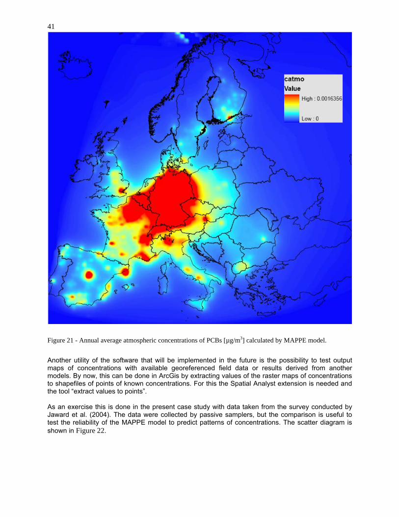
5.2.1 Atmosphere The annual average atmospheric concentrations [µg/m3] calculated by MAPPE are presented on Figure 21. Higher values of concentrations correspond to the places where emissions were higher. The general pattern of distribution follows the ADEPT model distribution that considers emissions distributed according to population density and hot spots of concentration correspond to the places of highest values of population density.

41

Figure 21 - Annual average atmospheric concentrations of PCBs [µg/m3] calculated by MAPPE model.

Another utility of the software that will be implemented in the future is the possibility to test output maps of concentrations with available georeferenced field data or results derived from another models. By now, this can be done in ArcGis by extracting values of the raster maps of concentrations to shapefiles of points of known concentrations. For this the Spatial Analyst extension is needed and the tool “extract values to points”. As an exercise this is done in the present case study with data taken from the survey conducted by Jaward et al. (2004). The data were collected by passive samplers, but the comparison is useful to test the reliability of the MAPPE model to predict patterns of concentrations. The scatter diagram is shown in Figure 22.

42

Air concentrations [ng/m3]

R2 = 0.0315

0.001

0.01

0.1

1

10

1 10 100 1000

passive sampler observations

mod

el

Figure 22 - Scatter diagram comparing air concentrations calculated by the MAPPE model vs. passive sampler observations of Jaward et al. (2004).

5.2.2 Soil compartment The pan European maps of PCBs mass in soil matrix in [µg/m3] in liquid phase and total amount are

provided in Figure 23 and Figure 24, respectively. It can be seen that higher values of mass

concentrations correspond to the places where emissions are higher (for example the areas of higher

population density). Therefore, the distribution in soil compartment is dominated by the atmospheric

patterns of PCBs but also reflects the total removal rates, showing highest values for areas with null

organic carbon content (mountainous areas) or higher precipitation rates, as well as dependence form

the wind conditions or the temperature gradients. Besides, the model performance for PCBs is tested

once more time vs. soil observations of Meijer et al. (2003) and the scatter plot is provided in Figure

25.

43

Figure 23 - European map of liquid phase of PCBs in soil matrix in [µg/m3].

44

Figure 24 - European map of total concentrations of PCBs in soil matrix in [µg/m3].

45

Soil concentrations [pg/g]

R2 = 0.6085

0.001

0.01

0.1

1

10

100

1 10 100 1000 10000 100000 1000000

observations

mod

el

Figure 25 - Scatter diagram comparing soil concentrations calculated by the MAPPE model vs. Field measurments of Meijer et al. (2004).

5.2.3 Surface water The map of concentration in water (Figure 26) represents total concentration in surface water in µg/m3

(ng/l). Similarly to the soil, the spatial distribution of PCBs in the surface water also reflects the pattern

of emission, with concentrations decaying along the river. Details could be seen, for example, on

lower scale map of Northern Italy (Figure 27). Furthermore, the model allows the riverine load of PCBs

to the European seas to be quantified (Figure 28).

46

Figure 26 - European map of total concentrations of PCBs in surface water [µg/m3].

47

Figure 27 – Details about total concentrations of PCBs in surface water [µg/m3] – Northern Italy.

48

Figure 28 – Riverine load of PCBs to the European seas [kg/year].

5.2.4 Concentrations in sea water The estimated spatial variability of PCBs concentrations [µg/m3] in the sea water is shown in Figure 29

where typical higher values could be seen in the Baltic sea close to the connection with the North

Atlantic, in the English Canal, and general close to the mouths and estuaries of the bigger European

rivers.

49

Figure 29 – Spatial variability of PCBs concentrations [ug/m3] in sea water

50

6. Appendix – derivation of the atmospheric particle deposition velocity maps

forest y = 0.0015x

soil y = 0.0005x + 0.002

water y = 0.0009x + 0.0004

0.00E+00

2.00E-03

4.00E-03

6.00E-03

8.00E-03

1.00E-02

1.20E-02

1.40E-02

1.60E-02

0 1 2 3 4 5 6 7 8

wind speed at 10 m, m s-1

depo

sitio

n ve

loci

ty, m

s-1

forestsoilwaterLinear (forest)Linear (soil)Linear (water)

Figure 30 – Regression between wind speed and deposition velocity

The deposition velocity was derived from a review of existing approaches discussed in Pistocchi,

2007. As a result of the review, it was shown that deposition velocity depended on the wind speed at

10 m through a single linear relationship for soil and sea, and a linear relationship depending on

relative humidity for forests. The slope and the intercept of the deposition velocity (y) as a function of

wind speed (x) are shown in Figure 30 the regression for forests interpolates conditions of relative

humidity of 20, 50, 80 and 100 %). The following formulas (in ESRI ArcGIS syntax) describe the

calculation conducted to obtain the two maps. In the formulas, [mask1] is a map indicating land (value

0) or sea (value 1).

• slope

Con(IsNull([forest%]), Con([mask1] == 0 , 0.0005 , 0.0009), (0.0015 * [forest%]) + ( 0.0005 *(1 -

[forest%])))

• intercept

Con(IsNull([forest%]), Con([mask1] == 0 , 0.002 , 0.0004), ( 0.002 *(1 - [forest%])))

51

7. Acknowledgements Colleagues D.Pennington, G.Bidoglio, F.Bouraoui, G.Umlauf, I.Vives-Rubio, J.Castro-Jimenez,

F.Dentener, S.Galmarini, A.Stips, F.Melin, N.Gobron and B.Pinty are gratefully acknowledged for

support with discussion, data and critical review of the work. The developers of the ADEPT model are

gratefully acknowledged for providing the data used to develop the atmospheric component of the

MAPPE model.

The software was originally developed by L.Bassi and S.Vigano’ of TXT e-solutions, Milano, Italy,

within a framework contract with the European Commission JRC. The present form of the software

was adapted by Grazia Zulian of Reggiani spa through a framework contract with the European

Commission JRC.

8. References

• Dachs J., Lohmann, R., Ockenden, W. A., Eisenreich, S.J. and Jones, K. C., 2002, Oceanic Biogeochemical Controls on Global Dynamics of Persistent Organic Pollutants. Environ. Sci. Technol. 36, 4229-4237

• EC, 2004. European Union System for the Evaluation of Substances 2.0 (EUSES 2.0). Prepared for the European Chemicals Bureau by the National Institute of Public Health andthe Environment (RIVM), Bilthoven, The Netherlands (RIVM Report no. 01900005). Available via the European Chemicals Bureau, http://ecb.jrc.it

• EC, 2003, Technical Guidance Document in support of Commission Directive 93/67/EEC on Risk Assessment for new notified substances, Commission Regulation (EC) No 1488/94 on Risk Assessment for existing substances and Directive 98/8/EC of the European Parliament and of the Council concerning the placing of biocidal products on the market. (http://ecb.jrc.it )

• Erickson, M.D., 1992. Physical, chemical, commercial, environmental and biological properties. In: Analytical chemistry of PCBs, Lewis Publishers Inc., Michigan, 1-62

• Håkanson, L. Mikrenska, M., Petrov , K. and Foster,I., 2005 Suspended particulate matter (SPM) in rivers: empirical data and models. Ecological Modelling, 183(2-3): 251-267

• Hollander A., Pistocchi A., Huijbregts M.A., Ragas A.M., Van De Meent D., 2009. Substance or space? The relative importance of substance properties and environmental characteristics in modeling the fate of chemicals in Europe. . Environmental Toxicology and Chemistry: Vol. 28, No. 1 pp. 44–51.

• Hollander, A., Hauck, M., Cousins, I., Huijbregts, M., Pistocchi, A., Ragas, A., van de Meent, D., 2009. Evaluating the utility of spatially and temporally explicit multimedia fate models, in preparation.

• Jaward F.M., Farrar, N.J, Harner, T., Sweetman, A.J., Jones, K.C., 2004, Passive Air sampling of PCBs, PBDEs, and Organochlorine Pesticides Across Europe, Environ. Sci. Technol., 2004, 38, 34-41

• Margni, M., Pennington, D.W., Bennet, D.H., Jolliet, O., 2004. Cyclic Exchanges and Level of coupling between environmental media: intermedia feedback in multimedia fate models, Environmental Science and Technology, 38, 5450-5457

• McLachlan, M., Horstmann, M., 1998. Forests as filters of airborne organic pollutants: a model Environmental Science and Technology, 1998 (32), 413-420

• Mejier, S.N., Ockenden, W.A., Sweetman, A., Breivik, K., Grimalt, J.O., Jones, K., 2003. Global distribution and budget of PCBs and HCB in background surface soils: implications for sources of Environmental processes, Environ.Sci. Technol., 2003, 37,667-672

• Pistocchi, A., 2009, On the temporal resolution of mass balance models for soluble chemicals in soils, in press, Hydrological Processes

52 • Pistocchi, A. (2008b) An assessment of soil erosion and freshwater suspended solid estimates

for continental-scale environmental modeling. Hydrological Processes, Volume 22, Issue 13, 2292-2314.

• Pistocchi, A. (2008a). A GIS-based approach for modeling the fate and transport of pollutants in Europe, Environmental Science and Technology, 42, 3640-3647

• Pistocchi, A., 2007. Report on improved multimedia fate and exposure model with various spatial resolutions at the European level, NoMiracle IP D2.4.6 technical report, 55 pp

• Pistocchi, A., 2005. Report on multimedia fate and exposure model with various spatial resolutions at the European level, NoMiracle IP D2.4.1 technical report, 62 pp

• Pistocchi, A., Bidoglio, G., 2010, Is it presently possible to assess the spatial distribution of agricultural pesticides for continental Europe? A screening study based on available data. To be submitted in 2010

• Pistocchi, A., F. Bouraoui, and M. Bittelli, 2008, A simplified parameterization of the monthly topsoil water budget, Water Resour. Res., 44, W12440, doi:10.1029/2007WR006603

• Pistocchi, A., and Galmarini, S., 2008. Evaluation of a Simple Spatially Explicit Model of Atmospheric Transport of Pollutants in Europe; in press, Environmental Modeling and Assessment, 2009. DOI: 10.1007/s10666-008-9187-x

• Pistocchi, A., R.Loos, B.Gawlik, D.Marinov, 2010, Pan-European inverse modeling to estimate the emissions of 17 common household polar chemicals. To be submitted in 2010

• Pistocchi, A., Loos, R.,A., 2009, Map of European Emissions and Concentrations of PFOS and PFOA, Environmental Science & Technology, 43 (24), 9237-9244

• Pistocchi, A., Pennington, D., 2006b. European hydraulic geometries for continental scale environmental modeling . Journal of Hydrology 329, 553–567.

• Pistocchi, A., Pennington, D.W., 2006a. Continental scale mapping of chemical fate using spatially explicit multimedia models, in Proceedings of the 1st open international NoMiracle workshop, Verbania - Intra, Italy June 8-9 2006 "Ecological and Human Health Risk Assessment: Focussing on complex chemical risk assessment and the identification of highest risk conditions"Edited by A.Pistocchi; Luxembourg: Office for Official Publications of the European Communities, EUR 22625 EN, pp 17-21, 2006.

• Pistocchi, A., D.A. Sarigiannis, P.Vizcaino, 2009a. Spatially explicit multimedia fate models for pollutants in Europe: state of the art and perspectives, in press, Science of the Total Environment

• Pistocchi, A., Vizcaino, P., Hauck, M., 2009b. A GIS model-based screening of potential contamination of soil and water by pyrethroids in Europe, Journal of Environmental Management, 90(11), 3410-3421 DOI: 10.1016/j.jenvman.2009.05.020

• Pistocchi, A., Vizcaino Martinez, M.P., Pennington, D.W., 2006. Analysis of Landscape and Climate Parameters for Continental Scale Assessment of the Fate of Pollutants; Luxembourg: Office for Official Publications of the European Communities, EUR 22624 EN, 108 pp., 2006

• Roemer, M., Baart, A., Libre, J.M., 2005. ADEPT: development of an Atmospheric Deposition and Transport model for risk assessment, TNO report B&O- A R 2005-208, Apeldoorn

• Schwarzenbach, R. P.; Gschwend, P. M.; Imboden, D. M., 1993. Environmental Organic Chemistry; Wiley: New York.

• Tosola, I., Readman, J.W., Fowler, S.W., Villeneuve, J.P., Dachs, J., Bayona, J.M. and Albaigens, J., 1997. PCBs in the western Mediterranean. Temporal trends and mass balance assessment, Deep-Sea Research II, 44 (3-4), 907-928

• Vizcaino, P., Pistocchi, A., 2009. GIS-based fate modeling of contaminants at Europe-Wide scale: case study on Lindane (γ-HCH), in preparation

53

European Commission EUR 24256 EN – Joint Research Centre – Institute for Environment and Sustainability Title: Multimedia Assessment of Pollutant Pathways in the Environment, European scale model (MAPPE-EUROPE) Author(s): Alberto Pistocchi, Grazia Zulian, Pilar Vizcaino, Dimitar Marinov Luxembourg: Office for Official Publications of the European Communities 2010 – 53 pp. – 21 x 29.7 cm EUR – Scientific and Technical Research series – ISSN 1018-5593 ISBN 978-92-79-15026-5 DOI 10.2788/63765 Abstract The report documents the structure, functions and algorithms used for the modeling of pollutant pathways in air, soil sediments and surface and sea water at the European continental scale. The algorithms are implemented in an extension for ESRI ArcGIS 9.2 a popular geographic information system (GIS) software widely used within the European Commission and in the research, environmental assessment, planning communities. The software is called MAPPE after Multimedia Assessment of Pollutant Pathways in Environment of Europe; the acronym is also the Italian word to denote maps. The purpose of the software is to provide a user-friendly way to convey the wealth of geographic data available to model the fluxes and concentrations of chemical pollutants emitted by industrial activities and other point emissions, and widespread use within households, urban environments or agriculture. The intended use is for organic contaminants such as pesticides, pharmaceuticals, VOCs, and other industrial chemicals. The output of the model, i.e. maps of concentration and chemical fluxes, can be used for the screening of hot spots at continental scale, the assessment of risk for human health and ecosystems, the evaluation of policies and scenarios with reference to the “big picture” of the continental scale. However this does not avoid the need to use more detailed, site specific assessment procedures for single problems, but provides a tool for decision support in contexts such as the management of priority substances of concern for soil, water and air quality, the control of effects of environmental pollution on human health and ecosystems, and the sustainable management of agro-chemicals, etc. by making available a geographic representation available of the consequences of emissions to air, soil and water compartments.

54

How to obtain EU publications Our priced publications are available from EU Bookshop (http://bookshop.europa.eu), where you can place an order with the sales agent of your choice. The Publications Office has a worldwide network of sales agents. You can obtain their contact details by sending a fax to (352) 29 29-42758.

55

The mission of the JRC is to provide customer-driven scientific and technical support for the conception, development, implementation and monitoring of EU policies. As a service of the European Commission, the JRC functions as a reference centre of science and technology for the Union. Close to the policy-making process, it serves the common interest of the Member States, while being independent of special interests, whether private or national.

LB-N

A-24256-E

N-C