Multimedia Databases

LSI and SVD

Text - Detailed outline

text problem full text scanning inversion signature files clustering information filtering and LSI

Information Filtering + LSI [Foltz+,’92] Goal:

users specify interests (= keywords) system alerts them, on suitable news-

documents Major contribution: LSI = Latent

Semantic Indexing latent (‘hidden’) concepts

Information Filtering + LSI

Main idea map each document into some

‘concepts’ map each term into some ‘concepts’

‘Concept’:~ a set of terms, with weights, e.g. “data” (0.8), “system” (0.5), “retrieval”

(0.6) -> DBMS_concept

Information Filtering + LSI

Pictorially: term-document matrix (BEFORE)

'data' 'system' 'retrieval' 'lung' 'ear'

TR1 1 1 1

TR2 1 1 1

TR3 1 1

TR4 1 1

Information Filtering + LSIPictorially: concept-document matrix

and...'DBMS-concept'

'medical-concept'

TR1 1

TR2 1

TR3 1

TR4 1

Information Filtering + LSI... and concept-term matrix

'DBMS-concept'

'medical-concept'

data 1

system 1

retrieval 1

lung 1

ear 1

Information Filtering + LSI

Q: How to search, eg., for ‘system’?

Information Filtering + LSIA: find the corresponding concept(s);

and the corresponding documents

'DBMS-concept'

'medical-concept'

data 1

system 1

retrieval 1

lung 1

ear 1

'DBMS-concept'

'medical-concept'

TR1 1

TR2 1

TR3 1

TR4 1

Information Filtering + LSIA: find the corresponding concept(s);

and the corresponding documents

'DBMS-concept'

'medical-concept'

data 1

system 1

retrieval 1

lung 1

ear 1

'DBMS-concept'

'medical-concept'

TR1 1

TR2 1

TR3 1

TR4 1

Information Filtering + LSI

Thus it works like an (automatically constructed) thesaurus:

we may retrieve documents that DON’T have the term ‘system’, but they contain almost everything else (‘data’, ‘retrieval’)

SVD - Detailed outline Motivation Definition - properties Interpretation Complexity Case studies Additional properties

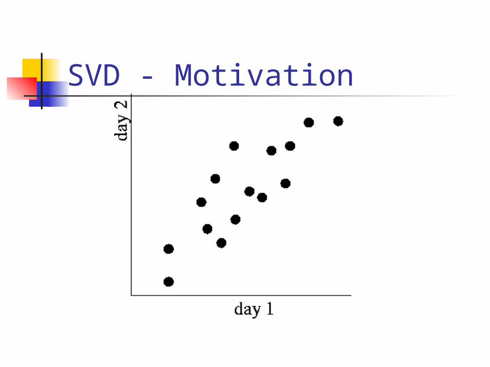
SVD - Motivation problem #1: text - LSI: find

‘concepts’ problem #2: compression / dim.

reduction

SVD - Motivation problem #1: text - LSI: find

‘concepts’

SVD - Motivation problem #2: compress / reduce

dimensionality

Problem - specs ~10**6 rows; ~10**3 columns; no updates; random access to any cell(s) ; small error: OK

SVD - Motivation

SVD - Motivation

SVD - Detailed outline Motivation Definition - properties Interpretation Complexity Case studies Additional properties

SVD - Definition

A[n x m] = U[n x r] r x r] (V[m x r])T

A: n x m matrix (eg., n documents, m terms)

U: n x r matrix (n documents, r concepts)

: r x r diagonal matrix (strength of each ‘concept’) (r : rank of the matrix)

V: m x r matrix (m terms, r concepts)

SVD - Definition A = U VT - example:

SVD - Properties

THEOREM [Press+92]: always possible to decompose matrix A into A = U VT , where

U, V: unique (*) U, V: column orthonormal (ie., columns

are unit vectors, orthogonal to each other) UT U = I; VT V = I (I: identity matrix)

: eigenvalues are positive, and sorted in decreasing order

SVD - Example A = U VT - example:

1 1 1 0 0

2 2 2 0 0

1 1 1 0 0

5 5 5 0 0

0 0 0 2 2

0 0 0 3 30 0 0 1 1

datainf.

retrieval

brain lung

0.18 0

0.36 0

0.18 0

0.90 0

0 0.53

0 0.800 0.27

=CS

MD

9.64 0

0 5.29x

0.58 0.58 0.58 0 0

0 0 0 0.71 0.71

x

SVD - Example A = U VT - example:

1 1 1 0 0

2 2 2 0 0

1 1 1 0 0

5 5 5 0 0

0 0 0 2 2

0 0 0 3 30 0 0 1 1

datainf.

retrieval

brain lung

0.18 0

0.36 0

0.18 0

0.90 0

0 0.53

0 0.800 0.27

=CS

MD

9.64 0

0 5.29x

0.58 0.58 0.58 0 0

0 0 0 0.71 0.71

x

CS-conceptMD-concept

SVD - Example A = U VT - example:

1 1 1 0 0

2 2 2 0 0

1 1 1 0 0

5 5 5 0 0

0 0 0 2 2

0 0 0 3 30 0 0 1 1

datainf.

retrieval

brain lung

0.18 0

0.36 0

0.18 0

0.90 0

0 0.53

0 0.800 0.27

=CS

MD

9.64 0

0 5.29x

0.58 0.58 0.58 0 0

0 0 0 0.71 0.71

x

CS-conceptMD-concept

doc-to-concept similarity matrix

SVD - Example A = U VT - example:

1 1 1 0 0

2 2 2 0 0

1 1 1 0 0

5 5 5 0 0

0 0 0 2 2

0 0 0 3 30 0 0 1 1

datainf.

retrieval

brain lung

0.18 0

0.36 0

0.18 0

0.90 0

0 0.53

0 0.800 0.27

=CS

MD

9.64 0

0 5.29x

0.58 0.58 0.58 0 0

0 0 0 0.71 0.71

x

‘strength’ of CS-concept

SVD - Example A = U VT - example:

1 1 1 0 0

2 2 2 0 0

1 1 1 0 0

5 5 5 0 0

0 0 0 2 2

0 0 0 3 30 0 0 1 1

datainf.

retrieval

brain lung

0.18 0

0.36 0

0.18 0

0.90 0

0 0.53

0 0.800 0.27

=CS

MD

9.64 0

0 5.29x

0.58 0.58 0.58 0 0

0 0 0 0.71 0.71

x

term-to-conceptsimilarity matrix

CS-concept

SVD - Example A = U VT - example:

1 1 1 0 0

2 2 2 0 0

1 1 1 0 0

5 5 5 0 0

0 0 0 2 2

0 0 0 3 30 0 0 1 1

datainf.

retrieval

brain lung

0.18 0

0.36 0

0.18 0

0.90 0

0 0.53

0 0.800 0.27

=CS

MD

9.64 0

0 5.29x

0.58 0.58 0.58 0 0

0 0 0 0.71 0.71

x

term-to-conceptsimilarity matrix

CS-concept

SVD - Detailed outline Motivation Definition - properties Interpretation Complexity Case studies Additional properties

SVD - Interpretation #1

‘documents’, ‘terms’ and ‘concepts’: U: document-to-concept similarity

matrix V: term-to-concept sim. matrix : its diagonal elements:

‘strength’ of each concept

SVD - Interpretation #2 best axis to project on: (‘best’ =

min sum of squares of projection errors)

SVD - Motivation

SVD - interpretation #2

minimum RMS error

SVD: givesbest axis to project

v1

SVD - Interpretation #2

SVD - Interpretation #2

A = U VT - example:

1 1 1 0 0

2 2 2 0 0

1 1 1 0 0

5 5 5 0 0

0 0 0 2 2

0 0 0 3 30 0 0 1 1

0.18 0

0.36 0

0.18 0

0.90 0

0 0.53

0 0.800 0.27

=9.64 0

0 5.29x

0.58 0.58 0.58 0 0

0 0 0 0.71 0.71

x

v1

SVD - Interpretation #2 A = U VT - example:

1 1 1 0 0

2 2 2 0 0

1 1 1 0 0

5 5 5 0 0

0 0 0 2 2

0 0 0 3 30 0 0 1 1

0.18 0

0.36 0

0.18 0

0.90 0

0 0.53

0 0.800 0.27

=9.64 0

0 5.29x

0.58 0.58 0.58 0 0

0 0 0 0.71 0.71

x

variance (‘spread’) on the v1 axis

SVD - Interpretation #2 A = U VT - example:

U gives the coordinates of the points in the projection axis

1 1 1 0 0

2 2 2 0 0

1 1 1 0 0

5 5 5 0 0

0 0 0 2 2

0 0 0 3 30 0 0 1 1

0.18 0

0.36 0

0.18 0

0.90 0

0 0.53

0 0.800 0.27

=9.64 0

0 5.29x

0.58 0.58 0.58 0 0

0 0 0 0.71 0.71

x

SVD - Interpretation #2 More details Q: how exactly is dim. reduction

done?1 1 1 0 0

2 2 2 0 0

1 1 1 0 0

5 5 5 0 0

0 0 0 2 2

0 0 0 3 30 0 0 1 1

0.18 0

0.36 0

0.18 0

0.90 0

0 0.53

0 0.800 0.27

=9.64 0

0 5.29x

0.58 0.58 0.58 0 0

0 0 0 0.71 0.71

x

SVD - Interpretation #2 More details Q: how exactly is dim. reduction

done? A: set the smallest eigenvalues to

zero:1 1 1 0 0

2 2 2 0 0

1 1 1 0 0

5 5 5 0 0

0 0 0 2 2

0 0 0 3 30 0 0 1 1

0.18 0

0.36 0

0.18 0

0.90 0

0 0.53

0 0.800 0.27

=9.64 0

0 5.29x

0.58 0.58 0.58 0 0

0 0 0 0.71 0.71

x

SVD - Interpretation #2

1 1 1 0 0

2 2 2 0 0

1 1 1 0 0

5 5 5 0 0

0 0 0 2 2

0 0 0 3 30 0 0 1 1

0.18 0

0.36 0

0.18 0

0.90 0

0 0.53

0 0.800 0.27

~9.64 0

0 0x

0.58 0.58 0.58 0 0

0 0 0 0.71 0.71

x

SVD - Interpretation #2

1 1 1 0 0

2 2 2 0 0

1 1 1 0 0

5 5 5 0 0

0 0 0 2 2

0 0 0 3 30 0 0 1 1

0.18 0

0.36 0

0.18 0

0.90 0

0 0.53

0 0.800 0.27

~9.64 0

0 0x

0.58 0.58 0.58 0 0

0 0 0 0.71 0.71

x

SVD - Interpretation #2

1 1 1 0 0

2 2 2 0 0

1 1 1 0 0

5 5 5 0 0

0 0 0 2 2

0 0 0 3 30 0 0 1 1

0.18

0.36

0.18

0.90

0

00

~9.64

x

0.58 0.58 0.58 0 0

x

SVD - Interpretation #2

1 1 1 0 0

2 2 2 0 0

1 1 1 0 0

5 5 5 0 0

0 0 0 2 2

0 0 0 3 30 0 0 1 1

~

1 1 1 0 0

2 2 2 0 0

1 1 1 0 0

5 5 5 0 0

0 0 0 0 0

0 0 0 0 00 0 0 0 0

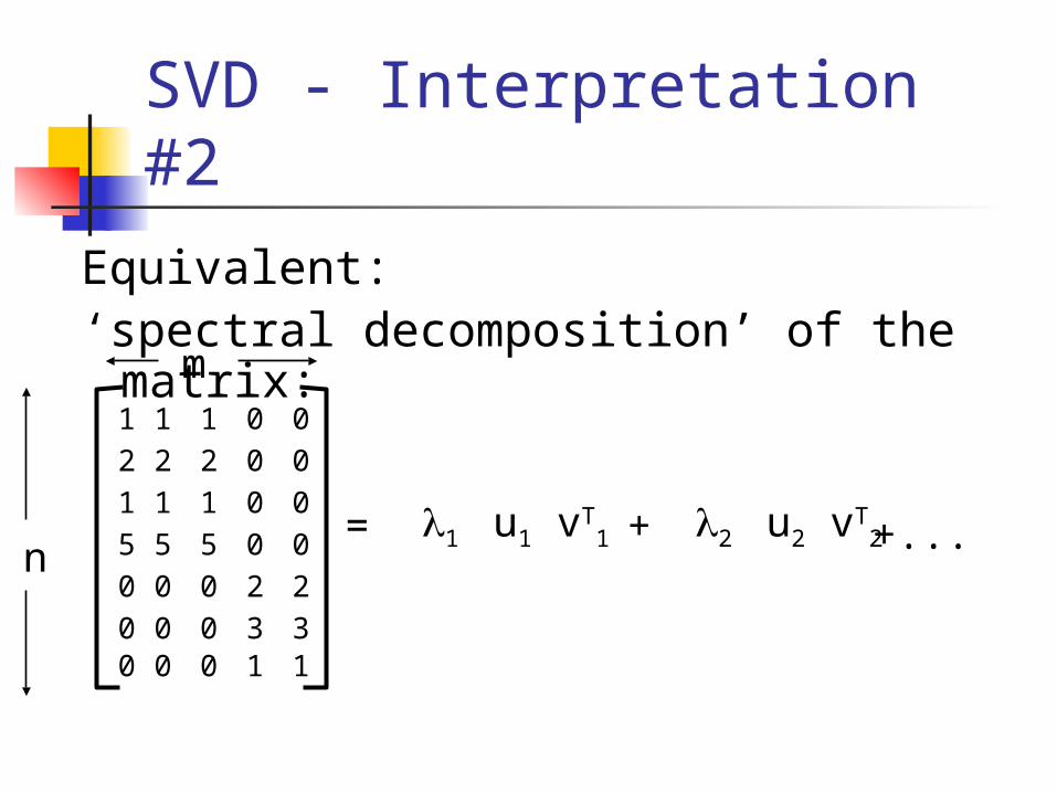
SVD - Interpretation #2

Equivalent:‘spectral decomposition’ of the

matrix:1 1 1 0 0

2 2 2 0 0

1 1 1 0 0

5 5 5 0 0

0 0 0 2 2

0 0 0 3 30 0 0 1 1

0.18 0

0.36 0

0.18 0

0.90 0

0 0.53

0 0.800 0.27

=9.64 0

0 5.29x

0.58 0.58 0.58 0 0

0 0 0 0.71 0.71

x

SVD - Interpretation #2

Equivalent:‘spectral decomposition’ of the

matrix:1 1 1 0 0

2 2 2 0 0

1 1 1 0 0

5 5 5 0 0

0 0 0 2 2

0 0 0 3 30 0 0 1 1

= x xu1 u2

1

2

v1

v2

SVD - Interpretation #2

Equivalent:‘spectral decomposition’ of the

matrix:1 1 1 0 0

2 2 2 0 0

1 1 1 0 0

5 5 5 0 0

0 0 0 2 2

0 0 0 3 30 0 0 1 1

= u11 vT1 u22 vT

2+ +...n

m

SVD - Interpretation #2

‘spectral decomposition’ of the matrix:

1 1 1 0 0

2 2 2 0 0

1 1 1 0 0

5 5 5 0 0

0 0 0 2 2

0 0 0 3 30 0 0 1 1

= u11 vT1 u22 vT

2+ +...n

m

n x 1 1 x m

r terms

SVD - Interpretation #2

approximation / dim. reduction:by keeping the first few terms (Q: how

many?)1 1 1 0 0

2 2 2 0 0

1 1 1 0 0

5 5 5 0 0

0 0 0 2 2

0 0 0 3 30 0 0 1 1

= u11 vT1 u22 vT

2+ +...n

m

assume: 1 >= 2 >= ...

SVD - Interpretation #2

A (heuristic - [Fukunaga]): keep 80-90% of ‘energy’ (= sum of squares of i ’s)

1 1 1 0 0

2 2 2 0 0

1 1 1 0 0

5 5 5 0 0

0 0 0 2 2

0 0 0 3 30 0 0 1 1

= u11 vT1 u22 vT

2+ +...n

m

assume: 1 >= 2 >= ...

SVD - Interpretation #3

finds non-zero ‘blobs’ in a data matrix

1 1 1 0 0

2 2 2 0 0

1 1 1 0 0

5 5 5 0 0

0 0 0 2 2

0 0 0 3 30 0 0 1 1

0.18 0

0.36 0

0.18 0

0.90 0

0 0.53

0 0.800 0.27

=9.64 0

0 5.29x

0.58 0.58 0.58 0 0

0 0 0 0.71 0.71

x

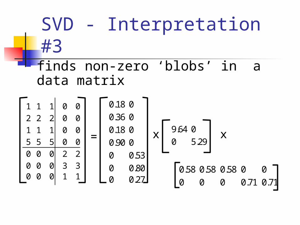
SVD - Interpretation #3 finds non-zero ‘blobs’ in a data

matrix

1 1 1 0 0

2 2 2 0 0

1 1 1 0 0

5 5 5 0 0

0 0 0 2 2

0 0 0 3 30 0 0 1 1

0.18 0

0.36 0

0.18 0

0.90 0

0 0.53

0 0.800 0.27

=9.64 0

0 5.29x

0.58 0.58 0.58 0 0

0 0 0 0.71 0.71

x

SVD - Interpretation #3 Drill: find the SVD, ‘by inspection’! Q: rank = ??

1 1 1 0 0

1 1 1 0 0

1 1 1 0 0

0 0 0 1 1

0 0 0 1 1

= x x?? ??

??

SVD - Interpretation #3 A: rank = 2 (2 linearly independent

rows/cols)

1 1 1 0 0

1 1 1 0 0

1 1 1 0 0

0 0 0 1 1

0 0 0 1 1

= x x??

??

?? 0

0 ??

??

??

SVD - Interpretation #3 A: rank = 2 (2 linearly independent

rows/cols)

1 1 1 0 0

1 1 1 0 0

1 1 1 0 0

0 0 0 1 1

0 0 0 1 1

= x x?? 0

0 ??

1 0

1 0

1 0

0 1

0 11 1 1 0 0

0 0 0 1 1

orthogonal??

SVD - Interpretation #3 column vectors: are orthogonal -

but not unit vectors:

1 1 1 0 0

1 1 1 0 0

1 1 1 0 0

0 0 0 1 1

0 0 0 1 1

= x x?? 0

0 ??

1/sqrt(3) 0

1/sqrt(3) 0

1/sqrt(3) 0

0 1/sqrt(2)

0 1/sqrt(2)

1/sqrt(3) 1/sqrt(3) 1/sqrt(3) 0 0

0 0 0 1/sqrt(2) 1/sqrt(2)

SVD - Interpretation #3 and the eigenvalues are:

1 1 1 0 0

1 1 1 0 0

1 1 1 0 0

0 0 0 1 1

0 0 0 1 1

= x x3 0

0 2

1/sqrt(3) 0

1/sqrt(3) 0

1/sqrt(3) 0

0 1/sqrt(2)

0 1/sqrt(2)

1/sqrt(3) 1/sqrt(3) 1/sqrt(3) 0 0

0 0 0 1/sqrt(2) 1/sqrt(2)

SVD - Interpretation #3 Q: How to check we are correct?

1 1 1 0 0

1 1 1 0 0

1 1 1 0 0

0 0 0 1 1

0 0 0 1 1

= x x3 0

0 2

1/sqrt(3) 0

1/sqrt(3) 0

1/sqrt(3) 0

0 1/sqrt(2)

0 1/sqrt(2)

1/sqrt(3) 1/sqrt(3) 1/sqrt(3) 0 0

0 0 0 1/sqrt(2) 1/sqrt(2)

SVD - Interpretation #3 A: SVD properties:

matrix product should give back matrix A

matrix U should be column-orthonormal, i.e., columns should be unit vectors, orthogonal to each other

ditto for matrix V matrix should be diagonal, with

positive values

SVD - Detailed outline Motivation Definition - properties Interpretation Complexity Case studies Additional properties

SVD - Complexity O( n * m * m) or O( n * n * m)

(whichever is less) less work, if we just want

eigenvalues or if we want first k eigenvectors or if the matrix is sparse [Berry] Implemented: in any linear algebra

package (LINPACK, matlab, Splus, mathematica ...)

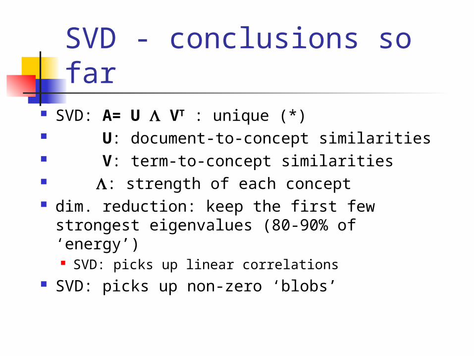
SVD - conclusions so far SVD: A= U VT : unique (*) U: document-to-concept similarities V: term-to-concept similarities : strength of each concept dim. reduction: keep the first few

strongest eigenvalues (80-90% of ‘energy’) SVD: picks up linear correlations

SVD: picks up non-zero ‘blobs’

References

Berry, Michael: http://www.cs.utk.edu/~lsi/ Fukunaga, K. (1990). Introduction to Statistical

Pattern Recognition, Academic Press. Press, W. H., S. A. Teukolsky, et al. (1992).

Numerical Recipes in C, Cambridge University Press.