multipair two-way half-duplex relaying with … two-way half-duplex relaying with massive arrays and...
TRANSCRIPT

arX
iv:1
607.
0159
8v1
[cs.
IT]
6 Ju
l 201
6
Multipair Two-way Half-Duplex Relaying with
Massive Arrays and Imperfect CSI
Chuili Kong, Student Member, IEEE, Caijun Zhong,Senior Member, IEEE,
Michail Matthaiou,Senior Member, IEEE, Emil Bjornson,Member, IEEE, and
Zhaoyang Zhang,Member, IEEE
Abstract
We consider a two-way half-duplex relaying system where multiple pairs of single antenna users
exchange information assisted by a multi-antenna relay. Taking into account the practical constraint of
imperfect channel estimation, we study the achievable sum spectral efficiency of the amplify-and-forward
(AF) and decode-and-forward (DF) protocols, assuming thatthe relay employs simple maximum ratio
processing. We derive an exact closed-form expression for the sum spectral efficiency of the AF protocol
and a large-scale approximation for the sum spectral efficiency of the DF protocol when the number of
relay antennas,M , becomes sufficiently large. In addition, we study how the transmit power scales with
M to maintain a desired quality-of-service. In particular, our results show that by using a large number of
relay antennas, the transmit powers of the user, relay, and pilot symbol can be scaled down proportionally
to 1/Mα, 1/Mβ, and1/Mγ for certainα, β, andγ, respectively. This elegant power scaling law reveals a
fundamental tradeoff between the transmit powers of the user/relay and pilot symbol. Finally, capitalizing
on the new expressions for the sum spectral efficiency, novelpower allocation schemes are designed to
further improve the sum spectral efficiency.
Index Terms
Amplify-and-forward, decode-and-forward, geometric programming, massive MIMO, power scaling
law, two-way relaying.
C. Kong, C. Zhong and Z. Zhang are with the Institute of Information and Communication Engineering, Zhejiang University,China. C. Zhong is also affiliated with the National Mobile Communications Research Laboratory, Southeast University,Nanjing,China (email: [email protected]).
M. Matthaiou is with the School of Electronics, Electrical Engineering and Computer Science, Queen’s University Belfast,Belfast, BT3 9DT, U.K. (email: [email protected]).
E. Bjornson is with the Department of Electrical Engineering (ISY), Linkoping University, Linkoping, SE-581 83, Sweden(email: [email protected]).

1
I. INTRODUCTION
Relaying is a low-complexity and cost-effective means to extend network coverage and provide
spatial diversity, which has attracted a great deal of research attention from both academia and
industry [1]–[4]. Thus far, most practical relaying systems are assumed to operate in the half-duplex
mode where the relay does not transmit and receive signals simultaneously. Yet, such half-duplex
mechanism incurs a 50% spectral efficiency loss. To reduce this loss in spectral efficiency, two-
way relaying was proposed in [5]–[8], where the two communicating nodes perform bidirectional
simultaneous data transmission.
Multipair two-way relaying is a sophisticated generalization of single pair two-way relaying,
where multiple pairs of users simultaneously establish a communication link with the aid of
a single shared relay [9]–[11], hence substantially boosting the system spectral efficiency. The
major challenge is to properly handle the inter-pair interference from co-existing communication
pairs. Thus far, a number of advanced techniques have been introduced to mitigate inter-pair
interference, such as dirty-paper coding [12] and interference alignment [13]. Unfortunately, the
practical implementation of these techniques is in generalvery complex. On the other hand, the
massive multiple-input multiple-output (MIMO) paradigm has demonstrated superior interference
suppression capabilities, with very simple and low-complexity linear processing [14]–[16]. There-
fore, deploying large-scale antenna arrays in two-way relaying systems appears to be an extremely
promising solution for inter-pair interference mitigation.
Some initial works have studied the fundamental performance of such systems [9], [10], [17].
In particular, for the amplify-and-forward (AF) protocol,[10] investigated the achievable rates and
power scaling laws of maximum ratio (MR) and zero-forcing (ZF) processing schemes. Moreover,
[9] derived a closed-form approximation of the ergodic rateof the MR scheme, and addressed
the optimal user pair selection problem. However, one majorlimitation of the above works is
that perfect channel state information (CSI) is assumed. Since obtaining perfect CSI is very
challenging in the context of massive MIMO systems, it is important to look into the realistic
scenario with imperfect CSI. An early attempt was made in [17], where the authors studied the
sum rate performance of training-based AF systems utilizing the ZF scheme. Although the derived
results are useful for understanding the impact of imperfect CSI on the system performance, a

2
number of important questions remain to be addressed. For instance, the fundamental tradeoff
between the transmit powers of pilot, user, and the relay, and the performance analysis of alternative
relay processing schemes, e.g., the decode-and-forward (DF) protocol, remain largely overlooked.
Motivated by this, in the current work, we consider a multipair two-way relaying system taking
into account the channel estimation error, and present an in-depth analysis of the achievable
spectral efficiency and power scaling law of MR processing for both the AF and DF protocols.
Specifically, the main contributions of this paper are summarized as follows:
• We investigate a multipair two-way relaying system that employs MR processing with im-
perfect CSI, and then derive an exact spectral efficiency expression in closed-form for the
AF protocol and a large-scale approximation of the spectralefficiency for the DF protocol
whenM → ∞, whereM is the number of relay antennas. Based on our analysis and results,
a comprehensive performance comparison of the two protocols is conducted.
• We characterize the power scaling laws for both the AF and DF protocols, which generalize
the results presented in [1], [9], [10]. It turns out that there exists a fundamental trade-off
between the transmit powers of each user, pilot symbol and the relay; in other words, the same
spectral efficiency can be achieved with different combination of power scaling parameters,
which permits great flexibility in the design of practical systems. In addition, our theoretical
findings suggest that it is worthwhile to spend more power on the pilot sequence to improve
the CSI accuracy instead of just increasing the users’ and relay power.
• Finally, to improve the sum spectral efficiency, we study thepower allocation problem for
both the AF and DF protocols subject to a sum power constraint. Near optimum solutions
are obtained by solving a sequence of geometric programming(GP) problems. Our numer-
ical results suggest that the proposed power allocation strategies improve the sum spectral
efficiency by 34.8% and 89.2% whenM = 300, for the AF and DF protocols, respectively,
indicating that the spectral efficiency enhancement is moreprominent for the DF protocol.
In addition, for the special case where all users have the same transmit power, it turns out
that the users should decrease their transmit power when thenumber of user pairs becomes
large. On the other hand, the users should increase their transmit power when the number of
relay antennas increases or when the channel estimation accuracy improves.

3
The remainder of the paper is organized as follows: Section II introduces the multipair two-
way half-duplex relaying system model under consideration. Section III presents an exact spectral
efficiency in closed-form for the AF protocol, and two large-scale approximations of the spectral
efficiency for both protocols, with imperfect CSI, while Section IV studies the power scaling
laws of different system configurations. The power allocation problem is discussed in Section V.
Finally, Section VI provides some concluding remarks.
Notation: We use bold upper case letters to denote matrices, bold lower case letters to denote
vectors and lower case letters to denote scalars. Moreover,(·)H , (·)∗, (·)T , and (·)−1 represent
the conjugate transpose operator, the conjugate operator,the transpose operator, and the matrix
inverse, respectively. Also,|| · || is the Euclidian norm,|| · ||F denotes the Frobenius norm,| · | is the
absolute value, and[A]mn gives the(m,n)-th entry ofA. In addition,x ∼ CN (0,Σ) denotes a
circularly symmetric complex Gaussian random vectorx with zero mean and variance matrixΣ,
while Ik is the identity matrix of sizek. Finally, the statistical expectation operator is represented
by E{·}, the variance operator is Var(·), the trace is denoted by tr(·), and the notationa.s.→ means
almost sure convergence.
II. SYSTEM MODEL
Consider a multipair two-way relaying system as illustrated in Fig. 1, whereN pairs of single-
antenna users, denoted as TA,i and TB,i, i = 1, . . . , N , intend to exchange information with each
other, under the assistance of a shared relay TR equipped withM antennas. We assume that the
direct links between TA,i and TB,i do not exist due to large obstacles or severe shadowing [11].
Also, the relay operates in the half-duplex mode, i.e., it cannot transmit and receive simultaneously.
It is assumed that the system works under the time division duplex protocol and channel
reciprocity holds. As such, the uplink and downlink channels between TA,i and TR can be denoted
asgAR,i andgTAR,i, respectively. Similarly, the channels between TB,i and TR are denoted asgRB,i
andgTRB,i, i = 1, . . . , N , respectively, which account for both small-scale fading and large-scale
fading. More precisely,gAR,i ∼ CN (0, βAR,iIM) and gRB,i ∼ CN (0, βRB,iIM). This model
is known as uncorrelated Rayleigh fading, andβAR,i and βRB,i model the large-scale path-loss
effect, which are assumed to be constant over many coherenceintervals and known a priori.

4
M,1
TA
,TA i
,TA N
,1TB
,TB i
,TB N
TR
1
T
ARg
1ARg
,
T
AR ig
,AR ig
,
T
AR Ng
,AR Ng
1
T
RBg
1RBg
,
T
RB ig
,RB ig
,
T
RB Ng
,RB Ng
Fig. 1: Illustration of the multipair two-way relaying system.
For notational convenience, the channel vectors can be collected together in a matrix form as
GAR , [gAR,1, . . . , gAR,N ] ∈ CM×N andGRB , [gRB,1, . . . , gRB,N ] ∈ C
M×N .
For the considered multipair two-way relaying system, the entire information transmission
process consists of two separate phases. In the first phase, the N user pairs TA,i and TB,i
simultaneously transmit their respective signals to TR. Thus, the received signal at TR is given by
yr =N∑
i=1
(√pA,igAR,ixA,i +
√pB,igRB,ixB,i
)+ nR, (1)
wherexA,i andxB,i are Gaussian signals with zero mean and unit power transmitted by thei-th
user pair,pA,i and pB,i are the average transmit power of TA,i and TB,i, respectively, andnR is
a vector of additive white Gaussian noise (AWGN) at TR, whose elements are identically and
independently distributed (i.i.d.)CN (0, 1). Note that to keep the notation clean and without loss
of generality, we take the noise variance to be1 here, and also in the subsequent sections. With
this convention,pA,i andpB,i can be interpreted as the normalized transmit signal-to-noise (SNR).
In the second phase, the relay broadcasts a transformed version of the received signal to all
users. Depending on the adopted relaying protocol, two separate scenarios are studied.
1) AF protocol: With the AF protocol, the relay first implements a type of linear processing
on the received signal, and then forwards it to all users. Thus, the transmit signal from TR can

5
be written as
yAFt = ρAFFyr, (2)
whereF ∈ CM×M is the linear processing matrix to be specified shortly, andρAF is a normalization
coefficient, which is chosen to satisfy the long-term total transmit power constraint at the relay,
namely,E{||yAF
t ||2}= pr, so thatpr is the average transmit power of the relay.
Therefore, the received signals at TX,i (whereX ∈ {A,B}) is given by
zAFX,i = gT
XR,iyAFt + nX,i, (3)
where nX,i ∼ CN (0, 1) represents the AWGN at TX,i. Please note, to simplify notation, we
introducegBR,i which is defined asgBR,i , gRB,i due to the channel reciprocity.
2) DF protocol: With the DF protocol, the relay first decodes the2N symbols, and then re-
encodes and forwards the signals to all users. To reduce the complexity, single user linear detection
is considered at the relay. As such, the transformed signal after linear processing can be expressed
as
rDF = WTyr, (4)
whereWT ∈ C2N×M is the linear receiver matrix, which will be specified shortly.
After decoding the2N symbolsx from rDF, the remaining task is broadcasting, but before
this, a linear precoding matrixJ ∈ CM×2N is applied to the re-generated symbols. As such, the
transmit signal of TR is given by
yDFt = ρDFJx, (5)
wherex =[xTA,x
TB
]Twith xA = [xA,1, . . . , xA,N ]
T andxB = [xB,1, . . . , xB,N ]T , andρDF is the
normalization coefficient, which is determined by the average power constraint at the relay, i.e.,
E
{||yDF
t ||2}= pr. Hence, the signals received at TX,i can be expressed as
zDFX,i = gT
XR,iyDFt + nX,i. (6)

6
A. Channel Estimation
In practice, the channelsGAR andGRB are not known and need to be estimated at the relay in
every coherence interval. The typical way of doing this is toutilize pilots [14]. To this end, during
each coherence interval of lengthτc (in symbols),τp symbols are used for channel training. In
this case, TA,i and TB,i transmit simultaneously their mutually orthogonal pilot sequences to TR,
for i = 1, . . . , N . Thus, the received pilot matrix at the relay is given by
Yp =√τpppGARΦ
TA +
√τpppGRBΦ
TB +Np, (7)
wherepp is the transmit power of each pilot symbol,Np is AWGN matrix including i.i.d.CN (0, 1)
elements, while thei-th columns ofΦA ∈ Cτp×N and ΦB ∈ Cτp×N are the pilot sequences
transmitted from TA,i and TB,i, respectively. Since all pilot sequences are assumed to be mutually
orthogonal,τp ≥ 2N is required, and we have thatΦTAΦ
∗A = IN , ΦT
BΦ∗B = IN , andΦT
AΦ∗B = 0N .
As in [1], [17], [18], we assume that TR uses the minimum mean-square-error (MMSE) estimator
to estimateGAR andGRB. As such, the estimated channels ofGAR andGRB are given by
GAR =1
√τppp
YpΦ∗ADAR =
(
GAR +1
√τppp
NA
)
DAR, (8)
GRB =1
√τppp
YpΦ∗BDRB =
(
GRB +1
√τppp
NB
)
DRB, (9)
respectively, whereDAR ,
(1
τpppD−1
AR + IN
)−1
with [DAR]ii = βAR,i (DAR is anN×N diagonal
matrix), DRB ,
(1
τpppD−1
RB + IN
)−1
with [DRB]ii = βRB,i (DRB is anN ×N diagonal matrix),
NA , NpΦ∗A, andNB , NpΦ
∗B. SinceΦT
AΦ∗A = IN andΦT
BΦ∗B = IN , the elements ofNA and
NB are i.i.d.CN (0, 1) random variables. LetEAR andERB be the estimation error matrices of
GAR andGRB, respectively. Then,GAR andGRB can be decomposed as
GAR = GAR + EAR, (10)
GRB = GRB + ERB, (11)
respectively. Due to the orthogonality property of MMSE estimators and the fact thatGAR, EAR,
GRB , andERB are complex Gaussian distributed, these matrices are independent of each other.

7
By rewriting (10) in vector form, we have
gAR,i = gAR,i + eAR,i, (12)
gRB,i = gRB,i + eRB,i, (13)
wheregAR,i, eAR,i, gRB,i, andeRB,i are thei-th columns ofGAR, EAR, GRB, andERB, respec-
tively, which are mutually independent. Then, from (8), theelements ofgAR,i, eAR,i are Gaussian
random variables with zero mean, varianceσ2AR,i andσ2
AR,i, respectively, whereσ2AR,i ,
τpppβ2AR,i
1+τpppβAR,i
andσ2AR,i ,
βAR,i
1+τpppβAR,i. Similarly, the elements ofgRB,i, andeRB,i are complex Gaussian random
variables with zero mean, varianceσ2RB,i and σ2
RB,i, respectively, whereσ2RB,i ,
τpppβ2RB,i
1+τpppβRB,iand
σ2RB,i ,
βRB,i
1+τpppβRB,i.
B. Linear Processing Matrices
The relay TR treats the channel estimates as the true channels and utilizes them to perform
linear processing. For both the AF and DF protocols, the MR linear processing method is used.1
1) AF protocol: With MR, the processing matrixF ∈ CM×M is given by [9]
F = B∗AH , (14)
whereA ,
[
GAR, GRB
]
, B ,
[
GRB, GAR
]
. Recall thatρAF satisfies the long-term total transmit
power constraint at the relay, and after some simple algebraic manipulations, we have
ρAF =
√√√√√
prN∑
i=1
(pA,iE {||FgAR,i||2}+ pB,iE {||FgRB,i||2}) + E {||F||2F}. (15)
2) DF protocol: With MR, the processing matrixWT ∈ C2N×M andJ ∈ CM×2N are given by
WT =[
GAR, GRB
]H
, (16)
J =[
GRB , GAR
]∗
, (17)
1Note that MR is a very attractive linear processing technique in the context of massive MIMO systems due to its low complexity.Most importantly, it can be implemented in a distributed manner [14], [15].

8
respectively, whileρDF is given by
ρDF =
√pr
E {||J||2F}=
√√√√√
pr
MN∑
n=1
(σ2AR,n + σ2
RB,n
). (18)
III. SPECTRAL EFFICIENCY
In this section, we investigate the spectral efficiency (in bit/s/Hz) of the two-way half-duplex
relaying system. In particular, for the AF protocol, an exact spectral efficiency expression in
closed-form is derived for arbitraryM . Furthermore, two large-scale approximations of the spectral
efficiency for both protocols are deduced whenM → ∞.
A. AF protocol
Without loss of generality, we focus on the characterization of the achievable spectral effi-
ciency of user TA,i. With the AF protocol, when TA,i receives the superimposed signal from
TR, it first makes an attempt to subtract its own transmitted message according to its available
CSI (known as self-interference cancellation). In the current work, we consider the realistic
case where the users do not have access to instantaneous CSI,hence TA,i uses only statisti-
cal CSI to cancel the self-interference. Therefore, after cancelling partial self-interference, i.e.,
ρAF√pA,iE
{gTAR,iFgAR,i
}xA,i, the received signal at TA,i can be re-expressed as
zAFA,i = zAF
A,i − ρAF√pA,iE
{gTAR,iFgAR,i
}xA,i (19)
= ρAF√pB,iE
{gTAR,iFgRB,i
}xB,i
︸ ︷︷ ︸
desired signal
+ ρAF√pB,i
(gTAR,iFgRB,i − E
{gTAR,iFgRB,i
})xB,i
︸ ︷︷ ︸
estimation error
(20)
+ ρAF√pA,i
(gTAR,iFgAR,i − E
{gTAR,iFgAR,i
})xA,i
︸ ︷︷ ︸
residual self-interference
(21)
+ ρAF
∑
j 6=i
(√pA,ig
TAR,iFgAR,jxA,j +
√pB,ig
TAR,iFgRB,jxB,j
)
︸ ︷︷ ︸
inter-user interference
+ ρAFgTAR,iFnR + nA,i
︸ ︷︷ ︸
compound noise
. (22)
Note that, TA,i tries to utilize the statistical informationE{gTAR,iFgAR,i
}to cancel partial

9
interference. Focusing on this, we have
E
{gTAR,iFgAR,i
}= E
{N∑
n=1
(gTAR,ig
∗RB,ng
HAR,ngAR,i + gT
AR,ig∗AR,ng
HRB,ngAR,i
)
}
, (23)
= E
{gTAR,ig
∗RB,ig
HAR,igAR,i + gT
AR,ig∗AR,ig
HRB,igAR,i
}= 0, (24)
which indicates that no effective self-interference cancellation can be achieved by TA,i if only
statistical CSI is available. In sharp contrast, if TA,i knows perfect or estimated CSI, it is ca-
pable of completely canceling the self-interference [9], or ρAF√pA,ig
TAR,iFgAR,ixA,i [19], [20],
respectively. Nevertheless, the overhead associated withCSI acquisition at users may overweigh
the performance gains brought by effective self-interference cancellation, particularly in massive
MIMO systems.
Using a standard approach as in [1], [21], an ergodic achievable spectral efficiency of TA,i is
RAFA,i =
1
2log2
(
1 +AAF
i
BAFi + CAF
i +DAFi + EAF
i
)
, (25)
where
AAFi = pB,i|E
{gTAR,iFgRB,i
}|2, (26)
BAFi = pB,iVar
(gTAR,iFgRB,i
), (27)
CAFi = pA,iVar
(gTAR,iFgAR,i
), (28)
DAFi =
∑
j 6=i
(E
{pA,i|gT
AR,iFgAR,j |2 + pB,i|gTAR,iFgRB,j |2
}), (29)
EAFi = E
{||gT
AR,iF||2}+
1
ρ2AF
. (30)
Thus, the ergodic sum spectral efficiency of the multipair two-way AF relaying system is given
by
RAF =τc − τp
τc
N∑
i=1
(RAF
A,i +RAFB,i
), (31)
whereRAFB,i is the spectral efficiency of TB,i, which can be derived in a similar fashion.
In the following, we present an exact analysis of the spectral efficiency based on (25).
Theorem 1: With the AF protocol, the ergodic spectral efficiencyRAFA,i for an arbitrary number

10
of relay antennas is given by (25) with
AAFi = pB,iM
2(M + 1)2σ4AR,iσ
4RB,i, (32)
BAFi = pB,i2M (M + 1)βAR,iβRB,i
N∑
n=1
σ2AR,nσ
2RB,n (33)
+ pB,iM (M + 1)σ2AR,iσ
2RB,i
(βAR,iσ
2RB,i + βRB,iσ
2AR,i
)+ pB,iM
2σ2AR,iσ
2RB,iσ
2AR,iσ
2RB,i
+ pB,i2M (M + 1)2 σ4AR,iσ
4RB,i + pB,i2M (M + 1)σ4
AR,iσ2AR,iσ
2RB,i + pB,i2M (M + 1)σ2
AR,iσ2AR,iσ
4RB,i
+ pB,i2Mσ2AR,iσ
2AR,iσ
2RB,iσ
2RB,i + pB,iM
2 (M + 1)σ4AR,iσ
2AR,iσ
2RB,i
+ pB,iM2 (M + 1) σ2
AR,iσ2AR,iσ
4RB,i + pB,iM
2σ2AR,iσ
2AR,iσ
2RB,iσ
2RB,i,
CAFi = 4pA,iM(M + 1)β2
AR,i
N∑
n=1
σ2AR,nσ
2RB,n (34)
+ 4pA,iσ2AR,iσ
2RB,iM (M + 1)
((M + 2)σ4
AR,i + (M + 5)σ2AR,iσ
2AR,i + σ4
AR,i
),
DAFi =
∑
j 6=i
2M (M + 1)βAR,i (pA,iβAR,j + pB,iβRB,j)∑
n 6=i,j
σ2AR,nσ
2RB,n (35)
+∑
j 6=i
Mσ2AR,iσ
2RB,i (pA,iβAR,j + pB,iβRB,j)
((M + 1) (M + 3) σ2
AR,i + 2 (M + 1) σ2AR,i
)
+∑
j 6=i
MβAR,iσ2AR,jσ
2RB,j
((M + 1) (M + 3)
(pA,iσ
2AR,j + pB,iσ
2RB,j
)+ 2 (M + 1)
(pA,iσ
2AR,j + pB,iσ
2RB,j
)),
EAFi = 2M (M + 1)βAR,i
∑
n 6=i
σ2AR,nσ
2RB,n (36)
+Mσ2AR,iσ
2RB,i
((M + 1) (M + 3) σ2
AR,i + 2 (M + 1) σ2AR,i
)
+1
pr
N∑
i=1
Mσ2AR,iσ
2RB,i
((M + 1) (M + 3)
(σ2AR,ipA,i + σ2
RB,ipB,i
)+ 2 (M + 1)
(σ2AR,ipA,i + σ2
RB,ipB,i
))
+1
pr
N∑
i=1
2M (M + 1) (βAR,ipA,i + βRB,ipB,i)∑
n 6=i
σ2AR,nσ
2RB,n +
1
pr2M (M + 1)
N∑
n=1
σ2AR,n.σ
2RB,n.
Proof: See Appendix I. �
Theorem 1 presents an exact spectral efficiency in closed-form, which is applicable to arbitrary
system configurations. However, the expression is too complicated to provide useful insights.
Using the fact that the relay is equipped with a massive antenna array, we now obtain a simple
and accurate approximation for the spectral efficiency.
Theorem 2: With the AF protocol, as the number of relay antennas grows toinfinity, then we
11
haveRAFA,i − RAF
A,i
M→∞−→ 0, whereRAFA,i is given by
RAFA,i ,
1
2log2
(
1 +pB,iM
BAFi + CAF
i + DAFi + EAF
i
)
, (37)
where
BAFi , pB,i
(
βRB,i
σ2RB,i
+βAR,i
σ2AR,i
)
, (38)
CAFi ,
4pA,iβAR,i
σ2RB,i
, (39)
DAFi ,
∑
j 6=i
pA,j
(
βAR,j
σ2RB,i
+σ4AR,jσ
2RB,jβAR,i
σ4AR,iσ
4RB,i
)
+∑
j 6=i
pB,j
(
βRB,j
σ2RB,i
+σ2AR,jσ
4RB,jβAR,i
σ4AR,iσ
4RB,i
)
, (40)
EAFi ,
1
σ2RB,i
+1
prσ4AR,iσ
4RB,i
N∑
n=1
σ2AR,nσ
2RB,n
(pA,nσ
2AR,n + pB,nσ
2RB,n
). (41)
Proof: WhenM is infinitely large, the lower order terms in (32), (33), (34), (35), and (36)
are trivial. Thus, by removing them and keeping only the highest order terms, we complete the
proof. �
Theorem 2 presents a large-scale approximation of thei-th user’s spectral efficiency. Despite
being obtained under the massive array assumption, the approximation turns out to be very accurate
even for finite number of relay antennas. In addition, it is easy to observe the impact of various
factors on the spectral efficiency. For instance,BAFi represents the influence of the estimation
error, Ci denotes the residual self-interference,DAFi stands for the inter-user interference caused
by other user pairs, andEAFi is composed of the SNR at the relay and the end TA,i.
From Theorem 2, we observe thatRAFA,i is an increasing function with respect toM , while a
decreasing function with respect toBAFi , CAF
i , DAFi , and EAF
i . Also, focusing on the termDAFi ,
it can be seen that the individual user spectral efficiencyRAFA,i decreases with the number of user
pairs N ; this is anticipated since a higher number of users increases the amount of inter-user
interference. Now, we focus on studying the impact of the transmit power ofi-th user pairpA,i
and pB,i, the transmit power of the relaypr, and the transmit power of each pilot symbolpp on
the system performance. As can be seen, whenpA,i → ∞ andpB,i → ∞, the spectral efficiency
is limited by pr andpp; in contrast, it is limited bypA,i, pB,i, andpp whenpr → ∞. Moreover,
when pA,i → ∞, pB,i → ∞, andpr → ∞, EAFi → 0, which indicates that the noise at the relay

12
and TA,i can be neglected when the transmit powers of each user and therelay are large enough.
B. DF protocol
With the DF protocol, in the first phase, a linear processing matrix WT is applied to the received
signals prior to signal detection, hence, the post-processing signals at the relay are given by
rDF =
N∑
i=1
(√pA,iG
HARgAR,ixA,i +
√pB,iG
HARgRB,ixB,i
)
+ GHARnR
N∑
i=1
(√pA,iG
HRBgAR,ixA,i +
√pB,iG
HRBgRB,ixB,i
)
+ GHRBnR
, (42)
where the topN elements ofrDF stand for the signals from TA,i (i = 1, . . . , N), while the bottom
N elements ofrDF represent the signals from TB,i (i = 1, . . . , N). Without loss of generality, we
focus only on thei-th pair of users, i.e., TA,i and TB,i. This is a superposition of thei-th and
(N+i)-th elements ofrDF, and can be expressed as
rDFi = rDF
i + rDFN+i, (43)
=N∑
j=1
(√pA,j
(gHAR,igAR,j + gH
RB,igAR,j
)xA,j +
√pB,j
(gHAR,igRB,j + gH
RB,igRB,j
)xB,j
)(44)
+(gHAR,i + gH
RB,i
)nR, (45)
=√pA,i
(gHAR,igAR,i + gH
RB,igAR,i
)xA,i +
√pB,i
(gHAR,igRB,i + gH
RB,igRB,i
)xB,i
︸ ︷︷ ︸
desired signal
(46)
+√pA,i
(gHAR,ieAR,i + gH
RB,ieAR,i
)xA,i +
√pB,i
(gHAR,ieRB,i + gH
RB,ieRB,i
)xB,i
︸ ︷︷ ︸
estimation error
(47)
+∑
j 6=i
(√pA,j
(gHAR,igAR,j + gH
RB,igAR,j
)xA,j +
√pB,j
(gHAR,igRB,j + gH
RB,igRB,j
)xB,j
)
︸ ︷︷ ︸
inter-user interference
(48)
+(gHAR,i + gH
RB,i
)nR
︸ ︷︷ ︸
compound noise
. (49)
Since the relay has estimated CSI, it treats the channel estimates as the true channels to decode
the signals. To this end, using a standard bound based on the worst-case uncorrelated additive

13
noise [21] yields the ergodic spectral efficiency of thei-th user pair in the first phase
RDF1,i =
1
2E
log2
1 +ADF
i +BDFi
E
{
(CDFi +DDF
i + EDFi ) |GAR, GRB
}
, (50)
where the inner and outer expectations are taken over the estimation errors and channel estimates,
respectively, and
ADFi = pA,i
(|gH
AR,igAR,i|2 + |gHRB,igAR,i|2
), (51)
BDFi = pB,i
(|gH
AR,igRB,i|2 + |gHRB,igRB,i|2
), (52)
CDFi = pA,i
(|gH
AR,ieAR,i|2 + |gHRB,ieAR,i|2
)+ pB,i
(|gH
AR,ieRB,i|2 + |gHRB,ieRB,i|2
), (53)
DDFi =
∑
j 6=i
(pA,j
(|gH
AR,igAR,j |2 + |gHRB,igAR,j|2
)+ pB,j
(|gH
AR,igRB,j |2 + |gHRB,igRB,j |2
)), (54)
EDFi = ||gAR,i||2 + ||gRB,i||2. (55)
In addition, the ergodic spectral efficiency of the TX,i → TR (X ∈ {A,B}) link can be obtained
as
RDFXR,i =
1
2E
log2
1 +XDF
i
E
{
(CDFi +DDF
i + EDFi ) |GAR, GRB
}
. (56)
In the second phase, the relay broadcasts to all users using the MR principle; hence the received
signal at TX,i is given by
zDFX,i = ρDF
N∑
j=1
(gTXR,ig
∗RB,jxA,j + gT
XR,ig∗AR,jxB,j
)+ nX,i. (57)
Similar to the AF protocol, partial self-interference cancellation according to the statistical
knowledge of the channel gains can be performed at TA,i and TB,i after receiving the superimposed

14
signal from TR. Thus the post-processing signals at TA,i and TB,i can be re-expressed as,
zDFA,i = zDF
A,i − ρDFE{gTAR,ig
∗RB,i
}xA,i (58)
= ρDFE{gTAR,ig
∗AR,i
}xB,i
︸ ︷︷ ︸
desired signal
+ ρDF
(gTAR,ig
∗AR,i − E
{gTAR,ig
∗AR,i
})xB,i
︸ ︷︷ ︸
estimation error
(59)
+ ρDF
(gTAR,ig
∗RB,i − E
{gTAR,ig
∗RB,i
})xA,i
︸ ︷︷ ︸
residual self-interference
(60)
+ ρDF
∑
j 6=i
(gTAR,ig
∗RB,jxA,j + gT
AR,ig∗AR,jxB,j
)
︸ ︷︷ ︸
inter-user interference
+ nA,i︸︷︷︸
noise
. (61)
zDFB,i = zDF
B,i − ρDFE{gTRB,ig
∗AR,i
}xB,i (62)
= ρDFE{gTRB,ig
∗RB,i
}xA,i
︸ ︷︷ ︸
desired signal
+ ρDF
(gTRB,ig
∗RB,i − E
{gTRB,ig
∗RB,i
})xA,i
︸ ︷︷ ︸
estimation error
(63)
+ ρDF
(gTRB,ig
∗AR,i − E
{gTRB,ig
∗AR,i
})xB,i
︸ ︷︷ ︸
residual self-interference
(64)
+ ρDF
∑
j 6=i
(gTRB,ig
∗RB,jxA,j + gT
RB,ig∗AR,jxB,j
)
︸ ︷︷ ︸
inter-user interference
+ nB,i︸︷︷︸
noise
. (65)
Therefore, the ergodic spectral efficiency of the TR → TX,i link is expressed as
RDFRX,i =
1
2log2
(1 + SINRDF
RX,i
), (66)
where
SINRDFRX,i =
|E{gTXR,ig
∗XR,i
}|2
Var(gTXR,ig
∗XR,i
)+ Var
(gTAR,ig
∗RB,i
)+∑
j 6=i
(E
{|gT
XR,ig∗RB,j |2
}+ E
{|gT
XR,ig∗AR,j|2
})+ 1
ρ2DF
.
(67)
Now, according to [22]–[27], the ergodic spectral efficiency of thei-th user pair can be expressed
as
RDFi = min
(RDF
1,i , RDF2,i
), (68)

15
where
RDF2,i = min
(RDF
AR,i, RDFRB,i
)+ min
(RDF
BR,i, RDFRA,i
)(69)
Thus, the ergodic sum spectral efficiency of the multipair two-way DF relaying system is given
by
RDF =τc − τp
τc
N∑
i=1
RDFi . (70)
When TR employs a very large antenna array, i.e.,M → ∞, the large-scale approximation of
the spectral efficiency of thei-th user pair is presented in the following theorem.
Theorem 3: With the DF protocol, as the number of relay antennas grows toinfinity, then we
haveRDFi − RDF
i
M→∞−→ 0 , whereRDFi is given by
RDFi , min
(
RDF1,i , R
DF2,i
)
, (71)
with
RDF1,i ,
1
2log2
1 +pA,i
(Mσ4
AR,i + σ2AR,iσ
2RB,i
)+ pB,i
(Mσ4
RB,i + σ2AR,iσ
2RB,i
)
(σ2AR,i + σ2
RB,i
)
(
pA,iσ2AR,i + pB,iσ2
RB,i +∑
j 6=i
(pA,jβAR,j + pB,jβRB,j) + 1
)
,
(72)
RDF2,i , min
(
RDFAR,i, R
DFRB,i
)
+ min(
RDFBR,i, R
DFRA,i
)
, (73)
where
RDFAR,i ,
1
2log2
1 +pA,i
(Mσ4
AR,i + σ2AR,iσ
2RB,i
)
(σ2AR,i + σ2
RB,i
)
(
pA,iσ2AR,i + pB,iσ2
RB,i +∑
j 6=i
(pA,jβAR,j + pB,jβRB,j) + 1
)
,
(74)
RDFRA,i ,
1
2log2
1 +
prMσ4AR,i
(prβAR,i + 1)N∑
j=1
(σ2AR,j + σ2
RB,j
)
, (75)

16
and RDFBR,i and RDF
RB,i are obtained by replacing the transmit powerspA,i, pB,i, and the subscripts
“AR”, “RB” with the transmit powerspB,i, pA,i, and the subscripts “RB”, “AR” inRDFAR,i and
RDFRA,i, respectively.
Proof: See Appendix II. �
Theorem 3 provides a large-scale approximation of thei-th user pair’s spectral efficiency. More
specifically, RDF1,i , R
DFAR,i, and RDF
BR,i are computed by utilizing the law of large numbers, while
RDFRA,i and RDF
RB,i are the exact expressions forRDFRA,i and RDF
RB,i. From this approximation, we
can see thatRDFi is an increasing function with respect topA,i, pB,i, and pr. However, when
pA,i → ∞, pB,i → ∞, and/orpr → ∞, RDFi converges to a non-zero limit, due to strong inter-user
interference. Moreover, we observe thatRDFi increases with the number of relay antennasM ,
indicating the strong advantage of employing massive antenna arrays at the relay, while decreases
with the number of user pairsN , which is expected since larger number of users increases the
amount of inter-user interference. Finally, whenpr → 0 the bottleneck of spectral efficiency occurs
in the second phase, while the opposite holds whenpA,i → 0 andpB,i → 0, where we have
RDFi − 1
2log2
(
1 +pA,iσ
2AR,i
(Mσ2
AR,i + σ2RB,i
)+ pB,iσ
2RB,i
(σ2AR,i +Mσ2
RB,i
)
σ2AR,i + σ2
RB,i
)
→ 0.
It is of interest to compare the achievable sum rates of AF andDF protocols in the lowpA,i and
pB,i regime for massive MIMO systems which have the potential to save an order of magnitude
in transmit power. Then, we have the following corollary.
Corollary 1: In the low SNR regime, i.e.,pA,i → 0 andpB,i → 0, we haveRAFA,i+ RAF
B,i > RDFi .
Proof: WhenpA,i → 0 andpB,i → 0, we have
RAFA,i −
1
2log2
(1 + pB,iMσ2
RB,i
)→ 0, (76)
RAFB,i −
1
2log2
(1 + pA,iMσ2
AR,i
)→ 0. (77)

17
To this end, it can be shown that
1 +pA,iσ
2AR,i
(Mσ2
AR,i + σ2RB,i
)+ pB,iσ
2RB,i
(σ2AR,i +Mσ2
RB,i
)
σ2AR,i + σ2
RB,i
, (78)
< 1 +pA,iσ
2AR,iM
(σ2AR,i + σ2
RB,i
)+ pB,iσ
2RB,iM
(σ2AR,i + σ2
RB,i
)
σ2AR,i + σ2
RB,i
, (79)
= 1 + pA,iMσ2AR,i + pB,iMσ2
RB,i, (80)
<(1 + pA,iMσ2
AR,i
) (1 + pB,iMσ2
RB,i
), (81)
which completes the proof. �
Corollary 1 indicates that the AF protocol outperforms the DF protocol in the low SNR regime.
C. Numerical Results
We now present numerical results to validate the above analytical results. For all illustrative
examples, the following set of parameters are used in simulation. The length of the coherence
interval is τc = 196 (symbols), chosen by the LTE standard. The length of the pilot sequences
is τp = 2N which is the minimum requirement. For simplicity, we set thelarge-scale fading
coefficientβAR = βRB = 1, and assume that each user has the same transmit power, i.e.,pA,i =
pB,i = pu.
1) Validation of analytical expressions: We assume thatpp = pu, and that the total transmit
power of theN user pairs is equal to the transmit power of the relay, i.e.,pr = 2Npu.
Fig. 2 shows the sum spectral efficiency versus the transmit power of each userpu for different
number of relay antennas. Note that the “Approximations” curves are obtained by using (37) and
(71), and the “Numerical results” curves are generated by Monte-Carlo simulation according to
(31) and (70) by averaging over104 independent channel realizations, for the AF and DF proto-
cols, respectively. As can be readily observed, the large-scale approximations are very accurate,
especially for large antenna arrays. Moreover, we can see that increasing the number of relay
antennas significantly yields higher spectral efficiency, as expected.
2) Comparison of the AF and DF protocols: We now compare the sum spectral efficiency of
the AF and DF protocols for different system configurations,i.e., different transmit powerspu,
pr, andpp, and different number of relay antennasM and user pairsN .

18
−20 −15 −10 −5 0 5 10 15 200
2
4
6
8
10
12
14
16
pu (dB)
Sum
spe
ctra
l effi
cien
cy (
bit/s
/Hz)
Numerical results−AFApproximations−AFNumerical results−DFApproximations−DF
M = 50
M = 200
Fig. 2: Sum spectral efficiency versuspu for N = 5, pp = pu andpr = 2Npu.
−30 −25 −20 −15 −10 −5 0 5 100
1
2
3
4
5
6
pu (dB)
Sum
spe
ctra
l effi
cien
cy (
bit/s
/Hz)
AFDF
M = 100, N = 5
M = 150, N = 5
M = 150, N = 40
Fig. 3: Spectral efficiency versuspu for pr = −10 dB andpp = 10 dB.
Fig. 3 shows the sum spectral efficiency versus the transmit power of each userpu for different
M andN with pr = −10 dB andpp = 10 dB. We can observe that for smallpu, the AF protocol
outperforms the DF protocol, which is consistent with the result in Corollary 1. The reason is
that whenpu is small, the spectral efficiency of the DF protocol is limited by the performance
in the first phase. On the other hand, whenpu is large, the noise amplification phenomenon of
the AF protocol will significantly affect the spectral efficiency of the relay to the destination link;
this makes DF outperform the AF protocol by eliminating the noise and preventing interference
accumulation at the end users.
Fig. 4 provides the sum spectral efficiency versus the transmit power of the relaypr for different

19
−20 −15 −10 −5 0 5 10 15 200
5
10
15
20
25
30
35
40
pr (dB)
Sum
spe
ctra
l effi
cien
cy (
bit/s
/Hz)
AFDF
M = 100, N = 30
M = 300, N = 30
M = 100, N = 5
Fig. 4: Sum spectral efficiency versus the transmit power of the relaypr for pu = 10 dB andpp = 10 dB.
M andN with pu = 10 dB andpp = 10 dB. As we can observe, the DF protocol is superior to
the AF protocol in the lowpr regime but becomes inferior in the highpr regime. This is due to
the fact that lowpr makes the AF protocol suffer severe noise amplification effect and thus leads
to spectral efficiency reduction. In addition, focusing on the particular operating pointpr = 0 dB,
we see that the DF protocol achieves higher sum spectral efficiency whenM = 100 andN = 30,
while the AF protocol becomes better whenM = 300 andN = 30 or M = 100 andN = 30. The
reason is that the residual interference due to inaccurate channel estimation is a key performance
limiting factor for the AF protocol; in other words, the larger theN , the stronger the interference.
As such, less user pairs are preferable for the AF protocol. However, it turns out that increasing
the number of relay antennas is an effective way to mitigate such a detrimental effect.
Fig. 5 presents the sum spectral efficiency versus the transmit power of each pilot symbolpp
for differentM andN with pu = 0 dB andpr = 0 dB. Similarly, we observe that for fixedN = 5
andM , the DF protocol outperforms the AF protocol in the lowpp regime while the converse
holds in the highpp regime. In addition, focusing on the curves associated withM = 300 and
N = 50, we see that the spectral efficiency of the DF protocol is higher than that of the AF
protocol, indicating that a largeN is preferred for the DF protocol.
Fig. 6 illustrates the impact of number of user pairsN on the sum spectral efficiency when
pp = 0 dB andpu = 0 dB. As expected, for each system configuration, there existsan optimal

20
−30 −20 −10 0 10 200
5
10
15
20
25
pp (dB)
Sum
spe
ctra
l effi
cien
cy (
bit/s
/Hz)
AFDF
M = 300, N = 5
M = 100, N = 5
M = 300, N = 50
Fig. 5: Sum spectral efficiency versus the transmit power of each pilot symbolpp for pu = 0 dBandpr = 0 dB.
10 20 30 40 50 60 70 800
5
10
15
20
25
30
Number of user pairs N (dB)
Sum
spe
ctra
l effi
cien
cy (
bit/s
/Hz)
AFDF
M = 256
M = 128
(a) pr = 0 dB
10 20 30 40 50 60 70 805
10
15
20
25
30
35
Number of user pairs N (dB)
Sum
spe
ctra
l effi
cien
cy (
bit/s
/Hz)
AFDFM = 256
M = 128
(b) pr = 2Npu
Fig. 6: Sum spectral efficiency versus the number of user pairs N for pp = 0 dB, pu = 0 dB.
number of user pairsN maximizing the spectral efficiency of both the AF and DF protocols.
With fixed pr, as shown in Fig. 6(a), the DF protocol achieves higher spectral efficiency than
the AF protocol whenN is large. However, this is not the case ifpr scales linearly withN , as
shown in Fig. 6(b), where the AF protocol always outperformsthe DF protocol. In addition, the
performance gap widens when the number of antennasM increases.
IV. POWER SCALING LAWS
In this section, we pursue a detailed investigation of the power scaling laws of both the AF and
DF protocols; that is, how the powers can be reduced withM while retaining non-zero spectral

21
efficiency. Since we are interested in the general user’s power scaling law rather than a particular
user’s behavior, we assume that all the users have the same transmit power, i.e.,pA,i = pB,i = pu.
Then, we characterize the interplay between the relay’s transmit powerpr, the user’s transmit
power pu, and the transmit power of each pilot symbolpp, as the number of relay antennasM
grows to infinity. More precisely, we consider three different scenarios:
• Scenario A: Fixedpu and pr, while pp = Ep
Mγ with γ > 0, andEp being a constant. Such a
scenario represents the potential of power saving in the training phase.
• Scenario B: Fixedpp, while pu = Eu
Mα , pr = Er
Mβ , with α ≥ 0 and β ≥ 0, andEu, Er are
constants. Hence, the channel estimation accuracy remainsunchanged in Scenario B, and the
objective is to study the potential power savings in the datatransmission phase, as well as,
the interplay between the user and relay transmit powers.
• Scenario C: This is the most general case wherepu = Eu
Mα , pr = Er
Mβ , and pp = Ep
Mγ , with
α ≥ 0, β ≥ 0, andγ > 0, Eu, Er, andEp are constants.
A. AF protocol
1) Scenario A: The AF protocol gives the following result.
Theorem 4: With the AF protocol, for fixedpu, pr and Ep, when pp = Ep
Mγ with γ > 0, as
M → ∞, we have
RAFA,i −
1
2log2
(
1 +τpEpM
1−γ
BAFi + CAF
i + DAFi + EAF
i
)
M→∞−→ 0, (82)
where
BAFi ,
1
βRB,i
+1
βAR,i
, (83)
CAFi ,
4βAR,i
β2RB,i
, (84)
DAFi ,
∑
j 6=i
(
βAR,j + βRB,j
β2RB,i
+β4AR,jβ
2RB,j + β2
AR,jβ4RB,j
β3AR,iβ
4RB,i
)
, (85)
EAFi ,
1
puβ2RB,i
+1
prβ4AR,iβ
4RB,i
N∑
n=1
β2AR,nβ
2RB,n
(β2AR,n + β2
RB,n
). (86)
Proof: See Appendix III. �

22
Theorem 4 implies that the large-scale approximation of thespectral efficiencyRAFA,i depends on
the choice ofγ. Whenγ > 1, RAFA,i reduces to zero due to the poor channel estimation accuracy
caused by over-reducing the pilot transmit power. In contrast, when0 < γ < 1, RAFA,i grows without
bound, which indicates that the transmit power of each pilotsymbol can be scaled down further.
Finally, whenγ = 1, RAFA,i converges to a non-zero limit, which suggests that with large antenna
arrays, the transmit power of each pilot symbol can be scaleddown at most by1/M to maintain
a given quality-of-service (QoS).
2) Scenario B: A corresponding scaling law for Scenario B is obtained as follows.
Theorem 5: With the AF protocol, for fixedpp, Eu, andEr, whenpu = Eu
Mα , pr = Er
Mβ , with
α ≥ 0, β ≥ 0, asM → ∞, we have
RAFA,i −
1
2log2
1 +1
Mα−1
Euσ2RB,i
︸ ︷︷ ︸
Part I
+Mβ−1
Erσ4AR,iσ
4RB,i
N∑
n=1
σ2AR,nσ
2RB,n
(σ2AR,n + σ2
RB,n
)
︸ ︷︷ ︸
Part II
M→∞−→ 0. (87)
Proof: Substitutingpu = Eu
Mα and pr = Er
Mβ into (37), it is easy to show thatBAFi
EAFi
→ 0,
CAFi
EAFi
→ 0, and DAFi
EAFi
→ 0, asM → ∞. Hence, keeping the most significant termEAFi , omitting the
non-significant terms, namely,BAFi , CAF
i , andDAFi , and utilizing the fact thatRAF
A,i − RAFA,i
M→∞−→ 0
yields the desired result. �
Theorem 5 reveals that in Scenario B, the estimation error, the residual self-interference, and
the inter-user interference vanish completely, and only the compound noise remains, asM →∞. The reason is that the compound noise becomes significant asM → ∞, compared to the
estimation error, residual self-interference, and inter-user interference. Moreover, it is observed
that the compound noise consists of two parts, namely Part I and Part II as shown in (87), which
represent the noise at the relay and the noise at the user TA,i, respectively. This observation can
be interpreted as, when both the transmit powers of each userand the relay are scaled down
inversely proportional toM , the effect of noise becomes increasingly significant. In addition, we
can also see that when the channel estimation accuracy is fixed, the large-scale approximation of
the spectral efficiencyRAFA,i depends on the value ofα and β. When we cut down the transmit

23
powers of the relay and/or of each user too much, namely, 1)α > 1, andβ ≥ 0, 2) α ≥ 0, and
β > 1, 3) α > 1, andβ > 1, RAFA,i converges to zero. On the other hand, when we cut down both
the transmit powers of the relay and of each user moderately,namely,0 ≤ α < 1 and0 ≤ β < 1,
RAFA,i grows unboundedly. Only ifα = 1 and/orβ = 1, RAF
A,i converges to a finite limit as detailed
in the following corollaries.
Corollary 2: With the AF protocol, for fixedpp, Eu, and Er, when α = β = 1, namely,
pu = Eu
M, pr = Er
M, asM → ∞, the spectral efficiency has the limit
RAFA,i →
1
2log2
1 +
1
1Euσ
2RB,i
+ 1Erσ
4AR,iσ
4RB,i
N∑
n=1
(σ2AR,nσ
2RB,n
(σ2AR,n + σ2
RB,n
))
. (88)
From Corollary 2, we observe that when both the transmit powers of the relay and of each user
are scaled down with the same speed, i.e.,1/M , RAFA,i converges to a non-zero limit. Moreover,
this non-zero limit increases withEu andEr as expected. Now consider the special case of all
the links having the same large-scale fading, e.g.,βAR,i = βRB,i = 1, for i = 1, . . . , N , then the
sum spectral efficiency of the system reduces to
RAF → τc − τpτc
N log2
(
1 +σ21EuEr
Er + 2NEu
)
, (89)
whereσ21 = τppp
τppp+1. Therefore, the sum spectral efficiency in (89) is equal to the one ofN parallel
single-input single-output channels with transmit powerσ21EuEr
Er+2NEu, without interference and small-
scale fading. Note that we only need2N(Eu+τpEp)+Er
Mpower (the transmit power of each user is
Eu
M, the transmit power of each pilot sequence isτpEp
M, and the transmit power of the relay is
Er
M) in multipair two-way AF relaying systems when using very large number of relay antennas.
This represents a remarkable power reduction, thereby showcasing the huge benefits from the
perspective of radiated energy efficiency by deploying large antenna arrays.
Corollary 3: With the AF protocol, for fixedpp, Eu and Er, whenα = 1 and 0 ≤ β < 1,
namely,pu = Eu
M, pr = Er
Mβ , asM → ∞, the spectral efficiency has the limit
RAFA,i →
1
2log2
(1 + Euσ
2RB,i
). (90)
Corollary 3 presents an interesting phenomenon, that if thetransmit power of each user is overly
cut down compared to the reduction of the relay transmit power, RAFA,i converges to a non-zero

24
limit that is determined by the noise at the relay. This observation is intuitive, since when both
TA,i and TB,i transmit with extremely low power, the effect of noise at therelay becomes the
performance limiting factor. Similarly, when0 ≤ α < β = 1, we have the following corollary.
Corollary 4: With the AF protocol, for fixedpp, Eu, andEr, when 0 ≤ α < 1 and β = 1,
namely,pu = Eu
Mα , pr = Er
M, asM → ∞, the spectral efficiency has the limit
RAFA,i →
1
2log2
1 +
Erσ4AR,iσ
4RB,i
N∑
n=1
(σ2AR,nσ
2RB,n
(σ2AR,n + σ2
RB,n
))
. (91)
Similar to the analysis in Corollary 3, if the down-scaling of the relay transmit power in the
second phase is faster than that of the user transmit power inthe first phase, the limit ofRAFA,i will
only depend on the noise at the users.
3) Scenario C: Next, we consider the most general case.
Theorem 6: With the AF protocol, for fixedEu, Er, andEp, whenpu = Eu
Mα , pr = Er
Mβ , and
pp =Ep
Mγ , with α ≥ 0, β ≥ 0, andγ > 0, asM → ∞, we have
RAFA,i −
1
2log2
1 +
1
Mα+γ−1
τpEpEuβ2RB,i
+ Mβ+γ−1
τpEpErβ4AR,iβ
4RB,i
N∑
n=1
β2AR,nβ
2RB,n
(β2AR,n + β2
RB,n
)
M→∞−→ 0.
(92)Proof: The desired result can be obtained by following the similar lines as in the proof of
Theorem 4. �
Theorem 6 reveals the coupled relationship between the training power and user (or relay)
transmit power. Whenα + γ > 1 and/orβ + γ > 1, RAFA,i converges to zero, due to either poor
estimation accuracy or low user/relay transmit power. On the other hand, when0 < α+γ < 1 and
0 < β + γ < 1, RAFA,i grows without bound. Only ifα + γ = 1 and/orβ + γ = 1, RAF
A,i converges
to a non-zero limit. In the following, we take a closer look atthese particular cases of interest.
Corollary 5: With the AF protocol, for fixedEu, Er, andEp, whenα = β > 0 andα+ γ = 1,
namely,pu = Eu
Mα , pr = Er
Mβ , andpp = Ep
Mγ , with γ > 0, asM → ∞, the spectral efficiency has

25
the limit
RAFA,i →
1
2log2
1 +
1
1τpEpEuβ
2RB,i
+ 1τpEpErβ
4AR,iβ
4RB,i
N∑
n=1
(β2AR,nβ
2RB,n
(β2AR,n + β2
RB,n
))
. (93)
Corollary 5 suggests that no matter howα, β, and γ change, as long as the overall power
reduction rate at the user/relay and pilot symbol remains the same, i.e.,α + γ = 1, the same
asymptotic spectral efficiency can be attained. In other words, it is possible to balance between
the pilot symbol power to the user/relay transmit power.
Corollary 6: With the AF protocol, for fixedEu, Er, andEp, whenα > β ≥ 0 andα+ γ = 1,
namely,pu = Eu
Mα , pr = Er
Mβ , andpp = Ep
Mγ , with γ > 0, asM → ∞, the spectral efficiency has
the limit
RAFA,i →
1
2log2
(1 + τpEpEuβ
2RB,i
). (94)
Proof: Whenα > β ≥ 0 andα+ γ = 1, β + γ < 1, hence, the first term in the denominator
of (92) becomes the dominant item, yielding the desired result. �
From Corollary 6, we observe the same trade-off betweenα and γ as in Corollary 5, when
α > β ≥ 0. However, the spectral efficiency is only related to the noise at the relay. In addition,
we also see that the limit ofRAFA,i is independent of the number of users; thus, we conclude that
the sum spectral efficiency of the system is an increasing function with respect toN . Specifically,
it is a linear function ofN when assuming all the users have the same large-scale fading, e.g.,
settingβAR,i = βRB,i = 1. So in this case, a large number of users will boost the sum spectral
efficiency.
Corollary 7: With the AF protocol, for fixedEu, Er, andEp, when0 ≤ α < β andβ+ γ = 1,
namely,pu = Eu
Mα , pr = Er
Mβ , andpp = Ep
Mγ , with γ > 0, asM → ∞, the spectral efficiency has
the limit
RAFA,i →
1
2log2
1 +
τpEpErβ4AR,iβ
4RB,i
N∑
n=1
β2AR,nβ
2RB,n
(β2AR,n + β2
RB,n
)
. (95)
From Corollary 7, we see that when we cut down the transmit power of the relay more compared
with the transmit power of each user, i.e.,0 ≤ α < β, to obtain a constant limit spectral efficiency,
the trade-off between the transmit powers of the relay and ofeach pilot symbol should be satisfied,

26
namely,β + γ = 1. This informative trade-off provides valuable insights, since we can adjust the
transmit powers of the relay and of each pilot symbol flexiblybased on different demands, to meet
the same limit. In addition, Corollary 7 also shows thatRAFA,i is an increasing function with respect
to Ep andEr, while an decreasing function ofN . In other words, when the number of user pairs
N increases, the relay and/or each pilot symbol should increase their power in order to maintain
the same performance. This is due to the fact that large transmit power of the relay and/or more
accurate channel estimation can compensate the individualrate loss caused by stronger inter-user
interference.
B. DF protocol
1) Scenario A: Similarly, we present the following power scaling law for Scenario A with the
DF protocol.
Theorem 7: With the DF protocol, for fixedpu, pr and Ep, when pp = Ep
Mγ with γ > 0, as
M → ∞, we have
RDFi − min
(RDF
1,i , RDF2,i
) M→∞−→ 0, (96)
where
RDF1,i ,
1
2log2
1 +pu
τpEp
Mγ−1
(β4AR,i + β4
RB,i
)
(β2AR,i + β2
RB,i
)
(
puN∑
j=1
(βAR,j + βRB,j) + 1
)
, (97)
RDF2,i , min
(RDF
AR,i, RDFRB,i
)+ min
(RDF
BR,i, RDFRA,i
), (98)

27
with
RDFAR,i ,
1
2log2
1 +pu
τpEp
Mγ−1β4AR,i
(β2AR,i + β2
RB,i
)
(
puN∑
j=1
(βAR,j + βRB,j) + 1
)
, (99)
RDFRA,i ,
1
2log2
1 +
prτpEp
Mγ−1β4AR,i
(prβAR,i + 1)N∑
j=1
(β2AR,j + β2
RB,j
)
, (100)
and RDFBR,i and RDF
RB,i are obtained by replacing the subscripts “AR”, “RB” inRDFAR,i and RDF
RA,i
with the subscripts “RB”, “AR”, respectively.
Similar to the AF protocol, the large-scale approximation of the spectral efficiencyRDFi in
Scenario A also depends on the choice ofγ. When we cut downpp too much, i.e.,γ > 1, RDFi
converges to zero. On the other hand, when0 < γ < 1, RDFi grows unboundedly. Finally, when
γ = 1, RAFA,i converges to a non-zero limit.
2) Scenario B: Next, we turn our attention to Scenario B and present the following result.
Theorem 8: With the DF protocol, for fixedpp, Eu, andEr, whenpu = Eu
Mα , pr = Er
Mβ , with
α ≥ 0, β ≥ 0, asM → ∞, we have
RDFi − min
(RDF
1,i , RDF2,i
) M→∞−→ 0, (101)
where
RDF1,i =
1
2log2
(
1 +Eu
Mα−1
σ4AR,i + σ4
RB,i
σ2AR,i + σ2
RB,i
)
, (102)
RDF2,i = min
(RDF
AR,i, RDFRB,i
)+ min
(RDF
BR,i, RDFRA,i
), (103)

28
with
RDFAR,i =
1
2log2
(
1 +Eu
Mα−1
σ4AR,i
σ2AR,i + σ2
RB,i
)
, (104)
RDFRA,i =
1
2log2
1 +
Er
Mβ−1
σ4AR,i
N∑
j=1
(σ2AR,j + σ2
RB,j
)
, (105)
and RDFBR,i and RDF
RB,i are obtained by replacing the subscripts “AR”, “RB” inRDFAR,i and RDF
RA,i
with the subscripts “RB”, “AR”, respectively.
Similar to the AF case, Theorem 8 indicates that when both thetransmit power of each userpu
and the transmit power of the relaypr are scaled down inversely proportional toM (M → ∞),
the effect of estimation error, residual self-interference, and inter-user interference vanishes, and
the only remaining impairment comes from the noise at users and the relay. Moreover, when each
user’s transmit power is sufficiently large, i.e.,Eu → ∞, the large-scale approximation ofRDFi is
determined only byRDFRA,i andRDF
RB,i, suggesting that the bottleneck of spectral efficiency appears
in the second phase. In contrast, when the relay’s transmit power becomes large, i.e.,Er → ∞,
the large-scale approximation ofRDFi is determined only byRDF
1,i , RDFAR,i, R
DFBR,i, indicating that the
bottleneck of spectral efficiency occurs in the first phase.
Also, as in the AF case, when we cut down the transmit powers ofthe relay and/or of each
user too much, namely, 1)α > 1, andβ ≥ 0, 2) α ≥ 0, andβ > 1, 3) α > 1, andβ > 1, RDFi
converges to zero. On the contrary, when we cut down both the transmit powers of the relay and
of each user moderately, i.e.,0 ≤ α < 1 and 0 ≤ β < 1, RDFi grows unboundedly. So the most
important task is how to select the parametersα andβ to makeRDFi converge to a non-zero finite
limit. We discuss this in the following corollaries.
Corollary 8: With the DF protocol, for fixedpp, Eu, and Er, when α = β = 1, namely,
pu = Eu
M, pr = Er
M, asM → ∞, the spectral efficiency of thei-th user pair has the limit
RDFi → min
(RDF
1,i , RDF2,i
), (106)

29
where
RDF1,i =
1
2log2
(
1 +Eu
(σ4AR,i + σ4
RB,i
)
σ2AR,i + σ2
RB,i
)
, (107)
RDF2,i = min
(RDF
AR,i, RDFRB,i
)+ min
(RDF
BR,i, RDFRA,i
), (108)
with
RDFAR,i =
1
2log2
(
1 +Euσ
4AR,i
σ2AR,i + σ2
RB,i
)
, (109)
RDFRA,i =
1
2log2
1 +
Erσ4AR,i
N∑
j=1
(σ2AR,j + σ2
RB,j
)
, (110)
and RDFBR,i and RDF
RB,i are obtained by replacing the subscripts “AR”, “RB” inRDFAR,i and RDF
RA,i
with the subscripts “RB”, “AR”, respectively.
Corollary 8 reveals that when both the transmit powers of therelay and of each user are scaled
down with the same speed, i.e.,1/M , RDFi converges to a non-zero limit. Moreover, this non-zero
limit is an increasing function with respect toEu andEr, while a decreasing function with respect
to the number of user pairsN .
Corollary 9: With the DF protocol, for fixedpp, Eu, andEr, whenα = 1 and 0 ≤ β < 1,
namely,pu = Eu
M, pr = Er
Mβ , asM → ∞, the spectral efficiency of thei-th user pair has the limit
RDFi → 1
2log2
(
1 +Eu
(σ4AR,i + σ4
RB,i
)
σ2AR,i + σ2
RB,i
)
. (111)
Proof: Whenα = 1 and0 ≤ β < 1, we can easily show thatRDFAR,i ≪ RDF
RB,i and RDFBR,i ≪
RDFRA,i, thus the large-scale approximation of the spectral efficiency RDF
i becomes
min
(
1
2log2
(
1 +Eu
(σ4AR,i + σ4
RB,i
)
σ2AR,i + σ2
RB,i
)
,1
2log2
(
1 +Euσ
4AR,i
σ2AR,i + σ2
RB,i
)
+1
2log2
(
1 +Euσ
4RB,i
σ2AR,i + σ2
RB,i
))
.
(112)
Utilizing the fact log(1 + a1+a2
b
)< log
(1 + a1
b
)+ log
(1 + a2
b
)for a1, a2, b > 0, we arrive at
the desired result. �

30
Corollary 9 suggests that when we cut down the transmit powerof each user too much, i.e.,
0 ≤ β < α = 1, the large-scale approximation of the spectral efficiency is determined by the
performance in the first phase, i.e.,RDF1,i , which depends only onEu, and is independent ofEr.
This result is expected since when the transmit power of eachuser is much less than the transmit
power of the relay, the bottleneck of spectral efficiency occurs in the first phase. On the other
hand, when the transmit power of the relay is cut down more compared with that of each user,
i.e., 0 ≤ α < β = 1, the bottleneck of spectral efficiency appears in the secondphase, thusRDFi
is determined byRDFRA,i and RDF
RB,i as shown in the following corollary.
Corollary 10: With the DF protocol, for fixedpp, Eu, andEr, when0 ≤ α < 1 and β = 1,
namely,pu = Eu
Mα , pr = Er
M, asM → ∞, the spectral efficiency of thei-th user pair has the limit
RDFi → 1
2log2
1 +
Erσ4AR,i
N∑
j=1
(σ2AR,j + σ2
RB,j
)
+1
2log2
1 +
Erσ4RB,i
N∑
j=1
(σ2AR,j + σ2
RB,j
)
. (113)
3) Scenario C: Finally, a corresponding power scaling law for Scenario C isobtained as follows.
Theorem 9: With the DF protocol, for fixedEu, Er, andEp, whenpu = Eu
Mα , pr = Er
Mβ , and
pp =Ep
Mγ , with α ≥ 0, β ≥ 0, andγ > 0, asM → ∞, we have
RDFi − min
(RDF
1,i , RDF2,i
) M→∞−→ 0, (114)
where
RDF1,i =
1
2log2
(
1 +τpEuEp
Mα+γ−1
β4AR,i + β4
RB,i
β2AR,i + β2
RB,i
)
, (115)
RDF2,i = min
(RDF
AR,i, RDFRB,i
)+ min
(RDF
BR,i, RDFRA,i
), (116)

31
with
RDFAR,i =
1
2log2
(
1 +τpEuEp
Mα+γ−1
β4AR,i
β2AR,i + β2
RB,i
)
, (117)
RDFRA,i =
1
2log2
1 +
τpErEp
Mβ+γ−1
β4AR,i
N∑
j=1
(β2AR,j + β2
RB,j
)
, (118)
and RDFBR,i and RDF
RB,i are obtained by replacing the subscripts “AR”, “RB” inRDFAR,i and RDF
RA,i
with the subscripts “RB”, “AR”, respectively.
As expected, the large-scale approximation of the spectralefficiency RDFi depends on the
relationship betweenα, β, andγ. Moreover, the termα+ γ determines the spectral efficiency in
the first phase, whileβ + γ determines the spectral efficiency in the second phase, as elaborated
in the following corollaries.
Corollary 11: With the DF protocol, for fixedEu, Er, andEp, whenα = β > 0 andα+γ = 1,
namely,pu = Eu
Mα , pr = Er
Mβ , andpp =Ep
Mγ , with γ > 0, asM → ∞, the spectral efficiency of the
i-th user pair has the limit
RDFi → min
(RDF
1,i , RDF2,i
), (119)
where
RDF1,i =
1
2log2
(
1 +τpEuEp
(β4AR,i + β4
RB,i
)
β2AR,i + β2
RB,i
)
, (120)
RDF2,i = min
(RDF
AR,i, RDFRB,i
)+ min
(RDF
BR,i, RDFRA,i
), (121)
with
RDFAR,i =
1
2log2
(
1 +τpEuEpβ
4AR,i
β2AR,i + β2
RB,i
)
, (122)
RDFRA,i =
1
2log2
1 +
τpErEpβ4AR,i
N∑
j=1
(β2AR,j + β2
RB,j
)
, (123)
and RDFBR,i and RDF
RB,i are obtained by replacing the subscripts “AR”, “RB” inRDFAR,i and RDF
RA,i
32
with the subscripts “RB”, “AR”, respectively.
Similar to the AF protocol, Corollary 11 also presents an informative trade-off between the
transmit powers of each pilot symbol and of each user/the relay. In other words, if we cut down
the transmit power of each pilot symbol too much, which causes poor channel estimation accuracy,
the transmit power of each user/the relay should be increased to compensate this imperfection and
maintain the same asymptotic spectral efficiency.
Corollary 12: With the DF protocol, for fixedEu, Er, andEp, whenα > β ≥ 0 andα+γ = 1,
namely,pu = Eu
Mα , pr = Er
Mβ , andpp =Ep
Mγ , with γ > 0, asM → ∞, the spectral efficiency of the
i-th user pair has the limit
RDFi → 1
2log2
(
1 +τpEuEp
(β4AR,i + β4
RB,i
)
β2AR,i + β2
RB,i
)
. (124)
From Corollary 12, we can see that the limit ofRDFi is an increasing function with respect to
Eu andEp, indicating that we can boost the spectral efficiency by increasing the transmit power
of each user and of each pilot symbol. In addition, similar tothe AF protocol, the limit ofRDFi is
also independent ofN , indicating that the sum spectral efficiency of the system isan increasing
function with respect toN .
Corollary 13: With the DF protocol, for fixedEu, Er, andEp, when0 ≤ α < β andβ+γ = 1,
namely,pu = Eu
Mα , pr = Er
Mβ , andpp =Ep
Mγ , with γ > 0, asM → ∞, the spectral efficiency of the
i-th user pair has the limit
RDFi → 1
2log2
1 +
τpErEpβ4AR,i
N∑
j=1
(β2AR,j + β2
RB,j
)
+1
2log2
1 +
τpErEpβ4RB,i
N∑
j=1
(β2AR,j + β2
RB,j
)
. (125)
Corollary 13 provides the trade-off between the transmit powers of the relay and of each pilot
symbol, which is the same as for the AF protocol.
C. Numerical Results
In this subsection, we provide numerical simulation results to verify the power scaling laws
presented in the previous subsections, and investigate thepotential for power saving when em-
ploying large number of antennas at the relay. Note that the curves labelled as “Approximations”
are obtained according to Theorems 2 and 3 for the AF and DF protocols, respectively.

33
500 1000 1500 2000 2500 30005
10
15
20
25
Number of relay antennas M
Scenario A: AFApproximations: AFScenario A: DFApproximations: DF
500 1000 1500 2000 2500 30000
5
10
15
Number of relay antennas M
Sum
spe
ctra
l effi
cien
cy (
bit/s
/Hz)
Scenario A: AFApproximations: AFScenario A: DFApproximations: DF
γ = 1
γ = 0.8
γ = 2
Fig. 7: Sum spectral efficiency versus the number of relay antennasM for N = 5, pu = 10 dB,pr = 20 dB, andpp = Ep/M
γ with Ep = 10 dB.
1) Scenario A: Fig. 7 verifies the analytical results for Scenario A. The curves labelled as
“Scenario A: AF”, and “Scenario A: DF”, are plotted according to Theorems 4 and 7 for the
AF and DF protocols, respectively. It can be readily observed that in the asymptotic largeM
regime, the asymptotic curves converge to the exact curves,demonstrating the accuracy of the
asymptotic analysis. In addition, whenγ > 1, i.e., γ = 2, the spectral efficiency of both the AF
and DF schemes gradually approaches zero. In contrast, when0 < γ < 1, i.e., γ = 0.8, the
spectral efficiency of both schemes grows unbounded. Finally, whenγ = 1, the spectral efficiency
converges to a non-zero limit for both schemes.
2) Scenario B: Fig. 8 investigates how the scaling of the transmit power of each userpu = Eu
Mα
and the transmit power of the relaypr = Er
Mβ affects the achievable spectral efficiency. In particular,
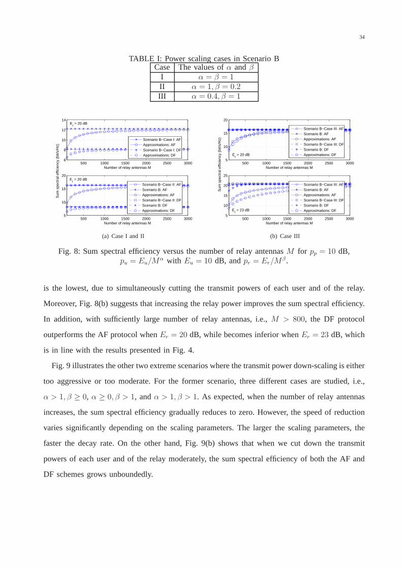
three different cases are studied according to the values ofα and β, as presented in TABLE I.
Note that the curves labelled as “Scenario B: AF” and “Scenario B: DF”, are generated by using
Theorems 5 and 8, while the curves labelled as “Scenario B-Case X: AF” and “Scenario B- Case
X: DF” with X ∈ {I, II , III } are plotted according to Corollaries 2–4 and Corollaries 8–10, for
the AF and DF protocols, respectively.
In agreement with Corollaries 2–4 and Corollaries 8–10, thesum spectral efficiency of both
the AF and DF schemes saturates in the asymptotical largeM regime for all the three cases. As
readily observed, among the three cases, the sum spectral efficiency of Case I, i.e.,α = β = 1,
34
TABLE I: Power scaling cases in Scenario BCase The values ofα andβ
I α = β = 1II α = 1, β = 0.2III α = 0.4, β = 1
500 1000 1500 2000 2500 30006
8
10
12
14
Number of relay antennas M
Scenario B−Case I: AFApproximations: AFScenario B−Case I: DFApproximations: DF
500 1000 1500 2000 2500 30005
10
15
20
Number of relay antennas M
Sum
spe
ctra
l effi
cien
cy (
bit/s
/Hz)
Scenario B−Case II: AFScenario B: AFApproximations: AFScenario B−Case II: DFScenario B: DFApproximations: DF
Er = 20 dB
Er = 20 dB
(a) Case I and II
500 1000 1500 2000 2500 30005
10
15
20
Number of relay antennas M
Sum
spe
ctra
l effi
cien
cy (
bit/s
/Hz)
Scenario B−Case III: AFScenario B: AFApproximations: AFScenario B−Case III: DFScenario B: DFApproximations: DF
500 1000 1500 2000 2500 30005
10
15
20
25
Number of relay antennas M
Scenario B−Case III: AFScenario B: AFApproximations: AFScenario B−Case III: DFScenario B: DFApproximations: DFE
r = 23 dB
Er = 20 dB
(b) Case III
Fig. 8: Sum spectral efficiency versus the number of relay antennasM for pp = 10 dB,pu = Eu/M
α with Eu = 10 dB, andpr = Er/Mβ.
is the lowest, due to simultaneously cutting the transmit powers of each user and of the relay.
Moreover, Fig. 8(b) suggests that increasing the relay power improves the sum spectral efficiency.
In addition, with sufficiently large number of relay antennas, i.e.,M > 800, the DF protocol
outperforms the AF protocol whenEr = 20 dB, while becomes inferior whenEr = 23 dB, which
is in line with the results presented in Fig. 4.
Fig. 9 illustrates the other two extreme scenarios where thetransmit power down-scaling is either
too aggressive or too moderate. For the former scenario, three different cases are studied, i.e.,
α > 1, β ≥ 0, α ≥ 0, β > 1, andα > 1, β > 1. As expected, when the number of relay antennas
increases, the sum spectral efficiency gradually reduces tozero. However, the speed of reduction
varies significantly depending on the scaling parameters. The larger the scaling parameters, the
faster the decay rate. On the other hand, Fig. 9(b) shows thatwhen we cut down the transmit
powers of each user and of the relay moderately, the sum spectral efficiency of both the AF and
DF schemes grows unboundedly.

35
500 1000 1500 2000 2500 30000
2
4
6
8
10
12
Number of relay antennas M
Sum
spe
ctra
l effi
cien
cy (
bit/s
/Hz)
Scenario B: AFApproximations: AFScenario B: DFApproximations: DFα = 0.6, β = 1.2
α = 1.3, β = 0.8
α = 1.5, β = 1.2
(a) Zero limit spectral efficiency
500 1000 1500 2000 2500 30006
8
10
12
14
16
18
20
22
24
26
Number of relay antennas M
Sum
spe
ctra
l effi
cien
cy (
bit/s
/Hz)
Scenario B: AFApproximations: AFScenario B: DFApproximations: DF
α = 0.6, β = 0.8
α = 0.9, β = 0.7
(b) Unbounded spectral efficiency
Fig. 9: Sum spectral efficiency versus the number of relay antennasM for pp = 10 dB,pu = Eu/M
α with Eu = 10 dB, andpr = Er/Mβ with Er = 20 dB.
3) Scenario C: Fig. 10 demonstrates the fundamental tradeoff between the user/relay power and
the pilot symbol power. For illustration purposes, two extreme scenarios where the transmit power
down-scaling is either too aggressive or too moderate are considered. For the former scenario, two
sets of curves are drawn according toα = 1.3, β = 1.1, γ = 0.5 andα = 0.8, β = 0.6, γ = 1,
which satisfyα + γ = 1.8 and β + γ = 1.6. When the number of relay antennas grows large,
the sum spectral efficiency of all system configurations smoothly converges to zero, as predicted.
Moreover, the gaps between the two sets of curves reduce withM and eventually vanish. This
indicates that as long asα + γ and β + γ are the same, the asymptotic sum spectral efficiency
remains unchanged. Now, let us focus on the two curves associated with the AF protocol with
N = 5. Interestingly, we see that the curve associated withγ = 0.5 yields better sum spectral
efficiency in the finite antenna regime, despite the fact thatthe user or relay power is over-reduced
compared to theγ = 1 case, which suggests that it is of crucial importance to improve the channel
estimation accuracy. The same behavior appears for the DF protocol as shown in Fig. 10(a), and
the unbounded spectral efficiency scenario as shown in Fig. 10(b).
V. POWER ALLOCATION
Power control is an effective means to enhance the sum spectral efficiency of the system. In
this section, we formulate a power allocation problem maximizing the sum spectral efficiency of

36
500 1000 1500 2000 2500 30000
0.5
1
1.5
2
2.5
3
Number of relay antennas M
Sum
spe
ctra
l effi
cien
cy (
bit/s
/Hz)
AF: α = 1.3, β = 1.1, γ = 0.5AF: α = 0.8, β = 0.6, γ = 1DF: α = 1.3, β = 1.1, γ = 0.5DF: α = 0.8, β = 0.6, γ = 1
N = 2
N = 5
(a) Zero limit spectral efficiency
0 500 1000 1500 2000 2500 30000
10
20
30
40
Number of relay antennas M
α = 0.7, β = 0.6, γ = 0.2
α = 0.4, β = 0.3, γ = 0.5
0 500 1000 1500 2000 2500 30000
10
20
30
40
Number of relay antennas M
Sum
spe
ctra
l effi
cien
cy (
bit/s
/Hz)
α = 0.5, β = 0.6, γ = 0.1
α = 0.4, β = 0.4, γ = 0.2
DF
AF N = 10
N = 10
N = 5
N = 5
(b) Unbounded spectral efficiency
Fig. 10: Sum spectral efficiency versus the number of relay antennasM for pu = Eu/Mα with
Eu = 10 dB, pr = Er/Mβ with Er = 15 dB, andpp = Ep/M
γ with Ep = 0 dB.
both the AF and DF protocols subject to a total power constraint, i.e.,N∑
i=1
(pA,i + pB,i) + pr ≤P . For notational simplicity, we defineN , {1, . . . , N}, pA , [pA,1, . . . , pA,N ]
T , and pB ,
[pB,1, . . . , pB,N ]T .
A. AF protocol
For mathematical tractability, instead of using the exact sum spectral efficiency expression in
Theorem 1, we work with the large-scale approximation from Theorem 2 which has shown be
tight for even moderateM . Thus, the power allocation optimization problem is formulated as
maximizepA,pB ,pr
τc − τpτc
N∑
i=1
(
RAFA,i + RAF
B,i
)
(126)
subject toN∑
i=1
(pA,i + pB,i) + pr ≤ P, (127)
pA ≥ 0,pB ≥ 0, pr ≥ 0, (128)
where RAFB,i is the large-scale approximation for the spectral efficiency of TB,i, which can be
derived in a similar fashion.

37
Sincelog(·) is an increasing function, (126) can be equivalently reformulated asPAF1 :
minimizepA,pB,pr
γAFA
,γAFB
N∏
i=1
(1 + γAF
A,i
)−1 (1 + γAF
B,i
)−1(129)
subject to γAFA,i ≤
pB,i
N∑
j=1
(aAFi,j pA,j + bAF
i,j pB,j
)+ p−1
r
N∑
j=1
(cAFi,j pA,j + dAF
i,j pB,j
)+ ei
, i ∈ N (130)
γAFB,i ≤
pA,i
N∑
j=1
(
aAFi,j pA,j + bAF
i,j pB,j
)
+ p−1r
N∑
j=1
(
cAFi,j pA,j + dAF
i,j pB,j
)
+ ei
, i ∈ N (131)
N∑
i=1
(pA,i + pB,i) + pr ≤ P, (132)
pA ≥ 0,pB ≥ 0, pr ≥ 0, (133)
whereγAFA ,
[γAFA,1, . . . , γ
AFA,N
]T, γAF
B ,[γAFB,1, . . . , γ
AFB,N
]TaAFi,j = 1
M
4βAR,i
σ2RB,i
, j = i,
βAR,j
σ2RB,i
+σ4AR,jσ
2RB,jβAR,i
σ4AR,iσ
4RB,i
, j 6= i,
,
bAFi,j = 1
M
βRB,i
σ2RB,i
+βAR,i
σ2AR,i
, j = i,
βRB,j
σ2RB,i
+σ2AR,jσ
4RB,jβAR,i
σ4AR,iσ
4RB,i
, j 6= i,
, cAFi,j =
σ4AR,jσ
2RB,j
Mσ4AR,iσ
4RB,i
, dAFi,j =
σ2AR,jσ
4RB,j
Mσ4AR,iσ
4RB,i
, eAFi = 1
Mσ2RB,i
,
and aAFi,j , bAF
i,j , cAFi,j , dAF
i,j , eAFi,j are obtained by replacing the subscripts “AR”, “RB” with “RB”, “AR”
in bAFi,j , aAF
i,j , dAFi,j , cAF
i,j , eAFi,j , respectively.
The above problemPAF1 is identified as a complementary geometric programming problem,
which is nonconvex [28]. Also,γAFAR,i andγAF
RB,i are considered as the signal-to-interference-plus-
noise ratio (SINR) ofRAFA,i andRAF
B,i, respectively. In addition, we have replaced the equality “=”
with “≤” in the first two constraints of problemPAF1 ; however, this does not change or relax the
original problem (126), since the objective function is decreasing with respect toγAFAR,i andγAF
RB,i.
Therefore, we can guarantee that these two constraints mustbe active at any optimal solution of
PAF1 .
It can be observed that all the inequality constraints can betransformed into posynomial
functions, hence, if the objective function is also a posynomial function, the problemPAF1 becomes
a standard GP problem, and can be solved very efficiently withstandard optimization tools such
as CVX [29] or ggplab [30]. However, the objective function is not a posynomial function.
Fortunately, capitalizing on the technique proposed in [31, Lemma 1], we can find a close local

38
optimum of the original problemPAF1 by solving a sequence of GPs. The key idea is to use a
monomial functionωAFX,i
(γAFX,i
)µAFX,i to approximate1+ γAF
X,i near an arbitrary pointγAFX,i > 0, where
X ∈ {A,B}, µAFX,i =
γAFX,i
1+γAFX,i
andωAFX,i =
(γAFX,i
)−µAFX,i(1 + γAF
X,i
). At each iteration, the GP is obtained
by replacing the posynomial objective function with its best local monomial approximation near
the solution obtained at the previous iteration. Now, we outline the successive approximation
algorithm to solve the original problemPAF1 in the following.
Algorithm 1 Successive approximation algorithm forPAF1
1) Initialization. Define a toleranceǫ and parameterθ. Setk = 1, the initial values ofγAFA,i and
γAFB,i are chosen according to the SINR in Theorem 2 when lettingpA,i = pB,i =
P4N
, andpr = P2.
2) Iteration k. ComputeµAFA,i =
γAFA,i
1+γAFA,i
andµAFB,i =
γAFB,i
1+γAFB,i
. Then, solve the following GP problem
PAF2 :
minimizepA,pB,pr
γAFA
,γAFB
N∏
i=1
(γAFA,i
)−µAFA,i(γAFB,i
)−µAFB,i
subject to θ−1γAFA,i ≤ γAF
A,i ≤ θγAFA,i, i ∈ N
θ−1γAFB,i ≤ γAF
B,i ≤ θγAFB,i, i ∈ N
γAFA,ip
−1B,i
(N∑
j=1
(aAFi,j pA,j + bAF
i,j pB,j
)+ p−1
r
N∑
j=1
(cAFi,j pA,j + dAF
i,j pB,j
)+ ei
)
≤ 1, i ∈ N
γAFB,ip
−1A,i
(N∑
j=1
(
aAFi,j pA,j + bAF
i,j pB,j
)
+ p−1r
N∑
j=1
(
cAFi,j pA,j + dAF
i,j pB,j
)
+ ei
)
≤ 1, i ∈ N
N∑
i=1
(pA,i + pB,i) + pr ≤ P,
pA ≥ 0,pB ≥ 0, pr ≥ 0. (134)
Denote the optimal solutions byγ(k),AFA,i andγ(k),AF
B,i , i ∈ N .
3) Stopping criterion. If maxi |γ(k),AFA,i − γAF
A,i| < ǫ and/ormaxi |γ(k),AFB,i − γAF
B,i| < ǫ, stop; otherwise,go to step 4).4) Update initial values. Set γAF
A,i = γ(k),AFA,i and γAF
B,i = γ(k),AFB,i , andk = k + 1. Go to step 2).
Please note, we have neglectedωAFA,i andωAF
B,i in the objective function ofPAF2 , since they are
constants and do not affect the problem solution. Also, sometrust region constraints, i.e., the first
two constraints, are added, which limit how much the variables are allowed to differ from the
current guessγAFA,i and γAF
B,i. The convergence of the above algorithm to a Karush-Kuhn-Tucker
solution of the original nonconvex problemPAF1 is guaranteed, and the detailed proof can be found

39
in [32]. The parameterθ > 1 controls the desired accuracy. More precisely, whenθ is close to 1 it
provides good accuracy for the monomial approximation but with slower convergence speed, and
vice versa ifθ is large. As discussed in [31], [33], [34],θ = 1.1 offers a good tradeoff between
the accuracy and convergence speed.
To gain further insights, we now consider the special case when all the users transmit with the
same power, i.e.,pA,i = pB,i = pu, then, the optimization problem (126) reduces to
PAF3 : maximize
pu,pr
τc − τpτc
N∑
i=1
(
RAFA,i + RAF
B,i
)
(135)
subject to 2Npu + pr ≤ P, (136)
pu ≥ 0, pr ≥ 0. (137)
Theorem 10: PAF3 is a convex optimization problem.
Proof: See Appendix IV. �
Since the optimization problemPAF3 is convex, the optimal solutionspAF,opt
u ∈(0, P
2N
]and
pAF,optr ∈ (0, P ] maximizing the sum spectral efficiency can be solved efficiently by adopting some
standard techniques, such as the bisection method with respect toP . However, it is difficult to
directly obtain closed-form expressions ofpAF,optu and pAF,opt
r , since the objective function relies
on the statistical characteristics of all the channel vectors. In order to simplify the analysis and
provide some further insights, we assume that all the users have the same large-scale fading, e.g.,
βAR,i = βRB,i = 1, thereby resulting inσ2A,i = σ2
B,i = σ2, σ2A,i = σ2
B,i = σ2, RAFA,i = RAF
B,i, and then
the optimization problemPAF3 reduces to
PAF4 : maximize
pu,pr
2N (τc − τp)
τcRAF
A,i (138)
subject to 2Npu + pr ≤ P, (139)
pu ≥ 0, pr ≥ 0. (140)
The optimal solution of the optimization problemPAF4 can be analytically characterized in the
following theorem.

40
Theorem 11: With the AF protocol, the optimization problemPAF4 is solved by
pAF,optu = P
4N,
pAF,optr = P
2.
(141)
Proof: See Appendix V. �
Theorem 11 suggests that for a given power budget2Npu + pr ≤ P , half of the total power
should be allocated to the relay regardless of the number of users, and the remaining half should
be equally allocated to the2N users. Such a symmetric power allocation strategy is ratherintuitive
due to the symmetric system setup. In addition, it can be directly inferred that the optimal power
pAF,optu decreases monotonically by increasing the number of user pairs N , which serves as a useful
guideline for practical system design.
B. DF protocol
For the DF protocol, focusing on the large-scale approximation in Theorem 3, the power
allocation optimization problem is formulated as
maximizepA,pB ,pr
τc − τpτc
N∑
i=1
RDFi (142)
subject toN∑
i=1
(pA,i + pB,i) + pr ≤ P, (143)
pA ≥ 0,pB ≥ 0, pr ≥ 0. (144)
Then, following similar procedures as the AF protocol, (142) can be equivalently reformulated

41
asPDF1 :
minimizepA,pB,pr
γDF,γDFA
,γDFB
N∏
i=1
(1 + γDF
i
)−1(145)
subject to γDFi ≤ aDF
i pA,i + bDFi pB,i
N∑
j=1
(cDFi,j pA,i + dDF
i,j pB,i
)+ 1
, i ∈ N (146)
γDFi ≤ γDF
A,i + γDFB,i + γDF
A,iγDFB,i, i ∈ N (147)
γDFA,i ≤
aDFi pA,i
N∑
j=1
(cDFi,j pA,i + dDF
i,j pB,i
)+ 1
, i ∈ N (148)
γDFA,i ≤
preDFi pr + fDF
i
, i ∈ N (149)
γDFB,i ≤
bDFi pB,i
N∑
j=1
(cDFi,j pA,i + dDF
i,j pB,i
)+ 1
, i ∈ N (150)
γDFB,i ≤
pr
eDFi pr + fDF
i
, i ∈ N (151)
N∑
i=1
(pA,i + pB,i) + pr ≤ P, (152)
pA ≥ 0,pB ≥ 0, pr ≥ 0. (153)
where γDF ,[γDF1 , . . . , γDF
N
]T, γDF
A ,[γDFA,1, . . . , γ
DFA,N
]T, γDF
B ,[γDFB,1, . . . , γ
DFB,N
]T, aDF
i =
Mσ4AR,i+σ2
AR,iσ2RB,i
σ2AR,i+σ2
RB,i
, bDFi =
Mσ4RB,i+σ2
AR,iσ2RB,i
σ2AR,i+σ2
RB,i
, cAFi,j =
σ2AR,i, j = i,
βAR,j, j 6= i,
,
eDFi =
βAR,i
Mσ4AR,i
N∑
j=1
(σ2AR,j + σ2
RB,j
), fDF
i = 1Mσ4
AR,i
N∑
j=1
(σ2AR,j + σ2
RB,j
), and dDF
i,j , eDFi , fDF
i are ob-
tained by replacing the subscripts “AR”, “RB” with “RB”, “AR” in cDFi,j , eDF
i , fDFi , respectively.
Since the objective function1+γDFi can be approximated by a monomial functionωDF
X,i
(γDFi
)µDFi ,
whereµDFi =
γDFi
1+γDFi
and ωDFi =
(γDFi
)−µDFi(1 + γDF
i
), the main challenge to convertPDF
1 into a
GP problem is to transform the first two inequality constraints into the form of posynomials.
According to [33], [35], the geometric mean is no larger thanthe arithmetic mean for any set of

42
positive numbers; thus we have
aDFi pA,i + bDF
i pB,i ≥(
aDFi pA,i
νDFA,i
)νDFA,i(
bDFi pB,i
νDFB,i
)νDFB,i
, (154)
whereνDFA,i =
aDFi pA,i
aDFi pA,i+bDF
i pB,i, νDF
B,i =bDFi pB,i
aDFi pA,i+bDF
i pB,i, and pA,i, pB,i are the initialization values.
As a result, the first inequality constraint inPDF1 can be approximated by [35]
γDFi ≤
(aDFi pA,i
νDFA,i
)νDFA,i(
bDFi pB,i
νDFB,i
)νDFB,i
N∑
j=1
(cDFi,j pA,i + dDF
i,j pB,i
)+ 1
, i ∈ N . (155)
Now, we focus on the approximation of the second inequality constraint. Following the idea
proposed in [31, Lemma 1], we use a monomial functiong(x, y) = ηxλ1yλ2 to approximate
f(x, y) = x + y + xy near an arbitrary pointx, y > 0. To make the approximation accurate, we
need to ensure that
x+ y + xy = ηxλ1 yλ2,
1 + y = ηλ1xλ1−1yλ2,
1 + x = ηλ2xλ1 yλ2−1.
(156)
As such, the parametersη, λ1, andλ2 can be computed as
λ1 =x(1+y)x+y+xy
,
λ2 =y(1+x)x+y+xy
,
η = (x+ y + xy) x−λ1 y−λ2.
(157)
To this end, the second inequality constraint inPDF1 can be approximated by
γDFi ≤ ηDF
i
(γDFA,i
)λDFA,i(γDFB,i
)λDFB,i , i ∈ N , (158)
whereηDFi =
(γDFA,i + γDF
B,i + γDFA,iγ
DFB,i
) (γDFA,i
)−λDFA,i(γDFB,i
)−λDFB,i , λDF
A,i =γDFA,i(1+γDF
B,i)γDFA,i+γDF
B,i+γDFA,iγ
DFB,i
,
λDFB,i =
γDFB,i(1+γDF
A,i)γDFA,i+γDF
B,i+γDFA,iγ
DFB,i
, and γDFA,i, γ
DFB,i are the initialization values.
We now outline the successive approximation algorithm to solve the original problemPDF1 as
follows.

43
Algorithm 2 Successive approximation algorithm forPDF1
1) Initialization. Define a toleranceǫ and parameterθ. Setk = 1, the initial values ofγDFi , γDF
A,i
and γDFB,i are chosen according to the SINR in Theorem 3. Also, we setpA,i = pB,i =
P4N
,
2) Iteration k. ComputeµDFi =
γDFi
1+γDFi
, νDFA,i =
aDFi pA,i
aDFi pA,i+bDF
i pB,i, νDF
B,i =bDFi pB,i
aDFi pA,i+bDF
i pB,i, ηDF
i =(γDFA,i + γDF
B,i + γDFA,iγ
DFB,i
) (γDFA,i
)−λDFA,i(γDFB,i
)−λDFB,i , λDF
A,i =γDFA,i(1+γDF
B,i)γDFA,i+γDF
B,i+γDFA,iγ
DFB,i
, λDFB,i =
γDFB,i(1+γDF
A,i)γDFA,i+γDF
B,i+γDFA,iγ
DFB,i
.
Then, solve the following GP problemPDF2 :
minimizepA,pB,pr
γDF,γDFA
,γDFB
N∏
i=1
(γDFi
)−µDFi
subject to θ−1pDFA,i ≤ pDF
A,i ≤ θpDFA,i, i ∈ N
θ−1pDFB,i ≤ pDF
B,i ≤ θpDFB,i, i ∈ N
θ−1γDFi ≤ γDF
i ≤ θγDFi , i ∈ N
θ−1γDFA,i ≤ γDF
A,i ≤ θγDFA,i, i ∈ N
θ−1γDFB,i ≤ γDF
B,i ≤ θγDFB,i, i ∈ N
γDFi
(
aDFi pA,i
νDFA,i
)−νDFA,i(
bDFi pB,i
νDFB,i
)−νDFB,i(
N∑
j=1
(cDFi,j pA,i + dDF
i,j pB,i
)+ 1
)
≤ 1, i ∈ N ,
γDFi
(ηDFi
)−1 (γDFA,i
)−λDFA,i(γDFB,i
)−λDFB,i ≤ 1, i ∈ N ,
γDFA,i
(aDFi
)−1p−1A,i
(N∑
j=1
(cDFi,j pA,i + dDF
i,j pB,i
)+ 1
)
≤ 1, i ∈ N
γDFA,ip
−1r
(eDFi pr + fDF
i
)≤ 1, i ∈ N
γDFB,i
(bDFi
)−1p−1B,i
(N∑
j=1
(cDFi,j pA,i + dDF
i,j pB,i
)+ 1
)
≤ 1, i ∈ N
γDFB,ip
−1r
(
eDFi pr + fDF
i
)
≤ 1, i ∈ NN∑
i=1
(pA,i + pB,i) + pr ≤ P,
pA ≥ 0,pB ≥ 0, pr ≥ 0. (159)
Denote the optimal solutions byp(k),DFA,i , p(k),DF
B,i , γ(k),DFi , γ(k),DF
A,i , γ(k),DFB,i , i ∈ N .
3) Stopping criterion. If maxi |p(k),DFA,i − pDF
A,i| < ǫ and/or maxi |p(k),DFB,i − pDF
B,i| < ǫ and/or
maxi |γ(k),DFi − γDF
i | < ǫ and/ormaxi |γ(k),DFA,i − γDF
A,i| < ǫ and/ormaxi |γ(k),DFB,i − γDF
B,i| < ǫ, stop;otherwise, go to step 4).4) Update initial values. Set pDF
A,i = p(k),DFA,i , pDF
B,i = p(k),DFB,i , γDF
i = γ(k),DFi , γDF
A,i = γ(k),DFA,i , γDF
B,i =
γ(k),DFB,i , andk = k + 1. Go to step 2).
Similar to algorithms for the AF protocol, we have removedωDFi in the objective function, since
they do not affect the optimization problem. Also, five extrainequalities as trust region constraints

44
are included.
Algorithm 2 focuses on the case where each user transmits with a different power, and yields a
close local optimum of the original problemPDF1 by solving a sequence of GPs. Now, we turn our
attention to the scenario where all the users transmit with the same power, i.e.,pA,i = pB,i = pu;
hence, the problem (142) reduces to the following special case:
PDF3 : maximize
pu,pr
τc − τpτc
N∑
i=1
RDFi (160)
subject to 2Npu + pr ≤ P, (161)
pu ≥ 0, pr ≥ 0. (162)
Theorem 12: PDF3 is a convex optimization problem.
Proof: See Appendix VI. �
Similar to the AF protocol, the optimal solutionspDF,optu ∈
(0, P
2N
]andpDF,opt
r ∈ (0, P ] maximiz-
ing the sum spectral efficiency can be solved efficiently by adopting some standard techniques,
such as the bisection method with respect toP , due to the convexity of the optimization problem
PDF3 .
C. Numerical Results
Fig. 11 illustrates the impact of the optimal power allocation scheme on the sum spectral
efficiency when all users’ large-scale fading are different. The different large-scale fading param-
eters are arbitrarily generated byβAR,i = zi (rAR,i/r0)α and βRB,i = zi (rBR,i/r0)
α, wherezi is
a log-normal random variable with standard deviation8 dB, rAR,i and rRB,i are the locations
of TAR,i and TRB,i from the relay,α = 3.8 is the path loss exponent, andr0 denotes the
guard interval which specifies the nearest distance betweenthe users and the relay. The relay
is located at the center of a cell with a radius of1000 meters andr0 = 100 meters. We
chooseP = 10 dB, pp = 10 dB, N = 5, βAR = [0.2688, 0.0368, 0.00025, 0.1398, 0.0047],
and βRB = [0.0003, 0.00025, 0.0050, 0.0794, 0.0001]. The optimal power allocation curves are
generated by Algorithm 1 and Algorithm 2. As a benchmark scheme for comparison, we also plot
the sum spectral efficiency with uniform power allocation, i.e., the relay transmit power equals to
the sum user transmit power. Please note that such a uniform power allocation scheme is optimal

45
for the AF protocol when all the users have the same large-scale fading parameters, as shown in
Theorem 11. As can be observed, the optimal power allocationpolicy provides 34.8% and 89.2%
spectral efficiency enhancement whenM = 300, for the AF and DF protocols, respectively. This
suggests that the improvement of the DF protocol is more prominent.
100 200 300 400 500 600 700 800 900 10000
1
2
3
4
5
6
Number of relay antennas M
Sum
spe
ctra
l effi
cien
cy (
bit/s
/Hz)
Optimal power allocation: AFUniform power allocation: AFOptimal power allocation: DFUniform power allocation: DF
Fig. 11: Sum spectral efficiency versus the number of relay antennasM for P = 10 dB, pp = 10dB andN = 5.
Fig. 12 examines the impact of key system parameters such asM , N , andpp on the optimal
power allocation scheme when every user has the same transmit power, i.e,pA,i = pB,i = pu. As
expected, for a given power budgetP = 10 dB, the optimal user transmit power is a decreasing
function with respect to the number of user pairsN for both the AF and DF protocols, as shown
in Fig. 12(a). Then, we focus on the DF protocol and depict theoutcomes in Fig. 12(b). As can be
seen, with fixed number of user pairsN = 5, the optimal user transmit power for the DF protocol
pDF,optu with M = 100 is larger than that withM = 50, suggesting that we should increase the
transmit power of each user when the number of relay antennasis large. In addition, when the
pilot training power increases, i.e., frompp = −20 dB to pp = 0 dB, the optimal user transmit
power pDF,optu also increases, indicating that when the channel estimation accuracy is improved,
we need to use a higher transmit power for each user.
VI. CONCLUSION
We have investigated the sum spectral efficiency of a multipair two-way half-duplex relaying
system employing the MR scheme taking into account of realistic CSI assumption. In particular,

46
−10 −8 −6 −4 −2 00
1
2
3
4
5
6
7
8
9
pu (dB)
Sum
spe
ctra
l effi
cien
cy (
bit/s
/Hz)
AFDF
N = 10
N = 5
−6
−3
−3.3
−0.3
(a) AF and DF
−10 −8 −6 −4 −2 00
2
4
6
8
10
M = 100M = 50
−10 −8 −6 −4 −2 00
2
4
6
8
pu (dB)
Sum
spe
ctra
l effi
cien
cy (
bit/s
/Hz)
pp = 0 dB
pp = −20 dB
−0.3
−0.3
−0.4
−0.2
(b) DF
Fig. 12: Sum spectral efficiency versuspu for P = 10 dB (pp = 0 dB, M = 50 andN = 5unless otherwise specified).
an exact expression was derived for the sum spectral efficiency of the AF protocol and closed-form
large-scale approximations of the spectral efficiency for both AF and DF protocols were obtained
when the number of relay antennas is large. Based on these expressions, a detailed comparison
between the AF and DF protocols was conducted, and it was shown that the spectral efficiency
of the AF protocol is more sensitive in scenarios with low transmit power of the relay and pilot
symbol, small number of relay antennas, and large number of user pairs. Moreover, power scaling
laws of the system were characterized, which showed that thetransmit powers of user, relay,
and pilot symbol can be scaled down inversely proportional to the number of relay antennas. In
addition, it was revealed that there exists a fundamental tradeoff between the user/relay transmit
power and pilot symbol power, which provides great flexibility for the design of practical systems.
Finally, the transmit powers of each user and the relay were optimized to enhance the sum spectral
efficiency.
APPENDIX I
PROOF OFTHEOREM 1
The end-to-end SINR given in (25) consists of five terms: 1) desired signal powerAAFi ;
2) estimation errorBAFi ; 3) residual self-interferenceCAF
i ; 4) inter-user interferenceDAFi ; 5)
compound noiseEAFi .

47
We start by first rewritingF as
F =N∑
n=1
(g∗RB,ng
HAR,n + g∗
AR,ngHRB,n
). (163)
After substituting (163) into (25), we compute the five termsone by one.
1) ComputeAAFi :
E
{gTAR,iFgRB,i
}= E
{N∑
n=1
(gTAR,ig
∗RB,ng
HAR,ngRB,i + gT
AR,ig∗AR,ng
HRB,ngRB,i
)
}
, (164)
= E
{(gTAR,ig
∗RB,ig
HAR,igRB,i + gT
AR,ig∗AR,ig
HRB,igRB,i
)},
= E
{|gH
AR,igRB,i|2 + ||gAR,i||2||gRB,i||2},
= Mσ2AR,iσ
2RB,i +M2σ2
AR,iσ2RB,i.
Consequently, we obtain
AAFi = pB,iM
2(M + 1)2σ4AR,iσ
4RB,i. (165)
2) ComputeBAFi :
E
{|gT
AR,iFgRB,i|2}
(166)
= E
{N∑
n=1
N∑
l=1
gTAR,i
(g∗RB,ng
HAR,n + g∗
AR,ngHRB,n
)gRB,ig
HRB,i
(gAR,lg
TRB,l + gRB,lg
TAR,l
)g∗AR,i
}
,
which can be decomposed into three different cases:
a) for n 6= l 6= i, we haveE{|gT
AR,iFgRB,i|2}= 0.
b) for n = l 6= i, we have
E
{|gT
AR,iFgRB,i|2}
(167)
= E
{N∑
n=1
gTAR,i
(g∗RB,ng
HAR,n + g∗
AR,ngHRB,n
)gRB,ig
HRB,i
(gAR,ng
TRB,n + gRB,ng
TAR,n
)g∗AR,i
}
.
SincegAR,i, gRB,i, gAR,i, andgRB,i are independent of each other, we can take expectation over
the four vectors separately. Utilizing the fact thatE
{gRB,ig
HRB,i
}= βRB,iIM , E
{gTAR,ig
∗AR,i
}=

48
MβAR,i, and
E
{(g∗RB,ng
HAR,n + g∗
AR,ngHRB,n
) (gAR,ng
TRB,n + gRB,ng
TAR,n
)}(168)
= E
{g∗RB,ng
HAR,ngAR,ng
TRB,n
}+ E
{g∗RB,ng
HAR,ngRB,ng
TAR,n
}+ E
{g∗AR,ng
HRB,ngAR,ng
TRB,n
}
+ E
{g∗AR,ng
HRB,ngRB,ng
TAR,n
},
= Mσ2AR,nσ
2RB,nIM + σ2
AR,nσ2RB,nIM + σ2
AR,nσ2RB,nIM +Mσ2
AR,nσ2RB,nIM ,
= 2 (M + 1)σ2AR,nσ
2RB,nIM ,
we have
E
{|gT
AR,iFgRB,i|2}= 2M (M + 1)βAR,iβRB,i
N∑
n=1
σ2AR,nσ
2RB,n. (169)
c) for n = l = i, we have
E
{|gT
AR,iFgRB,i|2}
(170)
= E
{gTAR,i
(g∗RB,ig
HAR,i + g∗
AR,igHRB,i
)gRB,ig
HRB,i
(gAR,ig
TRB,i + gRB,ig
TAR,i
)g∗AR,i
},
= E
{gTAR,ig
∗RB,ig
HAR,igRB,ig
HRB,igAR,ig
TRB,ig
∗AR,i
}+ E
{gTAR,ig
∗RB,ig
HAR,igRB,ig
HRB,igRB,ig
TAR,ig
∗AR,i
}
+ E
{gTAR,ig
∗AR,ig
HRB,igRB,ig
HRB,igAR,ig
TRB,ig
∗AR,i
}+ E
{gTAR,ig
∗AR,ig
HRB,igRB,ig
HRB,igRB,ig
TAR,ig
∗AR,i
}.
The first term in (170) becomes
E
{gTAR,ig
∗RB,ig
HAR,igRB,ig
HRB,igAR,ig
TRB,ig
∗AR,i
}(171)
= E
{gTAR,ig
∗RB,ig
HAR,igRB,ig
HRB,igAR,ig
TRB,ig
∗AR,i
}+ E
{eTAR,ig
∗RB,ig
HAR,igRB,ig
HRB,igAR,ig
TRB,ie
∗AR,i
}
+ E
{gTAR,ig
∗RB,ig
HAR,ieRB,ie
HRB,igAR,ig
TRB,ig
∗AR,i
}+ E
{eTAR,ig
∗RB,ig
HAR,ieRB,ie
HRB,igAR,ig
TRB,ie
∗AR,i
},
= E
{|gH
AR,igRB,i|4}+ σ2
AR,iE
{|gH
AR,igRB,i|2||gRB,i||2}+ σ2
RB,iE
{|gH
AR,igRB,i|2||gAR,i||2}
+ σ2RB,iE
{|gH
RB,ieAR,i|2||gAR,i||2},
= E
{|gAR,i|4||gRB,i||4
}+ σ2
AR,iE
{|gAR,i|2||gRB,i||4
}+ σ2
RB,iE
{|gRB,i|2||gAR,i||4
}
+ σ2RB,iE
{|gH
RB,ieAR,i|2}E
{||gAR,i||2
},
where gAR,i ,gHAR,igRB,i
||gRB,i||and gRB,i ,
gHAR,igRB,i
||gAR,i||. Conditioned ongRB,i, gAR,i is a Gaussian

49
random variable with zero mean and varianceσ2AR,i which does not depend ongRB,i whereas
conditioned ongAR,i, gRB,i is a Gaussian random variable with zero mean and varianceσ2RB,i which
does not depend ongAR,i. Therefore, we haveE {|gAR,i|4||gRB,i||4} = E {|gAR,i|4} E {||gRB,i||4},
E {|gAR,i|2||gRB,i||4} = E {|gAR,i|2} E {||gRB,i||4}, andE {|gRB,i|2||gAR,i||4} = E {|gRB,i|2} E {||gAR,i||4}.
Then, by using the fact thatE {|gAR,i|4} = 2σ4AR,i, E {|gRB,i|2} = σ4
RB,i, and E {||gRB,i||4} =
M(M + 1)σ4RB,i, (171) can be calculated as
E
{gTAR,ig
∗RB,ig
HAR,igRB,ig
HRB,igAR,ig
TRB,ig
∗AR,i
}(172)
= 2σ4AR,iM (M + 1)σ4
RB,i + σ2AR,iσ
2AR,iM (M + 1) σ4
RB,i
+ σ2RB,iσ
2RB,iM (M + 1)σ4
AR,i + σ2RB,iσ
2AR,iσ
2RB,iM
2σ2AR,i,
= M (M + 1)σ2AR,iσ
2RB,i
(βAR,iσ
2RB,i + βRB,iσ
2AR,i
)+M2σ2
AR,iσ2RB,iσ
2AR,iσ
2RB,i.
Following the same procedure, the last three terms in (170) can be calculated as
E
{gTAR,ig
∗RB,ig
HAR,igRB,ig
HRB,igRB,ig
TAR,ig
∗AR,i
}(173)
= M (M + 1)2 σ4AR,iσ
4RB,i +M (M + 1) σ4
AR,iσ2AR,iσ
2RB,i
+M (M + 1)σ2AR,iσ
2AR,iσ
4RB,i +Mσ2
AR,iσ2AR,iσ
2RB,iσ
2RB,i,
E
{gTAR,ig
∗AR,ig
HRB,igRB,ig
HRB,igAR,ig
TRB,ig
∗AR,i
}(174)
= M (M + 1)2 σ4AR,iσ
4RB,i +M (M + 1) σ4
AR,iσ2AR,iσ
2RB,i
+M (M + 1)σ2AR,iσ
2AR,iσ
4RB,i +Mσ2
AR,iσ2AR,iσ
2RB,iσ
2RB,i,
E
{gTAR,ig
∗AR,ig
HRB,igRB,ig
HRB,igRB,ig
TAR,ig
∗AR,i
}(175)
= M2 (M + 1)2 σ4AR,iσ
4RB,i +M2 (M + 1)σ4
AR,iσ2AR,iσ
2RB,i
+M2 (M + 1)σ2AR,iσ
2AR,iσ
4RB,i +M2σ2
AR,iσ2AR,iσ
2RB,iσ
2RB,i.

50
Finally, combining a), b), and c), we obtain
BAFi = pB,iE
{|gT
AR,iFgRB,i|2}− pB,iM
2 (M + 1)2 σ4AR,iσ
4RB,i, (176)
= pB,i2M (M + 1)βAR,iβRB,i
N∑
n=1
σ2AR,nσ
2RB,n
+ pB,iM (M + 1)σ2AR,iσ
2RB,i
(βAR,iσ
2RB,i + βRB,iσ
2AR,i
)+ pB,iM
2σ2AR,iσ
2RB,iσ
2AR,iσ
2RB,i
+ pB,i2M (M + 1)2 σ4AR,iσ
4RB,i + pB,i2M (M + 1)σ4
AR,iσ2AR,iσ
2RB,i + pB,i2M (M + 1)σ2
AR,iσ2AR,iσ
4RB,i
+ pB,i2Mσ2AR,iσ
2AR,iσ
2RB,iσ
2RB,i + pB,iM
2 (M + 1)σ4AR,iσ
2AR,iσ
2RB,i
+ pB,iM2 (M + 1) σ2
AR,iσ2AR,iσ
4RB,i + pB,iM
2σ2AR,iσ
2AR,iσ
2RB,iσ
2RB,i.
3) ComputeCAFi :
By utilizing the same technique as in the derivation ofBAFi , we have
a) for n 6= l 6= i, we haveE{|gT
AR,iFgAR,i|2}= 0.
b) for n = l 6= i, we have
E
{|gT
AR,iFgAR,i|2}
(177)
= E
{N∑
n=1
gTAR,i
(g∗RB,ng
HAR,n + g∗
AR,ngHRB,n
)gAR,ig
HAR,i
(gAR,ng
TRB,n + gRB,ng
TAR,n
)g∗AR,i
}
,
= 4M(M + 1)β2AR,i
N∑
n=1
σ2AR,nσ
2RB,n.
c) for n = l = i, we have
E
{|gT
AR,iFgAR,i|2}
(178)
= E
{gTAR,i
(g∗RB,ig
HAR,i + g∗
AR,igHRB,i
)gAR,ig
HAR,i
(gAR,ig
TRB,i + gRB,ig
TAR,i
)g∗AR,i
},
= 4σ2AR,iσ
2RB,iM (M + 1)
((M + 2) σ4
AR,i + (M + 5) σ2AR,iσ
2AR,i + σ4
AR,i
).
Then, by using the following fact
E
{gTAR,iFgAR,i
}= 0, (179)

51
we have
CAFi = 4pA,iM(M + 1)β2
AR,i
N∑
n=1
σ2AR,nσ
2RB,n (180)
+ 4pA,iσ2AR,iσ
2RB,iM (M + 1)
((M + 2)σ4
AR,i + (M + 5)σ2AR,iσ
2AR,i + σ4
AR,i
).
4) ComputeDAFi :
E
{|gT
AR,iFgAR,j |2}
(181)
= E
{N∑
n=1
N∑
l=1
gTAR,i
(g∗RB,ng
HAR,n + g∗
AR,ngHRB,n
)gAR,jg
HAR,j
(gAR,lg
TRB,l + gRB,lg
TAR,l
)g∗AR,i
}
,
which can be decomposed into six different cases:
a) for n 6= l 6= i, j (j 6= i), we haveE{|gT
AR,iFgAR,j |2}= 0.
b) for n = l 6= i, j (j 6= i), we have
E
{|gT
AR,iFgAR,j |2}
(182)
= E
{∑
n 6=i,j
gTAR,i
(g∗RB,ng
HAR,n + g∗
AR,ngHRB,n
)gAR,jg
HAR,j
(gAR,ng
TRB,n + gRB,ng
TAR,n
)g∗AR,i
}
,
= 2M (M + 1)βAR,iβAR,j
∑
n 6=i,j
σ2AR,nσ
2RB,n.
c) for n = l = i (j 6= i), we have
E
{|gT
AR,iFgAR,j |2}
(183)
= E
{gTAR,i
(g∗RB,ig
HAR,i + g∗
AR,igHRB,i
)gAR,jg
HAR,j
(gAR,ig
TRB,i + gRB,ig
TAR,i
)g∗AR,i
},
= MβAR,jσ2AR,iσ
2RB,i
((M + 1) (M + 3)σ2
AR,i + 2 (M + 1) σ2AR,i
).
d) for n = l = j (j 6= i), we have
E
{|gT
AR,iFgAR,j |2}
(184)
= E
{gTAR,i
(g∗RB,j g
HAR,j + g∗
AR,j gHRB,j
)gAR,jg
HAR,j
(gAR,jg
TRB,j + gRB,j g
TAR,j
)g∗AR,i
},
= MβAR,iσ2AR,jσ
2RB,j
((M + 1) (M + 3)σ2
AR,j + 2 (M + 1) σ2AR,j
).
e) for n = i and l = j (j 6= i), we haveE{|gT
AR,iFgAR,j |2}= 0.

52
f) for n = j and l = i (j 6= i), we haveE{|gT
AR,iFgAR,j |2}= 0.
Altogether,E{|gT
AR,iFgAR,j |2}
is given by
E
{gTAR,iFgAR,j
}= 2M (M + 1)βAR,iβAR,j
∑
n 6=i,j
σ2AR,nσ
2RB,n (185)
+MβAR,jσ2AR,iσ
2RB,i
((M + 1) (M + 3) σ2
AR,i + 2 (M + 1) σ2AR,i
)
+MβAR,iσ2AR,jσ
2RB,j
((M + 1) (M + 3)σ2
AR,j + 2 (M + 1) σ2AR,j
).
Following the same technique as in deriving (185), we can obtain
E
{|gT
AR,iFgRB,j |2}= 2M (M + 1)βAR,iβRB,j
∑
n 6=i,j
σ2AR,nσ
2RB,n (186)
+MβRB,jσ2AR,iσ
2RB,i
((M + 1) (M + 3) σ2
AR,i + 2 (M + 1) σ2AR,i
)
+MβAR,iσ2AR,jσ
2RB,j
((M + 1) (M + 3)σ2
RB,j + 2 (M + 1) σ2RB,j
).
As a result, combining (185) and (186) yields
DAFi =
∑
j 6=i
2M (M + 1)βAR,i (pA,iβAR,j + pB,iβRB,j)∑
n 6=i,j
σ2AR,nσ
2RB,n (187)
+∑
j 6=i
Mσ2AR,iσ
2RB,i (pA,iβAR,j + pB,iβRB,j)
((M + 1) (M + 3) σ2
AR,i + 2 (M + 1) σ2AR,i
)
+∑
j 6=i
MβAR,iσ2AR,jσ
2RB,j
((M + 1) (M + 3)
(pA,iσ
2AR,j + pB,iσ
2RB,j
)+ 2 (M + 1)
(pA,iσ
2AR,j + pB,iσ
2RB,j
)).
5) ComputeEAFi :
(a) ComputeE{||gT
AR,iF||2}
:
Again, using the same technique as in the derivation of (185), we obtain
E
{||gT
AR,iF||2}= 2M (M + 1)βAR,i
∑
n 6=i
σ2AR,nσ
2RB,n (188)
+Mσ2AR,iσ
2RB,i
((M + 1) (M + 3)σ2
AR,i + 2 (M + 1) σ2AR,i
).

53
(b) ComputeE {||FgAR,i||2} andE {||FgRB,i||2}:
E
{||FgAR,i||2
}= 2M (M + 1)βAR,i
∑
n 6=i
σ2AR,nσ
2RB,n (189)
+Mσ2AR,iσ
2RB,i
((M + 1) (M + 3)σ2
AR,i + 2 (M + 1) σ2AR,i
).
Similarly, we have
E
{||FgRB,i||2
}= 2M (M + 1)βRB,i
∑
n 6=i
σ2AR,nσ
2RB,n (190)
+Mσ2AR,iσ
2RB,i
((M + 1) (M + 3) σ2
RB,i + 2 (M + 1) σ2RB,i
).
(c) ComputeE {||F||2F}:
E
{||F||2F
}= E
{tr(ABTB∗AH
}), (191)
= tr(
E
{
GARGRBG∗RBG
HAR
})
+ tr(
E
{
GARGRBG∗ARG
HRB
})
+ tr(
E
{
GRBGARG∗RBG
HAR
})
+ tr(
E
{
GRBGARG∗ARG
HRB
})
,
= 2M (M + 1)
N∑
n=1
σ2AR,nσ
2RB,n.
Combining (189), (190) and (191),ρ2AF is expressed as
ρ2AF =pr
N∑
i=1
(ai + bi) + 2M (M + 1)N∑
n=1
σ2AR,nσ
2RB,n
, (192)
whereai = Mσ2AR,iσ
2RB,i
((M + 1) (M + 3)
(σ2AR,ipA,i + σ2
RB,ipB,i
)+ 2 (M + 1)
(σ2AR,ipA,i + σ2
RB,ipB,i
)),
bi = 2M (M + 1) (βAR,ipA,i + βRB,ipB,i)∑
n 6=i
σ2AR,nσ
2RB,n.
We arrive at the desired resultEAFi by combining (188) and (192).
APPENDIX II
PROOF OFTHEOREM 3
Here we only present the detailed derivation forRDF1,i andRDF
RA,i, sinceRDFAR,i and RDF
BR,i can be
obtained in a relatively straightforward way, whileRDFRB,i can be derived in the same fashion as
RDFRA,i.

54
First, we focus on (50), which consists of five terms: 1) desired signal power of TB,i ADFi ;
2) desired signal power of TA,i BDFi ; 3) estimation errorCDF
i ; 4) inter-user interferenceDDFi ; 5)
compound noiseEDFi . For each of these five terms, we will subsequently derive a deterministic
equivalent expression.
Before proceeding, we first review some useful results, which are given in the following lemma.
Lemma 1: Let x ∼ CN (0, σ2xIM) andy ∼ CN (0, σ2
yIM). Assume thatx andy are mutually
independent. Then, we have
1
Mx†x
a.s.→ σ2x, M → ∞, (193)
1
Mx†y
a.s.→ 0, M → ∞, (194)
1
M2|x†y|2 − 1
Mσ2xσ
2y
a.s.→ 0, M → ∞. (195)
Now, we compute the five terms one by one.
1) Deterministic equivalent forADFi :
ADFi = M2pA,i
(1
M2|gH
AR,igAR,i|2 +1
M2|gH
RB,igAR,i|2)
. (196)
By invoking Lemma 1, we have
ADFi −MpA,i
(Mσ4
AR,i + σ2AR,iσ
2RB,i
) a.s.→ 0. (197)
2) Deterministic equivalent forBDFi :
BDFi = M2pB,i
(1
M2|gH
AR,igRB,i|2 +1
M2|gH
RB,igRB,i|2)
. (198)
Similarly, we obtain
BDFi −MpB,i
(Mσ4
RB,i + σ2AR,iσ
2RB,i
) a.s.→ 0. (199)
3) Deterministic equivalent forCDFi :

55
Since
CDFi = M2pA,i
(1
M2|gH
AR,ieAR,i|2 +1
M2|gH
RB,ieAR,i|2)
(200)
+M2pB,i
(1
M2|gH
AR,ieRB,i|2 +1
M2|gH
RB,ieRB,i|2)
,
we have
CDFi −M
(σ2AR,i + σ2
RB,i
) (pA,iσ
2AR,i + pB,iσ
2RB,i
) a.s.→ 0. (201)
4) Deterministic equivalent forDDFi :
For j 6= i, we have
DDFi = M2
∑
j 6=i
pA,j
(1
M2|gH
AR,igAR,j|2 +1
M2|gH
RB,igAR,j |2)
(202)
+M2∑
j 6=i
pB,j
(1
M2|gH
AR,igRB,j |2 +1
M2|gH
RB,igRB,j |2)
.
To this end, we obtain
DDFi −M
∑
j 6=i
(pA,j
(σ2AR,iβAR,j + σ2
RB,iβAR,j
)+ pB,j
(σ2AR,iβRB,j + σ2
RB,iβRB,j
)) a.s.→ 0. (203)
5) Deterministic equivalent forEDFi :
EDFi = M2
(1
M2|gAR,i|2 +
1
M2|gRB,i|2
)
. (204)
Then, employing Lemma 1 yields
EDFi −M
(σ2AR,i + σ2
RB,i
) a.s.→ 0. (205)
Substituting (197), (199), (201), (203), and (205) into (50), (56), and after some algebraic
manipulations, we obtainRDF1,i , R
DFAR,i, R
DFBR,i.
Now, we turn our attention to deriveRDFRA,i.
1) ComputeE{gTAR,ig
∗AR,i
}:
E
{gTAR,ig
∗AR,i
}= E
{||gAR,i||2
}+ E
{eTAR,ig
∗AR,i
}= Mσ2
AR,i. (206)

56
2) Compute Var(gTAR,ig
∗AR,i
)
Var(gTAR,ig
∗AR,i
)= E
{|gT
AR,ig∗AR,i|2
}−M2σ4
AR,i, (207)
= E
{||gAR,i||4
}+ E
{|eTAR,ig
∗AR,i|2
}−M2σ4
AR,i,
= M(M + 1)σ4AR,i +Mσ2
AR,iσ2AR,i −M2σ4
AR,i,
= Mσ2AR,iβAR,i.
3) Compute Var(gTAR,ig
∗RB,i
):
Var(gTAR,ig
∗RB,i
)= E
{|gT
AR,ig∗RB,i|2
}− |E
{gTAR,ig
∗RB,i
}|2, (208)
= Mσ2RB,iβAR,i.
4) Compute∑
j 6=i
(E
{|gT
AR,ig∗RB,j |2
}+ E
{|gT
AR,ig∗AR,j|2
}):
For j 6= i, we obtain
E
{|gT
AR,ig∗RB,j |2
}= Mσ2
RB,jβAR,i, (209)
and
E
{|gT
AR,ig∗AR,j |2
}= Mσ2
AR,jβAR,i. (210)
Thus, we have
∑
j 6=i
(E
{|gT
AR,ig∗RB,j |2
}+ E
{|gT
AR,ig∗AR,j|2
})= MβAR,i
∑
j 6=i
(σ2AR,j + σ2
RB,j
). (211)
Combining (206), (207), (208), and (211) completes the proof.
APPENDIX III
PROOF OFTHEOREM 4
With fixed Ep, whenpp =Ep
Mγ andγ > 0, asM → ∞, we have
σ2AR,i −
τpEpβ2AR,i
Mγ
a.s.→ 0, σ2AR,i
a.s.→ βAR,i, (212)
σ2RB,i −
τpEpβ2RB,i
Mγ
a.s.→ 0, σ2RB,i
a.s.→ βRB,i. (213)

57
Substituting (212) into (37), we have
BAFi − Mγ
τpEp
(1
βRB,i
+1
βAR,i
)
a.s.→ 0, (214)
CAFi − Mγ
τpEp
4β2AR,i
β2RB,i
a.s.→ 0, (215)
DAFi − Mγ
τpEp
∑
j 6=i
(
βAR,j + βRB,j
β2RB,i
+β4AR,jβ
2RB,jβAR,i + β2
AR,jβ4RB,jβRB,i
β4AR,iβ
4RB,i
)
a.s.→ 0, (216)
EAFi − Mγ
τpEp
(
1
puβ2RB,i
+1
prβ4AR,iβ
4RB,i
N∑
n=1
(β2AR,nβ
2RB,n
(β2AR,n + β2
RB,n
))
)
a.s.→ 0. (217)
Therefore, we have now proved thatRAFA,i−RAF
A,i
M→∞−→ 0. Since we know thatRAFA,i−RAF
A,i
M→∞−→ 0,
this implies that alsoRAFA,i − RAF
A,i
M→∞−→ 0.
APPENDIX IV
PROOF OFTHEOREM 10
For a givenpu, the objective function of the optimization problemPAF3 is an increasing function
with respect topp, while for a givenpp, this function is an increasing function with respect topu;
hence, the objective function is maximized when2Npu + pr = P [36].
Now, focusing onRAFA,i and substituting2Npu + pr = P into RAF
A,i, we have
RAFA,i =
1
2log2
(
1 +1
a+ bpu
+ cd−pu
)
, (218)
wherea = 1M
(
βRB,i+4βAR,i
σ2RB,i
+βAR,i
σ2AR,i
+∑
j 6=i
(βAR,j
σ2RB,i
+σ4AR,jσ
2RB,jβAR,i
σ4AR,iσ
4RB,i
)
+∑
j 6=i
(βRB,j
σ2RB,i
+σ2AR,jσ
4RB,jβAR,i
σ4AR,iσ
4RB,i
))
,
b = 1Mσ2
RB,i
, c = 12MNσ4
AR,iσ4RB,i
N∑
n=1
(σ2AR,nσ
2RB,n
(σ2AR,n + σ2
RB,i
)), andd = P
2N.

58
Taking the second derivative with respect topu yields
∂RAFA,i
∂pu(219)
= − b2(2cd2 + (1 + 2a) (d− pu)
3) (d− pu)
2 ln 2 (b (d− pu) + (c+ a (d− pu)) pu)2 (b (d− pu) + (c+ (1 + a) (d− pu)) pu)
2
− c (c + 2ac+ 2a (1 + a) (d− pu)) p4u
2 ln 2 (b (d− pu) + (c+ a (d− pu)) pu)2 (b (d− pu) + (c+ (1 + a) (d− pu)) pu)
2
− bpu(c2d2 + a (1 + a) (d− pu)
4 + (1 + 2a) c (d− pu) (d2 − dpu + p2u)
)
ln 2 (b (d− pu) + (c + a (d− pu)) pu)2 (b (d− pu) + (c+ (1 + a) (d− pu)) pu)
2 < 0.
Thus, RAFA,i is a strictly concave function with respect topu. Since nonnegative weighted sums
preserve convexity [37], the objective functionτc−τpτc
N∑
i=1
(
RAFA,i + RAF
B,i
)
is also a strictly concave
function with respect topu. Recall that the constraints of the optimization problemPAF3 are all
affine functions, and hencePAF3 is a convex optimization problem.
APPENDIX V
PROOF OFTHEOREM 11
Substitutingσ2A,i = σ2
B,i = σ2, σ2A,i = σ2
B,i = σ2, RAFA,i = RAF
B,i into the objective function in
PAF4 , after some simple algebraic manipulations,PAF
4 reduces to
argmaxpu
{log2 (1 +M/f(pu))} (220)
s.t. 0 ≤ pu ≤ P
2N, (221)
wheref(pu) = a + bpu
+ cP−2Npu
with a = 1σ2 (4N + 2), b = 1
σ2 , andc = 2Nσ2 .
It is easy to show thatf ′′(pu) = 2bp3u
+ 8N2c
(P−2Npu)3 ≥ 0, hencef(pu) is a convex function in
0 ≤ pu ≤ P2N
. Therefore, the optimal solution can be obtained by solvingf ′(pu) = 0.
APPENDIX VI
PROOF OFTHEOREM 12
Using the same argument as in the proof of Theorem 12, it can beproved that the objective
function inPDF3 is maximized when2Npu + pr = P .
Before studying the properties ofRDFi , we first present the following useful lemma.

59
Lemma 2: The functionsg1(x) = log2
(
1 + a1xb1x+c1
)
andg2(x) = log2
(
1 + a2(d2−x)b2(d2−x)+c2
)
are all
strictly concave with respect tox.
Proof: This claim can be easily verified by showing thatg′′1(x) < 0 and g′′2(x) < 0 when
a1, b1, c1, a2, b2, c2, d2 > 0. �
Now, focusing onRDFi and substituting2Npu + pr = P into RDF
i , it is easy to show thatRDF1,i ,
RDFAR,i, andRDF
BR,i can be reformulated asg1(pu), while RDFRA,i, andRDF
RB,i can be reformulated as
g2(pu), hence,RDF1,i , R
DFAR,i, R
DFBR,i, R
DFRA,i, andRDF
RB,i are all concave functions with respect topu.
Due to the convexity preservation property of pointwise maximum and nonnegative weighted
sums operations [37],RDF2,i = min
(
RDFAR,i, R
DFRB,i
)
+min(
RDFBR,i, R
DFRA,i
)
is also a concave function
with respect topu. Therefore,min(
RDF1,i , R
DF2,i
)
is a concave function, which completes the proof.
REFERENCES
[1] H. Q. Ngo, H. A. Suraweera, M. Matthaiou, and E. G. Larsson, “Multipair full-duplex relaying with massive arrays and
linear processing,”IEEE J. Sel. Areas Commun., vol. 32, no. 9, pp. 1721–1737, Oct. 2014.
[2] H. A. Suraweera, H. Q. Ngo, T. Q. Duong, C. Yuen, and E. G. Larsson, “Multi-pair amplify-and-forward relaying with very
large antenna arrays,” inProc. IEEE ICC, June 2013, pp. 4635–4640.
[3] G. Kramer, M. Gastpar, and P. Gupta, “Cooperative strategies and capacity theorems for relay networks,”IEEE Trans. Inf.
Theory, vol. 51, no. 9, pp. 3037–3063, Sep. 2005.
[4] Q. Wang and Y. Jing, “Performance analysis and scaling law of MRC/MRT relaying with CSI error in massive MIMO
systems”, June 2016. [Online]. Available: http://arxiv.org/pdf/1606.07480v1.pdf
[5] R. Zhang, Y-C. Liang, C. C. Chai, and S. Cui “Optimal beamforming for two-way multi-antenna relay channel with analogue
network coding,”IEEE J. Sel. Areas Commun., vol. 27, no. 5, pp. 699–712, Jun. 2009.
[6] K.-J. Lee, H. Sung, E. Park, and I. Lee, “Joint optimization for one and two-way MIMO AF multiple-relay systems,”IEEE
Trans. Wireless Commun., vol. 9, no. 12, pp. 3671–3681, Dec. 2010.
[7] G. Amarasuriya, C. Tellambura, and M. Ardakani, “Two-way amplify-and-forward multiple-input multiple-output relay
networks with antenna selection,”IEEE J. Sel. Areas Commun., vol. 30, no. 8, pp. 1513–1529, Sep. 2012.
[8] R. Vaze and R.W. Heath Jr., “On the capacity and diversity-multiplexing tradeoff of the two-way relay channel,”IEEE Trans.
Inf. Theory, vol. 57, no. 7, pp. 4219–4234, July 2011.
[9] S. Jin, X. Liang, K.-K. Wong, X. Gao, and Q. Zhu, “Ergodic rate analysis for multipair massive MIMO two-way relay
networks,” IEEE Trans. Wireless Commun., vol. 14, no. 3, pp. 1480–1491, Mar. 2015.
[10] H. Cui, L. Song, and B. Jiao, “Multi-pair two-way amplify-and-forward relaying with very large number of relay antennas,”
IEEE Trans. Wireless Commun., vol. 13, no. 5, pp. 2636–2645, May 2014.
[11] M. Tao and R. Wang, “Linear precoding for multi-pair two-way MIMO relay systems with max-min fairness,”IEEE Trans.
Signal Process., vol. 60, no. 10, pp. 5361–5370, Oct. 2012.

60
[12] S. Sima and W. Chen, “Joint network and dirty-paper coding for multi-way relay networks with pairwise information
exchange,” inProc. IEEE GLOBECOM, Dec. 2014, pp. 1565–1570.
[13] R. S. Ganesan, H. Al-Shatri, A. Kuehne, T. Weber, and A. Klein, “Pair-aware interference alignment in multi-user two-way
relay networks,”IEEE Trans. Wireless Commun., vol. 12, no. 8, pp. 3662–3671, Aug. 2013.
[14] T. L. Marzetta, “Noncooperative cellular wireless with unlimited numbers of base station antennas,”IEEE Trans. Wireless
Commun., vol. 9, no. 11, pp. 3590–3600, Nov. 2010.
[15] E. G. Larsson, O. Edfors, F. Tufvesson, and T. L. Marzetta, “Massive MIMO for next generation wireless systems,”IEEE
Commun. Mag., vol. 52, no. 2, pp. 186–195, Feb. 2014.
[16] F. Rusek, D. Persson, B. K. Lau, E. G. Larsson, T. L. Marzetta, O. Edfors, and F. Tufvesson, “Scaling up MIMO: Opportunities
and challenges with very large arrays,”IEEE Signal Process. Mag., vol. 30, no. 1, pp. 40–60, Jan. 2013.
[17] H. Q. Ngo and E. G. Larsson, “Spectral efficiency of the multipair two-way relay channel with massive arrays,” inProc.
IEEE ACSSC, Nov. 2013, pp. 275–279.
[18] H. Q. Ngo, E. G. Larsson, and T. L. Marzetta, “Energy and spectral efficiency of very large multiuser MIMO systems,”
IEEE Trans. Commun., vol. 61, no. 4, pp. 1436–1449, Apr. 2013.
[19] F. Gao, R. Zhang, and Y.-C. Liang, “Optimal channel estimation and training design for two-way relay networks,”IEEE
Trans. Commun., vol. 57, no. 10, pp. 3024–2033, Oct. 2009.
[20] C. Wang, T. C.-K. Liu, and X. Dong, “Impact of channel estimation error on the performance of amplify-and-forward
two-way relaying,”IEEE Trans. Veh. Technol., vol. 61, no. 3, pp. 1197–1207, Mar. 2012.
[21] J. Hoydis, S. ten Brink, and M. Debbah, “Massive MIMO in the UL/DL of cellular networks: How many antennas do we
need?,”IEEE J. Sel. Areas Commun., vol. 31, no. 2, pp. 160–171, Feb. 2013.
[22] B. Rankov and A. Wittneben, “Spectral efficient protocols for half-duplex fading relay channels,”IEEE J. Sel. Areas Commun.,
vol. 25, no. 2, pp. 379–389, Feb. 2007.
[23] J. Gao, S. A. Vorobyov, H. Jiang, J. Zhang, and M. Haardt,“Sum-rate maximization with minimum power consumption for
MIMO DF two-way relaying–part I: Relay optimization,”IEEE Trans. Signal Process., vol. 61, no. 14, pp. 3563–3577, July
2013.
[24] —, “Sum-rate maximization with minimum power consumption for MIMO DF two-way relaying–part II: Network
optimization,” IEEE Trans. Signal Process., vol. 61, no. 14, pp. 3578–3591, July 2013.
[25] J. Gao, J. Zhang, S. A. Vorobyov, H. Jiang, and M. Haardt,“Power allocation/beamforming for DF MIMO two-way relaying:
Relay and network optimization,” inProc. IEEE GLOBECOM, Dec. 2012, pp. 5657–5662.
[26] I. Hammerstrom, M. Kuhn, C. Esli, J. Zhao, A. Wittneben, and G. Bauch, “MIMO two-way relaying with transmit CSI at
the relay”, inProc. IEEE SPAWC, June 2007.
[27] A. Alsharoa, F. Bader, and M.-S. Alouini, “Relay selection and resource allocation for two-way DF-AF cognitive radio
netwroks,”IEEE Wireless Commun. Lett., vol. 2, no. 4, pp. 427–430, Aug. 2013.
[28] M. Avriel and A. C. Williams, “Complementary geometricprogramming,”SIAM J. Appl. Math., vol. 19, no. 1, pp. 125–141,
July 1970.
[29] M. Grant and S. Boyd,CVX: Matlab software for disciplined convex programming, June 2015. [Online]. Available:
http://cvxr.com/cvx/
[30] A. Mutapcic, K. Koh, S. Kim, and S. Boyd,A Matlab Toolbox for Geometric Programming, May 2006. [Online]. Available:

61
http://www.stanford.edu/∼boyd/ggplab/ggplab.pdf
[31] P. C. Weeraddana, M. Codreanu, M. Latva-aho, and A. Ephremides, “Resource allocation for cross-layer utility maximization
in wireless networks,”IEEE Trans. Veh. Technol., vol. 60, no. 6, pp. 2790–2809, July 2011.
[32] B. R. Marks and G. P. Wright, “A general inner approximation algorithm for nonconvex mathematical programs,”Oper.
Res., vol. 26, no. 4, pp. 681–683, Jul./Aug. 1978.
[33] S. Boyd, S. J. Kim, L. Vandenberghe, and A. Hassibi, “A tutorial on geometric programming,”Optim. Eng., vol. 8, no. 1,
pp. 67–127, Apr. 2007.
[34] S. Boyd,Sequential Convex Programming, 2007. [Online]. Available: http://www.stanford.edu/class/ee364b/lectures/seqslides.pdf
[35] C. He, G. Y. Li, F.-C. Zheng, and X. You, “Power allocation criteria for distributed antenna systems,”IEEE Trans. Veh.
Technol., vol. 64, no. 11, pp. 5083–5090, Nov. 2015.
[36] H. Q. Ngo, M. Matthaiou, and E. G. Larsson, “Massive MIMOwith optimal power and training duration allocation,”IEEE
Wireless Commun. Lett., vol, 3, no. 6, pp. 605–608, Dec. 2014.
[37] S. Boyd and L. Vandenberghe,Convex Optimization. Cambridge, UK: Cambridge University Press, 2004.

−10 −5 00
1
2
3
4
5
6
7
8
9
pu (dB)
Sum
spe
ctra
l effi
cien
cy (
bit/s
/Hz)
AFDF
−10 −5 00
2
4
6
8
10
M = 100M = 50
−10 −5 00
2
4
6
8
pp = 0 dB
pp = −20 dB
−3
−6
N = 10
N = 5
DF
DF
−0.3
−0.2
−0.4
−0.3
−0.3−3.3

20 30 40 50 60 70 80 90 1003
4
5
6
7
8
9
10
11
12
13
Number of relay antennas M
Spe
ctra
l effi
cien
cy (
bits
/s/H
z)
AFDF
N = 10
N = 5