multiphase multicomponent ow in porous media with general ... · multiphase multicomponent ow in...
TRANSCRIPT

Multiphase multicomponent flow inporous media with general reactions:
efficient problem formulations,conservative discretizations, and
convergence analysis
Mehrphasen-Mehrkomponenten-Fluss in porosen Medien
mit allgemeinen chemischen Reaktionen: effiziente
Problemformulierungen, massenerhaltende
Diskretisierungen und Konvergenzordnungsanalyse
Der Naturwissenschaftlichen Fakultatder Friedrich–Alexander–Universitat Erlangen–Nurnberg
zurErlangung des Doktorgrades Dr. rer. nat.
vorgelegt vonFabian Brunner
aus Weiden i.d.OPf.

Als Dissertation genehmigt von der Naturwissenschaftlichen Fakultatder Friedrich–Alexander–Universitat Erlangen–Nurnberg
Tag der mundlichen Prufung: 22. Dezember 2015
Vorsitzender des Promotionsorgans: Prof. Dr. Jorn Wilms
Gutachter: Prof. Dr. Peter Knabner
Prof. Dr. Florin A. Radu

Contents
Danksagung (German) 11
Zusammenfassung (German) 13
I Efficient formulations and numerical approaches formultiphase-multicomponent flow in porous media withgeneral chemical reaction systems 19
1 Introduction 20
1.1 Current state of research . . . . . . . . . . . . . . . . . . . . . . . 22
1.2 Objective of this work . . . . . . . . . . . . . . . . . . . . . . . . 23
1.3 Overview over this work . . . . . . . . . . . . . . . . . . . . . . . 25
2 Mathematical model 27
2.1 Conservation equations . . . . . . . . . . . . . . . . . . . . . . . . 28
2.2 Constitutive relations . . . . . . . . . . . . . . . . . . . . . . . . . 30
2.2.1 Darcy’s law . . . . . . . . . . . . . . . . . . . . . . . . . . 31
2.2.2 Diffusive and dispersive fluxes . . . . . . . . . . . . . . . . 31
2.2.3 Densities . . . . . . . . . . . . . . . . . . . . . . . . . . . . 32
2.2.4 Capillary pressure law . . . . . . . . . . . . . . . . . . . . 33
2.2.5 Relative permeabilities . . . . . . . . . . . . . . . . . . . . 34
2.3 Chemical reactions . . . . . . . . . . . . . . . . . . . . . . . . . . 35
2.3.1 Kinetic reactions according to the law of mass action . . . 36
2.3.2 Equilibrium reactions according to the law of mass action . 37
2.3.3 Equilibrium mineral reactions . . . . . . . . . . . . . . . . 38
2.3.4 Interphase mass exchange . . . . . . . . . . . . . . . . . . 41
2.4 Reactive multiphase multicomponent model . . . . . . . . . . . . 42
3

4 CONTENTS
3 The reduction scheme 47
3.1 Transformation of the system of equations . . . . . . . . . . . . . 48
3.2 Choice of primary variables . . . . . . . . . . . . . . . . . . . . . 54
3.2.1 Existing approaches for phase (dis-)appearance . . . . . . 56
3.2.2 Persistent primary variables for our model . . . . . . . . . 61
3.3 The resulting nonlinear system . . . . . . . . . . . . . . . . . . . . 65
3.4 Variants and special cases . . . . . . . . . . . . . . . . . . . . . . 66
3.4.1 No additional transformed variables . . . . . . . . . . . . . 66
3.4.2 No extended capillary pressure variable . . . . . . . . . . . 69
3.4.3 Gas and liquid phase pressures as local unknowns . . . . . 72
3.4.4 Two-phase two-component flow without reactions . . . . . 73
4 Resolution function 75
4.1 Local resolution function . . . . . . . . . . . . . . . . . . . . . . . 76
4.2 Global resolution function . . . . . . . . . . . . . . . . . . . . . . 82
4.2.1 General statements . . . . . . . . . . . . . . . . . . . . . . 82
4.2.2 Existence of a global resolution function . . . . . . . . . . 86
4.3 The Semismooth Newton method . . . . . . . . . . . . . . . . . . 96
5 Discretization 99
5.1 Initial and boundary conditions . . . . . . . . . . . . . . . . . . . 101
5.2 Discretization with linear finite elements . . . . . . . . . . . . . . 102
5.3 FV stabilization . . . . . . . . . . . . . . . . . . . . . . . . . . . . 105
5.4 Implicit elimination . . . . . . . . . . . . . . . . . . . . . . . . . . 108
6 The numerical framework 113
6.1 The M++ toolbox . . . . . . . . . . . . . . . . . . . . . . . . . . 113
6.2 Adaptive time stepping . . . . . . . . . . . . . . . . . . . . . . . . 114
6.3 The global Newton solver . . . . . . . . . . . . . . . . . . . . . . 115
6.4 Special numerical treatment . . . . . . . . . . . . . . . . . . . . . 118
6.4.1 Updating the global Newton step . . . . . . . . . . . . . . 118
6.4.2 Gas phase appearance and disappearance . . . . . . . . . . 122
6.4.3 The local problems . . . . . . . . . . . . . . . . . . . . . . 123
6.4.4 Kinetic mineral reactions . . . . . . . . . . . . . . . . . . . 128
7 Numerical results 131
7.1 The MoMaS benchmark on multiphase flow . . . . . . . . . . . . 131
7.1.1 Parameters and setup . . . . . . . . . . . . . . . . . . . . . 132

CONTENTS 5
7.1.2 Comparison of GIA and SIA . . . . . . . . . . . . . . . . . 136
7.2 Influence of different retention curves . . . . . . . . . . . . . . . . 141
7.3 CO2 sequestration . . . . . . . . . . . . . . . . . . . . . . . . . . . 150
7.3.1 CO2 injection without chemical reactions . . . . . . . . . . 152
7.3.2 CO2 injection with chemical reactions . . . . . . . . . . . . 157
II Analysis of robust mixed hybrid finite element dis-cretizations for advection–diffusion problems 166
1 Introduction 167
1.1 Current state of research . . . . . . . . . . . . . . . . . . . . . . . 167
1.2 Objective of this work . . . . . . . . . . . . . . . . . . . . . . . . 168
1.3 Overview over this work . . . . . . . . . . . . . . . . . . . . . . . 169
1.4 Notations and assumptions . . . . . . . . . . . . . . . . . . . . . . 170
2 Continuous mixed variational formulation 172
3 MHFE schemes based on the RT0 element 175
3.1 Approximation spaces and projection operators . . . . . . . . . . 175
3.2 A new class of Euler-implicit MHFE schemes . . . . . . . . . . . . 177
3.2.1 The mixed finite element schemes . . . . . . . . . . . . . . 177
3.2.2 Static condensation . . . . . . . . . . . . . . . . . . . . . . 181
3.3 Error analysis of the fully discrete problem . . . . . . . . . . . . . 182
3.4 Choice of the weight function . . . . . . . . . . . . . . . . . . . . 193
3.5 Numerical results . . . . . . . . . . . . . . . . . . . . . . . . . . . 196
4 MHFE schemes based on the BDM1 element 198
4.1 Suboptimal convergence of the standard scheme . . . . . . . . . . 199
4.2 The modified hybrid scheme . . . . . . . . . . . . . . . . . . . . . 200
4.3 Optimal convergence of the modified scheme . . . . . . . . . . . . 205
4.4 Numerical results . . . . . . . . . . . . . . . . . . . . . . . . . . . 206
Conclusion 208
Bibliography 211

List of Figures
Part I 19
1.1 CO2 trapping mechanisms [MDdC+05, p. 208] . . . . . . . . . . . 21
2.1 Typical shape of capillary pressure and relative permeability curves 34
5.1 Control volume Ωj associated with aj . . . . . . . . . . . . . . . 105
5.2 Intersection of a control volume Ωj with a triangle T . . . . . . . 107
6.1 Update of the time step size . . . . . . . . . . . . . . . . . . . . . 115
6.2 The adaptive time stepping algorithm . . . . . . . . . . . . . . . . 116
6.3 The damped Newton algorithm . . . . . . . . . . . . . . . . . . . 117
6.4 Algorithm for employing the global Newton update using startingvalue search . . . . . . . . . . . . . . . . . . . . . . . . . . . . . . 121
6.5 Evolution of pc at Γin . . . . . . . . . . . . . . . . . . . . . . . . . 122
6.6 Detailed algorithm for assembling the local defect . . . . . . . . . 127
7.1 Computational domain for the MoMaS benchmark problem . . . . 132
7.2 Evolution of gas phase saturation and pressures at Γin . . . . . . . 136
7.3 Schematic of the sequential iterative approach for the MoMaSbenchmark problem . . . . . . . . . . . . . . . . . . . . . . . . . . 140
7.4 Evolution of the time step size for SIA and GIA for εabs = 10−10 . 140
7.5 Retention curves of the modified MoMaS benchmark problem . . 142
7.6 Computational mesh for the modified MoMaS benchmark problem 143
7.7 Evolution of gas phase saturation and pressures at Γin for the easytest case (top) and the hard test case (bottom) . . . . . . . . . . 146
7.8 Mass density of CO2 as a function of pressure . . . . . . . . . . . 151
7.9 Solubility of CO2 as a function of pressure . . . . . . . . . . . . . 151
7.10 Viscosity of CO2 as a function of pressure . . . . . . . . . . . . . 152
7.11 Computational domain for the CO2 injection scenario . . . . . . . 153
6

LIST OF FIGURES 7
7.12 Gas phase saturation during the CO2 injection process after 7, 20and 65 days . . . . . . . . . . . . . . . . . . . . . . . . . . . . . . 156
7.13 Computational domain for the mineral trapping scenario . . . . . 160
7.14 Results after 7 days . . . . . . . . . . . . . . . . . . . . . . . . . . 163
7.15 Results after 20 days . . . . . . . . . . . . . . . . . . . . . . . . . 164
7.16 Results after 85 days . . . . . . . . . . . . . . . . . . . . . . . . . 165
Part II 167
3.1 Scalar unknowns and Lagrange multiplier associated with the com-mon edge of two adjacent triangles K1 and K2 . . . . . . . . . . . 195
4.1 Degrees of freedom of the local BDM1 space . . . . . . . . . . . . 200

List of Tables
Part I 19
7.1 Parameters of the MoMaS benchmark problem (test case 1) . . . 135
7.2 Performance of GIA and SIA for the MoMaS benchmark . . . . . 141
7.3 Parameters of the modified benchmark problem . . . . . . . . . . 144
7.4 Relative L2-errors and experimental orders of convergence (EOC)for the easy test case (α1 = 5 · 10−7) at t = 105 years. . . . . . . . 146
7.5 Relative L2-errors and experimental orders of convergence (EOC)for the hard test case (α2 = 5 · 10−4) at t = 105 years. . . . . . . . 147
7.6 Control parameters for the performance test . . . . . . . . . . . . 148
7.7 Benchmark performance results for the easy test case (α1 = 5 · 10−4)148
7.8 Benchmark performance results for the hard test case (α2 = 5 ·10−4)149
7.9 Computational results reported by Uni Heidelberg (R. de Cuvelandand P. Bastian) for the easy test case (α1 = 5 · 10−7) . . . . . . . 149
7.10 Computational results reported by Uni Heidelberg (R. de Cuvelandand P. Bastian) for the hard test case (α2 = 5 · 10−4) . . . . . . . 149
7.11 Parameters for the CO2 injection scenario . . . . . . . . . . . . . 154
7.12 Comparison of two different choices of primary variables for theCO2 injection scenario . . . . . . . . . . . . . . . . . . . . . . . . 155
7.13 Parameters for the mineral trapping scenario . . . . . . . . . . . . 162
Part II 167
3.1 Numerical results for the upwind-mixed hybrid method . . . . . . 197
3.2 Numerical results for the upwind-mixed method [Daw98] . . . . . 197
4.1 BDM1 basis functions on the reference triangle K . . . . . . . . . 204
8

LIST OF TABLES 9
4.2 L2-errors and experimental orders of convergence (EOC) for themodified BDM1 scheme . . . . . . . . . . . . . . . . . . . . . . . 207
4.3 L2-errors and experimental orders of convergence (EOC) for theclassical BDM1 scheme . . . . . . . . . . . . . . . . . . . . . . . . 207

Acronyms
AE algebraic equation
CCS carbon capture and storage
CPU central processing unit
DAE differential algebraic equation
DPO distributed point object
EOS equation of state
FE finite element
FV finite volume
GIA global implicit approach
LFEM linear finite element method
MHFEM mixed hybrid finite element method
MPI message passing interface
ODE ordinary differential equation
PDE partial differential equation
SIA sequential iterative approach
SNIA sequential non-iterative approach
REV representative elementary volume
10

Danksagung
Mit der Fertigstellung der vorliegenden Dissertationsschrift mochte ich die Gele-
genheit nutzen, allen Personen zu danken, die mich in den vergangenen Jahren
unterstutzt und begleitet haben.
Mein großter Dank gilt dabei meinem Betreuer und Doktorvater Herrn Prof. Dr.
Peter Knabner fur die Moglichkeit, dieses interessante und spannende Promotions-
vorhaben in seiner Arbeitsgruppe umzusetzen. Vor allem danke ich ihm fur seine
zahlreichen inhaltlichen Impulse, die fachliche Beratung und Forderung sowie fur
das in mich gesetzte Vertrauen.
Ebenso gilt mein außerordentlicher Dank Herrn Prof. Dr. Florin A. Radu, der
mir wertvolle Unterstutzung zuteil werden ließ und sich stets geduldig, diskus-
sionsbereit und offen fur alle Fragen zeigte. Als Mitbetreuer des zweiten Teils der
vorliegenden Arbeit war er maßgeblich an der Entstehung der bereits publizierten
Beitrage [BRBK12, BBKR13, BRK14] beteiligt. Besonders mochte ich ihm fur
die Moglichkeit danken, zwei mehrwochige Forschungsaufenthalte in seiner Ar-
beitsgruppe an der Universitat Bergen in Norwegen zu verbringen sowie fur die
in diesem Zusammenhang entgegengebrachte Gastfreundschaft.
Herrn Dr. Joachim Hoffmann danke ich fur seine umfassende Diskussionsbereit-
schaft, die fachlichen Hilfestellungen und die Unterstutzung bei der Einarbeitung
in das Softwarepaket M++. Besonders hervorheben mochte ich weiterhin Herrn
Prof. Dr. Serge Krautle, dessen Tur mir immer offen stand und der mich bei der
Einarbeitung in das Reduktionsverfahren maßgeblich unterstutzte, sowie Herrn
Prof. Dr. Markus Bause, der bereits im Studium mein Interesse an Numerischer
Mathematik geweckt hatte und mir wahrend der Promotion als Mentor wertvolle
Impulse gab. Herrn Dr. Julian Fischer gilt mein Dank fur viele interessante
fachliche Diskussionen und die gute Zusammenarbeit beim Verfassen des Artikels
[BFK15].
11

12 DANKSAGUNG
Mit der Fertigstellung dieser Arbeit bin ich nun seit fast zehn Jahren als Hilfs-
kraft und wissenschaftlicher Mitarbeiter am AM1 tatig. Ich danke allen Kol-
leginnen und Kollegen fur die schone Zeit und das wunderbare Arbeitsklima. Bei
der Bewaltigung von burokratischen und technischen Problemen waren stets die
Sekretarinnen Frau Astrid Bigott und Frau Cornelia Weber sowie die Systemad-
ministratoren Herr Dr. Alexander Prechtel, Herr Dr. Fabian Klingbeil und Herr
Balthasar Reuter mit Rat und Tat und unermudlichem Einsatz zur Stelle.
Fur die vielen zielfuhrenden Diskussionen und die entgegengebrachte Hilfsbereit-
schaft danke ich ferner Herrn Dr. Vadym Aizinger, Herrn Tobias Elbinger, Herrn
Dr. Florian Frank, Herrn Dr. Matthias Herz, Frau Dr. Estelle Marchand, Frau
Dr. Nadja Ray, Herrn Dr. Raphael Schulz und Herrn Dr. Nicolae Suciu. Ganz
besonders mochte ich meine Burokollegen Herrn Dr. Torsten Muller und Herrn
Markus Gahn hervorheben und ihnen fur das freundschaftliche Arbeitsklima
danken, das sich auch uber den Buroalltag hinaus fortsetzte.
Schließlich danke ich meinen Freunden, meinen Eltern und meiner Familie fur
ihre Verbundenheit, Geduld und kontinuierliche Unterstutzung.

Titel, Zusammenfassung und
Aufbau der Arbeit
Mehrphasen-Mehrkomponenten-Fluss in porosen Medien
mit allgemeinen chemischen Reaktionen: effiziente
Problemformulierungen, massenerhaltende
Diskretisierungen und Konvergenzordnungsanalyse
Zusammenfassung
Die vorliegende Dissertationsschrift beschaftigt sich mit der numerischen Simula-
tion von reaktiven Transportprozessen in porosen Medien, wie sie in verschiedenen
Anwendungen in den Geowissenschaften auftreten.
Teil 1
Im ersten Teil der Arbeit wird dabei ein Mehrphasen-Mehrkomponentenmodell
zugrunde gelegt, welches verschiedene physikalische Phanomene wie das konkur-
rierende Fließen einer Gas- und einer Wasserphase im Porenraum, den Massen-
austausch dieser Phasen, den advektiven und diffusiven Transport der einzel-
nen Komponenten der Fluidphasen sowie chemische Reaktionen der Komponen-
ten berucksichtigt, welche sowohl kinetische als auch Gleichgewichtsreaktionen
sein konnen. Die mathematischen Modellgleichungen setzen sich aus partiellen
Differentialgleichungen, gewohnlichen Differentialgleichungen und algebraischen
Gleichungen zusammen und zeichnen sich durch eine starke nichtlineare Kop-
plung aus.
Fur die Entwicklung eines effizienten numerischen Losers wird das mathematische
13

14 ZUSAMMENFASSUNG
Modell zunachst einer Variablentransformation unterzogen und in ein dazu aquiv-
alentes System uberfuhrt, wodurch die Elimination der im System auftretenden
Gleichgewichtsreaktionsraten ermoglicht wird. Dazu wird das Reduktionsver-
fahren aus [KK05, KK07, HKK12] verwendet und auf den Fall dreier vorliegen-
der Phasen (Feststoffphase, Flussigphase und Gasphase) erweitert. Auf Grund
der Kopplung von Fließ- und Transportgeschehen findet, im Gegensatz zu den
o. g. Arbeiten, in denen das Stromungsfeld als bekannt vorausgesetzt wird, eine
Entkopplung von partiellen Differentialgleichungen infolge der Variablentrans-
formation durch das Reduktionsverfahren nicht mehr statt, da diese allesamt
vom zunachst unbekannten Druck der Flussigphase abhangen. Eine Reduktion
der Zahl der Unbekannten ist jedoch durch die implizite Auflosung der alge-
braischen Gleichungen, die aus chemischen Gleichgewichtsbedingungen und der
Diskretisierung von gewohnlichen Differentialgleichungen resultieren und gewis-
sermaßen in die verbleibenden Gleichungen substituiert werden, moglich. Ein
weiterer Vorzug des Reduktionsverfahrens liegt in der Tatsache begrundet, dass
alle im System auftretenden Transportoperatoren linear in den transformierten
Variablen sind.
Die Existenz einer Auflosungsfunktion wird durch zwei verschiedene Methoden
gezeigt. Fur den Fall, dass kinetische Reaktionen vorliegen, wird die Existenz
einer lokalen Auflosungsfunktion im Sinne des Satzes uber die implizite Funk-
tion hergeleitet, wobei eine Version des Satzes fur stuckweise glatte Funktio-
nen verwendet wird. Dies ist notwendig, da die Gleichgewichtsbedingungen, die
aus den Mineralreaktionen und dem Massenaustausch der Phasen resultieren,
nicht glatt sind. Fur den Fall, dass keine kinetischen Reaktionen vorliegen, wird
weiterhin die Existenz einer globalen Auflosungsfunktion nachgewiesen, indem
die Aquivalenz der algebraischen Gleichgewichtsbedingungen zu einem konvexen
Minimierungsproblem mit Nebenbedingungen gezeigt wird.
Eine besondere Schwierigkeit bei der numerischen Losung des globalen nicht-
linearen Systems resultiert aus der Tatsache, dass die Gasphase wahrend der
Simulation in Teilen des Gebiets entstehen oder verschwinden kann, und dass
sich Mineralien bilden oder vollstandig auflosen konnen. Um diese Problematik
anzugehen, werden mit Hilfe der Auflosungsfunktion persistente Primarvariablen
definiert, welche in der Lage sind, das System in jedem Zustand zu beschreiben,
unabhangig davon, ob und in welchen Teilen des Rechengebiets die Gasphase bzw.
Mineralien vorliegen. Dadurch kann ein Wechsel der Primarvariablen wahrend

ZUSAMMENFASSUNG 15
der Simulation vermieden werden.
Bei den durchgefuhrten numerischen Testrechnungen hat sich hinsichtlich der
Wahl der Primarvariablen die Verwendung eines erweiterten Gasdrucks in Kom-
bination mit einem erweiterten Kapillardruck als vorteilhaft fur die Konvergenz
des globalen nichtlinearen Losers erwiesen. Dies liegt darin begrundet, dass einer-
seits einige Koeffizientenfunktionen direkt vom Gasdruck abhangen, andererseits
durch die beiden globalen Druckvariablen keine Nichtlinearitat in den Druckgradi-
enten mehr im System vorliegt. Die Verwendung des erweiterten Kapillardrucks
als Primarvariable fuhrt zusatzlich dazu, dass die Gassattigung nur von dieser
globalen Unbekannten abhangt und dass die Auswertung der Auflosungsfunk-
tion, die das Losen eines nichtlinearen Gleichungssystems erfordert, in mehreren
sequentiellen Schritten erfolgen kann, da die nichtlinearen lokalen Probleme in
mehrere Teilprobleme zerfallen.
Das Auswerten der Auflosungsfunktion ist notwendig, sobald sich die primaren
Variablen geandert haben – also beispielsweise nach dem Erhalt einer neuen
Iterierten fur die Primarvariablen im Rahmen einer Fixpunktiteration. Die dazu
erforderlichen Berechnungen konnen lokal, d.h. in jedem Gitterpunkt separat,
durchgefuhrt werden, weshalb sich diese Elimination auf der Ebene des nichtlin-
earen Losers gut fur parallele Rechnungen eignet. Die aus Gleichungen und Ungle-
ichungen bestehenden Mineralgleichgewichtsbedingungen werden als aquivalentes
Komplementaritatsproblem formuliert und mit Hilfe der Minimumfunktion in
eine Gleichung uberfuhrt. Die resultierenden Gleichungen sind hinreichend glatt,
um das sog. Semismooth Newton-Verfahren zur numerischen Losung anzuwen-
den, welches lokal quadratisch konvergiert. Dieses Konvergenzverhalten konnte
in den durchgefuhrten numerischen Testrechnungen bestatigt werden.
Zum Losen der lokalen Probleme sind weiterhin spezielle Techniken erforderlich,
die im Rahmen dieser Arbeit auf das vorliegende Mehrphasenproblem ubertragen
und angewendet wurden. Dazu gehort eine Modifizierung der lokalen Gleichun-
gen, um die Logarithmen der Konzentrationen als Unbekannte verwenden zu
konnen, was sich als vorteilhaft fur die Konditionszahl der resultierenden Glei-
chungssysteme erweist. Weiterhin muss sichergestellt werden, dass der Newton-
Loser keine Updates fur die transformierten Variablen zulasst, die zu negativen
Konzentrationen fuhren. Durch das Losen von linearen Optimierungsproblemen
wird erreicht, dass ein Newton-Schritt nur so gering wie moglich modifiziert wird,
um physikalische Konzentrationswerte sicherzustellen.

16 ZUSAMMENFASSUNG
Wahrend in der Literatur bisher Splitting-Verfahren zur Losung von gekoppel-
ten Fließ- und Transportproblemen bevorzugt werden, liefert die vorliegende Ar-
beit einen Beitrag zur Entwicklung von global impliziten Verfahren fur reaktive
Mehrphasen-Mehrkomponentenprobleme. Das globale nichtlineare Gleichungssys-
tem wird dabei in jedem Zeitschritt mit Hilfe des Newton-Verfahrens gelost, was
sich in einem numerischen Test als effizienter erwiesen hat als ein iteratives Split-
tingverfahren.
Die in dieser Arbeit enthaltenen numerischen Beispiele belegen weiterhin, dass der
entwickelte Loser das Phanomen verschwindender Phasen erfasst und in der Lage
ist, allgemeine reaktive Systeme zu behandeln. Die Konvergenz der verwende-
ten linearen Finite-Elemente-Diskretisierung, erweitert um eine Finite-Volumen-
Stabilisierung fur advektionsdominierte Probleme, wurde in numerischen Kon-
vergenztests untersucht. Im Rahmen eines Bencharkproblems war die erreichte
Genauigkeit vergleichbar mit der Genauigkeit, die von anderen Gruppen erzielt
wurde.
Zusammenfassend wird die Effizienz des numerischen Losers durch die Variablen-
transformation, die Verwendung der Auflosungsfunktion, die Wahl geeigneter
Primarvariablen, die Verwendung des Newton-Verfahrens fur die globalen und
lokalen Probleme sowie die Implementierung in einer parallelen Finite-Elemente-
Bibliothek gewahrleistet.
Teil II
Der zweite Teil dieser Arbeit beschaftigt sich mit der Analyse von hybriden
gemischten Finite-Elemente-Verfahren zur Diskretisierung einer zeitabhangigen
Advektions-Diffusions-Gleichung, die als Modellgleichung fur eine Vielzahl von
Anwendungen in den Natur- und Ingenieurwissenschaften dient. Gemischte Ver-
fahren sind auf Grund ihrer Eigenschaft des lokalen Massenerhalts in den An-
wendungen stark verbreitet.
Fur das Raviart–Thomas-Element niedrigster Ordnung wird eine neue Klasse von
Verfahren untersucht, die auf einer Verallgemeinerung der Diskretisierung des
advektiven Flusses mit Hilfe eines Gewichts basiert, welches von den zellweise
konstanten Approximationen der skalaren Unbekannten und von den Lagrange-
multiplikatoren, die im Rahmen des Hybridisierungsprozesses eingefuhrt werden,
abhangen darf. Als Spezialfall ergeben sich das Standard-Verfahren sowie ein
Upwind-Verfahren, welches sich fur advektionsdominierte Probleme eignet.

ZUSAMMENFASSUNG 17
Bemerkenswert ist dabei, dass das Verfahren fur jede zulassige Wahl des Gewichts
lokal bleibt, sodass die Elimination von Unbekannten durch statische Konden-
sation stets moglich ist. Dies steht im Gegensatz zu gewohnlichen Upwind-
Verfahren, bei welchen ublicherweise Information der Nachbarzelle zur Diskreti-
sierung des advektiven Terms herangezogen wird, und die daher nicht lokal sind.
Im Rahmen der Konvergenzanalyse wird gezeigt, dass fur jede zulassige Wahl
des Gewichts das Verfahren in der L2-Norm mit optimaler erster Ordnung in
der skalaren Variable und der Flussvariable konvergiert. Dies wird durch nu-
merische Tests veranschaulicht, die weiterhin belegen, dass mit dem hybrid-
gemischten Upwind-Verfahren die gleiche Genauigkeit wie mit dem Standard-
Upwind-Verfahren erreicht werden kann, wahrend durch die statische Kondensa-
tion beinahe 50% an Rechenzeit eingespart wird.
Verwendet man dagegen dasBDM1 Element zur Diskretisierung einer Advektions-
Diffusions-Gleichung, so fuhrt die Verwendung der Lagrange-Multiplikatoren bei
der Diskretisierung des advektiven Flusses sogar zu einer Erhohung der Konver-
genzordnung fur den totalen Massenfluss bestehend aus diffusivem und advek-
tivem Fluss. Wahrend das Standardverfahren lediglich suboptimale Konvergenz
erster Ordnung liefert, kann durch die in dieser Arbeit vorgeschlagene Methode
die optimale Konvergenzordnung fur die Flussvariable ohne eine Erhohung des
algorithmischen Aufwands wiederhergestellt werden.
Aufbau der Arbeit
Im zweiten Kapitel des ersten Teils der vorliegenden Arbeit werden die einzel-
nen Bestandteile des behandelten Mehrphasen-Mehrkomponenten-Modells, fur
welches ein numerischer Loser entwickelt wurde, vorgestellt. Im dritten Kapitel
erfolgt die Transformation des Gleichungssystems durch das Reduktionsverfahren
und die Auswahl geeigneter persistenter Primarvariablen. Mit Hilfe der implizit
definierten Auflosungsfunktion, deren Existenz im vierten Kapitel gezeigt wird,
konnen die Sekundarvariablen stets aus den Primarvariablen bestimmt werden.
Die Diskretisierung des nach der Reduktion verbliebenen globalen nichtlinearen
Gleichungssystems mit dem impliziten Euler-Verfahren in der Zeit und einem
linearen Finite-Elemente-Verfahren im Ort ist Gegenstand des funften Kapi-
tels. Die einzelnen Komponenten des entwickelten numerischen Losers werden
im sechsten Kapitel genauer vorgestellt. Dies umfasst die adaptive Zeitschritt-

18 ZUSAMMENFASSUNG
weitensteuerung, die Funktionsweise des globalen Newton-Losers sowie spezielle
Techniken, die bei der numerischen Auswertung der Auflosungsfunktion zur An-
wendung kommen. Der erste Teil wird durch die Prasentation der numerischen
Testrechnungen im siebten Kapitel abgeschlossen. Diese umfassen Benchmarkrech-
nungen zur Ausbreitung von Wasserstoff in unterirdischen Speicherstatten fur
langlebige radioaktive Abfalle sowie ein numerisches Beispiel zur Mineralbildung
im Rahmen der unterirdischen Speicherung von CO2.
Der zweite Teil der Arbeit ist in vier Kapitel unterteilt. Nach dem einleitenden
Kapitel erfolgt im zweiten Kapitel die Formulierung eines kontinuierlichen ge-
mischten Variationsproblems fur die zu betrachtende Modellgleichung, welches die
Grundlage fur die im Anschluss betrachteten Diskretisierungsverfahren bildet. Im
dritten Kapitel wird eine Klasse von hybrid-gemischten Diskretisierungsverfahren
fur Advektions-Diffusions-Gleichungen analysiert, die auf dem Raviart–Thomas-
Element niedrigster Ordnung basiert und die Lagrange-Multiplikatoren fur die
Diskretisierung des advektiven Flussanteils heranzieht. Die Anwendung derselben
Idee auf Diskretisierungen mit dem BDM1 Element bildet den Kern des vierten
Kapitels, in dem gezeigt wird, dass dadurch die optimale Konvergenzordnung
zweiter Ordnung fur die Flussvariable wiederhergestellt werden kann, die durch
das Standardverfahren nicht erreicht wird. Letzteres approximiert den Fluss nur
mit suboptimaler Genauigkeit erster Ordnung in der L2-Norm.
Bereits publizierte Beitrage
Die wesentlichen Inhalte des zweiten Teils der Dissertationsschrift konnten be-
reits in den Artikeln [BRK14], [BBKR13] und [BRBK12] veroffentlicht werden.
Die Koautoren Florin. A. Radu, Markus Bause und Peter Knabner haben im
Rahmen ihrer Betreuungstatigkeit zum Entstehen der o.g. Arbeiten beigetragen.
Ein weiterer Artikel, in dem ein Konvergenzbeweis fur das im vierten Kapitel des
zweiten Teils vorgestellte numerische Verfahren gefuhrt wird, wurde in Zusamme-
narbeit mit Julian Fischer erarbeitet und befindet sich derzeit in Begutachtung.

Part I
Efficient formulations and
numerical approaches for
multiphase-multicomponent flow
in porous media with general
chemical reaction systems
19

Chapter 1
Introduction
Since the 1950s, when Charles David Keeling started permanent measurements
at the Hawaii Mauna Loa Observatory, the average concentration of CO2 in the
atmosphere has continuously increased, which is widely recognized as one of the
major causes for global warming and climate change. The increase of greenhouse
gases in the atmosphere is mainly due to human activities, such as the combustion
of fossil fuels, and the reduction of emissions has become a dominating topic
in global climate politics during the last two decades. In 2010, the parties of
the Cancun Climate Change Conference agreed upon that deep cuts in global
greenhouse gas emissions were necessary to meet the long-term goal of a limitation
of future global warming to below 2.0 C relative to preindustrial level [oCC11].
Despite of the effort put into the expansion of renewable energies, about 80% of
the energy consumed worldwide are produced by fossil fuels nowadays [IEA14],
and the lowering of this rate will proceed only slowly, while the global energy
demand is expected to grow further.
In order to meet the reduction targets, geoengineering techniques are discussed
as a bridging technology for the next few decades, until renewable energies have
been pushed sufficiently forward and a low carbon economy has been established.
The potentially most promising approach to mitigate carbon dioxide emissions
is the so-called Carbon Capture and Storage Technology (CCS), which prevents
CO2 produced by industrial sites (e. g., fossil fuel power plants) from being re-
leased into the atmosphere. This is accomplished by capturing and storing it at
a suitable place where it is prevented from reentering into the atmosphere, for
example in a deep geological formation with an overlying caprock. In such a sit-
20

21
208 IPCC Special Report on Carbon dioxide Capture and Storage
Paterson, 2003), although appropriate reservoir engineering can
accelerate or modify solubility trapping (Keith et al., 2005).
5.2.2 CO2 storage mechanisms in geological formations
The effectiveness of geological storage depends on a
combination of physical and geochemical trapping mechanisms
(Figure 5.9). The most effective storage sites are those where
CO2 is immobile because it is trapped permanently under a
thick, low-permeability seal or is converted to solid minerals
or is adsorbed on the surfaces of coal micropores or through a
combination of physical and chemical trapping mechanisms.
5.2.2.1 Physical trapping: stratigraphic and structural
Initially, physical trapping of CO2 below low-permeability seals
(caprocks), such as very-low-permeability shale or salt beds,
is the principal means to store CO2 in geological formations
(Figure 5.3). In some high latitude areas, shallow gas hydrates
may conceivably act as a seal. Sedimentary basins have such
closed, physically bound traps or structures, which are occupied
mainly by saline water, oil and gas. Structural traps include
those formed by folded or fractured rocks. Faults can act as
permeability barriers in some circumstances and as preferential
pathways for luid low in other circumstances (Salvi et al., 2000).
Stratigraphic traps are formed by changes in rock type caused
by variation in the setting where the rocks were deposited. Both
of these types of traps are suitable for CO2 storage, although,
as discussed in Section 5.5, care must be taken not to exceed
the allowable overpressure to avoid fracturing the caprock or
re-activating faults (Streit et al., 2005).
5.2.2.2 Physical trapping: hydrodynamic
Hydrodynamic trapping can occur in saline formations that do
not have a closed trap, but where luids migrate very slowly over long distances. When CO
2 is injected into a formation, it
displaces saline formation water and then migrates buoyantly
upwards, because it is less dense than the water. When it reaches
the top of the formation, it continues to migrate as a separate
phase until it is trapped as residual CO2 saturation or in local
structural or stratigraphic traps within the sealing formation.
In the longer term, signiicant quantities of CO2 dissolve in
the formation water and then migrate with the groundwater.
Where the distance from the deep injection site to the end of the
overlying impermeable formation is hundreds of kilometres,
the time scale for luid to reach the surface from the deep basin can be millions of years (Bachu et al., 1994).
5.2.2.3 Geochemical trapping
Carbon dioxide in the subsurface can undergo a sequence of
geochemical interactions with the rock and formation water that
will further increase storage capacity and effectiveness. First,
when CO2 dissolves in formation water, a process commonly
called solubility trapping occurs. The primary beneit of solubility trapping is that once CO
2 is dissolved, it no longer
exists as a separate phase, thereby eliminating the buoyant
forces that drive it upwards. Next, it will form ionic species as
the rock dissolves, accompanied by a rise in the pH. Finally,
some fraction may be converted to stable carbonate minerals
(mineral trapping), the most permanent form of geological
storage (Gunter et al., 1993). Mineral trapping is believed to
be comparatively slow, potentially taking a thousand years
or longer. Nevertheless, the permanence of mineral storage,
combined with the potentially large storage capacity present in
some geological settings, makes this a desirable feature of long-
term storage.
Dissolution of CO2 in formation waters can be represented by
the chemical reaction:
CO2 (g) + H
2O ↔ H
2CO
3 ↔ HCO
3
– + H+ ↔ CO3
2– + 2H+
The CO2 solubility in formation water decreases as temperature
and salinity increase. Dissolution is rapid when formation water
and CO2 share the same pore space, but once the formation
luid is saturated with CO2, the rate slows and is controlled by
diffusion and convection rates.
CO2 dissolved in water produces a weak acid, which reacts
with the sodium and potassium basic silicate or calcium,
magnesium and iron carbonate or silicate minerals in the
reservoir or formation to form bicarbonate ions by chemical
reactions approximating to:
3 K-feldspar + 2H2O + 2CO
2 ↔ Muscovite + 6 Quartz + 2K
+
+ 2HCO3
–
Figure 5.9 Storage security depends on a combination of physical and
geochemical trapping. Over time, the physical process of residual CO2
trapping and geochemical processes of solubility trapping and mineral
trapping increase.
Figure 1.1: CO2 trapping mechanisms [MDdC+05, p. 208]
uation, storage security is provided by different trapping mechanisms. Initially,
structural trapping below the caprock is dominant, which represents a physical
barrier and prevents the injected gas to migrate upwards by buoyant forces. Once
the CO2 starts to move through the pore space, a certain amount remains in the
pores as disconnected, immobile droplets, which is referred to as residual trap-
ping. Another process that occurs when CO2 dissolves into the brine is solubility
trapping, leading to an increase of density of the formation water. Hence it will
migrate downwards, which further enhances storage effectiveness and capacity.
Finally, the safest of all trapping mechanisms is mineral trapping, denoting the
fact that the dissolved CO2 may be transformed into a mineral by geochemical
reactions, which is the most secure stage of CO2 trapping.
Although CO2 sequestration has been an emerging field of research during the
past years and a number of demonstration projects has been started worldwide,
its long term risks are hardly predictable, and the public acceptance and support
is low in many countries. Mathematical models and numerical simulations can be
a valuable tool to predict the long term evolution and assess risks that potentially
emanate from a CCS site, e. g., leakage due to unplugged wells, faults, fractures,
or an insufficiently impermeable caprock.
In the same manner as storage security increases with time and different trap-
ping mechanisms (cf. Figure 1.1), the complexity of mathematical models that
are needed to describe the relevant physical processes grows. While a simple two-

22 CHAPTER 1. INTRODUCTION
phase model is sufficient to reproduce structural trapping, a miscible multiphase
multicomponent model including geochemical effects must be considered to simu-
late mineral trapping. The mathematical equations modeling all these processes
are far too complicated to be solved analytically, and the need for accurate and
reliable numerical methods to obtain approximate solutions is well recognized.
Based on simulations, predictions about the long-term fate of the injected CO2
are possible.
1.1 Current state of research
In a miscible multiphase multicomponent flow model, the dominant physical pro-
cesses are strongly coupled. For example, fluid properties like viscosities and den-
sities are influenced by the pressures and the composition of the phases, which in
turn influences the flow regime and may trigger density driven flow. On the other
hand, the composition of the phases is heavily affected by geochemical reactions.
In the corresponding mathematical model, these complex interactions are re-
flected by coupling terms in the governing equations, which are of quasilinear
type and exhibit strong nonlinearities resulting from nonlinear coefficient func-
tions. This represents a challenge in the design and implementation of robust
and efficient numerical solvers since large systems of nonlinear equations must be
solved if implicit time stepping methods are used.
In an attempt to tackle this problem, most existing reactive multiphase multicom-
ponent flow simulators are based on splitting approaches to treat the nonlinear
coupling, for example TOUGHREACT [XSS+12], PFLOTRAN [MLLH07] and
STOMP [WBM+12]. This means that the computations of one time step are split
into a flow problem and a reactive transport problem, with the relevant physical
quantities being updated after each of these subproblems has been solved.
If this is done non-iteratively (sequential non-iterative approach, SNIA), depend-
ing on the specific problem, there may be heavy restrictions on the time step
size due to stability problems, and the accuracy of the numerical solution may be
poor as a result of splitting errors [VM92]. To eliminate these errors, the subprob-
lems can be solved alternately (sequential iterative approach, SIA) until a certain
tolerance has been reached. An advantage of splitting approaches is that they
are easy to implement and offer flexibility regarding numerical solution strate-

1.2. OBJECTIVE OF THIS WORK 23
gies, e. g., discretization. Moreover, customized codes developed separately for
the specific subproblems (e. g., a reactive transport solver and a multiphase flow
code) can be easily merged using a splitting approach. The approximation that
is obtained from SIA after the iteration has converged corresponds to a solution
of the global nonlinear problem up to some prescribed tolerance. However, many
iteration steps and small time steps may be necessary to establish convergence
[SCA00, HKK12].
For single phase reactive transport problems, the global implicit approach (GIA)
has become more popular in recent years, see, e. g., [dDEK09, dDE10, AK10].
Although GIA requires most computational resources per time step, it avoids
the potential drawbacks of splitting methods and is usually considered to be the
most stable solution method. In the GDR MoMaS reactive transport benchmark
[CKK10], the method of Krautle, Knabner and Hoffmann [KK05, KK07, HKK12]
worked to solve all test cases accurately while being the most efficient of all ap-
proaches [CHK+10]. It is based on a model-preserving transformation of the
system of equations with the help of a reduction scheme, which eliminates the un-
known equilibrium reaction rates and reduces the number of nonlinearly coupled
equations by decoupling a certain number of equations. Moreover, the nonlinear
algebraic equations are used to define a resolution function in order to further
reduce the computational cost. This resembles the so-called direct substitution
approach. Recently, the global implicit approach has also been applied to coupled
multiphase flow and reactive transport problems, cf. [FDT12, SVG+13].
From an implementation point of view, not only the strong nonlinear coupling
terms and the presence of a large number of chemical species may be challenging
but also the possibility of local appearance and disappearance of phases, which
requires special numerical treatment. During the past years, many different meth-
ods were proposed in the literature to deal with this problem. A review of some
recent approaches is given in Section 3.2.1.
1.2 Objective of this work
The goal of the first part of this thesis is to extend the work of Hoffmann, Krautle
and Knabner [HKK12] to the case of multiple fluid phases and thus to contribute
to the development of global implicit solvers for miscible reactive multiphase
24 CHAPTER 1. INTRODUCTION
multicomponent flow in porous media. For this purpose, we consider a mathe-
matical model including three phases (gas, liquid and solid) consisting of multiple
components, which may participate in chemical reactions (equilibrium or kinetic
reactions, homogeneous or heterogeneous). Moreover, the transfer of mass across
the phases is taken into account. Due to these complex interactions, the model
is strongly nonlinear. While in this work we focus on the injection and storage of
CO2 into deep saline aquifers [Bie06, NC12], it should be noted that multiphase
multicomponent flow models are of importance for a wide range of applications
arising in several fields of environmental engineering and reservoir engineering in
the subsurface, e. g., enhanced oil recovery [CGCM74], groundwater protection
and remediation [CHB02], or hydrogen migration in the vicinity of radioactive
waste repositories [BJS09].
After transforming the system of equations using the reduction scheme, it is
possible to reduce the size of the global problem by eliminating variables locally
with the help of the chemical equilibrium laws, which define a nonlinear and
possibly nonsmooth resolution function. The proof of existence of this resolution
function using techniques from the field of optimization represents one of the
main issues of the first part of this work.
The implementation of the resulting formulation in the parallel finite element
toolbox M++ [Wie, Wie05, Wie10] represents another main issue of this work. By
the choice of our primary variables based on the resolution function and extended
phase pressures, it is ensured that the formulation remains valid if the gas phase
appears or disappears. The same holds for the precipitation and dissolution of
minerals. In order to deal with realistic chemical problems, certain additional
variables proposed in [Hof10] are used, and special techniques to evaluate the
resolution function are implemented.
Altogether, the efficiency of our solver is provided by the transformation of the
system of equations, the use of the resolution function, the selection of appropriate
primary variables, the use of Newton’s method as a nonlinear solver for the
global and local problems, and the implementation in a parallel finite element
library. Different numerical examples related to nuclear waste management and
CO2 sequestration demonstrate that our method is efficient and produces accurate
results.

1.3. OVERVIEW OVER THIS WORK 25
1.3 Overview over this work
The multiphase multicomponent model will be introduced in Chapter 2. It in-
cludes the exchange of mass between three phases (gas, liquid, solid) and the
reactive transport of the components of the mobile phases due to advection, dif-
fusion and dispersion. In particular, the different types of chemical reactions
are introduced and constitutive relationships for the phase densities, capillary
pressure and relative permeabilities are given.
In Chapter 3, the reduction scheme of Krautle, Knabner and Hoffmann, cf.
[KK05, KK07, HKK12], is applied to our model, which means that linear combi-
nations of equations are taken to eliminate the equilibrium reaction rates and that
a linear variable transformation of the original variables is performed. Moreover,
we give an overview over existing approaches to handle the problem of vanishing
phases, and we specify our choice of primary and secondary variables. Finally, the
size of the transformed system is reduced by resolving the local equations result-
ing from chemical equilibrium laws and discretized ODEs in terms of a resolution
function. The chapter ends with a presentation and discussion of alternative for-
mulations based on different choices of primary variables, and a consideration of
the special case of two-phase two-component flow.
In Chapter 4, the existence of the resolution function is proven in two different
ways. In Section 4.1, the existence of a local resolution function in terms of the
implicit function theorem is given for the full reaction system. Since they con-
tain complementarity constraints, the equilibrium conditions related to mineral
reactions and the interphase mass exchange are only piecewise smooth. Conse-
quently, the assumptions of an implicit function theorem for piecewise smooth
functions must to be verified. In the absence of kinetic reactions, we can prove
the existence of a global resolution function, which represents a stronger result.
This is accomplished by showing that the algebraic equations are equivalent to
the KKT system of a convex minimization problem, cf. Section 4.2. Numerically,
the nonlinear resolution function must be evaluated by some iterative method.
This is referred to as local problem, while solving the remaining coupled non-
linear system is called the global problem. In Section 4.3, we describe how the
Semismooth Newton method can be applied to solve the local problems.
In Chapter 5, the discretization of the transformed system using a linear finite
element method is illustrated for a model problem. For advection–dominated

26 CHAPTER 1. INTRODUCTION
problems, an upwind-weighted scheme is used, which is based on a finite volume
approximation of the advective term. At the end of this chapter, a method to
evaluate the derivative of the resolution function is presented, cf. Section 5.4.
The numerical framework is presented in Chapter 6 and includes a description of
the time stepping method (Section 6.2), the global Newton solver (Section 6.3)
and special numerical treatment that is necessary to deal with realistic problems
(Section 6.4). For example, the logarithms of the concentrations are used as un-
knowns in the local problems, which requires to enlarge this system by additional
equations. By solving linear optimization problems and using a local backtracking
line search strategy based on Armijo’s rule, it is ensured that the global Newton
solver does not produce iterates of the transformed variables corresponding to
nonphysical negative concentrations. Moreover, feasible starting values for the
local Newton iterations are provided. The section ends with a description of the
treatment of kinetic mineral reactions.
Chapter 7 contains the results of our numerical experiments. First, a recent
benchmark focusing on the appearance and disappearance of the gas phase dur-
ing hydrogen injection into a deep geological repository of nuclear waste is re-
computed, cf. [BGS13]. This admits a comparison of our results with the results
of other groups and demonstrates the ability of the numerical model to deal with
vanishing phases. The same test problem is used to compare our global implicit
solver with an iterative splitting method, where the problem is decomposed into
two subproblems that are solved alternately until global convergence is obtained.
To further analyze the behavior of the nonlinear solver and the time stepping
method, a slightly different version of this benchmark problem was considered
together with a group from the University of Heidelberg. The results of this
comparison are presented in Section 7.2. Finally, in Section 7.3 we present two
numerical tests related to the injection and storage of CO2 in a deep geologic for-
mation. With the help of these examples, we are able to analyze the influence of
the choice of primary variables on the convergence of the global nonlinear solver,
and we demonstrate the ability of our numerical solver to handle the strong non-
linear coupling of flow, transport, chemical reactions and mass transfer across
phases using the global implicit approach.

Chapter 2
Mathematical model
In this chapter, the mathematical model of interest is presented in detail. It
consists of a system of partial differential equations (PDE), ordinary differential
equations (ODE) and algebraic equations (AE) modeling the flow of two partially
miscible fluid phases through a porous medium on a macroscopic length scale,
including capillary effects, compressibility of phases, interphase mass exchange,
and chemical reactions. The variables and physical quantities of this model are
obtained from averaging over a representative elementary volume (REV) on the
micro scale [Bea72], resulting in a continuum description on the macro scale.
A porous medium (e. g., rock, soil) is a body composed of a solid skeletal material
and the remaining (connected) pore space. It is characterized by its porosity φ,
which is the ratio between the volume of the pore space within a given REV
and the volume of the REV itself. In this work, we assume that the underlying
porous medium is rigid, i. e., the porosity is a function of space only and remains
constant over time.
The pore space may be filled by one or two fluid phases: a liquid phase (denoted
by the subscript `) and a gas phase (denoted by the subscript g). While we
require that the liquid phase is always present throughout the domain, the gas
phase may appear or disappear locally. The ratio between the volume of phase
α ∈ `, g and the total volume of pore space in a given REV is defined as sα, the
saturation of phase α. It follows directly from this definition that the saturations
sum up to one. Hence, it is sufficient to consider only sg as an independent
variable.
27

28 CHAPTER 2. MATHEMATICAL MODEL
A phase can be composed of multiple components relating to chemical substances.
The liquid phase and the solid phase (subscript s) may consist of an arbitrary
number of I` and Is components, respectively, whereas the gas phase is assumed
to consist of one component only. This assumption is justified if there is one dom-
inant component after a gas injection process. It should be noted, however, that
this simplification does not represent a restriction of our method, which can be
extended to the case of multiple components in the gas phase. The chemical reac-
tions may be homogeneous reactions between the components of the liquid phase
or heterogeneous reactions between the components of the liquid phase and the
solid matrix, the latter being sorption reactions or mineral reactions. The trans-
port of the components of the fluid phases is subject to advection, diffusion and
dispersion. For simplicity, our model does not include thermal effects by assum-
ing a constant temperature throughout the domain. Non-isothermal conditions
could be easily incorporated, however, by assuming a geothermal gradient.
2.1 Conservation equations
On a macroscopic level, the temporal and spatial distribution of the chemical
components in a multiphase multicomponent system are governed by component
mass balance equations [Hel97]. Let Ω ⊂ Rd, d ∈ 2, 3, be a bounded domain
and let Tend > 0 denote some fixed final time. Then, the mass balance equation
for component i in phase α ∈ `, g reads
∂t(φsαciα) +∇ · (qαciα + jiα) = f iα in Ω× (0, Tend) , i ∈ 1, . . . , Iα , (2.1)
where:
Iα number of components in phase α [–] ,
φ porosity [–] ,
sα saturation of phase α [–] ,
ciα molar concentration of comp. i in phase α [molm3 ] ,
qα Darcy flux of phase α [ms] ,
jiα Diffusive/dispersive flux [ molm2·s ] ,
f iα source/sink term [ molm3·s ] .
2.1. CONSERVATION EQUATIONS 29
The first term on the left hand side of (2.1) is an accumulation term, whereas the
other terms represent advective and diffusive/dispersive transport, respectively.
The source terms on the right hand side model production rates due to chemical
reactions, cf. Section 2.3.
Since the components of the solid phase are immobile, the corresponding mass
balance equations do not include transport terms. They are given by
∂t(φs`cis) = f is in Ω× (0, Tend) , i ∈ 1, . . . , Is , (2.2)
where cis denotes the concentration of the i-th immobile species of the solid phase.
In this work, the concentrations of immobile species are defined as the amount
of substance per liquid volume, cf. [YT89, Hof10]. This is possible as long as
the liquid phase does not vanish. Alternatively, one could use the amount of
substance per volume bulk or per pore surface as a unit for the immobile concen-
trations. The advantage of the choice taken here is that linear combinations of
liquid and immobile concentrations can be taken without including a conversion
factor.
Throughout this work, let the liquid concentrations be represented by the vector
c` ∈ RI` and the solid concentrations by the vector cs ∈ RIs . Moreover, let
the first Is,nmin entries of cs represent the concentrations of nonminerals (sorbed
species), followed by Jmin minerals:
c` = (c1` , . . . , c
I`` )T , cs =
cs,nmin
cs,min
= (c1s, . . . , c
Is,nmins , cIs,nmin+1
s , . . . , cIss )T ,
where cs,nmin ∈ RIs,nmin and cs,min ∈ RJmin . Note that in our model, the number
of equilibrium minerals is equal to the number of equilibrium mineral reactions,
cf. Section 2.3.3. For later use, we also define the global concentration vector
c = (c1, . . . , cI`+Is)T ∈ RI`+Is ,

30 CHAPTER 2. MATHEMATICAL MODEL
which has the block structure
c =
c`cs
=
cnmin
cmin
=
c`
cs,nmin
cs,min
,
where cmin = cs,min denotes the vector of all mineral concentrations, and cnmin
represents the vector of all nonmineral concentrations,
cnmin =
c`
cs,nmin
∈ RInmin , Inmin = I` + Is,nmin .
The entries c1, . . . , cI`+Is of c are given by
c` =: (c1, . . . , cI`)T ∈ RI` ,
cs,nmin =: (cI`+1, . . . , cI`+Is,nmin)T ∈ RIs,nmin ,
cs,min =: (cI`+Is,nmin+1, . . . , cI`+Is) ∈ RJmin .
Note that since the gas phase consists of one constituent only by assumption,
the molar concentration of this component equals its molar density ρmol,g and is
therefore not considered as an independent variable. The concentration of the
dissolved gas as a component of the liquid phase is assumed to be the first entry
in the concentration vector c`.
2.2 Constitutive relations
The governing equations (2.1)–(2.2) are complemented with constitutive rela-
tions representing the functional dependence of rock and fluid properties (e. g.,
velocities, densities, viscosities, capillary pressure, relative permeability) from
thermophysical and chemical variables.

2.2. CONSTITUTIVE RELATIONS 31
2.2.1 Darcy’s law
The movement of fluids in the subsurface is typically slow and can be described
by Darcy’s Law, which represents conservation of momentum and is obtained
from microscopic momentum balance by upscaling. In its generalized form for
multiphase flow, it states that the phase volumetric flow rates are given by
qα = −K krαµα
(∇pα − ρmass,αg) , (2.3)
where:
K intrinsic permeability tensor of the porous medium [m2] ,
krα relative permeability of phase α [–] ,
µα viscosity of phase α [Pa·s] ,
pα phase pressure of phase α [Pa] ,
ρmass,α mass density of phase α [ kgm3 ] ,
g vector of gravitational acceleration [ ms2
] .
Note that relative permeability is often represented as a nonlinear function of the
gas phase saturation, which introduces a nonlinearity in (2.3). Moreover, there
may be a nonlinear relationship between µg and pg, cf. Figure 7.10.
2.2.2 Diffusive and dispersive fluxes
While the advective flux describes the transport of components of a fluid phase
α ∈ l, g due to the movement of the fluid phase, the diffusive/dispersive flux
models the movement of the components within a phase in response to concen-
tration gradients. It is composed of molecular diffusion and mechanical disper-
sion, which is caused by microscopic variations in velocity as a consequence of
fluid viscosity, variations in the pore size and the path lengths of flow channels
[Fet93]. Following Fick’s law, the diffusive/dispersive flux of component i in
phase α ∈ `, g reads
jiα = −Diα ρmol,α∇χiα , (2.4)

32 CHAPTER 2. MATHEMATICAL MODEL
where χiα = ciαρmol,α
is the mole fraction of component i in phase α, and Diα
is a tensor of second order representing hydrodynamic dispersion and molecular
diffusion. Following Bear [Bea72] and using the approach of Millington and Quirk
[MQ61] for molecular diffusion, the diffusion–dispersion tensor can be expressed
as
Diα = αT |qα|I + (αL − αT )
qα ⊗ qα|qα|
+ φ43 s
103α D
idiff,αI , (2.5)
where αT and αL are the transversal and longitudinal dispersion coefficient, re-
spectively, and Didiff,α denotes the molecular diffusion coefficient associated with
the i-th component of phase α. For later use, let us assume that the molecular dif-
fusion coefficients of all components of the liquid phase coincide. This assumption
is necessary to employ the reduction scheme, and it is justified since mechanical
dispersion typically dominates molecular diffusion. In this case, the diffusion–
dispersion tensor is species-independent, and we shall denote it by D`. Note that
the Darcy velocity qα and the saturation sα are unknowns in the system, which
induces a strong nonlinearity in the diffusion tensor.
2.2.3 Densities
At a constant temperature T , the density of the gas phase may be represented
as a function of the gas pressure,
ρmol,g = fg(pg) , (2.6)
where fg stands for a generic compressibility law. A simple choice for such a
compressibility law fg is the ideal gas law,
fg(pg) = C(T )pg ,
which will be employed in Section 7.1 to simulate hydrogen migration in geolog-
ical radioactive waste repositories. When CO2 sequestration in deep geological
formations is considered, however, different approaches must be used since the
injection takes place at very high pressures at a supercritical state of CO2. In our
numerical examples, the EOS of Duan [DMW92] is used to calculate the density
of the CO2 phase, cf. Section 7.3.

2.2. CONSTITUTIVE RELATIONS 33
The density of the liquid phase may depend on the chemical composition of the
phase. For example, the density of aqueous solutions of CO2 can be as much as
3% higher than the density of pure water, which influences the groundwater flow
regime. In geological sequestration of CO2, the injected CO2 will be concentrated
below an overlying caprock and, after some time, dissolve into the aqueous phase,
causing the heavier CO2 rich water to migrate downward and be displaced by
water with a lower CO2 content, cf. [Gar01]. The molar density of the liquid phase
is modeled as a function of the concentrations of its components, represented by
the generic compressibility law
ρmol,` = f`(c`) . (2.7)
The particular choices of f` and fg are specified for each numerical example in
Chapter 7.
2.2.4 Capillary pressure law
When two fluid phases coexist in a porous medium, they are separated by a sharp
interface causing a discontinuity in fluid properties, e. g., pressure. The pressure
difference is called capillary pressure,
pc := pg − p` . (2.8)
Its magnitude depends on the interfacial tension between the phases and the
curvature of the interface. On the macroscopic level, the van Genuchten–Mualem
model [vG80] is widely used to model capillary pressure. It provides a functional
relationship between capillary pressure and saturation,
pc =1
αVG
(S−1/m`,e − 1)1/n , m = 1− 1
n, (2.9)
where
S`,e =s` − s`,res
1− s`,res − sg,res
denotes the effective liquid saturation and sα,res the residual saturation of phase
α ∈ g, `. The water retention curve is characteristic for different types of

34 CHAPTER 2. MATHEMATICAL MODEL
sg
pc(sg)
100
1
0 1
sg
krg(sg)krℓ(sg)
Figure 2.1: Typical shape of capillary pressure and relative permeability curves
soil, and the parameters are obtained by laboratory experiments and parameter
fitting. Alternatively, the model of Brooks and Corey [BC64] can be used, which
reads
pc = pentry · S−1λ
`,e ,
where pentry denotes the entry pressure and λ represents the pore size distribution
index.
2.2.5 Relative permeabilities
If two fluid phases coexist in a porous medium, they interfere each other in
their ability to pass through the pores. This effect is reflected and quantified by
introducing relative permeabilities, which, in the presence of a gas and a liquid
phase, are typically modeled as a function of one of the saturations. The van
Genuchten-Mualem relations for the relative permeabilities of a two-phase gas-
liquid system read
kr` =√S`,e(1− (1− S1/m
`,e )m)2 , (2.10)
krg =√
1− S`,e(1− S1/m`,e )2m , (2.11)
2.3. CHEMICAL REACTIONS 35
with S`,e, m and n defined as above. The Brooks–Corey relations for relative
permeabilities are given by
kr` = S2+3λλ
`,e , (2.12)
krg = (1− S`,e)2(1− S2+λλ
`,e ) . (2.13)
Typical shapes of capillary pressure and relative permeability curves are shown
in Figure 2.1. Note that in the following, we consider pc, kr` and krg as functions
of the gas phase saturation sg.
2.3 Chemical reactions
The chemical reaction system is specified by the stoichiometric matrix
S =
Sg
S`
Ss
∈ R(Ig+I`+Is,J) ,
where J = Jeq +Jkin denotes the total number of chemical reactions consisting of
Jeq equilibrium reactions and Jkin kinetic reactions. Each column of S represents
one reaction, whereas each row stands for a chemical component. The stoichio-
metric coefficient sij describes how component i participates in the reaction j.
Consider, for example, the generic reaction
se1A1 + . . .+ senA
n −→ sp1A1 + . . .+ spnA
n
between the chemical species A1, . . . , An, where sei , spi ∈ N0 for all i ∈ 1, . . . , n.
Note that if sei > 0, Ai is called an educt of the reaction. On the other hand, if
spi > 0, it is a product. Note that it is admitted that sei > 0 and spi > 0, e. g., if
Ai is a catalyst. The column of S associated to this reaction reads
(sp1 − se1, . . . , spn − sen)T .
Besides the stoichiometric matrix, the vector of reaction rates R = (R1, . . . , RJ)T
is used to describe the chemical reactions. It indicates how fast each reaction

36 CHAPTER 2. MATHEMATICAL MODEL
proceeds. In our model, at least one component of the liquid phase is involved
in each reaction. Therefore, the reaction rates can be related to the volume of
the liquid phase, i. e., they indicate how many moles per time and volume of
the liquid phase are reacting. Consequently, the factor φs` is included in the
source/sink terms of the conservation equations, which are given by
f iα = φs`
J∑j=1
Sα,ijRj , i = 1, . . . , Iα , α ∈ g, `, s ,
or, in a more compact form,
f =
f g
f `
f s
= φs`
SgR
S`R
SsR
= φs`SR .
In this work, we make the assumption that all chemical reactions are reversible
and may proceed in both directions. Such a pair of reactions is denoted by
se1A1 + . . .+ senA
n ←→ sp1A1 + . . .+ spnA
n ,
and the corresponding rate function will consist of a forward reaction rate and a
backward reaction rate.
2.3.1 Kinetic reactions according to the law of mass action
For a kinetic reaction, the reaction rate is given as a (typically nonlinear) function
of the concentrations of the reacting species. A well-known example of such a
rate function is the so-called kinetic mass action law. Assuming that only homo-
geneous reactions between components of the liquid phase (subscript ’mob’) and
heterogeneous reactions between components of the liquid phase and nonmineral
components of the solid phase (subscript ’sorp’) participate in kinetic reactions
according to the law of mass action, the rate function reads
Rkin,j(c) = kf,j
Inmin∏i=1sij<0
ai−sij − kb,j
Inmin∏i=1sij>0
ai+sij , (2.14)

2.3. CHEMICAL REACTIONS 37
where kf,j, kb,j > 0 denote the forward and backward rate constant and ai = ai(c)
is the activity of the i-th chemical species, cf. [Bet96]. Usually, the activity is
related to the concentrations by
ai(c) = γi(c)ci ,
where γi denotes the activity coefficient of the i-th species, which accounts for
deviations from the state of an ideal solution. Assuming that the concentrations
are not too large, the approximation γi ≈ 1 is justified, and the activities can
be replaced by the concentrations in (2.14). This assumption is not justified,
however, for the component water, which is the main constituent of the liquid
phase, and for minerals. In both cases a constant activity is assumed, and we
may set ai = 1 by incorporating any activity constant into the rate coefficients.
2.3.2 Equilibrium reactions according to the law of mass
action
The timescales at which chemical reactions take place typically vary over sev-
eral orders of magnitude. Therefore, besides kinetically controlled reactions, we
consider equilibrium reactions, which are running so fast that a state of local
equilibrium can be assumed. Each equilibrium reaction is governed by an alge-
braic equation that holds at every point of the domain and typically depends
nonlinearly on the species concentrations. Requiring the additional algebraic
equation, the corresponding reaction rate becomes an additional unknown of the
system. However, by employing the reduction scheme, we can ensure that each
equilibrium rate appears only in one of the transformed equations, which is then
dropped. If the j-th equilibrium reaction is described by the law of mass action,
the associated equilibrium condition reads
kf,j
I`+Is∏i=1sij<0
ai(c)−sij − kb,j
I`+Is∏i=1sij>0
ai(c)+sij = 0 . (2.15)
Equilibrium mineral reactions and the interphase mass exchange between the
gas phase and the liquid phase require a different treatment, cf. Sections 2.3.3
and 2.3.4. Assuming ideal activities for all involved species and strictly positive

38 CHAPTER 2. MATHEMATICAL MODEL
concentrations, (2.15) can be rewritten as
φj(c) := − ln(Kj) +
I`+Is∑i=1
sij ln(ci) = 0 , (2.16)
where Kj > 0 denotes the equilibrium constant of the reaction and depends
only on the quotient of the backward and the forward rate constant. Obviously,
the equilibrium mass action law represents a linear relation if the logarithms
of the concentrations are considered. This is usually done if the equilibrium
constants are very large and if the concentration values vary over several orders
of magnitude.
2.3.3 Equilibrium mineral reactions
In addition to kinetic reactions and equilibrium reactions between nonminerals,
we would like to consider equilibrium reactions of the form
s1jA1` + . . .+ sI`jA
I`` ←→M j
min
with A1` , . . . , A
I`` being components of the liquid phase and M j
min being a mineral.
It is assumed that each mineral participates in one and only one mineral reaction,
and that in every mineral reaction, one and only one mineral is involved, cf.
(2.22)–(2.24).
For minerals (pure solids), the assumption of ideal activity is not justified. In-
stead, they are usually assumed to have constant activity, which implies that the
algebraic equation resulting from the mass action law does not depend on the
associated mineral concentration. If the j-th equilibrium reaction is a mineral
reaction and the assumption of ideal activity is justified for all other components
involved in this reaction, we define
ϕj(c`) := − ln(Kj) +
I∑i=1
sij ln(ci`) , (2.17)
where the vector c` = (c1` , . . . , c
I`` ) represents the concentrations associated with
the components A1` , . . . , A
I`` . It should be noted, however, that the equilibrium

2.3. CHEMICAL REACTIONS 39
equation
ϕj(c`) = 0 (2.18)
is only valid as long as the corresponding mineral is present, which must be
considered in the design of numerical methods. A common approach in the geo-
sciences community is to determine the correct mineral assemblage by some kind
of trial and error strategy [Bet96, CMB02]. Thereby, in each time step an initial
guess is made as to which the mineral is present at a grid point or not, and
the solution is computed under this assumption. If this results in a nonphysical
solution (e. g., a negative mineral concentration), the guess is modified and the
time step is repeated until a physical solution is obtained. Obviously, this solu-
tion strategy significantly increases the computational cost compared to problems
without mineral reactions, which may be a severe limitation, especially if large
reaction systems are considered and a global implicit approach is applied, where
large coupled systems of nonlinear equations have to be solved again and again.
Another strategy of handling equilibrium mineral reactions is to formulate it as
a moving boundary problem [LSO96]. A more appropriate and mathematically
sound approach to deal with mineral reactions was suggested in [Kra08]. It formu-
lates the mineral equilibrium conditions as a complementarity problem unifying
both cases of presence and full dissolution of a mineral. Problems including com-
plementarity conditions are well-known in the field of optimization theory, and
the locally quadratic convergence of a Newton-like solution strategy, the so-called
Semismooth Newton method, can be shown. The Semismooth Newton method
for the particular application of mineral dissolution and precipitation was further
studied in [Kra11], where the complementarity conditions were incorporated into
a general reactive transport model and combined with a reformulation technique
to reduce the size of the fully coupled systems, which were then solved fully
implicitly. The method proved to be efficient and robust and was successfully ap-
plied to challenging benchmark problems [Hof10, CHK+10, HKK10]. Slightly less
general reaction systems were studied in [BKKK11], allowing to prove stronger
theoretical results.
We follow the complementarity approach and treat mineral reactions as comple-
mentarity problems. For that purpose, the equilibrium equation (2.18) is supple-
mented by additional inequalities. The equilibrium condition associated with the

40 CHAPTER 2. MATHEMATICAL MODEL
j-th mineral reaction then reads(ϕj(c`) = 0 ∧ cjmin ≥ 0
)∨(ϕj(c`) > 0 ∧ cjmin = 0
),
where cjmin denotes the concentration of that mineral participating in the j-th
equilibrium reaction. We assume that the mineral concentrations are listed in
the vector cs,min in ascending order of the equilibrium reactions, i. e., the first
entry of cs,min corresponds to the mineral associated with the first equilibrium
mineral reaction etc. The above equilibrium condition states that if the mineral
is present, the equation ϕj(c`) = 0 holds. This is called the saturated state.
Conversely, if the mineral is not present, it is only known that ϕj(c`) > 0, which
is referred to as the undersaturated state. This equilibrium condition can be
equivalently written in the form
ϕj(c`)cjmin = 0 ∧ ϕj(c`) ≥ 0 ∧ cjmin ≥ 0 .
A condition of the type
E(c)c = 0 ∧ E(c) ≥ 0 ∧ c ≥ 0
is called a nonlinear complementarity condition. By choosing a function ϕ : R2 →R with the properties
ϕ(a, b) = 0 ⇐⇒ ab = 0 ∧ a ≥ 0 ∧ b ≥ 0 ,
it can be transformed into the equivalent equation
ϕ(E(c), c) = 0 ,
which is completely free of inequalities. Typical representatives of such a com-
plementarity function are the Fischer-Burmeister function ϕFB and the minimum
function ϕmin,
ϕFB(a, b) = a+ b−√a2 + b2 ,
ϕmin(a, b) = mina, b .
Following [Hof10] and [Kra08], we choose the minimum function for our numerical

2.3. CHEMICAL REACTIONS 41
computations, and the equilibrium condition is rewritten as
φj(c`) := minϕj(c`), cjmin = 0 . (2.19)
The mineral reaction is called active in a point if the minimum is attained in the
second argument of (2.19) in that point and inactive if the minimum is attained
in the first argument. The existence of solutions of problems involving nonsmooth
and nonlinear problems of the above type and the numerical approximation using
the Semismooth Newton method will be discussed in Chapter 4.
2.3.4 Interphase mass exchange
Modeling a partially miscible multiphase multicomponent system requires a de-
scription of the interphase mass transfer between the fluid phases, which can
massively effect the mass and volume of the gas phase and may even lead to
its local appearance or disappearance. As stated above, we assume that the gas
phase consists only of one component, and that the concentration of the liquid
phase associated with this component has the index 1, i. e., its concentration is
represented by the first entry in the concentration vector c`. As gas dissolves in
liquid at a very high dissolution rate, the liquid and gas phases are assumed at
thermodynamic equilibrium, governed by a generic equilibrium equation of the
form
φex(c`, pg) = 0 . (2.20)
An example of such a function φex is Henry’s law, which describes the equilibrium
partitioning of a dilute component in a gas–liquid system. It states that, at a
constant temperature T , the solubility of a gas in a liquid is proportional to its
partial pressure,
φex(c`, pg) = H(T )pg − c1` , (2.21)
where H(T ) is the Henry law constant. However, (2.20) holds only as long as the
gas phase is present because otherwise pg is undefined. In our work, we extend
the definition of pg by requiring (2.20) also in the absence of the gas phase.
To emphasize that its scope has been extended, the extended gas pressure will

42 CHAPTER 2. MATHEMATICAL MODEL
henceforth be denoted by pg. It will be ensured that it holds pg = pg whenever
the gas phase exists.
Note that Henry’s law holds only at modest pressures and for low solute mole
fractions. If CO2 sequestration in a deep saline aquifer is considered (taking place
at very high pressures), different approaches must be employed, e. g., the EOS of
Duan and Sun [DS03] or the EOS of Spycher and Pruess [SP05], cf. Figure 7.9.
The particular choice of the solubility law φex will be specified for each numerical
example in Chapter 7.
2.4 Reactive multiphase multicomponent model
Let the chemical reactions be sorted in the following way: the first reaction rep-
resents the equilibrium mass transfer between the gas and the liquid phase and
is denoted with the subscript “ex”. The second type of reactions are equilibrium
reactions between components of the liquid phase (subscript “mob”), followed by
equilibrium sorption reactions (subscript “sorp”) and equilibrium mineral reac-
tions (subscript “min”). Finally, the last type of reactions are kinetic reactions
(subscript “kin”) between the components of the liquid phase and nonmineral
components of the solid phase. The number of reactions of each type is denoted
by Jex, Jmob, Jsorp, Jmin and Jkin. Concerning the numbering of the columns of
the stoichiometric matrix, we assume that the first Jeq := Jex +Jmob +Jsorp +Jmin
columns of S represent the equilibrium reactions and that the last Jkin columns
of S correspond to kinetic reactions. In this work, we will make the assumption
that Jex = 1. The general index Jex is used, however, to indicate an extension
to the case that the gas phase consists of multiple components which participate
in exchange reactions between the gas and the liquid phase. Taking into account
the above numbering, the stoichiometric matrix exhibits the block structure
S = (Seq | Skin ) =
Sg
S`
Ss
=
Sg,eq 0
S`,eq S`,kin
Ss,eq Ss,kin
,

2.4. REACTIVE MULTIPHASE MULTICOMPONENT MODEL 43
where
Sg = (Sg,eq 0) = (−1, 0, . . . , 0) , (2.22)
S` = (S`,eq S`,kin) =(S`,ex S`,mob S`,sorp S`,min S`,kin
), (2.23)
Ss = (Ss,eq Ss,kin) =
0 0 Ss,sorp 0 Ss,kin
0 0 0 IJmin0
. (2.24)
Here, S`,ex = (1, 0, . . . , 0)T ∈ R(I`,Jex), S`,mob ∈ R(I`,Jmob), S`,sorp ∈ R(I`,Jsorp),
S`,min ∈ R(I`,Jmin), S`,kin ∈ R(I`,Jkin), Ss,sorp ∈ R(Is,nmin,Jsorp), Ss,kin ∈ R(Is,nmin,Jkin),
IJmin∈ R(Jmin,Jmin). The structure of the stoichiometric matrix induces the fol-
lowing partitioning of the vector of reaction rates:
R =
Req
Rkin
=
Rex
Rmob
Rsorp
Rmin
Rkin
, (2.25)
where Req ∈ RJeq , Rkin ∈ RJkin , Rex ∈ RJex, Rmob ∈ RJmob , Rsorp ∈ RJsorp ,
Rmin ∈ RJmin .
Using the above notation, the source and sink terms have the representation
f i =
Jkin∑j=1
φs`Skin,ijRkin,j(c`, cs) +
Jeq∑j=1
φs`Seq,ijReq,j .
Here, f i denotes the i-th component of the vector f defined on p. 36. Let us
conclude this chapter with a summary and statement of the full model in concise
notation. It consists of PDEs representing the mass balance of the components in
the gas and liquid phase, ODEs for the mass conservation of the immobile com-

44 CHAPTER 2. MATHEMATICAL MODEL
ponents and algebraic equations (AEs) associated with the equilibrium reactions,
∂t(φsgρmol,g) + Lgρmol,g = −φs`R1 (2.26)
∂t(φs`ci`) + L`ci` = φs`
J∑j=1
S`,ijRj , i = 1, . . . , I` , (2.27)
∂t(φs`cis) = φs`
J∑j=1
Ss,ijRj , i = 1, . . . , Is , (2.28)
φeq(c`, cs) = 0 . (2.29)
Here, R1, . . . , RJ denote the components of the vector R, and L` and Lg denote
the transport operators of the liquid and the gas phase, respectively,
Lgc = ∇ · (qgc) , L`c = ∇ · (−ρmol,`D`(s`, q`)∇(ρ−1mol,` c) + q`c) . (2.30)
The function φeq represents the chemical equilibrium conditions and is defined
by
φeq(c`, cs) :=
φmob(c`)
φsorp(c`, cs,nmin)
φmin(c`, cs,min)
∈ RJ∗eq ,
where J∗eq := Jmob + Jsorp + Jmin and φmob,φsorp and φmin denote the equilibrium
conditions associated with the equilibrium reactions governed by the mass action
law,
φmob(c`) = ST`,mob ln(c`)− ln(Kmob) , (2.31)
φsorp(c`, cs,nmin) = ST`,sorp ln(c`) + STs,sorp ln(cs,nmin)− ln(Ksorp) , (2.32)
φmin(c`, cs,min) = minϕmin(c`) , cs,min (2.33)
where ϕmin(c`) := ST`,min ln(c`) − ln(Kmin). Note that the minimum function
operates componentwise in (2.33). The representations (2.31)–(2.33) are based
on ideal activities for all components of the liquid phase. If we assume constant
activity for the component water and if water participates in a reaction, the
definitions (2.31)–(2.33) can be modified by replacing the matrices S`,mob, S`,sorp,

2.4. REACTIVE MULTIPHASE MULTICOMPONENT MODEL 45
Ss,sorp and S`,min with matrices S`,mob, S`,sorp, Ss,sorp and S`,min containing zero
entries in the rows associated with the component water.
In contrast to the single phase reactive transport model considered in [KK05,
KK07, Kra08, Hof10, HKK12], where the Darcy velocity field was given or a priori
computed by solving Richards’ equation, the transport operators in the above
multiphase multicomponent model introduce a bidirectional coupling between
flow and transport through the saturation and pressure variables. In matrix
form, the system reads as follows:
∂t(φsgρmol,g) + Lgρmol,g = φs`Sg,eqReq , (2.34)
∂t(φs`c`) + L`c` = φs`S`,kinRkin(c`, cs,nmin) + φs`S`,eqReq , (2.35)
∂t(φs`cs) = φs`Ss,kinRkin(c`, cs,nmin) + φs`Ss,eqReq , (2.36)
φeq(c`, cs) = 0 . (2.37)
It is closed by the solubility law (2.20), the compressibility laws (2.6)–(2.7), the
capillary pressure law (2.8)–(2.9), the volume balance
sg + s` = 1 (2.38)
and the constraints
ρmol,` =
I∑i=1
ci` , (2.39)
ρmass,` =
I∑i=1
M ici` , (2.40)
where M i [ kgmol
] denotes the molar mass of component i. Note that (2.39) ensures
that the mole fractions of the components of the liquid phase sum up to one,
I∑i=1
χi` =
I∑i=1
ci`ρmol,`
= 1 .
Clearly, the above system is fully coupled and exhibits strong nonlinearities in
the kinetic reaction rates, the transport operators, the chemical equilibrium laws,
and the nonlinear closure relationships.

46 CHAPTER 2. MATHEMATICAL MODEL
The efficient and accurate numerical solution of this system is challenging in
several respects. On the one hand, this is due to the strong coupling of flow,
transport, and chemical reactions, including mass transfer across the phases and
the local (dis-)appearance of phases. On the other hand the problem may become
computationally expensive if large-scale and long-term simulations are carried out
and if large reaction systems including many reactants are considered.
In an attempt to reduce the computational complexity, vertical equilibrium mod-
els have been developed based on the assumption that CO2 and brine have seg-
regated due to buoyancy and reached a hydrostatic pressure distribution in the
vertical direction, see, e. g., [GNC09, GNC11]. Such models are computationally
efficient due to the dimensional reduction, but accuracy must be sacrificed for
this purpose.
In this work, the full model is used for simulations. In the next chapter, a model-
preserving transformation of the mathematical equations is carried out, which
allows an elimination of certain variables on the level of the nonlinear solver. This
approach is well-suited for parallel computations. Moreover, by using a global
implicit approach and employing Newton’s method for linearization, the use of
iterative splitting techniques and of first order fixed point methods is avoided,
which may severely limit efficiency due to slow convergence.
Chapter 3
The reduction scheme
In this chapter, we apply the reduction scheme of Krautle, Knabner and Hoff-
mann [KK05, KK07, HKK12] to our multiphase multicomponent system. The
general idea is to take specific linear combinations of equations (which is done
in each phase separately) in order to isolate the equilibrium reaction rates each
in a single transformed equation. Afterwards, provided that one is not inter-
ested in the equilibrium reaction rates, these equations can be dropped. Finally,
the equilibrium equations are used to eliminate certain variables by defining a
resolution function, which further reduces the size of the system. The advan-
tage of the method of Krautle and Knabner compared to other transformation
techniques is that in the transformed equations, all transport operators depend
linearly on transformed concentration variables after solving and substituting the
algebraic equations into the remaining equations. This avoids the generation of
additional nonzero entries in the Jacobian. For a comparison with the methods
of [Fri91, FR92] and [MCAS04], we refer to [KK05] and [KK07], respectively.
In the single phase reactive transport model considered in [KK05, KK07, HKK12],
there are two blocks of equations that decouple from the rest of the system after
employing the reduction scheme: one block of PDEs associated with mobile trans-
formed variables and one block of ODEs associated with immobile transformed
variables. Due to the coupling of flow and transport, this is no longer valid for
our multiphase multicomponent model, implying that all PDEs remain coupled
through the pressure and saturation variables arising in the transport operators.
We will show, however, that at least one block of ODEs can be eliminated from
the global system if the primary variables are chosen appropriately. Moreover, it
47

48 CHAPTER 3. THE REDUCTION SCHEME
should be noted that if a splitting approach is employed – decomposing the mul-
tiphase multicomponent problem into a two-phase flow problem and a reactive
transport problem – all decoupling blocks of the reduction scheme are retained
within the reactive transport problem. This makes our formulation attractive
for iterative splitting approaches, where the reactive transport problem has to be
solved many times.
3.1 Transformation of the system of equations
In the following, we assume that all columns of S are linearly independent. If this
is not the case, there exists a linearly independent set of reactions such that any
other reaction can be expressed as a linear combination of them. Moreover, for the
reduction scheme, we shall require that the columns of (S`,ex S`,mob S`,sorp S`,min)
and the columns of Ss,sorp are linearly independent. When the linear indepen-
dence condition is not satisfied because some of the columns of (S`,mob S`,sorp)
are linearly dependent, the use of the reduction scheme is still possible after
employing preprocessing steps (for example, adding two equilibrium reactions
corresponds to multiplying their equilibrium constants). In this case, a block
Ss,immo representing equilibrium reactions running solely in the solid phase must
possibly be added, cf. [KK07]. Taking into account the partitioning (2.22)–(2.24)
of the stoichiometric matrix, the system (2.34)–(2.37) can be rewritten in concise
notation as
∂t(φsgρmol,g) + Lgρmol,g = φs`Sg
Req
0
, (3.1)
∂t(φs`c`) + L`c` = φs`S`
Req
Rkin(c`, cs,nmin)
, (3.2)
∂t(φs`cs) = φs`Ss
Req
Rkin(c`, cs,nmin)
, (3.3)
φeq(c`, cs) = 0 . (3.4)
The following presentation of the reduction scheme closely follows the one in

3.1. TRANSFORMATION OF THE SYSTEM OF EQUATIONS 49
[Hof10]. In the first step, we define matrices S∗` and S∗g which consist of a
maximal system of linearly independent columns of S` and Ss, respectively. With
the linear independence assumption made above, they have the form
S∗` = (S`,ex S`,mob S`,sorp S`,min S∗`,kin) , (3.5)
S∗s =
Ss,sorp 0 S∗s,kin
0 IJmin0
, (3.6)
where S∗`,kin ∈ R(I`,J∗`,kin) and S∗s,kin ∈ R(Is,J∗s,kin) consist of a subset of the columns
of S`,kin and Ss,kin, respectively. Let A` and As be matrices such that
S` = S∗`A` , Ss = S∗sAs . (3.7)
Taking into account the structure of S` and Ss, we obtain
A` =
IJex 0 0 0 A`,ex
0 IJmob0 0 A`,mob
0 0 IJsorp 0 A`,sorp
0 0 0 IJminA`,min
0 0 0 0 A`,kin
,
As =
0 0 IJsorp 0 As,sorp
0 0 0 IJmin0
0 0 0 0 As,kin
,
with A`,ex ∈ R(Jex,Jkin), A`,mob ∈ R(Jmob,Jkin), A`,sorp ∈ R(Jsorp,Jkin), A`,min ∈R(Jmin,Jkin), A`,kin ∈ R(J∗`,kin,Jkin), As,sorp ∈ R(Jsorp,Jkin) and As,kin ∈ R(J∗s,kin,Jkin).
The next step is to construct matrices S⊥` and S⊥s such that their columns repre-
sent a maximal set of linearly independent vectors perpendicular to all columns
of S∗` and S∗s, respectively. In other words,
S⊥`TS∗` = 0 , S⊥s
TS∗s = 0 . (3.8)
Obviously, S⊥` has I` − Jex − Jmob − Jsorp − Jmin − J∗`,kin columns and S⊥s has

50 CHAPTER 3. THE REDUCTION SCHEME
Is − Jsorp − Jmin − J∗s,kin columns. Moreover, we choose matrices B` and Bs
having the same size as S∗` and S∗g such that (B` S⊥` ) and (Bs S
⊥s ) are a basis
of the whole space and Bs has the form∗ 0 ∗
0 IJmin0
. (3.9)
Analogously to S⊥` and S⊥s , matrices B⊥` and B⊥s are constructed such that
B⊥`TB` = 0 , B⊥s
TBs = 0 .
In the reduction scheme proposed in [KK05, KK07], the matricesB` andBs were
chosen as B` = S∗` and Bs = S∗s, which satisfy the above conditions. The more
general form was introduced in [Hof10, HKK12]. Multiplying the block (3.2) with
the matrices
(S⊥`TB⊥` )−1S⊥`
Tand (BT
` S∗`)−1BT
`
and the block (3.3) with the matrices
(S⊥sTB⊥s )−1S⊥s
Tand (BT
s S∗s)−1BT
s
and using (3.7), we obtain the system
∂t(φsgρmol,g) + Lgρmol,g = φs`Sg(Req
0
),
(S⊥`TB⊥` )−1S⊥`
T(∂t(φs`c`) + L`c`) = φs`(S
⊥`
TB⊥` )−1S⊥`
TS∗`A`
(Req
Rkin(c`,cs,nmin)
),
(BT` S∗`)−1BT
` (∂t(φs`c`) + L`c`) = φs`(BT` S∗`)−1BT
` S∗`A`
(Req
Rkin(c`,cs,nmin)
),
(S⊥sTB⊥s )−1S⊥s
T∂t(φs`cs) = φs`(S
⊥s
TB⊥s )−1S⊥s
TS∗sAs
(Req
Rkin(c`,cs,nmin)
),
(BTs S∗s)−1BT
s ∂t(φs`cs) = φs`(BTs S∗s)−1BT
s S∗sAs
(Req
Rkin(c`,cs,nmin)
).
Using the orthogonality relations (3.8) and the fact that the transport operators

3.1. TRANSFORMATION OF THE SYSTEM OF EQUATIONS 51
are independent of the chemical species, we infer
∂t(φsgρmol,g) + Lgρmol,g = φs`Sg(Req
0
),
∂t(φs`(S⊥`
TB⊥` )−1S⊥`
Tc`) + L`((S⊥`
TB⊥` )−1S⊥`
Tc`) = 0 ,
∂t(φs`(BT` S∗`)−1BT
` c`) + L`((BT` S∗`)−1BT
` c`) = φs`A`
(Req
Rkin(c`,cs,nmin)
),
∂t(φs`(S⊥s
TB⊥s )−1S⊥s
Tcs) = 0 ,
∂t(φs`(BTs S∗s)−1BT
s cs) = φs`As
(Req
Rkin(c`,cs,nmin)
).
This motivates the definition of the transformed variables
η` := (S⊥`TB⊥` )−1S⊥`
Tc` , ξ` := (BT
` S∗`)−1BT
` c` ,
ηs := (S⊥sTB⊥s )−1S⊥s
Tcs , ξs := (BT
s S∗s)−1BT
s cs ,
where η` ∈ RI`−Jex−Jmob−Jsorp−Jmin−J∗`,kin , ξ` ∈ RJex+Jmob+Jsorp+Jmin+J∗`,kin , ηs ∈RIs−Jsorp−Jmin−J∗s,kin and ξs ∈ RJsorp+Jmin+J∗s,kin . The transformed variables (η`, ξ`)
and (ηs, ξs) represent the concentrations c` and cs in another basis of RI` and
RIs , respectively. It is easy to verify that the retransformation reads
c` = S∗`ξ` +B⊥` η` ,
cs = S∗sξs +B⊥s ηs .
The variables ξ` and ξs are partitioned in the same way as the columns of S∗`and S∗s in (3.5) and (3.6), respectively,
ξ` =
ξ`,ex
ξ`,mob
ξ`,sorp
ξ`,min
ξ`,kin
, ξs =
ξs,sorp
ξs,min
ξs,kin
,
where ξ`,ex ∈ RJex , ξ`,mob ∈ RJmob , ξ`,sorp ∈ RJsorp , ξ`,min ∈ RJmin , ξ`,kin ∈ RJ∗`,kin ,
ξs,sorp ∈ RJsorp , ξs,min ∈ RJmin , ξs,kin ∈ RJ∗s,kin . It follows from the block structure

52 CHAPTER 3. THE REDUCTION SCHEME
of Bs and S∗s (cf. (3.6) and (3.9)) that the last Jmin rows of B⊥s and S⊥s are zero,
B⊥s =
B⊥s0
, S⊥s =
S⊥s0
.
Consequently, by the definition of ηs, it depends only on cnmin but not on cmin.
The same holds for ξs,sorp, and ξs,kin. With the above partitioning, the retrans-
formation reads
c` = S`,exξ`,ex + S`,mobξ`,mob + S`,sorpξ`,sorp + S`,minξ`,min
+ S∗`,kinξ`,kin +B⊥` η` ,
cs =
cs,nmin
cs,min
=
Ss,sorpξs,sorp + S∗s,kinξs,kin + B⊥s ηs
ξs,min
.
(3.10)
In the next step of the reduction mechanism, the equilibrium reaction rates are
eliminated. For this purpose, the block structure of the matrices A` and As and
the partitioning of the variables ξ` and ξs are used to expand the differential
equations, which yields
∂t(φsgρmol,g) + Lgρmol,g = −φs`Rex ,
∂t(φs`η`) + L`η` = 0 ,
∂t
φs`
ξ`,ex
ξ`,mob
ξ`,sorp
ξ`,min
ξ`,kin
+ L`
ξ`,ex
ξ`,mob
ξ`,sorp
ξ`,min
ξ`,kin
= φs`
IJex 0 0 0 A`,ex
0 IJmob0 0 A`,mob
0 0 IJsorp 0 A`,sorp
0 0 0 IJminA`,min
0 0 0 0 A`,kin
Rex
Rmob
Rsorp
Rmin
Rkin
,
∂t(φs`ηs) = 0 ,
∂t
φs`ξs,sorp
ξs,min
ξs,kin
= φs`
0 0 IJsorp 0 As,sorp
0 0 0 IJmin0
0 0 0 0 As,kin
Rex
Rmob
Rsorp
Rmin
Rkin
.
3.1. TRANSFORMATION OF THE SYSTEM OF EQUATIONS 53
This leads to the system
∂t(φsgρmol,g) + Lgρmol,g = −φs`Rex , (3.11)
∂t(φs`η`) + L`η` = 0 , (3.12)
∂t(φs`ξ`,ex) + L`ξ`,ex = φs`Rex + φs`A`,exRkin(c`, cs,nmin) , (3.13)
∂t(φs`ξ`,mob) + L`ξ`,mob = φs`Rmob + φs`A`,mobRkin(c`, cs,nmin) , (3.14)
∂t(φs`ξ`,sorp) + L`ξ`,sorp = φs`Rsorp + φs`A`,sorpRkin(c`, cs,nmin) , (3.15)
∂t(φs`ξ`,min) + L`ξ`,min = φs`Rmin + φs`A`,minRkin(c`, cs,nmin) , (3.16)
∂t(φs`ξ`,kin) + L`ξ`,kin = φs`A`,kinRkin(c`, cs,nmin) , (3.17)
∂t(φs`ηs) = 0 , (3.18)
∂t(φs`ξs,sorp) = φs`Rsorp + φs`As,sorpRkin(c`, cs,nmin) , (3.19)
∂t(φs`ξs,min) = φs`Rmin , (3.20)
∂t(φs`ξs,kin) = φs`As,kinRkin(c`, cs,nmin) . (3.21)
Finally, the equilibrium reaction rates are eliminated. First, the block (3.14) can
be dropped since the reaction rates associated with homogeneous equilibrium
reactions in the liquid phase occur only in these equations. Moreover, by adding
(3.11) and (3.13), subtracting (3.20) from (3.16) and (3.19) from (3.15), the
reaction rates Rex, Rsorp and Rmin can be isolated in the equations (3.11), (3.20)
and (3.19), respectively, which are then omitted. The resulting system reads
∂t(φs`η`) + L`η` = 0 , (3.22)
∂t(φs`ηs) = 0 , (3.23)
∂t(φs`ξ`,ex + φsgρmol,g) + L`ξ`,ex + Lgρmol,g = φs`A`,exRkin(cnmin) , (3.24)
∂t(φs`ξ`,sorp) + L`ξ`,sorp − ∂t(φs`ξs,sorp) = φs`AsorpRkin(cnmin) , (3.25)
∂t(φs`ξ`,min) + L`ξ`,min − ∂t(φs`ξs,min) = φs`A`,minRkin(cnmin) , (3.26)
∂t(φs`ξ`,kin) + L`ξ`,kin = φs`A`,kinRkin(cnmin) , (3.27)
∂t(φs`ξs,kin) = φs`As,kinRkin(cnmin) , (3.28)
whereAsorp := A`,sorp−As,sorp. It is closed by the equilibrium laws (2.37), the sol-
ubility law (2.20), the constraints (2.38)–(2.40) and the constitutive relationships
introduced in Section 2.2.
When the reduction scheme is applied to flow problems where the Darcy velocity

54 CHAPTER 3. THE REDUCTION SCHEME
and the volumetric water content θ = φs` are given or calculated by solving
Richards’ equation, the block (3.22) decouples from the rest of the system. As a
consequence, these equations can be solved independently of the others in each
time step. In our multiphase model, however, all partial differential equations are
coupled through the nonlinear transport operator L` which depends on p` and s`.
Nevertheless, the generation of zero entries on the right hand side of some of the
equations reduces the number of nonzero entries in the global Jacobian. It should
be noted that the resulting formulation is also of interest for solving the global
system using a splitting approach, where the problem is decomposed into a flow
problem and a reactive transport problem. Then, in the reactive transport step,
the pressures and saturations are known, and the blocks (3.22)–(3.23) decouple.
If the splitting is done iteratively and the reactive transport problem has to be
solved many times, this can have a significant impact on the CPU time.
3.2 Choice of primary variables
The next step of the reduction mechanism is the elimination of variables in terms
of a nonlinear resolution function, which resembles the so-called direct substitu-
tion approach. For this purpose, the variables are split into primary and sec-
ondary variables such that the secondary variables can be expressed in terms of
the primary variables with the help of the algebraic equations (including chemical
equilibrium laws, constraints and discretized ODEs). The choice of appropriate
primary variables is essential for the performance of the numerical solver that
is used for numerical simulations, and several issues should be addressed when
making this choice.
In order to keep the size of the global system small, it is desirable to eliminate as
many variables as possible. This helps to reduce the CPU time and is beneficial
for parallelization since the local elimination can be efficiently done in paral-
lel. On the other hand, one should account for the particular structure of the
remaining global problem and the nonlinearities that are involved. In our nu-
merical experiments, the Newton solver required significantly more steps to solve
the nonlinear systems when it contained nonlinearities in the pressure gradients.
This can be avoided by including two phase pressures in the set of primary vari-
ables, which has the additional advantage that most coefficient functions depend

3.2. CHOICE OF PRIMARY VARIABLES 55
only on one primary variable in this case.
Another issue that should be addressed when selecting the primary variables is
the local appearance and disappearance of the gas phase. This causes problems
since in those regions where the pores are filled with liquid only, the equations
(3.22)–(3.28) degenerate to the system
∂t(φη`) + L`η` = 0 , (3.29)
∂t(φηs) = 0 , (3.30)
∂t(φξ`,ex) + L`ξ`,ex = φA`,exRkin(cnmin) , (3.31)
∂t(φξ`,sorp) + L`ξ`,sorp − ∂t(φξs,sorp) = φAsorpRkin(cnmin) , (3.32)
∂t(φξ`,min) + L`ξ`,min − ∂t(φξs,min) = φA`,minRkin(cnmin) , (3.33)
∂t(φξ`,kin) + L`ξ`,kin = φA`,kinRkin(cnmin) , (3.34)
∂t(φξs,kin) = φAs,kinRkin(cnmin) , (3.35)
which does no longer incorporate variables associated with the gas phase. There-
fore, it is not possible to use a standard set of primary variables for compositional
two-phase flow that would include the saturation of one fluid phase and the pres-
sure of the other fluid phase. One possibility to deal with this problem is the
switch of primary variables when a phase appears or disappears. In this work, we
want to avoid such a discontinuous switch. Instead, we chose primary variables
that are suitable to describe both the saturated and the undersaturated phase
state. Such variables are called persistent since they remain valid if one phase is
absent. An overview over different approaches for handling vanishing phases is
given in the next subsection.

56 CHAPTER 3. THE REDUCTION SCHEME
3.2.1 Existing approaches for phase (dis-)appearance
Modeling and simulation of compositional multiphase flow including the appear-
ance and disappearance of fluid phases has been an active field of research in
recent years, and various approaches were developed to handle the difficulties
that are associated with it. These methods differ mainly in the choice of primary
variables that are used for the computations and can be divided into two large
classes: (1) use of natural variables and a switching procedure if the phase state
changes, and (2) use of persistent variables. In the following, we give a brief
overview over the existing approaches.
Primary variable switching
A widely used strategy to deal with the appearance or disappearance of a fluid
phase is the switch (or substitution) of primary variables, see, e. g., [FS91, CHB02].
The idea is to update the set of primary variables in the case that a variable has
exceeded its physical bounds. In such an event, at least one primary variable
has to be replaced by another one to ensure that all variables remain physically
meaningful, and the solution procedure can be continued.
For example, if a liquid and a gas phase coexist, one saturation and one pressure
are often used as primary variables, whereas the saturation is replaced by a mass
or mole fraction as soon as the gas phase disappears. This kind of change of the
phase state is detected if the saturation becomes negative.
Clearly, if one phase exists only locally, this substitution process can lead to dif-
ferent sets of primary variables within the domain, which may be altered during
the simulation. Consequently, the residual function is typically discontinuous,
which may cause problems for nonlinear solvers requiring smooth (or at least
semismooth) functions. Moreover, the implementation of variable switching is
more complex than that of methods using persistent primary variables that re-
main valid at all times and in the whole domain.
Persistent primary variables
In most cases, persistent variables are defined by artificially extending the scope
of physical variables to nonphysical phase states, or by using fully nonphysical or

3.2. CHOICE OF PRIMARY VARIABLES 57
nonstandard variables.
Panfilov et. al. [AP09, PR10, PP14] introduce an extended saturation S which
may take negative values and values greater than one. More precisely, the cases
0 ≤ S ≤ 1 in the two-phase region,
S > 1 in the oversaturated gas,
S < 0 in the undersaturated liquid
are distinguished. They use S and an extended gas pressure pg as primary
variables and require consistence conditions to ensure the physical consistence
between the two-phase and the single-phase model. In the two-phase region, all
extended variables are equal to their physical correspondents.
Marchand et al. [MMK12, MMK13, MK14] consider a two-component model
describing the evolution of a heavy component (water) and a light component
(e. g., hydrogen, CO2) in a two-phase liquid-gas system. They use the total
molar fraction
X =ρmol,gχ
1gsg + ρmol,`χ
1`s`
ρmol,gsg + ρmol,`s`
of the light component and a mean pressure
P = γ(sg)pg + (1− γ(sg))p`
as primary variables, where γ is an appropriate weight function. This set of
variables remains meaningful regardless of the phase state, and the model is
therefore capable of handling the disappearance of either phase. The system of
equations that are used to reconstruct all variables from X and P represents a
nonlinear and nonsmooth complementarity problem. It is solved with the help
of the Semismooth Newton method.
Bourgeat et al. [BJS09, BJS13, BGS13] use liquid pressure p` and the total
mass concentration
ρhtot = s`ρh` + sgρ
hg

58 CHAPTER 3. THE REDUCTION SCHEME
of hydrogen as main unknowns to simulate hydrogen migration in an under-
ground nuclear waste repository with the help of a compositional two-phase
two-component model. Here, ρh` and ρhg denote the hydrogen mass concen-
trations in the liquid and the gas phase, respectively. If capillary forces are
included, it is proposed to replace ρhtot by the hydrogen mass concentration ρh` .
Using Henry’s law, the saturations are computed explicitly using the inverse of
the capillary pressure function. As long as the liquid phase is present, these
variables are always physically meaningful. One advantage of the use of p`
and ρh` as primary variables is that they are both continuous across material
heterogeneities.
Neumann et al. [NBI13, dC15] extend the scope of the gas phase pressure and
the capillary pressure and use them as primary unknowns in a two-phase two-
component model. In the absence of the gas phase, the extended gas pressure
pg is defined as the pressure corresponding to the amount of dissolved gas in
the liquid phase according to the solubility function,
χ1` = ψ(pg) , (3.36)
where ψ needs to be a strictly increasing function of gas pressure. If Henry’s law
is used, ψ represents a linear function of pg. Similarly, the extended capillary
pressure pc is defined by
pc = pg − p` . (3.37)
These variables can be interpreted as an algebraic transformation of liquid pres-
sure and the molar fraction of the dissolved gas in the liquid phase by means
of (3.36) and (3.37). An advantage of this approach is that the phase state de-
pends solely on one primary variable since sg can be explicitly computed from
pc using the capillary pressure function. In our formulation, we adopt this idea
by including the extended gas and capillary pressures in the set of primary vari-
ables. This allows us to solve the local equations in several sequential steps, cf.
Section 6.4.3.
Angelini et al. [ACC+11] use the phase pressures pg and p` as unknowns, where
pg represents an extension of the physical gas pressure according to Henry’s law,

3.2. CHOICE OF PRIMARY VARIABLES 59
i. e., it always satisfies
pg =ρh`
H ·Mh,
where ρh` is the hydrogen mass concentration in the liquid phase, H is Henry’s
constant and Mh is the molar mass of hydrogen. The saturation is obtained
with the help of the inverse of the capillary pressure function by means of
sg(pg, p`) = p−1c (pg − p`) .
Ben Gharbia and Jaffre [BG12, BJ14] propose the use of p` and s` along with
the molar fraction χh` of hydrogen as global unknowns for a two-phase two-
component model. They introduce complementarity constraints to ensure that
s` remains in the physical range between 0 and 1, cf. [JS10]. In the case that
the gas phase exists, it holds that
1− s` > 0 ∧ HMh(p` + pc(s`))− ρh` = 0 ,
whereas in the absence of the gas phase
1− s` = 0 ∧ HMh(p` + pc(s`))− ρh` ≥ 0 .
These constraints are rewritten as a nonlinear complementarity problem by
means of
(1− s`)(HMh(p` + pc(s`))− ρh` ) = 0 , (3.38)
1− s` ≥ 0 , HMh(p` + pc(s`))− ρh` ≥ 0 . (3.39)
In contrast to [MMK13], the equation resulting from (3.38)–(3.39) after employ-
ing a complementarity function is not used as a static equation and resolved
locally, but it is kept as a global equation along with the mass conservation
equations. Consequently, three global unknowns – s`, p` and χh` – are used for
the computations, and the Semismooth Newton method is employed to solve
the global nonlinear problem in each time step.

60 CHAPTER 3. THE REDUCTION SCHEME
Lauser et al. [LHHW11] consider a non-isothermal compositional model con-
sisting of M phases and N components. Phase transitions are handled with the
help of M complementarity conditions of the form
1−N∑i=1
χiα ≥ 0 , sα ≥ 0 , sα(1−N∑i=1
χiα) = 0 , α ∈ 1, . . . ,M .
It is shown that these constraints are equivalent to the nonsmooth equations
sα −max
0, Cα
(1−
N∑i=1
χiα
)= 0 , α ∈ 1, . . . ,M , (3.40)
where Cα > 0 denote arbitrary positive constants. These equations are solved
along with one energy conservation equation and N component mass balance
equations. Accordingly, M + N + 1 primary variables are required, and the
authors use p1, χ11, . . . , χ
N1 , s2, . . . , sM and T with T denoting temperature. In
each Newton step, the equations (3.40) are used to eliminate M equations from
the linear system that remains to be solved after linearization. This corresponds
to an elimination on the linear level. In our work, we prefer elimination on the
nonlinear level in terms of a nonlinear resolution function, cf. Chapter 4. In their
numerical results, the authors report that a substantial amount of computation
time can be saved if the complementarity approach is used instead of primary
variable switching.
Most of the methods described above have in common that the secondary vari-
ables must be calculated from the primary variables in each step of the global
nonlinear solver. In the case that saturation is treated as a secondary variable,
the appearance or disappearance of a phase is thus shifted to the local level.
Depending on the retention curve, the static equations may be nonsmooth. For
particular choices of primary variables [NBI13], the secondary variables can even
be expressed explicitly in terms of the primary variables, but the corresponding
functional relationship may be nonsmooth as well. If compositional quantities
are used as primary variables, the process of computing the secondary in terms
of the primary variables is often referred to as flash calculations in the chemical
and engineering literature, cf., e. g., [WM89, SS01].

3.2. CHOICE OF PRIMARY VARIABLES 61
3.2.2 Persistent primary variables for our model
The numerical solution of (3.22)–(3.28) may lead to ill-conditioned linear systems
when the reaction constants of the equilibrium reactions are large. Hence, the
simulation of realistic problems may not be possible. For this reason, we follow
[Hof10, HKK12] and introduce the additional variables
ξ :=
ξsorp
ξmin
:=
ξ`,sorp − ξs,sorp
ξ`,min − ξs,min
.
It was shown in [Hof10, Section 3.5.1] that with their choice of local and global
variables, the matrix representing the derivatives of the local with respect to the
global transformed variables has entries that are bounded independently of the
concentration values and the reaction constants, which would not be the case
without the additional variables. Consequently, for a model problem with one
equilibrium sorption reaction (and assuming ∆t = 0), they showed that the con-
dition number of the Jacobian is bounded independently of the concentrations
and the reaction constants, whereas the condition number of the Jacobian asso-
ciated with the formulation without ξ is proportional to the (potentially large)
reaction constants.
Besides an improvement of the condition number, the additional variables ξmin
simplify the implementation of the method in a computer code. This is due to the
fact that in the absence of the additional variables, the partitioning into global
and local variables depends on the mineral assemblage, cf. Section 3.4.1. With
the additional variables, however, this is not the case. In fact, we will prove
in Chapter 4 that they provide a unique and persistent partitioning into global
and local unknowns, regardless of the phase state and the mineral assemblage.
This fact and the better conditioning of the system justifies the introduction of
ξ, although the global system is enlarged by incorporating the defining equations
of ξsorp and ξmin as additional equations, cf. (3.51)–(3.52).
With the additional variables, some freedom arises in the choice of the retrans-
formation. We define it by plugging the relations ξ`,sorp = ξsorp + ξs,sorp and

62 CHAPTER 3. THE REDUCTION SCHEME
ξ`,min = ξmin + ξs,min into (3.10). Then, the new retransformation reads
c` = S`,exξ`,ex + S`,mobξ`,mob + S`,sorp(ξsorp + ξs,sorp)
+ S`,min(ξmin + ξs,min) + S∗`,kinξ`,kin +B⊥` η` ,
cs =
cs,nmin
cs,min
=
Ss,sorpξs,sorp + S∗s,kinξs,kin + B⊥s ηs
ξs,min
.
(3.41)
Finally, an extended capillary pressure pc, defined by the equation
pc − pg + p` = 0 , (3.42)
is introduced as a global variable, cf. [NBI13]. In the case that pc has not reached
the entry pressure threshold, the gas phase is absent and it holds that
pc ≤ pc(0) ∧ sg = 0 .
The liquid is then called undersaturated. On the other hand, if the entry pressure
has been exceeded, the gas phase exists and the capillary pressure–saturation
relationship yields
sg > 0 ∧ pc = pc(sg) ,
which is referred to as the saturated state. Altogether, both states can be de-
scribed by the conditions
((sg > 0) ∧ (pc(sg)− pc = 0)) ∨ ((sg = 0) ∧ (pc(sg)− pc ≥ 0)) ,
which is equivalent to the complementarity problem
sg(pc(sg)− pc) = 0 ∧ sg ≥ 0 ∧ pc(sg)− pc ≥ 0 .
Using the minimum function as a complementarity function, this complementar-
ity problem translates into the equivalent equation
φcap(sg, pc) := minsg, pc(sg)− pc = 0 , (3.43)

3.2. CHOICE OF PRIMARY VARIABLES 63
which provides a unique and consistent description of the phase state. Adding
(3.43), the defining equations of ξmin, ξsorp and pc, the algebraic equations asso-
ciated with equilibrium reactions and interphase mass exchange, the compress-
ibility laws and the physical constraints, we end up with the following system of
equations:
∂t(φs`η`) + L`η` = 0 ,
∂t(φs`ηs) = 0 ,
∂t(φ(s`ξ`,ex + sgρmol,g))+L`ξ`,ex +Lgρmol,g = φs`A`,exRkin(cnmin) ,
∂t(φs`ξsorp) + L`ξ`,sorp = φs`AsorpRkin(cnmin) ,
∂t(φs`ξmin) + L`ξ`,min = φs`A`,minRkin(cnmin) ,
∂t(φs`ξ`,kin) + L`ξ`,kin = φs`A`,kinRkin(cnmin) ,
∂t(φs`ξs,kin) = φs`As,kinRkin(cnmin) ,
(3.44)
(3.45)
(3.46)
(3.47)
(3.48)
(3.49)
(3.50)
Def
.eq
n.
ξsorp − ξ`,sorp + ξs,sorp = 0 ,
ξmin − ξ`,min + ξs,min = 0 ,
pc − pg + p` = 0 ,
(3.51)
(3.52)
(3.53)
Eq.
reac
tion
s
φex(c`, pg) = 0 ,
φmob(c`) = 0 ,
φsorp(c`, cs,nmin) = 0 ,
φmin(c`, cs,min) = 0 ,
(3.54)
(3.55)
(3.56)
(3.57)
Con
stra
ints
φcap(sg, pc) = 0 ,
ρmol,` −I∑i=1
ci` = 0 ,
ρmass,` −I∑i=1
M ici` = 0 ,
ρmol,` − f`(c`) = 0 ,
ρmol,g − fg(pg) = 0 ,
ρmass,g −M1ρmol,g = 0 .
(3.58)
(3.59)
(3.60)
(3.61)
(3.62)
(3.63)
Note that the above system involves I` + Is + Jsorp + Jmin + 8 unknowns, which

64 CHAPTER 3. THE REDUCTION SCHEME
corresponds to the number of equations. It is not recommended, however, to use
this global system for numerical computations, which would be costly due to the
large number of unknowns. Instead, it is our goal to select an appropriate set
of primary (or global) variables Xglob, and to use the algebraic equations (3.53)–
(3.63) to express as many variables as possible – the so-called local or secondary
variables, denoted Xloc – in terms of the primary variables. Since some of these
equations are nonlinear, this can be done only implicitly. The implicit function
expressing the secondary in terms of the primary variables is called resolution
function. Clearly, the efficiency of the global method depends strongly on the
number and choice of primary variables and on the computational effort that
is necessary to evaluate the resolution function using some iteration method.
This has to be done whenever the primary variables change, e. g., when they are
updated during the solution process.
In Chapter 4, we will prove the existence of a resolution function Xglob 7→ Xloc
for the choice
Xglob =
pc
pg
η`
ξ`,ex
ξ`,sorp
ξ`,min
ξ`,kin
ξsorp
ξmin
∈ Rnglob , Xloc =
sg
p`
ηs
ξ`,mob
ξs,sorp
ξs,min
ξs,kin
ρmol,`
ρmass,`
ρmol,g
ρmass,g
∈ Rnloc (3.64)
of global and local unknowns, where nglob = I` − Jmob + Jsorp + Jmin + 2 and
nloc = Is + Jmob + 6. With this choice of primary variables, the evaluation
of the resolution functions decomposes into different subproblems that can be
solved sequentially. For example, using pc as a global variable, the current phase
state is obtained independently from the chemical subproblem, which, on the

3.3. THE RESULTING NONLINEAR SYSTEM 65
other hand, provides all transformed variables and concentrations. Since there
are no spatial couplings in the algebraic equations, these local computations can
be efficiently carried out in parallel. The detailed algorithm for evaluating the
resolution function is presented in Section 6.4.3.
3.3 The resulting nonlinear system
Finally, by employing the resolution function, cf. Chapter 4, the system
∂t(φs`η`) + L`η` = 0 , (3.65)
∂t(φs`ξ`,ex + φsgρmol,g) + L`ξ`,ex + Lgρmol,g = φs`A`,exRkin(Xglob) , (3.66)
∂t(φs`ξsorp) + L`ξ`,sorp = φs`AsorpRkin(Xglob) , (3.67)
∂t(φs`ξmin) + L`ξ`,min = φs`A`,minRkin(Xglob) , (3.68)
∂t(φs`ξ`,kin) + L`ξ`,kin = φs`A`,kinRkin(Xglob) (3.69)
ξsorp − ξ`,sorp + ξs,sorp(Xglob) = 0 , (3.70)
ξmin − ξ`,min + ξs,min(Xglob) = 0 , (3.71)
ρmol,` − f`(c`(Xglob)) = 0 , (3.72)
φex(c`(Xglob), pg) = 0 , (3.73)
of nglob equations remains to be solved, where s` = 1 − sg and the transport
operators L` and Lg are defined as in (2.30). To keep the notation tight, the
dependence of s`, sg, ρmol,` and ρmol,g on the global variables was not displayed in
the above equations. Since ξsorp and ξmin were introduced as additional variables,
their defining equations are included in the global system. Moreover, as the
pressures pc and pg are treated as global variables, the algebraic equations (3.72)–
(3.73) are kept in the global system. A variant with fewer global pressure variables
is discussed in Section 3.4.2. The remaining algebraic equations defining the

66 CHAPTER 3. THE REDUCTION SCHEME
resolution function read
∂t(φs`ξs,kin) = φs`As,kinRkin(cnmin) , (3.74)
∂t(φs`ηs) = 0 , (3.75)
φcap(sg, pc) = 0 , (3.76)
φmob(c`) = 0 , (3.77)
φsorp(c`, cs,nmin) = 0 , (3.78)
φmin(c`, cs,min) = 0 , (3.79)
pc − pg + p` = 0 , (3.80)
ρmol,` −I∑i=1
ci` = 0 , (3.81)
ρmass,` −I∑i=1
M ici` = 0 , (3.82)
ρmol,g − fg(pg) = 0 , (3.83)
ρmass,g −M1ρmol,g = 0 . (3.84)
The process of solving this system numerically is described in Section 6.4.3.
3.4 Variants and special cases
3.4.1 No additional transformed variables
The variables ξsorp and ξmin represent additional variables that are introduced to
improve the convergence properties of the numerical solver, cf. [Hof10, Section
3.5.2]. Another advantage of the variables ξmin is the possibility of using persis-
tent primary variables associated with the equilibrium mineral reactions, which
would not be the case without them. To illustrate this, we follow [Hof10, Sec-
tion 3.6.1] and consider, for a moment, the equations (3.22)–(3.28) for the case
that there are no additional variables. Moreover, we assume that there is only
one equilibrium mineral reaction and no other reactions. The resulting equations

3.4. VARIANTS AND SPECIAL CASES 67
(including equilibrium conditions and constraints) read
∂t(φs`η`) + L`η` = 0 , (3.85)
∂t(φs`ξ`,ex + φsgρmol,g)+L`ξ`,ex +Lgρmol,g = 0 , (3.86)
∂t(φs`ξ`,min) + L`ξ`,min = ∂t(φs`ξs,min) , (3.87)
φmin(c`, cs,min) = 0 , (3.88)
φex(c`, pg) = 0 , (3.89)
φcap(sg, pc) = 0 , (3.90)
pc − pg + p` = 0 , (3.91)
ρmol,` − f`(c`) = 0 , (3.92)
ρmol,g − fg(pg) = 0 , (3.93)
ρmol,` −I∑i=1
ci` = 0 , (3.94)
ρmass,` −I∑i=1
M ici` = 0 , (3.95)
ρmass,g −M1ρmol,g = 0 , (3.96)
where cs,min denotes the concentration of the mineral and
φmin(c`, cs,min) = minϕmin(c`), cs,min
represents the equilibrium condition associated with the mineral reaction. The
concentrations c` and cs,min are related to the transformed variables by means of
the retransformation (3.10), which, in this particular case, reduces to
c` = S`,exξ`,ex + S`,minξ`,min +B⊥` η` ,
cs = cs,min = ξs,min .(3.97)
The problem of this formulation is that the algebraic equation (3.88) cannot
be solved for one unknown since the second argument of the minimum function
depends only on cs,min = ξs,min, but the first argument does not. This is in

68 CHAPTER 3. THE REDUCTION SCHEME
contrast to the formulation including the additional variables ξmin, where the
retransformation reads
c` = S`,ex ξ`,ex + S`,min(ξmin + ξs,min) ,
cs = cs,min = ξs,min ,(3.98)
and both arguments of the minimum function depend on ξs,min.
To tackle this problem in a numerical code, one can make a case differentiation
with respect to the mineral assemblage. Let the following considerations refer to
a fully discrete form of the system (3.85)–(3.96), where the Semismooth Newton
method is used to solve the nonlinear system of equations in each time step.
Then, one can define the sets
ΩA := x ∈ Ω : ϕmin(c`(x)) > cs,min(x) ,
ΩI := x ∈ Ω : ϕmin(c`(x)) ≤ cs,min(x) ,
indicating which mineral state locally holds for the current Newton iterate:
φmin(c`) =
cs,min in ΩA ,
ϕmin(c`) in ΩI .(3.99)
Thus, the Semismooth Newton method using the minimum function as a comple-
mentarity function may be regarded as an active set strategy, cf. [HIK03]. Note
that the above partitioning refers to the evaluation of the minimum function
based on the current Newton iterate and is updated after each Newton step.
Let us now show how the system (3.85)–(3.96) is used to compute numerical
solutions for all unknowns. For this purpose, we assume that pc, pg, η`, ξ`,ex
and ξ`,min|ΩA represent global variables, i. e., they are known when the residual is
assembled. In the first step, the variables sg and p` can be computed explicitly
from (3.90) and (3.91), respectively. Then, (3.88) and (3.99) imply that
ξs,min = 0 in ΩA , (3.100)
ϕmin(c`) = 0 in ΩI . (3.101)
Thus, we can solve (3.101) for ξ`,min|ΩI . After this step, the variable ξ`,min is known

3.4. VARIANTS AND SPECIAL CASES 69
on the whole domain Ω, and the concentrations c` and cs can be computed on
Ω with the help of the retransformation (3.97). By inserting the saturation, the
pressures and ξ`,min into (3.87), we obtain ξs,min on ΩI by evaluating the left
hand side of the PDE on ΩI . Finally, the PDE (3.87), associated with the global
variable ξ`,min|ΩA , remains to be solved on ΩA as a global equation. Altogether,
the global system reads
∂t(φs`η`) + L`η` = 0 in Ω ,
∂t(φs`ξ`,ex + φsgρmol,g)+L`ξ`,ex +Lgρmol,g = 0 in Ω ,
∂t(φs`ξ`,min) + L`ξ`,min = ∂t(φs`ξs,min) in ΩA ,
ρmol,` − f`(c`) = 0 in Ω ,
φex(c`, pg) = 0 , in Ω ,
and it is solved for the primary variables pc, pg, η`, ξ`,ex in Ω and for ξ`,min in
ΩA. The remaining unknowns are given in terms of the primary unknowns by
the local equations (3.88)–(3.91), (3.93)–(3.96) and the PDE (3.87), restricted to
ΩI .
On the one hand, the calculation of the secondary unknowns requires the evalu-
ation of a differential operator, which is a nonstandard way of using a PDE for
numerical computations. On the other hand, the above strategy implies that the
global system contains PDEs that are valid only on a part of the domain and,
as a consequence, the number of unknowns may vary within the domain. It may
even be altered within one Newton iteration when the set of active and inactive
nodes is updated. This can be avoided if the additional variables are used, cf.
Chapter 4.
3.4.2 No extended capillary pressure variable
The additional variables ξsorp = ξ`,sorp−ξs,sorp and ξmin = ξ`,min−ξs,min represent
heterogeneous reactions between the liquid and the solid phase. Similarly, the
additional pressure variable pc = pg−p` represents the interphase mass exchange,
i. e., a heterogeneous reaction between the gas phase and the liquid phase. To
illustrate the benefit of the use of pc, let us consider a formulation relying solely
on pg and p`, but not on the additional pressure pc. In this case, the capillary

70 CHAPTER 3. THE REDUCTION SCHEME
pressure–saturation relationship can be substituted into (3.42), which yields
pg = p` + pc(sg) .
This relation is inserted into (2.20) and equipped with complementarity con-
straints to obtain the modified solubility law
φex(c`, sg) := minsg, φex(c`, p` + pc(sg)) = 0 . (3.102)
It is clear that at least one pressure variable must be included in the set of
primary variables to be able to treat the other pressures as secondary variables.
Since (3.102) depends on p` and sg, the use of p` as a global variable allows the
computation of sg on the local level with the help of this equation. This suggests
the following splitting into local and global variables:
Xglob =
p`
η`
ξ`,ex
ξ`,sorp
ξ`,min
ξ`,kin
ξsorp
ξmin
, Xloc =
sg
pg
ηs
ξ`,mob
ξs,sorp
ξs,min
ξs,kin
ρmol,`
ρmass,`
ρmol,g
ρmass,g
.

3.4. VARIANTS AND SPECIAL CASES 71
The resulting global system reads
∂t(φs`η`) + L`η` = 0 , (3.103)
∂t(φs`ξ`,ex + φsgρmol,g) + L`ξ`,ex + Lgρmol,g = φs`A`,exRkin(Xglob) , (3.104)
∂t(φs`ξsorp) + L`ξ`,sorp = φs`AsorpRkin(Xglob) , (3.105)
∂t(φs`ξmin) + L`ξ`,min = φs`A`,minRkin(Xglob) , (3.106)
∂t(φs`ξ`,kin) + L`ξ`,kin = φs`A`,kinRkin(Xglob) , (3.107)
ξsorp − ξ`,sorp + ξs,sorp(Xglob) = 0 , (3.108)
ξmin − ξ`,min + ξs,min(Xglob) = 0 , (3.109)
ρmol,` − f`(c`(Xglob)) = 0 , (3.110)
and has one unknown less than the global system (3.65)–(3.73). Nevertheless, in
our numerical tests, this formulation required more computation time than the
formulation based on the global system (3.65)–(3.73). One reason for this is the
structure of the local problem, which consists of the equations
∂t(φs`ξs,kin) = φs`As,kinRkin(cnmin) , (3.111)
∂t(φs`ηs) = 0 , (3.112)
φex(c`, sg) = 0 , (3.113)
φmob(c`) = 0 , (3.114)
φsorp(c`, cs,nmin) = 0 , (3.115)
φmin(c`, cs,min) = 0 , (3.116)
ρmol,g − fg(p` + pc(sg)) = 0 , (3.117)
ρmol,` −I∑i=1
ci` = 0 , (3.118)
ρmass,` −I∑i=1
M ici` = 0 , (3.119)
ρmass,g −M1ρmol,g = 0 . (3.120)

72 CHAPTER 3. THE REDUCTION SCHEME
In the local problem, the equations (3.111)–(3.116) consisting of Is + Jex + Jmob
equations are fully coupled by the saturations and concentrations. Consequently,
they have to be solved simultaneously to obtain the saturations and the local
transformed variables. If the logarithms of the concentration variables are used
as unknowns instead of the transformed variables, the system is even larger since
the defining equations of transformed variables must be added to the system, cf.
Section 6.4.3.
On the other hand, if the additional pressure pc is used, the saturation depends
only on pc and can be computed independently from the rest of the system.
Afterwards, the variables ηs are obtained explicitly, and the chemical problem
consisting of (3.77)–(3.79) along with (3.74) can be solved independently, cf. Sec-
tion 6.4.3. Thus, despite of the fact that pc represents an additional variable,
the local problems – having the same size as in the formulation considered here
– can be solved more efficiently if it is included because they decompose into
several smaller subproblems. Another advantage of using pc as a global variable
is that the derivative of sg with respect to the global variables is zero except for
the derivative with respect to pc. Hence, the global Jacobian can be assembled
faster, and it has fewer nonzero entries than the Jacobian that results from the
formulation considered in this section.
3.4.3 Gas and liquid phase pressures as local unknowns
Another possibility to reduce the number of global pressure variables is to use
only the extended capillary pressure pc as global unknown and to treat pg and p`
as local variables. This is accomplished by shifting the equation (3.73) from the
global to the local system. In the resulting formulation, the property that the
local system decomposes into smaller subproblems is preserved. Nevertheless, in
a numerical experiment related to CO2 sequestration, the computations based on
this formulation required significantly more computation time than the compu-
tations based on the formulation (3.65)–(3.73). This is because more steps of the
Newton solver were necessary to solve the nonlinear systems in each time step.
Potential reasons for this behavior are discussed in Section 7.3.1.

3.4. VARIANTS AND SPECIAL CASES 73
3.4.4 Two-phase two-component flow without reactions
Let us finally consider the special case of two-phase two-component flow without
chemical reactions, where I` = 2, Is = 0, Jex = 1 and Jmob = Jsorp = Jmin =
Jkin = 0. This implies
S =
Sg
S`
=
−1
1
0
, B` = S∗` = S` =
1
0
, S⊥` =
0
1
,
and the variable transformation of Section 3.1 yields the transformed variables
η` = (S⊥`TB⊥` )−1S⊥`
Tc` = c2
` ,
ξ` = (BT` S∗`)−1BT
` c` = c1` .
The resulting system of global equations reads (cf. (3.65)–(3.73))
∂t(φs`η1` ) + L`η1
` = 0 , (3.121)
∂t(φs`ξ1`,ex + φsgρmol,g) + L`ξ1
`,ex + Lgρmol,g = 0 , (3.122)
ρmol,` − f`(c`(Xglob)) = 0 , (3.123)
φex(c`(Xglob), pg) = 0 . (3.124)
Here, (3.121) represents conservation of component 1 (water) and (3.122) repre-
sents conservation of component 2 (e. g., hydrogen, CO2). The global and local
variables are given by
Xglob =
pc
pg
η1`
ξ1`,ex
∈ R4 , Xloc =
sg
p`
ρmol,`
ρmass,`
ρmol,g
ρmass,g
∈ R6 ,
74 CHAPTER 3. THE REDUCTION SCHEME
and the resolution function Xglob 7→Xloc is defined by the local equations
pc − pg + p` = 0 , φcap(sg, pc) = 0
and the constraints
ρmol,` −I∑i=1
ci` = 0 , ρmass,` −I∑i=1
M ici` = 0 ,
ρmol,g − fg(pg) = 0 , ρmass,g −M1ρmol,g = 0 .
In this special case, the number of global equations can be reduced further by
shifting two of the global variables, e. g., η1` and pg, to the set of local vari-
ables and using (3.123)–(3.124) as local equations instead of global equations.
The resulting global system consists of two partial differential equations for two
global unknowns, which is the standard number of unknowns in two-phase two-
component flow, see, e. g., [NBI13, MMK13, BJS09]. This formulation is used for
the benchmark computations in Section 7.1.

Chapter 4
Resolution function
One of the key issues of the reduction mechanism is the partitioning of unknowns
into primary/global unknowns and secondary/local unknowns and the use of
algebraic equations to eliminate local unknowns from the fully coupled DAE
system in terms of a resolution function Xloc = Xloc(Xglob). Since the chemistry
equations and the constitutive laws are nonlinear, this elimination has to be done
implicitly, i. e., the evaluation of the resolution function requires the solution of
a nonlinear system of equations.
Clearly, the efficiency of the numerical solver depends strongly on the choice
of primary and secondary variables. On the one hand, one has to ensure that
the secondary variables Xloc can be uniquely determined for a given set of global
variablesXglob. This is only the case if there are sufficiently many global variables.
On the other hand, it is beneficial to have as many local variables as possible
since the computational effort that is required for solving the local problems
is significantly lower than the effort required for solving the global nonlinear
problem.
Typically, in large parts of the computational domain, only very few steps of
the nested Newton iteration are necessary to determine the local variables, e. g.,
in regions where chemical reactions proceed slowly or do not take place at all.
Moreover, the solution of the previous time step provides a potentially good initial
guess for these local iterations. Finally, let us mention that the local problems
can be solved efficiently on parallel machines without the need for communication
between the processors.
75

76 CHAPTER 4. RESOLUTION FUNCTION
In this chapter, the existence of a resolution function Xglob 7→ Xloc is studied
for the choice (3.64) of primary and secondary variables. More precisely, we will
prove existence of a local resolution function for the general reaction system and
existence of a global resolution function for the simplified case that there are no
kinetic reactions. This implies that our primary variables are persistent.
4.1 Local resolution function
In this section, the existence of a local resolution function Xglob 7→Xloc is shown
with the help of an implicit function theorem. Since the minimum function is a
nonsmooth function, the classical version of the implicit function theorem cannot
be applied to the local equations (3.74)–(3.84). Instead, a generalized version
for piecewise smooth functions is used. We begin with the statement of some
relevant definitions and results.
Definition 4.1.1. Let U ⊆ Rn be open and let F : U → Rm be locally Lip-
schitz continuous. Denote by ΩF ⊆ U the set of points at which F fails to be
differentiable. Then, the B-subdifferential of F at x ∈ U is defined by
∂BF (x) = M ∈ R(m,n) : M = limxk→x,xk 6∈ΩF
JF (xk) ,
where JF (·) denotes the classical Jacobian of F . Note that by Rademacher’s
Theorem, ΩF has measure zero. Similarly, if U = V ×W ⊆ Rn−p × Rp, the set
∂By F (x,y) = My ∈ R(m,p) : M = (Mx|My) ∈ ∂BF (x,y)
provides a generalization of the partial derivatives of F with respect to y.
Definition 4.1.2. The convex hull
∂clF (x) = conv(∂BF (x))
is called (Clarke’s) generalized Jacobian of F at x.
It is indeed a generalization of the classical Jacobian, since the following theorem
holds (see [Cla83, Proposition 2.2.4]).

4.1. LOCAL RESOLUTION FUNCTION 77
Theorem 4.1.3. Let f : Rn → Rm be continuously differentiable in a neighbor-
hood of x ∈ Rn. Then ∂clF (x) = JF (x).
Lipschitz continuity and Clarke’s generalized Jacobian provide a framework in
which an implicit function theorem holds, cf. [Cla83, p. 256]. This theorem,
however, is not strong enough for our needs, since it requires that all elements of
∂clF (x) are of maximal rank, which is hard to verify for our problem. Instead,
we use the additional regularity provided by our local equations, which are not
only Lipschitz continuous but also piecewise differentiable.
Definition 4.1.4. A continuous function F : U → Rm on an open set U ⊆ Rn is
PCr (r ≥ 1) if for every x ∈ U there exists a finite family Gii∈I of Cr selection
functions Gi : O → Rm, i ∈ I, where O ⊆ U is an open neighborhood of x, such
that F (z) ∈ Gi(z) : i ∈ I for all z ∈ O. A selection function Gi of a PCr
function F is called essentially active at x if x ∈ intz ∈ O : Gi(z) = F (z).The set of all essentially active indices of F at x is denoted by Ie(F,x).
The following lemma shows how the B-subdifferential can be evaluated for piece-
wise smooth functions.
Lemma 4.1.5 [RS97]. If Gii∈I is a family of selection functions for the PC1
function F at x, then
∂BF (x) = JGi(x) : i ∈ Ie(F,x) .
The decisive concept for a generalization of the implicit function theorem to
piecewise differentiable functions is the following notion of coherent orientation.
Definition 4.1.6. Let V ⊆ Rm and W ⊆ Rn be open sets, F : V ×W → Rn
be a PC1 function, and (x0,y0) ∈ V × W . Denote by Λ(x0,y0) the set of all
matrices M ∈ R(n,n) with the property that there exist matrices M1, . . . ,Mn ∈∂By F (x0,y0) such that the p-th row of M coincides with the p-th row of Mp for
all p ∈ 1, . . . , n. The function F is called completely coherently oriented with
respect to y at (x0,y0) if all matrices M ∈ Λ(x0,y0) have the same nonvanishing
determinantal sign.
Using the notion of completely coherent orientation, we are now ready to state
an implicit function theorem for piecewise smooth functions.

78 CHAPTER 4. RESOLUTION FUNCTION
Theorem 4.1.7 [RS97] (Implicit function theorem for PCr functions). Let
V ⊆ Rm and W ⊆ Rn be open sets and F : V ×W → Rn be a PCr function,
where r ≥ 1. If F is completely coherently oriented with respect to y at a root
(x0,y0) ∈ V ×W of F , then the equation F (x,y) = 0 determines an implicit
PCr function x 7→ y(x) in a neighborhood of (x0,y0).
Corollary 4.1.8 [RS97]. Let V ⊆ Rm and W ⊆ Rn be open and let F : V ×W →Rn denote the componentwise minimum function, given by
F (x,y) = minh1(x,y),h2(x,y) , h(i)(x,y) =
hi1(x,y)
...
hin(x,y)
, i ∈ 1, 2 ,
where h1,h2 : V ×W → Rn are Cr functions, r ≥ 1. Moreover, let (x0,y0) ∈V ×W be a root of F . If all matrices M = (m1, . . . ,mn) ∈ R(n,n) with mp ∈∇yh1
p(x0,y0),∇yh2
p(x0,y0), for each p ∈ 1, . . . , n, have the same nonzero
determinantal sign, then there exists a PCr function x 7→ y(x) on a neighborhood
of x0 such that (x,y(x)) is the locally unique solution of F (x,y) = 0.
Let us now apply the above results to our local equations and show the existence
of a local resolution function.
Theorem 4.1.9. Let Xglob ∈ Rnglob and Xloc ∈ Rnloc be defined as in (3.64) and
assume that
P = (Xglob,Xloc) ∈ Rnglob × Rnloc : cnmin(Xglob,Xloc) ∈ RInmin+
is nonempty, where the concentrations cnmin = cnmin(Xglob,Xloc) are consid-
ered as a function of the transformed variables by means of the retransformation
(3.41). Moreover, let the kinetic and equilibrium reactions be governed by the
mass action laws (2.14), (2.16) and (2.19), and let pc ∈ C1([0, 1);R) be a strictly
increasing function of sg. Assume further that the ODEs (3.45) and (3.50) are
discretized with the implicit Euler method, where ∆t > 0 denotes the time step
size and the superscript (·)old refers to the value at the previous time step. Then,

4.1. LOCAL RESOLUTION FUNCTION 79
if ∆t is sufficiently small and if X0 = (X0glob,X
0loc) ∈ P satisfies
φcap(s0g, p
0c) = mins0
g, pc(s0g)− p0
c = 0 , 0 ≤ s0g < 1 , (4.1)
φeq(c`(X0), cs(X
0)) = 0 , (4.2)
φs0`η
0s − φsold
` ηolds = 0 , (4.3)
φs0`ξ
0s,kin − φsold
` ξolds,kin −∆tφs0
`As,kinRkin(cnmin(X0)) = 0 , (4.4)
there exists a PC1 resolution function Xglob 7→ X loc in a neighborhood of X0,
where s0g, s
0` , p
0c, η
0s and ξ0
s,kin represent entries of X0 according to the partitioning
(3.64).
Proof. First, let us note that equation (3.43) defines an explicit global PC1 reso-
lution function pc 7→ sg by means of
sg(pc) =
0 if pc ≤ pc(0) ,
p−1c (pc) if pc > pc(0) .
Note that since s 7→ pc(s) is strictly increasing, it admits an inverse function
p−1c . In the next step, we show that the chemical equilibrium laws (4.2) and the
discretized ODEs (4.3)–(4.4) define a local PC1 resolution function
Xglob 7→ (ξ`,mob, ξs,sorp, ξs,min,ηs, ξs,kin)
in a neighborhood of X0. For that purpose, we define the function φkin : P →RIs−Jsorp−Jmin associated with the discretized ODEs by
φkin(X) =
φ(s`ηs − sold` η
olds )
φ(s`ξs,kin − sold` ξ
olds,kin)−∆tφs`As,kinRkin(cnmin(X))
.
Moreover, for a subset I ⊆ 1, . . . , Jmin with complement A := 1, . . . , Jmin\I,

80 CHAPTER 4. RESOLUTION FUNCTION
let φIeq : P → RJ∗eq be defined by
φIeq(X) =
φmob(c`(X))
φsorp(c`(X), cs,nmin(X))
φImin(c`(X), cs,min(X))
, (4.5)
where φImin represents the selection functions of φmin associated with the indices
j ∈ I,
φImin,j(c`(X), cs,min(X)) =
ϕmin,j(c`(X)) if j ∈ I ,cjs,min if j ∈ A .
Here, ϕmin,j denotes the j-th component of ϕmin, cf. p. 44. Note that φIeq is not
necessarily an essentially active selection function of φeq at X0 because the min-
imum in the j-th component of φmin is not necessarily attained in the first argu-
ment if j ∈ I. If only the derivatives with respect to (ξ`,mob, ξs,sorp, ξs,min,ηs, ξs,kin)
of all essentially active selection functions of φ in X0 were considered, we could
only show that φ is coherently oriented [RS97, Def. 4] in X0, whereas we need it
to be completely coherently oriented to derive the existence of a local resolution
function with the help of Corollary 4.1.8. Let us now show that the determinant
of
M =
∂φIeq∂(ξ`,mob,ξs,sorp,ξs,min)
∂φIeq∂(ηs,ξs,kin)
∂φkin
∂(ξ`,mob,ξs,sorp,ξs,min)∂φkin
∂(ηs,ξs,kin)
=:
M 11 M 12
0 M 22
is positive at X0 ∈ P for an arbitrary choice of the index set I ⊆ 1, . . . , Jmin.After rearranging the mineral reactions and renumbering the variables ξs,min ac-
cordingly (note that this does not change the determinantal sign of M), we may
assume that I = 1, 2, . . . , |I|, A = |I|+ 1, . . . , Jmin and that S`,min provides
a partitioning
S`,min = (S`,min,I S`,min,A) ,
where S`,min,I denotes the submatrix consisting of the first |I| columns of S`,min

4.1. LOCAL RESOLUTION FUNCTION 81
and S`,min,A the submatrix consisting of the last |A| columns. Then, M 11 reads
M 11 =
ST`,mobΛ`S`,mob ST`,mobΛ`S`,sorp ST`,mobΛ`S`,min
ST`,sorpΛ`S`,mobST`,sorpΛ`S`,sorp
+STs,sorpΛs,nminSs,sorpST`,sorpΛ`S`,min
ST`,min,IΛ`S`,mob ST`,min,IΛ`S`,sorp ST`,min,IΛ`S`,min
0 0 (0 I |A|)
,
where the block diagonal matrices Λ` and Λs,nmin are given by
Λ` =
1/c1
`
. . .
1/cI``
, Λs,nmin =
1/c1
s,nmin
. . .
1/cIs,nmin
s,nmin
.
Note that the concentrations c1` , . . . , c
I`` and c1
s,nmin, . . . , cIs,nmin
s,nmin are positive for all
X ∈ P . Using the matrices
N 1 =
ST`,mob 0
ST`,sorp STs,sorp
ST`,min,I 0
Λ`
Λs,nmin
S`,mob S`,sorp S`,min,I
0 Ss,sorp 0
,
N 2 =
ST`,mob
ST`,sorp
ST`,min,I
Λ`S`,min,A ,
we can rewrite M 11 as
M 11 =
N 1 N 2
0 I |A|
.
Note that, by assumption, the columns of (S`,mob S`,sorp S`,min,I) and of Ss,sorp
are linearly independent. Consequently, N 1 is symmetric and positive definite
on P , which implies det(M 11) > 0 for all X ∈ P . Moreover, for ∆t = 0, M
82 CHAPTER 4. RESOLUTION FUNCTION
admits the representation
M =
M 11 ∗
0 φs`IIs−Jsorp−Jmin
,
which implies det(M ) > 0 for all X ∈ P , provided 0 ≤ sg < 1. By a continuity
argument, we obtain det(M ) > 0 at X0 for ∆t sufficiently small (note that the
bound for ∆t may depend on X0). Since I ⊆ 1, . . . , Jmin was arbitrary, there
exists a PC1 resolution function
Xglob 7→ (ξ`,mob, ξs,sorp, ξs,min,ηs, ξs,kin)
locally around X0 by Corollary 4.1.8. The proof is completed by noting that all
other unknowns are given explicitly in terms of the variables Xglob, ξ`,mob, ξs,sorp,
ξs,min, ηs, ξs,kin. More precisely, the concentrations c` and cs are obtained from
the retransformation (3.41), the liquid pressure p` is provided by (3.80), and the
molar and mass densities are given by (3.81)–(3.84).
4.2 Global resolution function
It is well known that, in general, the existence of a local resolution function
around each point of a domain does not imply the existence of a global resolution
function, i. e., the existence and uniqueness of local variables Xloc for given global
variables Xglob. However, if there are no kinetic reactions, one can prove the
existence and uniqueness of such a global resolution function Xglob 7→Xloc. This
is accomplished by showing that our local equations are equivalent to the KKT
system of a convex minimization problem, for which existence and uniqueness
can be established by standard methods of convex optimization. Similar ideas
were employed in the [Kra08] and [HKK12].
4.2.1 General statements
In this section, we briefly recall some notation and results from the field of opti-
mization. The definitions and theorems below can be found in many entry level

4.2. GLOBAL RESOLUTION FUNCTION 83
textbooks on optimization, e. g., [GK02, BV04]. First, let us compile some facts
about extended functions, i. e., functions defined on R := R ∪ +∞.
Definition 4.2.1. Let f : Rn → R be an extended function. Then f is called
proper if
dom(f) := x ∈ Rn : f(x) < +∞ 6= ∅ .
Definition 4.2.2. Let f : Rn → R be a proper extended function. Then f is
called lower semicontinuous at a point x0 ∈ Rn if
lim infy→x0
f(y) ≥ f(x0) .
Moreover, it is called lower semicontinuous on Rn if it is lower semicontinuous
at every point x ∈ Rn.
Lemma 4.2.3. Let f : Rn → R be a proper extended function. Then the following
statements are equivalent:
(i) f is lower semicontinuous on Rn.
(ii) The level sets L(c) = x ∈ Rn : f(x) ≤ c are closed (respectively empty)
for all c ∈ R.
Since we are going to work with a convex programming problem in the following
section, let us further recall some important definitions and statements from the
field of convex optimization.
Definition 4.2.4. A subset S ⊆ Rn is said to be convex if x,y ∈ S implies
λx+ (1− λ)y ∈ S for all λ ∈ [0, 1].
Definition 4.2.5. Let S ⊆ Rn be a nonempty, convex set. A function f : S → Ris said to be
(i) convex on S if
f(λx+ (1− λ)y) ≤ λf(x) + (1− λ)f(y)
for all x,y ∈ S and all λ ∈ (0, 1).

84 CHAPTER 4. RESOLUTION FUNCTION
(ii) strictly convex on S if
f(λx+ (1− λ)y) < λf(x) + (1− λ)f(y)
for all x,y ∈ S, x 6= y, and all λ ∈ (0, 1).
The following lemma provides a sufficient condition for a function to be strictly
convex, given it is at least two times continuously differentiable.
Lemma 4.2.6. Let S ⊆ Rn be a nonempty, convex open set and let f ∈ C2(S).
If the Hessian matrix Hf(x) is positive definite for all x ∈ S, then f is strictly
convex on S.
Lemma 4.2.7. Let S ⊆ Rn be a nonempty, convex set and let f : S → R be
strictly convex. Then the minimization problem
minx∈S
f(x)
has at most one (global) minimum.
The basic idea of our proof of existence of a global resolution function is to
show that some of the local nonlinear equations resulting from the equilibrium
reactions are equivalent to the KKT system of a convex constrained minimization
problem, for which we can show that it admits a unique solution. The following
well-known theorem provides necessary and sufficient optimality conditions for a
constrained convex programming problem.
Theorem 4.2.8 (Kuhn-Tucker Theorem). Let S ⊂ Rn be a convex open set
and let fi : S → R, i ∈ 0, . . . ,m, be convex and differentiable functionals.
Consider the following convex optimization problem:
(P) minx∈Sf0(x) : f1(x) ≤ 0, . . . , fm(x) ≤ 0 .
Let x ∈ S be a feasible point of (P), i. e., fi(x) ≤ 0 for i ∈ 1, . . . ,m.
(a) Assume that there exist nonnegative multipliers (λ1, . . . , λm) 6= (0, . . . , 0)

4.2. GLOBAL RESOLUTION FUNCTION 85
such that the following relationships hold:
λifi(x) = 0 for i ∈ 1, . . . ,m (complementary slackness) ,
∇f0(x) +m∑i=1
λi∇fi(x) = 0 (Lagrange inclusion) .
Then x is a solution of (P).
(b) Conversely, if x ∈ S is a solution of (P), then there exist nonnegative
multipliers (λ0, . . . , λm) 6= (0, . . . , 0) such that the complementary slackness
condition of part (a) holds as well as
m∑i=0
λi∇fi(x) = 0 .
(c) For λ0 to be nonzero in (b) it is sufficient that there exists a point x ∈ Ssuch that Slater’s constraint qualification holds:
fi(x) < 0 , i ∈ 1, . . . ,m .

86 CHAPTER 4. RESOLUTION FUNCTION
4.2.2 Existence of a global resolution function
Let us now use Theorem 4.2.8 to prove that in the absence of kinetic reactions
there exists a global resolution function Xglob 7→Xloc for
Xglob =
pc
pg
η`
ξ`,ex
ξ`,sorp
ξ`,min
ξsorp
ξmin
∈ Rnglob , Xloc =
sg
p`
ηs
ξ`,mob
ξs,sorp
ξs,min
ρmol,`
ρmass,`
ρmol,g
ρmass,g
∈ Rnloc .
More precisely, we show that for given Xglob, the local variables are uniquely
determined by the algebraic equations (3.51)–(3.63) and the equation
φ
∆t(s`ηs − sold
` ηolds ) = 0 , (4.6)
which results from the discretization of (3.45).
Proposition 4.2.9. Let s 7→ pc(s) be a strictly increasing function. Then, there
exists a global resolution function
Xglob 7→ (sg,ηs) .
Proof. The saturation of the gas phase can be computed explicitly with the help
of equation (3.58) by means of
sg(pc) =
0 if pc ≤ pc(0) ,
p−1c (pc) if pc > pc(0) .

4.2. GLOBAL RESOLUTION FUNCTION 87
Once sg and s` = 1− sg are known, ηs is obtained from (4.6), which yields
ηs =1
s`sold` η
olds . (4.7)
Having calculated ηs, all transformed variables but ξ`,mob, ξs,sorp and ξs,min are
known. Using the notations
ξloc =
ξ`,mob
ξs,sorp
ξs,min
, vglob =
S`,exξ`,ex + S`,sorpξsorp + S`,minξmin +B⊥` η`
B⊥s ηs
0
,
the retransformation defines an affine-linear map between the concentrations and
ξloc by means of
c(ξloc) =
c`(ξloc)
cs,nmin(ξloc)
cs,min(ξloc)
= Seqξloc + vglob , (4.8)
where Seq denotes the submatrix
Seq =
S`,mob S`,sorp S`,min
0 Ss,sorp 0
0 0 IJmin
∈ R(I`+Is,J∗eq)
of the stoichiometric matrix S. Note that due to the assumptions we made
on the columns and subblocks of S (cf. p. 48), all columns of Seq are linearly
independent.
The main step in the proof of existence of a global resolution function is to show
that ξloc is uniquely determined by the local nonlinear equations (2.29), which are
considered in terms of ξloc by means of (4.8). This is accomplished by showing the
equivalence of these equations to the KKT system of a constrained minimization
problem based on the following Gibbs functional.

88 CHAPTER 4. RESOLUTION FUNCTION
Definition 4.2.10. For c = ( cnmincmin ) ∈ RI`+Is with cnmin ∈ RI`+Is,nmin
0+ and cmin ∈RJmin let the Gibbs functional G be defined by
G(c) =
I`+Is,nmin∑i=1
µ(ci)ci + e1−µi0 +
I`+Is∑i=I`+Is,nmin+1
µ(ci)ci ,
where
µ(ci) =
µi0 − 1 + ln(ci) for i = 1, . . . , I` + Is,nmin ,
µi0 for i = I` + Is,nmin + 1, . . . , I` + Is .
Here, µ0 = (µ10, . . . , µ
I`+Is0 )T ∈ RI`+Is represents a solution of the linear system
ST
eqµ0 = −
ln(Kmob)
ln(Ksorp)
ln(Kmin)
, (4.9)
which exists since all columns of Seq are linearly independent. Let us further
define the set
S = ξloc ∈ RJ∗eq : (c`, cs,nmin, cs,min)(ξloc) ∈ RI`+ × RIs,nmin
+ × RJmin0+ , (4.10)
where the concentrations are considered as functions of ξloc by means of (4.8) and
ηs = ηs(Xglob) depends on Xglob through the resolution function Xglob 7→ (sg,ηs)
from Proposition 4.2.9.
Note that since limc0 ln(c)c = 0, the functional G can be extended to S, cf.
Proposition 4.2.11. For later use, let us also mention that
µ(ci)ci + e1−µi0 ≥ ci (4.11)
for i ∈ 1, . . . , I`+Is,nmin, which follows from the specific choice of the constants
e1−µi0 in the definition of G.
It is our goal to prove that the constrained minimization problem
(MIN) minξloc∈S
G(c(ξloc))

4.2. GLOBAL RESOLUTION FUNCTION 89
admits a unique solution and that the KKT system associated with it is equiva-
lent to the local equations (2.31)–(2.33). This will imply that these local equa-
tions are uniquely solvable and define an implicit resolution function Xglob 7→(ξ`,mob, ξs,sorp, ξs,min).
Proposition 4.2.11. Let S 6= ∅. Then problem (MIN) is equivalent to the
minimization problem
(MIN1) minξloc∈RJ
∗eq
G(ξloc) ,
where the extended functional G : RJ∗eq → R is defined by
G(ξloc) :=
G(c(ξloc)) on S ,
+∞ otherwise .
Proof.
(i) Let ξloc ∈ S denote a solution of (MIN). Then
G(ξloc) = G(ξloc) ≤ G(ξloc) = G(ξloc) for all ξloc ∈ S .
Since G is continuous on S, we even have G(ξloc) ≤ G(ξloc) for all ξloc ∈ S.
Hence, ξloc is a solution of (MIN1).
(ii) Conversely, let ξloc ∈ RJ∗eq denote a solution of (MIN1). This implies
ξloc ∈ S, and it remains to show that ξloc ∈ S. Let us define the index sets
Inmin := 1, . . . , I` + Is,nmin , Imin := I` + Is,nmin + 1, . . . , I` + Is ,
I0 := i ∈ Inmin : ci(ξloc) = 0 , I1 := Inmin \ I0 ,
and let us assume that ξloc 6∈ S, i. e., I0 6= ∅. Since S is nonempty, we may
select an element ξ∗ ∈ S and define
ξε := εξ∗ + (1− ε)ξloc ,
which belongs to S for any ε ∈ (0, 1) since
c(ξε) = εc(ξ∗) + (1− ε)c(ξloc)
90 CHAPTER 4. RESOLUTION FUNCTION
according to (4.8). In the following, we will derive a contradiction to the
assumption that ξloc solves problem (MIN). For this purpose, we define
the functional E : (0, 1)→ R by
E(ε) = G(c(ξε))−G(c(ξloc)) .
Then, E is differentiable, and it holds that
E ′(ε) = ∇cG(c(ξε))T Seq(ξ∗ − ξloc) = ∇cG(c(ξε))T (c(ξ∗)− c(ξloc))
=∑i∈I0
(µi0 + ln(εci(ξ∗))ci(ξ∗) +∑i∈I1
(µi0 + ln(ci(ξε)))(ci(ξ∗)− ci(ξloc))
+∑i∈Imin
µi0(ci(ξ∗)− ci(ξloc)) ,
which implies E ′(ε)→ −∞ as ε→ 0+ as∑i∈I1
(µi0 + ln(ci(ξε)))(ci(ξ∗)− ci(ξloc)) +∑i∈Imin
µi0(ci(ξ∗)− ci(ξloc))
ε→0+−→∑i∈I1
(µi0 + ln(ci(ξloc)))(ci(ξ∗)− ci(ξloc)) +
∑i∈Imin
µi0(ci(ξ∗)− ci(ξloc)) .
Since E is continuous and limε→0+ E(ε) = 0, there exists ε0 > 0 such that
E(ε0) < 0. This implies G(c(ξε0)) < G(c(ξloc)) for ξε0 ∈ S, which is a
contradiction to the assumption that ξloc solves (MIN1).
Proposition 4.2.11 implies that if there exists a solution ξloc of (MIN1), then
the nonmineral concentrations associated with ξloc are strictly positive. Conse-
quently, G will be differentiable at its minimum.
Proposition 4.2.12. G is strictly convex on S.
Proof. Obviously, G(c(·)) is well-defined and C∞ on the open convex set
S ′ := ξloc ∈ RJ∗eq : (c`, cs,nmin)(ξloc) ∈ RI`+ × RIs,nmin
+ .

4.2. GLOBAL RESOLUTION FUNCTION 91
It follows from (4.8) that ∂c∂ξloc
= Seq, which implies
∇ξlocG(c(ξloc)) = ST
eq∇cG(c(ξloc)) = ST
eqµ0 + ST
eq
ln(c`(ξloc))
ln(cs,nmin(ξloc))
0
= −
ln(Kmob)
ln(Ksorp)
ln(Kmin)
+ ST
eq
ln(c`(ξloc))
ln(cs,nmin(ξloc))
0
.
(4.12)
Hence, the Hessian matrix has the representation
H =∂2G(c(ξloc))
∂2ξloc
= ST
eqΛSeq , (4.13)
where Λ = diag(1/c1(ξloc)), . . . , 1/cI`+Is,nmin(ξloc), 0, . . . , 0). Using the partition-
ings
Seq =
Seq,nmin
Seq,min
, Λ =
Λnmin
0Jmin
with the block matrices
Seq,nmin =
S`,mob S`,sorp S`,min
0 Ss,sorp 0
,
Seq,min =(0 0 IJmin
)and the diagonal matrix
Λnmin = diag(1/c1(ξloc), . . . , 1/cI`+Is,nmin(ξloc)) ,
(4.13) is equivalently rewritten as
H =(ST
eq,nmin, ST
eq,min
)Λnmin
0Jmin
Seq,nmin
Seq,min
= S
T
eq,nminΛnminSeq,nmin .

92 CHAPTER 4. RESOLUTION FUNCTION
Since the columns of Seq,nmin are linearly independent and Λnmin is positive
definite for ξloc ∈ S ′, the Hessian matrix is symmetric and positive definite
for ξloc ∈ S. Consequently, G is strictly convex on S ′ and on S ⊆ S ′ by
Lemma 4.2.6.
Proposition 4.2.13. Let S 6= ∅. Then problem (MIN) has a unique solution
ξloc ∈ S.
Proof. Since problem (MIN) is equivalent to problem (MIN1), it suffices to
show that problem (MIN1) admits a solution. Note that by definition, G is
lower semicontinuous. This implies (cf. Lemma 4.2.3) that the level sets
Lα := ξloc ∈ RJ∗eq : G(ξloc) ≤ α , α ∈ R ,
are closed. Moreover, since S is nonempty, there exists some α0 > 0 such that the
level set Lα0 is nonempty. Clearly, by the definition of G, we have Lα0 ⊂ S. Let
us assume for a moment that Lα0 is unbounded. Then, there exists a sequence
(ξnloc)n∈N ⊂ Lα0 , ξnloc =
ξn`,mob
ξns,sorp
ξns,min
with ‖ξnloc‖∞ →∞ as n→∞. Defining
v`,glob := S`,exξ`,ex + S`,sorpξsorp + S`,minξmin +B⊥` η`
and recalling (4.8), it holds that
c`(ξnloc) = (S`,mob S`,sorp S`,min)ξnloc + v`,glob ,
and since the columns of (S`,mob S`,sorp S`,min) are linearly independent, there
exists a constant γ > 0 such that
‖c`(ξnloc)‖∞ ≥ γ‖ξnloc‖∞ − ‖v`,glob‖∞

4.2. GLOBAL RESOLUTION FUNCTION 93
for all n ∈ N. Moreover, as ‖ξnloc‖∞ →∞, there exists an index N ∈ N such that
γ‖ξnloc‖∞ − ‖v`,glob‖∞ > 0 , (4.14)
mini=1,...,I`+Is,nmin
µi0 − 1 + ln(γ‖ξnloc‖∞ − ‖v`,glob‖∞) > 0 (4.15)
for all n ≥ N . Let us now select an index jn ∈ 1, . . . , I` such that
cjn(ξnloc) ≥ γ‖ξnloc‖∞ − ‖v`,glob‖∞ .
Then, letting
µmin := mini∈Inmin
µi0 , µmax := maxi∈Imin
|µi0| ,
where the index sets Inmin and Imin are defined as in the proof of Proposi-
tion 4.2.11 above, it follows from (4.14), (4.15), and (4.11) (the latter implying
that (µi0 − 1 + ln(ci))ci + e1−µi0 ≥ ci ≥ 0 for i ∈ Inmin on S ) that
G(ξnloc) ≥ (µjn0 − 1 + ln(cjn(ξnloc)))cjn(ξnloc) +
∑i∈Imin
µi0ci(ξnloc)
≥ (µmin − 1 + ln(γ‖ξnloc‖∞ − ‖v`,glob‖∞))(γ‖ξnloc‖∞ − ‖v`,glob‖∞)− Cµmax‖ξnloc‖∞
for all n ≥ N , which implies G(ξnloc) −→ ∞ as n → ∞, since for arbitrary
constants c1, c2, c3, c4 with c2, c3, c4 > 0 it holds that
limx→∞
c1 + ln(c2x− c3)(c2x− c3)− c4x =∞ .
This implies that G(ξnloc) > α0 for n sufficiently large, which is a contradiction
to the assumption (ξnloc)n∈N ⊂ Lα0 . Hence, Lα0 must be bounded. Since it is also
closed, it is compact and G attains a global minimum ξloc ∈ S, which represents
a solution of (MIN1). Finally, it follows from Proposition 4.2.11 that ξloc ∈ Sand that ξloc solves problem (MIN). The uniqueness of ξloc follows from the
strict convexity of G on S, cf. Lemma 4.2.7 and Proposition 4.2.12.

94 CHAPTER 4. RESOLUTION FUNCTION
The proof of Proposition 4.2.13 appears somewhat technical. This is because, in
general, we have no a priori information on the signs of the entries of µ0, which is
defined as a solution of the linear system (4.9). It should be noted, however, that
the proof can be simplified under the additional assumption that there exists a
vector s⊥ with only strictly positive entries which is orthogonal to all columns
of the stoichiometric matrix S. Then, there exists a solution µ0 of (4.9) having
only strictly positive entries, and the estimate
G(c(ξloc)) ≥ C
I`+Is∑i=1
ci(ξloc) = C‖c(ξloc)‖1
holds for all ξloc ∈ S, which immediately implies the boundedness of the level
set Lα0 . The assumption that such a vector s⊥ exists is called the assumption
of the conservation of the number of atoms and is satisfied for many reactive
networks. It is often used in the literature, e. g., in [Kra08] to prove existence
of a multispecies ODE batch problem with kinetic reactions governed by the law
of mass action, or in [Hof10] to prove existence of solutions for a multispecies
transport problem involving kinetic mineral reactions.
Let us now use the above results to prove existence of a global resolution function
Xglob 7→Xloc in the absence of kinetic reactions.
Theorem 4.2.14. Assume that there are no kinetic reactions and let the global
variables Xglob = (pc, pg,η`, ξ`,ex, ξ`,sorp, ξ`,min, ξsorp, ξmin) be given such that
S = ξloc ∈ RJ∗eq : (c`, cs,nmin, cs,min)(ξloc) ∈ RI`+ × RIs,nmin
+ × RJmin0+
is nonempty, where the concentrations are given in terms of ξloc by means of
(4.8) with ηs = ηs(Xglob) provided by (4.7). Then, all local variables are uniquely
determined by the local equations (3.75)–(3.84).
Proof. It was show in Proposition 4.2.9 that there exists a global resolution func-
tion Xglob 7→ (sg,ηs), defined by the equations (3.75)–(3.76). Let us now employ
Theorem 4.2.8 to prove that the variables ξ`,mob, ξs,sorp and ξs,min are uniquely
determined by the local equations (3.77)–(3.79). For this purpose, note that
problem (MIN) is equivalent to the minimization problem
(MIN2) minξloc∈S′
G(c(ξloc)) : ξs,min ≥ 0 ,

4.2. GLOBAL RESOLUTION FUNCTION 95
with S ′ ⊃ S defined as in the proof of Proposition 4.2.12. Let ξloc =
(ξ`,mob
ξs,sorpξs,min
)∈ S
denote the unique solution of (MIN2) according to Proposition 4.2.13. Then,
Slater’s constraint qualification is satisfied for the element ξloc +(
00ε
)with ε =
(ε, . . . , ε)T ∈ RJmin+ , which is feasible for (MIN2) for ε sufficiently small. Next, we
combine Theorem 4.2.8 b-c), (4.12) and (4.9) to deduce existence of nonnegative
multipliers λ ∈ RJmin0+ such that the KKT system
0 = ST
eqµ0 + Seq
ln(c`(ξloc))
ln(cs,nmin(ξloc))
0
+
0
0
−λ
= −
ln(Kmob)
ln(Ksorp)
ln(Kmin)
+ ST
eq
ln(c`(ξloc))
ln(cs,nmin(ξloc))
0
+
0
0
−λ
=
φmob(c`(ξloc))
φsorp((c`, cs,nmin)(ξloc))
φmin(c`(ξloc))
+
0
0
−λ
,
λj ξjs,min = 0 , j = 1, . . . , Jmin
is satisfied, which is equivalent to the local equations (3.77)–(3.79). Hence, they
are solvable for ξ`,mob, ξs,sorp and ξs,min. The uniqueness of the solution follows
from Theorem 4.2.8 a) and Proposition 4.2.13.
Having calculated ξ`,mob, ξs,sorp and ξs,min, all transformed variables are known
and the concentrations c` and cs can be reconstructed using the retransformation
(3.41). The densities are then given explicitly by (3.81)–(3.84), and the proof is
completed by noting that the liquid pressure is given explicitly in terms of pc and
pg by (3.80).

96 CHAPTER 4. RESOLUTION FUNCTION
4.3 The Semismooth Newton method
When complementarity constraints are involved, the resulting problem is typi-
cally nonsmooth since the minimum function or the Fisher-Burmeister function
are not C1 functions. This means that the assumptions that are usually posed on
the classical Newton method to converge locally quadratic (e. g., “C1 with Lip-
schitz continuous derivative”, or similar, cf. [Deu11]) are not met. However, it is
well known that the assumptions can be weakened to the assumption of strong
semismoothness. In the following, we give the definition of the Semismooth New-
ton method and state a convergence theorem from [dLFK00].
Definition 4.3.1. A locally Lipschitz continuous function f : Rn → Rn is said
to be semismooth at x ∈ Rn if f is directionally differentiable at x and
Md− f ′(x;d) = o(‖d‖)
for any d → 0 and any M ∈ ∂clf(x + d), where f ′(x;d) denotes the direc-
tional derivative of f at x in the direction d. Analogously, f is called strongly
semismooth at x if
Md− f ′(x;d) = O(‖d‖2) .
f is called (strongly) semismooth if f is (strongly) semismooth at any point
x ∈ Rn.
Definition 4.3.2. Let f : Rn → Rn be locally Lipschitz continuous.
(i) The Semismooth Newton method is defined such as the classical Newton
method, but with the classical Jacobian replaced by an arbitrary element of
the B-subdifferential.
(ii) A solution x of f(x) = 0 is called BD-regular if all elements M ∈ ∂Bf(x)
are nonsingular.
Theorem 4.3.3. Let f : Rn → Rn be semismooth (strongly semismooth) and let
x be a BD-regular solution of f(x) = 0. Then, for any initial value sufficiently
close to x, the Semismooth Newton method generates a sequence which converges
superlinearly (quadratically, respectively) to x.

4.3. THE SEMISMOOTH NEWTON METHOD 97
Let us now demonstrate how the Semismooth Newton method is applied to solve
the local equations (3.74), (3.77)–(3.79) for the local transformed variables
ξloc =
ξ`,mob
ξs,sorp
ξs,min
ξs,kin
for a given set of global variables Xglob. This represents the main step to evaluate
the resolution function. Note that in this section, the definition of ξloc involves
the variables ξs,kin, whereas in Section 4.2.2, kinetic reactions were not included.
Using the Semismooth Newton method, we would like to generate a sequence
ξklock∈N converging to the solution of the root-finding problem
φ(ξloc) = 0 ,
where φ is defined by
φ(ξloc) =
φeq(c`(ξloc), cs(ξloc))
φ(s`ξs,kin − sold` ξ
olds,kin)−∆tφs`As,kinRkin(cnmin(ξloc))
and represents the residual function associated with the local equations (3.74) and
(3.77)–(3.79). Here, the concentrations c = c(ξloc) are represented in terms of the
unknown local variables by an affine linear map induced by the retransformation
for given global variables, cf. (4.8) for the case that there are no kinetic reactions.
In practice, the iteration is stopped as soon as a certain stopping criterion is
satisfied, e. g.,
‖φ(ξkloc)‖ < tol ,
for a given tolerance tol. For the k-th iterate ξkloc, we define the index set
Ik := j ∈ 1, . . . , Jmin : ϕmin,j(c`(ξkloc)) ≤ cj,ks,min
that specifies in which argument the minimum of the minimum function asso-
ciated with the equilibrium mineral condition (2.33) is attained. Here, ϕmin,j

98 CHAPTER 4. RESOLUTION FUNCTION
denotes the j-th component of ϕmin, cf. p. 44. Then, the function
φIk
(ξglob) =
φIk
eq (ξglob)
φ(s`ξs,kin − sold` ξ
olds,kin)−∆tφs`As,kinRkin(cnmin(ξloc))
(4.16)
with φIk
eq defined as in (4.5) represents an essentially active selection function of
φ in the point ξkloc, cf. Definition 4.1.4. According to Lemma 4.1.5, the matrix
Jk :=∂φI
k
eq (ξloc)
∂ξloc
represents an element of the B-subdifferential of φ at ξkglob. Hence, we may define
the k-th step of the Semismooth Newton method by
Jk∆ξkloc = −φ(ξkloc) ,
ξk+1loc = ξkloc + ∆ξkloc .
Note that it follows from the proof of Theorem 4.1.9, where we showed that the
determinantal sign of Jk is positive, that the Newton step is well-defined for ∆t
sufficiently small. Having solved the linear system for ∆ξkloc and updated the
current iterate, the index set Ik+1 is computed, and the next Newton step can
be started.
The index set Ik indicates which minerals are present in the current Newton step
and which are not. Using the minimum function as a complementarity function,
one of the following two cases holds:
φIk
min,j(c`(ξkloc), cs,min(ξkloc)) =
ϕmin,j(c`(ξkloc)) if j ∈ Ik ,
cjs,min otherwise .
In the first case, the j-th mineral is present, whereas in the second case, it is fully
dissolved. Thus, the Semismooth Newton method using the minimum function
may be regarded as an active set strategy, cf. [HIK03].

Chapter 5
Discretization
In this chapter, we present the discretization of the system system (3.65)–(3.73)
based on the implicit Euler method in time and a LFEM-FV scheme in space,
resulting in a nonlinear system of discrete equations for each time step. These
nonlinear problems are then solved by some linearization method, e. g., the Semis-
mooth Newton method.
In the LFEM-FV scheme presented below, all terms of the partial differential
equations but the advective ones are treated by standard Galerkin linear finite
elements (LFEM), whereas the advective term is approximated by finite volumes
(FV). If mass lumping is employed to all terms without spatial derivatives and the
Donald diagram is used to construct the dual grid of a conforming triangulation
of a 2D domain, it can be shown that this scheme is equivalent to the finite
volume method described in [KA03, Sec. 6.2]. This is because the diffusive terms
of the linear finite element scheme coincide with the diffusive terms of the finite
volume scheme, cf. [KA03, Lemma 6.11]. Due to this equivalence, the LFEM-FV
scheme is locally conservative, a property that is highly valued in computational
fluid dynamics because such methods reflect the physical principle behind the
mass balance equations and prevent the artificial generation or loss of mass due to
numerical errors. Locally mass conservative methods of mixed type are addressed
in the second part of this work.
The discretization of the system (3.65)–(3.73) is illustrated for a model problem
resulting for the special case of two-phase two-component flow, cf. Section 3.4.4.
For convenience, let us recall the global system that is obtained from the reduction
99

100 CHAPTER 5. DISCRETIZATION
scheme, which consists of the equations
∂t(φs`η`) + L`η` = 0 , (5.1)
∂t(φs`ξ`,ex + φsgρmol,g) + L`ξ`,ex + Lgρmol,g = 0 , (5.2)
ρmol,` − f`(c`(Xglob)) = 0 , (5.3)
φex(c`(Xglob), pg) = 0 . (5.4)
Here, the concentrations c` = c`(Xglob) are related to the transformed variables
via the resolution function Xglob 7→ Xloc and the retransformation (3.41). The
global and local variables associated with (5.1)–(5.4) read
Xglob =
pc
pg
η`
ξ`,ex
, Xloc =
sg
p`
ρmol,`
ρmass,`
ρmol,g
ρmass,g
.
For the ease of presentation, let us assume that Ω is a polygonally bounded
domain in R2 and that Th represents a conforming triangulation of Ω, i. e., a
decomposition of Ω into closed triangles K ∈ Th with no hanging nodes. The
same ideas, however, can be transferred to bilinear elements on rectangles and to
the case of three space dimensions with minor modifications. In the numerical
solver developed as a part of this work, linear elements on triangles/tetrahedra
and bilinear elements on rectangles/hexahedra were implemented.
The system (5.1)–(5.4) is completed by prescribing initial and boundary condi-
tions.

5.1. INITIAL AND BOUNDARY CONDITIONS 101
5.1 Initial and boundary conditions
Since we would like to admit Dirichlet and flux boundary conditions, let ∂Ω
consist of two disjoint parts ΓD and ΓF such that
∂Ω = ΓD∪ΓF .
It is assumed that each boundary face of Th entirely belongs either to ΓD or to ΓF .
Moreover, let us assume that the above partitioning refers to all global variables,
i. e., Dirichlet values are prescribed for all variables on ΓD.
Initial conditions
For the global variables, we provide the following initial conditions:
pc = p0c on Ω× 0 ,
pg = p0g on Ω× 0 ,
η` = η0` on Ω× 0 ,
ξ`,ex = ξ0`,ex on Ω× 0 ,
where p0c , p
0g, η
0` and ξ0
`,ex represent given functions depending on space.
Dirichlet boundary conditions
On ΓD, Dirichlet values are prescribed for the global variables. They are repre-
sented by given functions pDc , pDg , ηD` and ξD`,ex, i. e.,
pc = pDc on ΓD × (0, Tend) ,
pg = pDg on ΓD × (0, Tend) ,
η` = ηD` on ΓD × (0, Tend) ,
ξ`,ex = ξD`,ex on ΓD × (0, Tend) .
Typically, the initial and boundary conditions are specified for nontransformed
and physical variables in the literature. In this case, it may be necessary to
evaluate the resolution function and the variable transformation to compute the
values of p0c , p
0g, η
0` , ξ
0`,ex, pDc , pDg , ηD` and ξD`,ex from the given physical variables.

102 CHAPTER 5. DISCRETIZATION
Flux boundary conditions
To simulate scenarios involving the injection of chemical substances, inhomoge-
neous flux boundary conditions are admitted on ΓF :(−D` ρmol,`∇
(1
ρmol,`
ξ`,ex
)+ q`ξ`,ex + qg ρmol,g
)· n∂Ω = u1
F on ΓF ,
(−D` ρmol,`∇
(1
ρmol,`
η`
)+ q`η`
)· n∂Ω = u2
F on ΓF ,
where u1F , u
2F denote the injection rates and n∂Ω is the outer unit normal vector
of ∂Ω.
5.2 Discretization with linear finite elements
In this section, the discretization of (5.1)–(5.4) based on the linear finite ele-
ment method is presented. This method belongs to the class of Lagrange finite
elements, where the degrees of freedom are given as function values at certain
points of the triangles, called nodes. More precisely, let a1, . . . ,aM denote the
vertices of the triangles T ∈ Th, and let them be numerated in such a way that
a1, . . . ,aM1 ∈ Ω ∪ ΓF ,
aM1+1, . . . ,aM ∈ ΓD .
Let further ϕ1, . . . , ϕM denote a set of piecewise linear functions satisfying
ϕi|T ∈ P1(T ) , i ∈ 1, . . . ,M, T ∈ Th ,
ϕi(aj) = δij , i, j ∈ 1, . . . ,M
with δij denoting the usual Kronecker-Delta. The function spaces associated with
the LFEM scheme read
Vh = spanϕ1, . . . , ϕM = v ∈ C(Ω) : v|T ∈ P1(T ) for all T ∈ Th ,
Vh,0 = spanϕ1, . . . , ϕM1 = v ∈ Vh : v|ΓD = 0 .
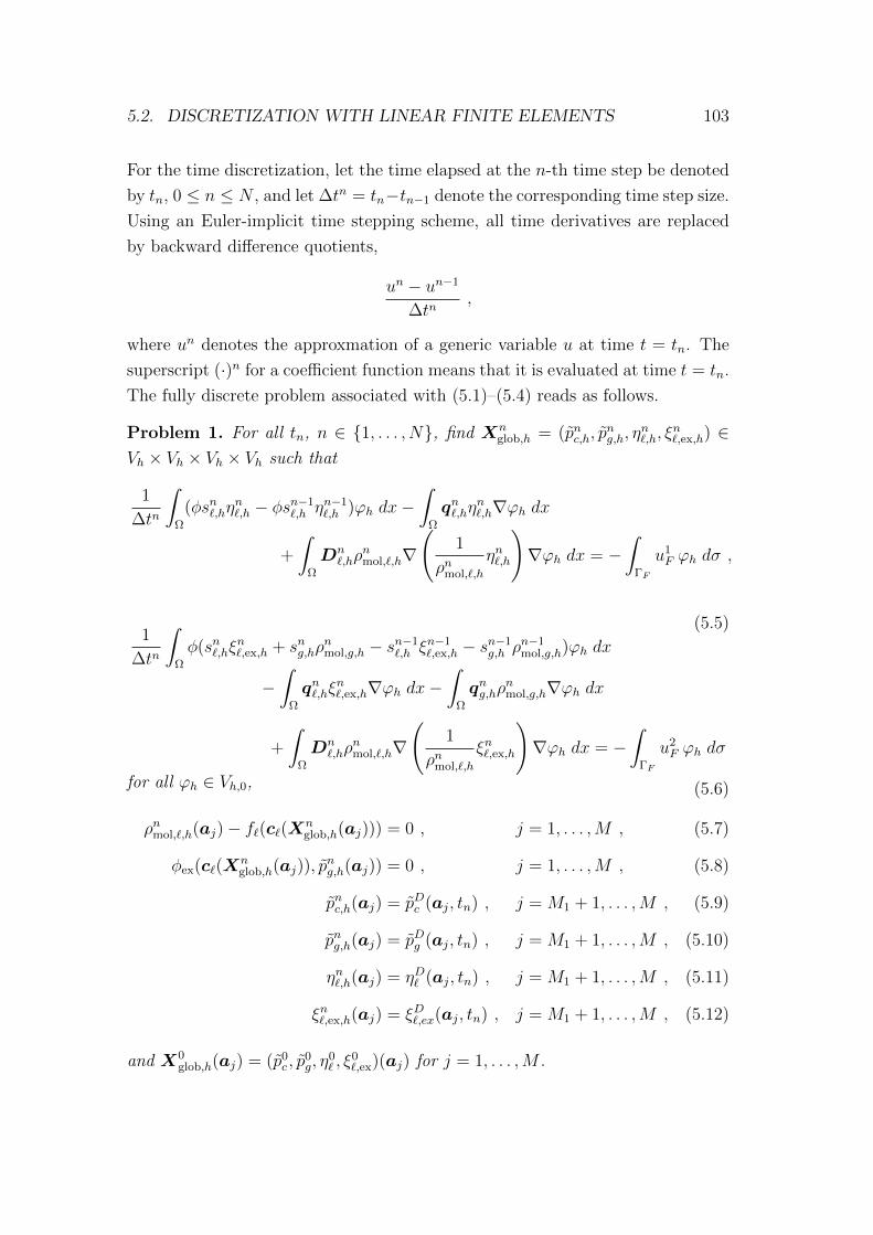
5.2. DISCRETIZATION WITH LINEAR FINITE ELEMENTS 103
For the time discretization, let the time elapsed at the n-th time step be denoted
by tn, 0 ≤ n ≤ N , and let ∆tn = tn−tn−1 denote the corresponding time step size.
Using an Euler-implicit time stepping scheme, all time derivatives are replaced
by backward difference quotients,
un − un−1
∆tn,
where un denotes the approxmation of a generic variable u at time t = tn. The
superscript (·)n for a coefficient function means that it is evaluated at time t = tn.
The fully discrete problem associated with (5.1)–(5.4) reads as follows.
Problem 1. For all tn, n ∈ 1, . . . , N, find Xnglob,h = (pnc,h, p
ng,h, η
n`,h, ξ
n`,ex,h) ∈
Vh × Vh × Vh × Vh such that
1
∆tn
∫Ω
(φsn`,hηn`,h − φsn−1
`,h ηn−1`,h )ϕh dx−
∫Ω
qn`,hηn`,h∇ϕh dx
+
∫Ω
Dn`,hρ
nmol,`,h∇
(1
ρnmol,`,h
ηn`,h
)∇ϕh dx = −
∫ΓF
u1F ϕh dσ ,
(5.5)1
∆tn
∫Ω
φ(sn`,hξn`,ex,h + sng,hρ
nmol,g,h − sn−1
`,h ξn−1`,ex,h − sn−1
g,h ρn−1mol,g,h)ϕh dx
−∫
Ω
qn`,hξn`,ex,h∇ϕh dx−
∫Ω
qng,hρnmol,g,h∇ϕh dx
+
∫Ω
Dn`,hρ
nmol,`,h∇
(1
ρnmol,`,h
ξn`,ex,h
)∇ϕh dx = −
∫ΓF
u2F ϕh dσ
(5.6)for all ϕh ∈ Vh,0,
ρnmol,`,h(aj)− f`(c`(Xnglob,h(aj))) = 0 , j = 1, . . . ,M , (5.7)
φex(c`(Xnglob,h(aj)), p
ng,h(aj)) = 0 , j = 1, . . . ,M , (5.8)
pnc,h(aj) = pDc (aj, tn) , j = M1 + 1, . . . ,M , (5.9)
png,h(aj) = pDg (aj, tn) , j = M1 + 1, . . . ,M , (5.10)
ηn`,h(aj) = ηD` (aj, tn) , j = M1 + 1, . . . ,M , (5.11)
ξn`,ex,h(aj) = ξD`,ex(aj, tn) , j = M1 + 1, . . . ,M , (5.12)
and X0glob,h(aj) = (p0
c , p0g, η
0` , ξ
0`,ex)(aj) for j = 1, . . . ,M .

104 CHAPTER 5. DISCRETIZATION
Here, the secondary variables are defined in terms of the primary variables by
pn`,h(x) =M∑j=1
p`(Xnglob,h(aj))ϕj(x) ,
snα,h(x) =M∑j=1
sα(Xnglob,h(aj))ϕj(x) , α ∈ `, g ,
ρnmol/mass,α(x) =M∑j=1
ρmol/mass,α(Xnglob,h(aj))ϕj(x) , α ∈ `, g ,
where (p`, sα, ρmol/mass,α)(·) denotes the resolution function. The discrete diffusive
and advective fluxes are given by
qnα,h(x) = −K(x)krα(snα,h(x))
µα(∇pnα,h(x)− ρnmass,α,h(x) g) , (5.13)
Dn`,h(x) = αT |qn`,h(x)|I + (αL − αT )
qn`,h(x)⊗ qn`,h(x)
|qn`,h(x)| + φ43 sn`,h(x)
103 Ddiff,`I .
(5.14)
Finally, by expanding the global unknowns in terms of the basis functions of Vh,
pnc,h =M∑j=1
pnc,jϕj , png,h =M∑j=1
png,jϕj , ηn`,h =M∑j=1
ηn`,jϕj , ξn`,ex,h =M∑j=1
ξn`,ex,jϕj ,
and using the basis functions ϕj, j ∈ 1, . . . ,M1 of Vh,0 as test functions
in (5.5)–(5.6), a nonlinear system of equations for the unknowns Xnglob,j :=
(pnc,j, png,j, η
n`,j, ξ
n`,ex,j), j ∈ 1, . . . ,M1, is obtained in each time step.
Integrals of the form ∫Ω
ϕi(x)ϕj(x) dx ,
and integrals resulting from sources and sinks are discretized with the help of
mass lumping, using a quadrature of the form
I(f) =M∑i=1
ωif(ai) .

5.3. FV STABILIZATION 105
b
b
b
b
b
b
b
b
b
b
b
aj
Ωj
Figure 5.1: Control volume Ωj associated with aj
5.3 Finite volume stabilization for advection–
dominated problems
When advective transport dominates diffusion, the scheme (5.5)–(5.6) produces
numerical solutions containing unphysical oscillations. To tackle this problem, a
stabilization technique proposed in [Hof10] (see also [BFK14]) was implemented,
where the advective terms in (5.5)–(5.6) are discretized by finite volumes. In
the following, this stabilization is presented for the case that the underlying
discretization is the linear finite element method on triangles, cf. Section 5.2.
It should be noted, however, that it is also applicable for bilinear elements on
rectangles and for linear/bilinear elements on tetrahedral/hexahedral meshes in
three space dimensions, respectively. Given a conforming triangulation Th of Ω, a
dual grid is defined by connecting all edge midpoints of all triangles T ∈ Th with
the barycenter of the associated triangle. Thus, a control volume Ωj is generated
around each node aj, cf. Figure 5.1. The family of control volumes obtained by
this construction is called Donald diagram.

106 CHAPTER 5. DISCRETIZATION
The FV stabilization is based on the approximations∫Ω
∇ · (qn`,hηn`,h)ϕj dx ≈∫
Ωj
∇ · (qn`,hηn`,h) dx =
∫∂Ωj
(qn`,hηn`,h) · n∂Ωj dσ ,∫
Ω
∇ · (qng,hρnmol,g,h)ϕj dx ≈∫
Ωj
∇ · (qng,hρnmol,g,h) dx =
∫∂Ωj
(qng,hρnmol,g,h) · n∂Ωj dσ ,
where n∂Ωj denotes the outer unit normal vector of ∂Ωj. It consists in treating
the boundary integrals on the right hand side with an upwind-weighted finite
volume method. The integral∫∂Ωj
(qn`,hηn`,h) · n∂Ωj dσ =
∑T∈Th
∫∂Ωj∩T
(qn`,hηn`,h) · n∂Ωj dσ
is approximated by (see Figure 5.2 for the used notation)∫∂Ωj∩T
(qn`,hηn`,h) · n∂Ωj dσ ≈ qn`,h((a0 + ac)/2) · n[a0,ac](r01η
n`,h(a0)
+ (1− r01)ηn`,h(a1)) + qn`,h((ac + a2)/2) · n[ac,a2](r02ηn`,h(a0) + (1− r02)ηn`,h(a2)) ,
where the normals n[a0,ac] and n[ac,a2] have the length |a0 − ac| and |ac − a2|,respectively. The integral∫
∂Ωj
(qng,hρnmol,g,h) · n∂Ωj dσ =
∑T∈Th
∫∂Ωj∩T
(qng,hρnmol,g,h) · n∂Ωj dσ
is treated analogously. For the weights r01 and r02, there exist different ap-
proaches. For example, the choice r01 = r02 = 0.5 corresponds to a central
scheme, which is not suitable for advection–dominated problems. A full upwind
scheme is obtained for
r01 =
1 if qn`,h((a0 + ac)/2) · n[a0,ac] ≥ 0 ,
0 otherwise ,
r02 =
1 if qn`,h((ac + a2)/2) · n[ac,a2] ≥ 0 ,
0 otherwise .
In contrast to the upwind stabilization used in [Hof10], our upwind scheme is

5.3. FV STABILIZATION 107
b
b
b
b
b
b
Ωj ∩ T
a2
a0
a1
a0
ac
a1
a2
n[ac,a2]
n[a0,ac]
Figure 5.2: Intersection of a control volume Ωj with a triangle T
fully nonlinear since the velocities qn`,h and qng,h depend nonlinearly on the phase
pressures, saturations and mass densities, which themselves are nonlinear func-
tions of the primary variables pnc,h, png,h, η
n`,h and ξn`,ex,h by means of the resolution
function and (5.13).
For simple model problems involving a linear transport operator and a scalar
diffusion coefficient which is piecewise constant, it can be shown that the full
upwind scheme is inverse monotone on grids that consist of nonobtuse triangles,
cf. [KA03, Theorem 6.19]. This means that monotonicity is preserved and that
overshoots and undershoots are prevented. In our numerical tests the full upwind
scheme worked well for the multiphase multicomponent model involving nonlinear
transport.
Since the the full upwind scheme introduces a significant amount of artificial
diffusion to the problem, resulting in a smearing of sharp fronts in the numerical
solution, it is recommended to use full upwinding only in those parts of the
domain where the PDEs are advection dominated. This can is accomplished
by using partial upwinding or exponential upwinding, where the upwind weights
depend on the local grid Peclet number, cf. [KA03].

108 CHAPTER 5. DISCRETIZATION
5.4 Implicit elimination
After the discretization in time and space, a nonlinear system of equations of the
form
Rn(Xnglob,h,Xloc(X
nglob,h)) = 0
remains to be solved in each time step, where Rn represents the residual function
associated with the discrete global problem and Xnglob,h denotes the vector of
global unknowns at time t = tn. As we solve this system using the (Semismooth)
Newton method, the derivative ∂Xloc
∂Xglobof the local variables with respect to the
global variables must be evaluated in each iteration step. If the resolution function
exists in an open neighborhood U of Xnglob,h, it satisfies
φloc(Xglob,Xloc(Xglob)) = 0 for all Xglob ∈ U ,
where φloc represents all local equations defining the resolution function. Then,
the implicit function theorem implies
∂φloc
∂Xglob
+∂φloc
∂Xloc
∂Xloc
∂Xglob
= 0 on U , (5.15)
which represents a linear system of equations for ∂Xloc
∂Xglob. Thus, despite of the
fact that an explicit representation of the resolution function is not available, its
derivative can be computed by solving (5.15). Note that in general, the resolution
function is only piecewise smooth, cf. Theorem 4.1.9. If it is not differentiable at
some point, an element of the B-subdifferential can be determined by replacing
φloc in (5.15) by one of its essentially active selection functions in that point, cf.
Lemma 4.1.5.
Let us now apply this approach to our problem. First, we make the approximation
DXglobξs,kin ≈ 0 . (5.16)
This assumption is justified since the variable ξs,kin corresponds to kinetic reac-
tions which proceed slowly compared to equilibrium reactions. Moreover, as the
local equations do not depend on ξ`,sorp and ξ`,min, cf. (3.74)–(3.84) and (3.41),
it holds that Dξ`,sorpXloc = 0 and Dξ`,minXloc = 0. Moreover, p` depends only on

5.4. IMPLICIT ELIMINATION 109
the global variables pg and pc by means of p` = pg− pc, which implies ∂p`∂pg
= 1 and∂p`∂pc
= −1. The remaining derivatives can be computed in five sequential steps:
(1) The variable sg depends only on the global variable pc, and we obtain the
explicit representation
∂sg∂pc
=
0 if pc ≤ pc(0) ,(∂pc∂sg
)−1
if pc > pc(0)
for the derivative of sg with respect to pc.
(2) The variables ηs depend only on pc by means of
ηs =1
s`(pc)s0`η
0s ,
cf. (3.75), where s0` and η0
s denote the initial values of s` and ηs, respec-
tively. This implies
∂ηs∂pc
=1
s2`
∂sg∂pc
s0`η
0s .
(3) The derivatives
∂(ξ`,mob, ξs,sorp, ξs,min)
∂(η`, ξ`,ex, ξ`,kin, ξsorp, ξmin)
can be computed by solving the linear systems
∂(φmob,φsorp,φmin)
∂(ξ`,mob, ξs,sorp, ξs,min)· ∂(ξ`,mob, ξs,sorp, ξs,min)
∂(η`, ξ`,ex, ξ`,kin, ξsorp, ξmin)
=∂(φmob,φsorp,φmin)
∂(η`, ξ`,ex, ξ`,kin, ξsorp, ξmin).
(5.17)
After possibly rearranging the equilibrium mineral reactions and the entries
of ξs,min with respect to the current mineral assemblage, specified by the
index sets A and I representing the active and inactive mineral reactions,
we obtain
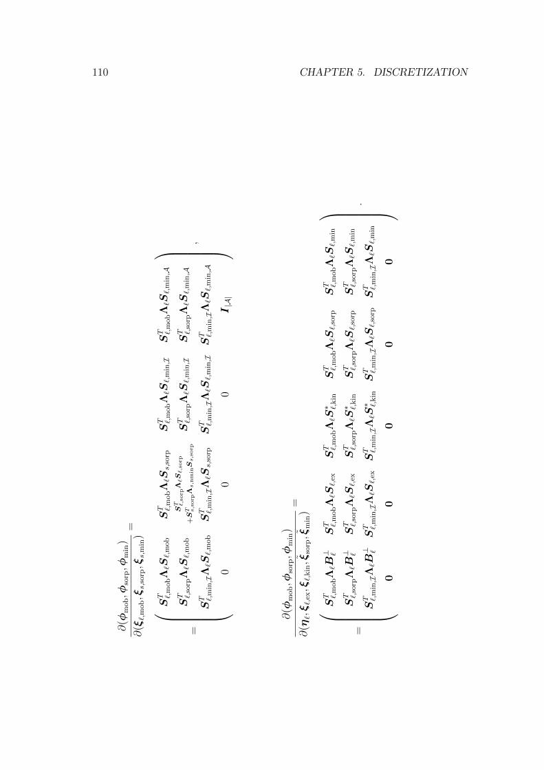
110 CHAPTER 5. DISCRETIZATION
∂(φ
mob,φ
sorp,φ
min
)
∂(ξ`,
mob,ξ
s,so
rp,ξ
s,m
in)
=
=
ST `,
mobΛ`S
`,m
ob
ST `,
mobΛ`S
s,so
rpST `,
mobΛ`S
`,m
in,I
ST `,
mobΛ`S
`,m
in,A
ST `,
sorp
Λ`S
`,m
ob
ST `,sorp
Λ`S`,sorp
+ST s,sorp
Λs,n
minSs,sorp
ST `,
sorp
Λ`S
`,m
in,I
ST `,
sorp
Λ`S
`,m
in,A
ST `,
min,I
Λ`S
`,m
ob
ST `,
min,I
Λ`S
s,so
rpST `,
min,I
Λ`S
`,m
in,IST `,
min,I
Λ`S
`,m
in,A
00
0I|A|
,
∂(φ
mob,φ
sorp,φ
min
)
∂(η
`,ξ`,
ex,ξ
`,kin,ξ
sorp,ξ
min
)=
=
ST `,
mobΛ`B⊥ `
ST `,
mobΛ`S
`,ex
ST `,
mobΛ`S∗ `,k
inST `,
mobΛ`S
`,so
rpST `,
mobΛ`S
`,m
in
ST `,
sorp
Λ`B⊥ `
ST `,
sorp
Λ`S
`,ex
ST `,
sorp
Λ`S∗ `,k
inST `,
sorp
Λ`S
`,so
rpST `,
sorp
Λ`S
`,m
in
ST `,
min,I
Λ`B⊥ `ST `,
min,I
Λ`S
`,ex
ST `,
min,I
Λ`S∗ `,k
inST `,
min,I
Λ`S
`,so
rpST `,
min,I
Λ`S
`,m
in
00
00
0
.

5.4. IMPLICIT ELIMINATION 111
Using the matrices
B =
S`,mob S`,sorp S`,min,I
0 Ss,sorp 0
, Λnmin =
Λ`
Λs,nmin
,
where Λ` and Λs,nmin are defined as in Section 4.1, the system matrix of
these linear systems can be rewritten as
∂(φmob,φsorp,φmin)
∂(ξ`,mob, ξs,sorp, ξs,min)=
BTΛnminB ∗
0 I |A|
.
Since the columns of B are linearly independent, the matrix BTΛnminB
is symmetric and positive definite. This implies that the above matrix is
regular and that the linear systems (5.17) are uniquely solvable. Note that
since the system matrix is the same for all right hand sides, the solutions of
these systems are obtained by computing an LU factorization of the matrix
and using backward/forward elimination for each right hand side.
(4) As soon as the systems (5.17) have been solved, the derivatives∂ξ`,mob
∂Xglob,
∂ξs,sorp∂Xglob
and∂ξs,min
∂Xglobcan be used to compute the derivatives of the concentra-
tions with respect to the global variables by means of
∂c`∂Xglob
= S`,glob +(S`,mob S`,sorp S`,min
)
∂ξ`,mob
∂Xglob
∂ξs,sorp∂Xglob
∂ξs,min
∂Xglob
,
∂cs,nmin
∂Xglob
= B⊥s
∂ηs∂Xglob
+ Ss,sorp
∂ξs,sorp
∂Xglob
,
∂cs,min
∂Xglob
=∂ξs,min
∂Xglob
,

112 CHAPTER 5. DISCRETIZATION
which is a consequence of the retransformation
c` = S`,globXglob + S`,locXloc ,
cs,nmin = Ss,locXloc ,
cs,min = ξs,min ,
cf. (3.41), and the approximation (5.16). Here, the block matrices S`,glob,S`,loc
and Ss,loc are defined by
S`,glob =(
0 0 B⊥` S`,ex 0 0 S∗`,kin S`,sorp S`,min
),
S`,loc =(
0 0 0 S`,mob S`,sorp S`,min 0 0 0 0 0),
Ss,loc =(
0 0 B⊥s 0 Ss,sorp 0 S∗s,kin 0 0 0 0
)and exhibit the same block structure as the global and local variables,
respectively, cf. (3.64).
(5) Finally, we obtain from (2.39), (2.40), (2.6) and the above considerations
that the derivatives of the molar and mass densities with respect to the
global variables have the representations
∂ρmol,g
∂Xglob
=∂fg∂pg
∂pg∂Xglob
,∂ρmass,g
∂Xglob
= M1 · ∂ρmol,g
∂Xglob
,
∂ρmass,`
∂Xglob
=
I∑i=1
M i ∂ci`∂Xglob
,∂ρmol,`
∂Xglob
=
I∑i=1
∂ci`∂Xglob
.

Chapter 6
The numerical framework
6.1 The M++ toolbox
The algorithms developed as a part of this thesis were implemented in M++, a
finite element toolbox for parallel computations based on C++ using the MPI
standard for parallelization, cf. [Wie, Wie05, Wie10]. It relies on data structures
for parallel computing which are directly linked to geometric quantities of an
underlying mesh, and which are adapted to the requirements of a general finite
element realization. More precisely, all geometric objects (cells, faces, edges)
are referenced by their midpoints, and all algebraic data structures (vectors and
matrices) are tied to the nodal points of the finite elements. Together, they build
Distributed Point Objects (DPO), where the parallel distribution of the grid is
made transparent by processor lists assigned to the points. All objects are stored
in hash tables (where the keys are points) so that pointers can be completely
avoided. The general concept is described in the paper [Wie10].
M++ provides basic functionality for solving finite element problems, e. g., iterative
linear solvers (GMRES, BiCGStab, QMRCGStab) and preconditioners (SSOR,
ILU). Moreover, different types of finite elements (linear, mixed, Crouzeix-Raviart
etc.) and output formats for visualization (vtk, gp) are supported.
Our code is written for problems in 2D and 3D on unstructured simplicial or
quadrilateral/hexahedral meshes. The coarse grid is specified in a text file con-
taining information on the grid topology and remains fixed throughout the com-
putation. By not incorporating grid adaptivity, M++ represents a compromise
113

114 CHAPTER 6. THE NUMERICAL FRAMEWORK
between flexibility, compactness of the code, and the requirements for an optimal
performance.
The user specifies the problem in a script file including information about the
finite element ansatz spaces that should be used, the linear and nonlinear solvers,
stopping criteria, discretization parameters etc. In our implementation, the num-
ber of chemical species and chemical reactions may be given in the script file,
and the transformation of the nonlinear system using the reduction scheme is
performed automatically. Consequently, an arbitrary number of chemical species
and reactions can be handled. The code comprises all techniques that are de-
scribed in the following section including cutting strategies, starting value search
for the local Newton iterations, and special numerical treatment of the local
systems.
6.2 Adaptive time stepping
Since for explicit time stepping schemes, very strict time step constraints may
apply as the result of a CFL condition, we use the backward Euler method for time
discretization, which provides good stability properties (B-stability, L-stability)
and enables the use of large time steps. As a consequence, a nonlinear system
of equations has to be solved in each time step using some fixed point method.
To ensure efficiency, we use a damped Newton’s method for linearization, which
converges quadratically if the residual function is sufficiently smooth and if the
initial guess of the iteration is located close enough to the solution. Typically,
this is the case if the time step size is sufficiently small. For very large time steps,
however, the starting value may not lie in the region of quadratic convergence,
and the Newton solver may not converge at all or need many steps until the
stopping criterion is satisfied. For this reason, we update the time step size after
each time step depending on the number of Newton iterations that were necessary
to solve the nonlinear problem of the previous time step. More precisely, after
each successful time step, the current time step size is multiplied with the factor
β =Number of global Newton steps
OptSteps,
where OptSteps is a user-defined value for the optimal number of Newton steps.
With this strategy, the number of Newton steps tries to level off at this value.

6.3. THE GLOBAL NEWTON SOLVER 115
β =Number of global Newton steps
OptSteps
∆t *= β
∆t > ∆tmaxTRUE FALSE
∆t = ∆tmax ∅
∆t < ∆tminTRUE FALSE
∆t = ∆tmin ∅
t+∆t > TendTRUE FALSE
∆t = Tend − t ∅
Figure 6.1: Update of the time step size
Additionally, a maximum and a minimum step size can be specified by the user.
The detailed instructions for updating the time step size after a successful time
step are given in Figure 6.1.
For some applications, the number of Newton steps can be significantly reduced
if a linear extrapolation of the values of the previous two time steps is used as
an initial guess instead of the value of the previous time step. The resulting time
stepping algorithm is illustrated in Figure 6.2.
6.3 The global Newton solver
In the implementation done for this work, a damped Newton’s method is used
to linearize the nonlinear discrete equations resulting from the global and the
local problems. More precisely, Armijo’s rule is is used as a line search strategy
when updating the Newton step. Note that by the definition of the Semismooth
Newton method, the Jacobian of any essentially active selection function can

116 CHAPTER 6. THE NUMERICAL FRAMEWORK
Initialize: Xglob = X0glob ; Xold
glob = Xglob ; t = 0 ; told = 0 ; tnew = ∆t ; tsteps = 0 ;
while t < Tend
Extrapolation of previous time steps
TRUE FALSE
∆Xglob = ∆tt−told
(Xoldglob −Xglob)
Xnewglob -= ∆Xglob
∅
Solve nonlinear problem at time tnew with the Semismooth Newton method
using Xnewglob as iteration variable
Newton iteration converged
TRUE FALSE
Update ∆t depending on number
of Newton steps, cf. Figure 6.1
tsteps += 1
Xoldglob = Xglob
Xglob = Xnewglob
told = t
t = tnew
tnew += ∆t
Reduce time step size for restart
of time step:
∆t *= 0.5
tnew -= ∆t
Xnewglob = Xglob
tsteps > max steps ∆t < ∆tmin
TRUE FALSE TRUE FALSE
Error: max. number
of time steps reached
BREAK
∅Error: ∆t < ∆tmin
BREAK ∅
Figure 6.2: The adaptive time stepping algorithm

6.3. THE GLOBAL NEWTON SOLVER 117
be taken if the residual function is not differentiable for some Newton iterate.
The detailed algorithm for the global Newton solver is summarized in Figure 6.3.
The update of the global Newton step requires some special treatment, which is
described in the following section.
Solve local problems to determine Xloc = Xloc(Xglob)
Calculate defect R = R(Xglob,Xloc)
d = ‖R‖
while stopping criterion not satisfied
Assemble Jacobian J
Calculate Newton update by solving the linear system
J∆Xglob = −R
Update Xglob and Xloc using the Newton update ∆Xglob
Calculate defect R = R(Xglob,Xloc)
j = 0
while j < maxLineSearchSteps
d1 = ‖R‖
d1 < d
TRUE FALSE
BREAK
∆Xglob *= 0.5
Update Xglob and Xloc using theupdate −∆Xglob
Calculate defect R = R(Xglob,Xloc)
j += 1
d = d1
Figure 6.3: The damped Newton algorithm
118 CHAPTER 6. THE NUMERICAL FRAMEWORK
6.4 Special numerical treatment
6.4.1 Updating the global Newton step
In the k-th step of the global Newton iteration, the local problems have to be
solved in each grid point to determine the local variables Xkloc = Xloc(X
kglob) as a
function of the global variables. This requires a suitable starting value Xk,0loc for
the local Newton iteration. It was reported in [Hof10] that after solving the η
problem, i. e., the linear subproblem that decouples from the rest of the system
after employing the reduction scheme, it may happen that the new η variables
together with the other transformed variables correspond to negative concentra-
tions. This is not admitted, however, since the logarithms of the concentrations
are used as unknowns for solving the local problems, cf. Section 6.4.3. Therefore,
a feasible starting value has to be searched for the local Newton iterations. In
our formulation, there is no decoupling of η equations, but it may still happen
that, after adding the Newton update ∆Xk−1glob , the new global variables
Xkglob = Xk−1
glob + ∆Xk−1glob
together with the local variables Xk−1loc = Xk−1,end
loc of the previous Newton step
(which represent a natural choice for the starting value Xk,0loc of the local Newton
iteration) correspond to negative concentrations according to the retransforma-
tion. One possible solution of this problem is to restart the global Newton step
and add only a part of the computed Newton update,
Xkglob = Xk−1
glob + τ∆Xk−1glob , τ ∈ (0, 1) .
If this is done globally, i. e., for all nodes, this corresponds to a damping of the
global Newton method. It is preferred, however, to modify the variables locally,
i. e., only in those nodes where the starting value is unfeasible. In our numerical
experiments, the number of these nodes was less than 1% of all nodes. Since we
have Xk−1,endloc = Xloc(X
k−1glob ), a feasible starting value will be recovered by this
strategy if τ is sufficiently small.
This approach has the drawback that the current iterate of the global Newton
iteration is modified, which may affect the speed of convergence of the method.
Another possible strategy is to modify only the local transformed concentration
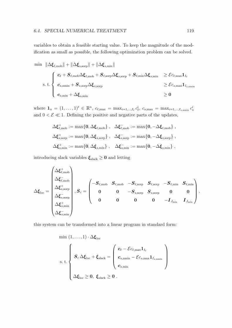
6.4. SPECIAL NUMERICAL TREATMENT 119
variables to obtain a feasible starting value. To keep the magnitude of the mod-
ification as small as possible, the following optimization problem can be solved.
min ‖∆ξ`,mob‖+ ‖∆ξs,sorp‖+ ‖∆ξs,min‖
s. t.
c` + S`,mob∆ξ`,mob + S`,sorp∆ξs,sorp + S`,min∆ξs,min ≥ Ec`,max1I`
cs,nmin + Ss,sorp∆ξs,sorp ≥ Ecs,max1Is,nmin
cs,min + ∆ξs,min ≥ 0
where 1n = (1, . . . , 1)t ∈ Rn, c`,max = maxi=1,...,I` ci`, cs,max = maxi=1,...,Is,nmin
cisand 0 < E 1. Defining the positive and negative parts of the updates,
∆ξ+`,mob := max0,∆ξ`,mob , ∆ξ−`,mob := max0,−∆ξ`,mob ,
∆ξ+s,sorp := max0,∆ξs,sorp , ∆ξ−s,sorp := max0,−∆ξs,sorp ,
∆ξ+s,min := max0,∆ξs,min , ∆ξ−s,min := max0,−∆ξs,min ,
introducing slack variables ξslack ≥ 0 and letting
∆ξloc =
∆ξ+`,mob
∆ξ−`,mob
∆ξ+s,sorp
∆ξ−s,sorp
∆ξ+s,min
∆ξ−s,min
,Sc =
−S`,mob S`,mob −S`,sorp S`,sorp −S`,min S`,min
0 0 −Ss,sorp Ss,sorp 0 0
0 0 0 0 −IJminIJmin
,
this system can be transformed into a linear program in standard form:
min (1, . . . , 1) ·∆ξloc
s. t.
Sc ∆ξloc + ξslack =
c` − Ec`,max1I`
cs,nmin − Ecs,max1Is,nmin
cs,min
∆ξloc ≥ 0, ξslack ≥ 0 .
120 CHAPTER 6. THE NUMERICAL FRAMEWORK
The variables c`, cs,nmin and cs,min are those (possibly negative) concentrations
that correspond to the current values of Xglob and Xloc according to the retrans-
formation. Since all entries in the vector (1, . . . , 1) are nonnegative, the simplex
tableau associated with the above linear program is dual feasible. Therefore, the
standard two-phase simplex method can be avoided and we are ready to start
with the dual simplex method.
Under the assumption that the local problem is solvable, its solution represents
a feasible starting value for the local problems. Then, if E is sufficiently small,
the above minimization problem admits a solution. On the other hand, if the
simplex method fails to converge, the set S defined in (4.10) is empty, and the
local problems are not solvable. In this case, the global Newton step has to be
modified. To overcome this problem, one could modify both the local and the
global variables with an update obtained from solving the extended minimization
problem
minεloc(‖∆ξ`,mob‖+ ‖∆ξs,sorp‖+ ‖∆ξs,min‖) + εglob(‖∆ξ`,ex‖+ ‖∆ξsorp‖
+ ‖∆ξmin‖+ ‖∆ξ`,kin‖+ ‖∆η`‖+ ‖∆ηs‖)
s. t.
c` + S`,ex∆ξ`,ex + S`,mob∆ξ`,mob + S`,sorp(∆ξsorp + ∆ξs,sorp)
+ S`,min(∆ξmin + ∆ξs,min) + S∗`,kin∆ξ`,kin +B⊥` ∆η` ≥ Ec`,max1I`
cs,nmin + Ss,sorp∆ξs,sorp + B⊥s ∆ηs ≥ Ecs,max1Is,nmin
cs,min + ∆ξs,min ≥ 0 ,
where we choose εglob εloc to ensure that the local variables are modified in
the first place.
Since these optimization problems are large and computationally expensive to
solve, we follow a different strategy that additionally tackles another problem that
may occur when the local problems are solved: even if a feasible starting value
is available or found during starting value search, it may happen that the local
Newton iteration fails to converge. One potential reason for this is that the global
Newton solver has reached an unphysical state where there exists no nonnegative
solution for the concentrations. In this case, it is inevitable to modify the global
Newton iterate, e. g., by taking only a part of the global Newton update. More
precisely, we employ a backtracking line search along the Newton update using

6.4. SPECIAL NUMERICAL TREATMENT 121
Armijo’s rule. Since the previous time step was successful, the local problems
will be solvable and the starting value search will converge if a sufficiently small
part of the full Newton update is used. Moreover, it should be noted that the
problem arises only in very few grid points. Hence, the convergence of the global
Newton method is hardly affected by this strategy. The resulting algorithm for
updating the global Newton step is summarized in Figure 6.4.
Xk+1glob = Xk
glob +∆Xkglob ; Xk+1,0
loc = Xk,endloc ; A = 0 ;
while A 6= 1
(cℓ, cs,nmin)(Xk+1glob ,X
k+1,0loc ) > 0
TRUE FALSE
Solve local problem with
starting value Xk+1,0loc
starting value search → ∆Xk+1loc
successful
NO YES
Xk+1,0loc += ∆Xk+1
loc
solve local problem with
starting value Xk+1,0loc
successful
YES NO
∆Xkglob*= 0.5
Xk+1glob
-= ∆Xkglob
Xk+1,0loc
-= ∆Xk+1loc
A = 1
converged
YES NO
A = 1 ∆Xkglob*= 0.5
Xk+1glob -= ∆Xk
glob
Figure 6.4: Algorithm for employing the global Newton update using startingvalue search
Instead of taking the valueXk,endloc as the initial value for solving the local problems
in the k + 1-th Newton step, an extrapolation based on a linearization of the
resolution function can be used:
Xk+1,0loc = Xk
loc +∂Xloc(X
kglob,X
kloc)
∂Xglob
·∆Xkglob .
Then, fewer steps are typically necessary to reach the stopping criterion of the

122 CHAPTER 6. THE NUMERICAL FRAMEWORK
local Newton iteration. On the other hand, our numerical experiments showed
that the number of grid points where starting value search is necessary increases
if this extrapolation is used. In our code, the use of the extrapolation is optional
and can be enabled/disabled in the script file.
6.4.2 Gas phase appearance and disappearance
−1.0 · 106
−0.80 · 106
−0.60 · 106
−0.40 · 106
−0.20 · 106
0.00 · 106
0.20 · 106
−1.0 · 1060 2 · 105 4 · 105 6 · 105 8 · 105 1060
time [years]
p c[Pa]
−1.0 · 106
−0.80 · 106
−0.60 · 106
−0.40 · 106
−1.0 · 1060 2 · 105 4 · 1050
Figure 6.5: Evolution of pc at Γin
One benefit of using pc as a global unknown is the fact that the saturations sg and
s` depend solely on that variable. This does not only simplify the evaluation of
the resolution function, but can be further exploited to improve the convergence
of the global Newton solver by employing a suitable cutting strategy when the
gas phase appears. The appearance of the gas phase in a grid point may cause
problems for the global Newton solver. Figure 6.5 shows the evolution of pc at
the inflow for the numerical example considered in Section 7.2 (hard test case).
Before the gas phase starts to appear, the variable pc increases almost linearly.
Once the gas phase has appeared, however, it remains approximately constant.
Therefore, in the vicinity of the the phase transition point, the Newton solver
may dramatically overestimate the update for pc, resulting in an unphysical jump
of the gas phase saturation from 0 to a value close to 1. As a consequence, very
small time steps may be required to reproduce the phase transition correctly

6.4. SPECIAL NUMERICAL TREATMENT 123
by the numerical solver. The cutting strategy proposed in [dC15] detects the
appearance of the gas phase by testing in each grid point and in every Newton
step if the entry pressure threshold has been succeeded (for the first time) by the
variable pc. If this is the case, it is manually set to a value closely above the entry
pressure. The positive impact of this cutting strategy on the convergence of the
global Newton solver was demonstrated in [dC15].
6.4.3 The local problems
The resolution function Xglob 7→ Xloc is evaluated numerically by solving the
algebraic equations (3.74)–(3.84) for the local unknowns. With our choice of
primary variables, this problem decomposes into smaller subproblems that can
be solved in several sequential steps.
(1) First, the variable sg is calculated from the equation (3.76). If the retention
curve sg 7→ pc(sg) admits an explicit inverse p−1c (this applies for the van
Genuchten–Mualem and the Brooks–Corey relations), we obtain
sg(pc) =
0 if pc ≤ pc(0) ,
p−1c (pc) if pc > pc(0) .
(2) As soon as the saturation s` = 1− sg is known, equation (3.75) can be used
to determine ηs explicitly by means of
ηs =1
s`(pc)s`(0)ηs(0) .
Note that this is always possible since our model excludes the case that the
liquid phase completely vanishes at any point of the domain.
124 CHAPTER 6. THE NUMERICAL FRAMEWORK
(3) In the next step, the nonlinear system
φmob(c`) = 0 , (6.1)
φsorp(c`, cs,nmin) = 0 , (6.2)
φmin(c`, cmin) = 0 , (6.3)
φ(s`ξs,kin − sold` ξ
olds,kin)
∆t= φs`As,kinRkin(c`, cs,nmin) (6.4)
is solved for the unknowns ξ`,mob, ξs,sorp, ξs,min and ξs,kin using Newton’s
method (see below). Afterwards, the concentrations c`, cs,nmin and cs,min
can be computed with the help of the retransformation (3.41).
(4) Finally, the defining equation of pc provides the liquid pressure,
p` = pg − pc ,
and the molar and mass densities are reconstructed from (3.81)–(3.84).
When the nonlinear system (6.1)–(6.4) is solved in terms of the transformed
variables, the linear systems arising in each Newton step may be ill-conditioned,
e. g., when the concentration values vary over a wide range of magnitudes. For this
reason, the logarithms of the variables should be used as unknowns. However, this
is not immediately possible since the equilibrium conditions contain the logarithm
of a sum, e. g.,
0 = Kmob + ST`,mob ln(c`) = Kmob + ST`,mob ln(S`,exξ`,ex + . . .+B⊥` η` ) .
To tackle this problem, the local problems are solved in terms of the concentra-
tions c` and cs instead of the transformed variables, cf. [Hof10]. If we replace the
transformed variables ξ`,mob, ξs,sorp and ξs,min by the concentrations, the number
of unknowns is increased by I`+Is−(Jmob +Jsorp +Jmin). Hence, additional equa-
tions are needed to close the system. Therefore, the defining equations for the
global variables η`, ηs, ξ`,ex, ξ`,kin, ξs,kin, ξsorp and ξmin are added to (6.1)–(6.4).

6.4. SPECIAL NUMERICAL TREATMENT 125
Indeed, the number of these defining equations is
I` − (Jex + Jmob + Jsorp + Jmin + J∗`,kin) + Is − (Jsorp + Jmin + J∗s,kin)
+ Jex + Jsorp + Jmin + J∗`,kin + J∗s,kin
= I` + Is − Jmob − Jsorp − Jmin ,
which corresponds to the number of additional unknowns. Then, in the local
problems, the variables c`, cs and ξs,kin are determined by solving the extended
system
φmob(c`) = 0 ,
φsorp(c`, cs,nmin) = 0 ,
φmin(c`, cs,min) = 0 ,
η` = (S⊥`TB⊥` )−1S⊥`
Tc`
ηs = (S⊥sTB⊥s )−1S⊥s
Tcs
ξ`,ex =((BT
` S∗`)−1BT
` c`)i=1,...,Jex
ξ`,kin =((BT
` S∗`)−1BT
` c`)i=Jeq+1,...,Jeq+J∗`,kin
ξsorp =((BT
` S∗`)−1BT
` c`)i=Jex+Jmob+1,...,Jex+Jmob+Jsorp
−((BT
s S∗s)−1BT
s cs)i=1,...,Jsorp
ξmin =((BT
` S∗`)−1BT
` c`)i=Jex+Jmob+Jsorp+1,...,Jeq
− cs,min
ξs,kin =((BT
s S∗s)−1BT
s cs)i=Jsorp+Jmin+1,...,Jsorp+Jmin+J∗s,kin
φ(s`ξs,kin − sold` ξ
olds,kin)
∆t= φs`As,kinRkin(c`, cs,nmin) .
Now, the logarithms of the concentrations can be used as unknowns in the equi-
librium laws. Defining l` := ln(c`) and ls,nmin := ln(cnmin), the system translates

126 CHAPTER 6. THE NUMERICAL FRAMEWORK
into
φmob(l`) = 0 , (6.5)
φsorp(l`, ls,nmin) = 0 , (6.6)
φmin(l`, cs,min) = 0 , (6.7)
η` = (S⊥`TB⊥` )−1S⊥`
Texp(l`) (6.8)
ηs = (S⊥sTB⊥s )−1S⊥s
T(
exp(ls,nmin)cs,min
)(6.9)
ξ`,ex =((BT
` S∗`)−1BT
` exp(l`))i=1,...,Jex
(6.10)
ξ`,kin =((BT
` S∗`)−1BT
` exp(l`))i=Jeq+1,...,Jeq+J∗`,kin
(6.11)
ξsorp =((BT
` S∗`)−1BT
` exp(l`))i=Jex+Jmob+1,...,Jex+Jmob+Jsorp
−(
(BTs S∗s)−1BT
s
(exp(ls,nmin)cs,min
))i=1,...,Jsorp
(6.12)
ξmin =((BT
` S∗`)−1BT
` exp(l`))i=Jex+Jmob+Jsorp+1,...,Jeq
− cs,min
(6.13)
ξs,kin =(
(BTs S∗s)−1BT
s
(exp(ls,nmin)cs,min
))i=Jsorp+Jmin+1,...,Jsorp+Jmin+J∗s,kin
(6.14)
φ(s`ξs,kin − sold` ξ
olds,kin)
∆t= φs`As,kinRkin(exp(l`), exp(ls,nmin)) (6.15)
Note that due to the structure of S∗s and Bs, the variables ηs, ξs,kin and ξsorp do
not depend on cs,min, cf. (3.6) and (3.9). Consequently, the variable cs,min appears
only in the blocks (6.7) and (6.13). It was shown in [Hof10] that this fact can be
exploited to further reduce the system by eliminating the concentrations cs,min
and reconstructing them according to the explicit representation of (6.13) (in the
case that the mineral is present) or by setting cks,min = 0 (if it is not present).
Accordingly, either the k-th equation of block (6.13) or the k-th equation of block
(6.7) can be omitted. This is possible as long as each mineral concentration occurs
only once in the system (6.5)–(6.15). If kinetic mineral reactions are included
into the model, however, the mineral concentrations additionally occur in the

6.4. SPECIAL NUMERICAL TREATMENT 127
For each mineral reaction k
ϕmin,k(lℓ) > cmin,k
TRUE FALSE
A[k] = 0 A[k] = 1
cks,min = 0 ∅
Assemble local defect (6.5)–(6.15) without (6.7)
For each mineral reaction k
A[k]
0 1
def[Jmob + Jsorp + k] = ϕmin,k(lℓ)def[Jmob + Jsorp + k] = 0
Figure 6.6: Detailed algorithm for assembling the local defect
terms resulting from the discretization of their time derivative, cf. Section 6.4.4.
Therefore, the above elimination is no longer possible. Since the code written for
this thesis includes the case of kinetic mineral reactions, the full system (6.5)–
(6.15) is solved.
When the defect of the system (6.5)–(6.15) is calculated, it must be checked for
each mineral reaction whether the corresponding mineral is present in the next
iteration step or not. If the minimum in (2.33) is attained in the first argument,
the mineral will be present, whereas if it is attained in the second argument, it
will not be present. In the code written as part of this work, the result is stored
in a vector A, where A[k] = 1 corresponds to the case that the k-th mineral is
present and A[k] = 0 means that it is absent. The algorithm for calculating the
local defect is summarized in Figure 6.6. After solving the system (6.5)–(6.15),
the transformed variables ξ`,mob and ξs,sorp are calculated with the help of their
definitions
ξ`,mob =((BT
` S∗`)−1BT
` c`)i=Jex+1,...,Jex+Jmob
, ξs,sorp =((BT
s S∗s)−1BT
s cs)i=1,...,Jsorp
,

128 CHAPTER 6. THE NUMERICAL FRAMEWORK
and the transformed variable ξs,min is equal to cs,min. It should be noted, however,
that ξ`,mob is not needed to assemble the defect associated with the global system
(3.65)–(3.73).
When the system (6.5)–(6.15) is solved using Newton’s method, it may happen
that the Jacobian becomes numerically singular. This is the case if a global
variable is defined as a linear combination of concentrations where all coefficients
have the same sign, and if the value of this variable is close to zero. This is because
it holds that ∂ exp(l`)∂l`
= exp(l`) = c`, i. e., the line in the Jacobian corresponding
to the defining equation of this global variable has entries that are close to zero.
Following [Hof10], we do not solve the linear system J∆x = d to compute the
Newton update ∆x, but the minimization problem (assume for a moment that
J ∈ R(n,n),d ∈ Rn)
Minimize ‖∆x‖22 on
L(d) := z ∈ Rn : ‖Jz − d‖22 ≤ ‖Jy − d‖2
2 for all y ∈ Rn .
This problem admits a unique solution which can be computed with the help
of a QR factorization for rank-deficient matrices. If column pivoting is applied,
the rows of the Jacobian that are numerically singular are detected, and it is
ensured that an error is introduced only in those equations associated with these
rows, i. e., all other equations are solved exactly. The order of magnitude of the
total error that is created by solving the minimization problem instead of the
linear system lies in the range of the machine precision. The detailed algorithm
is described in [Hof10].
6.4.4 Kinetic mineral reactions
Kinetic reactions involving minerals require some special treatment since pure
solids are typically assumed to have constant activity. Consequently, if the mass
action law is used to model the rate function of a kinetic mineral reaction, the
reaction rate does not depend on the concentration of the associated mineral.
This is in contrast to the kinetic reactions between nonminerals considered in
Section 2.3.1. Consider, for example, the reaction
A+ 2B ←→M ,

6.4. SPECIAL NUMERICAL TREATMENT 129
where A and B represent two components of the liquid phase, and M is a mineral.
The reaction rate according to the mass action law is given by
R(cA` , cB` ) = kfc
A` (cB` )2 − kb , (6.16)
where cA` and cB` denote the concentrations of A and B in the liquid phase.
Assuming that there is no gas phase, the equations describing the evolution of
the concentrations of A, B and M read
∂t(φcA` ) + L`cA` = −φR(cA` , c
B` ) ,
∂t(φcB` ) + L`cB` = −2φR(cA` , c
B` ) ,
∂t(φcMs ) = φR(cA` , c
B` ) .
Obviously, the rate law (6.16) cannot be valid in the case that
cMs = 0 ∧ kfcA` (cB` )2 − kb < 0 ,
since a negative rate R would imply a negative mineral concentration cMs . A well-
known strategy to comply with the nonnegativity of the mineral concentration
is the use of a set valued rate function, cf. [vDK97, vDKS98, KvDH95, vDP04].
For the above example, this approach reads
∂t(φcMs ) = φ(kfc
A` (cB` )2 − wkb) , (6.17)
w ∈ H(cMs ) , (6.18)
where H denotes the set-valued Heaviside “function”,
H(u) =
1 if u > 0 ,
[0, 1] if u = 0 ,
0 if u < 0 .

130 CHAPTER 6. THE NUMERICAL FRAMEWORK
In [Hof10], a complementarity approach was proposed to treat kinetic mineral
reactions, which reads
cMs (∂t(φcMs )− φ(kfc
A` (cB` )2 − kb)) = 0 , (6.19)
cMs ≥ 0 , ∂t(φcMs )− φ(kfc
A` (cB` )2 − kb) ≥ 0 . (6.20)
It can be shown that the weak formulations of (6.17)–(6.18) and of (6.19)–(6.20)
are equivalent, cf. [Hof10, Theorem 5.2]. While the first one is well suited for the-
oretical considerations, the complementarity approach is preferred for numerical
computations since it admits an equivalent reformulation as an equation using
the minimum function,
mincMs , ∂t(φcMs )− φ(kfcA` (cB` )2 − kb) = 0 .
The complementarity approach ensures the nonnegativity of the mineral concen-
tration, and it does not require a regularization parameter, which is typically
used to discretize problems involving set-valued functions, see, e. g., [DPvDC08].
In the following, it is shown how the complementarity approach can be incor-
porated into our model. If cjs,min represents the j-th mineral and if this mineral
participates in a kinetic mineral reaction, the equation describing the evolution
of cjs,min reads
φmin,j(c`, cjs,min) := mincjs,min, ∂t(φs`c
js,min)− φs`Rmin,j(c`) = 0 , (6.21)
where Rmin,j denotes the reaction rate depending on the concentrations of the
components of the liquid phase,
Rmin,j(c`) = kf,j
I∏i=1sij<0
ai(c)−sij − kb,j
I∏i=1sij>0
ai(c)+sij .
In its fully discrete form, (6.21) yields a nonlinear algebraic equation that can be
treated in the same way as the equilibrium conditions resulting from equilibrium
reactions. More precisely, if the j-th mineral reaction is kinetic, (6.21) it is incor-
porated as the j-th equation in the block (3.79) of algebraic equations associated
with equilibrium minerals, which is in contrast to the kinetic reactions without
minerals, the rates of which appear on the right hand side of (3.66)–(3.69).

Chapter 7
Numerical results
7.1 The MoMaS benchmark on multiphase flow
In the first numerical example, we consider a benchmark problem related to the
migration of hydrogen in geological formations, which are discussed as potential
storage sites for radioactive waste. The storage concept is based on the presence of
multiple barriers that ensure storage security. On the one hand, there is the deep
rock environment which is required to be stable, low permeable and unaffected by
environmental change for a long time period (hundreds of thousands of years). On
the other hand, there are engineered barriers like the container of the radioactive
material, or a buffer or backfill material filling the space between the container
and the rock. One potential risk of this storage option is the generation of
highly explosive hydrogen gas due to corrosion, and a pressure buildup. As a
consequence, the engineered barriers or even the host rock may be perturbed,
and the waste material may be released.
The MoMaS benchmark on multiphase flow [MoM10, BGS13] was proposed in
order to improve the simulation of hydrogen migration in deep geological nuclear
waste storage sites. We recompute here the first test case which addresses the
problem of gas phase appearance and disappearance during a long-term injec-
tion process of hydrogen into a homogeneous and low-permeable porous medium.
The computational domain Ω is a rectangle of length 200m and width 20m, cf.
Figure 7.1. The domain is initially fully saturated with water, and hydrogen is
injected through the left part of the domain for a time period of Tinj = 5 · 105
131

132 CHAPTER 7. NUMERICAL RESULTS
Γin ΓD
Γimp
Γimp
Ω
Figure 7.1: Computational domain for the MoMaS benchmark problem
years. Since gravity is neglected, the problem is a pseudo 1D problem.
7.1.1 Parameters and setup
The hydrogen migration is driven by a two-phase two-component model, where
the first component is water and the second component is pure hydrogen. The
liquid phase may contain water and hydrogen, whereas the gas phase consists
only of hydrogen. We converted the benchmark description to match the formu-
lation in this work. In particular, molar concentrations are used instead of mass
concentrations.
Governing equations
The governing equations of the benchmark are
∂t(φs`c2`) + L`c2
` = 0 , (7.1)
∂t(φs`c1` + φsgρmol,g) + L`c1
` + Lgρmol,g = 0 , (7.2)
where c1` represents the molar concentration of hydrogen and c2
` is the molar
concentration of water in the liquid phase. The variable transformation for this
system was presented in Section 3.4.4 and yields the transformed variables η1` = c2
`
and ξ1`,ex = c1
` . If we use pc and ξ1`,ex as primary unknowns, our formulation
corresponds well to one of the formulations proposed in [NBI13] for the special
case of two-phase two-component flow.

7.1. THE MOMAS BENCHMARK ON MULTIPHASE FLOW 133
Initial and boundary conditions
Initially, the domain is liquid-saturated, and there is no hydrogen dissolved in
the liquid phase. Accordingly, the initial conditions read
p`(·, 0) = p0` , c1
`(·, 0) = 0 .
Note that the initial and boundary conditions must be converted to the specific
choice of primary variables used by our code. In this work, the extended pressure
pc and the transformed variable ξ1`,ex = c1
` were used as primary unknowns, and
were initialized by the values pc(·, 0) = −p0` and ξ1
`,ex(·, 0) = 0.
Denoting the hydrogen total flux and the water total flux by
Q1 = c1`q` + ρmol,gqg + j1
` , Q2 = c2`q` + j2
` ,
respectively, the following boundary conditions are imposed on ∂Ω = Γin∪ΓD∪Γimp:
1. No-flux on Γimp:
Q1 · n = 0 , Q2 · n = 0 ,
where n denotes the outer unit normal vector of Γimp.
2. Hydrogen injection on Γin:
Q2 · n = 0 , and Q1 · n =
q1in if t ≤ Tinj ,
0 otherwise .
3. Pure liquid water and a fixed pressure on ΓD:
p` = p`,out , c1` = 0 .
Closure relationships
Let us now choose the solubility function φex and phase compressibility laws f`
and fg consistently with the benchmark description. The hydrogen interphase

134 CHAPTER 7. NUMERICAL RESULTS
mass exchange follows Henry’s law, which is represented by the choice
φex(c`, pg) := Hpg − c1` .
For the compressibility laws, we set
f`(c`) := c1` + c2,std
` , (7.3)
fg(pg) :=pgRT
, (7.4)
where c2,std` denotes the molar density of water at standard conditions, T is the
(constant) temperature and R the universal gas constant. Note that (7.3) and
the constraint ρmol,` = c1` + c2
` are consistent with the condition c2` = c2,std
` from
the benchmark description, i. e., the concentration of water in the liquid phase
remains constant. The diffusion–dispersion tensor reads
Diα = φs`D
idiff,αI .
Finally, the assumption
j1` + j2
` = 0
is used to express the water diffusive flux in terms of the hydrogen diffusive flux.
Hence, only the diffusion coefficient D1diff,` must be specified. Finally, capillary
pressure and relative permeabilities are given by the van Genuchten–Mualem
model, cf. (2.9)–(2.11). The parameters of this test case are listed in Table 7.1.
Note that the molar mass of water was incorrect in the benchmark description.
The physically correct value is 1.8 · 10−2 kg mol−1.
The computations were carried out on a rectangular grid consisting of 160×16 =
2560 squares. Figure 7.2 shows the evolution of the gas phase saturation and
the phase pressures at the left boundary over time. Initially, the domain is
fully water-saturated. During the first injection period, all injected hydrogen
dissolves into the liquid phase and is transported by advection and diffusion.
Meanwhile, the liquid pressure remains almost constant. At t ≈ 13000 years,
the gas phase starts to appear and the gas phase saturation and phase pressures
start to increase. Between 105 years and 5 · 105 years, hydrogen is still injected
and the gas phase saturation keeps growing, while the phase pressures start to
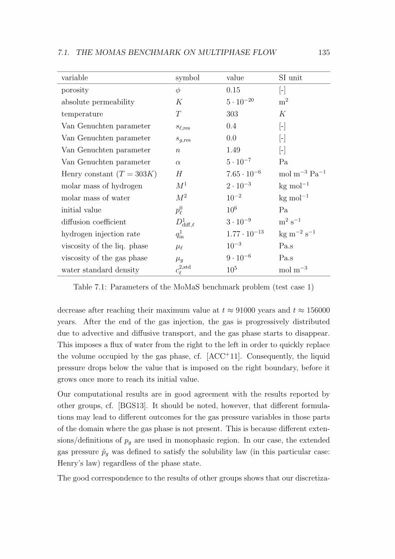
7.1. THE MOMAS BENCHMARK ON MULTIPHASE FLOW 135
variable symbol value SI unit
porosity φ 0.15 [-]
absolute permeability K 5 · 10−20 m2
temperature T 303 K
Van Genuchten parameter s`,res 0.4 [-]
Van Genuchten parameter sg,res 0.0 [-]
Van Genuchten parameter n 1.49 [-]
Van Genuchten parameter α 5 · 10−7 Pa
Henry constant (T = 303K) H 7.65 · 10−6 mol m−3 Pa−1
molar mass of hydrogen M1 2 · 10−3 kg mol−1
molar mass of water M2 10−2 kg mol−1
initial value p0` 106 Pa
diffusion coefficient D1diff,` 3 · 10−9 m2 s−1
hydrogen injection rate q1in 1.77 · 10−13 kg m−2 s−1
viscosity of the liq. phase µ` 10−3 Pa.s
viscosity of the gas phase µg 9 · 10−6 Pa.s
water standard density c2,std` 105 mol m−3
Table 7.1: Parameters of the MoMaS benchmark problem (test case 1)
decrease after reaching their maximum value at t ≈ 91000 years and t ≈ 156000
years. After the end of the gas injection, the gas is progressively distributed
due to advective and diffusive transport, and the gas phase starts to disappear.
This imposes a flux of water from the right to the left in order to quickly replace
the volume occupied by the gas phase, cf. [ACC+11]. Consequently, the liquid
pressure drops below the value that is imposed on the right boundary, before it
grows once more to reach its initial value.
Our computational results are in good agreement with the results reported by
other groups, cf. [BGS13]. It should be noted, however, that different formula-
tions may lead to different outcomes for the gas pressure variables in those parts
of the domain where the gas phase is not present. This is because different exten-
sions/definitions of pg are used in monophasic region. In our case, the extended
gas pressure pg was defined to satisfy the solubility law (in this particular case:
Henry’s law) regardless of the phase state.
The good correspondence to the results of other groups shows that our discretiza-

136 CHAPTER 7. NUMERICAL RESULTS
0.000
0.002
0.004
0.006
0.008
0.010
0.012
0.014
0.016
0.0000 2 · 105 4 · 105 6 · 105 8 · 105 1060
time [years]
saturation
[-]
0.000
0.002
0.004
0.006
0.008
0.010
0.012
0.014
0.016
0.0000 2 · 105 4 · 1050
sg
0.70 · 106
0.80 · 106
0.90 · 106
1.00 · 106
1.10 · 106
1.20 · 106
1.30 · 106
1.40 · 106
1.50 · 106
0.70 · 1060 2 · 105 4 · 105 6 · 105 8 · 105 1060
time [years]
pressure
[Pa]
0.70 · 106
0.80 · 106
0.90 · 106
1.00 · 106
1.10 · 106
0.70 · 1060 2 · 105 4 · 1050
pgpl
Figure 7.2: Evolution of gas phase saturation and pressures at Γin
tion and the code written in the framework of this thesis provide accurate results.
In particular, our formulation is capable of handling gas phase appearance and
disappearance. Although the two-phase two-component model studied in this
benchmark represents only a special case of the full reactive multiphase mul-
ticomponent model considered in this work, it contains all relevant transport
mechanisms of the full model.
7.1.2 Comparison of GIA and SIA
Since multiphase flow and multicomponent reactive transport models involve
large nonlinear and fully coupled systems of partial differential equations, ordi-
nary differential equations and algebraic equations, many codes utilize a splitting
approach to solve them numerically [HLL07, WF12, HSN12, XSS+12, AKV15].
Typically, the global problem is decomposed into a flow problem and a reactive
transport problem, which are solved sequentially. More precisely, in a first step,
pressures and saturations are determined as the solution of a two-phase two-
component flow problem for two dominant components (e. g., water and CO2),
neglecting the other components and their chemical reactions. In a second step,
the calculated pressures and the resulting Darcy velocities are used to update the
concentrations by solving a reactive transport problem. This approach is referred
to as sequential non-iterative approach (SNIA) or operator splitting. In doing so,
one can benefit from the availability of customized solvers for specific subprob-
lems, which can be easily coupled or combined. For example, the flow module

7.1. THE MOMAS BENCHMARK ON MULTIPHASE FLOW 137
PFLOW and the transport module PTRAN were merged into the multiphase
multicomponent reactive transport code PFLOTRAN, cf. [HLL07].
One drawback of SNIA is a splitting error, which may become large when the
physics are tightly coupled. Moreover, by neglecting chemical reactions of the
dominant components during the solution of the flow problem, an additional
modeling error is introduced. In the case of CO2 injection, this assumption may
not be justified since CO2 itself is reactive.
To eliminate the splitting error, the sequential iterative approach (SIA) can be
used, where the subproblems are solved alternately until they both converge
within prescribed tolerances. This may require many iterations in each time
step to meet the convergence criteria, in particular if fast kinetics and strong
chemical interactions are involved. When the iteration has converged, the solution
represents a solution of the global nonlinear problem.
While in the 1980s, Yeh and Tripathi [YT89] conclude that SIA is preferable,
the availability of increasing computational resources has attracted growing in-
terest in the global implicit approach for the simulation of reactive transport
problems during the past two decades [dDE10, AK10, KK05, KK07, Hof10]. In
the MoMaS benchmark on reactive transport, global methods proved to be very
competitive to other methods, and the code of Hoffmann et. al. showed equiv-
alent or lower CPU times than required by all other codes, cf. [CHK+10]. Very
recently, the global implicit approach has also been applied to coupled flow and
reactive transport problems, cf. [FDT12, SVG+13].
In this work, the global implicit approach is used, which means that all primary
variables are computed simultaneously during each time step by employing New-
ton’s method to the global system of nonlinear equations which results after the
model-preserving variable transformation has been employed. To demonstrate
that the resulting method is efficient and competitive to SIA, we recompute the
MoMaS benchmark problem from the previous section using SIA. For this pur-
pose, a sequential iterative approach is defined for the MoMaS benchmark by
decoupling the equations (7.1) and (7.2). More precisely, the k-th iteration step
associated with time step n (note that the index n and the discretization param-
eter h are omitted for a tighter notation) consists of two subproblems:

138 CHAPTER 7. NUMERICAL RESULTS
Subproblem 1
In the first step, the pressure variable pkc is determined by solving the equation
∂t(φs`c2`) + L`c2
` = 0 ,
where the secondary variables s`, c2` and p` (needed in the transport operator)
are expressed in terms of pkc with the help of the resolution function by means of
c2`(p
kc ) = c2,std
` ,
s`(pkc ) =
0 if pc < pc(0) ,
p−1c (pkc ) otherwise ,
p`(pkc ) =
c1,k−1`
H− pkc .
Subproblem 2
In the second step, pkc is known and c1,k` is determined by solving
∂t(φs`c1,k` + φsgρmol,g) + L`c1,k
` + Lgρmol,g = 0
with the secondary unknowns s`, sg, pg, ρmol,g and p` defined as
s` = s`(pkc ) , sg = 1− s` , pg(c
1,k` ) =
c1,k`
H,
ρmol,g(c1,k` ) =
c1,k`
HRT, p`(c
1,k` , pkc ) =
c1,k`
H− pkc .
The iteration is continued until the residuals corresponding to both equations
are within a given tolerance εabs for the pair (pkc , c1,k` ). Both subproblems are
treated fully implicitly, and the resulting nonlinear problems are linearized using
Newton’s method. In each time step, the time step size is adapted depending
on the total number N of Newton steps that were carried out in the previous
time step (summed over all iteration steps). More precisely, it is multiplied by
the factor N30
as long as the minimum/maximum time step size is not reached.
Moreover, the time step size is halved and the time step is repeated if the iteration
has not converged after 60 iteration steps. The detailed algorithm that is used
for the sequential iterative approach is illustrated in Figure 7.3. Since each of the

7.1. THE MOMAS BENCHMARK ON MULTIPHASE FLOW 139
subproblems consists only of one equation and is solved for one variable only, the
memory demand is clearly lower and the linear systems that have to be solved
are smaller than the linear systems resulting from the use of the global implicit
approach. Hence, the efficiency will be dominated by the number of iteration
steps that are necessary until both subproblems converge.
To compare the efficiency of SIA and GIA, the MoMaS benchmark is recomputed
using the same mesh as in the previous section and requiring an absolute tolerance
εabs to be reached by both methods. For GIA, pc and c1` are used as primary
variables. Moreover, the control parameter OptSteps=4 (cf. Section 6.2) is used
in the adaptive time stepping algorithm. The results of the performance test for
different values of εabs are displayed in Table 7.2, which shows the number of time
steps and the total number of Newton steps that were required by GIA and SIA
for different values of εabs. Obviously, the fixed point iteration of the sequential
approach converges slowly, resulting in rather poor convergence of SIA for strict
stopping criteria. This is due to a dramatic reduction of time step size by the
adaptive time stepper. On the other hand, for GIA, the global Newton method
converges quadratically and the time step size remains within a reasonable range
of values. The evolution of time step size for both approaches for εabs = 10−10
is illustrated in Figure 7.4. In this case, 15973 Newton steps were carried out by
the sequential approach for solving the subproblems 1 and 2, whereas only 409
Newton steps were necessary for the global implicit one. Although each Newton
step is computationally less expensive using SIA, the computation time was more
than ten times larger than the computation time of GIA. For more complex
problems involving chemical interactions, the difference in the performance of
the two methods is expected be even more significant. We conclude that the
global implicit approach represents an efficient and competitive way of solving
coupled flow and reactive transport problems, in particular if a high accuracy of
the nonlinear solver is required.

140 CHAPTER 7. NUMERICAL RESULTS
k = 0 , d1 = 99 , d2 = 99 , N = 0
while (d1 > εabs or d2 > εabs) and k < 60
k += 1
Solve Subproblem 1 for pk
N1 = Newton iterations required for subproblem 1
Solve Subproblem 2 for c1,kℓ
N2 = Newton iterations required for subproblem 2
N=N1 +N2
d1 = ‖Residual of Subproblem 1 for (pk, c1,kℓ )‖d2 = ‖Residual of Subproblem 2 for (pk, c1,kℓ )‖
d1 < εabs and d2 < εabs
TRUE FALSE
∆t *= N30 ∆t *= 0.5
Proceed to next time step Repeat time step
Figure 7.3: Schematic of the sequential iterative approach for the MoMaS bench-mark problem
0
1 · 1042 · 1043 · 1044 · 1045 · 1046 · 1047 · 1048 · 1049 · 10410 · 104
00 2 · 105 4 · 105 6 · 105 8 · 105 1060
time [years]
∆t[years]
GIASIA
0
1 · 1042 · 1043 · 1044 · 1045 · 1046 · 1047 · 1048 · 1049 · 10410 · 104
00 2 · 1050
b b bbbb b b b b b b b b b b b b b b b b b b b b b b b b b b b b b b b b b b b b b b b b b b b b
b b b b b b b b bb b b
bb b
b b
b
b
b
b
b
b b
b b b b b b b b b bb b b b
b b b b b b b b
b
b
b
b
b
b b bbb
b b b b b b b b b b b b b b b b b b b b b b b b b b b b b b b b b b b b b b b b b b b b b b b b b b b b b b b b b b b b b b b b b b b b b b b b b b b b b b b b b b b b b b b b b b b b b b b b b b b b b b b b b b b b b b b b b b b b b b b b b b b b b b b b b b b b b b b b b b b b b b b b b b b b b b b b b b b b b b b b b b b b b b b b b b b b b b b b b b b b b b b b b b b b b b b b b b b b b b b b b b b b b b b b b b b b b b b b b b b b b b b b b b b b b b b b b b b b b b b b b b b b b b b b b b b b b b b b b b b b b b b b b b b b b b b b b b b b b b b b b b b b b b b b b b b b b b b b b b b b b b b b b b b b b b b b b b b b b b b b b b b b b b b b b b b b b b b b b b b b b b b b b b b b b b b b b b b b b b b b b b b b b b b b b b b b b b b b b b b b b b b b b b b b b b b b b b b b bb b b b b b b b b b b b b b b b b b b
b b b b b b b b b b b b b b b b b b b b b b b b b b b b b b b bb b b b
b b b b b b b b b b b b b b b b b b b b b b b b b b b b b b b b b b b b b b b b b b b b b b b b bb b b b b b b b b b b b b b b
b b b b b b b b b
b
b
b
b b
b
Figure 7.4: Evolution of the time step size for SIA and GIA for εabs = 10−10

7.2. INFLUENCE OF DIFFERENT RETENTION CURVES 141
GIA SIA
εabs time st. Newton st. CPU time time st. Newton st. CPU time
10−5 54 206 4.3 min 46 1215 6.4 min
10−6 56 211 4.4 min 75 2060 10.9 min
10−7 67 260 5.9 min 118 3397 17.9 min
10−8 74 299 6.2 min 190 5550 29.5 min
10−9 89 351 7.1 min 324 9591 51.7 min
10−10 101 409 8.4 min 536 15973 86.6 min
Table 7.2: Performance of GIA and SIA for the MoMaS benchmark
7.2 Influence of different retention curves
The performance of the global numerical solver is strongly influenced by the soil
parameters of the problem. In the previous section, hydrogen injection into a very
dense and low-permeable material was simulated, which requires different soil pa-
rameters than CO2 injection into deep saline aquifers consisting of sandstone. To
investigate further the effect of different retention curves on the convergence of
the Newton solver, a simple modification of the MoMaS benchmark considered in
the previous section was proposed in [dC15]. The modified benchmark problem
involves two test cases using two different values of the van Genuchten param-
eter α in the definition of the capillary pressure–saturation curve: the value
α1 = 5 · 10−7 Pa was adopted from the MoMaS benchmark and corresponds to a
very low-permeable rock material, and α2 = 5 · 10−4 Pa represents a sandstone
aquifer. The resulting retention curves are shown in Figure 7.5.
Governing equations
The system is governed by the conservation equations (7.1)–(7.2), where diffusion
of component 1 (hydrogen) in the liquid phase is now expressed in terms of the
gradient of its molar concentration,
j1` = −D1
`∇c1` .

142 CHAPTER 7. NUMERICAL RESULTS
0.0 · 108
0.5 · 108
1.0 · 108
1.5 · 108
2.0 · 108
0.0 · 1080.0 0.2 0.4 0.6 0.8 1.00.0
effective liquid phase saturation Sℓ,e [-]
capillary
pressure
p c[Pa]
0.0 · 108
0.5 · 108
1.0 · 108
0.0 · 1080.0 0.2 0.40.0
α1 = 5 · 10−7
α2 = 5 · 10−4
Figure 7.5: Retention curves of the modified MoMaS benchmark problem
The diffusion-dispersion tensor of hydrogen in the liquid phase follows an ap-
proach of Jin and Jury [JJ96] and is given by
D1` = φ
43 s2`D
1diff,`I .
For the diffusive flux of water in the liquid phase, the relation j2` = −j1
` is used.
Initial and boundary conditions
The computational domain is initially liquid-saturated with no hydrogen being
dissolved in the liquid phase. The initial conditions read
p`(·, 0) = p0` , c1
`(·, 0) = 0 .
As in the MoMaS benchmark, hydrogen is injected through the left part of the
computational domain at a constant rate q1in at Γin. At Tinj = 5 · 105 years, the
injection is stopped and the simulation is continued until the final time Tend =
106 years. Accordingly, the the following boundary conditions are imposed on
∂Ω = Γin∪ΓD∪Γimp:

7.2. INFLUENCE OF DIFFERENT RETENTION CURVES 143
1. No-flux on Γimp:
Q1 · n = 0 , Q2 · n = 0 .
2. Hydrogen injection through Γin:
Q2 · n = 0 , Q1 · n =
q1in if t ≤ Tinj ,
0 otherwise .
3. Pure liquid water and a fixed liquid pressure on ΓD:
p` = p`,out , c1` = 0 .
The computational domain Ω = (0, 200) of this benchmark problem is one dimen-
sional, but since our code was written for 2D and 3D simulations, we consider it
as a pseudo 1D problem and run the computations on a thin stripe consisting of
N rectangles, cf. Figure 7.6. On the upper and lower boundary, no flux conditions
are imposed, and on the right boundary, Dirichlet conditions are imposed for c1`
and p`.
(0, 0) (200, 0)
(200, 1)(0, 1)
T1 T2 T2 TN. . .Γin ΓD
Γimp
Γimp
Figure 7.6: Computational mesh for the modified MoMaS benchmark problem
Closure relationships
For the hydrogen interphase mass exchange, Henry’s law is employed, i. e.,
φex(c`) := Hpg − c1` ,

144 CHAPTER 7. NUMERICAL RESULTS
and the compressibility laws are given by the functions
f`(c`) := c2,std` ,
fg(pg) :=pgRT
,
where the constant c2,std` denotes the molar density of water at standard condi-
tions. As a consequence, the liquid phase has constant molar concentration (but
varying mass density) in this example. All parameters associated with this test
problem are listed in Table 7.3. Since the simulation turned out to be much more
challenging using the parameter α2, we refer to this case as the “hard” test case,
whereas the use of the parameter α1 is referred to as the “easy” test case.
variable symbol value SI unit
porosity φ 0.15 [-]
absolute permeability K 5 · 10−20 m2
temperature T 303 K
Van Genuchten parameter s`,res 0.4 [-]
Van Genuchten parameter sg,res 0.0 [-]
Van Genuchten parameter n 1.49 [-]
Van Genuchten parameter α1 5 · 10−7 Pa
Van Genuchten parameter α2 5 · 10−4 Pa
Henry constant (T = 303K) H 7.65 · 10−6 mol m−3 Pa−1
molar mass of hydrogen M1 2.0 · 10−3 kg mol−1
molar mass of water M2 1.8 · 10−2 kg mol−1
initial value p0` 106 Pa
diffusion coefficient D2diff,` 3 · 10−9 m2 s−1
diffusion coefficient D1diff,g 0 m2 s−1
hydrogen injection rate q1in 1.77 · 10−13 kg m−2 s−1
viscosity of the liq. phase µ` 10−3 Pa.s
viscosity of the gas phase µg 9 · 10−6 Pa.s
standard water density c2,std` 55555.56 mol m−3
Table 7.3: Parameters of the modified benchmark problem

7.2. INFLUENCE OF DIFFERENT RETENTION CURVES 145
Grid convergence
A grid convergence study is carried out for both test cases. For this purpose, the
numerical solution of the problem is calculated on different levels of refinement,
where the number of rectangles in x direction is doubled in each refinement step,
resulting in a grid consisting of N = 100 · 2i cells on level i. As in the previous
section, pc and c1` are used as primary variables. Since an analytical solution of
the problem is not known, the solution on level i = 10 (N = 102400) is used as
a reference solution. It is illustrated in Figures 7.7, where the evolution of the
gas phase saturation and the evolution of the pressures at the inflow boundary
are shown. On each level of refinement, the experimental order of convergence is
determined by
EOCi+1 =1
log(2)| log
(eiei+1
)| ,
where ei denotes the L2 error between the solution on level i and the reference
solution. The relative L2 error ereli is defined as the ratio between ei and the L2
norm of the reference solution. All computations are run with a constant time
step size ∆t = 0.5 years, which is chosen sufficiently small to ensure that the
time discretization error is negligible compared to the space discretization error.
The results of the convergence study are listed in Tables 7.4 and 7.5. For the
easy test case, first order convergence is observed for the variables sg, p` and c1` ,
which is optimal for the upwind LFEM–FV scheme. For the hard test case, the
convergence rate is slightly lower for the variable sg. This is in accordance with
the results reported in [dC15].
Performance
In addition to the grid convergence study, this benchmark problem was proposed
to enable a comparison of the performance of different numerical solvers. For
that purpose, we recompute both test cases using the adaptive time stepping
strategy described in Section 6.2 and the control parameters of Table 7.6. In

146 CHAPTER 7. NUMERICAL RESULTS
0.000
0.005
0.010
0.015
0.020
0.0000 2 · 105 4 · 105 6 · 105 8 · 105 1060
time [years]
saturation
[-]
0.000
0.005
0.010
0.015
0.020
0.0000 2 · 105 4 · 1050
sg
0.70 · 106
0.80 · 106
0.90 · 106
1.00 · 106
1.10 · 106
1.20 · 106
1.30 · 106
1.40 · 106
1.50 · 106
0.70 · 1060 2 · 105 4 · 105 6 · 105 8 · 105 1060
time [years]
pressure
[Pa]
0.70 · 106
0.80 · 106
0.90 · 106
1.00 · 106
1.10 · 106
0.70 · 1060 2 · 105 4 · 1050
pgpℓ
0.00
0.02
0.04
0.06
0.08
0.10
0.000 2 · 105 4 · 105 6 · 105 8 · 105 1060
time [years]
saturation
[-]
0.00
0.02
0.04
0.000 2 · 105 4 · 1050
sg
0.70 · 106
0.80 · 106
0.90 · 106
1.00 · 106
1.10 · 106
1.20 · 106
1.30 · 106
1.40 · 106
1.50 · 106
0.70 · 1060 2 · 105 4 · 105 6 · 105 8 · 105 1060
time [years]
pressure
[Pa]
0.70 · 106
0.80 · 106
0.90 · 106
1.00 · 106
1.10 · 106
0.70 · 1060 2 · 105 4 · 1050
pgpℓ
Figure 7.7: Evolution of gas phase saturation and pressures at Γin for the easytest case (top) and the hard test case (bottom)
sg p` c1`
i N ereli EOCi erel
i EOCi ereli EOCi
0 100 1.78e-02 3.26e-04 9.02e-03
1 200 9.21e-03 0.95 1.92e-04 0.77 4.66e-03 0.95
2 400 4.67e-03 0.98 9.18e-05 1.06 2.36e-03 0.98
3 800 2.35e-03 0.99 4.74e-05 0.95 1.18e-03 0.99
4 1600 1.16e-03 1.01 2.31e-05 1.04 5.97e-04 0.99
5 3200 5.70e-04 1.03 1.13e-05 1.03 2.98e-04 1.00
6 6400 2.80e-04 1.03 5.61e-06 1.01 1.41e-04 1.08
7 12800 1.31e-04 1.10 2.62e-06 1.10 6.58e-05 1.10
Table 7.4: Relative L2-errors and experimental orders of convergence (EOC) forthe easy test case (α1 = 5 · 10−7) at t = 105 years.

7.2. INFLUENCE OF DIFFERENT RETENTION CURVES 147
sg p` c1`
i N ereli EOCi erel
i EOCi ereli EOCi
0 100 7.72e-2 1.68e-03 2.99e-02
1 200 4.88e-2 0.66 1.13e-03 0.57 1.71e-02 0.81
2 400 3.16e-2 0.63 5.82e-04 0.95 9.64e-03 0.82
3 800 2.11e-2 0.59 3.33e-04 0.81 5.33e-03 0.85
4 1600 1.38e-2 0.60 1.94e-04 0.78 2.89e-03 0.88
5 3200 8.97e-3 0.63 1.12e-04 0.80 1.52e-03 0.93
6 6400 5.50e-3 0.70 5.37e-05 1.06 7.71e-04 0.98
7 12800 3.15e-3 0.80 2.64e-05 1.03 3.72e-04 1.05
Table 7.5: Relative L2-errors and experimental orders of convergence (EOC) forthe hard test case (α2 = 5 · 10−4) at t = 105 years.
Tables 7.7 and 7.8, we list the number of time steps and Newton iterations (suc-
cessful and failed) that were necessary to compute the numerical solution on
different levels of refinement. For these computations, the linear extrapolation
of the previous time steps described in Section 6.2 was disabled and the value of
the previous time step was used as an initial guess for the global Newton method
at each time step.
Clearly, a significant higher number of Newton steps is required for the hard
test case than for the easy test case. More precisely, the number of Newton
steps almost doubles in each refinement step for the hard test case, whereas it
remains approximately constant for the easy test case. This is in accordance
with the results reported by R. de Cuveland and P. Bastian from the University
of Heidelberg [dC15], cf. Tables 7.9 and 7.10 . They use capillary pressure and
gas pressure as primary unknowns and discretize the equations with an Euler-
implicit cell-centered finite volume scheme. The nonlinear systems of equations
are solved with an inexact Newton method using the same stopping criterion as
in this work.
Although we solved a 2D problem with approximately twice as many unknowns as
for the corresponding 1D problem, our solver needed fewer time steps and Newton
iterations on all refinement levels. One of the reasons for this might be the fact
that we use the analytical Jacobian in our Newton method. Thus, no numerical
differentiation is required, which may lead to inaccurate approximations of the

148 CHAPTER 7. NUMERICAL RESULTS
control parameter value
εrel 10−6
εabs 0.0
max. line search steps 3
max. Newton iterations 30
∆tmin 1 year
∆tmax 106 years
OptSteps 10
Table 7.6: Control parameters for the performance test
Jacobian. Moreover, our time stepping algorithm and line search strategy is
different from the ones used in [dC15], which may have a strong impact on the
global performance. The choice of primary variables, however, seems to have
only little influence on the performance for this test problem. In further numerical
tests, we obtained the identical number of time steps and Newton iterations using
p` instead if pc or using pg instead of c1` = ξ1
`,ex.
We conclude this section by noting that our solver provides an accurate and
efficient numerical scheme which proved to be competitive to other fully implicit
solvers for the two-phase two-component model considered in this and in the
previous section.
N unknowns time steps (failed) Newton steps
100 404 21 (2) 153
200 804 20 (1) 144
400 1604 18 (3) 123
800 3204 29 (9) 246
1600 64042 31 (12) 253
3200 12804 32 (13) 263
Table 7.7: Benchmark performance results for the easy test case (α1 = 5 · 10−4)

7.2. INFLUENCE OF DIFFERENT RETENTION CURVES 149
N unknowns time steps (failed) Newton steps
100 404 93 (11) 994
200 804 167 (25) 1756
400 1604 273 (46) 3060
800 3204 454 (64) 4932
1600 6404 883 (166) 9659
3200 12804 1490 (380) 16626
Table 7.8: Benchmark performance results for the hard test case (α2 = 5 · 10−4)
N time steps (failed) Newton steps (failed)
100 48 (7) 309 (70)
200 62 (11) 422 (110)
400 76 (15) 511 (150)
800 89 (18) 630 (180)
160 92 (19) 643 (190)
3200 89 (18) 629 (180)
Table 7.9: Computational results reported by Uni Heidelberg (R. de Cuvelandand P. Bastian) for the easy test case (α1 = 5 · 10−7)
N time steps (failed) Newton steps (failed)
100 213 (55) 1335 (550)
200 403 (107) 2641 (1070)
400 781 (206) 5535 (2060)
800 1477 (390) 10701 (3990)
1600 2827 (746) 20751 (7440)
3200 5488 (1441) 38942 (13699)
Table 7.10: Computational results reported by Uni Heidelberg (R. de Cuvelandand P. Bastian) for the hard test case (α2 = 5 · 10−4)
150 CHAPTER 7. NUMERICAL RESULTS
7.3 CO2 sequestration
In this section, we consider the injection of CO2 into a deep aquifer covered by
an impermeable layer of rock for the purpose of permanent geological seques-
tration. This is considered as a promising approach to reduce the emission of
greenhouse gases into the atmosphere. The storage concept is based on different
trapping mechanisms that prevent the injected CO2 from being released into the
atmosphere.
Typically, CO2 is injected in its supercritical state where it adopts properties
midway between a gas and a liquid. More precisely, it has the low viscosity of
a gas and the high density of a liquid. Consequently, the ideal gas law used for
hydrogen injection is not applicable for carbon sequestration. Instead, we employ
the EOS of Duan [DMW92] to compute the density of CO2, cf. Figure 7.8.
When CO2 dissolves into the liquid phase, it causes density variations of the liquid
phase that may influence the flow regime. According to experimental data, the
density of aqueous solutions of CO2 can be as much as 2-3% higher than that of
pure water, which triggers downward migration due to gravitational forces. We
use the approach of Garcia [Gar01] to define the function f` that represents the
molar liquid phase density.
Regarding the solubility of CO2 in water, Henry’s law, which was used in the
previous numerical examples, is invalid at the high pressure conditions prevailing
at a deep underground CO2 storage site. We use the EOS of Spycher and Pruess
[SP05] to define the function φex representing the interphase mass exchange of
CO2. Figure 7.9 shows the solubility curves of CO2 in water for different tem-
peratures, neglecting salinity and the presence of other components in the liq-
uid phase. For temperatures below the critical temperature (Tcrit = 304.15K),
the curves exhibit a non-differentiable kink at the transition point between the
gaseous and liquid phase state. For the viscosity of the gas phase, an approach
of Fenghour et al. [FWV98] is used, cf. Figure 7.10.
Since the coefficient functions described above are given only implicitly, their
evaluation may be computationally expensive. Therefore, lookup tables are ini-
tially generated and cubic splines are used to evaluate the coefficient functions
and their derivatives during the simulation.

7.3. CO2 SEQUESTRATION 151
0
200
400
600
800
1000
1200
00 1 · 107 2 · 107 3 · 107 4 · 107 5 · 107 6 · 1070
pg [Pa]
ρmass,g[kg/m
3]
0
200
400
600
800
1000
1200
00 1 · 107 2 · 107 3 · 1070
283.15 K293.15 K303.15 K313.15 K323.15 K
Figure 7.8: Mass density of CO2 as a function of pressure
0.000
0.005
0.010
0.015
0.020
0.025
0.030
0.035
0.040
0.0000 1 · 107 2 · 107 3 · 107 4 · 107 5 · 107 6 · 1070
pg [Pa]
CO
2molefraction
χ1 ℓ[m
ol/m
ol]
0.000
0.005
0.010
0.015
0.020
0.025
0.030
0.035
0.040
0.0000 1 · 107 2 · 107 3 · 1070
283.15 K293.15 K303.15 K313.15 K323.15 K
Figure 7.9: Solubility of CO2 as a function of pressure
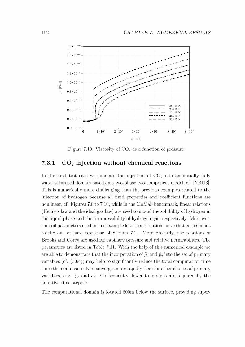
152 CHAPTER 7. NUMERICAL RESULTS
0.0 · 10−4
0.2 · 10−4
0.4 · 10−4
0.6 · 10−4
0.8 · 10−4
1.0 · 10−4
1.2 · 10−4
1.4 · 10−4
1.6 · 10−4
1.8 · 10−4
0.0 · 10−4
0 1 · 107 2 · 107 3 · 107 4 · 107 5 · 107 6 · 1070
pg [Pa]
µg[Pa·s
]
0.0 · 10−4
0.2 · 10−4
0.4 · 10−4
0.6 · 10−4
0.8 · 10−4
1.0 · 10−4
1.2 · 10−4
1.4 · 10−4
1.6 · 10−4
1.8 · 10−4
0.0 · 10−4
0 1 · 107 2 · 107 3 · 107 4 · 107 5 · 107 6 · 1070
283.15 K293.15 K303.15 K313.15 K323.15 K
Figure 7.10: Viscosity of CO2 as a function of pressure
7.3.1 CO2 injection without chemical reactions
In the next test case we simulate the injection of CO2 into an initially fully
water saturated domain based on a two-phase two-component model, cf. [NBI13].
This is numerically more challenging than the previous examples related to the
injection of hydrogen because all fluid properties and coefficient functions are
nonlinear, cf. Figures 7.8 to 7.10, while in the MoMaS benchmark, linear relations
(Henry’s law and the ideal gas law) are used to model the solubility of hydrogen in
the liquid phase and the compressibility of hydrogen gas, respectively. Moreover,
the soil parameters used in this example lead to a retention curve that corresponds
to the one of hard test case of Section 7.2. More precisely, the relations of
Brooks and Corey are used for capillary pressure and relative permeabilites. The
parameters are listed in Table 7.11. With the help of this numerical example we
are able to demonstrate that the incorporation of pc and pg into the set of primary
variables (cf. (3.64)) may help to significantly reduce the total computation time
since the nonlinear solver converges more rapidly than for other choices of primary
variables, e. g., pc and c1` . Consequently, fewer time steps are required by the
adaptive time stepper.
The computational domain is located 800m below the surface, providing super-

7.3. CO2 SEQUESTRATION 153
Γin
ΓimpΓD
Γimp
Γimp
Ω
10m
90m
600m
Figure 7.11: Computational domain for the CO2 injection scenario
critical conditions for the CO2 that is injected through the lower left part of the
domain at a constant rate q1in, cf. Figure 7.11.
Governing equations
The system is governed by the conservation equations (7.1)–(7.2), where compo-
nent 1 represents CO2 and component 2 represents water. Diffusion is expressed
in terms of the gradients of the molar fractions, cf. (2.4). Dispersion is not con-
sidered in this example, and molecular diffusion follows an approach of Millington
and Quirk [MQ61], resulting in the representation
Dα = φ43 s
103α Ddiff,αI (7.5)
for the diffusion-dispersion tensor.
Initial and boundary conditions
At the initial time, the domain is fully liquid-saturated with no CO2 being dis-
solved in the liquid phase. The initial conditions read
p`(·, 0) = p0` , c1
`(·, 0) = 0 ,
where
p0`(x, y) = 105 + (900− y)ρstd
mass,` · 9.81 Pa

154 CHAPTER 7. NUMERICAL RESULTS
represents hydrostatic pressure conditions in the domain. Here, ρstdmass,` denotes
the mass density of pure water.
The following boundary conditions are imposed on ∂Ω = Γin∪ΓD∪Γimp:
1. No-flux on Γimp:
Q1 · n = 0 , Q2 · n = 0 .
2. CO2 injection through Γin:
Q2 · n = 0 and Q1 · n = q1in .
3. Pure liquid water and hydrostatic pressure conditions on ΓD:
p` = p0` , c1
` = 0 .
variable symbol value SI unit
porosity φ 0.2 [-]
absolute permeability K 10−12 m2
temperature T 313.15 K
Brooks–Corey parameter s`,res 0.0 [-]
Brooks–Corey parameter sg,res 0.0 [-]
Brooks–Corey parameter λ 2.0 [-]
Brooks–Corey parameter pentry 1000 Pa
molar mass of CO2 M1 4.4 · 10−2 kg mol−1
molar mass of water M2 1.8 · 10−2 kg mol−1
pure water mass density (T = 313.15K) ρstdmass,` 992 kg m−3
diffusion coefficient Ddiff,` 2 · 10−9 m2 s−1
CO2 injection rate q1in 4 · 10−2 kg m−2 s−1
viscosity of the liq. phase (T = 313.15K) µ` 6.526 · 10−4 Pa.s
Table 7.11: Parameters for the CO2 injection scenario

7.3. CO2 SEQUESTRATION 155
Primary variables pc and pg Primary variables pc and c1`
cells time steps CPU time [s] time steps CPU time [s]
150 · 41 748 23 671 33
150 · 42 752 111 1600 270
150 · 43 2169 1559 4645 3469
150 · 44 6354 23323 13606 56695
Table 7.12: Comparison of two different choices of primary variables for the CO2
injection scenario
Comparison of different choices of primary variables
The numerical results are illustrated in Figure 7.12. Each of the graphics shows
the gas phase saturation at a specific point in time, calculated on a grid consisting
of 38400 rectangles. The computations were done in parallel on 20 processors.
Shortly after the injection of CO2 commences, a gas phase starts to appear and,
due to gravitational forces, propagates upwards. At the same time, the CO2
spreads in horizontal direction and finally accumulates below the upper boundary,
which is impermeable. To study the influence of the selected primary variables,
the computations were done for two different choices of primary variables, using
the same control parameters for the nonlinear and linear solvers. The number of
total time steps (successful and unsuccessful) and the computation time required
to reach the final simulation time Tend = 65 days are listed in Table 7.12. Clearly,
the use of two pressures pc and pg leads to a significant lower number of time steps
and CPU time than the use of pc along with the concentration c1` . This is because
the nonlinear solver converges more rapidly for the first choice, resulting in larger
time steps due to the adaptive time step control. There are two possible reasons
for this behavior: first, the coefficient functions presented above are functions
of pg and depend directly on a primary variable if the first formulation is used.
Secondly, the use of pc and pg implies that the gradient terms in the transport
operators depend linearly on the primary variables,
q` = −K kr`µ`
(∇(pg − pc︸ ︷︷ ︸=p`
)− ρmass,` g) , qg = −K krgµg
(∇pg − ρmass,g g) .

156 CHAPTER 7. NUMERICAL RESULTS
Figure 7.12: Gas phase saturation during the CO2 injection process after 7, 20and 65 days
If the same test is carried out for the MoMaS benchmark, the same number of
time steps is required for both formulations since Henry’s law implies c1` = Hpg,
i. e., both formulations translate into each other by linear rescaling of the primary
variables.
The above results motivate the incorporation of pc and pg into our global set of
primary variables for the general multiphase multicomponent model, cf. (3.64).
Although pg could be treated as a local variable by removing (3.73) from the set
of global equations, the formulation with both pressures was more efficient due
to the better convergence of the nonlinear solver for that case, despite of the fact
that the resulting linear systems are larger.

7.3. CO2 SEQUESTRATION 157
7.3.2 CO2 injection with chemical reactions
During the past years, the injection of CO2 into the subsurface with the goal
of reducing greenhouse gas emissions into the atmosphere has attracted wide
interest. A desirable effect in the geologic sequestration of CO2 would be if the
carbon precipitates forming minerals, which will effectively bind it to the rock
and thus permit a long-term storage. The desired mechanism is modeled by the
following set of generic chemical reactions (cf. [Kra08]):
CO(g)2
R1←→ CO(`)2
CO(`)2 + H2O
R2←→ HCO−3 + H+
Calcite + H+ R3←→ Ca2+ + HCO−3
Min A + 3H+ R4←→ Me3+ + SiO2
Min B + 2H+ R5←→ Me3+ + HCO−3
The reaction system consists of three minerals (Min A, Min B and calcite) and
seven aqueous reacting species, including water. The first reaction represents the
interphase mass exchange of CO2 between the gas and the liquid phase. The
second and the third reaction allow a transition of liquid CO2 into HCO−3 and
calcite. They both affect and are affected by the pH, i. e., the concentration of
H+. If a silicate (Min A) is present at the initial state, it dissolves at high H+
concentrations, releasing metal ions by reaction R4. Finally, the metal ions can
initiate the precipitation of Min B, trapping the carbon as a carbonate mineral.
Defining the concentration vectors
c` = (c1` , . . . , c
7`)T := (c
CO(`)2
` , cH2O` , c
HCO−3` , cH+
` , cCa2+
` , cMe3+
` , cSiO2` )T ,
cs = (c1s, c
2s, c
3s)T := (ccalcite
s , cMin As , cMin B
s )T ,

158 CHAPTER 7. NUMERICAL RESULTS
the stoichiometric matrix associated with this order of the chemical species reads
S =
Sg,eq
S`,eq
Ss,eq
=
−1 0 0
S`,ex S`,mob S`,min
0 0 IJmin
=
−1 0 0 0 0
1 −1 0 0 0
0 −1 0 0 0
0 1 −1 0 −1
0 1 1 3 2
0 0 −1 0 0
0 0 0 −1 −1
0 0 0 −1 0
0 0 1 0 0
0 0 0 1 0
0 0 0 0 1
.
The columns of this matrix and of its submatrices satisfy the linear indepen-
dence assumptions of Section 3.1, such that the reduction scheme can be applied.
Defining
S∗` =
1 −1 −1 0 0
0 −1 0 0 0
0 1 −1 0 −1
0 1 0 3 2
0 0 −1 0 0
0 0 0 −1 −1
0 0 0 −1 0
, S⊥` =
1
39
0 0
15 9
9 8
6 1
−3 −7
3 −6
15 9
,

7.3. CO2 SEQUESTRATION 159
we obtain the transformed variables
η` = (η1` , η
2` )T = (S⊥`
TS⊥` )−1S⊥`
Tc` =
0 1 0 1 1 2 1
0 0 1 −1 −2 −3 0
c1`
c2`
...
c7`
,
and
ξ` = (ξ`,ex, ξ`,mob, ξ1`,min, ξ
2`,min, ξ
3`,min)T
= (S∗`TS∗`)
−1S∗`Tc` =
1
39
39 −24 9 6 −3 3 15
0 −24 9 6 −3 3 15
0 −3 −7 4 −28 15 −3
0 15 9 6 −3 3 −24
0 −12 −15 3 18 −18 27
c1`
c2`
...
c6`
c7`
.
For this example, the system (3.65)–(3.73) is solved numerically with the trans-
formed variables as defined above. The diffusive fluxes are given by (2.4) using
the Bear–Scheidegger diffusion–dispersion tensor, cf. (2.5). For relative perme-
abilities and capillary pressure, we use the Brooks–Corey parametrizations. All
parameters are listed in Table 7.13. For the mass density, the solubility and the
viscosity of CO2 we use the same coefficient functions as in the previous section,
cf. Figures 7.8–7.10. All reactions are assumed at equilibrium with R1 being
governed by the solubility law and R2–R5 by the equilibrium mass action law.
The solubility products of these reactions are
cHCO−3` cH+
`
cCO
(`)2
`
= 10−3 ,cH+
`
cHCO−3` cCa2+
`
= 1 if ccalcites > 0 ,
(cH+
` )3
cMe3+
` cSiO2`
= 10−3 if cMin As > 0 ,
(cH+
` )2
cHCO−3` cMe3+
`
= 0.8 if cMin Bs > 0 ,
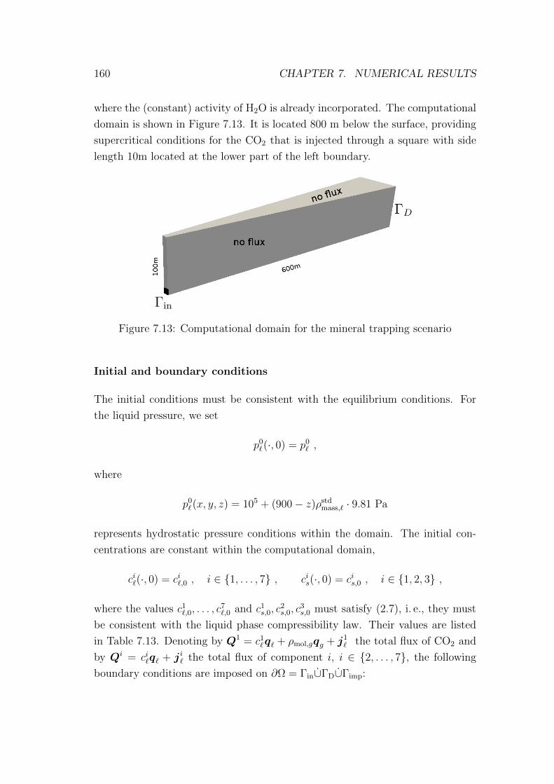
160 CHAPTER 7. NUMERICAL RESULTS
where the (constant) activity of H2O is already incorporated. The computational
domain is shown in Figure 7.13. It is located 800 m below the surface, providing
supercritical conditions for the CO2 that is injected through a square with side
length 10m located at the lower part of the left boundary.
Figure 7.13: Computational domain for the mineral trapping scenario
Initial and boundary conditions
The initial conditions must be consistent with the equilibrium conditions. For
the liquid pressure, we set
p0`(·, 0) = p0
` ,
where
p0`(x, y, z) = 105 + (900− z)ρstd
mass,` · 9.81 Pa
represents hydrostatic pressure conditions within the domain. The initial con-
centrations are constant within the computational domain,
ci`(·, 0) = ci`,0 , i ∈ 1, . . . , 7 , cis(·, 0) = cis,0 , i ∈ 1, 2, 3 ,
where the values c1`,0, . . . , c
7`,0 and c1
s,0, c2s,0, c
3s,0 must satisfy (2.7), i. e., they must
be consistent with the liquid phase compressibility law. Their values are listed
in Table 7.13. Denoting by Q1 = c1`q` + ρmol,gqg + j1
` the total flux of CO2 and
by Qi = ci`q` + ji` the total flux of component i, i ∈ 2, . . . , 7, the following
boundary conditions are imposed on ∂Ω = Γin∪ΓD∪Γimp:

7.3. CO2 SEQUESTRATION 161
1. No-flux conditions on ∂Ω \ (ΓD ∪ Γin) for all components:
Qi` · n = 0 , i ∈ 1, . . . , 7 .
2. CO2 injection through Γin:
Q1 · n = q1in , Qi · n = 0 , i ∈ 2, . . . , 7 .
3. The Dirichlet values prescribed at ΓD for the pressures and the concentra-
tions coincide with the initial values:
p` = p0` , ci` = ci`,0 , i ∈ 1, . . . , 7 .
The boundary and initial values for all other variables are induced by the variable
transformation and the resolution function.
Numerical results
The numerical results obtained on a grid consisting of 40960 hexahedra are shown
in Figures 7.14–7.16. Shortly after the injection of CO2 has started, a gas phase
appears, which continuously moves upwards due to gravity and accumulates be-
low the impermeable upper boundary. The CO2 that has dissolved into the liquid
phase causes the pH to decrease, inducing the dissolution of calcite and Min A.
Thereby, metal ions and bicarbonate are released, which initiates the precipita-
tion of Min B.
The propagation of the concentration fronts, in particular the appearance of the
gas phase and the precipitation and dissolution of minerals are well reproduced
by our solver. The computations were carried out using a maximum time step
size ∆tmax = 5000s and the control parameter OptSteps=6 for the time step
adaption. With these parameters, 2742 time steps (including 667 unsuccessful
ones) were carried out to simulate a time span of 85 days with an average number
of 4.32 Newton steps per time step.

162 CHAPTER 7. NUMERICAL RESULTS
variable symbol value SI unit
porosity φ 0.2 [-]
absolute permeability K 10−12 m2
temperature T 313.15 K
Brooks–Corey parameter s`,res 0.0 [-]
Brooks–Corey parameter sg,res 0.0 [-]
Brooks–Corey parameter λ 2.0 [-]
Brooks–Corey parameter pentry 1000 Pa
molar mass of CO2 M1 4.4 · 10−2 kg mol−1
molar mass of water M2 1.8 · 10−2 kg mol−1
molar mass of bicarbonate M3 6.1 · 10−2 kg mol−1
molar mass of hydrogen M4 10−3 kg mol−1
molar mass of calcium M5 4 · 10−2 kg mol−1
molar mass of metal ions M6 1.5 · 10−2 kg mol−1
molar mass of silicon dioxide M7 6 · 10−2 kg mol−1
initial concentration of CO2 c1`,0 10−2 kg m−3 mol−1
initial concentration of water c2`,0 55333.33 kg m−3 mol−1
initial concentration of bicarbonate c3`,0 10−2 kg m−3 mol−1
initial concentration of hydrogen c4`,0 10−3 kg m−3 mol−1
initial concentration of calcium c5`,0 10−1 kg m−3 mol−1
initial concentration of metal ions c6`,0 10−4 kg m−3 mol−1
initial concentration of silicon dioxide c7`,0 10−2 kg m−3 mol−1
initial concentration of calcite c1s,0 0.1 kg m−3 mol−1
initial concentration of Min A c2s,0 0.2 kg m−3 mol−1
initial concentration of Min B c3s,0 0.0 kg m−3 mol−1
pure water mass density (T = 313.15K) ρstdmass,` 992 kg m−3
diffusion coefficient D` 2 · 10−9 m2 s−1
longitudinal dispersion coefficient αL 0.1 m2 s−1
transversal dispersion coefficient αT 0.01 m2 s−1
CO2 injection rate q1in 2 · 10−2 kg m−2 s−1
viscosity of the liq. phase (T = 313.15K) µ` 6.526 · 10−4 Pa.s
Table 7.13: Parameters for the mineral trapping scenario

7.3. CO2 SEQUESTRATION 163
Figure 7.14: Results after 7 days

164 CHAPTER 7. NUMERICAL RESULTS
Figure 7.15: Results after 20 days

7.3. CO2 SEQUESTRATION 165
Figure 7.16: Results after 85 days

Part II
Analysis of robust mixed hybrid
finite element discretizations for
advection–diffusion problems
166

Chapter 1
Introduction
In the second part of this work, we study mixed hybrid finite element approxi-
mations of the linear parabolic advection–diffusion problem
∂tc−∇ · (D∇c−Qc) = f in QT , (1.1)
c = c0 on Ω× 0 , (1.2)
c = 0 on ∂Ω× J , (1.3)
where Ω is a bounded domain in R2 with sufficiently smooth boundary, 0 <
Tend < ∞ denotes the final time, J = (0, Tend) and QT = Ω × J . This problem
may be regarded as a model problem for a wide range of applications arising,
e. g., in hydrology, civil engineering, petroleum engineering, economics and many
other fields, and the need for accurate, efficient and reliable schemes to solve
them numerically is well recognized. Despite of the simplicity of the problem and
extensive research over the last decades, the design of such methods remains a
challenging task, in particular when advection is strongly dominant. In this case,
numerical instabilities typically occur when standard numerical methods are used
since sharp layers in the solution cannot be resolved properly.
1.1 Current state of research
Generally, the interest of mixed methods lies in the fact that they are locally
mass conservative and provide accurate approximations of a scalar and a flux
167

168 CHAPTER 1. INTRODUCTION
unknown. Moreover, the flux approximations are continuous across interelement
boundaries.
There is a rich literature on mixed finite element methods and their conver-
gence. For a general overview on mixed finite element methods and their ap-
plications, we refer the reader to the books [BBF13, BBD+08, BF91], the re-
view articles [RT91, YAD10], and the references therein. Approximations of
advection–diffusion problems using the Raviart–Thomas element were studied
in [DR82, DR85], upwind-mixed methods are treated in [Daw98, DA99] and in
[RSH+11, Voh07]. Stabilization techniques based on using quadrature formulas
for the mass matrix are employed in [MSS01, SS97].
For approximations of a diffusion equation using the BDM1 element, we refer to
[BDM85]. The phenomenon of suboptimal convergence of the total flux variable
in the presence of an additional advection term is reported in [Dem02], where a
general second order advection–diffusion equation is analyzed.
1.2 Objective of this work
In this part, we study Euler-implicit mixed hybrid finite element methods to ap-
proximate the advection–diffusion problem (1.1)–(1.3) using the RT0 element and
the BDM1 element. While the discretization of the advective term relies on the
cellwise constant approximations of the scalar unknown if standard mixed meth-
ods are employed, cf. [DR82, DR85, Dem02], the schemes considered here use
the Lagrange multipliers arising in the hybrid problem formulation to discretize
the advective fluxes. This is motivated by the fact that the Lagrange multipliers
represent approximations of the scalar unknown on the edges of the triangula-
tion. They can even be used to define a higher order reconstruction in the space
of linear Crouzeix-Raviart elements; see, e. g., [AB85, BDM85].
For the RT0 element, we derive optimal order convergence estimates for a new
class of Euler-implicit methods designed to improve the robustness of the stan-
dard scheme for problems involving high Peclet numbers, including an upwind-
mixed hybrid scheme which is suitable for strongly advection–dominant problems,
cf. [RSH+11]. The definition of this new class involves a reconstruction of the
advective fluxes based on a general weight function, which may depend on the
Lagrange multipliers and the cellwise constant approximations of the scalar un-

1.3. OVERVIEW OVER THIS WORK 169
known. Moreover, the weight function is purely local, i. e., on each element its
definition involves only quantities defined on that element. As a consequence,
the flux unknowns and the scalar unknowns can be eliminated locally, result-
ing in a linear system for the Lagrange multipliers only. This local elimination
process is called static condensation, cf. Section 3.2.2. On the other hand, the
standard upwind-mixed scheme of Dawson [Daw98] relies on non-local upwind
weights requiring information from neighbor cells, such that static condensation
is not applicable. Therefore, our scheme can be implemented more efficiently
than the standard scheme, while the accuracy obtained by both methods in a
numerical experiment was almost identical, cf. Section 3.5.
If the same ideas are employed to discretizations based on theBDM1 element, it is
not only possible to improve the robustness with respect to advection–dominance:
using the Lagrange multipliers in the discretization of the advective term, the
order of convergence for the total flux variable is increased, and optimal second
order convergence in L2(Ω) is restored, which is not provided by the standard
BDM1 scheme if an advection term is present. The results presented in the
following have been published in the articles [BBKR13, BRK14], and the preprint
[BFK15].
1.3 Overview over this work
The second part of this thesis is structured as follows. In the next section, we
introduce some basic notation and state assumptions on the partial differential
equation and the computational mesh. In Chapter 2, a continuous mixed varia-
tional formulation associated with (1.1)–(1.3) is defined, and sufficient conditions
for existence and uniqueness are given. In Chapter 3, we study approximations
of (1.1)–(1.3) based on the RT0 element. More precisely, a new class of methods
is introduced, and optimal order convergence estimates are derived for the flux
and the scalar variable. At the end of Chapter 3, we discuss different schemes
belonging to this class, and we illustrate the theoretical results by numerical ex-
periments. Finally, in Chapter 4, we study approximations of (1.1)–(1.3) based
on the BDM1 element. The numerical results confirm that our modified scheme
approximates the total flux variable with optimal second order accuracy in L2(Ω),
whereas the standard scheme provides only suboptimal first order.

170 CHAPTER 1. INTRODUCTION
1.4 Notations and assumptions
Throughout the following, the common notations of functional analysis are used.
In particular, let (·, ·) denote the inner product in L2(Ω) or (L2(Ω))2, respectively,
and ‖ · ‖0 the corresponding norm. Further, 〈·, ·〉 indicates the inner product in
L2(∂Ω), and ‖ · ‖k stands for the norm in Hk(Ω) = W k,2(Ω). Similarly, if K ⊂ Ω
is measurable, let (·, ·)K denote the inner product in L2(K), ‖ · ‖k,K the norm
in Hk(K), and 〈·, ·〉∂K the inner product in L2(∂K). As usual, H(div,Ω) is
defined as the space of functions in (L2(Ω))2 having the (weak) divergence in
L2(Ω). For the time discretization, let the time elapsed at the n-th time step
be denoted by tn := n · τ , 0 ≤ n ≤ N , where N is an integer and τ := TendN
denotes the (constant) time step size. The time derivative of a function c will be
approximated by the backward difference quotient ∂cn := 1τ(cn−cn−1), where the
superscript n indicates the evaluation of a function at the discrete time t = tn.
Assumptions on the partial differential equation
Throughout this work, we solve the equation (1.1) along with the initial and
boundary conditions (1.2)–(1.3). The following assumptions are made on the
coefficient functions.
(A1) The coefficient matrix D = (Dij)ij is symmetric and Dij ∈ C(QT ) for
i, j ∈ 1, 2. Furthermore, the uniform ellipticity condition
C1|ξ|2 ≤2∑
i,j=1
Dij(x, t)ξiξj ≤ C2|ξ|2
holds for all ξ = (ξ1, ξ2)T ∈ R2, (x, t) ∈ QT , where C1, C2 > 0 are fixed
constants.
(A2) The velocity field Q and the source term f satisfy Q ∈ C(J ; (W 1,∞(Ω))2)
and f ∈ C(J ;L2(Ω)), respectively.
(A3) The initial value has the regularity c0 ∈ H10 (Ω).
In addition to the regularity obtained by Theorem 2.0.1, we shall assume that
the solution (q, c) of the mixed variational problem (2.5)–(2.6) satisfies

1.4. NOTATIONS AND ASSUMPTIONS 171
(A4) (q, c) ∈ C(J ; (H1(Ω))2)×H1(J ;H1(Ω)) ∩H2(J ;L2(Ω)).
Assumptions on the grid
Let Thh>0 denote a family of triangular decompositions of Ω such that
(M1) Ω =⋃K∈Th K and K1 ∩ K2 = ∅ if K1 6= K2, where the elements K ∈ Th
are closed triangles.
(M2) If K1 ∩K2 6= ∅ and K1 6= K2, then K1 ∩K2 is either a vertex or a full edge
of each.
(M3) If K ⊂ Ω, then K has straight edges only.
(M4) If K is a boundary triangle, the boundary edge can be curved.
(M5) hK := diam(K), h := maxK∈Th
hK .
(M6) Thh>0 is shape-regular, i. e., there exists a constant σmax > 0 such that
hK ≤ σmax ρK for all K ∈ Th, where
ρK := supdiam(S) : S is a disc in R2 and S ⊂ K
is the diameter of the inscribed circle of K.
The collection of all edges of an element K is denoted by E(K), whereas Eh =
EIh ∪ EDh represents the set of all edges of Th consisting of the disjoint subsets EIhand EDh of interior and boundary edges, respectively. By L2(E) for some E ∈ Eh,we denote the L2 space with respect to the surface measure on E. The notation
L2(Eh) refers to the L2 space with respect to the surface measure on the union of
all edges.

Chapter 2
Continuous mixed variational
formulation
Mixed finite element methods for problem (1.1)–(1.3) are based on a mixed re-
formulation of the problem. In this reformulation, the total flux q is introduced
as an additional explicit variable, and (1.1)–(1.3) translates into the system
∂tc = −∇ · q + f in QT , (2.1)
q = −D∇c+Qc in QT , (2.2)
c = c0 on Ω× 0 , (2.3)
c = 0 on ∂Ω× J . (2.4)
A mixed finite element method consists in approximating the quantities q and c
simultaneously in appropriate function spaces by discretizing the system (2.1)–
(2.4). The continuous mixed variational problem associated with (2.1)–(2.4) reads
as follows.
Problem 2. Find (q, c) ∈ L2(J ;H(div,Ω))×H1(J ;L2(Ω)) with c|t=0 = c0 such
that for almost every t ∈ J
(D−1q(·, t),v)− (∇ · v, c(·, t))− (D−1Qc(·, t),v) = 0 , (2.5)
(∂tc(·, t), w) + (∇ · q(·, t), w) = (f, w) (2.6)
for all (v, w) ∈ H(div,Ω)× L2(Ω).
172

173
Note that here and in the following, the arguments of the coefficient functions
are omitted in order to simplify the notation.
Theorem 2.0.1. Let (A1)–(A3) be satisfied. Then, there exists a unique so-
lution (q, c) ∈ L2(J ;H(div,Ω)) × H1(J ;L2(Ω)) ∩ L2(J ;H2(Ω)) of Problem 2.
Moreover, it holds that
q = −D∇c+Qc . (2.7)
Proof. Let us first prove the existence of a solution. Under the above assumptions,
equation (1.1) is equivalent to the advection–diffusion problem
∂tc−∇ · (D∇c) +Q · ∇c+ (∇ ·Q)c = f , (2.8)
supplemented with the initial and boundary conditions (1.2) and (1.3), respec-
tively. The existence of a unique solution of (2.8) along with (1.2)–(1.3) in the
space H1(J ;L2(Ω))∩L2(J ;H2(Ω)) is provided by [LSU68, Theorem IV.9.1]. Note
that since c is a weak solution of (1.1), the pair (q, c) := (−D∇c+Qc, c) satisfies
(∂tc, ψ)− (f, ψ) = (q,∇ψ)
for all ψ ∈ H1(Ω) and a. e. t ∈ J . Consequently, q ∈ L2(J ;H(div,Ω)) and
∂tc + ∇ · q = f in L2(Ω) for a. e. t ∈ J . This implies (2.6), whereas (2.5)
follows from Green’s formula. To show uniqueness, assume that Problem 2 has
two solutions (q1, c1) and (q2, c2) in L2(J ;H(div,Ω)) × H1(J ;L2(Ω)). Defining
c := c1 − c2 and q := q1 − q2, the error equations
(D−1q(·, t),v)− (∇ · v, c(·, t))− (D−1Qc(·, t),v) = 0 , (2.9)
(∂tc(·, t), w) + (∇ · q(·, t), w) = 0 (2.10)
hold for all (v, w) ∈ H(div,Ω) × L2(Ω) and a. e. t ∈ J . Next, by adding the
equations (2.9)–(2.10) and testing them with v := q(·, t) and w := c(·, t), we
infer
(D−1q(·, t), q(·, t)) + (∂tc(·, t), c(·, t))− (D−1Qc(·, t), q(·, t)) = 0 .
Note that since c(·, 0) = 0, integrating the last equation from 0 to some arbitrary
t′ < Tend and using the ellipticity and boundedness of D−1 and Q, respectively,

174 CHAPTER 2. CONTINUOUS MIXED VARIATIONAL FORMULATION
yields∫ t′
0
‖q(·, t)‖20 dt+ ‖c(·, t′)‖2
0 ≤C
4δ
∫ t′
0
‖c(·, t)‖20 dt+ Cδ
∫ t′
0
‖q(·, t)‖20 dt
for any δ > 0. Finally, pushing back the last term for δ sufficiently small and
applying the Gronwall lemma, we obtain ‖c(·, t′)‖0 = 0. Since t′ < Tend was
arbitrary, this implies the uniqueness of the scalar variable. The uniqueness of
flux variable follows immediately from∫ t′
0‖q(·, t)‖2
0 dt = 0 for all t′ < Tend.

Chapter 3
Mixed hybrid finite element
discretizations based on the RT0
element
3.1 Approximation spaces and projection oper-
ators
In this chapter, we study approximations of the advection–diffusion problem
(1.1)–(1.3) based on the Raviart–Thomas mixed finite element of lowest order.
For this purpose, we define the approximation spaces
V h = RT0(Ω, Th) = v ∈ H(div,Ω) : v|K ∈ RT0(K) for all K ∈ Th ,
Wh = w ∈ L2(Ω) : w|K ∈ P0(K) for all K ∈ Th ,
where Pk(K) denotes the restriction of polynomials of total degree not greater
than k to K, and
RT0(K) = v ∈ (L2(K))2 : v(x) = a+ bx, a ∈ R2, b ∈ R
is the local Raviart–Thomas space of lowest order. Mixed finite element schemes
may be equivalently rewritten in a hybrid formulation, where the continuity con-
straints of the flux variable across element interfaces are relaxed and imposed
175

176 CHAPTER 3. MHFE SCHEMES BASED ON THE RT0 ELEMENT
by requiring additional variational equations and introducing Lagrange multipli-
ers. The approximation spaces associated with the mixed hybrid formulation are
defined as
V h = v ∈ (L2(Ω))2 : v|K ∈ RT0(K) for all K ∈ Th ,
Λh = λ ∈ L2(Eh) : λ|E ∈ P0(E) for all E ∈ EIh , λ|E = 0 for all E ∈ EDh .
In our convergence analysis, we make use of the usual projection operator Πh×Ph :
(H1(Ω))2×L2(Ω)→ V h×Wh [RT77], which can be extended to domains having
a curved boundary, cf. [DR85]. The following properties hold for the projectors:
(i) Ph is the L2(Ω)-orthogonal projection onto Wh;
(ii) for any v ∈ (H1(Ω))2 and any w ∈ L2(Ω),
(∇ · (v − Πhv), wh) = 0 for all wh ∈ Wh , (3.1a)
(∇ · vh, w − Phw) = 0 for all vh ∈ V h ; (3.1b)
(iii) the following approximation properties hold:
‖v − Πhv‖0 ≤ C‖v‖1 h for all v ∈ (H1(Ω))2 , (3.2a)
‖w − Phw‖0 ≤ C‖w‖1 h for all w ∈ H1(Ω) . (3.2b)
Here and in the following, C denotes a generic constant which is independent of
the unknowns and the discretization parameters. The projection Πh|K is uniquely
determined by means of moments over the edges,
〈(Πh|Kq − q) · nE, 1〉E = 0 for all E ∈ E(K) ,
where nE is the outer unit normal vector of the edge E ⊂ ∂K. In the same man-
ner, basis functions vKEK∈Th,E∈E(K) of V h can be constructed with supp(vKE) ⊆K and
〈vKE · nE′ , 1〉E′ = δEE′ for all E,E ′ ∈ E(K) .
For further use, let us mention that the basis functions are uniformly bounded in
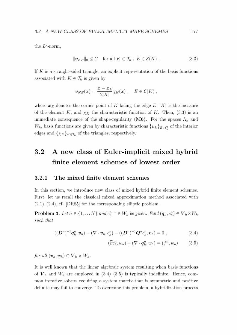
3.2. A NEW CLASS OF EULER-IMPLICIT MHFE SCHEMES 177
the L2-norm,
‖vKE‖0 ≤ C for all K ∈ Th , E ∈ E(K) . (3.3)
If K is a straight-sided triangle, an explicit representation of the basis functions
associated with K ∈ Th is given by
vKE(x) =x− xE
2|K| χK(x) , E ∈ E(K) ,
where xE denotes the corner point of K facing the edge E, |K| is the measure
of the element K, and χK the characteristic function of K. Then, (3.3) is an
immediate consequence of the shape-regularity (M6). For the spaces Λh and
Wh, basis functions are given by characteristic functions µEE∈EIh of the interior
edges and χKK∈Th of the triangles, respectively.
3.2 A new class of Euler-implicit mixed hybrid
finite element schemes of lowest order
3.2.1 The mixed finite element schemes
In this section, we introduce new class of mixed hybrid finite element schemes.
First, let us recall the classical mixed approximation method associated with
(2.1)–(2.4), cf. [DR85] for the corresponding elliptic problem.
Problem 3. Let n ∈ 1, . . . N and cn−1h ∈ Wh be given. Find (qnh, c
nh) ∈ V h×Wh
such that
((Dn)−1qnh,vh)− (∇ · vh, cnh)− ((Dn)−1Qncnh,vh) = 0 , (3.4)
(∂cnh, wh) + (∇ · qnh, wh) = (fn, wh) (3.5)
for all (vh, wh) ∈ V h ×Wh.
It is well known that the linear algebraic system resulting when basis functions
of V h and Wh are employed in (3.4)–(3.5) is typically indefinite. Hence, com-
mon iterative solvers requiring a system matrix that is symmetric and positive
definite may fail to converge. To overcome this problem, a hybridization process

178 CHAPTER 3. MHFE SCHEMES BASED ON THE RT0 ELEMENT
can be employed, where the space V h is replaced by the augmented space V h,
i. e., the continuity of the normal fluxes across interelement boundaries is relaxed,
cf. [BF91]. The continuity constraints are then imposed by requiring additional
equations and introducing Lagrange multipliers from the space Λh. The resulting
hybrid formulation is equivalent to the original formulation. Moreover, by apply-
ing a local elimination procedure, one can derive a linear system in terms of the
Lagrange multipliers only, cf. Sec. 3.2.2. Hence, the resulting system has fewer
unknowns than that of the non-hybrid method. The mixed hybrid formulation
associated with (3.4)–(3.5) reads as follows.
Problem 4. Let n ∈ 1, . . . N and cn−1h ∈ Wh be given. Find (qnh, c
nh, λ
nh) ∈
V h ×Wh × Λh such that
((Dn)−1qnh,vh)−∑K∈Th
(∇ · vh, cnh)K − ((Dn)−1Qncnh,vh)
= −∑K∈Th〈λnh,vh · n∂K〉∂K ,
(3.6)
(∂cnh, wh) +∑K∈Th
(∇ · qnh, wh)K = (fn, wh) , (3.7)
∑K∈Th〈µh, qnh · n∂K〉∂K = 0 (3.8)
for all (vh, wh, µh) ∈ V h ×Wh × Λh.
Here, n∂K denotes the outer unit normal vector of ∂K. The Lagrange multipliers
may be regarded as an approximation of the scalar unknown on the element
interfaces. In fact, they carry some extra information about the exact solution
which can be used to reconstruct a higher order nonconforming approximation in
L2(Ω). We refer to [AB85], where this was shown for an elliptic model problem.
The use of the Lagrange multipliers in the discretization of the advective term is
one of the key ideas in the definition of the new class of methods. Moreover, the
exact velocity field is replaced by the approximation
Qnh := ΠhQ
n =∑K∈Th
∑E∈E(K)
QnKEvKE ∈ V h ,

3.2. A NEW CLASS OF EULER-IMPLICIT MHFE SCHEMES 179
which satisfies (cf. [Dur88])
‖Qn −Qnh‖L∞(Ω) ≤ Ch‖Qn‖W 1,∞(Ω) . (3.9)
Note that in many applications, an approximation of the velocity field Qn is
computed in a preprocessing step by solving Richards’ equation. If the RT0
element is used for this calculation, the coefficients QnKE are directly known.
In the schemes studied here, the advective terms are discretized using the re-
construction operator B : Λh × Wh → V h, which—given a piecewise constant
approximation λnh =∑
E∈EIhλnEµE ∈ Λh of cn on the edges of the triangulation
and the cellwise constant approximation cnh =∑
K∈Th cnKχK—reconstructs an ap-
proximation for the advective flux in the space V h. More precisely, the operator
B is defined to act on Λh ×Wh as
B(λnh, cnh) =
∑K∈Th
∑E∈E(K)
αnKE(cnK , λnE)Qn
KEvKE ,
where the weights αnKE are linear functionals on R×R and satisfy the condition
|αnKE(cnK , λnE)− cnK | ≤ C|λnE − cnK | . (3.10)
In contrast to the standard scheme, where the approximation of the advective
flux relies on the cellwise constant approximations cnK only, the discretization of
the advective fluxes in the mixed methods based on the reconstruction operator Bmay additionally depend on the Lagrange multipliers. Different schemes that are
recovered for specific choices of the weights αnKE are discussed in Section 3.4. The
class of mixed methods based on the reconstruction operator B and the weight
functions αnKE reads as follows.
Problem 5. Let n ∈ 1, . . . N and cn−1h ∈ Wh be given. Find (qnh, c
nh, λ
nh) ∈
V h ×Wh × Λh with the representations
qnh =∑K∈Th
∑E∈E(K)
qnKEvKE , cnh =∑K∈Th
cnKχK , λnh =∑E∈EIh
λnEµE (3.11)

180 CHAPTER 3. MHFE SCHEMES BASED ON THE RT0 ELEMENT
such that
((Dn)−1qnh,vh)−∑K∈Th
(∇ · vh, cnh)K − ((Dn)−1B(λnh, cnh),vh)
= −∑K∈Th〈λnh,vh · n∂K〉∂K ,
(3.12)
(∂cnh, wh) +∑K∈Th
(∇ · qnh, wh)K = (fn, wh) , (3.13)
∑K∈Th〈µh, qnh · n∂K〉∂K = 0 (3.14)
for all (vh, wh, µh) ∈ V h ×Wh × Λh.
Note that an extension of the method to three space dimensions using Raviart–
Thomas elements of lowest order on tetrahedral grids is immediate and requires
only minor changes in the proof of convergence below, cf. Theorem 3.3.4.
For later use, let us finally state the standard upwind-mixed method, cf. [Daw98,
Voh07], which approximates the diffusive flux q = −D∇c.Problem 6. Let n ∈ 1, . . . , N and cn−1
h be given. Find (qnh, cnh) ∈ V h ×Wh
satisfying
((Dn)−1qnh,vh)− (∇ · vh, cnh) = 0 ,
(∂cnh, wh) + (∇ · qnh, wh) +∑K∈Th
∑E∈E(K)
QnKEσ
nKEwK = (fn, wh)
for all (vh, wh) ∈ V h ×Wh, where wK = wh|K and
σnKE =
cnK if QnKE ≥ 0 ,
cnK′ otherwise
if E is a common edge of K and K ′, and
σnKE =
cnK if QnKE ≥ 0 ,
0 otherwise
if E is a boundary edge.

3.2. A NEW CLASS OF EULER-IMPLICIT MHFE SCHEMES 181
3.2.2 Static condensation
Let us assume for a moment that there exists a unique solution (qnh, cnh, λ
nh) ∈ V h×
Wh × Λh of Problem 5 having the basis representations (3.11). Employing these
representations in the equations for the fluxes (3.12), using the basis functions as
test functions in (3.12)–(3.14) and the relations
(∇ · vKE, χK)K = 1 , 〈µE,vKE′ · n∂K〉∂K = δEE′ for K ∈ Th , E,E ′ ∈ E(K) ,
the following system of linear equations for the fluxes is obtained from (3.12):∑E∈E(K)
qnKE((Dn)−1vKE,vKE′)−∑
E∈E(K)
QnKEα
nKE(cnK , λ
nE)((Dn)−1vKE,vKE′)
= cnK − λE′ for all K ∈ Th , E ′ ∈ E(K) .
DefiningBnKE′E := ((Dn)−1vKE,vKE′),B
nK := Bn
KEE′E,E′∈E(K),C := (1, 1, 1)T ,
qnK = qnKEE∈E(K), λnK = λnEE∈E(K), these equations can be rewritten in matrix
form as
BnKq
nK = CcnK +Bn
K
QnKE1
αnKE1(cnK , λ
nE1
)
QnKE2
αnKE2(cnK , λ
nE2
)
QnKE3
αnKE3(cnK , λ
nE3
)
− λnK , K ∈ Th . (3.15)
It is easy to show that the matricesBnK are positive definite. Hence, the equations
(3.15) can be solved explicitly for the flux unknowns on each element K ∈ Th. In
the next step, the fluxes are inserted into the mass conservation equations (3.13)
to obtain a representation cnK = cnK(λnK) of the scalar unknown in terms of the
Lagrange multipliers. Finally, by substituting the flux and scalar unknowns into
the equations (3.14), a linear system for the Lagrange multipliers remains to be
solved in each time step. Once it has been solved, the other variables can be
reconstructed efficiently on each element in a postprocessing step. Note that this
static condensation process can be applied only if the upwind weights depend on
variables defined on a single element K.

182 CHAPTER 3. MHFE SCHEMES BASED ON THE RT0 ELEMENT
3.3 Error analysis of the fully discrete problem
In this section, we present the error analysis of the mixed hybrid finite element
scheme defined in Problem 5. First, let us demonstrate existence and uniqueness
for the scheme (3.12)–(3.14).
Theorem 3.3.1. Assume (A1)-(A2). Then, for every n ∈ 1, . . . , N, Prob-
lem 5 admits a unique solution.
Proof. Since the problem is linear, it suffices to show uniqueness. Thus, let
cn−1h be given, and assume that there exist two solutions (qnh,1, c
nh,1, λ
nh,1) and
(qnh,2, cnh,2, λ
nh,2) ∈ V h × Wh × Λh of (3.12)–(3.14), where cnh,i and λnh,i have the
basis representations
cnh,i =∑K∈Th
cnK,iχK , λnh,i =∑E∈EIh
λnE,iµE , i = 1, 2 ,
respectively. Then, by subtracting, the error equations
((Dn)−1(qnh,1 − qnh,2),vh)−∑K∈Th
(∇ · vh, cnh,1−cnh,2)K +∑K∈Th〈λnh,1−λnh,2,vh · n∂K〉∂K
−∑K∈Th
∑E∈E(K)
QnKEα
nKE(cnK,1 − cnK,2, λnE,1 − λnE,2)((Dn)−1vKE,vh) = 0 ,
(3.16)
(cnh,1 − cnh,2, wh) + τ∑K∈Th
(∇ · (qnh,1 − qnh,2), wh)K = 0 , (3.17)
∑K∈Th〈µh, (qnh,1 − qnh,2) · n∂K〉∂K = 0 (3.18)
hold for all (vh, wh, µh) ∈ V h×Wh×Λh. Next, we proceed similarly as in [AB85]
to obtain an estimate for the errors ‖λnh,1 − λnh,2‖0,E on the edges. For K ∈ Thand E ∈ E(K) let τE denote the unique element of V h with supp(τE) ⊆ K and
τE · nE′ =
λnh,1 − λnh,2 if E = E ′ ,
0 otherwise

3.3. ERROR ANALYSIS OF THE FULLY DISCRETE PROBLEM 183
for all edges E ′ ∈ E(K). Then, it follows from a simple scaling argument that
hK‖τE‖1,K + ‖τE‖0,K ≤ Ch1/2K ‖λnh,1 − λnh,2‖0,E , (3.19)
and we obtain
‖λnh,1 − λnh,2‖0,E ≤ C(h
1/2K ‖qnh,1 − qnh,2‖0,K + h
−1/2K ‖cnh,1 − cnh,2‖0,K
+ h1/2K
∑E′∈E(K)
|E ′|(|cnK,1 − cnK,2|+ |λnE′,1 − λnE′,2|))
≤ C(h
1/2K ‖qnh,1 − qnh,2‖0,K + h
−1/2K ‖cnh,1 − cnh,2‖0,K
+ hK∑
E′∈E(K)
‖λnh,1 − λnh,2‖0,E′)
by using τE as a test function in (3.16) and employing (3.26) and (3.19), respec-
tively. Summing this estimate over the edges E ∈ E(K) and pushing back the
last term for h sufficiently small yields
‖λnh,1 − λnh,2‖0,E ≤ C(h
1/2K ‖qnh,1 − qnh,2‖0,K + h
−1/2K ‖cnh,1 − cnh,2‖0,K
). (3.20)
Next, we take vh := τ(qnh,1 − qnh,2), wh := cnh,1 − cnh,2 and µh := τ(λnh,1 − λnh,2) as
test functions in (3.16)–(3.18) and add the resulting equations to find
τ((Dn)−1(qnh,1 − qnh,2), qnh,1 − qnh,2) + ‖cnh,1 − cnh,2‖20
− τ∑K∈Th
∑E∈E(K)
QnKEα
nKE(cnK,1 − cnK,2, λnE,1 − λnE,2)((Dn)−1vKE, q
nh,1 − qnh,2) = 0 .
Further, using (3.20), (3.3), and (A1)-(A2), we obtain
‖cnh,1 − cnh,2‖20 + τ‖qnh,1 − qnh,2‖2
0 ≤ Cτ∑K∈Th
∑E∈E(K)
|E||λnE,1 − λnE,2|‖qnh,1 − qnh,2‖0,K
+ Cτ∑K∈Th
∑E∈E(K)
|E||cnK,1 − cnK,2|‖qnh,1 − qnh,2‖0,K

184 CHAPTER 3. MHFE SCHEMES BASED ON THE RT0 ELEMENT
≤ Cτ∑K∈Th
h1/2K
∑E∈E(K)
‖λnh,1 − λnh,2‖0,E‖qnh,1 − qnh,2‖0,K
+ Cτ∑K∈Th
‖cnh,1 − cnh,2‖0,K‖qnh,1 − qnh,2‖0,K
≤ Cτ∑K∈Th
hK‖qnh,1 − qnh,2‖20,K + Cτ
∑K∈Th
‖cnh,1 − cnh,2‖0,K‖qnh,1 − qnh,2‖0,K
≤ Cδ‖cnh,1 − cnh,2‖20 +
Cτ 2
4δ‖qnh,1 − qnh,2‖2
0 + Cτh‖qnh,1 − qnh,2‖20
so that, by taking δ, τ and h sufficiently small, cnh,1 − cnh,2 and qnh,1 − qnh,2 vanish.
From (3.20), we infer that λnh,1 − λnh,2 vanishes.
Let us now turn to the error analysis of the fully discrete mixed hybrid scheme
(3.12)–(3.14). One of the main steps in the proof of convergence is the derivation
of a priori estimates for the differences |λnE−cnK | which occur in the error equations
resulting from (2.5)–(2.6) and (3.12)–(3.14). This is done in the following lemma
by employing similar techniques as in the a posteriori error analysis in [AB85],
where the Lagrange multipliers were used to obtain a higher order approximation
of the scalar unknown by postprocessing.
Lemma 3.3.2. Let (A1)-(A3) hold and assume that the solution (q, c) of Prob-
lem 2 satisfies (A4). Further, let (qnh, cnh, λ
nh) ∈ V h ×Wh × Λh be the solution
of Problem 5. Then, for h sufficiently small, there exists a constant C > 0,
independent of n and h, such that∑K∈Th
∑E∈E(K)
|E|2(λnE − cnK)2 ≤ C(‖cn − cnh‖2
0 + h2‖qn − qnh‖20
+ h2‖Qnhcnh −Qncn‖2
0 + h2‖cn‖21
).
(3.21)
Proof. In the first step, we show that
‖λnh −Q0hcn‖0,E ≤C
(h
1/2K ‖qn − qnh‖0,K + h
1/2K
∑E′∈E(K)
|E ′||λnE′ − cnK |
+ h1/2K ‖Qn
hcnh −Qncn‖0,K + h
−1/2K ‖cn − cnh‖0,K
),
(3.22)
where Q0h denotes the projection operator defined locally by L2(E)-orthogonal

3.3. ERROR ANALYSIS OF THE FULLY DISCRETE PROBLEM 185
projection onto P0(E) for some E ∈ Eh, i. e.,
〈Q0hcn − cn, 1〉E = 0 for all E ∈ Eh .
For some fixed K ∈ Th and E ∈ E(K), define τE as the unique element of V h
such that supp(τE) ⊆ K and
τE · nE′ =
λnh −Q0hcn if E = E ′,
0 otherwise
for all E ′ ∈ E(K). A simple scaling argument shows that
hK‖τE‖1,K + ‖τE‖0,K ≤ Ch1/2K ‖λnh −Q0
hcn‖0,E . (3.23)
Next, we use τE as a test function in (3.12) to obtain
((Dn)−1qnh, τE)K − (∇ · τE, cnh)K −∑
E′∈E(K)
QnKE′α
nKE′((D
n)−1vKE′ , τE)K
= −〈λnh, λnh −Q0hcn〉E .
(3.24)
Moreover, (2.7) and Green’s formula imply
((Dn)−1qn, τE)K − (∇ · τE, cn)K − ((Dn)−1Qncn, τE)K = −〈cn, λnh −Q0hcn〉E .
(3.25)
Subtracting (3.24) from (3.25), using the definition of Q0h, the estimate
|QnKE| = |〈Qn · nE, 1〉E| ≤ C|E| , (3.26)

186 CHAPTER 3. MHFE SCHEMES BASED ON THE RT0 ELEMENT
the property (3.3), the condition (3.10), and the assumption (A1), we get
‖λnh −Q0hcn‖2
0,E = 〈λnh −Q0hcn, λnh − cn〉E
= ((Dn)−1(qn − qnh), τE)K − (∇ · τE, cn − cnh)K
−∑
E′∈E(K)
QnKE′(c
nK − αnKE′)((Dn)−1vKE′ , τE)K + ((Dn)−1(Qn
hcnh −Qncn), τE)K
≤ C(‖qn − qnh‖0,K‖τE‖0,K + ‖cn − cnh‖0,K‖τE‖1,K
+∑
E′∈E(K)
|E ′||λnE′ − cnK |‖τE‖0,K + ‖Qnhcnh −Qncn‖0,K‖τE‖0,K
).
Then, (3.22) follows from combining the last estimate with (3.23). Next, we use
the Lagrange multipliers to define a nonconforming approximation cnh of cn in the
space PCR1 (Th) of linear Crouzeix-Raviart elements by means of
Q0hcnh = λnh . (3.27)
Note that cnh is uniquely determined according to [AB85, Lemma 2.1], see also the
remark on boundary elements having a curved edge after Lemma 4.2 in [BDM85].
Similarly, we define cnh ∈ PCR1 (Th) to be the nonconforming projection of cn by
means of
Q0h(c
n − cnh) = 0 . (3.28)
Then, by standard arguments, it follows that
‖cnh − cn‖0 ≤ Ch‖cn‖1 . (3.29)
Moreover, from (3.27) and (3.28), we have
Q0h(c
nh − cnh) = λnE −Q0
hcn ,
which implies
‖cnh − cnh‖0,K ≤ Ch1/2K
∑E∈E(K)
‖λnh −Q0hcn‖0,E

3.3. ERROR ANALYSIS OF THE FULLY DISCRETE PROBLEM 187
by [AB85, Lemma 2.1]. Combining this with (3.22), we obtain
‖cnh − cnh‖0,K ≤ C(hK‖qn − qnh‖0,K + ‖cn − cnh‖0,K + hK‖Qn
hcnh −Qncn‖0,K
+ hK∑
E∈E(K)
|E||λnE − cnK |)
so that, by summing over all elements,
‖cnh − cnh‖20 ≤ C
(h2‖qn − qnh‖2
0 + ‖cn − cnh‖20 + h2‖Qn
hcnh −Qncn‖2
0
+ h2∑K∈Th
∑E∈E(K)
|E|2(λnE − cnK)2).
(3.30)
Hence, from (3.29) and (3.30), we get
‖cnh − cnh‖20 ≤ 3‖cnh − cnh‖2 + 3‖cnh − cn‖2
0 + 3‖cn − cnh‖20
≤ C(h2‖qn − qnh‖2
0 + ‖cn − cnh‖20 + h2‖Qn
hcnh −Qncn‖2
0
+ h2∑K∈Th
∑E∈E(K)
|E|2(λnE − cnK)2 + h2‖cn‖21
).
(3.31)
Now, we use that for any piecewise linear polynomial ph ∈⊕
K∈Th P1(K), the
estimate
‖ph‖L1(∂K) ≤ C‖ph‖0,K
holds, cf. [BF91, p. 112]. Then, for any K ∈ Th and E ∈ E(K),
|E|(λnE − cnK) = 〈cnh − cnh, 1〉E ≤ C‖cnh − cnh‖L1(∂K) ≤ C‖cnh − cnh‖0,K .
Finally, combining the last estimate with (3.31) yields∑K∈Th
∑E∈E(K)
|E|2(λnE − cnK)2 ≤ C‖cnh − cnh‖20 ≤ C
(h2‖qn − qnh‖2
0 + ‖cn − cnh‖20
+ h2‖Qnhcnh −Qncn‖2
0 + h2∑K∈Th
∑E∈E(K)
|E|2(λnE − cnK)2 + h2‖cn‖21
),
and (3.21) follows by pushing back the last term on the right hand side for
sufficiently small h.

188 CHAPTER 3. MHFE SCHEMES BASED ON THE RT0 ELEMENT
For later use, we state the following discrete integration by parts formula.
Lemma 3.3.3. Let (an)n∈N0 and (bn)n∈N0 be real sequences and let m ∈ N. Then,
it holds that
m∑n=1
(an − an−1)bn = ambm − a0b0 −m∑n=1
an−1(bn − bn−1) .
Theorem 3.3.4. Let the assumptions (A1)–(A3) hold and denote by (q, c) ∈L2(J ;H(div,Ω))×H1(J ;L2(Ω)) the unique solution of Problem 2. Moreover, let
τ and h be sufficiently small such that for every n ∈ 1, . . . , N there exists a
unique solution (qnh, cnh, λ
nh) ∈ V h × Wh × Λh of Problem 5. Then, if (A4) is
satisfied and c0h = Phc0, there exists a constant C > 0, independent of τ and h,
such that
maxm∈1,...,N
‖c(·, tm)− cmh ‖20 + τ
N∑n=1
‖q(·, tn)− qnh‖20 ≤ C(τ 2 + h2) . (3.32)
Proof. We take t = tn in (2.5)–(2.6), subtract (3.12)–(3.13) from the resulting
equations and use the properties (3.1a)–(3.1b) to obtain the error equations
((Dn)−1(qn − qnh),vh)−∑K∈Th
(∇ · vh, Phcn − cnh)K − ((Dn)−1Qncn,vh)
+∑K∈Th
∑E∈E(K)
QnKEα
nKE((Dn)−1vKE,vh) =
∑K∈Th〈λnh,vh · n∂K〉∂K ,
(3.33)
(∂tcn − ∂cnh, wh) +
∑K∈Th
(∇ · (Πhqn − qnh), wh)K = 0 , (3.34)
∑K∈Th〈(Πhq
n − qnh) · n∂K , µh〉∂K = 0 (3.35)
for all (vh, wh, µh) ∈ V h × Wh × Λh. Note that our regularity assumptions
allow the evaluation of c and q and all coefficient functions at t = tn. Taking
vh := Πhqn−qnh, wh := Phc
n−cnh and µh := −λnh as test functions in (3.33)–(3.35)

3.3. ERROR ANALYSIS OF THE FULLY DISCRETE PROBLEM 189
and adding the resulting equations yields
((Dn)−1(qn − qnh),Πhqn − qnh)− ((Dn)−1Qncn,Πhq
n − qnh)
+ (∂tcn − ∂cnh, Phcn − cnh) +
∑K∈Th
∑E∈E(K)
QnKEα
nKE((Dn)−1vKE,Πhq
n − qnh) = 0 .
The last identity can be rewritten equivalently as
((Dn)−1(qn − qnh),Πhqn − qnh) + ((Dn)−1(Qn
hcnh −Qncn),Πhq
n − qnh)
+∑K∈Th
∑E∈E(K)
QnKE(αnKE − cnK)((Dn)−1vKE,Πhq
n − qnh)
+ (∂tcn − ∂cnh, Phcn − cnh) = 0 .
(3.36)
Further, for any m ∈ N with 1 ≤ m ≤ N , by summing (3.36) from n = 1, . . . ,m,
multiplying by 2τ and expanding, we obtain
T1 + . . .+ T8 := 2τm∑n=1
((Dn)−1(qn − qnh), qn − qnh)
+ 2τm∑n=1
((Dn)−1(qn − qnh),Πhqn − qn)
+ 2τm∑n=1
((Dn)−1(Qnhcnh −Qncn),Πhq
n − qnh)
+ 2τm∑n=1
(∂tcn − ∂cn, cn − cnh)
+ 2τm∑n=1
(∂tcn − ∂cn, Phcn − cn)
+ 2τm∑n=1
(∂(cn − cnh), cn − cnh)
+ 2τm∑n=1
(∂(cn − cnh), Phcn − cn)
+ 2τm∑n=1
∑K∈Th
∑E∈E(K)
QnKE(αnKE − cnK)((Dn)−1vKE,Πhq
n − qnh)
= 0 .

190 CHAPTER 3. MHFE SCHEMES BASED ON THE RT0 ELEMENT
We now proceed to estimate separately each of the terms T1, . . . T8. First, the
terms T1 and T6 are bounded from below. Note that sinceD is uniformly positive
definite, D−1 is also uniformly positive definite. Thus, we have
T1 = 2τm∑n=1
((Dn)−1(qn − qnh), qn − qnh) ≥ Cτm∑n=1
‖qn − qnh‖20 . (3.37)
By the identity 2a(a− b) = a2 − b2 + (a− b)2, we find
T6 = 2m∑n=1
((cn − cnh)− (cn−1 − cn−1h ), cn − cnh)
=m∑n=1
‖cn − cnh‖20 −
m∑n=1
‖cn−1 − cn−1h ‖2
0 +m∑n=1
‖cn − cnh − cn−1 + cn−1h ‖2
0
≥ ‖cm − cmh ‖20 − ‖c0 − c0
h‖20 .
(3.38)
All other terms are passed to the right hand side and bounded from above. Using
a weighted Young’s inequality, we get for any δ2 > 0
|T2| ≤ Cδ2τm∑n=1
‖qn − qnh‖20 +
Cτ
δ2
m∑n=1
‖Πhqn − qn‖2
0 . (3.39)
The term T3 is rewritten as
T3 = 2τm∑n=1
((Dn)−1(Qnhcnh −Qncn), qn − qnh)
+ 2τm∑n=1
((Dn)−1(Qnhcnh −Qncn,Πhq
n − qn) =: T31 + T32 .
Then, for h sufficiently small, it follows from (3.9) and the regularity of Q that
‖Qnhcnh −Qncn‖0 ≤ ‖Qn
h(cn − cnh)‖0 + ‖(Qn −Qnh)cn‖0
≤ ‖Qnh‖L∞(Ω)‖cn − cnh‖0 + ‖Qn −Qn
h‖L∞(Ω)‖cn‖0
≤ C(‖cn − cnh‖0 + h‖cn‖0) .
(3.40)
Moreover, from the uniform boundedness of D−1 and a weighted Young’s in-

3.3. ERROR ANALYSIS OF THE FULLY DISCRETE PROBLEM 191
equality, we obtain that for any δ3 > 0
|T31| ≤Cτ
δ3
m∑n=1
‖Qnhcnh −Qncn‖2
0 + Cδ3τm∑n=1
‖qn − qnh‖20
≤ Cτ
δ3
m∑n=1
‖cn − cnh‖20 +
Ch2τ
δ3
m∑n=1
‖cn‖20 + Cδ3τ
m∑n=1
‖qn − qnh‖20 .
(3.41)
Similarly, we derive the estimate
|T32| ≤ Cτ
m∑n=1
‖cn − cnh‖20 + Ch2τ
m∑n=1
‖cn‖20 + Cτ
m∑n=1
‖Πhqn − qn‖2
0 . (3.42)
Next, we use Bochner’s inequality, the Cauchy-Schwarz inequality and the regu-
larity of c to find
|T4| ≤1
τ
m∑n=1
‖τ∂tcn − cn + cn−1‖20 + τ
m∑n=1
‖cn − cnh‖20
=1
τ
m∑n=1
∥∥∥∥∫ tn
tn−1
∫ tn
s
∂ttc(η) dη ds
∥∥∥∥2
0
+ τm∑n=1
‖cn − cnh‖20
≤ τ 2
m∑n=1
∫ tn
tn−1
‖∂ttc(η)‖20 dη + τ
m∑n=1
‖cn − cnh‖20
≤ τ 2‖∂ttc‖2L2(J ;L2(Ω)) + τ
m∑n=1
‖cn − cnh‖20
≤ Cτ 2 + τm∑n=1
‖cn − cnh‖20 .
(3.43)
Analogously,
|T5| ≤ τ 2‖∂ttc‖2L2(J ;L2(Ω)) + τ
m∑n=1
‖Phcn − cn‖20
≤ Cτ 2 + τ
m∑n=1
‖Phcn − cn‖20 .
(3.44)

192 CHAPTER 3. MHFE SCHEMES BASED ON THE RT0 ELEMENT
For T7, we employ Lemma 3.3.3 and the definition c0h = Phc0 to get
|T7| ≤ δ7‖cm − cmh ‖20 +
1
δ7
‖Phcm − cm‖20 + (2 + τ)‖Phc0 − c0‖2
0
+ τ
m−1∑n=1
‖cn − cnh‖20 +
1
τ
m∑n=1
‖(Ph − I)(cn − cn−1)‖20 ,
(3.45)
where I denotes the identity operator. Denoting the last term on the right hand
side of (3.45) by T71, we obtain from Bochner’s inequality, the Cauchy-Schwarz
inequality and the regularity of c that
T71 ≤Ch2
τ
m∑n=1
‖cn − cn−1‖21 =
Ch2
τ
m∑n=1
∥∥∥∥∫ tn
tn−1
∂tc(η) dη
∥∥∥∥2
1
≤ Ch2
∫ tm
0
‖∂tc(η)‖21 dη ≤ Ch2‖∂tc‖2
L2(J ;H1(Ω))
≤ Ch2 .
Consequently,
|T7| ≤ δ7‖cm − cmh ‖20 +
1
δ7
‖Phcm − cm‖20 + (2 + τ)‖Phc0 − c0‖2
0
+ τm∑n=1
‖cn − cnh‖20 + Ch2 .
(3.46)
For the remaining term T8, we combine (3.26) and (3.3) to find
|T8| ≤Cτ
δ8
m∑n=1
∑K∈Th
∑E∈E(K)
|E|2(λnE − cnK)2 + Cδ8τm∑n=1
‖Πhqn − qn‖2
0
+ Cδ8τm∑n=1
‖qn − qnh‖20 ,

3.4. CHOICE OF THE WEIGHT FUNCTION 193
and it follows from Lemma 3.3.2 and (3.40) that
|T8| ≤C
δ8
(h2τ
m∑n=1
‖cn‖21 + τ
m∑n=1
‖cn − cnh‖20 + h2τ
m∑n=1
‖qn − qnh‖20
+ h2τ
m∑n=1
‖cn − cnh‖20 + h4τ
m∑n=1
‖cn‖20
)+ Cτδ8
m∑n=1
‖Πhqn − qn‖2
0
+ Cτδ8
m∑n=1
‖qn − qnh‖20 .
(3.47)
Finally, by collecting the estimates (3.37)–(3.47), choosing δ2, δ3, δ7, δ8, τ and h
sufficiently small, and pushing back terms to the left hand side, we obtain
‖cm − cmh ‖20 + τ
m∑n=1
‖qn − qnh‖20 ≤ Cτ 2 + Ch2 + Cτ
m∑n=1
‖Πhqn − qn‖2
0
+ Cτm∑n=1
‖Phcn − cn‖20 + C‖Phc0 − c0‖2
0 + C‖Phcm − cm‖20
+ Ch2τm∑n=1
‖cn‖20 + Cτ
m∑n=1
‖cn − cnh‖20 + Ch2τ
m∑n=1
‖cn‖21 ,
and (3.32) follows from the properties of the projectors, the regularity of q and
c, and by applying the discrete Gronwall lemma.
Note that since we applied the discrete Gronwall lemma, the constant in the error
estimate (3.32) is potentially large. This is in accordance with the convergence
analysis of the upwind-mixed methods in [Daw91] and [Daw93]. In [DA99], the
use of the Gronwall lemma was avoided, but only suboptimal convergence was
obtained for the semidiscrete problem.
3.4 Choice of the weight function
The proof of convergence given in the previous section applies to all schemes that
are obtained if the weight functions αnKE satisfy (3.10). This condition holds for

194 CHAPTER 3. MHFE SCHEMES BASED ON THE RT0 ELEMENT
the upwind-mixed method resulting from the choice
αn,upKE (cnK , λ
nE) =
cnK if QnKE ≥ 0 ,
2λnE − cnK otherwise ,
which was studied numerically in the paper [RSH+11] in the context of reactive
transport simulation. This upwind weighting formula is motivated by the fact
that the Lagrange multipliers represent an approximation of the scalar unknown
on the edges. Hence, the expression 2λnE − cnK may be regarded as an extrapo-
lation of the concentration on the adjacent cell. The advantage of the resulting
upwind-mixed hybrid method is that it is fully local, i. e., it does not incorporate
information of adjacent cells. Consequently, static condensation can be employed
to eliminate the flux and the scalar unknowns from the system, cf. Section 3.2.2.
This implies that the method can be implemented more efficiently than the stan-
dard upwind-mixed method stated in Problem 6, where the definition of the
upwind weights explicitly involves concentration values of adjacent grid cells. In
the next section, the upwind-mixed hybrid method resulting from the choice αn,upKE
is compared with the standard upwind-mixed scheme in terms of accuracy and
efficiency.
It is well-known that full upwind methods may introduce a significant amount of
numerical diffusion, which leads to an artificial smearing of the numerical solution.
We refer to the numerical experiments in [RSH+11], where the amount of artificial
diffusion of the upwind-mixed hybrid method was quantified and compared with
other discretization schemes. One possibility to reduce the amount of artificial
diffusion is to use the partial upwind scheme obtained for the choice
αn,partKE (cnK , λ
nE) =
cnK if QnKE ≥ 0 ,
(1− νE)cnK + νE(2λnE − cnK) otherwise ,
which obviously satisfies condition (3.10). Here, νE ∈ [0, 1] denotes a coefficient
describing the amount of upstream weighting. It may depend on the local grid
Peclet number to ensure that upwinding is only employed in those parts of the
domain where the flow is advection–dominant. Obviously, for νE = 1, the full
upwind scheme is recovered.

3.4. CHOICE OF THE WEIGHT FUNCTION 195
Qn
cnK1b cnK2
bλnEb
E
Figure 3.1: Scalar unknowns and Lagrange multiplier associated with the com-mon edge of two adjacent triangles K1 and K2
Further admissible choices for the weight function are given by
αn,lagKE (cnK , λ
nE) = λnE ,
which was tested in [RSH+11] and proved to be robust for moderately advection–
dominant problems, and
αn,stdKE (cnK , λnE) = cnK ,
which represents the standard scheme (3.6)–(3.8) with the only difference that
Qn was approximated by Qnh. Another full upwind scheme is recovered for the
choice
αn,up,2KE (cnK , λ
nE) =
cnK if QnKE ≥ 0 ,
λnE otherwise .
This scheme was tested numerically in the paper [BFK14] and performed favor-
ably compared to an upwind-weighted finite volume scheme in terms of robust-
ness, monotonicity properties, and the amount of artificial numerical diffusion
introduced by both methods.

196 CHAPTER 3. MHFE SCHEMES BASED ON THE RT0 ELEMENT
3.5 Numerical results
In this section, we present a numerical example for the upwind-mixed hybrid
method obtained for the weight αn,upKE defined in the previous section. More
precisely, we provide computational evidence that our error estimates are sharp,
and we compare the upwind-mixed hybrid method with the standard upwind-
mixed method of Dawson [Daw98]. Further numerical examples from the context
of contaminant biodegradation with advection–dominated flow are included in
[Bru10]. Moreover, in [RSH+11], the numerical diffusion of the upwind-mixed
hybrid method was quantified and compared with other discretization methods.
In our computations, we solve problem (1.1)–(1.3) on the unit square Ω = (0, 1)2
and the time interval J = (0, 1). The (scalar) diffusion coefficient and the velocity
field are given by D = 1 and Q = (0,−1)T , respectively. The source term f is
chosen so that c(x, y, t) = x(1− x)y(1− y)e−t represents the analytical solution
of the problem, and c0 := c(·, 0) is imposed as the initial value. A simple uniform
triangular mesh with h =√
2 is used as a coarse grid, and τ = 0.5 is chosen as
the initial time step size. In each level of refinement, h and τ are halved, and the
errors
Eτ,h =
‖c(·, tN)− cNh ‖2
0 + τN∑n=1
‖q(·, tn)− qnh‖20
1/2
are computed. For the upwind scheme of Dawson, we use qnh = qnh + Qcnh ∈RT0(Ω, Th) as an approximation of the total flux, where qh denotes the flux vari-
able of the scheme, which approximates the diffusive flux q = −D∇c. Both
methods were implemented in the software package M++ [Wie, Wie05]. To han-
dle the saddle point problems arising from the standard upwind-mixed scheme,
the linear systems are solved with a direct solver based on the SuperLU library
[Li05]. The results of the computations are summarized in Tables 3.1 and 3.2.
They clearly show optimal first order convergence in h and τ for our upwind-
mixed hybrid scheme. Hence, the error bound of Theorem 3.3.4 is sharp. More-
over, the magnitude of the errors almost coincides for both methods, while the
computation time was 50% lower on the finest mesh for the hybrid scheme.
On the one hand, this is due to a lower number of global unknowns resulting
from hybridization and employing static condensation, cf. Sec. 3.2.2. On the

3.5. NUMERICAL RESULTS 197
Ref. level # unknowns Eτ,h reduction CPU time [s]
1 16 3.685e-2 0.01
2 56 2.297e-2 1.60 0.03
3 208 1.236e-2 1.85 0.09
4 800 6.345e-3 1.95 0.47
5 3136 3.205e-3 1.98 3.88
6 12416 1.610e-3 1.99 33.11
7 49408 8.067e-4 2.00 305.90
Table 3.1: Numerical results for the upwind-mixed hybrid method
Ref. level # unknowns Eτ,h reduction CPU time [s]
1 24 3.507e-2 0.01
2 88 2.264e-2 1.54 0.03
3 226 1.234e-2 1.83 0.10
4 1312 6.349e-3 1.94 0.66
5 5184 3.208e-3 1.98 5.79
6 20608 1.611e-3 1.99 57.52
7 82176 8.068e-4 2.00 709.00
Table 3.2: Numerical results for the upwind-mixed method [Daw98]
other hand, the linear system associated with our method is sparser than that
corresponding to the non-hybrid method. Hence, the linear solver is faster and
less memory is required during the computation.

Chapter 4
Mixed hybrid finite element
discretizations based on the
BDM1 element
In the previous chapter, a new class of mixed hybrid finite element methods
based on the RT0 element was studied, where the advective fluxes are discretized
using the Lagrange multipliers introduced during hybridization. Depending on
the particular choice of the weight functions, different schemes are recovered from
this general class, e. g., the standard scheme or an upwind-mixed hybrid scheme
designed for strongly advection–dominated problems.
In this chapter, similar ideas are applied to approximations based on the BDM1
element. More precisely, we will show that suboptimal convergence for the flux
variable, which is known to arise when the standard BDM1 scheme is employed to
advection–diffusion problems, can be overcome by using the Lagrange multipliers
for the discretization of the advective fluxes. This observation was made and
confirmed numerically in the paper [BRBK12]. The error analysis is provided in
the article [BFK15].
198

4.1. SUBOPTIMAL CONVERGENCE OF THE STANDARD SCHEME 199
4.1 Suboptimal convergence of the standard non-
hybrid scheme
Using the Raviart–Thomas spaces for the discretization of (1.1)–(1.3), the flux
and the scalar unknown are approximated with the same order of convergence.
For applications where the main interest lies in the flux variable, the BDM
spaces were introduced [BDM85], which are able to approximate the flux to one
order higher than the scalar variable. Indeed, if the BDM1 mixed finite element
method is used to discretize a pure second order elliptic diffusion equation, the
flux is approximated with second order accuracy in the L2 norm. Error estimates
in L2(Ω) and L∞(Ω) for general second order elliptic problems with nonvanish-
ing advection using the BDM family of methods were derived in [Dem02] and
[Dem04], respectively. More precisely, it was shown that the total flux variable
consisting of diffusive and advective transport is approximated with first order
accuracy in L2(Ω), which is suboptimal since the same order of convergence is
obtained by the computationally less expensive RT0 element. This phenomenon
of suboptimal convergence may occur whenever the mixed finite element spaces
employed use polynomials of higher order for the approximation of the flux vari-
able than for the approximation of the scalar variable. The order of convergence
is then limited by the first order accuracy of the approximation for the conserved
quantity itself.
In the following, we will present a modified mixed hybrid BDM1 scheme which
restores optimal second order convergence of the flux variable in the presence of
an advective transport term. The modification consists in replacing the cellwise
constant approximation of the scalar unknown in the definition of the discrete
advective flux by a reconstruction based on the interelement Lagrange multipliers.
This is motivated by the well-known fact that the Lagrange multipliers carry some
higher order information about the scalar unknown.

200 CHAPTER 4. MHFE SCHEMES BASED ON THE BDM1 ELEMENT
b
b b
b
b b
K
Figure 4.1: Degrees of freedom of the local BDM1 space
4.2 The modified hybrid scheme
Mixed approximation spaces and projections
In the following, we assume that the domain Ω ⊂ R2 is polygonally bounded
and that Thh>0 denotes a family of shape-regular triangulations of Ω where
all triangles have straight edges only, cf. (M1)–(M3), (M5)–(M6). For the
discretization with the BDM1 mixed finite element method, let
V h = BDM1(Ω, Th) = v ∈ H(div,Ω) : v|K ∈ BDM1(K) for all K ∈ Th ,
Wh = w ∈ L2(Ω) : w|K ∈ P0(K) for all K ∈ Th ,
where BDM1(K) = (P1(K))2. The degrees of freedom for BDM1(K) are illus-
trated in Figure 4.1.
The standard BDM1 mixed finite element method for approximating the total
flux q = −D∇c+Qc reads as follows, cf. [Dem02].
Problem 7. Let n ∈ 1, . . . N and cn−1h ∈ Wh be given. Find (qnh, c
nh) ∈ V h×Wh
such that
((Dn)−1qnh,vh)− (∇ · vh, cnh)− ((Dn)−1Qncnh,vh) = 0 , (4.1)
(∂cnh, wh) + (∇ · qnh, wh) = (fn, wh) (4.2)
for all (vh, wh) ∈ V h ×Wh.
In the following, we want to consider the hybrid problem formulation associated
with (4.1)–(4.2). For the BDM1 element, the Lagrange multipliers are linear
functions on each edge and may be discontinuous at the vertices. The approxi-

4.2. THE MODIFIED HYBRID SCHEME 201
mation spaces associated with the hybrid formulation are defined as
V h = v ∈ (L2(Ω))2 : v|K ∈ BDM1(K) for all K ∈ Th ,
Λh = λ ∈ L2(Eh) : λ|E ∈ P1(E) for all E ∈ EIh , λ|E = 0 for all E ∈ EDh .
The hybrid formulation associated with (4.1)–(4.2) reads as follows.
Problem 8. Let n ∈ 1, . . . N and cn−1h ∈ Wh be given. Find (qnh, c
nh, λ
nh) ∈
V h ×Wh × Λh such that
((Dn)−1qnh,vh)−∑K∈Th
(∇ · vh, cnh)K((Dn)−1Qncnh,vh)
= −∑K∈Th〈λnh,vh · n〉∂K , (4.3)
(∂cnh, wh) +∑K∈Th
(∇ · qnh, wh)K = (fn, wh) , (4.4)
∑K∈Th〈µh, qnh · n〉∂K = 0 (4.5)
for all (vh, wh, µh) ∈ V h ×Wh × Λh.
To obtain an algebraic formulation of the scheme (4.3)–(4.5), basis functions of
the involved function spaces must be specified. The space Λh consists of functions
which are defined on the edges of the triangulation and which are linear on each
edge. A basis of this space is given by functions vanishing everywhere except for
one interior edge and taking the value 0 at one endpoint and the value 1 at the
other endpoint of this edge. More precisely, for an interior edge E ∈ EIh with
vertices x1E and x2
E, we denote by µiE the function in Λh which takes the value 1
in xiE and the value 0 at the other endpoint of E and vanishes on all other edges.
For V h we define the basis functions to be the vector fields that vanish on every
triangle except for one triangle K, on which the normal flux is prescribed to be
zero at every edge except for one edge E ∈ E(K); on this edge, we require the
(outward) normal flux to be 2/|F | at the point 13(2x1
E + x2E) and to be 0 at the
point 13(x1
E + 2x2E). These basis functions are obtained by transforming the basis
functions on the unit reference triangle K (cf. Table 4.1) to an arbitrary triangle
K ∈ Th using Piola’s transformation. Note that the basis functions satisfy the

202 CHAPTER 4. MHFE SCHEMES BASED ON THE BDM1 ELEMENT
following properties:
(∇ · viKE, χK) = 1 ∀K ∈ Th, F ∈ E(K), i = 1, 2 , (4.6a)
〈viKE′ · n∂K , 1〉E = δEE′ ∀K ∈ Th, E,E ′ ∈ E(K), i = 1, 2 , (4.6b)
〈µiEvjKE′ · n∂K , 1〉E = δEE′δij ∀K ∈ Th, E,E ′ ∈ E(K), i, j = 1, 2 . (4.6c)
Here, n∂K denotes the outer unit normal vector of ∂K. The basis functions of
Wh are given by characteristic functions χK for each K ∈ Th. With the help of
the basis functions, we expand the unknowns in terms of the basis functions,
qnh =∑K∈Th
∑E∈E(K)
2∑i=1
qnKEiviKE ,
λnh =∑E∈EIh
2∑i=1
λnEiµiE ,
cnh =∑K∈Th
cnKχK .
Expanding the velocity field Qn as
Qn = Π1hQ
n +Qnr =
∑K∈Th
∑E∈E(K)
2∑i=1
QnKEivKEi +Qn
r =: Qnh +Qn
r ,
where Π1h denotes the usual BDM1 projection operator [BDM85], and using the
abbreviations
BnK,EiE′j
:= ((Dn)−1vKEi ,vKE′j) , F nK := (fn, χK) ,
we can approximate the standard mixed hybrid finite element scheme by the

4.2. THE MODIFIED HYBRID SCHEME 203
linear system (the approximation consisting in using Qnh instead of Qn)
|K|cnK − cn−1
K
τ+
∑E∈E(K)
2∑i=1
qnKEi = F nK ∀K ∈ Th , (4.7)
∑E∈E(K)
2∑i=1
BnK,EiE′j
qnKEi − cnK −∑
E∈E(K)
2∑i=1
QnKEi
cnKBnKEiE′j
= −λnE′j
∀K ∈ Th , E ′ ∈ E(K) , j = 1, 2 ,
(4.8)∑K∈Th,E∈E(K)
qnKEi = 0 ∀E ∈ EIh , i = 1, 2 . (4.9)
Obviously, the discretization of the advective term in (4.8) relies on the cellwise
constant approximation cnh ∈ Wh of the scalar unknown cn. As in the previous
chapter, we define a modified scheme by replacing the cellwise constant value
cnK with a reconstruction based on the Lagrange multiplier λnh (evaluated in the
points dividing an edge into three segments of equal length). The resulting linear
system reads
|K|cnK − cn−1
K
τ+
∑E∈E(K)
2∑i=1
qnKEi = F nK ∀K ∈ Th , (4.10)
∑E∈E(K)
2∑i=1
BnK,EiE′j
qnKEi − cnK −∑
E∈E(K)
2∑i=1
QnKEi
λnE1+ λnE2
+ λnEi3
BnKEiE′j
= −λnE′j
∀K ∈ Th , E ′ ∈ E(K) , j = 1, 2 ,
(4.11)∑K∈Th,E∈E(K)
qnKEi = 0 ∀E ∈ EIh , i = 1, 2 . (4.12)
In order to find a representation of the modified scheme on the finite element
level, we define an operator B : Λh → V h, which reconstructs an approximation
for the advective flux in the space V h. It is defined to act on Λh as
B(λnh) :=∑K∈Th
∑E∈E(K)
2∑i=1
λnEi + λnE1+ λnE2
3QnKEivKEi ,

204 CHAPTER 4. MHFE SCHEMES BASED ON THE BDM1 ELEMENT
v1KE1
(x, y) = (−2x, 6x+ 4y − 4)T v2KE1
(x, y) = (4x,−6x− 2y + 2)T
v1KE2
(x, y) = (4x,−2y)T v2KE2
(x, y) = (−2x, 4y)T
v1KE3
(x, y) = (−2x− 6y + 2, 4y)T v2KE3
(x, y) = (4x+ 6y − 4,−2y)T
Table 4.1: BDM1 basis functions on the reference triangle K
i. e., the normal component B(λnh) · n is prescribed at the two points of an edge
dividing the edge into three segments of equal size to match the product of the
normal component of Qnh and the Lagrange multiplier λnh at these points. This
property of the reconstruction operator is crucial for its higher order approxima-
tion property. With the help of the operator B, the modified linear system (4.10)–
(4.12) can be rewritten as the following mixed hybrid finite element method.
Problem 9. Let n ∈ 1, . . . N and cn−1h ∈ Wh be given. Find (qnh, c
nh, λ
nh) ∈
V h ×Wh × Λh such that
((Dn)−1qnh,vh)−∑K∈Th
(∇ · vh, cnh)K − ((Dn)−1B(λnh),vh)
= −∑K∈Th〈λnh,vh · n〉∂K , (4.13)
(∂cnh, wh) +∑K∈Th
(∇ · qnh, wh)K = (fn, wh) , (4.14)
∑K∈Th〈µh, qnh · n〉∂K = 0 (4.15)
for all (vh, wh, µh) ∈ V h ×Wh × Λh.
Note that in three space dimensions, a similar modification of the standard scheme
is possible by defining an appropriate reconstruction operator. The theoretical
results continue to hold for this case, cf. [BFK15].
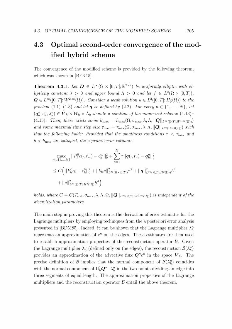
4.3. OPTIMAL CONVERGENCE OF THE MODIFIED SCHEME 205
4.3 Optimal second-order convergence of the mod-
ified hybrid scheme
The convergence of the modified scheme is provided by the following theorem,
which was shown in [BFK15].
Theorem 4.3.1. Let D ∈ L∞(Ω × [0, T ];R2×2) be uniformly elliptic with el-
lipticity constant λ > 0 and upper bound Λ > 0 and let f ∈ L2(Ω × [0, T ]),
Q ∈ L∞([0, T ];W 2,∞(Ω)). Consider a weak solution u ∈ L2([0, T ];H10 (Ω)) to the
problem (1.1)–(1.3) and let q be defined by (2.2). For every n ∈ 1, . . . , N, let
(qnh, cnh, λ
nh) ∈ V h ×Wh × Λh denote a solution of the numerical scheme (4.13)–
(4.15). Then, there exists some hmax = hmax(Ω, σmax, λ,Λ, ||Q||L∞([0,T ],W 1,∞(Ω)))
and some maximal time step size τmax = τmax(Ω, σmax, λ,Λ, ||Q||L∞(Ω×[0,T ])) such
that the following holds: Provided that the smallness conditions τ < τmax and
h < hmax are satisfied, the a priori error estimate
maxm∈1,...,N
||P 0hc(·, tm)− cmh ||20 +
N∑n=1
τ ||q(·, tn)− qnh||20
≤ C(||P 0
hc0 − c0h||20 + ||∂ttc||2L∞(Ω×[0,T ])τ
2 + ||q||2L∞([0,T ];H2(Ω))h4
+ ||c||2L∞([0,T ];H2(Ω))h4)
holds, where C = C(Tend, σmax, λ,Λ,Ω, ||Q||L∞([0,T ];W 2,∞(Ω))) is independent of the
discretization parameters.
The main step in proving this theorem is the derivation of error estimates for the
Lagrange multipliers by employing techniques from the a posteriori error analysis
presented in [BDM85]. Indeed, it can be shown that the Lagrange multiplier λnhrepresents an approximation of cn on the edges. These estimates are then used
to establish approximation properties of the reconstruction operator B. Given
the Lagrange multiplier λnh (defined only on the edges), the reconstruction B(λnh)
provides an approximation of the advective flux Qncn in the space V h. The
precise definition of B implies that the normal component of B(λnh) coincides
with the normal component of Π1hQ
n · λnh in the two points dividing an edge into
three segments of equal length. The approximation properties of the Lagrange
multipliers and the reconstruction operator B entail the above theorem.

206 CHAPTER 4. MHFE SCHEMES BASED ON THE BDM1 ELEMENT
4.4 Numerical results
In this section, we illustrate our theoretical results and compare the classical and
the modified BDM1 scheme with the help of a computational experiment. Our
numerical results show that the error bounds stated above are sharp. Further
numerical tests, in which the modified BDM1 scheme was applied to nonlinear
reactive transport problems, are presented in [BRBK12, BBKR13].
To be more precise, problem (1.1)–(1.3) is solved on the unit square Ω = (0, 1)2 ⊂R2 on the time interval J = (0, 1). For the (scalar) diffusion coefficient and the
velocity field, we choose D = 1 and Q = (0,−1)T , respectively. Moreover,
homogeneous Dirichlet conditions are imposed on the boundary ∂Ω. The source
term f is prescribed so that the analytical solution of the problem is given by
u(x, y, t) = x(1− x)y(1− y)e−t .
In each refinement step, the mesh (which initially consists of two triangles) is
uniformly refined, and the errors
E(1)h,τ = τ 1/2
(N∑n=1
‖q(·, tn)− qnh‖20
)1/2
,
E(2)h,τ = max
1≤n≤N‖c(·, tn)− cnh‖0 ,
E(3)h,τ = max
1≤n≤N‖P 0
hc(·, tn)− cnh‖0
are computed. For all computations, a fixed time step size τ = 0.001 is used,
which is sufficiently small to ensure that the time discretization error is neg-
ligible compared to the space discretization error. The experimental orders of
convergence are determined by means of
EOC(i)h,τ = log2
(E
(i)2h,τ
E(i)h,τ
), i ∈ 1, 2, 3 .
The results of the computations are listed in Tables 4.2 and 4.3. As expected,
we obtain optimal second order convergence for the flux variable if the advective
fluxes are approximated using the Lagrange multipliers, whereas only suboptimal
first order convergence is observed when the classical scheme is used. Moreover,

4.4. NUMERICAL RESULTS 207
the scalar unknowns are approximated with first order accuracy for both schemes,
the magnitude of the errors being of almost equal size. For the approximation of
the projection P 0hc of the scalar variable into the space of piecewise constants by
our numerical solution cnh, we observe the usual (second order) superconvergence
result both in the case of the classical scheme and in the case of the modified
scheme.
triangles E(1)h,τ EOC E
(2)h,τ EOC E
(3)h,τ EOC
2 · 40 4.36e-02 2.91e-02 1.80e-02
2 · 41 2.01e-02 1.12 1.60e-02 0.86 6.37e-03 1.50
2 · 42 5.94e-03 1.76 8.57e-03 0.90 1.88e-03 1.76
2 · 43 1.56e-03 1.93 4.36e-03 0.97 4.94e-04 1.93
2 · 44 3.96e-04 1.98 2.19e-03 0.99 1.24e-04 1.99
2 · 45 9.88e-05 2.00 1.10e-03 1.00 3.07e-05 2.02
2 · 46 2.39e-05 2.04 5.48e-04 1.00 7.18e-06 2.10
Table 4.2: L2-errors and experimental orders of convergence (EOC) for the mod-ified BDM1 scheme
triangles E(1)h,τ EOC E
(2)h,τ EOC E
(3)h,τ EOC
2 · 40 4.13e-02 2.91e-02 1.79e-02
2 · 41 2.05e-02 1.01 1.60e-02 0.86 6.34e-03 1.50
2 · 42 6.91e-03 1.57 8.57e-03 0.90 1.87e-03 1.76
2 · 43 2.51e-03 1.46 4.36e-03 0.97 4.91e-04 1.93
2 · 44 1.09e-03 1.21 2.19e-03 0.99 1.23e-04 1.99
2 · 45 5.19e-04 1.07 1.10e-03 1.00 3.05e-05 2.02
2 · 46 2.56e-04 1.02 5.48e-04 1.00 7.12e-06 2.10
Table 4.3: L2-errors and experimental orders of convergence (EOC) for the clas-sical BDM1 scheme

Conclusion
In the first part of this work, we developed a numerical framework for efficiently
simulating partially miscible multiphase multicomponent flow in porous media,
modeled by a system of coupled and strongly nonlinear partial differential equa-
tions, ordinary differential equations, and algebraic equations.
For this purpose, the problem was transformed with the help of a reduction
scheme, which preserves the model and allows the unknown equilibrium reac-
tion rates to be eliminated from the system. More precisely, a variant of the
reduction scheme including additional variables was used, which were shown to
be mandatory to obtain a well-conditioned global problem, cf. [HKK10, Hof10].
In contrast to the work mentioned above, we need an additional transformed
variable representing the interphase mass exchange between the liquid and the
gas phase, and there are no partial differential equations decoupling from the
rest of the system after using the reduction scheme. This is due to the nonlinear
coupling of flow and transport in our multiphase model, which implies that each
partial differential equation depends on the liquid pressure variable. If, however,
the primary variables are chosen appropriately, it remains possible to reduce the
size of the global problem by shifting at least one block of ODEs to the local
level.
In the transformed system, the algebraic equations resulting from the chemical
equilibria are eliminated with the help of a nonlinear, implicitly defined resolution
function. Hereby, the equilibrium conditions consisting of equations and inequal-
ity constraints are formulated as a complementarity problem and rewritten as
algebraic equations using the minimum function. The existence of a resolution
function is established by using the connection of the nonlinear system of alge-
braic equations to a constrained minimization problem based on a modified Gibbs
functional, and numerical strategies to evaluate it numerically are presented. This
208

CONCLUSION 209
requires a formulation based on the logarithms of the concentrations. Moreover,
we present a method to ensure that the local nonlinear solver does not produce
nonphysical values while solving the chemical subproblem. As a nonlinear solver,
the Semismooth Newton method is used, which converges locally quadratically.
The use of the resolution function corresponds to an elimination on the level of
the nonlinear solver, which can be efficiently carried out on multiple processors.
The time discretization of the system obtained after the variable transformation
and the use of the resolution function is done using the implicit Euler method,
and the spatial discretization is based on a linear finite element method, enhanced
by an upwind finite volume stabilization for advection–dominated problems.
Using a global implicit approach, the nonlinear systems that remain to be solved
in each time step are treated with Newton’s method. With the help of the
resolution function, we are ready to use a persistent set of primary variables that
are valid in either phase state and for an arbitrary mineral assemblage. Thus,
the discontinuous switch of variables during the simulation as a result of the
appearance or disappearance of the gas phase or the dissolution and precipitation
of minerals can be avoided.
Regarding the definition of primary variables, our numerical tests indicate that
the use of two extended pressure variables leads to better convergence properties
of the nonlinear solver than the use of only one pressure variable in a smaller
global system. This is because the nonlinear coefficient functions depend directly
on one primary variable if two phase pressures are used as primary variables.
Moreover, there are fewer nonlinearities in the transport operators which involve
the gradients of both phase pressures.
Different numerical tests related to hydrogen migration in deep geological repos-
itories of radioactive waste and to CO2 sequestration show that our solver, which
was designed for 2D and 3D computations and implemented in a parallel finite
element toolbox, provides accurate numerical results, and that it is capable of
handling the strongly nonlinear coupling of flow, transport, chemical reactions,
and mass transfer across the phases. If a strict stopping criterion is used for the
nonlinear solver, the global implicit approach required significantly less compu-
tation time than the sequential iterative approach.

210 CONCLUSION
The second part of this work deals with the analysis of robust mixed hybrid finite
element methods of lowest order for advection–diffusion problems. When advec-
tion strongly dominates diffusion, the standard mixed method [DR85] typically
fails to resolve steep gradients in the analytical solution and produces approx-
imations that are polluted by spurious oscillations. One of many methods to
overcome this is to employ upwinding to the method. In the approach studied
here, this is accomplished by extending the classical scheme with the help of the
Lagrange multipliers that arise from the hybrid problem formulation. It relies
on the fact that the Lagrange multipliers represent approximations of the scalar
unknown on the interelement boundaries and uses them in the approximation of
the advective fluxes. Using techniques from the a posteriori error analysis, we are
able to establish optimal order convergence for a new class of methods including
the standard method, a partial upwind method, and a full upwind method. The
advantage of the specific choice of the upwind weights is the fact that the method
remains local such that static condensation can still be employed, whereas the
standard upwind-mixed method requires information from neighbor cells such
that static condensation is no longer applicable.
Concerning approximations with the BDM1 mixed finite element, we show that
the use of Lagrange multipliers in the discretization of the advective term pro-
vides optimal second order convergence for the total flux variable consisting of
advective and diffusive flux in the L2 norm, whereas the standard mixed method
is known to be of suboptimal first order accuracy only. Thus, the modification,
which was intended to enhance the robustness of the standard method against
advection–dominance for moderately advection dominated problems, leads to a
higher accuracy of the method without increasing the computational costs.

Bibliography
[AB85] D. N. Arnold and F. Brezzi. Mixed and nonconforming fi-nite element methods: implementation, postprocessing and er-ror estimates. R.A.I.R.O. Modelisation mathematique et analysenumerique, 19(1):7–32, 1985.
[ACC+11] O. Angelini, C. Chavant, E. Chenier, R. Eymard, and S. Granet.Finite volume approximation of a diffusion–dissolution model andapplication to nuclear waste storage. Mathematics and Computersin Simulation, 81(10):2001–2017, 2011.
[AK10] L. Amir and M. Kern. A global method for coupling transportwith chemistry in heterogeneous porous media. Computational Geo-sciences, 14(3):465–481, 2010.
[AKV15] E. Ahusborde, M. Kern, and V. Vostrikov. Numerical simulationof two-phase multicomponent flow with reactive transport in porousmedia: application to geological sequestration of CO2. ESAIM: Pro-ceedings and Surveys, 50:21–39, 2015.
[AP09] A. Abadpour and M. Panfilov. Method of Negative Saturationsfor Modeling Two-phase Compositional Flow with OversaturatedZones. Transport in Porous Media, 79(2):197–214, 2009.
[BBD+08] D. Boffi, F. Brezzi, L. F. Demkowicz, R. G. Duran, R. S. Falk,and M. Fortin. Mixed Finite Elements, Compatibility Conditions,and Applications, volume 1939 of Lecture Notes in Mathematics.Springer, 2008. Lectures given at the C.I.M.E. Summer School heldin Cetraro, June 26–July 1, 2006. Edited by D. Boffi and L. Gastaldi.
[BBF13] D. Boffi, F. Brezzi, and M. Fortin. Mixed Finite Element Methodsand Applications. Springer, Berlin, 2013.
[BBKR13] M. Bause, F. Brunner, P. Knabner, and F. A. Radu. An ImprovedOptimal Order Mixed Finite Element Method for Semilinear Trans-port Problems. In A. Cangiani, R. L. Davidchack, E. Georgoulis,
211

212 BIBLIOGRAPHY
A. N. Gorban, J. Levesley, and M. V. Tretyakov, editors, NumericalMathematics and Advanced Applications 2011, pages 247–255, 2013.
[BC64] R. H. Brooks and A. T. Corey. Hydraulic Properties of PorousMedia. In Hydrology Papers. Colorado State University, 1964.
[BDM85] F. Brezzi, J. Douglas, Jr., and L. D. Marini. Two families of mixedfinite elements for second order elliptic problems. Numerische Math-ematik, 47(2):217–235, 1985.
[Bea72] J. Bear. Dynamics of Fluids in Porous Media. Elsevier, New York,1972.
[Bet96] C. Bethke. Geochemical Reaction Modeling: Concepts and applica-tions. Oxford University Press, New York, 1996.
[BF91] F. Brezzi and M. Fortin. Mixed and Hybrid Finite Element Methods,no. 15 in Springer Series in Computational Mathematics. Springer,New York, 1991.
[BFK14] F. Brunner, F. Frank, and P. Knabner. FV Upwind Stabiliza-tion of FE Discretizations for Advection–Diffusion Problems. InJ. Fuhrmann, M. Ohlberger, and C. Rohde, editors, Finite Volumesfor Complex Applications VII–Methods and Theoretical Aspects, vol-ume 77 of Springer Proceedings in Mathematics & Statistics, pages177–185. Springer International Publishing, 2014.
[BFK15] F. Brunner, J. Fischer, and P. Knabner. Analysis of a modifiedsecond-order mixed hybrid BDM1 finite element method for trans-port problems in divergence form. Submitted, 2015.
[BG12] I. Ben Gharbia and J. C. Gilbert. Nonconvergence of the plainNewton-min algorithm for linear complementarity problems with aP-matrix. Mathematical Programming, 134(2):349–364, 2012.
[BGS13] A. Bourgeat, S. Granet, and F. Smaı. Compositional two-phaseflow in saturated-unsaturated porous media: benchmarks for phaseappearance/disappearance. In P. Bastian, J. Kraus, R. Scheichl, andM. Wheeler, editors, Simulation of Flow in Porous Media, volume 12of Radon Series on Computational and Applied Mathematics, pages81–106. Walter de Gruyter, 2013.
[Bie06] A. Bielinski. Numerical Simulation of CO2 Sequestration in Geolog-ical Formations. PhD thesis, Institut fur Wasser- und Umweltsys-temmodellierung. Universitat Stuttgart, 2006.

BIBLIOGRAPHY 213
[BJ14] I. Ben Gharbia and J. Jaffre. Gas phase appearance and disappear-ance as a problem with complementarity constraints. Mathematicsand Computers in Simulation, 99:28–36, 2014.
[BJS09] A. Bourgeat, M. Jurak, and F. Smaı. Two-phase, partially miscibleflow and transport modeling in porous media; application to gasmigration in a nuclear waste repository. Computational Geosciences,13(1):29–42, 2009.
[BJS13] A. Bourgeat, M. Jurak, and F. Smaı. On persistent primary vari-ables for numerical modeling of gas migration in a nuclear wasterepository. Computational Geosciences, 17(2):287–305, 2013.
[BKKK11] H. Buchholzer, C. Kanzow, P. Knabner, and S. Krautle. The semis-mooth Newton method for the solution of reactive transport prob-lems including mineral precipiation-dissolution reactions. Computa-tional Optimization and Applications, 50(2):193–221, 2011.
[BRBK12] F. Brunner, F. A. Radu, M. Bause, and P. Knabner. Optimal orderconvergence of a modified BDM1 mixed finite element scheme forreactive transport in porous media. Advances in Water Resources,35:163–171, 2012.
[BRK14] F. Brunner, F. A. Radu, and P. Knabner. Analysis of an upwind-mixed hybrid finite element method for transport problems. SIAMJournal on Numerical Analysis, 52(1):83–102, 2014.
[Bru10] F. Brunner. Hybride gemischte Finite Elemente fur Systeme vonTransportreaktionsgleichungen in porosen Medien: AlgorithmischeUmsetzung und Simulation von 2D-Szenarien. Diplomarbeit, FAUErlangen-Nurnberg, 2010.
[BV04] S. Boyd and L. Vandenberghe. Convex Optimization. CambridgeUniversity Press, 2004.
[CGCM74] K. H. Coats, W. D. George, C. Chu, and B. E. Marcum. Three-Dimensional Simulation of Steamflooding. Society of Petroleum En-gineers Journal, 14(6):573–592, 1974.
[CHB02] H. Class, R. Helmig, and P. Bastian. Numerical simulation of non-isothermal multiphase multicomponent processes in porous media.:1. An efficient solution technique. Advances in Water Resources,25(5):533–550, 2002.
[CHK+10] J. Carrayrou, J. Hoffmann, P. Knabner, S. Krautle, C. deDieuleveult, J. Erhel, J. van der Lee, V. Lagneau, K. U. Mayer,

214 BIBLIOGRAPHY
and K. T. B. MacQuarrie. Comparison of numerical methodsfor simulating strongly nonlinear and heterogeneous reactive trans-port problems—the MoMaS benchmark case. Computational Geo-sciences, 14(3):483–502, 2010.
[CKK10] J. Carrayrou, M. Kern, and P. Knabner. Reactive transport bench-mark of MoMaS. Computational Geosciences, 14(3):385–392, 2010.
[Cla83] F. H. Clarke. Optimization and Nonsmooth Analysis. Wiley, NewYork, 1983.
[CMB02] J. Carrayrou, R. Mose, and P. Behra. New efficient algorithm forsolving thermodynamic chemistry. American Institute of ChemicalEngineers Journal, 48(4):894–904, 2002.
[DA99] C. Dawson and V. Aizinger. Upwind-mixed methods for transportequations. Computational Geosciences, 3(2):93–110, 1999.
[Daw91] C. Dawson. Godunov-mixed methods for advective flow problemsin one space dimension. SIAM Journal on Numerical Analysis,28(5):1282–1309, 1991.
[Daw93] C. Dawson. Godunov-mixed methods for advection-diffusion equa-tions in multidimensions. SIAM Journal on Numerical Analysis,30(5):1315–1332, 1993.
[Daw98] C. Dawson. Analysis of an upwind-mixed finite element methodfor nonlinear contaminant transport equations. SIAM Journal onNumerical Analysis, 35(5):1709–1724, 1998.
[dC15] R. de Cuveland. Two-Phase Compositional Flow Simulation withPersistent Variables. PhD thesis, Universitat Heidelberg, 2015.
[dDE10] C. de Dieuleveult and J. Erhel. A global approach to reactive trans-port: application to the MoMaS benchmark. Computational Geo-sciences, 14(3):451–464, 2010.
[dDEK09] C. de Dieuleveult, J. Erhel, and M. Kern. A global strategy forsolving reactive transport equations. Journal of ComputationalPhysics, 228(17):6395–6410, 2009.
[Dem02] A. Demlow. Suboptimal and optimal convergence in mixed finite el-ement methods. SIAM Journal on Numerical Analysis, 39(6):1938–1953, 2002.

BIBLIOGRAPHY 215
[Dem04] A. Demlow. Localized pointwise error estimates for mixed finiteelement methods. Mathematics of Computation, 73(248):1623–1653,2004.
[Deu11] P. Deuflhard. Newton methods for nonlinear problems: affine invari-ance and adaptive algorithms, volume 35 of Springer Series in Com-putational Mathematics. Springer, Berlin, Heidelberg, New York,2011.
[dLFK00] T. de Luca, F. Facchinei, and C. Kanzow. A Theoretical and Nu-merical Comparison of Some Semismooth Algorithms for Comple-mentarity Problems. Computational Optimization and Applications,16(2):173–205, 2000.
[DMW92] Z. Duan, N. Møller, and J. H. Weare. An equation of state for theCH4-CO2-H2O system: I. Pure systems from 0 to 1000 C and 0to 8000 bar. Geochimica et Cosmochimica Acta, 56(7):2605–2617,1992.
[DPvDC08] V. M. Devigne, I. S. Pop, C. J. van Duijn, and T. Clopeau. Anumerical scheme for the pore-scale simulation of crystal dissolutionand precipitation in porous media. SIAM Journal on NumericalAnalysis, 46(2):895–919, 2008.
[DR82] J. Douglas, Jr. and J. E. Roberts. Mixed finite element methods forsecond order elliptic problems. Matematica Aplicada e Computa-cional, 1(1):91–103, 1982.
[DR85] J. Douglas, Jr. and J. E. Roberts. Global estimates for mixed meth-ods for second order elliptic equations. Mathematics of Computation,44(169):39–52, 1985.
[DS03] Z. Duan and R. Sun. An improved model calculating CO2 solubilityin pure water and aqueous NaCl solutions from 273 to 533 K andfrom 0 to 2000 bar. Chemical Geology, 193(3–4):257–271, 2003.
[Dur88] R. G. Duran. Error analysis in Lp, 1 ≤ p ≤ ∞, for mixedfinite element methods for linear and quasi-linear elliptic prob-lems. R.A.I.R.O. Modelisation mathematique et analyse numerique,22(3):371–387, 1988.
[FDT12] Y. Fan, L. J. Durlofsky, and H. Tchelepi. A fully-coupled flow-reactive-transport formulation based on element conservation, withapplication to CO2 storage simulations. Advances in Water Re-sources, 42:47–61, 2012.

216 BIBLIOGRAPHY
[Fet93] C. W. Fetter. Contaminant Hydrogeology. Macmillan PublishingCompany, New York, 1993.
[FR92] J. C. Friedly and J. Rubin. Solute transport with multipleequilibrium-controlled or kinetically controlled chemical reactions.Water Resources Research, 28(7):1935–1953, 1992.
[Fri91] J. C. Friedly. Extent of reaction in open systems with multipleheterogeneous reactions. American Institute of Chemical EngineersJournal, 37(5):687–693, 1991.
[FS91] P. A. Forsyth and R. B. Simpson. A two-phase, two-componentmodel for natural convection in a porous medium. InternationalJournal for Numerical Methods in Fluids, 12(7):655–682, 1991.
[FWV98] A. Fenghour, W. A. Wakeham, and V. Vesovic. The viscosity ofcarbon dioxide. Journal of Physical and Chemical Reference Data,27(1):31–44, 1998.
[Gar01] J. E. Garcıa. Density of Aqueous Solutions of CO2. Lawrence Berke-ley National Laboratory, 2001.
[GK02] C. Geiger and C. Kanzow. Theorie und Numerik restringierter Op-timierungsaufgaben. Springer, Berlin, Heidelberg, 2002.
[GNC09] S. E. Gasda, J. M. Nordbotten, and M. A. Celia. Vertical equilibriumwith subscale analytical methods for geological CO2 sequestration.Computational Geosciences, 13(4):469–481, 2009.
[GNC11] S. E. Gasda, J. M. Nordbotten, and M. A. Celia. Vertically aver-aged approaches for CO2 migration with solubility trapping. WaterResources Research, 47(5), 2011.
[Hel97] R. Helmig. Multiphase Flow and Transport Processes in the Sub-surface: A Contribution to the Modeling of Hydrosystems. Springer,Berlin, Heidelberg, 1997.
[HIK03] M. Hintermuller, K. Ito, and K. Kunisch. The primal-dual activeset strategy as a semismooth newton method. SIAM Journal onOptimization, 13(3):865–888, 2003.
[HKK10] J. Hoffmann, S. Krautle, and P. Knabner. A parallel global–implicit2-D solver for reactive transport problems in porous media based ona reduction scheme and its application to the MoMaS benchmarkproblem. Computational Geosciences, 14(3):421–433, 2010.

BIBLIOGRAPHY 217
[HKK12] J. Hoffmann, S. Krautle, and P. Knabner. A general reductionscheme for reactive transport in porous media. Computational Geo-sciences, 16(4):1081–1099, 2012.
[HLL07] G. Hammond, P. Lichtner, and C. Lu. Subsurface multiphaseflow and multicomponent reactive transport modeling using high-performance computing. Journal of Physics: Conference Series,78(1):012025, 2007.
[Hof10] J. Hoffmann. Reactive Transport and Mineral Dissolu-tion/Precipitation in Porous Media: Efficient Solution Algorithms,Benchmark Computations and Existence of Global Solutions. PhDThesis, Friedrich-Alexander-Universitat Erlangen-Nurnberg, 2010.
[HSN12] Y. Hao, Y. Sun, and J. J. Nitao. Overview of NUFT: A VersatileNumerical Model for Simulating Flow and Reactive Transport inPorous Media. In F. Zhang, G.-T. Yeh, and J. C. Parker, editors,Groundwater Reactive Transport Models, pages 212–239. BenthamScience Publishers, 2012.
[IEA14] IEA. Key World Energy Statistics 2014, 2014.URL: http://dx.doi.org/10.1787/key energ stat-2014-en.
[JJ96] Y. Jin and W. A. Jury. Characterizing the dependence of gas dif-fusion coefficient on soil properties. Soil Science Society of AmericaJournal, 60(1):66–71, 1996.
[JS10] J. Jaffre and A. Sboui. Henry’ law and gas phase disappearance.Transport in Porous Media, 82(3):521–526, 2010.
[KA03] P. Knabner and L. Angermann. Numerical Methods for Elliptic andParabolic Partial Differential Equations. Springer, New York, 2003.
[KK05] S. Krautle and P. Knabner. A new numerical reduction scheme forfully coupled multicomponent transport-reaction problems in porousmedia. Water Resources Research, 41(9), 2005.
[KK07] S. Krautle and P. Knabner. A reduction scheme for coupled multi-component transport-reaction problems in porous media: General-ization to problems with heterogeneous equilibrium reactions. WaterResources Research, 43(3), 2007.
[Kra08] S. Krautle. General multi-species reactive transport problems inporous media: Efficient numerical approaches and existence ofglobal solutions. Habilitation thesis, Friedrich-Alexander-UniversitatErlangen-Nurnberg, 2008.
218 BIBLIOGRAPHY
[Kra11] S. Krautle. The semismooth Newton method for multicomponentreactive transport with minerals. Advances in Water Resources,34(1):137–151, 2011.
[KvDH95] P. Knabner, C. J. van Duijn, and S. Hengst. An analysis of crystaldissolution fronts in flows through porous media. Part 1: Compatibleboundary conditions. Advances in Water Resources, 18(3):171–185,1995.
[LHHW11] A. Lauser, C. Hager, R. Helmig, and B. Wohlmuth. A new approachfor phase transitions in miscible multi-phase flow in porous media.Advances in Water Resources, 34(8):957–966, 2011.
[Li05] X. S. Li. An Overview of SuperLU: Algorithms, Implementation,and User Interface. ACM Transactions on Mathematical Software,31(3):302–325, 2005.
[LSO96] P. C. Lichtner, C. I. Steefel, and E. H. Oelkers, editors. ReactiveTransport in Porous Media, volume 34 of Reviews in Mineralogy.Mineralogical Society of America, 1996.
[LSU68] O. A. Ladyzenskaja, V. A. Solonnikov, and N. N. Ural’ceva. Linearand Quasi-linear Equations of Parabolic Type. American Mathemat-ical Society, 1968.
[MCAS04] S. Molins, J. Carrera, C. Ayora, and M. W. Saaltink. A formulationfor decoupling components in reactive transport problems. WaterResources Research, 40(10), 2004.
[MDdC+05] B. Metz, O. Davidson, H. C. de Coninck, M. Loos, and L. Meyer, ed-itors. IPCC Special Report on Carbon Dioxide Capture and Storage.Prepared by Working Group III of the Intergovernmental Panel onClimate Change, volume 4. Cambridge University Press, Cambridge,New York, 2005.
[MK14] E. Marchand and P. Knabner. Results of the MoMaS benchmark forgas phase appearance and disappearance using generalized MHFE.Advances in Water Resources, 73:74–96, 2014.
[MLLH07] R. T. Mills, C. Lu, P. Lichtner, and G. E. Hammond. Simulatingsubsurface flow and transport on ultrascale computers using PFLO-TRAN . Journal of Physics: Conference Series, 78(1):012051, 2007.
[MMK12] E. Marchand, T. Muller, and P. Knabner. Fully coupled gener-alised hybrid-mixed finite element approximation of two-phase two-component flow in porous media. Part II: numerical scheme andnumerical results. Computational Geosciences, 16(3):691–708, 2012.

BIBLIOGRAPHY 219
[MMK13] E. Marchand, T. Muller, and P. Knabner. Fully coupled general-ized hybrid-mixed finite element approximation of two-phase two-component flow in porous media. Part I: formulation and propertiesof the mathematical model. Computational Geosciences, 17(2):431–442, 2013.
[MoM10] MoMaS, 2010. URL:https://www.ljll.math.upmc.fr/cances/gdrmomas/Benchmark/multiphase/multiphasique.html .
[MQ61] R. J. Millington and J. P. Quirk. Permeability of porous solids.Transactions of the Faraday Society, 57:1200–1207, 1961.
[MSS01] S. Micheletti, R. Sacco, and F. Saleri. On some mixed finite elementmethods with numerical integration. SIAM Journal on ScientificComputing, 23(1):245–270, 2001.
[NBI13] R. Neumann, P. Bastian, and O. Ippisch. Modeling and simulation oftwo-phase two-component flow with disappearing nonwetting phase.Computational Geosciences, 17(1):139–149, 2013.
[NC12] J. M. Nordbotten and M. A. Celia. Geological Storage of CO2: Mod-eling Approaches for Large-Scale Simulation. Wiley, 2012.
[oCC11] United Nations Framework Convention on Climate Change. Re-port of the Conference of the Parties on its sixteenth ses-sion, held in Canun from 29 November to 10 December2010. Addendum. Part two: Action taken by the Confer-ence of the Parties at its sixteenth session., 2011. URL:http://unfccc.int/bodies/body/6383/php/view/reports.php.
[PP14] M. Panfilov and I. Panfilova. Method of negative saturations forflow with variable number of phases in porous media: extensionto three-phase multi-component case. Computational Geosciences,18(3):385–399, 2014.
[PR10] M. Panfilov and M. Rasoulzadeh. Interfaces of Phase Transitionand Disappearance and Method of Negative Saturation for Compo-sitional Flow with Diffusion and Capillarity in Porous Media. Trans-port in Porous Media, 83(1):73–98, 2010.
[RS97] D. Ralph and S. Scholtes. Sensitivity analysis of composite piecewisesmooth equations. Mathematical Programming, 76(3):593–612, 1997.
[RSH+11] F. A. Radu, N. Suciu, J. Hoffmann, A. Vogel, O. Kolditz, C.-H. Park,and S. Attinger. Accuracy of numerical simulations of contaminant

220 BIBLIOGRAPHY
transport in heterogeneous aquifers: A comparative study. Advancesin Water Resources, 34(1):47–61, 2011.
[RT77] P. A. Raviart and J. M. Thomas. A mixed finite element methodfor 2-nd order elliptic problems. In I. Galligani and E. Magenes, ed-itors, Mathematical Aspects of Finite Element Methods, volume 606of Lecture Notes in Mathematics, pages 292–315. Springer, Berlin,Heidelberg, 1977.
[RT91] J. E. Roberts and J. M. Thomas. Mixed and hybrid methods. Hand-book of numerical analysis, 2:523–639, 1991.
[SCA00] M. W. Saaltink, J. Carrera, and C. Ayora. A comparison of twoapproaches for reactive transport modelling. Journal of GeochemicalExploration, 69–70:97–101, 2000.
[SP05] N. Spycher and K. Pruess. CO2-H2O mixtures in the geologicalsequestration of CO2. II. Partitioning in chloride brines at 12–100 Cand up to 600 bar. Geochimica et Cosmochimica Acta, 69(13):3309–3320, 2005.
[SS97] R. Sacco and F. Saleri. Stabilization of Mixed Finite Elements forConvection-Diffusion Problems. CWI Quarterly, 10(3–4):301–315,1997.
[SS01] A. A. Shapiro and E. H. Stenby. Thermodynamics of the multicom-ponent vapor–liquid equilibrium under capillary pressure difference.Fluid Phase Equilibria, 178(1–2):17–32, 2001.
[SVG+13] M. W. Saaltink, V. Vilarrasa, F. De Gaspari, O. Silva, J. Carrera,and T. S. Rotting. A method for incorporating equilibrium chemicalreactions into multiphase flow models for CO2 storage. Advances inWater Resources, 62:431–441, 2013.
[vDK97] C. J. van Duijn and P. Knabner. Travelling wave behaviour of crys-tal dissolution in porous media flow. European Journal of AppliedMathematics, 8(1):49–72, 1997.
[vDKS98] C. J. van Duijn, P. Knabner, and R. J. Schotting. An analysisof crystal dissolution fronts in flows through porous media. part 2:incompatible boundary conditions. Advances in Water Resources,22(1):1–16, 1998.
[vDP04] C. J. van Duijn and I. S. Pop. Crystal dissolution and precipitationin porous media: Pore scale analysis. Journal fur die reine undangewandte Mathematik, 577:171–211, 2004.

BIBLIOGRAPHY 221
[vG80] M. T. van Genuchten. A closed-form equation for predicting thehydraulic conductivity of unsaturated soils. Soil Science Society ofAmerica Journal, 44(5):892–898, 1980.
[VM92] A. J. Valocchi and M. Malmstead. Accuracy of operator splitting foradvection-dispersion-reaction problems. Water Resources Research,28(5):1471–1476, 1992.
[Voh07] M. Vohralik. A posteriori error estimates for lowest-order mixedfinite element discretizations of convection-diffusion-reaction equa-tions. SIAM Journal on Numerical Analysis, 45(4):1570–1599, 2007.
[WBM+12] M. D. White, D. H. Bacon, B. P. McGrail, D. J. Watson, S. K.White, and Z. F. Zhang. STOMP Subsurface Transport Over Mul-tiple Phases: STOMP-CO2 and STOMP-CO2e Guide: Version 1.0.Technical report, Pacific Northwest National Laboratory, Richland,Washington, 2012.
[WF12] M. D. White and Y. Fang. STOMP-ECKEChem: An engineeringperspective on reactive transport in geologic media. In F. Zhang, G.-T. Yeh, and J. C. Parker, editors, Groundwater Reactive TransportModels, pages 112–140. Bentham Science Publishers, 2012.
[Wie] Christian Wieners. M++ (meshes, multigrid and more).http://www.math.kit.edu/ianm3/seite/mplusplus.
[Wie05] C. Wieners. Distributed point objects. a new concept for parallel fi-nite elements. In J. T. Barth, M. Griebel, D. E. Keyes, R. M. Niem-inen, D. Roose, T. Schlick, R. Kornhuber, R. Hoppe, J. Periaux,P. Pironneau, O. Widlund, and J. Xu, editors, Domain Decompo-sition Methods in Science and Engineering, volume 40 of LectureNotes in Computational Science and Engineering, pages 175–182.Springer, Berlin, Heidelberg, 2005.
[Wie10] C. Wieners. A geometric data structure for parallel finite elementsand the application to multigrid methods with block smoothing.Computing and Visualization on Science, 13(4):161–175, 2010.
[WM89] C. H. Whitson and M. L. Michelsen. The negative flash. Fluid PhaseEquilibria, 53:51–71, 1989.
[XSS+12] T. Xu, E. Sonnenthal, N. Spycher, G. Zhang, L. Zheng, andK. Pruess. TOUGHREACT: A Simulation Program for Subsur-face Reactive Chemical Transport under Non-isothermal MultiphaseFlow Conditions. In F. Zhang, G.-T. Yeh, and J. C. Parker, editors,

222 BIBLIOGRAPHY
Groundwater Reactive Transport Models, pages 74–95. Bentham Sci-ence Publishers, 2012.
[YAD10] A. Younes, P. Ackerer, and F. Delay. Mixed finite elements forsolving 2-D diffusion-type equations. Reviews of Geophysics, 48(1),2010.
[YT89] G.-T. Yeh and V. S. Tripathi. A critical evaluation of recent de-velopments in hydrogeochemical transport models of reactive mul-tichemical components. Water Resources Research, 25(1):93–108,1989.