multiphysics computational models for cardiac flow - mechanical

INTERNATIONAL JOURNAL FOR NUMERICAL METHODS IN BIOMEDICAL ENGINEERINGInt. J. Numer. Meth. Biomed. Engng. (2013)Published online in Wiley Online Library (wileyonlinelibrary.com). DOI: 10.1002/cnm.2556

Multiphysics computational models for cardiac flow andvirtual cardiography

Jung Hee Seo, Vijay Vedula, Theodore Abraham and Rajat Mittal*,†

Johns Hopkins University, 3400 N Charles St, Baltimore, MD 21218, USA

SUMMARY

A multiphysics simulation approach is developed for predicting cardiac flows as well as for conductingvirtual echocardiography (ECHO) and phonocardiography (PC) of those flows. Intraventricular blood flowin pathological heart conditions is simulated by solving the three-dimensional incompressible Navier–Stokesequations with an immersed boundary method, and using this computational hemodynamic data, echocar-diographic and phonocardiographic signals are synthesized by separate simulations that model the physicsof ultrasound wave scattering and flow-induced sound, respectively. For virtual ECHO, a Doppler ultra-sound image is reproduced through Lagrangian particle tracking of blood cell particles and application ofsound wave scattering theory. For virtual PC, the generation and propagation of blood flow-induced sounds(‘hemoacoustics’) is directly simulated by a computational acoustics model. The virtual ECHO is applied toreproduce a color M-mode Doppler image for the left ventricle as well as continuous Doppler image for theoutflow tract of the left ventricle, which can be verified directly against clinically acquired data. The potentialof the virtual PC approach for providing new insights between disease and heart sounds is demonstrated byapplying it to modeling systolic murmurs caused by hypertrophic cardiomyopathy. Copyright © 2013 JohnWiley & Sons, Ltd.

Received 12 November 2012; Revised 11 February 2013; Accepted 8 April 2013

KEY WORDS: hemodynamics; hemoacoustics; echocardiography; phonocardiography; computationalfluid dynamics; Doppler ultrasound; hypertrophic cardiomyopathy; systolic murmur

1. INTRODUCTION

Computational modeling has increasingly become the tool of choice for studying cardiac flows[1–6]. Computational modeling of hemodynamics enables a comprehensive analysis of flow, pres-sure, vorticity, and other flow related metrics in normal as well as diseased hearts and, in doingso, may reveal the significance of flow structures for ventricular function. The future of computa-tional hemodynamics is the simulation of flows in patient-specific models (e.g. [2, 4]) for improveddiagnostic assessment and modeling assisted treatment and surgery.

A number of issues and challenges exist in order to achieve this promise of computational hemo-dynamics of cardiac flows. This paper deals with two of these challenges: the first one is the need formethods to rapidly assess the validity of the computational result for a patient-specific simulation. Itshould be noted that although simulations of cardiac flows can be validated and verified for canoni-cal (benchtop) models, the translation of these models into clinical practice will require revalidationfor each and every patient. This is primarily because the input data (such as inflow/outflow con-ditions) obtained from the patient specific measurements for the simulation oftentimes are limitedand some of these need to be estimated or modeled. Thus, the overall accuracy of the computationalresult for every patient-specific model needs to be validated prior to using the simulation data for

*Correspondence to: Rajat Mittal, Johns Hopkins University, 3400 N Charles St, Baltimore, MD 21218, USA.†E-mail: [email protected]

Copyright © 2013 John Wiley & Sons, Ltd.

J. H. SEO ET AL.

diagnosis and treatment. The second issue addressed here is the connection between the compu-tational hemodynamic results and the diagnostic data used in the clinical field. Although the flowfeatures and vortical structures can be investigated in detail with the computational hemodynamics,it is currently difficult to use this information directly for the diagnosis and treatment for the heartdiseases. Therefore, it may be important to develop correlations between specific features of cardiacflows (as extracted from computational fluid dynamics (CFD)) and the clinical data that are availablefor diagnosis of cardiac function.

The aforementioned two issues can be addressed by generating ‘virtual’ cardiographies using thecomputational hemodynamic results of cardiac flows. In this study, we describe a multiphysics sim-ulation approach for the modeling of cardiac flows as well as virtual echocardiography (ECHO)and phonocardiography (PC). Cardiac ECHO employs Doppler ultrasound for the assessment ofintracardiac flows (e.g., [7–9]), and PC employs recording and analysis of heart sounds for auscul-tation [10–13]. Both ECHO and PC are noninvasive and inexpensive diagnostic methods for cardiacdisease and oftentimes used to diagnose and assess heart conditions including but not limited todiastolic dysfunction, valvular disease, congenital disorders, and cardiomyopathies. For example,the early/atrial filling wave velocity ratio (E/A ratio) measured by the pulsed wave (PW) Doppler[8] and the flow propagation velocity extracted from the color M-mode Doppler diagram [14] areused to assess the health of the ventricle. In addition to this, continuous wave (CW) Doppler isapplied to check the severity of aortic stenosis or sub-aortic obstacle based on the maximum bloodflow velocity in the outflow tract [9]. At the same time, the blood flow in the ventricle with diastolicdysfunction (e.g., very high (>>1) or low (<<1) E/A ratios) causes additional heart sounds suchas the so-called S3 and S4 sounds [13], and heart murmur [10] is generated by abnormal bloodflows associated with aortic stenosis, obstructive hypertrophic cardiomyopathy (HCM), and mitralregurgitation.

All the diagnostic metrics extracted from ECHO Doppler investigation and abnormal heart soundsare directly related to the blood flow dynamics in the ventricle. Thus, virtual ECHO and PC canserve as a bridge between clinical data and computational hemodynamic results. In the presentstudy, intraventricular blood flows for left ventricles (LVs) with pathological conditions (diastolicdysfunction, HCM) are simulated via CFD, and echocardiographic and phonocardiographic dataare synthesized by separate simulations that model the physics of ultrasound wave scattering andflow-induced sound, respectively. These ‘virtual’ ECHO and PC provide data that can be compareddirectly with clinically acquired data. In particular, these virtual ECHO and PC can be used forrapid validation of computational results by comparing to the actual cardiographic data, and fur-thermore, such comparisons will allow us to calibrate a given patient-specific, computational heartmodel. The virtual cardiography will also improve our ability to interpret the cardiac flow simula-tion data. It is expected that the development of detailed correlations between blood flow dynamicsand the cardiographic data will provide valuable information for the improvement of diagnostictools based on these modalities. The simulation methods are described in Section 2, and in Section 3,we describe the simulations of blood flow inside LV with severe diastolic dysfunction and the asso-ciated mitral inflow Doppler and color M-mode Doppler. We also describe virtual modeling of CWDoppler measurements for the LV outflow tract and the systolic ejection murmur associated withobstructive HCM.

2. METHODS

In the present study, intraventricular blood flow is simulated by solving the three-dimensionalincompressible Navier–Stokes equations with an immersed boundary method [15]. Using this com-putational hemodynamic result, virtual echocardiographies and phonocardiographies are generatedvia separate simulations that model the physics of ultrasound wave scattering and flow-inducedsound, respectively. For virtual ECHO, we generate Doppler ultrasound images which depictsintraventricular flow motions. This is carried out by Lagrangian tracking of particles and apply-ing sound wave scattering theory [16] to these particles. The Lagrangian particles represent virtualred blood cells (RBCs) that are primarily responsible for the backscatter of ultrasound from blood.The motion of virtual RBC particles is tracked by using the time-dependant Eulerian velocity field

Copyright © 2013 John Wiley & Sons, Ltd. Int. J. Numer. Meth. Biomed. Engng. (2013)DOI: 10.1002/cnm

MULTIPHYSICS COMPUTATIONAL MODELS

obtained from the cardiac flow simulation, and ultrasound wave propagation and scattering by RBCparticles are described by an acoustic analogy for arbitrary transducer/receiver shape. Once the timeseries of scattered ultrasound signal is obtained on the receiver, a Doppler ultrasound image can beconstructed by a signal processing approach.

For virtual PC, we simulate the blood flow-induced sound generation and propagation(‘hemoacoustics’) using a hybrid approach that employs the incompressible Navier–Stokes and thelinearized perturbed compressible equations (LPCE) [17]. The sound source term in this approachis obtained from the computational hemodynamic simulation, and the sound propagation throughthe thorax is modeled with a structural wave equation.

2.1. Computational hemodynamics

For the intraventricular blood flows, blood is assumed to be a Newtonian fluid and thus its motionis governed by the incompressible Navier–Stokes equations;

r � EU D 0,@ EU

@tC . EU � r/ EU C

1

�0r EP D �0r

2 EU , (1)

where EU is a velocity vector, P is a pressure, and �0 and �0 are the density and kinematic viscosityof the blood. Equation (1) is solved by a fractional step method [18];

EU � � EU n

�tD1

2

h�. EU � r/ EU C �0r

2 EUi�C1

2

h�. EU � r/ EU C �0r

2 EUin

, (2)

r2P nC1 D�0

�tr � EU � (3)

EU nC1 D EU � ��t

�0rP nC1 (4)

where EU � is a intermediate velocity field and superscript n denotes the time level. The advection–diffusion equation, Equation (2), is computed by a second-order Crank–Nicolson method, and thepressure Poisson equation, Equation (3), is solved by a geometric multi-grid method [19]. All thespatial derivatives are discretized by a second-order central differencing. The discretized equationsare solved on the nonbody conformal Cartesian grid and the complex, moving boundaries are treatedby a sharp-interface immersed boundary method as described in Ref. [15]. In this method, the endo-cardial surface is represented by an unstructured mesh with triangular elements, and this surface isimmersed into the Cartesian volume grid. The key difference between the present immersed bound-ary method and the previous work of Peskin and coworkers [20, 21] is that the boundary conditionon the immersed body surface is directly imposed by assigning the variable value on the ‘Ghost cell’(the cell in the nonfluid region adjacent to the fluid cell) rather than applying a distributed forcingterm on the momentum equation (Equation (2)). Also, we do not solve the elastic fiber equationsfor the myocardium. In the present study, the endocardial surface moves with a prescribed velocity,and the boundary conditions for the flow field on the surface are imposed by a multi-dimensionalghost-cell method. Further details of the present immersed boundary flow solver can be found inthe Ref. [15].

2.2. Blood cell particle tracking

The motion of ‘virtual’ RBCs is simulated by the Lagrangian particle tracking algorithm. The par-ticles that represent the RBC are randomly distributed in the blood flow domain, and their motion istracked by the equation

Exp.t C�t/D Exp.t/C

Z tC�t

t

EU .Exp/ dt , (5)


J. H. SEO ET AL.

where Exp is the particle position vector and EU .Ex/ is the Eulerian velocity vector field obtainedfrom the full Navier–Stokes computation. The velocity at the particle position is computed bya tri-linear interpolation and the time integration of Equation (5) is performed by a four-stageRunge–Kutta method.

2.3. Doppler ultrasound modeling

In this study, we model the scattering of ultrasound wave by each RBC as proposed by Oung andForsberg [16]. The schematic diagram is shown in Figure 1. The ultrasound wave emitted from thetransducer surface (S1/ propagates to the moving RBC particle and the wave scattered by the parti-cle is received by the receiver surface (S2/. Note that two surfaces S1 and S2 can be the same. Theultrasound wave emitted by a transducer of arbitrary shape can be modeled by a Green’s functionsolution [22] as

.Ex, t /D1

2�

ZS

1

re.t � r=c/dS , (6)

where is a velocity potential of the sound wave, r is the distance from the point on the transducersurface to Ex, c is the speed of sound, and e.t/ is the surface normal velocity fluctuation signal.The surface integral (S/ is for the transducer surface. If we assume that the sound wave is reflectedspherically by the rigid small particle, the signal received by the receiver surface is given by thereciprocity relation [16] as

sn.t/DR

.2�/2

ZS2

ZS1

1

r2.�/

1

r1.�/e.�� r1.�/=c/ dS1 dS2, (7)

where sn is the signal received by the receiver surface for a single particle, �D t �r2=.c�v cos �/,and R is a constant reflection coefficient.

The Doppler signal can be generated (i.e., extraction of the frequency shifting) by performing adirect sampling [16] of received signal sn.t/ at ts D tg+kT, where ts is the sampling time, tg is thesampling start time, k is an integer, and T is the period of original signal, e.t/. Also, to add phaseinformation on the sampled signal, a complex signal [16] can be constructed as

Qsn.ts/DR

.2�/2

ZS2

ZS1

1

r2.�s/

1

r1.�s/Qe.�s � r1.�s/=c/ dS1 dS2, (8)

1S

2S

1r

2r

v

Figure 1. Schematic of Doppler ultrasound modeling.



where �s D ts�r2=.c�v cos �/, Qe.t/D e.t/Cie0.t/, and e0.t/ is the Hilbert transform of e.t/. Thefrequency shifting on the received signal,�f, can be found by the Fourier transform of the sampled,complex signal, Qsn.ts/, and the frequency shifting is related with the particle velocity as

�f D2v cos �

c � v cos �f0 '

2v cos �

cf0, (9)

where f0 .D 1=T / is the frequency of original signal, e.t/. In this study, the transducer/receiversurface is represented by triangular surface meshes, and the surface integrals in Equation (8) areevaluated by using the trapezoidal rule. The received signal for all the RBC particles in the bloodvolume can then be represented by

Qs.ts/D

NXnD1

Qsn.ts/, (10)

where N is the total number of particles. Here, we neglected the effect of multiple scattering byassumingR is small (i.e., weak scattering). The spectral analysis of Qs.ts/ gives the velocity informa-tion of the target blood volume based on Equation (9), and this is the basis of the Doppler ultrasoundimage construction.

For a CW Doppler in which e.t/ is given by a continuous periodic function, the Doppler ultra-sound image can be constructed by the time-frequency spectrogram of signal, Qs.ts/. For example,

S.t ,�f /D jF T .Qs.�/ �w.t � �//j2, (11)

where FT denotes the Fourier transform and w is a window function [23]. The frequency, �f, canbe converted to the velocity by Equation (9), and one obtains the energy distribution in a 2D space,S.t ,v/, which shows the time variations of the velocity (distribution) for the target blood volume.Note that CW scans all the blood volume that lies on the path of ultrasound wave beam. For a PWDoppler, a transducer emits the pulses of wave packet for the duration of Td (pulse duration) withthe time interval, Tp (pulse repeating period). At a given time, PW scans the blood volume locatedat the specific distance (d/ from the transducer. If we sample the received signal using the pulserepeating period, Tp , as a sampling time interval, the distance, d , is related with the sampling starttime, tg , by

d D tgc=2. (12)

Thus, for a PW, one can obtain multiple samples and spectrograms for the different tg , and eachone of them corresponds to the blood volume at the specific distance, d . From those spectrograms,one can find the representative velocity of the blood volume at the given distance (d/ and time (t /based on the maximum energy level of the spectrogram, and consequently construct the velocityfield in a 2D space, that is, V.t ,d/. A color M-mode [7] can be constructed by plotting this velocityfield with color contours in a 2D space.

2.4. Computational hemoacoustics

The sound generated by blood flow in the heart is simulated with an immersed boundary method-based hybrid approach. First, the hemodynamic flow field inside the heart is simulated with theimmersed boundary incompressible Navier–Stokes flow solver described earlier, and the flow-induced sound generation and propagation are modeled by the LPCE [17]. The incompressibleNavier–Stokes/LPCE hybrid method is a two-step, one-way coupled approach for the prediction offlow-induced sound at low Mach numbers [17, 24, 25]. Because the heart sound is generally auscul-tated on the chest (precordium) surface, the sound propagation through the thorax is also modeledby a linear structural wave equation. The LPCE and a linear wave equation are fully coupled by


J. H. SEO ET AL.

combining them into a single set of equations, and the different material domains are treated byvarying the material properties. A unified single set of acoustic equations are written as [26]

@Eu0

@tCH.Ex/r.Eu � EU /C

1

�.Ex/rp0 D 0,

@p0

@tCH.Ex/Œ. EU � r/p0C .Eu0 � r/P CK.Ex/.r � Eu0/D�

DP

DtH.Ex/,

(13)

where (0/ represents the compressible (acoustic) perturbation, H is a Heaviside function that hasa value of 1 in the blood flow region and 0 elsewhere, and the density (�) and bulk modulus.K D �c2/ are functions of space. The capital letters (U ,P / indicate the hydrodynamic incom-pressible variables and they are obtained from the incompressible flow simulations (Equations 1–4).

By solving Equation (13), the wave transmission and reflection at the interface between the bloodflow and tissue are automatically resolved based on the difference of acoustic impedance Z DK/c.In this model, the propagation of shear waves in the tissue material is not considered, because theshear modulus of the tissue materials is much smaller than the bulk modulus [27]. Also, the dissi-pation of the acoustic wave is neglected because the frequency range of the heart sound is typicallylow (�O(100) Hz), and the dissipation for these low frequencies is expected to be very small. Thecurrent fluid-like assumption of the tissue material for the purpose of resolving acoustic wave prop-agation has been widely used for the simulation of sound wave propagation in biological materials[27–29]. The present approach has also been used for the direct computation of arterial bruits [26].Equation (13) is discretized in space with a fourth-order compact finite difference scheme [30] andintegrated in time using a four-stage Runge–Kutta method. A second-order Lagrangian interpolation[25] is used for the temporal interpolation of flow variables.

3. RESULT AND DISCUSSION

3.1. Left ventricle model

We have constructed a simplified model of the LV based on the high-resolution, multi-detector con-trast CT scan of the LV. Figure 2(a) shows the model and some geometrical parameters. In this study,we use DM1 D 2.4 cm, DM2 D 2.0 cm, DA D 2.0 cm, DLV D 3.75 cm, LLV D 6.5 cm, and theresulting end-systole ventricle volume is 56 ml. Although the mitral and aortic valve motions are notsimulated, we mimic the opening and closure of those valves by changing the boundary conditionsof the LV model for the diastole and systole phases. For the diastole phase, the aorta is blocked at

(a) (b)

Figure 2. (a) Three-dimensional model of the left ventricle of a human adult. Left: real left ventricle modelextracted from a contrast CT scan. Right: a simplified model used for the intraventricular flow simulation.The model consists of 37,256 triangular mesh elements. (b) Computational domain and Cartesian grid forthe blood flow simulation. A grid with 256 � 256 � 384 grid points is used and every fourth grid point isplotted here. Velocity boundary conditions are applied on the nodes of the endocardial surface grid, and the

pressure boundary conditions are applied at the mitral inlet and aorta exit.



the aortic valve location, whereas the mitral inlet is blocked at the mitral valve location during thesystole phase. The blood volume flow rate through the mitral inlet (diastole) or the aorta (systole) ismodeled based on the previous study [31]. A blood flow rate profile (see Figure 3(a)) is given by

Q.t/D

8̂̂ˆ̂̂̂ˆ̂̂̂̂ˆ̂̂<ˆ̂̂̂̂ˆ̂̂̂ˆ̂̂̂̂:

�QE

1

2

�1� cos

2�t

tEE

�for 06 t 6 tEE

�QA

1

2

�1� cos

2�.t � tAS /

tAE � tAS

�for tAS 6 t 6 tAE

QS

1

2

�1� cos

�.t � tSS /

tSP � tSS

�for tSS 6 t 6 tSP

QS

1

2

�1C cos

�.t � tSP /

tSE � tSP

�for tSP 6 t 6 tSE

0 otherwise

, (14)

where QE , QA, and QS are the peak flow rate for E-wave, A-wave, and systolic ejection, respec-tively, and these parameters should satisfy the relationQE tEE CQA.tAE � tAS /DQS .tSE � tSS /for volume conservation. A negative value of the flow rate indicates ventricular filling, and positivevalue is for the blood ejected to the aorta. In this study, the heart rate is assumed to be 60 BPM(i.e., the duration of one heart cycle is 1 s), and we use the following parameters: QE D 314 ml,QA D 0.5QE , tEE D 0.3 s, tAS D 0.45 s, tAE D 0.64 s, tSS D 0.68 s, tSP D 0.78 s, andtSE D 0.98 s [31,33]. These parameters yield the stroke volume of 62 ml, an ejection fraction equalto 53%, and the E/A ratio based on the peak volume averaged velocity is 2. This E/A ratio corre-sponds to the condition of ‘restrictive filling’ that is found in late-stage diastolic dysfunction [34]and is chosen to investigate the blood flow pattern and the characteristics of the Doppler echocar-diograms. For the reference, the blood flow wave form of the normal condition (E/A D 1.2 [34])for the same stroke volume and ejection fraction is also plotted in Figure 3(a). The LV motion(expansion and contraction) is prescribed by satisfying the volume flow rate given previously in asimilar fashion with the previous work of Taylor et al. [35], and the time variation of LV volume isplotted in Figure 3(b)

3.2. Intraventricular hemodynamics

The aforementioned LV model is represented by the unstructured surface mesh of 37,256 triangularelements (see Figure 2(a)), and this surface mesh is immersed in the Cartesian volume mesh thatcovers a cuboidal domain of size 8 � 6 � 12 cm (Figure 2(b)). At the boundaries of inlet (mitralinlet) and exit (aorta), the pressure is specified and the zero-normal-gradient condition is appliedfor the velocities. To suppress numerical instabilities caused by the back-flow at the outflow bound-aries, we used the back-flow-stabilization boundary condition suggested by Moghadam et al. [36]on these boundaries. A no-slip, no-penetration boundary condition is applied on the ventricularwall. For the present case, the Reynolds number based on the mitral inlet diameter (DM1/ and thepeak volume averaged velocity through the mitral inlet is about 4000 which is inline with an adulthuman heart. We have employed three different grids to assess grid dependence: 64 � 64 � 128 (A),

(a) (b)

time [sec]

Q[m

L/s

ec]

0 0.2 0.4 0.6 0.8 1-400

-200

0

200

400E/A=2E/A=1.2 (normal)

EjectionE-wave A-wave

time [sec]

VLV

[mL

]

0 0.2 0.4 0.6 0.8 1

60

80

100

120

E/A=2E/A=1.2 (normal)

Figure 3. (a) Blood flow rate profile for the left ventricle model and (b) time variation of the left ventriclevolume, VLV , for diastolic dysfunction (E/AD 2) and normal (E/AD 1.2) conditions.


J. H. SEO ET AL.

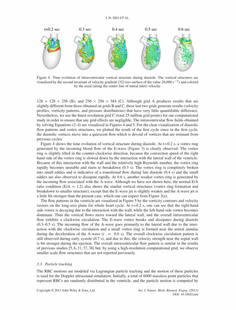
t=0.2 sec 0.3 sec 0.4 sec 0.5 sec 0.6 sec

Figure 4. Time evolution of intraventricular vortical structure during diastole. The vortical structures arevisualized by the second invariant of velocity gradient [32] (iso-surface of the value 20,000 s�2/ and colored

by the axial (along the center line of mitral inlet) velocity.

128 � 128 � 256 (B), and 256 � 256 � 384 (C). Although grid A produces results that areslightly different from those obtained on grids B and C, these last two grids generate results (velocityprofiles, vorticity patterns, and pressure distributions) that have very little quantifiable difference.Nevertheless, we use the finest resolution grid C (total 25 million grid points) for our computationalstudy in order to ensure that any grid effects are negligible. The intraventricular flow fields obtainedby solving Equations (2–4) are visualized in Figures 4 and 5. For the clear visualization of diastolicflow patterns and vortex structures, we plotted the result of the first cycle since in the first cycle,the diastolic vortices move into a quiescent flow which is devoid of vortices that are remnant fromprevious cycles.

Figure 4 shows the time evolution of vortical structure during diastole. At tD0.2 s, a vortex ringgenerated by the incoming blood flow of the E-wave (Figure 3) is clearly observed. The vortexring is slightly tilted in the counter-clockwise direction, because the convection speed of the righthand side of the vortex ring is slowed down by the interaction with the lateral wall of the ventricle.Because of this interaction with the wall and the relatively high Reynolds number, the vortex ringrapidly becomes unstable and starts to breakdown (0.3 s). The vortex ring is completely brokeninto small eddies and is indicative of a transitional flow during late diastole (0.4 s) and the smalleddies are also observed to dissipate rapidly. At 0.6 s, another weaker vortex ring is generated bythe incoming flow associated with the A-wave. Although we have not shown here, the normal E/Aratio condition (E/A D 1.2) also shows the similar vortical structures (vortex ring formation andbreakdown to smaller structure), except that the E-wave jet is slightly weaker and the A-wave jet isa little bit stronger than the present case, which one can expect from Figure 3(a).

The flow patterns in the ventricle are visualized in Figure 5 by the vorticity contours and velocityvectors on the long-axis plane for whole heart cycle. At tD0.2 s, one can see that the right-handside vortex is decaying due to the interaction with the wall, while the left-hand side vortex becomesdominant. Thus the vortical flows move toward the lateral wall, and the overall intraventricularflow exhibits a clockwise circulation. The E-wave vortex breaks and dissipates during diastole(0.3–0.5 s). The incoming flow of the A-wave goes primarily to the lateral wall due to the inter-action with the clockwise circulation and a small vortex ring is formed near the mitral annulasduring the deceleration of the A-wave (t D 0.6 s). The overall clockwise circulation pattern isstill observed during early systole (0.7 s), and due to this, the velocity strength near the septal wallis bit stronger during the ejection. The overall intraventricular flow pattern is similar to the resultsof previous studies [5, 6, 31, 37, 38] but, by using a high-resolution computational grid, we observesmaller scale flow structures that are not reported previously.

3.3. Particle tracking

The RBC motions are modeled via Lagrangian particle tracking and the motion of these particlesis used for the Doppler ultrasound simulation. Initially, a total of 6000 massless point particles thatrepresent RBCs are randomly distributed in the ventricle, and the particle motion is computed by



t=0.2 sec 0.3 sec 0.4 sec 0.5 sec

t=0.6 sec 0.7 sec 0.8 sec 0.9 sec

Figure 5. Vorticity contours and velocity vectors at the cross-section for whole heart cycle. Color contourdenotes y-component voriticy and the every eighth vectors are plotted.

t=0.1 sec 0.3 sec 0.5 sec 0.7 sec 0.9 sec

Figure 6. Distribution of RBCs computed by a Lagrangian particle tracking. Red: atrial RBCs, Blue:ventricular RBCs.

solving Equation (5). The particles are continuously injected though the mitral inlet during diastole,and the particles exiting the aorta during systole are removed. The RBC particle distributions duringthe cardiac cycle are shown in Figure 6. To examine the transport of RBCs, the particles that enterthrough the mitral inlet into the ventricle are tagged as ‘atrial’ RBCs (and colored red) and the RBC


J. H. SEO ET AL.

residing in the ventricle at the beginning of diastole are tagged as ‘ventricular’ RBC (and coloredblue). One can see the mixing of these two RBC groups by the ventricular vortices. The positionand velocity of each RBC particle are saved for the Doppler ultrasound computation described inthe next section. We note that the particle tracking can also be used for the analysis of ventricularwashout and blood residence time in the LV.

3.4. Doppler ultrasound simulation

For modeling the propagation of the ultrasound wave, we employed a transducer/receiver(transducer hereafter) of rectangular, parabolic shape. The size of the transducer is 2 � 1 cm(Figure 7(a)) and the distance to the focus point of the parabola is 3 cm. Note however that thecurrent approach allows us to use an ultrasound wave transducer of any shape. The main drivingfrequency (f / of ultrasound in our modeled transducer is 2 MHz, which is in the range of medi-cal ultrasound frequency. As shown in Equation (9), a higher driving frequency results in a largerfrequency shifting, thereby making it easier to detect small velocity changes. In the computer simu-lation, however, because there is virtually no lower limit to the detecting frequency shift, the choice

(a) (b)

(c)(d) t [sec]

V[m

/sec

]

0 0.2 0.4 0.6-0.5

0

0.5

1

1.5CFDVirtual Doppler

Figure 7. (a) Transducer position and the direction of ultrasound wave beam for the mitral inflow diagramand color M-mode. (b) Root-mean-squared velocity potential field for the current transducer. The coordinatesare centered at the center of transducer. (c) Simulated mitral inflow diagram. The thick red line indicates theactual mitral centerline velocity obtained from the flow field simulation result, and thin red lines are themaximum and minimum velocities in the sample volume of Doppler ultrasound obtained from the compu-tational fluid dynamics (CFD) result. (d) Comparison of temporal velocity profile at the mitral inlet; solidline: mitral centerline velocity from CFD, symbols: temporal profile of representative velocity based on the

maximum energy intensity on the spectrogram of virtual Doppler simulation.



of driving frequency does not play an important role. The more important parameter in the Dopplerultrasound simulation is the sampling frequency,(f /k,where k is an integer) because the samplingfrequency limits the range of detected velocity which is given by jvj 6 c/(4k/. Here, we use kranging from 100 to 200 and the maximum range of detected velocity is˙3.75 (m/s) which is largeenough to resolve intraventricular flow velocity.

A key feature of the ultrasound transducer model is the discretization of the transducer surface.In the current simulations, it is discretized by 160 triangular elements for the computation and eachelement acts as a point source of ultrasonic energy. If the number of surface elements (number ofpoint sources) is too small, the resulting ultrasound field becomes irregular and nonuniform, whiletoo many elements significantly increase the computational time because the computational costis proportional to the square of the number of elements. The present number of surface elementsprovides a smooth ultrasound field with reasonable computational time. For example, the com-putation of M-mode Doppler with 40 volume samples takes about 12 hours using 40 CPUs. Theroot mean squared velocity potential of sound wave emitted by the current transducer computed byEquation (6) is plotted in Figure 7(b). With the present setup, the distance from the transducer to thefocal point (the point of maximum intensity) is about 6 cm, and the ventricle is placed at the focaland far-field region. The Doppler ultrasound simulations are performed by Equations (8) and (10)using the RBC particle motions shown above.

The model of ultrasound is first used in a pulsed Doppler mode to extract the mitral inflow veloc-ity from our CFD model. The mitral inflow diagram shows the temporal velocity profile throughthe mitral inlet and is used to determine the clinically important parameters such as the E/A ratioand the E-wave deceleration time [8]. In the current computational study, the transducer is locatedat the center of mitral inlet and 11 cm below from the mitral valve location. The ultrasound wavebeam is perfectly aligned with the mitral inlet axis (z-dir). The pulse duration is 1 �s and the pulserepeating frequency is 10 kHz. The target sample volume is at a distance of 11 cm from the trans-ducer (i.e., mitral valve location). The mitral inflow diagram is obtained from the spectrogram ofthe received signal (Equation 11) and plotted in Figure 7(c). In this figure, the thick red line indi-cates the actual velocity at the mitral center line obtained directly from the flow simulation andthin red lines are the minimum and maximum velocities in the sample volume of Doppler ultra-sound. Grayscale contours represent the normalized energy intensity, S(t,V)/Smax(t) of the scatteredultrasound wave signal received by the transducer. Here Smax(t) is the maximum energy intensityat the given time instance. Thus the diagram shows the distributions of the velocity detected by theDoppler ultrasound and the velocity value corresponding to the maximum energy intensity, Smax canbe considered as the representative velocity of the sample volume.

We note that the temporal variation of the mitral inflow velocity evaluated by the Doppler ultra-sound agrees well with the actual velocity profile. Because the ultrasound scans the volume of bloodflow instead of a point and the blood flow velocities in that volume are not constant, the velocityobtained by the Doppler ultrasound is slightly dispersed around the actual velocity at a point butit is bounded well by the actual maximum and minimum velocities in the sample volume, exceptaround the peak of E-wave. The overestimated dispersion of velocity value at around the E-wavepeak may be caused by the signal processing. Specifically, for higher velocity (i.e., higher �f /,the number of time sampling point per wavelength decreases, and this will cause the energy disper-sion but it can be resolved by increasing the sampling rate. We note however that the representativevelocity profile conforms very well with the centerline velocity profile from the CFD as shown inFigure 7(d) and this verifies the present velocity measurement procedure using the Doppler ultra-sound simulation. Although we imposed an E/A ratio of 2 based on the volume averaged peakvelocity for the E and A waves, the E/A ratio evaluated from Figure 7(c) based on the velocityvalue of maximum energy intensity at the peaks of E and A waves is 0.918(m/s)/0.406(m/s)D2.26.This suggests the potential of the current virtual ECHO model to help identify possible sourcesof error in Doppler based velocity measurements. Because we already know the exact velocityvalue and the current Doppler ultrasound modeling excludes all the sources of uncertain errors (e.g.external noise, effects of tissue Doppler, and etc.), the present ECHO model can be used to inves-tigate the effects of signal processing, duty-cycle and sampling frequencies, and transducer typeand geometry.


J. H. SEO ET AL.

The assessment of mitral inflow velocity using the virtual ECHO will also help the validation andcalibration of a patient specific heart model for cardiac flow simulations. Because the mitral inflowis in fact the inflow boundary condition, the ventricular flow pattern will be very sensitive to themitral inflow profile. If one perform the virtual ECHO using the same transducer type, driving andsampling frequencies, and ultrasound wave beam direction with the actual ECHO, the virtual ECHOdata can directly be compared to the actual one, and based on that, one can validate or calibrate thepatient specific computational heart model. For example, if the magnitude of inflow velocity is notmatched, it means that the volume change rate of the LV model is incorrect. This would not be arare situation especially if the patient-specific heart model would be based on functional (4D) CTscans which typically do not have a high temporal sampling rate (e.g. 12 frames for a cycle). Thus,the ECHO data based calibration will improve the reliability of patient specific heart models.

Next, the virtual ECHO is used in the color M-mode to produce diastolic wave velocity patterns.The transducer position and properties of PW ultrasound are the same with the above case, and thevelocity field of the second cardiac cycle (16t62 (s)) is used. The velocities for a total of 40 samplevolumes are extracted from the apex to the mitral annulus and the spatial resolution of sampling is2 mm. The resulting color M-mode image is shown in Figure 8(a). Here a positive velocity indicatesflow toward the transducer, that is, from the mitral to the apex. Figure 8(b) shows the similar plotmade by using the ´-direction velocity values directly obtained from the flow field computation andit shows very good correlation with the simulated color M-mode Doppler plot. This comparisonalso proves that the direct velocity data from CFD can be used as the surrogate of color M-modediagram [6, 31]. Note that, however, the direct CFD data cannot incorporate the effects of ultra-sound and transducer parameters. In Figure 8(a), one can see the propagation of blood flow whichcomes into the ventricle with the E and A waves. The propagation velocity of blood flow, vp, isusually evaluated by the slope of the velocity contour (based on the contour at 50% of the maximumvelocity [7]) on the color M-mode image and used as a parameter to estimate the ventricle function[14]. In the present case, the propagation velocity for the E-wave is estimated to be about 31 cm/s(black solid line in Figure 8(a)) which is in the range (37˙12 cm/s) reported by Garcia et al. [7] forhuman study with 14 elderly patients (age: 64˙11). It has been reported that vp is about 70 cm/sfor the normal ventricle with physiological E/A ratio but it decreases to about 24 cm/s for low orhigh E/A ratios [14]. Another index suggested for the assessment of ventricular function is vE/vp,where vE is the peak velocity of E-wave, and vE/vp >1.5 for the diseased ventricles [14]. For thepresent case, the conditions correspond to severe diastolic dysfunction with E/AD2 and vE/vp yields2.96. However, a proper way to determine the propagation velocity, vp, is still arguable [39]. Withthe current computational hemodynamics and Doppler ultrasound simulation approach, it is pos-sible to investigate the correlation between the evaluated propagation velocity based on the colorM-mode and the actual blood transportation velocity, and also the correlation between the

Figure 8. Temporal velocity variation along the mitral center line. (a) Simulated color M-mode Dopplerimage obtained from our Doppler model. The positive velocity value indicates the flow direction from themitral to the apex. The slope of black line represents the flow propagation velocity for the E-waves. Theestimated propagation velocity is about 31 cm/s. (b) Mitral center line velocity data obtained directly from

the flow simulation.



Figure 9. (a) Transducer position and the direction of ultrasound wave beam for continuous wave Doppler.(b) Simulated continuous wave Doppler diagram for the left ventricle outflow tract. (c) Instantaneous gaugepressure contours at t D 0.8 s on the plane tangent to the direction of ultrasound wave beam. Point A is the

location of maximum blood flow velocity.

ventricular hemodynamics (e.g. LV axial pressure gradient) and vp or vE/vp. These will be pursuedin a future study.

Finally, we demonstrate the generation of a CW Doppler image using our modeling procedure.This mode of ultrasound operation is particularly useful when the primary interest is determin-ing extreme values of velocity in the path of the beam. Clinical applications include determiningflow velocity in peripheral arteries and estimation of blood flow and pressure in the left ventricu-lar outflow tract and aorta [9]. For this demonstration we focus on the left ventricle outflow tract(LVOT) which is particularly relevant to pathologies such as obstructive hypertrophic cardiomy-opathy (HOCM). For this condition, CW Doppler is used to find the maximum blood flow velocityin the LVOT. Once the maximum velocity is obtained, the LVOT pressure gradient is evaluatedby a simplified Bernoulli equation; �P ŒmmHg D 4.V Œm/s/2. The LVOT pressure gradient is animportant factor in diagnosing the significance of aortic stenosis or HOCM in the LVOT.

In our model, the transducer of the same shape as described earlier is placed on the locationshown in Figure 9(a) and the direction of ultrasound beam is aligned with the blood flow directionin LVOT. The CW Doppler image is obtained from the spectrogram of the received signal and plot-ted in Figure 9(b). Because the CW scans all the blood volume that lies in the path of the ultrasoundbeam, the Doppler signal detects an entire range of velocity values at any given time-instance. Inour model, the negative peak around 0.8 s (see Figure 9(b)) is the maximum blood flow velocitythrough the LVOT during the ejection and the value is about 2.1 m/s. The maximum LVOT pres-sure gradient estimated by the simplified Bernoulli equation is 17.6 mmHg. Figure 9(c) shows theinstantaneous pressure field on the plane tangent to the direction of ultrasound wave beam obtainedby the computational hemodynamic simulation. Point A is the location of the maximum blood flowvelocity and the maximum velocity value is 2.18 m/s which is very close to the value obtained bythe CW Doppler. The pressure difference computed directly in the flow simulation between pointA and point B (i.e., LVOT pressure gradient) is however about 15 mmHg. Thus the LVOT pressuregradient is slightly over predicted by 4V 2, a tendency that has also been reported from the in-vivoassessments of this technique [9]. Note however that while the pressure inside the LV is almostspatially uniform, the pressure in the aorta varies noticeably based on location. Thus, the presentcomputational hemodynamics and Doppler ultrasound simulation approach can perform a criticalassessment of the LVOT pressure gradient estimation. This will be pursued for the sub-aortic LVOTobstruction in the further study.

3.5. Simulation of systolic ejection murmur

Heart sound contains important information regarding the health of the cardiac system and auscul-tation has been used as a noninvasive diagnostic modality for heart disease for many thousands of


J. H. SEO ET AL.

years. In PC, heart sounds are recorded using an electronic-stethoscope and the resultingphonocardiogram is analyzed in order to detect abnormal heart sounds associated with heart dis-ease [11]. However, the correlation between heart disease, flow patterns and heart sounds is still notfully understood. This is primarily due to the fact that there exist no measurement techniques thatcan measure ventricular flow patterns and the corresponding heart sounds simultaneously. Thus, acomputational technique that can enable the generation of such correlations could have a signifi-cant impact on the clinical technique of PC. The application of such correlations run the gamut ofheart disease including but not limited to innocent/functional murmurs in children [40], sounds ofdiastolic dysfunction [13], and systolic murmurs [10] associated with mitral regurgitation aortic andLVOT obstruction.

In the current study, we predict the generation of abnormal heart sound through direct computa-tion of flow and sound and use this to generate a virtual phonocardiogram. In particular, we considerhere a systolic ejection murmur caused by a hypertrophic (obstructive) cardiomyopathy (HOCM). Itis generally believed that the systolic ejection murmur is generated by the blood flow disturbancesdue to an obstruction in left-ventricular outflow tract (LVOT) [10] and, in the present study wecompute directly the generation and propagation of the murmurs associated with HOCM.

A simplified two-dimensional model of the LV with the ascending aorta is constructed to simu-late the flow and associated murmurs during systole (Figure 10(a)). Here, DA D 2 cm, dT D 7 cm,DLV D 6.4 cm, and LLV D 7.4 cm (at the beginning of systole). A sub-aortic, obstructive hyper-trophy is modeled as shown in Figure 10 for the HCM cases. In addition to a normal case, weconsidered two HCM cases, HCM1 and HCM2, and HCM2 has more severe obstruction thanHCM1. For the HCM cases, the mitral valve leaflets are elongated and migrated toward the out-flow tract to mimic systolic anterior motion (SAM) which manifests in many severe cases of HCM[41]. In reality, the elongated mitral leaflet can fluctuate along with the flow instability and it maygenerate additional sound associated with flow-structure interaction. In the present study, however,such a dynamic motion of the leaflets is not considered, and we focus on the flow noise sourcecaused by the obstruction. It is also assumed that the two HCM cases have the same degree of SAM.The resulting gap size in the outflow tract is about 0.3DA for HCM1 and 0.2DA for HCM2. Thesimulations are performed for only the systolic phase of the cardiac cycle. The temporal blood flowrate profile is given in Equation (14), but the systolic period (tES -tSS / of 0.25 s is used here. Theblood flow domain inside the LV and aorta (indicated by shaded area in Figure 10) is resolved by256� 384 nonuniform Cartesian grid (see Figure 10(b)) with the minimum grid spacing of 0.015DA.The flow simulation is performed by solving Equations (1-4).

Figure 10. (a) Schematic diagram of simplified left ventricle model with hypertrophy for the computationof systolic ejection murmur. The shaded area (for HCM2 case) indicates the flow domain and H D 1 regionfor Equation (13), whereas H D 0 for white area. (b) Computational domains and grids for the flow and

acoustic simulations. Every fourth grids are plotted for the clarity.



The sound generation by the blood flow and its propagation in blood and tissue regions areresolved by the acoustic equations, Equation (13). Thus the acoustic domain includes the LV andaorta as well as nearby thoracic region represented by the box in Figure 10(a). The acoustic compu-tation is performed on a separate grid which consists of 200�200 grid points (see Figure 10(b)) witha minimum grid spacing of 0.04DA. The flow simulation results are interpolated onto the acousticgrid in the LV and aorta region using a bi-linear interpolation. The density and speed of sound forthe blood are set to 1.05 (g/cm3/ and 1500 (m/s), respectively. For the present simplified thoraxmodel, a thoracic region outside the heart is assumed to consist of a homogeneous tissue materialand its density and speed of sound are assumed to be 1.2 (g/cm3/ and 1800 (m/s). These values areaveraged material properties of various components in the thorax [42]. The density and speed ofsound (i.e., the bulk modulus, K D �c2/ scales with the amplitude of acoustic pressure fluctuation(p0 � K/ and the wavelength ( D f /c, where f is the frequency) in an open space. In the PC,the waveform of acoustic signal is primarily used to identify the types of murmur [10]. For a typicalfrequency range of a murmur (�O(100) Hz), the wavelength is much longer than any length scalesin the thorax for c >100 (m/s), and thus the waveform of murmur is not so sensitive to the slightchange in the bulk modulus. The left boundary of the acoustic domain represents the precordiumsurface and the heart sound is monitored there as is done in actual auscultation. Because a stetho-scope senses transmitted sound via the velocity (or acceleration) of the precordium surface [43], wehave recorded the velocity fluctuations on the monitoring points shown in Figure 10(a). The zero-stress boundary condition is applied at the precordium surface and it is assumed that acoustic wavesradiate through all other boundaries.

The instantaneous hemodynamic flow fields for normal, HCM1, and HCM2 cases are shown inFigure 11 with the vorticity contours. For the normal case, there is no significant vortex motion inthe LVOT and aorta. With HCM and SAM, however, the formation of a jet in the gap between thehypertrophy and the mitral valve leaflet is observed and the jet shear layer rolls into vortices whichinteract with the aortic wall. This complex vortex motion is supposed to be the source of murmursound. For the smaller gap (HCM2), the blood flow velocity through the gap is faster and exhibitsstronger vortex motions.

The acoustic fields are computed by Equation (13) using the computed flow field and pressure.Figure 12 shows the root-mean-squared acoustic fields for the HCM2 case. Interestingly, it seemsthat the dominant sound originates from the ventricle region rather than the aorta. The velocity fluc-tuations monitored on the precordium surface are plotted in Figure 13(a) for HCM1 and HCM2cases. For normal case, no significant velocity fluctuation is observed. Figure 13(a) is the recordedmurmur signal for the cases with HCM and can be considered as a virtual phonocardiogram forthe HCM murmur. The present simulated murmur signal exhibits an ascendo/descendo configura-tion [10] (especially for HCM2) which is quite common in systolic murmurs. Note that, with larger

Normal HCM1 HCM2

Figure 11. Instantaneous hemodynamic flow field for the normal and hypertrophic cardiomyopathy (HCM)cases represented by vorticity contours at t D 0.13 s (t D 0 is the start of systole phase).


J. H. SEO ET AL.

Figure 12. Acoustic fields of hypertrophic cardiomyopathy (HCM) systolic murmur for HCM2 case.Root-mean-squared acoustic pressure fluctuation (left) and x-direction velocity fluctuation (right) contours.

Here, Vmax is the peak averaged blood flow velocity in the aorta exit during the systole.

Figure 13. (a) Acoustic velocity fluctuation monitored on the precordium surface. Time signal band-passfiltered for 20–400 Hz. (b) Time-frequency spectrogram. (c) Evaluated source term; volume integratedhydrodynamic pressure fluctuation, Sa D

R.DP=Dt/dV LV: integration over the LV region, AO:

integration over the aorta region.

hypertrophy (HCM2), a stronger murmur is generated. Figure 13(b) shows the time-frequency spec-trograms of the murmur signals. The strongest energy is found at 64 Hz for HCM1 and 110 Hz forHCM2. HCM2 case also has higher frequency components. Thus in the present results the moresevere HCM produces stronger and higher frequency murmur sound.



Figure 14. Propagation of systolic HCM murmur computed with a realistic human thorax model. (a) and(b) Root-mean-squared acoustic pressure and velocity fluctuations plotted on the density iso-surfaces. (c)Phonocardiac signals for the hypertrophic cardiomyopathy (HCM) systolic murmur monitored on points Aand B in Figure 14(b). The signals are band-pass filtered for 20–400 Hz. Here, � and c are the density and

the speed of sound of the blood.

Based on the acoustic equation (Equation 13), we have found that the murmur is in fact correlatedwith the volume integrated hydrodynamics pressure fluctuation. Thus we define the source term;Sa.t/ D

R.DP=Dt/.Ex, t /dV , and it is plotted in Figure 13(c). In order to identify the primary

source region of the murmur, we evaluated Sa for the LV and aorta regions separately. One can seethat the time signal of Sa is correlated very well with the murmur signal, and the primary contri-bution to this source term comes from the LV region rather than the aorta, which is inline with theresult shown in Figure 12.

Now in order to examine the effect of heart sound propagation in a real human thorax whichincludes many different biological materials such as chest bones and lungs, we have considereda three-dimensional realistic human thorax model. The model is constructed based on the VisibleHuman®‡ Dataset. For the simulation of sound propagation, the contrast value on the CT scanimages is converted to the material density and speed of sound using the formulation proposed inRef. [29]. The density varies from 0.1 g/cm3 to 2.0 g/cm3, and we truncated the values that areout of this range. The speed of sound varies from 292 m/s to 2914 m/s. These three-dimensionaldensity and speed of sound fields are mapped on the Cartesian grid of 140�160�80 grid pointswith the grid spacing of 2.175 mm. Equation (13) is solved with H=0, but the source term, DP/Dton the right hand side is kept. For the sound source, we use DP/Dt value on the LV obtainedfrom the hemodynamic flow field simulation of HCM2 case.We first calculate the volume aver-age of DP/Dt over the ventricle, .DP=Dt/ .t/ D

R.DP=Dt/.Ex, t /dV=

RdV and this source term

is placed inside the thorax model at a location typical for the LV as a distributed point source:.DP=Dt/LV .Ex, t / D .DP=Dt/ .t/ � exp.�

ˇ̌Ex � ExLV

ˇ̌2=r2w/, where ExLV is the position vector to

the center of LV on the thorax model and rw D 1 cm. Figure 14(a) and (b) show the root-mean-squared acoustic fields of HCM murmur radiated in the realistic thorax model. One can clearly see

‡An anatomical data set developed under a contract from the National Library of Medicine by the Departments of Cellularand Structural Biology, and Radiology, University of Colorado School of Medicine


J. H. SEO ET AL.

the high pressure fluctuation around the heart location and high velocity fluctuation on the chest sur-face above the heart. The velocity fluctuations are monitored on the two locations A and B shown inFigure 14(b) and plotted in Figure 14(c). Figure 14(c) is thus the virtual phonocardiogram of HCMmurmur predicted with the realistic thorax model. The point A is on the chest surface directly abovethe heart, thus the signal monitored at this point shows higher amplitude than point B. Interestingly,the signal monitored at point A looks very similar with the result of simplified thorax model shownin Figure 13(a)(HCM2). This implies that the effect of sound propagation in heterogeneous mediumis not so significant for the present low frequency signal (�O(100) Hz). This observation agreeswith the result of Narasimhan et al. [29].

The present coupled computational hemodynamic-hemoacoustic approach for the virtual phono-cardiogram can be used for a comprehensive investigation of the heart sound generation mechanismand it has the potential to improve the diagnostic ability of the cardiac auscultation. The presentmethod will also be applied to the third and fourth heart sounds [13] to reveal the generationmechanism of those abnormal heart sounds.

4. CONCLUSION

In the current study, methods for the modeling and simulation of intraventricular blood flows,Doppler ultrasound, and blood flow induced heart sound are presented. Blood flow is modeled usinga high-fidelity, immersed boundary based Navier–Stokes solver. Virtual ECHO and PC signals areconstructed from results of computational hemodynamic simulations by modeling the physics ofDoppler ultrasound and heart sound, respectively. The reconstruction of mitral inflow diagram, colorM-mode Doppler, and CW Doppler in the left-ventricular outflow tract, and the simulation of sys-tolic HCM murmur are demonstrated, and the possible applications of these virtual cardiographiesare also discussed. These virtual cardiographic data not only provide new ways to interpret compu-tational hemodynamic results but also allows us to investigate the correlation between the diagnosticdata and specific features of the hemodynamic flow patterns. The development of comprehensivecorrelations between blood flow dynamic and cardiographic output parameters obtained from thecurrent multi-phyiscs modeling approach is expected to provide new insights into the diagnosis andassessment of a variety of heart conditions.

ACKNOWLEDGEMENTS

This research is supported by the CDI program at NSF through grant IOS-1124804. This work used theExtreme Science and Engineering Discovery Environment (XSEDE), which is supported by NSF grantnumber TG-CTS100002. The Visible Human® Dataset was provided by the National Library of Medicine.The authors also thank Dr. Albert C. Lardo for providing the contrast CT scan data of the LV

REFERENCES

1. Domenichini F, Pedrizzetti G, Baccani B. Three-dimensional filling flow into a model left ventricle. Journal of FluidMechanics 2005; 539:179–198.

2. Mihalef V, Ionasec R, Sharma P, Georgescu B, Voigt I, Suehling M, Comaniciu D. Patient-specifc modelling ofwhole heart anatomy, dynamics and hemodynamics from four-dimensional cardiac CT images. Journal of the RoyalSociety Interface Focus 2011; 1:286–296.

3. Saber NR, Gosman AD, Wood NB, Kilner PJ, Charrier CL, Firmin DN. Computational Flow modeling of the leftventricle based on in vivo MRI data: Initial experience. Annals of Biomedical Engineering 2001; 29:275–283.

4. Saber NR, Wood NB, Gosman AD, Merrifield RD, Yang G, Charrier CL, Gatahouse PD, Firmin DN. Progess towardspatient speci?c computational flow modeling of the left heart via combination of magnetic resonance imaging withcomputational fluid dynamics. Annals of Biomedical Engineering 2003; 31:42–52.

5. Schenkel T, Malve M, Markl M, Jung B, Oertel H. MRI-based CFD analysis of flow in a human left ventriclemethodology and application to a healthy heart. Annals of Biomedical Engineering 2009; 37(3):505–515.

6. Watanabe H, Sugiura S, Kafuku H, Hisada T. Multiphysics simulation of left ventricular filling dynamics usingfluid-structur interaction finite element method. Biophysical Journal 2004; 87:2074–2085.

7. Garcia JM, Smedira NG, Greenberg NL, Main M, Firstenberg MS, Odabashian J, Thomas JD. Color M-modeDoppler flow propagation velocity is a preload insensitive index of left ventricular relaxation: animal and humanvalidation. Journal of the American College of Cardiology 2000; 35:201–208.



8. Nishimura RA, Tajik A. Evaluation of diastolic filling of left ventricle in health and disease: Doppler Echocardiog-raphy is the Clinician’s Rosetta Stone. Journal of the American College of Cardiology 1997; 30:8–18.

9. Sasson Z, Yock PG, Hatle LK, Alderman EL, Popp RL. Doppler echocardiographic determination of the pressuregradient in hypertrophic cardiomyopathy. Journal of the American College of Cardiology 1988; 11:752–756.

10. Alpert MA. Systolic murmurs. In Clinical Methods: The History, Physical, and Laboratory Examinations, WalkerHK, Hall WD, Hurst JW (eds), Chapter 2, 3rd Ed. Boston: Butterworths, 1990.

11. Erne P. Beyond auscultation - Acoustic cardiography in the diagnosis and assessment of cardiac disease. SwissMedical Weekly 2008; 138:439–452.

12. Murgo JP. Systolic ejection murmur in era of modern cardiology, what we really know? Journal of the AmericanCollege of Cardiology 1998; 32(6):1596–1602.

13. Ronan JA, Jr. Cardiac auscultation: the third and fourth heart sounds. Heart Disease and Storke 1992; 1(5):267–270.14. Boeck BWL, Oh JK, Vandervoort PM, Vierendeels JA, Aa RPLM, Cramer MJM. Color M-mode velocity propa-

gation: a glance at intra-ventricular pressure gradients and early diastolic ventricular performance. The EuropeanJournal of Heart Failure 2005; 7:19–28.

15. Mittal R, Dong H, Bozkurttas M, Najjar FM, Vargas A, von Loebbecke AA. A versatile sharp interface immersedboundary method for incompressible flows with complex boundaries. Journal of Computational Physics 2008;227:4825–4852.

16. Oung H, Forsberg F. Doppler ultrasound simulation model for pulsatile flow with non-axial components. UltrasonicImaging 1996; 18:157–172.

17. Seo JH, Moon YJ. Linearized perturbed compressible equations for low Mach number aeroacoustics. Journal ofComputational Physics 2006; 218:702–719.

18. Chorin AJ. On the convergence of discrete approximations to the Navier–Stokes equations. Mathematics ofComputation 1969; 23(106):341–353.

19. Bozkurttas M, Dong H, Seshadri V, Mittal R, Najjar F. Towards numerical simulation of flapping foils on fixedCartesian grids. 43th AIAA Aerospace Sciences Meeting and Exhibition, Jan. 10-13, AIAA Paper 2005-0081, Reno,Nevada, 2005.

20. McQueen DM, Peskin CS. Heart Simulation by An Immersed Boundary Method with Formal Second-Order Accuracyand Reduced Numerical Viscosity, Mechanics for a New Mellennium. Kluwer Academic Publisher: New York, 2002;pp. 429-444.

21. Peskin CS, McQueen DM. A three-dimensional computational method for blood flow in the heart I. Immersed elasticfibers in a viscous incompressible fluids. Journal of Computational Physics 1989; 81(2):372–405.

22. Jensen JA, Svendsen NB. Calculation of pressure fields from arbitrarily shaped, apodized, and excited ultrasoundtransducers. IEEE Transactions on Ultrasonics, Ferroelectrics and Frequency Control 1992; 30:262–267.

23. Tan L, Jiang J. Fundamental of: Analog and Digital Signal Processing. AuthorHouse: Bloomington, Indiana, USA,2007; pp. 279.

24. Moon YJ, Seo JH, Bae YM, Roger M, Becker S. A hybrid prediction method for low-subsonic turbulent flow noise.Computers & Fluids 2010; 39:1125–1135.

25. Seo JH, Mittal R. A high-order immersed boundary method for acoustic wave scattering and low Mach number flowinduced sound in complex geometries. Journal of Computational Physics 2011; 230:1000–1019.

26. Seo JH, Mittal R. A coupled flow-acoustic computational study of bruits from a modeled stenosed artery. Medical &Biological Engineering & Computing 2012; 50:1025–1035.

27. Okita K, Ono K, Takagi S, Matsumoto Y. Development of high intensity focused ultrasound simulator for large-scalecomputing. International Journal for Numerical Methods in Fluids 2010; 65:43–66.

28. Baron C, Aubry JF, Tanter M, Meairs S, Fink M. Simulation of intracranial acoustic fields in clinical trialssonothrombolysis. Ultrasound in Medicine & Biology 2009; 35(7):1148–1158.

29. Narasimhan C, Ward R, Kruse KL, Gudatti M, Mahinthakumar G. A high resolution computer model for soundpropagation in the human thorax based on the Visible Human data set. Computers in Biology & Medicine 2004;34:177–192.

30. Lele SK. Compact finite difference schemes with spectral-like resolution. Journal of Computational Physics 1992;103:16–42.

31. Zheng X, Seo JH, Vedula V, Abraham T, Mittal R. Computational modeling and analysis of intracardiac flows insimple models of the left ventricle. European Journal of Mechanics - B/Fluids 2012; 35:31–39.

32. Jeong J, Hussain F. On the identification of a vortex. Journal of Fluid Mechanics 1995; 285:69–94.33. Domenichini F, Querzoli G, Genedese AG, Pedrizzetti G. Combined experimental and numerical analysis of the flow

structure into the left ventricle. Journal of Biomechanics 2007; 40:1988–1994.34. Redfield MM, Jacobsen SJ, Burnett JC, Jr., Mahoney DW, Bailey KR, Rodeheffer RJ. Burden of systolic and dias-

tolic ventricular dysfunction in the community; Appreciating the scope of the heart failure epidemic. The Journal ofthe American Medical Association 2003; 289(2):194–202.

35. Taylor TW, Suga H, Goto Y, Okino H, Yamaguchi T. The effects of cardiac infarction on realistic three-dimensionalleft ventricular blood ejection. Transactions of the ASME Journal of Biomechanical Engineering 1996; 118:106–110.

36. Moghadam ME, Bazilevs Y, Hsia TY, Vignon-Clementel IE, Marsden AL. A comparison of outlet boundary treat-ments for prevention of backflow divergence with relevence to blood flow simulations. Computational Mechanics2011; 48:277–291.


J. H. SEO ET AL.

37. Doenst T, Spiegel K, Reik M, Markl M, Henning J, Nitzsche S, Beyersdorf F, Oertel H. Fluid-dynamics modeling ofthe human left ventricle: methodology and application to surgical ventricular reconstruction. The Annals of ThoracicSurgery 2009; 87:1187–1195.

38. Kilner PJ, Yang G, Wilkes AJ, Mohiaddin RH, Firmin N, Ycoub MH. Asymmetric redirection of flow through theheart. Nature Letter 2000; 404:759–761.

39. Casandra N, Takahiro O, Pavlos V, William L. Measuring heart filling propagation velocity using the cross wavelettransform. 64th Annual Meeting of the APS Division of Fluid Dynamics, November 20-22, 2011; abstract #D13.002.

40. Smith KM. The innocent heart murmur in children. Journal of Pediatric Health Care 1997; 11:207–214.41. Levine RA, Vlahakes GJ, Lefebvre X, Guerrero JL, Cape EG, Yoganathan AP, Weyman AE. Papillary muscle

displacement causes systolic anterior motion of the mitral valve, Experimental validation and insights into themechanism of subaortic obstruction. Circulation 1995; 91:1189–1195.

42. Goss SA, Frizzell LA. Dunn F Dependence of the ultrasonic properties of biological tissue on constituent proteins.Journal of the Acoustical Society of America 1980; 67(3):1041–1044.

43. Borisyuk AO. Noise field in the human chest due to turbulent flow in large blood vessel. Flow, Turbulence andCombustion 1999; 61:269–284.


multiphysics computational models for cardiac flow - mechanical

Documents