multiple approaches to solve tank scheduling problems
TRANSCRIPT

Multiple approaches to solve tank scheduling problems
Name: R.P.J. BrochStudent number: 289584Date: July 2010
University supervisor: Dr. Wilco van den Heuvel
Erasmus University RotterdamEconometrics & Management ScienceMaster Operations Research & Quantitative Logistics

1
AbstractIn this thesis the tank scheduling problem is investigated. In this problem intermediate storage tanks are used to decouple production stages of juices, soda, etc. so that they are less dependent on each other. The tanks will have to store intermediate products and that is where the tank scheduling problem starts. Scheduling of tanks by hand is too complex, that is why algorithms or mathematical programming approaches should be used. Genetic algorithms, greedy algorithm, mixed integer linear programming and constraint programming are the techniques implemented and used for computational tests. The latter three provide good results in terms of solving time and quality of the tank schedules. On the other hand genetic algorithms do not provide satisfying results.Different variants of tank scheduling problems appear to have different solving approaches which suit them best.

2
Table of contentsAbstract ................................................................................................................................................... 1Table of contents..................................................................................................................................... 21 Introduction................................................................................................................................... 42 Literature ....................................................................................................................................... 63 Problem description ...................................................................................................................... 8
3.1 General layout........................................................................................................................ 83.2 Physical constraints................................................................................................................ 83.3 Overall assumptions............................................................................................................... 93.4 Specific problems................................................................................................................. 103.5 Extensions ............................................................................................................................ 113.6 Data...................................................................................................................................... 113.7 Assignment problem............................................................................................................ 13
4 Genetic algorithm approach........................................................................................................ 154.1 Some definitions .................................................................................................................. 154.2 Genetic algorithm Operators ............................................................................................... 15
4.2.1 Selection ............................................................................................................................ 154.2.2 Crossover ........................................................................................................................... 164.2.3 Mutation ............................................................................................................................ 184.2.4 Elitism................................................................................................................................. 184.2.5 Procedure basic GA............................................................................................................ 18
4.3 Implementation genetic algorithm...................................................................................... 184.3.1 Step 1 - Encode solutions................................................................................................... 184.3.2 Step 2 - Set population size n............................................................................................. 194.3.3 Step 3 - Initialization population........................................................................................ 204.3.4 Step 4 - Fitness evaluation................................................................................................. 204.3.5 Step 5 - Elitism ................................................................................................................... 204.3.6 Step 6 - Reproduction ........................................................................................................ 204.3.7 Step 7 - Stopping criterion ................................................................................................. 20
4.4 GAvAPS................................................................................................................................. 204.4.1 Introduction ....................................................................................................................... 204.4.2 Outline GAVaPS.................................................................................................................. 21
4.5 Greedy Algorithm................................................................................................................. 214.6 Results.................................................................................................................................. 23
4.6.1 Genetic algorithm .............................................................................................................. 234.6.2 GAVaPS .............................................................................................................................. 244.6.3 Greedy algorithm............................................................................................................... 264.6.4 Overview results ................................................................................................................ 26
4.7 Shift production ................................................................................................................... 275 MIP approach .............................................................................................................................. 29
5.1 Relaxing fixed production dates - Model 1 .......................................................................... 295.2 Relaxing fixed production dates - Model 2 .......................................................................... 325.3 Relaxing fixed consumption dates ....................................................................................... 355.4 Results.................................................................................................................................. 39
6 Constraint programming approach ............................................................................................. 426.1 An introduction .................................................................................................................... 42

3
6.2 Implementation constraint programming ........................................................................... 456.2.1 Basic models ...................................................................................................................... 456.2.2 Extended model................................................................................................................. 48
6.3 Results.................................................................................................................................. 507 Conclusions and recommendations ............................................................................................ 53References............................................................................................................................................. 55

4
1 IntroductionIn this section the main topic of this master thesis is presented. First the problem is introduced and explained briefly. Next the goal of this thesis and its outline are given.
Production processes are usually made up of multiple stages. Liquids like dairy products and sodas for example undergo pasteurization, mixing and/or bottling. All these processes depend on each other. When something goes wrong in one process this could lead to other processes being interrupted. Intermediate storage tanks are used to decouple the different processes such thatproductions and production stages are less dependent on each other. Now not only finished products need to be stored but also semi-finished products. When a semi-finished product is stored in a tank,it will wait for the next part of the production process. A consequence of decoupling the stages is that it increases efficiency of production so that more productions can be carried out. An example of efficiency increase is that if a production machine is able to fill a tank at a faster rate than the rate that they can be emptied by another machine, then filling does not need to adjust its rate to the rate of emptying.
As a result of the use of intermediate storage tanks, product flows occur between machines and tanks and vice versa. This requires the need for tank scheduling; the creation of a timetable in which product flows, from machines to storage tanks and from storage tanks to machines, are assigned respecting the existing restrictions. It can be a serious planning task due to some typical scheduling issues. For example, is it allowed to store multiple product flows in one tank and to store a product in multiple tanks or not? These and other issues/restrictions will be explained in chapter 3.
The goal of this master thesis is to solve tank scheduling problems with the use of different techniques and to compare the results and the limitations of each technique. The three explored approaches are genetic algorithm (GA), mixed integer programming (MIP) and constraint programming (CP). It will be shown that different variants of tank scheduling problems favor different techniques. An advantage of GA’s is that the objective function and constraints can be designed the way you want and implemented with ease. A disadvantage with GA’s is that you do not always know if a solution is optimal or not. This is true when, for example, the objective function is equal to the makespan of the tank schedule. This does not pose a problem when the objective is just to find a feasible schedule. With MIP the advantages are that optimality can be proven and that problems are stated infeasible when infeasibilities exist. On the other hand, in MIP constraints and objective function need to be linear such that the construction of adequate formulations is not self-evident. CP is a very flexible method and easy to implement and also has the advantages of the other two methods just mentioned. Disadvantages are the requirement of integer decisions variables and the one-sided bound (instead of two-sided) on objective functions making it difficult to state optimality when optimal. Summarized, every technique has its pros and cons and implementation of the techniques will show which technique suits the tank scheduling problem best.
The outline of this thesis is as follows. Chapter 2 provides an overview of articles on tank scheduling problems. Chapter 3 gives an extensive problem description with an introduction of constraints,

5
assumptions and data. The different techniques used in this thesis and their results are presented in chapters 4 (GA), 5 (MIP) and 6 (CP). Finally the conclusions and recommendations are given in chapter 7.

6
2 Literature
Scheduling problems can be very complex and thus can be hard to solve. The tank scheduling problem is such a problem. It is a highly constrained problem which means that a small change in a feasible solution probably leads to a solution breaking one or more constraints. According to Kallrath (2002), the complexity of scheduling problems can easily exceed today’s hardware and algorithmic capabilities. He also states that even finding a feasible solution could be a problem because feasible integer solutions often only exist very deep in the branch and bound tree and also because it is difficult to get adequate upper and/or lower bounds.
One approach to solve tank scheduling problems is MIP. A critique on this method is that, when the problem is complex, it can only deal with small problems. For example, Jain and Grossmann (2000) studied the problem of scheduling two manufacturing (production) and five packing (consumption) machines and five storage tanks in which tanks are connected to one manufacturing and one packing machine at a time and capacity of storage tanks is more than the size of each batch. Each product isdedicated to a certain production machine and also to a consumption machine so that for each batch the used machine is known beforehand while the production/consumption dates are decision variables. Jain and Grossmann implemented a MIP model which needed more than an hour to schedule 15 jobs with minimal makespan using CPLEX 6.5. This could be due to the large amount of integer decision variables the model needs.
Two other reports (Broch, 2008 & Bossers et al., 2009) about the tank scheduling problem also used a MIP approach. Both developed a model under the assumption of predefined machine use and fixed production and consumption dates. The biggest difference between the two models is that Bossers et al. worked with fixed linkages between production and consumption batches while in the model of Broch linkages were part of the decision process. Industrial sized problems did not prove to be a problem and could be solved in less than a minute for both models.
Other possible methods to solve tank scheduling problem are genetic algorithms (GA), simulated annealing and heuristics. According to Glibovets and Medvid (2003), GA’s are considered to be a successful approach for solving optimization problems. Colorni et al (1991, 1998) confirm this with their study on the timetable problem (TTP). The problem was to construct a timetable for an Italian high school. The high school consisted of 20 teachers, 10 classes and 30 hours of teaching for each class. TTP’s are, just like tank scheduling problems, highly constrained problems. The genetic algorithm of the authors did not only implement a genetic algorithm but also a simulated annealing (SA) and a tabu search approach. Tabu search performed better than GA which in turn performed better than SA.
Bui et al. (2009) tested a tank scheduling problem with a simulated annealing approach. They did not use fixed linkages between production and consumption batches seen in the MIP approach of Bossers et al. mentioned earlier. The simulated annealing algorithm performed best with a very slow

7
declining temperature turning the algorithm somewhat into a greedy algorithm in which batches(chronologically ordered) are scheduled one by one.
Verbiest (2009) also presents a greedy algorithm to solve tank scheduling problems in a reasonable amount of time. The algorithm made use of soft constraints and a weighted cost function which penalized unwanted behavior (infeasibilities) and rewarded desired behavior. During each iteration of the algorithm a production or consumption batch is assigned to a tank that leads to the lowestincrease in costs or the largest increase in profit. This in combination with the soft constraints does not guarantee the result of a feasible schedule. The author states that the algorithm comes up with reasonable solution with only a few infeasibilities that should be manually corrected without much problem.
One of the three techniques investigated in this thesis is constraint programming. Other CP implementations of tank scheduling problems could not be found among the current availableliterature. According to IBM (software solution developer), CP is invaluable when dealing with the complexity of many real-world sequencing and scheduling problems. This is supported by Li et al. (2005) and Gomes et al. (2007) who studied a CP approach to the problem of Steelmaking Process Scheduling and Multi-Agent Scheduling respectively. Both consider CP to be a successful approach to their specific scheduling problem.

8
3 Problem description
This section starts with an extensive description of the problem introduced in chapter 1. The problem is described by introducing the general layout in section 3.1 and by stating the constraints, which apply to the problem, in section 3.2. The assumptions imposed on the problem are stated in sections 3.3 and 3.4. 3.5 shows some solutions to possible extensions. The data used in this thesis is presented in section 3.6 to get an impression on the difficulty of the problem.
3.1 General layout
As stated in chapter 1, tank scheduling is the creation of a timetable in which product flows, from machines to storage tanks and from storage tanks to machines, are assigned respecting the existing restrictions. An overview of storage tanks and machines representing a part of the general problem is given in figure 3.1. Of course the number of machines and tanks in the figure is less than the number of machines and tanks included in reality. In the remainder of this report the machines at the top and the machines at the bottom will be called production machines and consumption machines respectively. Their tasks will be called productions/consumptions accordingly. A production task is a task that is performed prior to the filling of a storage tank. An example of such a task is heating of a semi-finished product (pasteurization). A consumption task is a task in which volume is taken from a tank for further operation. For example the filling of bottles, bags, etc.
Figure 3.1: General layout
3.2 Physical constraints
In this subsection constraints are explained which apply to tank scheduling problems. All these constraints are hard constraints and need to be respected in order to get a feasible schedule. Most of the constraints are very obvious.

9
Tank capacityEach tank has a maximum capacity which may not be exceeded. This can be less than the actual capacity of the tank due to safety measures. The minimum capacity of tanks is just zero which means that a tank is allowed to be empty.
Machine - tank connectionsA machine can only fill a tank when there is a connection (pipeline) in between. The same holds for the consumption processes between tanks and consumption machines. A connection may not exist because of a lack of space.
Nonoverlapping production & consumption tasks IEach machine can only have one task at a time. If two tasks are assigned to the same machine, then the starting time of the first task is after the ending time of the second task or the ending time of the first is before the starting time of the second task.
One product type per tankA tank can only contain one product type at a time when its only function is intermediate storage. This is the case in this report. If different types of products are stored in the same tank, they would blend and this is undesirable when not intended.
3.3 Overall assumptions
Below follows a list of assumptions made and their explanations.
Nonoverlapping production & consumption tasks IIIn the ideal situation it would be possible to empty tanks as soon as they are being filled by a production machine. This means that production and consumption tasks, assigned to the same tank, are allowed to overlap each other. In reality, it is not always possible that a tank can be emptied before a production is completed. A reason for this could be that the product first needs to be diluted or that two or more intermediate products need to blend. In this case it is not allowed to have overlapping production and consumption tasks.
Balanced production / consumptionAll produced volume will be consumed in the same planning period. A consequence of this is that at the start of a period all tanks are empty.
Single layerIn this thesis the layout of the problem is as shown in figure 3.1. It shows one layer of machines -tanks - machines. In reality the layout can have multiple layers but the focus here will be on one layer because of the complexity of the problem. To solve a problem of multiple layers one could solve one layer after the other.

10
Cleaning and setup time negligibleTanks are cleaned after being emptied. Also tanks can have setup times before being ready to be filled. These tasks have to be scheduled but are considered to be negligible in this case and are therefore not part of the scheduling process.
PerishabilityAll products in this case have an expiration date which means that products can only be stored for a limited amount of time. With the assumption of balanced production and consumption in combination with a short planning period of a week this should not become a problem.
Machine tasksIn this thesis different techniques are used to create feasible tank schedules. It is assumed that the tasks of the production and consumption machines are already scheduled before the storage tanks are scheduled. This way a feasible tank schedule is not guaranteed, because machine and tank tasks are scheduled after each other. Optimizing machine tasks and tank usage at the same time would be better but is considered to be to complex at the moment.
3.4 Specific problems
The methods and models to solve the tank scheduling problem are introduced in the next chapters. The overall assumptions apply to all problems and models but there will also be some problem specific assumptions. These assumptions are listed below.
Single batch vs. multiple batchesSometimes in reality the numbers of productions stored in a tank at the same time is restricted to one. Problems allowing multiple batches in a tank do not have a restriction on the number of batches in a tank as long as they do not exceed the capacity.
Fixed production / consumptionThe assumption of predefined and fixed machine tasks is partially lifted. The machine choices will not be changed but the production and consumption dates are non-fixed in some problems.
Single tank usage vs. multiple tank usageSome problems allow productions to be spread across different tanks while some others do not. The same is true for the consumptions process. It is not always allowed to retrieve a consumption from multiple tanks which means that consumption tasks need to be assigned to a single tank. This could be caused by machines which are not able to fill/empty multiple tanks at the same time.
Above assumptions lead to different problems. The problem with assumptions fixed production and consumption dates will be called Basic Problem (BP). Problems with flexible production dates or even flexible production and consumption dates are called Flexible Production Date Problem (FPDP) and Flexible Consumption Date Problem (FCDP) respectively.

11
The GA of chapter 4 will deal with a BP in which multiple batches in one tank are allowed. The MIP approach in chapter 5 gives implementations of FPDP and FCDP. This will be one FPDP with assumptions single batch and single tank usage and one with assumptions multiple batches and multiple tank usage. The FCDP implementation will also have the assumptions multiple batches and multiple tank usage. The CP approach in chapter 6 deals with all four possible BP’s with assumptions single batch or multiple batches and single tank usage or multiple tank usage. Also four FPDP problems are implemented with assumptions single batch or multiple batches and single tank usageor multiple tank usage making the difference between the four problems.
3.5 Extensions
If a tank would also have the function of mixing two or more semi-finished products or ingredients, then some steps have to be taken to cope with the ‘one product type per tank’ restriction. First the product code of the production tasks involved in the mixing process and the linked consumption task(s) need to be changed into a single code. This way it looks like only one product type is involved in the scheduling process. The reason for this is that you can only assign a consumption task to a tank when the tank contains the same product. The next step is to schedule the tasks respecting the restrictions. Afterwards volumes of the production tasks have to be rearranged such that the ratio of these products is constant. This last step is only needed when multiple tanks are used for the tasks involved in the blending process. The total volumes in the tanks needs be same as before the rearrangement to ensure a feasible schedule.
The assumption of balanced production/consumption does not always hold in reality. If the produced volume exceeds the consumed in a planning period then at the start of period not all tanks are empty. However, this can be taken into account by adding one or more dummy consumption batches. The starting and ending dates then should be later than all the other consumption tasks. The excess production volume will be present in the next planning period and needs to be assigned to the same tank as before.
3.6 Data
The available data used for computational tests contains three weeks of industrial data. It consists ofall needed information about production and consumption batches like volume and type of product. Next to that it also contains information about the layout of the production facility such as the number of tanks, their corresponding capacities and the connections with production and consumption machines. An overview of the layout can be seen in figure 3.2. The black lines are existing connections between storage tanks and machines. The numbers between brackets in the tanks are their maximum capacities.

12
The number of production and consumption tasks for week 1 are 99 and 183 respectively. 93 productions and 174 consumptions are planned for week 2 and for week 3 these are 61 and 114.A full list of available data per production and consumption task: Machine Start date End date Quantity (volume) Product code
Figure 3.2: Facility layout

13
3.7 Assignment problem
Verbiest(2008) and Broch(2008) introduced approaches to solve the tank scheduling problem with production- and consumption batches scheduled separately. To simplify the scheduling process you can also link production- and consumption batches beforehand and next schedule the linked batches at once. This will be the choice in this thesis. In this section a MIP model is given which couples the production- and consumption batches. This can result in multiple production batches being linked toone or more consumption batches and vice versa. The model makes use of the currently fixed production and consumption dates.The aim is to couple production batches to consumption batches on a first-in, first-out basis.
Mathematical model
Set Index DescriptionP p Set of all production tasksC c Set of all consumption tasksPc p Set of all productions which can have a link with
consumption batch c due to same type of productand a (production-)machine-tank- (consumption-)machine connection.
Cp c Set of all consumptions which can have a link withProduction batch p due to same type of productand a (production-)machine-tank- (consumption-)machine connection.
Parameter Domain DescriptionEndProductionp Pp Ending time (in seconds) of production batch p
StartConsumptionc Cc Starting time (in seconds) of consumption batch c
Decision variable Domain DescriptionLinkp,c Cc,Pp Percentage of volume consumption batch c linked
to production batch b
Model constraints & objective function Domain Nr.
2
Pp Ccpcc,p
p
oductionPrEndmptionStartConsu*Linkmin
(1)
s.t.
1LinkcPp
c,p
Cc (2)
pCc
cc,p oductionPrVolumeumptionVolumeCons*Linkp
Pp (3)

14
0oductionPrEndmptionStartConsu*Link pcc,p pCc,Pp (4)
1,0Link c,p pCc,Pp (5)
Explanation of the constraints & objective function(1) The aim is to couple production batches to consumption batches on a first-in, first-out basis. This is achieved by adding a coefficient to the objective function. The situation described in figure 3.3 will not be part of any solution when both productions and consumptions contain the same product and given that tank connections exist such that consumption 1 can be linked to production 2 andconsumption 2 can be linked to production 1.
Figure 3.3: LIFO assignment of production and consumption batches
(2) Multiple consumption batches can be coupled to a production batch and vice versa. What needs to be respected is that the total volume of a consumption is coupled once to one or more production batches.
(3) The volume of a production batch needs to be consumed by one or more consumption batches.
(4) Production and consumption can only have a link when the end of production is before the start of consumption.
It must be noted that by linking productions and consumption prior to the scheduling process and not during the scheduling process could lead to zero possible feasible tank schedules. Infeasibilities, caused by linkage between tasks, can happen because of the existing machine-tank connections or rather by a lack of connections. But this is not something that will happen often because the possible linkages between productions and consumptions are very limited due to the requirements of existing machine tank connections, same product type, consumptions needs to start after production and all batches should have a link. Also very often product types are produced and consumed on the same machine and thus having the same possible set of tanks to be stored in.

15
4 Genetic algorithm approach
Genetic algorithms are global search and optimization techniques inspired by the biological process of evolution and survival of the fittest. This can also be interpreted as being a randomized search technique guided by natural selection. These techniques have been proposed as effective tools for dealing with global optimization problems partly because they are able to avoid getting trapped in local minima/maxima.
The first attempts to mimic natural processes took place in the late fifties and early sixties. They were merely based on mutation and not yet very successful to solve large problems. It was when Holland (1962) introduced mating and crossover as operators that a technique based on the principle of natural selection and genetics was able to solve hard problems. The next sections explain how a basic genetic algorithms looks like.
Section 4.3 gives the implementation of a genetic algorithm. Batches are always stored in a single tank and production and consumption dates are treated as being fixed. It will be allowed to store multiple batches in a tank at the same time as long as they do not exceed capacity and are of the same product type.
4.1 Some definitions
To understand the procedures of the genetic algorithm it is important to know what the meaning is of certain definitions. Below are the most important ones:
Individual: A single solution in a GA. In this thesis a tank schedule.Population: A collection of solutions for the studied problem.Encoding: Conversion of a solution to its equivalent representation (for example a vector of
integers).Chromosome: Representation for a single solution.Gene: A chromosome is a collection of elements called genes. Every gene contains
‘genetic’ information.Fitness function: Function that measures the fitness (optimality) of a chromosome.
4.2 Genetic algorithm Operators
4.2.1 SelectionDuring the selection procedure individuals from the current generation are selected to be used for reproduction. Hereby the selection procedure mimics the survival of the fittest principle. It selects, on average, the stronger (fitter) individuals among the current population so that poorer ones are weeded out. Then the selected individuals are used to create a new generation. An individual can be selected more than once to survive to the next generation.

16
Most popular methods are roulette wheel selection, where each individual with fitness fi has
probability of being selected equal to
N
j j
ii
f
fp
1
, tournament selection, where k individuals are
randomly selected and the one with the best fitness is selected for reproduction, and rank selection, where the individuals are ranked according to their fitness value and have probability of being
selected equal to
N
j
ij
ip
1
.
According to Whitley (1989), a problem with roulette wheel selection is the possible existence of so-called “super genotypes” which have a very high fitness ratio compared to the rest of the population and thus dominate the search process. This can lead to premature convergence when the selected individual represents a local optimum. These scaling problems can be overcome by using rank selection instead. Another problem of roulette wheel selection is the loss of selection pressure when individuals have very similar fitness (Yao, 1997). It will then take a long time before the population converges to the best solution. Hancock (1994) even states that roulette wheel selection should not be used. A disadvantage of the tournament selection method is that the tournament size (k) has to be set. The larger the value of k, the stronger the selection pressure is. An obvious disadvantage of rank selection is that it can lead to slow convergence because of a lower selection pressure. Rank selection also distorts the relationship between fitness and the success of survival of the fittest.
4.2.2 CrossoverThe selection procedure is followed by crossover, in which a pair of individuals (parents) of the current generation exchanges genes so that two new individuals (children) are created. The crossover rate (generally about 80%-95%) determines whether or not parents undergo crossover. The parents who did not undergo crossover will have children which are exact copies of themselves. Possible crossover strategies are 1-point crossover, 2-point crossover and uniform crossover.In 1-point crossover all genes after a certain crossover point are exchanged. Figure 4.1 illustrates the procedure. The crossover point is randomly chosen.
Figure 4.1: 1-point crossover

17
In 2-point crossover all genes after both crossover points are exchanged. Again the crossover points are randomly chosen. Figure 4.2 illustrates the procedure:
Figure 4.2: 2-point crossover
The first step in uniform crossover is generating a ‘mask’. This mask is a vector of zeros and ones with length equal to the length of a chromosome. The number of zeros and ones are on average equal. After generating the mask the crossover between two parents take place. At every index that the mask equals one, genes are swapped between parents.
Figure 4.3: uniform crossover
The idea behind crossover is that it should result in offspring with high fitness value by combining high-quality parents. Off course it can result in offspring with a far lower fitness, but these should be weeded out by selection (in the long run).

18
4.2.3 MutationThe next step for the selected individuals, who did or did not undergo crossover, is to undergo mutation. For every gene a random number between zero and one is generated and compared with the mutation rate. When the random number is lower than the mutation rate, the associated gene is mutated into a random new gene. The mutation rate is set to a low value of around 0.5%-1%. High mutation rates would result in a random search.A difference between mutation and selection/crossover is that mutation creates new solutions while selection and crossover explore variants of existing solutions while eliminating bad ones. Therefore mutation maintains genetic diversity and prevents the algorithm to get trapped in a local minimum.
Figure 4.4: mutation
4.2.4 ElitismElitism in genetic algorithms is copying the fittest individual(s) into the next population. In this way you will never lose the best solution and each iteration results in an equal or higher best fitness. The effect of elitism is that the performance of the algorithm is increased.The elitism step is performed after the fitness evaluation of the individuals.
4.2.5 Procedure basic GAStep 1 - Encode solutionsStep 2 - Set population size nStep 3 - Initialize population of n chromosomes (random)Step 4 - Evaluate the fitness for each chromosomeStep 5 - Insert elite parents in new populationStep 6 - Perform until new population is complete:
- Select two parents using a selection method- Perform crossover according to the crossover rate- Perform mutation according to the mutation rate- Insert offspring in new population
Step 7 - If stopping criterion is reached stop, else return to step 4
4.3 Implementation genetic algorithm
4.3.1 Step 1 - Encode solutionsThe goal of the genetic algorithm is to generate a feasible tank schedule (solution) consisting of production and consumption tasks. This means that tank schedules must be encoded to its chromosome representation. The choice made here is to apply an integer coding method. A tank schedule will be represented by a vector of integers of length equal to the number of batches to be scheduled. Every single integer (gene) stands for which tank is used for a certain batch.

19
The definition of a batch here is a collection of linked production and consumption tasks and their properties. Later on in is this thesis these batches, production tasks and consumption tasks will be sometimes referred to as ‘original batches’, ‘original production batches’ and ‘original consumption batches’ respectively. How production and consumption is linked to each other is explained in section 3.7. The genes in a single solution are sorted on start date of the batches so that it fits the idea behind 1-point crossover and 2-point crossover. Otherwise these crossover operators almost act like uniform crossover.To make the encoding procedure more clear an example is presented below.
Data
Task Start date End date Volume (L) Product Linked with
1 01-Jan-2010 06:00:00 01-Jan-2010 09:00:00 20000 Cola 2,32 01-Jan-2010 09:30:00 01-Jan-2010 11:00:00 -10000 Cola 1
3 01-Jan-2010 11:00:00 01-Jan-2010 12:30:00 -10000 Cola 14 01-Jan-2010 08:00:00 01-Jan-2010 10:30:00 5000 Juice 55 01-Jan-2010 13:00:00 01-Jan-2010 14:00:00 -5000 Juice 46 01-Jan-2010 13:00:00 01-Jan-2010 15:30:00 18000 Milk 77 01-Jan-2010 16:00:00 01-Jan-2010 17:00:00 -18000 Milk 6
It is clear that the resulting schedule is not feasible due to the mix of Juice and Milk in storage tank 2. Maybe even the capacities of the tanks are not respected in this example because they are not given.
A consequence of the encoding style is that, as earlier stated, batches are always stored in a single tank and that production and consumption dates are treated as being fixed.
4.3.2 Step 2 - Set population size nAs earlier stated a population is a collection of solutions for the studied problem. In this case the tank scheduling problem. If the population size is set too small, it could lead to a search space not being explored enough. On the other hand, setting the population size to high slows down the algorithm.
Resulting batches Possible chromosome
representationBatch Start date End date Volume
(L)Product
1 01-Jan-2010 06:00:00
01-Jan-2010 12:30:00
20000 Cola 1
2 01-Jan-2010 08:00:00
01-Jan-2010 14:00:00
5000 Juice 2
3 01-Jan-2010 13:00:00
01-Jan-2010 17:00:00
18000 Milk 2

20
4.3.3 Step 3 - Initialization populationIn this step the initial population is randomly created. This will most likely result in n infeasible chromosomes. Restrictions already respected during the initialization of the population are storage tank and production/consumption machine connections. It makes no sense to assign a batch to a tank if it contains a production task from a machine which is not connected to that tank. Also batches will not be assigned to tanks when the volume exceeds capacity. Again it makes no sense to do so.
4.3.4 Step 4 - Fitness evaluationThere are three ways to design a fitness function. These are punishing when not complying with restrictions, reward when restrictions are met and a combination of the two. The choice made here is to reward when restrictions are met. One fitness function counts the number of scheduled batches until a certain batch causes a conflict. Another function sums up the total scheduled time that tanks are in use until a certain batch causes a conflict.Two other fitness functions are counting the number of correctly scheduled batches and sum up the total scheduled time that tanks are in use. Batches which are scheduled after (later in time) a conflicting batch, are taken in to account in these latter two functions.
4.3.5 Step 5 - ElitismThe idea of elitism is inserted in the genetic algorithm. The number of elite parents will be a percentage of the population size.
4.3.6 Step 6 - ReproductionReproduction is performed just like explained in section 4.2.5. Different selection methods, crossover operators and mutation rate will be tested.
4.3.7 Step 7 - Stopping criterionThe algorithm is terminated when all batches are correctly scheduled, because the goal of the genetic algorithm is to generate a feasible tank schedule.
4.4 GAvAPS
4.4.1 IntroductionThe choice of the population size is one of the most important choices to make in the above GA. Setting the population size to low could lead to early convergence making the algorithm behave as random search in the remainder. This is because when a population has a lack of diversity, mutation is the only method with significant influence on the population. As earlier stated, setting the population to high slows down the algorithm and wastes computational resources.A solution to these problems could be to develop a genetic algorithm with varying population size (GAVaPS) introduced by Arabas et al. (1994). In this algorithm the (constant) population size and selection operator are replaced by an initial population size and chromosomes with individual lifetimes. This means that each chromosome gets a lifetime value when initiated and survives a number of generations equal to its lifetime. When a chromosome ‘dies’, it is deleted from the

21
population. The lifetime of a chromosome depends on the fitness of the individual such that fitter individuals survive longer. A consequence of this concept of individual lifetimes is that the population size varies among the different generations and that selection mechanisms are not needed anymore.Next to the problems with fixed population size, Michalewicz (1996) states that another reason for varying population size is that the approach seems to be more natural than any other selection mechanism. Also it seems reasonable to assume that different population sizes are optimal at different stages of the evolution process.
4.4.2 Outline GAVaPSThe procedure starts with initializing and evaluating a population of size k. This size is not of big importance because the initial population size has little effect on the performance of the algorithm(Michalewicz, 1996). Each chromosome gets a lifetime assigned during the evaluation. As long as the termination conditions are not met the following steps are performed. First the age of each individual is increased by 1. After this chromosomes are randomly recombined (crossover and mutation is applied) resulting in new chromosomes which are added to the population. Also these chromosomes get a lifetime according to their fitness. The number of recombined chromosomes depends on the current population size (PopSize(t)) and the so called reproduction ratio p in the way
that p*)t(PopSize)t(zeAddedPopSi . The next step is the removal of all individuals with an
age greater than their lifetimes. A schematical overview of the steps can be seen in figure 4.5. P(t) is the population at generation t.
Figure 4.5: The GAVaPS algorithm
4.5 Greedy Algorithm
First the idea was to compare the established genetic algorithm with a simulated annealing approach by Bui et all. (Seminar logistic case studies at EUR). They seem to get good results with their ‘Grap-

22
and-Hold Generator’. But the SA only works well when the temperature drops very slowly (α approaches 1), and therefore boiling down to the next greedy algorithm:Schedule the batches one by one (sorted on date) without breaking the constraints. Whenever a batch can not be assigned to a tank without breaking a constraint, all batches are rescheduled again. This is repeated until the algorithm gives a feasible schedule. The assignment of a batch to one of the available tanks is random.

23
4.6 Results
4.6.1 Genetic algorithmThe genetic algorithm, as explained in section 4.3, is implemented in Matlab 7.6.0 (R2008a) with the following parameters and their values:
Crossover rate: Mutation rate:Population size: Number of elite chromosomes: Selection operator: Crossover operator:
0.80.01number of batches to be scheduled5% of population sizetournament selection with tournament size k equal to 32-point crossover
The parameter values are based on expert knowledge and on trial and error. The mutation rate in genetic algorithms normally is around 0.5% and the crossover rate around 90%. Trial and error is performed with settings in the neighborhood of the standard settings. The population size influences the speed of the algorithm and also the success of creating a feasible schedule. The larger the population size, the longer the solving time is. But the influence of the population size on the solving time is not that significant for values below approximately 200. On the other hand, the influence of the population size on the success of creating a feasible schedule is great. The smaller the population is, the larger the risk is to get stuck in a local optimum because of a lack of genetic diversity. Thanks to the mutation operator, one of the properties of the genetic algorithm is that it will always find a feasible solution when such a solution exists, but getting trapped in local optimums has a significant impact on the solving time. Thus a solution is guaranteed, but it can take a very long time to achieve one.
Figure 4.6 displays a feasible solution for a BP with data of week 1. It is allowed to store multiple batches in the same tank as long as the product types are equal. The evolution of the accompanying highest fitness value across the population is shown in figure 4.7. The fitness value equals the total scheduled time (in hours) that tanks are in use until a certain batch causes a conflict.
Figure 4.6: Gantt chart for week 1

24
0 50 100 150 200 250 300 350 400 450 5000
10
20
30
40
50
Generation
Fitn
ess
valu
e
Figure 4.7: fitness progression
Finding a feasible solution for week 1 takes 63 seconds on average. For week 2 and 3 these are 38 and 6 seconds respectively. The averages are determined after performing 500 runs. Week 3 does not face the problem of getting trapped in a local optimum. However, week 1 and 2 do have this problem and therefore the solving times for these weeks are provided that solving time is less than 120 seconds. After 120 seconds the run is interrupted. The probability of interruption (solving time > 120 sec.) for week 1 and 2 are 7% and 59%. For both weeks, this problem is always caused by the same batch. These two batches are allowed to be stored in different tanks because of existing machine-tank connections. However, to create a feasible schedule, these batches must be stored in a certain tank or else it is not possible to schedule some of the other batches.About the same results are obtained when the fitness function is slightly changed to the number of scheduled batches until a certain batch causes a conflict.
The second type of fitness function tested defines fitness of a (intermediate) solution to be equal to the number of batches scheduled without breaking the constraints. The difference with the first type of fitness function is that now batches do count even when former batches are not feasiblyscheduled. The performance of the new fitness function is worse than the first function. It is still able to schedule week 3 in a short amount of time but week 1 and 2 even have a higher probability of being interrupted after 120 seconds.
4.6.2 GAVaPSThe genetic algorithm with varying population size is implemented with the same settings as the GA with fixed population size. The only thing that has changed is the population size, which is replaced by an initial population size taking the same value. As earlier stated the initial population size will not have a huge impact on the performance of the algorithm because the GAVaPS adopts the population size to the state of the search. The big question in this is how the design of a lifetime value function

25
should be. First, the lifetime function should reward solutions with high fitness value. Next to that, the population should decline when genetic diversity of the population is low. Solutions in a converged population should thus get a lower lifetime value than solutions in a highly diversified population.
The lifetime value function satisfying both conditions:
actordiversityf*torfitnessfac*Agemax,1maxifetimeremainingL i ,
with maxAge equal to the maximum lifetime value a solution can get assigned and
1popSize
popSize*
2fitnessmax
Variancemax
Variancemaxfitnessvar
actordiversityf
fitnessminfitnessmaxfitnessminfitness
torfitnessfac
2
2
i
fitness: vector of individual fitness
: small number
popSize: size of the current population
The remaining lifetime function assigns values between 1 and maxAge. The ‘fitnessfactor’ rewards solutions with high fitness value while, on average, the ‘diversityfactor’ decreases (increases) the average lifetime when diversity is low (high) amongst the population. The variable maxVariancetakes the value of the highest possible variance of the current population. A population has maximum variance when half of the individuals have fitness equal to zero and the fitness of the other half equaling the maximum fitness of the population.
Now the lifetime value function is designed it is time to run experiments with different maxAge and reproduction ratio (p) values. The higher values they take, the larger the average population size will be and vice versa. The risk is that the values are set to high resulting in an exponential growth of the population size which of course is not wanted. Trial and error experiments resulted in setting maxAge and p equal to 6 and 0.4 respectively. With these values the population size did not implode nor explode and gave the best results with respect to creating feasible tank schedules. The results are shown in table 4.1. Again the algorithm is interrupted when the solving time exceeds 120 seconds. Figure 4.8 gives an example of the progress of the varying population size for week 2.
Week 1 Week 2 Week 3
Success rate* 93% 63% 100%Average solving time (sec)** 53 41 8*based on 500 runs**given solving time less than 120 seconds
Table 4.1: results GAVaPS algorithm

26
Figure 4.8: development population size
4.6.3 Greedy algorithmThe greedy algorithm turns out to be very successful in scheduling all batches within a short amount of time. Finding a feasible solution for week 1 on average takes 4 seconds (in matlab). For both week 2 and 3 the average solving time is 1 second. The algorithm is restarted every time a batch can not be assigned to a tank without breaking one or more constraints. The average number of restarts, before a feasible schedule is created, is 1509, 48 and 2.5 for weeks 1, 2 and 3 respectively.
4.6.4 Overview resultsTable 4.2 gives an overview on the results attainted in the previous subsections. It is clear that the greedy algorithm outperforms the rest. Not only on success rate but also on average solving time.
Week 1 Week 2 Week 3
Genetic algorithm*
Success rate 93% 41% 100%Average solving time (sec)** 63 38 6
GAVaPS*
Success rate 93% 63% 100%Average solving time (sec)** 53 41 8
Greedy algorithm***
Success rate 100% 100% 100%Average solving time (sec)** 4 1 1*based on 500 runs**given solving time less than 120 seconds***based on 1000 runs
Table 4.2: Overview results

27
4.7 Shift production
This subsection is a small addition to the previous sections on the genetic algorithm. In the GA(VaPS)a tank schedule is created holding the production dates fixed. With the MIP model in this section production dates are shifted to right (on a timeline) as much as possible keeping the batches in the same tank as assigned in the GA(VaPS). This way, given the created schedule from the GA(VaPS), the tank usage is minimized.
Mathematical model
Set Index DescriptionBatch b Set of batches bSameMachineb b Set of all other batches which use the same machine as
batch bSameTankb b Set of all other batches which use the same tank as batch b
Parameter Domain DescriptionCurrentStartProductionb Batchb Current date at which production of batch b startsDurationProductionb Batchb Duration of the production of batch bStartConsumptionb Batchb Date at which consumption of batch b startsEndConsumptionb Batchb Date at which consumption of batch b endsMinStartProductionb Batchb Equal to EndConsumption of the previous batch in the same
tank, zero when batch b is the first batch in the tankBigM Big-M equal to btionEndConsumpmax
Decision variable Domain DescriptionEndProductionb Batchb New date at which production of batch b endsX(b,b’) ,Batchb 1 if production batch b ends after the start of production of
}{\ bBatch'b batch b’
Y(b,b’) ,Batchb 1 if production batch b ends after the start of consumption
}{\ bBatch'b of batch b’
Model constraints & objective function Domain Nr.
Batchb
boductionPrEndMax (1)
s.t.
'b,b'b'bb X*BigMoductionPrDurationoductionPrEndoductionPrEnd eSameMachin'b
Batchb (2)
'boductionPrEnd
'b,bbb X1*BigMoductionPrDurationoductionPrEnd eSameMachin'b
Batchb (3)

28
'b,b'bb Y*BigMmptionStartConsuoductionPrEnd SameTank'bBatchb
(4)
'btionEndConsump
'b,bbb Y1*BigMoductionPrDurationoductionPrEnd SameTank'bBatchb
(5)
bb mptionStartConsuoductionPrEnd Batchb (6)
bbb oductionPrDurationoductionPrEndoductionPrMinStart Batchb (7)
Explanation of the constraints & objective function
(1) The objective function minimizes the total storage time of the batches by shifting the production process.
(2) - (3) Restrictions 2 and 3 prevent machines having multiple tasks at the same time. A machine can only have 1 production task at a time. If the ending time of production of batch b is after the starting time of production of batch b’, then also the starting time of production of batch b has to be after the ending time of production of batch b’.
(4) - (5) Restrictions 4 and 5 prevent the occurrence of execution of production and consumption tasks of different batches at the same time in the same tank. For two batches which use the same tank, if the ending time of production of batch b is after the starting time of consumption of batch b’, then also the starting time of production of batch b has to be after the ending time of consumption of batch b’.
(6) This restriction ensures that production is finished before consumption starts.
(7) Restriction 7 ensures that production does not overlap the consumption process of the previous batch stored in the same tank.

29
5 MIP approach
Another method to deal with tank scheduling problems besides genetic algorithms is mixed integerlinear programming. A disadvantage of the genetic algorithm from section 4.3 is that it is not able to schedule the batches and treat production dates as non-fixed simultaneously. The models in the following sections however will be able to schedule batches with non-fixed production dates. Now with a MIP-model the question is whether the solving time stays within reasonable limits. Consumption dates are still treated as being fixed. The restriction on the production (time) of a batch is that it should be prior to the start of the consumption.Treating the production dates as non-fixed results in the definition of a batch being changed. The definition of a batch was ‘a collection of linked production and consumption tasks and their properties’. In the new definition a batch always has one production task and one or more consumptions tasks. The result of this is that ‘original’ batches are split into multiple batches when it contains multiple production tasks.
5.1 Relaxing fixed production dates - Model 1
Model specific assumptionsThis section introduces a MIP model with the following specific assumption:
1. A tank can hold no more than one batch at a time.2. A batch is completely stored in a tank, no splitting allowed.
Mathematical model
Set Index DescriptionTank t Set of all tanksBatch b Set of all batchesSameProdMachineb b Set of all other batches which use the same production
machine as batch bAvailableTanksb t Set of all tanks available for batch b due to machine-
tank connections
Parameter Domain DescriptionVolumeb Batchb Volume of batch bCapacityt Tankt Capacity of tank tStartConsumptionb Batchb Starting time (in seconds) of consumption batch bEndConsumptionb Batchb Ending time (in seconds) of consumption batch bDurationProductionb Batchb Duration (in seconds) of production batch bBigMb Batchb Big-M equal to StartConsumptionb
BigM2b Batchb Big-M equal to EndConsumptionb

30
Decision variable Domain DescriptionStartProductionb Batchb Starting time of production batch b, equal to
EndProductionb - DurationProductionb
EndProductionb Batchb Ending time of production batch b
TankChoiceb,tbanksAvailableTt
,Batchb
tbtb
tankinstorednotisbatchif tankinstoredisbatchif
01
Indicator1b,b’bodMachinePrSame'b
,Batchb
'bb
bb
batchproductionof startthebeforefinishedisbatchof productionif
'batchproductionof starttheafterfinishedisbatchof productionif
0
1
Indicator2b,b’ }{\ bBatch'b,Batchb
tanksametheinstorednotare'andbatchif
tanksametheinstoredare'andbatchif
0
1
bb
bb
Indicator3b,b’ }{\ bBatch'b,Batchb
bb
bb
batchproductionof startthebeforefinishedisbatchof nconsumptioif
'batchproductionof starttheafterfinishedisbatchof nconsumptioif
0
1
Model constraints & objective function Domain Nr.
Batchb
boductionPrEndMax (1)
s.t.
banksavailableTt
t,b 1TankChoice Batchb (2)
tt,bb CapacityTankChoice*Volume banksAvailableTt
,Batchb (3)
b'b,b'bb BigM*1IndicatoroductionPrStartoductionPrEnd bodMachinePrSame'b
,Batchb (4)
11Indicator1Indicator b,'b'b,b bodMachinePrSame'b
,Batchb (5)
12IndicatorTankChoiceTankChoice 'b,bt,'bt,b banksAvailableTt
,bBatch'b,Batchb
}{\ (6)
b'b,b'bb 2BigM*3IndicatoroductionPrStarttionEndConsump }{\ bBatch'b,Batchb (7)
23Indicator3Indicator2Indicator b,'b'b,b'b,b }{\ bBatch'b,Batchb (8)
bb mptionStartConsuoductionPrEnd Batchb (9)
1,03Indicator,1Indicator 'b,b'b,b }{\ bBatch'b,Batchb (10)
1,02Indicator 'b,b }{\ bBatch'b,Batchb (11)
1,0TankChoice t,b banksAvailableTt
,Batchb (12)

31
0oductionPrEnd b Batchb (13)
Explanation of the constraints & objective function
(1) The first goal is to get a feasible schedule. The objective function does not need an expression for this. The second goal is to minimize the storage time of the batches. This is done by maximizing the ending time of production.
(2) The decision variable TankChoiceb,t can only take a positive value, indicating batch b to be stored in tank t, when the associated production machine has a connection with tank t. Every batch needs to be stored complete in one tank only. This restriction ensures that assumption 2 is respected.
(3) A batch is not allowed to be stored in a tank when it has insufficient capacity to store the volume. TankChoiceb,t then is set to 0.
(4) - (5) A production machine can only have one task at a time. If two batches would have overlapping production tasks, then EndProductionb is higher than StartProductionb’ and EndProductionb’ is higher than StartProductionb. This results in b,'b'b,b 1Indicator1Indicator = 2
which is not allowed according to restriction (5). The picture below reflects this situation.
Figure 5.1: Situation sketch
(6) - (8) These restrictions prevent overlapping batches in a tank. If two batches are scheduled in the same tank, then Indicator2b,b’ is set to one. If these two batches also have an overlap in time, indicated by b,'b'b,b 3Indicator3Indicator being equal to two, then the sum
'b,bb,'b'b,b 2Indicator3Indicator3Indicator exceeds two and therefore does not satisfy
restriction (8).
(9) The ending time of production of a batch should be prior to the start of the consumption of the same batch.
(11) According to this restriction Indicator2b,b’ is allowed to take a value in the range of [0,1]. It does not need to be a binary variable because it will be equal to 1 when two batches are in the same tank thanks to constraint (6) and equal to 0 when two batches overlap in time (see constraint (8)). In the end Indicator2b,b’ is not a binary variable because it has a negative impact on solving time.

32
5.2 Relaxing fixed production dates - Model 2
The two assumptions applying for the above model are not needed for the formulation of the next model. This means that it now will be allowed to store multiple batches of the same product type (at the same time) in one tank and allocate a batch to multiple tanks. New capacity related constraints are added in order to respect to tank capacities.This second MIP model uses the sets and parameters from the first model with flexible production and extra sets and parameters which are added. Some extra decision variables are needed too.
Mathematical model
Extra set Index DescriptionSameProductb b Set of all other batches which have the same product
as batch b
Extra parameter Domain Description
BigM3b,b’ }{\ bBatch'b,Batchb
Big-M equal to StartConsumptionb’ - StartConsumptionb
BigM4b,b’ }{\ bBatch'b,Batchb
Big-M equal to EndConsumptionb’ - EndConsumptionb + 1
BigM5b’,tbanksavailableTt
,Batch'b Big-M equal to min tb Capacity,Volume
Extra decision variable Domain Description
VolumeDistributionb,t Tankt,Batchb
Distribution of volume batch b over tanks t
Overlapb,b’ }{\ bBatch'b,Batchb
elsetanksametheinbatchesbothandbatchnconsumptiotimeendingand
batchproductiontimestartingbetweenisbatchnconsumptiotimeendingif
0
1'b
'bb
Xb,b’,t
banksAvailableTt,bBatch'b
,Batchb
}{\ 1if tankinbatchof Volume
'b,bOverlapt'b
Indicator4b,b’ }{\ bBatch'b,Batchb
bb
bb
batchnconsumptioof startthebeforefinishedis'batchof productionif
batchnconsumptioof starttheafterfinishedis'batchof productionif
0
1
Indicator5b,b’ }{\ bBatch'b,Batchb
bb
bb
batchnconsumptioof startthebeforefinishedis'batchof nconsumptioif
batchnconsumptioof starttheafterfinishedis'batchof nconsumptioif
0
1
Model constraints & objective function Domain Nr.
Batchb
boductionPrEndMax (1)

33
s.t.
banksAvailableTt
t,b 1ributionVolumeDist Batchb (2)
t,bt,b TankChoiceributionVolumeDist banksAvailableTt
,Batchb (3)
b'b,b'bb BigM*1IndicatoroductionPrStartoductionPrEnd bodMachinePrSame'b
,Batchb (4)
11Indicator1Indicator b,'b'b,b bodMachinePrSame'b
,Batchb (5)
12IndicatorTankChoiceTankChoice 'b,bt,'bt,b banksAvailableTt
bBatch'b,Batchb
},{\ (6)
b'b,b'bb 2BigM*3IndicatoroductionPrStarttionEndConsump }{\ bBatch'b,Batchb (7)
'b,b'b,bb'b 3BigM*4IndicatornConsumptioStartoductionPrEnd boductPrSame'b,Batchb (8)
24Indicator3Indicator2Indicator 'b,b'b,b'b,b boductPrSame'b,Batchb (9)
'b,b'b,b
b'b4BigM*5Indicator
1tionEndConsumptionEndConsump
}{\ bBatch'b,Batchb (10)
'b,b'b,b'b,b'b,b Overlap25Indicator3Indicator2Indicator }{\ bBatch'b,Batchb (11)
0Overlap 'b,b boductPrSame'b,Batchb (12)
t,'b'bt,'b,b ributionVolumeDist*VolumeX b
banksAvailableTt,
oductPrSame'b,Batchb
(13)
'b,bt,'b
t,'b'bt,'b,bOverlap1*5BigM
ributionVolumeDist*VolumeX
b
banksAvailableTt,
oductPrSame'b,Batchb
(14)
toductPrSame'b
t,'b,bt,bb CapacityXributionVolumeDist*Volumeb
banksAvailableTt,
Batchb (15)
bb mptionStartConsuoductionPrEnd Batchb (16)
1,01Indicator 'b,b bodMachinePrSame'b
,Batchb (17)
1,0Overlap 'b,b }{\ bBatch'b,Batchb (18)
1,05Indicator,4Indicator,3Indicator
1,02Indicator'b,b'b,b'b,b
'b,b
}{\ bBatch'b,Batchb (19)
1,0ributionVolumeDist,TankChoice t,bt,b banksAvailableTt
,Batchb (20)

34
0oductionPrEnd b Batchb (21)
0X t,'b,b b
banksAvailableTt,
oductPrSame'b,Batchb
(22)
Explanation of the constraints & objective function
(1) See model 1.
(2) The decision variable VolumeDistributionb,t can only take a positive value, indicating batch b to be (partially) stored in tank t, when the associated production machine has a connection with tank t. Every batch needs to be stored complete in one or multiple tanks.
(3) If a batch is stored in a tank, then the variable TankChoiceb,t takes the value 1.
(4) - (5) See model 1.
(6) - (9) These restrictions prevent overlapping production and consumption tasks in a tank. If two batches are scheduled in the same tank, then Indicator2b,b’ is set to one. If consumption of batch b has an overlap with the production of batch b’, then Indicator3b,b’ and Indicator4b,b’ are both set to one. Because 'b,b'b,b'b,b 4Indicator3Indicator2Indicator can not exceed two, overlapping
production and consumption is not possible. The next picture describes a situation permitted.
Figure 5.2: Situation sketch
(10) - (12) These restrictions indicate when batches overlap each other or restrict batches from overlapping. The restrictions are such that Overlapb,b’ is set to 1 when the ending time of consumption batch b is in the interval starting time production b’ - ending time consumption b’ and both batches are in the same tank. This formulation is needed for restrictions (13) - (15) to work. While not necessarily needed, restriction 12 is added to decrease solving time. The ‘+1’ in restriction (10) is there to set Overlapb,b’ to 1 when two batches have equal ending time consumption.
(13) - (15) Now that a tank can contain multiple batches, the total volume in a tank needs to be calculated at certain points in time and compared with the associated capacity. The total volume is calculated by the left part of restriction (15). If Overlapb,b’ equals 1, then Xb,b’,t is the volume of batch b’ in tank t. Else Xb,b’,t is a non-negative number. The next picture should make things more clear.
35
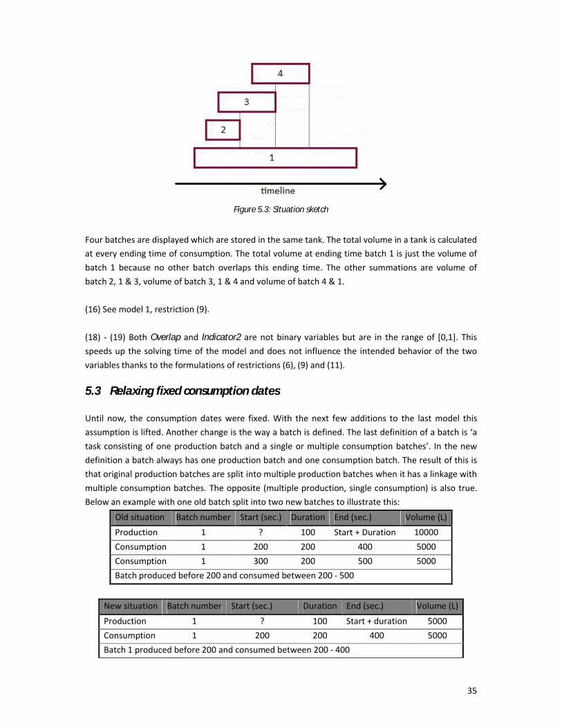
Figure 5.3: Situation sketch
Four batches are displayed which are stored in the same tank. The total volume in a tank is calculated at every ending time of consumption. The total volume at ending time batch 1 is just the volume of batch 1 because no other batch overlaps this ending time. The other summations are volume of batch 2, 1 & 3, volume of batch 3, 1 & 4 and volume of batch 4 & 1.
(16) See model 1, restriction (9).
(18) - (19) Both Overlap and Indicator2 are not binary variables but are in the range of [0,1]. This speeds up the solving time of the model and does not influence the intended behavior of the two variables thanks to the formulations of restrictions (6), (9) and (11).
5.3 Relaxing fixed consumption dates
Until now, the consumption dates were fixed. With the next few additions to the last model this assumption is lifted. Another change is the way a batch is defined. The last definition of a batch is ‘a task consisting of one production batch and a single or multiple consumption batches’. In the new definition a batch always has one production batch and one consumption batch. The result of this is that original production batches are split into multiple production batches when it has a linkage with multiple consumption batches. The opposite (multiple production, single consumption) is also true. Below an example with one old batch split into two new batches to illustrate this:
Old situation Batch number Start (sec.) Duration End (sec.) Volume (L)
Production 1 ? 100 Start + Duration 10000Consumption 1 200 200 400 5000Consumption 1 300 200 500 5000Batch produced before 200 and consumed between 200 - 500
New situation Batch number Start (sec.) Duration End (sec.) Volume (L)
Production 1 ? 100 Start + duration 5000Consumption 1 200 200 400 5000Batch 1 produced before 200 and consumed between 200 - 400

36
Production 2 Same as batch 1 100 Start + duration 5000Consumption 2 300 200 500 5000Batch 2 produced before 200 and consumed between 300 - 500
Mathematical modelThe extra sets, parameters, decision variables and constraints below are all extensions to the second MIP model with flexible production dates. Together it is one model in which the consumption dates are also flexible now.
Extra sets Index DescriptionSameConMachineb b Set of all other batches which use the same consumption
machine as batch bDiffProdBatchb b Set of all other batches which are not part of the same
‘original production batch’ (before splitting) as batch bSameProdBatchb b Set of all other batches which are part of the same
‘original production batch’ (before splitting) as batch bDiffConBatchb b Set of all other batches which are not part of the same
‘original consumption batch’ (before splitting) as batch bSameConBatchb b Set of all other batches which are part of the same
‘original consumption batch’ (before splitting) as batch b
Extra parameters Domain DescriptionDurationConsumptionb Batchb Duration (in seconds) of production batch bStartConsumptionb Batchb Starting time of consumption batch b, equal to
EndConsumptionb - DurationConsumptionb
Finishedb Batchb Latest possible time for a batch to be consumedBigMb Batchb Big-M equal to Finishedb - DurationConsumptionb
BigM2b Batchb Big-M equal to Finishedb
BigM3b’ Batch'b Big-M equal to Finishedb’ - DurationConsumptionb’
BigM4b’ Batch'b Big-M equal to Finishedb’ + 1
Extra dec. variables Domain DescriptionEndConsumptionb Batchb Ending time of consumption batch b
Indicator6b,b’bhineSameConMac'b
,Batchb
'bb
bb
0
1
batchnconsumptioof startthebeforefinishedisbatchof nconsumptioif
'batchnconsumptioof starttheafterfinishedisbatchof nconsumptioif
Model constraints & objective function Domain Nr.
Batchb
boductionPrEndMax (1)
s.t.

37
b'b,b'bb BigM*1IndicatoroductionPrStartoductionPrEnd
b
bodBatchPrDiff
odMachinePrSame'b,Batchb
(4)
11Indicator1Indicator b,'b'b,b
b
bodBatchPrDiff
odMachinePrSame'b,Batchb
(5)
b'b,b'bb 2BigM*6IndicatornConsumptioStarttionEndConsump
b
bchDiffConBat
hineSameConMac'b,Batchb
(23)
16Indicator6Indicator b,'b'b,b
b
bchDiffConBat
hineSameConMac'b,Batchb
(24)
'bb oductionPrEndoductionPrEnd bodBatchPrSame'b
,Batchb (25)
'bb tionEndConsumptionEndConsump bConBatchSame'b
,Batchb (26)
bb FinishedtionEndConsump Batchb (27)
1,06Indicator 'b,b bhineSameConMac'b
,Batchb (28)
0tionEndConsump b Batchb (29)
Explanation of the constraints
(23) - (24) A consumption machine can only have one task at a time. If two batches would have overlapping consumption tasks, then EndConsumptionb is higher than StartConsumptionb’ and EndConsumptionb’ is higher than StartConsumptionb. This results in b,'b'b,b 6Indicator6Indicator = 2
which is not allowed according to restriction (24). These restrictions are not needed for batches which have consumption tasks belonging to the same original consumption batch. They are assigned the same consumption dates by restriction (26) and thus do overlap.These restrictions are the reason for the redefinition of a batch. The old batch could have multiple consumption batches and thus, in reality, have multiple starting and ending dates of consumption. The starting time of consumption was set to the earliest starting time and the ending time of consumption was set to the latest ending time. Now with the restriction of non-overlapping machine (consumption) tasks this had to be changed. The new batch uses one consumption machine and has one starting and ending time for consumption.
(25) - (26) Batches are assigned the same ending time of production when they are part of the same original production batch. In reality they form one production batch. As a result of this, the domains of restrictions (4) & (5) are adjusted to this situation.Batches are assigned the same ending time of consumption too when they are part of the same original consumption batch.

38
(27) The ending time of consumption of a batch should be prior to the latest allowed ending time of consumption.

39
5.4 Results
In this section the results of the methods given the model specific assumptions will be presented.
The three MIP models are implemented in AIMMS 3.10 and are solved using the CPLEX 12.1 solver.
The variables of interest of the first model are the choice of tank (TankChoice) and the ending time of
production (EndProduction). In this FPDP problem each batch is stored in a single tank and a tank
never contains multiple batches. The ending time of production is shifted forward as much as
possible.
The results of model 1 for the three weeks of data can be seen in table 5.1. All three weeks are solved in a few seconds. It should be noted that the third week contains less batches then the other two weeks. Week three has 61 batches versus 99 and 93 batches for week one and two respectively.The objective values all show improvement when compared to the fixed total sum of ending times of production from the genetic algorithm. These summations were equal to 28035479, 25225137 and 16178466 for the three weeks.
FPDP Model 1 # variables # integers # constraints Objective value (sec.) solving time (sec.)
Week 1 22057 12255 75052 28636233 3Week 2 19581 10931 66366 26607495 4Week 3 8690 49684911 2952926052 17199420 1
Table 5.1: results FPDP model 1
In the second model (FPDP) it is allowed to store multiple batches in the same tank and to split batches and store them in different tanks. Regardless of this, table 5.2 shows that it does not change the objective values. Although the objective value did not change, the solutions show that batches are stored in other tanks. Figure 5.4 shows a Gantt chart for week 1. None of the batches overlap each other and also none of the batches are split and allocated to multiple tanks.
FPDP Model 2 # variables # integers # constraints Objective value (sec.) solving time (sec.)
Week 1 44827 22401 100224 28636223 12Week 2 40473 20005 90033 26607495 16Week 3 17335 8780 39017 17199420 1
Table 5.2: results FDPD model 2
In the third MIP model (FCDP) the consumption dates are not treated as being fixed anymore. The restriction is that the ending time needs to be before the latest allowed date (variable Finished). The variable Finished takes the value of the old fixed ending times of consumption. A consequence of flexible consumption dates is the new batch definition earlier described and with that an increase in the number of batches and also the number of variables in the model.

40
Letting the consumption dates be decision variables has a huge impact on the results as can be seen in table 5.3. For week 2 and 3 no solution is found within 24 hours. For week 3 the results are less bad with a solving time of 520 seconds.
Flexible consumption
# variables # integers # constraints Objective value (sec.) solving time (sec.)
Week 1 151421 73278 333708 - -Week 2 137805 66579 296639 - -Week 3 60575 28907 132536 17199420 520
Table 5.3: results model with flexible consumption
Next a test is performed on the maximum number of batches that can be scheduled within one minute solving time. First the batches are sorted on the former ending time of consumption which each batch had in the models with fixed consumption. Then the first ten batches are scheduled. If this succeeds another ten batches are added and so on until the solver fails to solve the batches within one minute. From this point the last added batch is removed until the solving time is below one minute. Table 5.4 shows the resulting number of batches which are scheduled.
Flexible consumption # batches Percentage (%) # variables # integers # constraints
Week 1 57 31 16877 7551 36990Week 2 59 34 18289 8113 39086Week 3 65 57 21673 9950 48760
Table 5.4: number of batches scheduled with solving time less than a minute

41
Figure 5.4: Gantt chart for week 1

42
6 Constraint programming approach
6.1 An introduction
Constraint programming is a programming methodology which is able to solve constraint satisfaction problems and combinatorial optimization problems. One of the main advantages of constraint programming is that you can represent problems explicitly in a natural and intuitive model. This is possible because of the type of constraints which are available for use. Examples are:
- logical constraints: if x is equal to 0, then y is also equal to 0
- global constraints: Constraints overlapping tasks: noOverlap(x), with x vector of intervals
- element constraints z = y(x(i)) Volume(i) ≤ Capacity(TankChoice(i)) with ‘i’ index of batch
It is not always self-evident to be able to linearize combinatorial optimization problems and to solve them with traditional mathematical programming methods. With the presence of above type of constraints in constraint programming this is no problem. Also with logical constraints there is no need for big-M formulations often used in MIP.
To explain how constraint programming works, we use definitions of IBM ILOG CP Optimizer documentation. IBM ILOG CP Optimizer is a constraint programming optimizer for solving detailed scheduling problems as well as combinatorial optimization problems that cannot be easily linearized and solved using traditional mathematical programming methods like MIP.
Constraint programming makes use of two techniques to find solutions for satisfaction / optimization problems: constructive search and constraint propagation. Before the search is started, initial constraint propagation performs domain reduction by removing possible values of decision variables that will never by part of a feasible solution. During search the engine of the solver in use will perform a constructive search strategy (branch and bound) in the reduced search space to find a feasible / optimal solution. Constraint propagation is performed before the search is started but also during search. During the branch and bound process temporary domains are created. Values are removed from these temporary domains by constraint propagation during search when they violate the constraints. An example of the search process is presented below. The example comes from the documentation of IBM’s ILOG CP Optimizer and is only slightly changed.
The problem is to find values for x and y from the following information:x + y = 17x - y = 5

43
x can be any integer from 5 through 12y can be any integer from 2 through 17
The initial constraint propagation removes values from domains that will not take part in any solution. Consider the constraint x + y = 17. If you take the smallest number in the domain of x, which is 5, and add it to the largest number in the domain of y, which is 17, the answer is 22. This combination of values (x = 5, y = 17) violates the constraint x + y = 17. The only value of x that would work with y = 17 is x = 0. However, there is no value of 0 in the domain of x, so y cannot be equal to 17. The value y = 17 cannot take part in any solution. The domain reduction algorithm employed by the constraint propagation engine removes the value y = 17 from the domain of y. Similarly, the propagation engine removes the following values from the domain of y: 13, 14, 15 and 16.
Likewise, if you take the largest number in the domain of x, which is 12, and add it to the smallest number in the domain of y, which is 2, the answer is 14. This combination of values (x = 12, y = 2) violates the constraint x + y = 17. The only value of x that would work with y = 2 is x = 15. However, there is no value of 15 in the domain of x, so y cannot be equal to 2. The value of y = 2 cannot take part in any solution. The propagation engine removes the value y = 2 from the domain of y. For the same reason, the domain reduction algorithm employed by the propagation engine removes the following values from the domain of y: 2, 3 and 4.
After initial propagation for the constraint x + y = 17, the domains are:D(x) = [5 6 7 8 9 10 11 12]D(y) = [5 6 7 8 9 10 11 12]
Now, examine the constraint x - y = 5. If you take the value 5 in the domain of x, you can see that the only value of y that would work with x = 5 is y = 0. However, there is no value of 0 in the domain of y, so x cannot equal 5. The value x = 5 cannot take part in any solution. The propagation engine removes the value x = 5 from the domain of x. Using similar logic, the propagation engine removes the following values from the domain of x: 6, 7, 8 and 9. Likewise, the domain reduction algorithm employed by the propagation engine removes the following values from the domain of y: 8, 9, 10, 11 and 12.
After initial propagation, the search space has been reduced in size. The domains are now:D(x) = [10 11 12]D(y) = [5 6 7]
After initial constraint propagation, the search space is reduced. The solver will use a constructive search strategy to guide the search for a solution in the remaining part of the search space. Suppose that, based on the search strategy, the optimizer has assigned the value 10 to the decision variable x. Working with the constraint x + y = 17, constraint propagation reduces the domain of y to [7]. However, this combination of values (x = 10, y = 7) violates the constraint x - y = 5. The optimizer removes the value y = 7 from the current domain of y. At this point, the domain of y is empty, and the optimizer encounters a failure. The optimizer can then conclude that there is no possible solution

44
with the value of 10 assigned to x. When the optimizer decides to try a different value for the decision variable x, the domain of y is at first restored to the values [5 6 7]. It then reduces the domain of y based on the new value assigned to x. The solver continues to search using constructive search and constraint propagation during search until a solution is found.

45
6.2 Implementation constraint programming
In this section several constraint programming formulations are presented. The formulations differ in the assumptions imposed on the tank scheduling problem. The program IBM ILOG OPL-CPLEX Analyst Studio is used for implementation. This program uses OPL (Optimization Programming Language), designed to substantially simplify optimization problems, as its programming language.
6.2.1 Basic modelsIn this subsection four models will be given which do not differ that much from each other. All four models treat the production and consumption processes as being fixed and have a feasible schedule as their goal. The difference is whether or not batches are allowed to be stored in multiple tanks and/or to store multiple batches in one tank at the same time. The specific assumptions of the four problems (BP) are respectively:
(1) Batches are stored completely in one tank and a tank can only contain one batch at a time.(2) Batches are stored completely in one tank and a tank may contain multiple batches at a time.(3) Batches are allowed to be allocated to multiple tanks for storage and a tank can only contain
one batch at a time.(4) Batches are allowed to be allocated to multiple tanks for storage and a tank may contain
multiple batches at a time.
The boxes below show the coding of the tank scheduling problem in OPL. The first box gives the sets, subsets and parameters used in the basic models. The corresponding names are adopted from the MIP section. The elements are initialized through a separate data file replacing the dots.
//setsint nbBatches = ...; //number of batchesint nbTanks = ...; //number of tanks
//parametersint Capacity[1..nbTanks] = ...; //Capacityint Volume[1..nbBatches] = ...; //Volumeint Product[1..nbBatches] = ...; //Product typeint StartProduction[1..nbBatches] = ...; //Starting time productionint EndProduction[1..nbBatches] = ...; //Ending time productionint StartConsumption[1..nbBatches] = ...; //Starting time consumptionint EndConsumption[1..nbBatches] = ...; //Ending time consumptionint TankOption[1..nbBatches][1..nbTanks] = ...; //Available tanks
//subsets//tanks available for batch b:{int} AvailableTanks[b in 1..nbBatches] = {t | t in 1..nbTanks:
TankOption[b][t] == 1};//tanks not available for batch b:{int} NonAvailableTanks[b in 1..nbBatches] = {t | t in 1..nbTanks:
TankOption[b][t] == 0};//batches with a different product type than batch b:{int} DiffProduct[b in 1..nbBatches] = {j | j in 1..nbBatches: Product[b]
!= Product[j]}; //batches with the same product type as batch b:

46
{int} SameProduct[b in 1..nbBatches] = {j | j in 1..nbBatches: Product[b]== Product[j]};
Basic model (1)In constraint programming working with an objective function is allowed but not always required. In this and the other basic models the objective function is not included because the goal of a feasible scheduled does not require this.The only decision variable needed in the model is the choice of tank (TankChoice). Because of the ability to use logical constraints, no other decision variables are needed. The value of TankChoice is restricted to be in the range 1, .., nbTanks. Next to that the first restriction reduces the domain of TankChoice to the set of available tanks.The second restriction ensures that batches are stored in tanks with enough capacity. A decision variable is used as an index to retrieve the capacity of the selected tank. Something which would not be possible in linear programming. The third restriction states, if two batches are stored in the same tank, then they are not allowed to overlap in time. The symbol ‘=>’ used has the meaning ‘imply’ and not ‘greater than or equal to’.
//decision variables//Tank used to store batch b:dvar int TankChoice[b in 1..nbBatches] in 1..nbTanks;
//Restrictionssubject to { forall(b in 1..nbBatches, t in NonAvailableTanks[b]) TankChoice[b] != t;
forall(b in 1..nbBatches) Volume[b] <= Capacity[TankChoice[b]];
forall(b in 1..nbBatches, j in 1..nbBatches: j > b) TankChoice[b]==TankChoice[j] => EndConsumption[b] >
StartProduction[j] || StartProduction[b] < EndConsumption[j];}
Basic model (2)Restriction two is changed to cope with multiple batches stored in one tank. It has the same function as restrictions (13) - (15) of the second MIP model. The left part of the restriction calculates the volume of batch b plus the volume of all other batches (with the same choice of tank and product type) whose ending time of consumption falls between the starting time of production of batch band its ending time of consumption. This calculated volume has to be less than or equal to the capacity of the tank in question.The third restriction states, if two batches are stored in the same tank and contain different product types, then they are not allowed to overlap in time.
//decision variables//Tank used to store batch b:dvar int TankChoice[b in 1..nbBatches] in 1..nbTanks;
//Restrictionssubject to { forall(b in 1..nbBatches, t in NonAvailableTanks[b])

47
TankChoice[b] != t;
forall(b in 1..nbBatches) Volume[b] + sum(j in SameProduct[b]) Volume[j] * (EndConsumption[b] >
EndConsumption[j] && StartProduction[b] < EndConsumption[j] && TankChoice[b]==TankChoice[j]) <= Capacity[TankChoice[b]];
forall(b in 1..nbBatches, j in DiffProduct[b]: j > b) TankChoice[b]==TankChoice[j] => EndConsumption[b] >
StartProduction[j] || StartProduction[b] < EndConsumption[j];
}
Basic model (3)In the third model it is possible to store a batch in multiple tanks. The variable TankChoice is replaced by the new decision variable VolumeDistribution. This variable describes how much volume of batch b is in tank t. Restriction one states that the volume of batch b should be stored in one or more of its available tanks. Again the second restriction ensures that batches are stored in tanks with enough capacity. The third restriction prevents overlapping batches. If a batch has an overlap in time with another batch, then these batches will to be stored in different tanks.
//decision variablesdvar int VolumeDistribution[b in 1..nbBatches][t in 1..nbTanks] in
0..Volume[b];//Restrictionssubject to { forall(b in 1..nbBatches, t in AvailableTanks[b]) sum(t in 1..nbTanks) VolumeDistribution[b][t] == Volume[b];
forall(b in 1..nbBatches, t in AvailableTanks[b]) VolumeDistribution[b][t] <= Capacity[t]; forall(b in 1..nbBatches, j in 1..nbBatches: j > b, t in
AvailableTanks[b]) VolumeDistribution[b][t] > 0 && VolumeDistribution[j][t] > 0 =>
EndConsumption[b] > StartProduction[j] || StartProduction[b] <EndConsumption[j];
}
Basic model (4)The last basic model uses the same decision variable as model 3. It also copies restriction one. Restriction two and three are almost copies of the second and third restriction of model 2. An extra domain ( banksAvailableTt ) is added and the variable TankChoice is replaced by
VolumeDistribution for both restrictions.
//decision variablesdvar int VolumeDistribution[b in 1..nbBatches][t in 1..nbTanks] in
0..Volume[b];//Restrictionssubject to { forall(b in 1..nbBatches, t in AvailableTanks[b]) sum(t in 1..nbTanks) VolumeDistribution[b][t] == Volume[b];
forall(b in 1..nbBatches, t in AvailableTanks[b]) VolumeDistribution[b][t] + sum(j in SameProduct[b])
VolumeDistribution[j][t] * (EndConsumption[b] > StartProduction[j] &&

48
StartProduction[b] < StartProduction[j]) <= Capacity[t];
forall(b in 1..nbBatches, j in DiffProduct[b]: j > b, t inAvailableTanks[b])
VolumeDistribution[b][t] > 0 && VolumeDistribution[j][t] > 0 =>EndConsumption[b] > StartProduction[j] || StartProduction[b] <
EndConsumption[j];}
6.2.2 Extended modelThe aim of the extended model is to obtain a feasible schedule and execute the productions as late as possible (FPDP). This means that production dates are not fixed now. The model can be divided into four models under different situations (assumptions), just like with the basic model. The choice here is to only provide the extended version of basic model 1, because the other three can be obtained by some small changes similar to the changes in the basic models.
The aim of this model requires an objective function in the formulation. The objective function ofcourse is the same as in the MIP models; maximize the sum of all ending times of production. The consequence of giving up fixed production dates is that restrictions need to be added to prevent machines from having multiple tasks at the same time. With ‘noOverlap’ OPL has a predefined constraint for this. It prevents intervals (starting time production - ending time production) from overlapping.The code: noOverlap(all (i in SameProdMachine[b]) ProdBatches[i]);
means that all production batches, which use the same production machine, are not allowed to have overlapping production processes. Prodbatches here is an interval variable with a starting- and ending time and with starting time plus duration equaling ending time. The starting- and ending time of production can be accessed by stating startOf(ProdBatches[b]) and endOf(ProdBatches[b]) respectively.
//Extra parametersstring ProdMachine[1..nbBatches] = ...;int DurationProduction[1..nbBatches] = ...;
//Extra subset//batches which use the same production machine as batch b:{int} SameProdMachine[b in 1..nbBatches] = {j | j in 1..nbBatches:
ProdMachine[b] == ProdMachine[j]};
//decision variablesdvar int TankChoice[b in 1..nbBatches] in 1..16;dvar interval ProdBatches[b in 1..nbBatches] in 0..StartConsumption[b] size
DurationProduction[b];//expression variablesdexpr int StartProduction[b in 1..nbBatches] = startOf(ProdBatches[b]);dexpr int EndProduction[b in 1..nbBatches] = endOf(ProdBatches[b]);
maximize sum(b in 1..nbBatches) EndProduction[b];
subject to { forall(b in 1..nbBatches, t in NonAvailableTanks[b])

49
TankChoice[b] != t;
forall(b in 1..nbBatches) noOverlap(all (i in SameProdMachine[b]) ProdBatches[i]);
forall(b in 1..nbBatches) Volume[b] <= Capacity[TankChoice[b]];
forall(b in 1..nbBatches, j in 1..nbBatches: j > b) TankChoice[b]==TankChoice[j] => EndConsumption[b] >
StartProduction[j] || StartProduction[b] < EndConsumption[j];}

50
6.3 Results
This section presents the results of the constraint programming models. As earlier stated the models are implemented in IBM ILOG OPL-CPLEX Analyst Studio. The solver used here is IBM ILOG CP Optimizer, according to IBM, their next generation constraint programming engine for solving sequencing, resource allocation and timetabling problems that are difficult or impossible to solve with mathematical programming based techniques.
Tables 6.1-6.4 show the results for the four BP’s and their accompanying basic models. All models solve the problem within one second for each week. The models do not have an objective function and therefore the table does not give values on them.
Basic Model 1 # variables # constraints Objective value (sec.) solving time (sec.)
Week 1 99 25508 - < 1Week 2 93 22571 - < 1Week 3 61 9917 - < 1
Table 6.1: results basic model 1
Basic Model 2 # variables # constraints Objective value (sec.) solving time (sec.)
Week 1 99 26570 - < 1Week 2 93 23720 - < 1Week 3 61 10389 - < 1
Table 6.2: results basic model 2
Basic Model 3 # variables # constraints Objective value (sec.) solving time (sec.)
Week 1 1584 131747 - < 1Week 2 1488 112841 - < 1Week 3 976 48699 - < 1
Table 6.3: results basic model 3
Basic Model 4 # variables # constraints Objective value (sec.) solving time (sec.)
Week 1 1584 133196 - < 1Week 2 1488 114056 - < 1Week 3 976 49518 - < 1
Table 6.4: results basic model 4
Table 6.5 gives the result of the extended model (FPDP). Batches are stored completely in one tankand a tank can only contain one batch at a time. CP Optimizer is not able to find the optimal solution

51
within one hour for week 1 and week 2. But is does find feasible solutions within one minute solving time which are near optimal.
Extended Model # variables # constraints Objective value (sec.) solving time (sec.) Time limit
Week 1 198 25608 28636064 57 1 hourWeek 2 186 22665 26606670 52 1 hourWeek 3 122 9979 17199420 9 1 hour
Table 6.5: results extended model
For week 1, the only difference between the optimal solution (first MIP model) and the near optimal found here is shown in figure 6.1. The picture shows two production tasks on a single machine. Looking at the ending times of production, the optimal solution is preferred over the near optimal solution. But looking at the schedule of the two production batches taken as a whole, neither of the two is preferred over the other.
Figure 6.1: CP solution vs. MIP solution
For week 2, all production dates in the solution are the same as the production dates of the first two MIP model solutions, except for five of them. These five productions use the same production machine and therefore are not allowed to overlap in time. Figure 6.2 shows the situation for the optimal solution and the near optimal solution from the CP-model. The ending time of production of batch 5 is equal to its starting time of consumption in the optimal solution meaning it can not be shifted to the right anymore. The same holds true for batch 4 in the near optimal solution. The optimal solution is optimal according to the value of the objective function, but looking at the picture you could say the near optimal solution is at least as good in terms of tank occupation. When the objective function is changed to the sum of ending times consumption minus the sum of starting times productions, then both displayed solutions below would have the same value.
Figure 6.2: CP solution vs. MIP solution

52
CP Optimizer does find the optimal solution of week 3 in 9 seconds, but it is not able to prove that it is the best possible solution. This sounds weird, but the solution found has the same objective value as the objective value (proven optimal) of the first two MIP models. Therefore this solution has to be optimal.
The last results are under the assumptions that batches are stored completely in one tank and a tank can only contain one batch at a time. The other three situations described in 6.2.1 (Basis models) are also implemented but do not provide good results in terms of solving time and quality of feasible solutions.

53
7 Conclusions and recommendations
The goal of this thesis was to solve tank scheduling by using different techniques and to compare the limitations and the results of each technique. The choice was made to implement a genetic algorithmwith and without variable population size, mixed integer programming models and constraint programming models. Also a greedy algorithm based on the SA approach from Bui et al. (2009) has been implemented.
The genetic algorithms with and without varying population size showed to be having trouble finding a feasible schedule. Three datasets were used for computational testing and especially the second set gave problems for the genetic algorithms. The GAVaPS outperformed the GA with fixed population size but still only managed to create feasible tank schedules in 63% of the runs for the second week of data. The greedy algorithm turned out to be more successful. It had no difficulty solving tank scheduling problems within a short amount of time.
The former algorithms solved problems under the assumption of fixed production and consumption dates. The assumption of fixed production was lifted for all three MIP models and also the consumption dates were flexible for the third MIP model. The MIP models with fixed consumption dates were able to schedule all the batches within 20 seconds for all datasets. Treating consumption dates as decision variables lead to a MIP model in which the number of variables increased with a factor of at least three due to a needed change in the definition of a batch. As a result, this MIP model was only able to schedule a subset of the batches.
CP, the last technique used to solve tank scheduling problems, provided very good results for the four basic problems with a solving time less than a second. The extended CP model (FPDP) gave different results. In this model assumptions of batches which need to be stored in one tank and a tank may not contain multiple batches are needed for CP to create a feasible schedule within one minute.
It can be concluded that greedy algorithm, MIP and CP approaches are successful in solving tank scheduling problems. Greedy algorithms and CP are preferred for fixed production and consumption date problems due to their ease of implementation and short solving times. Both these approaches are limited in the sense that the greedy algorithm is not able to treat production and/or consumption dates as flexible and CP already has some difficulties in scheduling batches with flexible production dates. Therefore, CP is not expected to provide good results when also the consumption dates would be flexible. Looking at the results MIP approaches are a good choice when production dates are flexible and are the best choice among the different techniques when consumption dates are also flexible.
For further research it could be interesting to explore CP approaches to tank scheduling some more. It not only provided good results in this thesis but it is also very easy to use in general thanks to the

54
intuitive model representation. Providing customized search strategies could be an option to deal with more difficult problems.In the ideal situation you would have a technique able solve tank scheduling problems in which tanks and machines are scheduled simultaneously. Whether this is possible with the current solution techniques and solvers, remains unknown as it is too complex for the moment. Further investigation and improvement of solvers should tell.

55
References1. Arabas, J., Michalewicz, Z. and Mulawka, J. (1994) “GAVaPS: a genetic algorithm with varying
population size”, Proceedings of the First IEEE Conference on Evolutionary Computation, 73-78.
2. Bossers, H., Broch, R., Oosterom, C. van and Veelenturf, L. (2009). “Tank scheduling at FrieslandCampina”, Report Case Studies 2, Erasmus University Rotterdam.
3. Bui, V., Glorie, K., Parlevliet, T., Salonikidis, K. (2009). “A Simulated Annealing Approach for Tank Scheduling at Friesland-Campina”, Report Case Studies 2, Erasmus University Rotterdam.
4. Broch, R.P.J. (2008). “Tank scheduling met mixed integer linear programming”, Bachelor thesisEconometrics and Operational Research.
5. Colorni, A., Dorigo, M. and Maniezzo, V. (1991). “Genetic Algorithms and Highly ConstrainedProblems: The Time-Table Case”, Proceedings of the First International Workshop on Parallel Problem Solving from Nature, Lecture Notes in Computer Science 496, 55-59.
6. Colorni, A., Dorigo, M. and Maniezzo, V. (1998). “Metaheuristics for high-school timetabling”, Computational Optimization and Applications 9, 275-298.
7. Glibovets, N.N. and Medvid, S.A. (2003). “Genetic Algorithms Used to Solve SchedulingProblems”, Cybernetics and Systems Analysis 39, No. 1, 81-90.
8. Gomes, C.P., Hoeve. W.-J. van, Lombardi, M. and Selman, B. (2007). “Optimal Multi-Agent Scheduling with Constraint Programming”, In Proceedings of the Nineteenth Conference on Innovative applications of Artificial Intelligence.
9. Grossmann, I.E., Jain, V. (2000). “A Disjunctive Model for Scheduling in a Manufacturing and Packing Facility with Intermediate Storage”, Optimization and Engineering 1, 215-231.
10. Hancock, P.J.B. (1994). “An empirical comparison of selection methods in evolutionary algorithms”, AISB Workshop on Evolutionary Computing, Lecture Notes in Computer Science 865,80-94.
11. IBM, Getting Started with IBM ILOG CP Optimizer
12. Kallrath, J. (2002). “Planning and Scheduling in the Process Industry”, OR Spectrum 24, pp. 219-250.
13. Li, T., Li, Y., Zhang, Q., Gao, X. and Dai, S. (2005) “Constraint Programming Approach toSteelmaking-making Process Scheduling”, Communications of the IIMA 5, Issue 3.
14. Karray, F. O. and De Silva, C (2004). Soft Computing and Intelligent Systems Design, Theory, Tools, and Applications. Essex, Pearson Education Limited.
15. Michalewicz, M. (1996). Genetic Algorithms + Data Structures = Evolution Programs. 3rd ed. Germany, Springer-Verlag.
16. Verbiest, W.J. (2008). “Tank Scheduling with Cost/Profit Optimization”, Master thesis, Erasmus University Rotterdam.

56
17. Whitley, D. (1989). “The GENITOR Algorithm and Selection Pressure: Why Rank-Based Allocation of Reproductive Trials is Best”, Proceedings of the 3rd International Conference on Genetic Algorithms, 116-121.
18. Yao, X. (1997). “Global optimisation by Evolutionary Algorithms”, International Symposium on Parallel Algorithm/Architecture Synthesis, 282-291.