multiple outcomes of speculative behavior in theory and in ... · multiple outcomes of speculative...

Multiple Outcomes of Speculative Behavior in

Theory and in the Laboratory1

James S. CostainUniv. Carlos III de Madrid

Frank Heinemann

Ludwig-Maximilians-Universitat, MunchenGoethe-Universitat, Frankfurt am Main

Peter OckenfelsGoethe-Universitat, Frankfurt am Main

First version: July 2004This version: April 2005

PRELIMINARY

Correspondence address:Department of Economics

Universidad Carlos III de MadridCalle Madrid 126

28903 Getafe (Madrid), [email protected]

1Thanks to Rosemarie Nagel and Dan Friedman for helpful discussions. The experimentsdescribed in this paper were programmed and conducted with the z-Tree software package(Urs Fischbacher, Univ. of Zurich, 1999). Financial support from the Spanish Ministry ofScience and Technology (MCyT grant SEC2002-01601) is gratefully acknowledged. Errorsare the responsibility of the authors. Raw data, additional graphs, and other experimentaland numerical materials can be found at http://www.econ.upf.es/∼costain/cho/cho.html.

Abstract

This paper shows that Morris and Shin’s (AER 1998) argument that the out-come of a speculative attack is uniquely determined by macroeconomic funda-mentals fails if decisions are not simultaneous. As long as most agents observethe choices of a few others before making their own decisions, we find thatthere is a range of fundamentals where multiple outcomes occur, as Obstfeld(1996) claimed.

Theoretically, we show that if most players observe many others beforechoosing, then the distribution over aggregate outcomes is close to the distri-bution implied one of the symmetric-information sunspot equilibria. In ourexperimental sessions, eight to sixteen players observe signals about the aggre-gate state and may also observe a random subset of previous actions. We finda unique mapping between fundamentals and the fraction of players attack-ing if previous actions are unobserved. But when most previous actions areobserved, there is an intermediate interval of fundamentals (which is usuallystatistically significant) where all players attacking, and no players attacking,both occur with more than 1% probability.

JEL classification: C62, C72, C73, C92, E00, F32Keywords: Multiplicity, herding, global games, currency crises, experi-

ments

1

1 Introduction

In an influential paper, Morris and Shin (AER 1998, henceforth MS98) have

argued that because of imperfect information, speculation against a fixed ex-

change rate is likely to yield a unique outcome for any given state of macroe-

conomic fundamentals. This paper challenges their conclusion, showing that

it relies heavily on an assumption of exactly simultaneous choice. We show

that if players have a sufficiently high probability of observing a few previous

actions before making their own decisions, then there exists a range of fun-

damentals over which multiple self-fulfilling outcomes occur.1 In other words,

sequential choice brings back the more traditional “tripartite classification of

fundamentals”, as illustrated in Figure 1, that occurs in models like that of

Obstfeld (1996).

MS98 is an example of a more general uniqueness result that arises under

imperfect information in the context of “global games”, as defined by Carlsson

and van Damme (1993). The result is surprisingly widely applicable (Morris

and Shin 2003; Frankel, Morris, and Pauzner 2003), though it relies on private

information being sufficiently accurate relative to public information (Hellwig

2002; Tarashev 2001). Heinemann, Nagel, and Ockenfels (2004; henceforth

HNO04) find uniqueness in laboratory experiments based on MS98, as do

Cabrales, Nagel, and Armenter (2002) for a related game. However, they find

no evidence for the differences between complete and incomplete information

settings that the global games framework implies.

Chamley (2003A) and Costain (2003) argue that multiplicity may be re-

stored if choice is not exactly simultaneous. Sequential choice in the presence

of imperfect information and/or strategic complementarities may allow herd-

ing behavior to produce multiple outcomes in the same aggregate state, as in

Banerjee (1992), Bikhchandani, Hirshleifer, and Welch (1992, 1996), Cham-

ley (2003A, 2003B), and Chari and Kehoe (2003). Anderson and Holt (1997)

1It is important to emphasize that the primary focus of this paper is multiplicity ofmacroeconomic outcomes conditional on aggregate fundamentals— which we believe is therelevant issue for policy makers— rather than the related but more theoretical question ofmultiplicity of equilibrium.

2

demonstrate herding behavior in the laboratory. Costain (2003) studies the ef-

fects of both imperfect information and strategic complementarities in a game

with both global game and herding aspects. His overall conclusion is that the

uniqueness induced by the global games structure is fragile, while the multi-

plicity induced by herding is robust, and leads to a probability distribution

resembling a sunspot equilibrium.

This paper generalizes MS98 to allow non-simultaneous choice, by applying

Costain’s herding structure to the MS98 game. Since some previous choices are

observed, the complicated iterated dominance calculations that players must

perform in a simultaneous game become less relevant, making it optimal for

most players to just follow the crowd. But therefore the MS98 uniqueness re-

sult breaks down: in some aggregate states, the choice of the first few players

has a decisive impact on the choice of the rest, allowing multiple aggregate

outcomes to occur with positive probability. In fact, the macroeconomic be-

havior of the model is similar to that generated by a sunspot equilibrium. To

be precise, as the average number of observations increases, the equilibrium

distribution of outcomes of our herding model converges to the distribution

associated with one of the model’s symmetric-information sunspot equilibria.

And while this analytical result refers to a limit with many observations, we

find numerically that the model generates self-fulfilling multiplicity like that

of a sunspot equilibrium even when the number of agents or the number of

observations is small. Likewise, in our laboratory experiments, players tend to

follow the crowd. Therefore, with eight players and 75% probability of observ-

ing previous plays, we observe a range of fundamentals in which the fraction

of players attacking has a bimodal distribution.

2 The herding model

2.1 Morris and Shin’s game

Our intention here is to construct a game as close as possible to MS98’s stylized

model of speculative attacks, except that choice is not exactly simultaneous.

In their game, many individual traders decide whether or not to attack a

3

currency peg, on the basis of limited information about the true state Θ of

the macroeconomy. If the proportion of traders who choose to attack exceeds

a hurdle function a(Θ), devaluation occurs, resulting in a payoff R(Θ) − t to

the attackers. Otherwise, attackers lose the transactions cost t. Players who

choose not to attack have payoff zero. It is assumed that a′ > 0 and R′ < 0,

so that larger Θ represents a better state of the economy.

Ex ante, the fundamental state Θ has the c.d.f. G(Θ), which is assumed to

be a uniform distribution over the support [θ, θ]. To ensure that the problem

is interesting, we assume parameters that guarantee a “tripartite classification

of fundamentals” under full information. Let I be the number of players.

Assumption 1. a. If the state is sufficiently bad, it is worthwhileto attack: R(θ)/t > 1 and a(θ) < 1/I.

b. If the state is sufficiently good, it is worthwhile not to attack:R(θ)/t < 1 or a(θ) > 1.

c. There is a non-empty interval of θ ∈ [θ, θ] such that a fullinformation game of simultaneous moves would have multipleequilibria: R(θ)/t > 1 and 1/I < a(θ) < 1.

In Morris and Shin’s model, however, information is incomplete. Player i’s

information about Θ comes as a signal xi, which is i.i.d. across individuals,

with a conditional c.d.f. F (xi|Θ) that is uniform on [Θ − ε, Θ + ε]. 2

2.2 Sequential choice

We list the I players as i ∈ II ≡ {1, 2, 3, . . . , I}.3 Individuals make their

decisions in numerical order, choosing actions ηi from the binary set {0, 1}.

2Numerically and experimentally, we must restrict variables to finite, discrete supports.Thus we assume that the support of Θ is an equally-spaced grid from θ to θ, and that theconditional support of xi is an equally-spaced grid from Θ − ε to Θ + ε.

3Costain (2003) focuses on the limiting case I = ∞, which simplifies the structure ofthe equilibrium; but here we also consider the finite I case, for compatibility with ourexperiments.

4

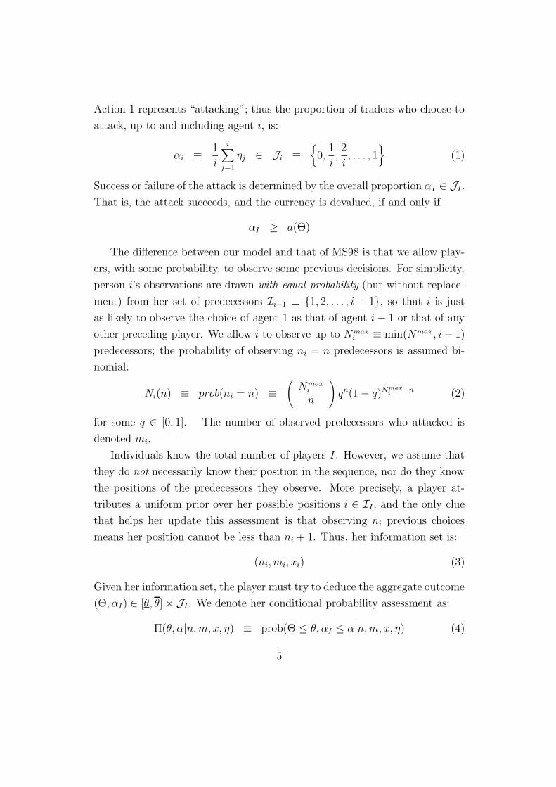
Action 1 represents “attacking”; thus the proportion of traders who choose to

attack, up to and including agent i, is:

αi ≡1

i

i∑

j=1

ηj ∈ Ji ≡{

0,1

i,2

i, . . . , 1

}

(1)

Success or failure of the attack is determined by the overall proportion αI ∈ JI.

That is, the attack succeeds, and the currency is devalued, if and only if

αI ≥ a(Θ)

The difference between our model and that of MS98 is that we allow play-

ers, with some probability, to observe some previous decisions. For simplicity,

person i’s observations are drawn with equal probability (but without replace-

ment) from her set of predecessors Ii−1 ≡ {1, 2, . . . , i − 1}, so that i is just

as likely to observe the choice of agent 1 as that of agent i − 1 or that of any

other preceding player. We allow i to observe up to Nmaxi ≡ min(Nmax, i − 1)

predecessors; the probability of observing ni = n predecessors is assumed bi-

nomial:

Ni(n) ≡ prob(ni = n) ≡

(

Nmaxi

n

)

qn(1 − q)Nmax

i−n (2)

for some q ∈ [0, 1]. The number of observed predecessors who attacked is

denoted mi.

Individuals know the total number of players I. However, we assume that

they do not necessarily know their position in the sequence, nor do they know

the positions of the predecessors they observe. More precisely, a player at-

tributes a uniform prior over her possible positions i ∈ II , and the only clue

that helps her update this assessment is that observing ni previous choices

means her position cannot be less than ni + 1. Thus, her information set is:

(ni, mi, xi) (3)

Given her information set, the player must try to deduce the aggregate outcome

(Θ, αI) ∈ [θ, θ] × JI . We denote her conditional probability assessment as:

Π(θ, α|n, m, x, η) ≡ prob(Θ ≤ θ, αI ≤ α|n, m, x, η) (4)

5

Note that the individual’s choice η influences the perceived distribution of the

aggregate outcome αI , except perhaps in the limiting case I = ∞.

In general, individuals could choose a mixed strategy, playing η = 1 with

probability y(n, m, x) conditional on any idiosyncratic state (n, m, x). How-

ever, generically, players will strictly prefer 0 or 1 for almost every (n, m, x).

Therefore, in our simulations we search for threshold functions τ(n, m) repre-

senting the signals at which players are indifferent between attacking or not.

Since a higher x indicates a better fundamental state Θ, and thus a lower payoff

to attacking, we expect to find threshold equilibria of the following form:

y(n, m, x) = 1 iff x ≤ τ(n, m)y(n, m, x) = 0 iff x > τ(n, m)

but we will also check whether this is in fact optimal in our simulations. The

threshold signal τ(n, m) must satisfy the indifference condition

t = EΠ

[

R(Θ)1αI≥a(Θ)|n, m, τ(n, m), η = 1]

(5)

Here 1X is an index function taking the value 1 if statement X is true, and

0 otherwise. This first-order condition equates the cost t of attacking to its

expected payoff, which is R(Θ) as long as the fraction αI attacking exceeds the

hurdle a(Θ). The expectation is evaluated using the probability distribution

Π, conditional on observing n agents, of whom m attacked, and signal x =

τ(n, m), and also conditional on playing η = 1.

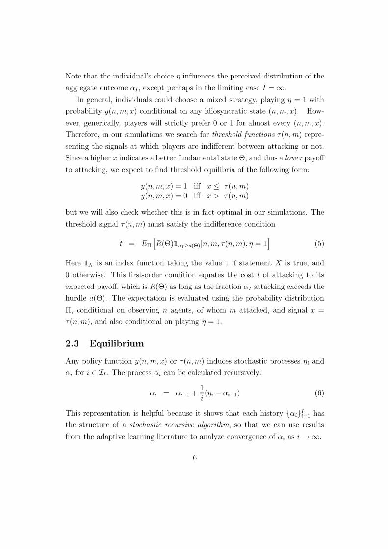
2.3 Equilibrium

Any policy function y(n, m, x) or τ(n, m) induces stochastic processes ηi and

αi for i ∈ II . The process αi can be calculated recursively:

αi = αi−1 +1

i(ηi − αi−1) (6)

This representation is helpful because it shows that each history {αi}Ii=1 has

the structure of a stochastic recursive algorithm, so that we can use results

from the adaptive learning literature to analyze convergence of αi as i → ∞.

6

To spell out the stochastic processes for ηi and αi, recall first that the c.d.f.

of the aggregate fundamental is G(Θ). Next, for each i ∈ I, a signal xi is

drawn with distribution F (x|Θ). The number of observations ni is drawn with

distribution Ni(n). These observations are drawn randomly from the set of

predecessors (without replacement). Therefore, if the fraction of predecessors

who have attacked is αi−1 = α, then the probability of observing exactly m

attackers in a sample of ni = n predecessors, is

Mi(m|n, α) ≡ prob(mi = m|i, n, α) ≡

(

α(i − 1)m

)(

(1 − α)(i − 1)n − m

)

(

i − 1n

) (7)

which goes to M(m|n, α) ≡

(

nm

)

αm(1 − α)n−m ≡ n!m!(n−m)! αm(1 − α)n−m

in the limit as i increases (see Berck and Sydsaeter (), page ??).

Given the individual state (ni, mi, xi), player i’s choice is ηi = 1 if xi is

less than or equal to the threshold τ(ni, mi), and zero otherwise. This implies

an explicit formula for the probability that ηi = 1, given the fraction αi−1 of

predecessors who attacked, the index i, the state Θ, and the policy τ():

Ti(αi−1, Θ, τ()) ≡ prob(ηi = 1|i, αi−1, Θ, τ()) = (8)

Nmax

i∑

n=0

Ni(n)n∑

m=0

Mi(m|n, αi−1)F (τ(n, m)|Θ)

For large i, Nmaxi = Nmax and Mi(m|n, α) → M(m|n, α), so the sequence of

functions Ti approaches a limit T (α, Θ, τ()). Note that M and therefore T are

C∞ functions of α.

The function Ti states the probability that trader i attacks the currency,

given the fraction who attacked prior to him. Using Ti, we can construct all

the other probabilities that are needed to solve the model. In particular, we

need the following joint probability (for details, see Section 4):

prob(αI , Θ, i, ni, mi, xi, |ηi = 1, τ)

7

which means the joint probability of the event in which the the aggregate

outcome is (αI , Θ), the individual position is i, and individual information set

is (ni, mi, xi), assuming that all other players use strategy τ and the individual

chooses ηi = 1. Knowing this joint probability, the trader can construct the

conditional distribution he needs to solve his maximization problem:

Π(α, θ|n, m, x, η = 1) =

∑

i,αI≤α,Θ≤θ prob(αI , Θ, i, n, m, x, |η = 1, τ)∑

i,αI ,Θ prob(αI , Θ, i, n, m, x, |η = 1, τ)(9)

The conditional probability distribution in (9) is all the information nec-

essary to choose an optimal threshold strategy. Thus we can define a herding

equilibrium as a pair (τ, Π) such that:

1. If all others play strategy τ , then the conditional probabilitydistribution given by (9) is Π.

2. If the probability distribution over aggregate outcomes (αI , Θ),conditional on individual information (n, m, x) and individualchoice η = 1 is Π, then the individual’s preferred strategy is τ(that is, τ solves (5)).

While Π is the most useful distribution for solving the model, and could in

principle be observed in the laboratory, it cannot be observed with macroeco-

nomic data. The observable implications of the model in terms of macroeco-

nomic data are summarized by the distribution over aggregate outcomes. We

will use the notation P (αI, Θ) to represent this distribution; more specifically,

P refers to the joint c.d.f. over fundamentals Θ and the fraction attack-

ing αI . We will also use the notation p(αI |θ) to refer to the probability of

αI ∈ {0, 1/i, 2/i, ...1} conditional on the aggregate state θ. Figures 2-5 illus-

trate numerical simulations and experimental counterparts of the conditional

probability p (first as a 3d plot, and then as a contour plot).

3 Limiting results

To better understand the distribution of aggregate outcomes generated by this

model, it is helpful to consider the limit of the game as the number of players

increases without bound. For I = ∞, the fact that αi is a stochastic recursive

8

algorithm means that the outcomes α∞ ≡ limI→∞1I

∑Ii=1 ηi which are possible

conditional on a given state θ must lie in a small set of points consistent with

the concept of “E-stability” in the sense of Evans and Honkapohja (2001).4

Using our previous notation, any α∞ which occurs with positive probability, if

interior, must be a point where T crosses the 45o line from above. Intuitively, a

given α∞ is possible if the probability that individual i attacks, conditional on

fraction α∞ attacking before him, converges to α∞ as i → ∞. Corner solutions

are also possible: α∞ = 0 is a solution if T is zero at α = 0, and α∞ = 1 is a

solution if T is one at α = 1.

Thus, conditional on a given aggregate state Θ = θ, and on equilibrium

strategy τ ∗, the set of possible outcomes α∞ of the I = ∞ model is a set of

discrete points: those points where T (α, θ, τ ∗) crosses the 45o line from above,

plus any appropriate corners. There may be only one such point, which means

that the aggregate outcome is unique conditional on the aggregate fundamental

θ. But there may also be multiple crossings and/or corners for some θ, in

which case there are multiple aggregate outcomes that occur with positive

probability conditional on that aggregate state θ. Typically there is either one

possible aggregate outcome (when T is mildly upward-sloping) or two possible

aggregate outcomes (when T is S-shaped).

The model’s behavior can also be clarified by studying what happens as

the average number of observations gets large. Thus, fix I = ∞ and fix q, and

let the maximum number of observations Nmax increase without bound.

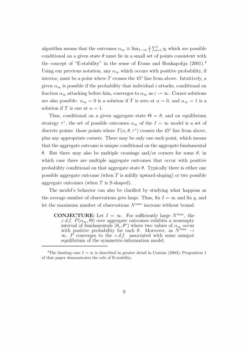
CONJECTURE: Let I = ∞. For sufficiently large Nmax, thec.d.f. P (α∞, Θ) over aggregate outcomes exhibits a nonemptyinterval of fundamentals (θ∗, θ

∗) where two values of α∞ occurwith positive probability for each θ. Moreover, as Nmax →∞, P converges to the c.d.f. associated with some sunspotequilibrium of the symmetric-information model.

4The limiting case I = ∞ is described in greater detail in Costain (2003); Proposition 1of that paper demonstrates the role of E-stability.

9

KEY POINTS IN PROVING THIS CONJECTURE:1. Pick γ ∈ (0, 0.5). For any equilibrium, define

θ∗ ≡ inf{θ : α∞ ≥ a(θ) with probability > γ}

θ∗ ≡ sup{θ : α∞ < a(θ) with probability > γ}

Thus θ∗ is the lowest aggregate state such that there is not a successful attackwith at least probability γ, while θ∗ is the highest aggregate state such thatthere is a successful attack with at least probability γ.

Note that if there is a unique outcome for all θ (that is, if α∞(θ) is a well-defined function of θ, rather than a correspondence) then θ∗ = θ∗. If there aresometimes multiple outcomes, then θ∗ ≤ θ∗.

(MAY NEED TO ENSURE THAT IT’S WORTHWHILE TO FOLLOWCROWD IF ATTACK SUCCESS IS KNOWN. This then suffices to implystrategy has threshold form if attack success known.)

2. Consider the definition of Ti, (8). Note that if i and Nmax are large,then Mi(m|n, α) ≡ prob(mi = m|i, ni, α) goes very quickly to zero for any mi

not approximately equal to αn.But on the other hand, f(x|θ) is fixed, independent of Nmax. Therefore,

we can pick Nmax large enough so that receiving a misleading signal x is vastlymore probable than receiving a misleading sample mi/ni. Therefore, for largei, in the limit as Nmax → ∞, for m/n ≈ 1, τ(m, n) → θ∗ + ε. (ASSUMINGATTACK WORTHWHILE IF SUCCESS KNOWN.) Likewise, for large i, inthe limit as Nmax → ∞, for m/n ≈ 0, τ(m, n) → θ∗ − ε.

3. Therefore, consider the point θ0 ≡ 0.5(θ∗ + θ∗). For sufficiently largeNmax, we have T (0, θ0, τ()) ≈ 0: if initial players did not attack, then almosteveryone observes α ≈ 0, so that their threshold is roughly θ∗ − ε, but allsignals are greater than θ0 − ε, which is greater than θ∗ − ε, so that no oneattacks.

Likewise, T (1, θ0, τ()) ≈ 1: if initial players attacked, then almost everyoneobserves α ≈ 1, so that their threshold is roughly θ∗ + ε, but all signals areless than this.

Therefore, at θ0, T has multiple crossings. By continuity, there exists aninterval around θ0 where T has multiple crossings.

4. Moreover, at θ0, all the initial signals can be arbitrarily close to θ0 + ε,or arbitrarily close to θ0 − ε, with positive probability. Suppose that outcomesare unique, so that θ0 = θ∗ = θ∗. Then θ0 + ε is in the no attack region,so if all initial signals are near θ0 + ε, no initial players should attack. Thissuffices to start a herd which does not attack. Likewise, if all initial signals arenear θ0 − ε, all initial players should attack. (NEXT CITE CONVERGENCERESULTS OF MY PREVIOUS PROP. 1.) This contradicts the hypothesisthat outcomes are unique.

Mas o menos QED.

Thus when I = ∞, a sufficiently large expected number of observations

guarantees a “tripartite classification of states”. For the lowest or highest θ,

10

there is a unique mapping between states and outcomes, but for an interme-

diate range of fundamentals exactly two values of α are possible conditional

on each θ. For a finite population I < ∞, there is sampling error, which will

spread out the set of possible realizations of αI . Nonetheless, for sufficiently

large I, the outcomes should be tightly clustered around the outcomes of the

infinite-player model. Thus if the I = ∞ model has a single possible outcome,

then the finite-I model should have a unimodal distribution over α for each θ,

while if T has two stable crossings in the I = ∞ model, for some θ, then there

should be a strongly bimodal distribution of outcomes αI conditional on that

θ for large but finite I.

4 Numerical results

4.1 Algorithm

The key step in computing this model is to calculate the conditional probability

Π(αI , Θ|n, m, x, η = 1) implied by a given policy function τ . The computation

is somewhat more complicated when the number of players is finite than when

I = ∞, because if I is finite then the impact of the individual choice η on the

aggregate outcome αI is not negligible. Nonetheless, the overall outline of the

algorithm is straightforward:

1. Guess an initial policy function τ .

2. Using the mappings Ti, construct the conditional distribution Πfor aggregate outcomes conditional on the individual informa-tion set and choice η = 1, given that all others play τ .

3. For each (n, m), find the optimal τ(n, m) given Π.

4. Return to 2 and iterate to convergence.

The details of the probability calculation are described in Appendix B.

11

4.2 Parameters

The MS98 paper is entirely analytical, so it never reports parameters. For our

purposes, it is helpful to use the parameters proposed by HNO04, who run

experiments on the MS98 model in the case of simultaneous choice. HNO04

run sessions with with Θ on a grid from 10 to 90 and and signals x on a grid

from Θ−10 to Θ+10. They have 15 subjects playing their game (I = 15), and

use hurdle function a(Θ) = Θ60− 1

3, speculation payoff function R(Θ) = 100−Θ,

and transactions cost t = 20.

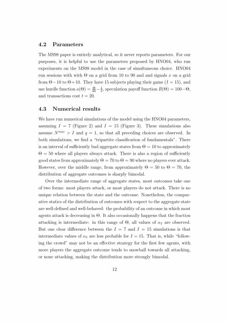
4.3 Numerical results

We have run numerical simulations of the model using the HNO04 parameters,

assuming I = 7 (Figure 2) and I = 15 (Figure 3). These simulations also

assume Nmax > I and q = 1, so that all preceding choices are observed. In

both simulations, we find a “tripartite classification of fundamentals”. There

is an interval of sufficiently bad aggregate states from Θ = 10 to approximately

Θ = 50 where all players always attack. There is also a region of sufficiently

good states from approximately Θ = 70 to Θ = 90 where no players ever attack.

However, over the middle range, from approximately Θ = 50 to Θ = 70, the

distribution of aggregate outcomes is sharply bimodal.

Over the intermediate range of aggregate states, most outcomes take one

of two forms: most players attack, or most players do not attack. There is no

unique relation between the state and the outcome. Nonetheless, the compar-

ative statics of the distribution of outcomes with respect to the aggregate state

are well-defined and well-behaved: the probability of an outcome in which most

agents attack is decreasing in Θ. It also occasionally happens that the fraction

attacking is intermediate: in this range of Θ, all values of αI are observed.

But one clear difference between the I = 7 and I = 15 simulations is that

intermediate values of αI are less probable for I = 15. That is, while “follow-

ing the crowd” may not be an effective strategy for the first few agents, with

more players the aggregate outcome tends to snowball towards all attacking,

or none attacking, making the distribution more strongly bimodal.

12

5 Experimental results

Our first experimental sessions had eight participants. They interacted via a

computer network, using z-Tree software (Fischbacher 1999). The participants

played nine rounds, and in each round they played our game eight times (in

parallel) so that we have 72 observations of the game per session. The play

passes through a series of decision steps, in each of which a participant makes

(at most) one choice. When a participant is required to make a choice, the

computer screen displays their information set to them. Specifically, they see

their signal x and their observations of the behavior of previous players: the

total number of observations n, the number attacking, m, and the number not

attacking, n − m. In some sessions, they know their position in the sequence,

because they have one choice in each decision step (so they know that they are

first in one sequence, second in another, etc.) In other sessions, we made the

number of decision steps substantially larger than the number of players, and

made some sequences starting later than others, so that players could not infer

their position from the timing of their choice. However, we have not noticed

any differences between the sessions in which position was or was not known.

We assume that Θ lies in a grid from 15 to 85, and that x is drawn from a

grid between Θ− 15 and Θ + 15. We imposed the speculation payoff function

R(Θ) = 100−Θ, hurdle function a(Θ) = Θ40− 3

4, and transactions cost t = 30.5

Figures 4 and 5 show the results of the first and fourth sessions, which

imposed q = 0.75 and q = 0, respectively. Both figures plot the contour

lines of the conditional distribution p(α8|θ) calculated numerically from the

theoretical model. The actual observations from the experiment are plotted as

stars, superimposed on the theoretical predictions. The data shown correspond

5HNO04 find subjects understand the game better if the meaning of the aggregate stateis reversed so that a′ < 0 and R′ > 0. Therefore they state the model in terms of thetransformed state variable Y ≡ Θ − 100. Also, they write the hurdle function as a numberof players rather than as a fraction. We follow their conventions. So when describing thegame to subjects, we state that the hurdle function is Ia(Y ) = 8( 100−Y

40− 3/4) = 14− 0.2Y

and that the payoff is R(Y ) = Y . We give a neutral description of the game, calling thechoices A and B, and making no reference to currency speculation.

13

to the last six of the nine rounds played, in order to remove any transitional

dynamics resulting from learning.6

In Figure 4, with a seventy-five percent probability of observing each previ-

ous player’s choice, players are able to coordinate strongly: the large majority

of outcomes have 0 or 1 or 8 attackers. An informal eyeball analysis of the

graph appears to reveal a tripartite classification of aggregate states. For low

θ, almost everyone attacks, and for high θ almost no one attacks. But there is

not an intermediate range with intermediate numbers attacking; even between

θ = 45 and θ = 55, which is approximately where the transition occurs, most

observations take extreme values of α. These include one history with θ = 45

and zero attackers, and another with θ = 51 and eight attackers. These ob-

servations appear to represent herding in the “wrong” direction, since overall

a higher θ corresponds to less attacks.

The experimental outcome also looks quantitatively quite consistent with

the theory. The contour lines show that there is a region of bimodality of

outcomes from approximately θ = 35 to θ = 64. But very low probability

events are not likely to have been picked up by our relatively small sample of

experimental points, so it may be more interesting to note that the interval

where there is more than a 30% chance of 0 attackers, and also more than a

30% chance of 8 attackers, is from θ = 45 to θ = 51. This is almost exactly the

same interval of θ where we actually observed herding to the wrong outcome.

The results of session 4, in which no previous actions are observed, so that

choice is effectively simultaneous, are shown in Figure 5. Unlike the previous

graph, theory predicts a unimodal distribution. The experiment reveals that

from θ = 35 to θ = 65, the fraction attacking gradually, smoothly, and almost

linearly decreases from one to zero. Thus the experimental distribution is

always clearly unimodal conditional on θ, and it is close to the distribution

implied by theory.

6Our impression is that players are initially somewhat predisposed to follow their ownsignals, but learn to follow others more over the first few rounds. But these learning effectsappear small: the graphs are quite similar when we include all rounds.

14

Of course, in both sessions 1 and 4, some experimental observations are well

outside the range predicted by the theoretical model. But given that the model

makes no allowance at all for human error, the fit is remarkably good. We now

go on to consider the 14 sessions that we have run so far, with 8 or 12 players,

to see how these results hold up. We have varied the probability of observing

previous actions of q = 0, q = 0.5, q = 0.75, and q = 1. We have allowed

for idiosyncratic signal ranges of θ ± 8 and θ ± 15. We have also compared

sessions in which players were informed of their position in the sequence, and

sessions where they could only deduce their position from their observations

of others. To summarize the different results obtained, we now estimate the

policy functions used in each session, and compare their implications. in

5.1 Estimating the policy function

A glance at Figures 4 and 5 suggests that the distribution of aggregate out-

comes implied by this game differs greatly depending on whether or not pre-

vious actions are observed. But it is hard to draw strong conclusions from

these figures because of the relatively small number of observations of indi-

vidual behavior— and the even smaller number of observations of aggregate

behavior— in each experimental session. Therefore, we next estimate the pol-

icy function used by our experimental subjects. We can use the estimated

policy function to calculate the distribution of aggregate outcomes associated

with each experimental session, thus obtaining a clearer, more quantitative

understanding of the differences in behavior across sessions.

In our theoretical model, players attack if and only if their signal exceeds

a threshold τ(n, m). Obviously, in the laboratory, play will be more random

than this. Thus we model our experimental subjects’ probability of attacking,

conditional on their information sets, by the following logistic function:

Probability of attacking:

prob(ηi = 1|xi, ni, mi) =1

1 + exp{γ(ni)[δ(ni) − xi − ξ(ni)(mi/ni − 0.5)]}(10)

15

In this formula, the probability of attacking, conditional on the information set

(xi, ni, mi), is a number between 0 and 1. This probability depends on three

parameters, γ(n), δ(n), and ξ(n), which may in general vary with the number

of observations n. The formula is written so that the estimates of γ(n), δ(n),

and ξ(n) ought to be positive. As long as γ is positive, the probability of

attacking is an increasing function of the signal x.

The parameters in the formula have straightforward interpretations. Pa-

rameter δ can be seen as an unconditional threshold signal. That is, if the

observations of other actions are uninformative (mi/ni = 0.5), then the player

attacks with probability 0.5 when she observes the signal xi = δ(ni).7 When

observations of other actions are informative (mi/ni 6= 0.5), then we can in-

terpret δ(n) − ξ(n)(mi/ni − 0.5) as the conditional threshold signal at which

the probability of attacking is one half. Note that if ξ is positive, then the

threshold signal for attacking is lower when a higher proportion of attacks is

observed. Finally, parameter γ(n) indexes the precision of individual behavior.

If γ(n) = 0, then behavior is always totally random; that is, the probability

of attacking is always 0.5. If γ(n) = ∞, then, as in our theoretical model,

there is no randomness in individual behavior, conditional on the individual

information set.

Using experimental data on signals xi, observations ni and mi, and deci-

sions ηi, we can estimate this policy function by maximum likelihood for each

experimental session. Once we have estimated the policy function, we can

then calculate the implied distribution of aggregate outcomes P (αI, Θ). We

can also use the estimated policy function to simulate additional experimental

sessions. By repeating our maximum likelihood estimation on these artificial

experimental data sets, we can obtain bootstrap estimates of the confidence

7The case ni = 0 is also an uninformative signal about others’ actions, so it should betreated analogously to the cases where mi/ni = 0.5. When the coefficients are allowedto vary with n, δ(0) and ξ(0) are not separately identified; in this case we preserve theinterpretation of δ(0) as an unconditional threshold signal by setting ξ(0) = 0. On the otherhand, when we do not allow the coefficients to vary with n, we preserve the interpretationof δ as an unconditional threshold signal by setting mi/ni ≡ 0.5 whenever ni = 0.

16

intervals on our parameter estimates. More importantly, we can likewise es-

timate confidence intervals for any statistics of the aggregate distribution P

that interest us.

Parameter estimates for each session are given in Tables 1-3. In order to

eliminate transitional dynamics in the policy coefficients caused by learning,

we have discarded the first two rounds of each session before estimating. The

coefficients γ, δ, and ξ are allowed to vary with n, but our relatively small num-

ber of data points (especially for high n) prevents us from allowing fully general

dependence on n. However, this appears not to be a problem. The likelihood

of our sample improves greatly if we allow ξ to change with n; in particular, we

estimate ξ02 ≡ ξ(n), n ∈ {0, 1, 2} separately from ξ37 ≡ ξ(n) n ∈ {3, 4, 5, 6, 7}.

Similarly, likelihood is improved by estimating δ02 ≡ δ(n), n ∈ {0, 1, 2} sep-

arately from δ37 ≡ δ(n), n ∈ {3, 4, 5, 6, 7}. We find allowing more general

dependence of the coefficients on n rarely yields significant improvement in

likelihood.8

The unconditional threshold signal δ is usually found to lie in the range from

45 to 50. Estimates of ξ(n) are robustly found to be larger when n is larger.

This makes sense: it means that subjects react more to the observed fraction

attacking if they have observed many actions. For example, the coefficient

estimates for session F3 imply that the difference between the threshold for

attacking when only attacks are observed, and when no attacks are observed, is

7.9 for n ≤ 2, but rises to 32.99 for n ≥ 3. In general, our estimates also show

that γ is somewhat larger for larger n. This means that subjects react more

strongly to deviations from their threshold signals when n is larger, suggesting

that they can be more decisive when they have better information.

We also report two statistics describing the distribution of aggregate out-

comes. We search for values of the aggregate state such that the conditional

distribution of αI , the aggregate fraction attacking, is bimodal. As our model

8Two times the log likelihood ratio between specifications is distributed as χ2(J), whereJ is the number of parameter restrictions between the two specifications; see Greene (1993),p. 365.

17

predicts, no bimodal region is detected for the sessions in which previous ac-

tions are unobserved, and generally the estimated bimodal region is larger

when more predecessors are observed. But unlike our theoretical model, in

which players act without error, only very mild bimodality is observed in the

experiment. The widest estimated region of bimodality is only 3.5 units wide,

and the bimodal regions are (individually) not statistically significant.

We also report the width of the region of fundamentals in which both the

lowest and the highest values of αI occur with at least 1% probability. Again,

as we would expect from our model, this region is wider when more previous

actions are observed. When no previous actions are observed, no aggregate

states are found in which both αI = 0 and αI = 1 occur. But when we

set q = 0.5, so that half of the preceding actions are observed, only one out

of 5 sessions fails to detect a region in which both extreme outcomes occur.

For the other four sessions with q=0.5, the width of the region of multiple

outcomes is estimated to be 1, 15.5, 8.5, or 13.5. For q = 0.75 and q = 1, we

always detect regions in which both extreme outcomes occur with at least 1%

probability. The estimated widths of the region of multiple outcomes for these

sessions is estimated at 14.5, 12.5, 10.5, 16.5, 15.0, 5.5, and 8.0; most of these

estimates are significant. Thus sessions with q ≥ 0.5 mostly appear to exhibit

a “tripartite classification” of aggregate fundamentals, with a middle region

where multiple outcomes can occur.

6 Conclusions

We have found that when previous actions are unobserved, there is a clearly

defined functional relationship (in spite of a small amount of random noise)

that determines the fraction attacking in terms of the fundamental. This

result, illustrated in Figure 5, reproduces the earlier experimental results of

Heinemann et. al. (2002), and is also consistent with the evidence of Cabrales

et. al. (2002); both papers found a unique relation between fundamentals and

outcomes in games with a small amount of imperfect information.

18

This is consistent with the global games literature’s claim that aggregate

outcomes are uniquely determined in games with a small amount of imperfect

information. Nonetheless, the results of Heinemann et. al. (2002) and Cabrales

et. al. (2002) are inconsistent with the global games results in an important

way: no experimental paper up to now has found an important difference be-

tween games with full information and games with a small amount of imperfect

information. Perhaps this should not be surprising, since the theoretical claim

that full-information and slightly imperfect information contexts differ sharply

rests on complicated multi-step iterated dominance calculations which exper-

imental subjects are probably unable to perform.

What the present paper adds to this experimental literature is that it shows

that there is a big difference between coordination games with simultaneous

and sequential choice. Our theoretical model of herding under incomplete

information, like the full-information multiple-equilibrium model of Obstfeld

(1996), exhibits three regions of aggregate behavior: always attack, never

attack, and (in a middle interval of fundamentals) multiplicity of aggregate

outcomes. These three regions occur in our experimental results, as long as

previous actions are observed with sufficiently high probability. In fact, when

we plot our experimental results against our theoretical predictions, the fit

appears remarkably good.

The only obvious inconsistency between our theory and our experimental

data is that the theoretical model predicts that outcomes should be sharply

bimodal in the region of multiplicity, whereas in our experimental results out-

comes are almost uniformly spread out from αI = 0 to αI = 1 in the region

of multiplicity. What appears to be occurring is that the aggregate outcome

converges very slowly away from unstable intermediate values of α to the sta-

ble extremes. If so, then this is consistent with results of Vives (1993) and

Chamley (2002) showing that herding models converge slowly.

However, the wide distribution of aggregate outcomes observed in the in-

terval of multiplicity does not detract from our main point: the aggregate

outcome is unpredictable over some intermediate range of fundamentals. Only

19

the probability distribution over aggregate outcomes can be predicted by the-

ory; the outcome itself cannot. In future work we would like to explore versions

of our game (such as logit equilibrium) that explicitly take into account ex-

perimental subjects’ tendency to make mistakes, in order to find a theoretical

model that attains even closer quantitative agreement with the data than we

already have.

References

Anderson, Lisa R., and Charles A. Holt (1997), “Informational Cascades inthe Laboratory.” A.E.R. 87 (5), pp. 847-62.

Anderson, Lisa R., and Charles A. Holt (1998), “Informational Cascade Ex-periments.” In Handbook of Results in Experimental Economics, CharlesPlott, ed., forthcoming 2004, Elsevier Science Ltd.

Banerjee, Abhijit (1992), “A Simple Model of Herd Behavior.” Q.J.E. 107 (3),pp. 797-818.

Bikhchandani, Sushil; David Hirshliefer, and Ivo Welch (1992), “A Theory ofFads, Fashion, Custom, and Cultural Change as Informational Cascades.”J.P.E. 100 (5), pp. 992-1026.

Bikhchandani, Sushil; David Hirshliefer, and Ivo Welch (1996), “InformationalCascades and Rational Herding: An Annotated Bibliography.” Availableat: http://welch.som.yale.edu/cascades/

Bikhchandani, Sushil; David Hirshliefer, and Ivo Welch (1998), “Learning fromthe Behavior of Others: Conformity, Fads, and Informational Cascades.”J.E.P. 12 (3) pp. 151-70.

Cabrales, Antonio; Rosemarie Nagel, and Roc Armenter (2002), “EquilibriumSelection through Incomplete Information in Coordination Games: an Ex-perimental Study.” Univ. Pompeu Fabra Economics Working paper #601.

Carlsson, Hans and Eric van Damme (1993), “Global Games and EquilibriumSelection.” Econometrica 61 pp. 989-1018.

Chamley, Christophe (1999), “Coordinating Regime Switches.” Q.J.E. 114(3), pp. 869-905.

Chamley, Christophe (2003A), “Dynamic Speculative Attacks.” A.E.R.

Chamley, Christophe (2003B), Rational Herds: Economic Models of SocialLearning, Cambridge University Press.

20

Chari, V.V., and Patrick Kehoe (2003), “Financial Crises as Herds: Overturn-ing the Critiques.” NBER Working Paper #9658.

Ciccone, Antonio, and James Costain (2001), “On Payoff Heterogeneity inGames with Strategic Complementarities.” Univ. Pompeu Fabra EconomicsWorking Paper #546.

Costain, James (2003), “A Herding Perspective on Global Games and Multi-plicity.” Univ. Carlos III Economics Working Paper # 03-29 (08).

Evans, George W., and Seppo Honkapohja (2001), Learning and Expectationsin Macroeconomics, Princeton University Press.

Fischbacher, Urs (1999), “z-Tree: Zurich Toolbox for Readymade EconomicExperiments— Experimenter’s Manual.” Working paper #21, Institute forEmpirical Research in Economics, University of Zurich. Additional infor-mation available at http://www.iew.unizh.ch/ztree.

Frankel, David M., Stephen Morris, and Ady Pauzner (2003), “EquilibriumSelection in Global Games with Strategic Complementarities.” J.E.T. 108,pp. 1-44.

Heinemann, Frank; Rosemarie Nagel; and Peter Ockenfels (2004), “The Theoryof Global Games on Test: Experimental Analysis of Coordination Gameswith Public and Private Information.” Econometrica 72 (5), pp. 1583-99.

Hellwig, Christian (2002), “Public Information, Private Information, and theMultiplicity of Equilibria in Coordination Games.” J.E.T. (107), pp. 191-222.

Holt survey paper

Kubler, Dorothea, and Georg Weizsacker (2004), “Limited Depth of Reasoningand Failure of Cascade Formation in the Laboratory.” Review of EconomicStudies 71, pp. 425-42.

Morris, Stephen, (2000), “Contagion.” R.E.Stud. 67, pp. 57-78.

Morris, Stephen, and Atsushi Kajii (1997), “The Robustness of Equilibriumto Incomplete Information.” Econometrica 65, pp. 1283-1309.

Morris, Stephen, and Hyun Song Shin (1998), “Unique Equilibrium in a Modelof Self-Fulfilling Currency Attacks.” A.E.R. 88 (3), pp. 587-97.

Morris, Stephen, and Hyun Song Shin (2003), “Heterogeneity and Uniquenessin Interaction Games.” Cowles Foundation Discussion Paper #1402, YaleUniv.

Obstfeld, Maurice (1996), “Models of Currency Crises with Self-Fulfilling Fea-tures.” E.E.R. 40 (3-5), pp. 1037-47.

Tarashev (2001)

Woodford, Michael (1990), “Learning to Believe in Sunspots.” Econometrica,58 (2), pp. 277-307.

21

Appendix A: Proofs

Appendix B: Simulation details

For numerical and experimental purposes, we assumed that the distributions

G(Θ) and F (x|Θ) place positive probability only on a discrete grid; let g(Θ) be

the probabilities associated with the grid points of the aggregate state. For a

given state Θ, if the first player uses strategy τ , then she will attack (implying

η1 = α1 = 1) with probability F (τ(0, 0)|Θ), since n = m = 0 for the first agent.

Starting here, we can calculate the probability of any fraction of attackers αi

up to and including individual i, conditional on some aggregate state Θ:

prob(αi = α|i, Θ, τ) for any α ∈ Ji

These probabilities can be calculated recursively, using the functions Ti:

prob(αi = α|i, Θ, τ) = prob(

αi−1 =iα

i − 1|i − 1, Θ, τ

) [

1 − Ti

(

iα

i − 1, Θ, τ

)]

+ prob(

αi−1 =iα − 1

i − 1|i − 1, Θ, τ

)

Ti

(

iα − 1

i − 1, Θ, τ

)

Next we can easily calculate the joint probability

prob(αi−1, Θ, i, n, m|τ) =

prob(αi−1|i − 1, Θ, τ)prob(i)prob(n|i)prob(m|n, αi−1, i)prob(Θ)

This is the joint probability that the player is the ith in the sequence, that

the state is Θ, that the fraction of predecessors attacking is αi−1, and that she

observes n predecessors, of whom m attacked, given that all other agents are

playing strategy τ . All the probabilities in this product are known from our de-

scription of the model: prob(i) = 1/I, prob(n|i) = Ni(n), prob(m|n, αi−1, i) =

Mi(m|n, αi−1), and prob(Θ) = g(Θ).

Now if trader i plays ηi = 1, then αi = ((i − 1)αi−1 + 1)/i ∈ {1i, 2

i, . . . , 1}.

Thus for αi = ((i − 1)αi−1 + 1)/i, we have

prob(αi, Θ, i, n, m|τ, ηi = 1) = prob(αi−1, Θ, i, n, m|τ)

22

From here, we go on updating, assuming that other agents play strategy

τ , to calculate probability distributions over αj for j > i. In the end, we need

the probabilities over αI , the aggregate fraction attacking; in particular, we

must know

prob(αI , Θ, i, n, m|τ, ηi = 1)

which is the joint probability of the event in which the aggregate outcome is

(αI , Θ), the player is the ith individual, and the player observes n predecessors

of whom m attack, given that others play strategy τ and the individual plays

ηi = 1. This can be calculated by updating with Ti, as we did before. For any

j > i and αj ∈ {1j, 2

j, . . . , 1},

prob(αj, Θ, i, n, m|τ, ηi = 1) = prob(

αj−1 =iαj

i − 1, Θ, i, n, m|τ, ηi = 1

) [

1 − Tj

(

iαj

i − 1, Θ, τ

)]

+ prob(

αj−1 =iαj − 1

i − 1, Θ, i, n, m|τ, ηi = 1

)

Tj

(

iαj − 1

i − 1, Θ, τ

)

Next, for any signal x, we can multiply by prob(x|Θ) to calculate

prob(αI , Θ, i, n, m, x|τ, ηi = 1)

which is the player’s distribution over the aggregate outcome conditional on

his information set and his action (we only need this information for the case

ηi = 1, since if ηi = 0 then the payoff is zero regardless of the aggregate

outcome). This, at last, is the probability that enters into formula (9) from

which we calculate the conditional probability Π(αI , Θ|n, m, x, ηi = 1) that the

player must know in order to choose his optimal policy.

23

Table 1: Estimated policy functions.Width Width

Session I q ε Position γ02 γ37 δ ξ12 ξ37 bimodal regionknown? region all possible

F4 8 0 15 yes 0.2281 n.a. 53.23 n.a. n.a. 0 0(0.0214) (0.685) (0) (0)

F7 8 0.5 15 no 0.3756 0.4354 41.19 3.707 12.37 0 1.0(0.0825) (21.6) (0.607) (2.37) (5.56) (0) (1.44)

F5 8 0.5 15 yes 0.3019 0.1366 48.45 18.51 51.92 1.5 15.5(0.0524) (0.0562) (1.21) (3.35) (30.0) (1.88) (2.33)

M4 8 0.5 15 no 0.2451 0.2957 50.29 5.429 28.27 0 6.0(0.0375) (5.1*1012) (1.09) (3.11) (14.8) (0) (3.17)

M2 8 0.5 15 yes 0.2796 0.2476 51.43 8.97 35.90 0 8.5(0.0863) (14.9) (1.04) (2.81) (113) (0.559) (2.34)

F1 8 0.75 15 no 0.1912 0.1422 51.03 12.71 36.56 0 14.5(0.0406) (0.0481) (0.716) (3.30) (45.6) (1.80) (3.34)

F3 8 0.75 15 yes 0.2963 1.155 43.19 7.899 32.99 1.5 12.5(0.0768) (2.2*1013) (0.7058) (3.639) (6.192) (5.371) (2.821)

M3 8 0.75 15 no 0.3493 0.2194 46.00 10.61 23.54 0 10.5(0.191) (0.0888) (1.24) (4.07) (7.12) (0.638) (2.95)

M1 8 0.75 15 yes 0.1444 0.1802 48.98 22.87 28.71 2.5 16.5(0.0315) (0.0495) (1.19) (7.12) (19.7) (4.89) (5.11)

F2 8 1 15 yes 0.1602 0.1046 44.20 0.8077 46.49 3.0 15.0(0.0338) (0.0233) (1.25) (5.24) (16.0) (4.09) (2.95)

Bootstrap standard errors in parentheses.

Data of first two rounds of each session deleted to eliminate nonstationary behavior due to learning.

Coefficient δ assumed independent of n; γ is estimated separately for n ∈ {0, 1, 2} and n ∈ {3, 4, 5, 6, 7},

while ξ is estimated separately for n ∈ {1, 2} and n ∈ {3, 4, 5, 6, 7}.

Note: In bootsim.mat, coeffs are called MLE-original (using specification 3), and standard errors are called stderrBOOTVEC.

24


Session I q ε Position γ δ ξ12 ξ37 bimodal regionknown? region all possible

F4 8 0 15 yes 0.2281 53.23 n.a. n.a. 0 0(0.0214) (0.685) (0) (0)

F7 8 0.5 15 no 0.3875 41.22 3.571 13.14 0 1.5(0.0765) (0.633) (2.59) (5.53) (0) (1.60)

F5 8 0.5 15 yes 0.2450 48.48 20.11 34.81 0 13.5(0.0442) (1.18) (3.62) (195) (2.37) (2.92)

M4 8 0.5 15 no 0.2519 50.17 5.289 30.86 0 6.0(0.0391) (1.04) (3.34) (287) (0.224) (2.69)

M2 8 0.5 15 yes 0.2730 51.41 9.110 35.07 0 8.5(0.0753) (1.0568) (2.85) (13.0) (0) (2.60)

F1 8 0.75 15 no 0.1752 51.08 14.00 29.21 0 13.5(0.0333) (1.15) (4.69) (9.25) (4.19) (4.46)

F3 8 0.75 15 yes 0.3452 43.17 7.136 34.36 0 13.0(0.0663) (0.851) (2.99) (7.30) (2.74) (2.46)

M3 8 0.75 15 no 0.2855 45.82 11.63 19.61 0 9.0(0.101) (1.13) (4.64) (3.85) (0.919) (2.38)

M1 8 0.75 15 yes 0.1535 48.73 21.63 33.76 3.5 18.0(0.0259) (1.24) (6.06) (10.8) (5.17) (4.97)

F2 8 1 15 yes 0.1378 44.10 2.330 33.29 0.5 13.0(0.0195) (1.41) (5.89) (8.11) (3.57) (4.34)



Coefficients γ and δ assumed independent of n; ξ is estimated separately for n ∈ {1, 2} and n ∈ {3, 4, 5, 6, 7}.

Note: In bootsim.mat, coeffs are called MLE-original (using specification 3), and standard errors are called stderrBOOTVEC.

25


Session I q ε Position γ02 γ37 δ ξ12 ξ37 bimodal regionknown? region all possible

F9 8 0 8 yes 0.4712 n.a. 48.43 n.a. n.a. 0 0(0.105) (0.859) (0) (0)

F10 8 1 8 yes 0.9200 0.3488 43.53 4.799 12.67 0 5.5(1.5*1013) (0.373) (0.953) (4.0*1010) (6.67) (4.93) (2.42)

F6 12 0.5 15 yes 0.2847 0.07991 48.96 8.861 40.68 0 0(0.0663) (0.0209) (1.22) (2.14) (20.9) (0) (0.671)

F8 12 0.75 15 yes 0.4188 0.1153 49.60 12.28 50.84 1.0 8.0(0.162) (0.0393) (1.29) (2.62) (22.7) (2.36) (2.30)

M5 16 0.5 15 yes



Coefficient δ assumed independent of n; γ is estimated separately for n ∈ {0, 1, 2} and n ∈ {3, 4, 5, 6, 7},

while ξ is estimated separately for n ∈ {1, 2} and n ∈ {3, 4, 5, 6, 7}.

Note: In bootsim.mat, coeffs are called MLE-original (from specification 3), and standard errors are called stderrBOOTVEC.

26

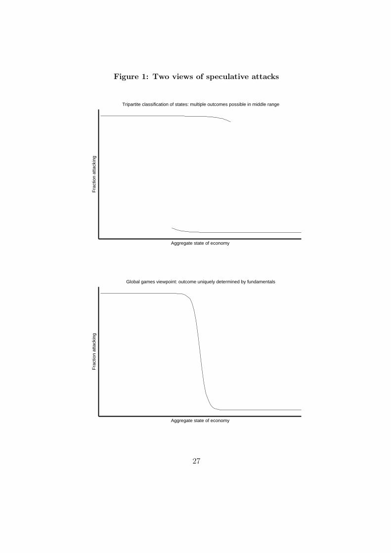
Figure 1: Two views of speculative attacks

Global games viewpoint: outcome uniquely determined by fundamentals

Aggregate state of economy

Fra

ctio

n at

tack

ing

Tripartite classification of states: multiple outcomes possible in middle range

Aggregate state of economy

Fra

ctio

n at

tack

ing

27

Figure 2: Conditional probabilities p over outcomes: I = 7

020

4060

80100

0

2

4

6

80

0.2

0.4

0.6

0.8

1

Aggregate stateNumber attacking

Pro

babi

lity

of h

isto

ry

28

Figure 3: Conditional probabilities p over outcomes: I = 15

020

4060

80100

0

5

10

150

0.2

0.4

0.6

0.8

1

Aggregate stateNumber attacking

Pro

babi

lity

of h

isto

ry

29

Figure 4: Theoretical and experimental distribution of outcomes:

Session 1

20 30 40 50 60 70 800

1

2

3

4

5

6

7

8

Aggregate state

Num

ber

atta

ckin

g

Probability contours: 0.01, 0.02, 0.04, 0.08, 0.16, 0.32, 0.64

30

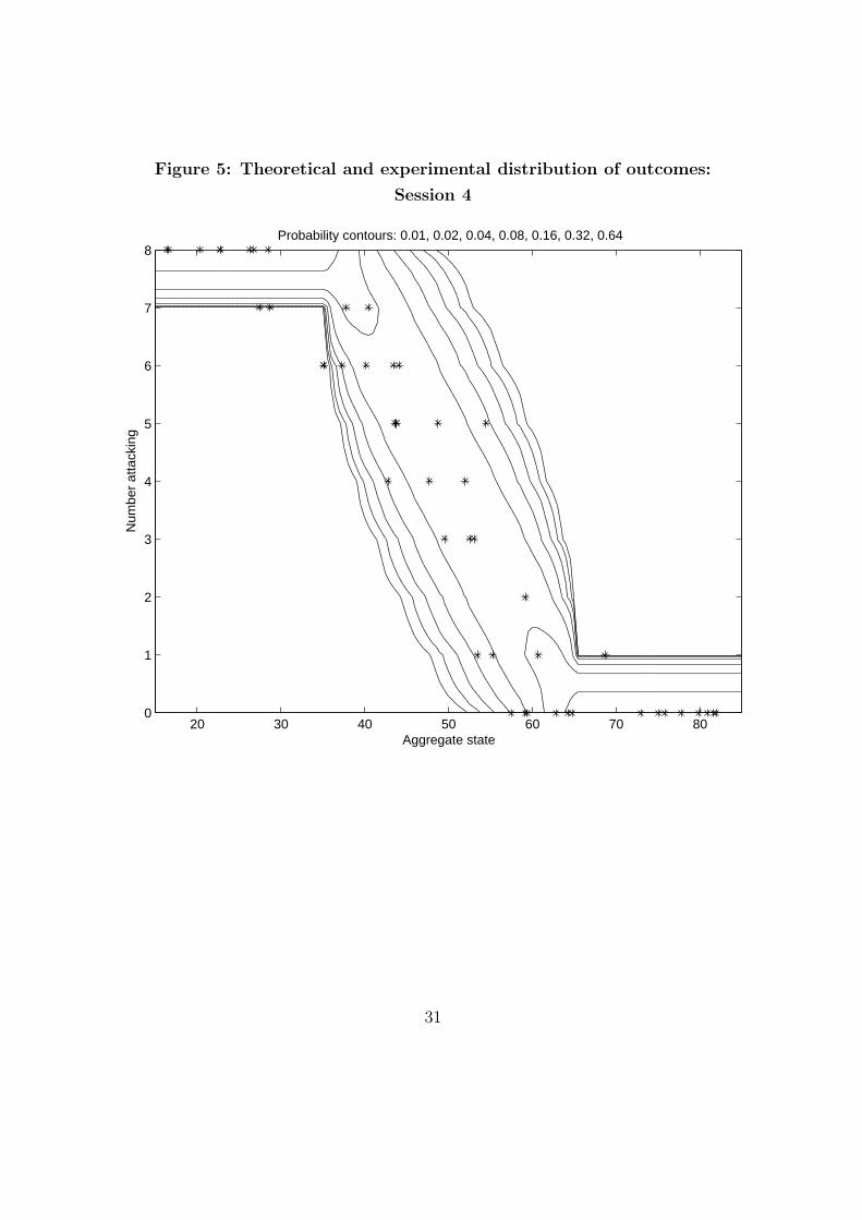
Figure 5: Theoretical and experimental distribution of outcomes:

Session 4

20 30 40 50 60 70 800

1

2

3

4

5

6

7

8

Aggregate state

Num

ber

atta

ckin

g

Probability contours: 0.01, 0.02, 0.04, 0.08, 0.16, 0.32, 0.64

31

multiple outcomes of speculative behavior in theory and in ... · multiple outcomes of speculative...

Documents