Multiple Regression Analysis

Multiple regression uses many independentvariables to predict or explain the variationin a dependent variables

The basic multiple regression model is a first-order model, containing each predictorbut no nonlinear terms such as squared values.

In this model, each slope should be interpretedas a partial slope, the predicted effect of a one-change in a variable, holding all other variablesconstant.

Multiple Regression Analysis

Estimating Equation Describing Relationshipamong Three Variables

2211 XbXbaY

nnXbXbXbaY .....ˆ2211

Estimating Equation Describing Relationshipamong n Variables

Multiple Regression Analysis – Example File: PPT_MultRegr

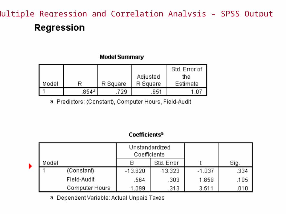
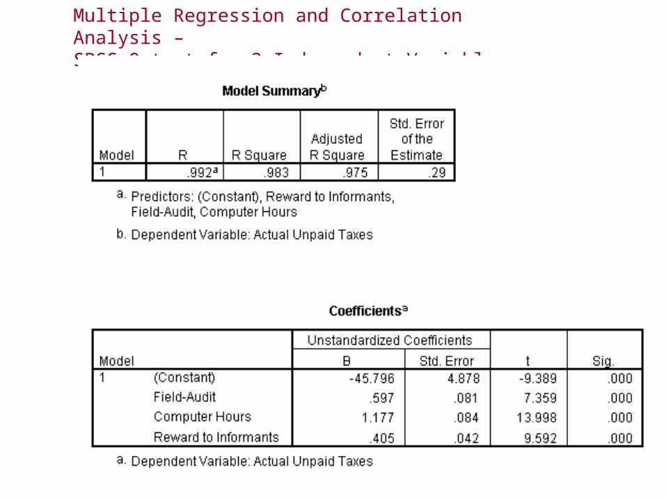
The department is interested to know whether the amount of field audits and computer hours spent on tracking have yielded any results. Further the department has introduced the reward system for tracking the culprits. The data on actual unpaid taxes for ten cases is considered for analysis. Initially the regression of Actual Unpaid Taxes(Y) on Field Audits(X1) and Computer Hours(X2) was carried out and as a next step the Reward to Informants(X3) was also considered as a variable and analyzed. The analysis yielded the following SPSS outputs.

Multiple Regression and Correlation Analysis – Excel Output

SUMMARY OUTPUT

Regression Statistics

Multiple R 0.85377

R Square 0.72892322

Adjusted R Square 0.65147271

Standard Error 1.07063884

Observations 10

ANOVA

  df SS MS FSignificance

F

Regression 2 21.57612732 10.78806 9.411471 0.010371059

Residual 7 8.023872679 1.146268

Total 9 29.6     

  CoefficientsStandard

Error t Stat P-value Lower 95%Upper 95% Lower 95.0% Upper 95.0%

Intercept -13.819629 13.3232999 -1.03725 0.334115 -45.32422668 17.68497 -45.324227 17.68496939

X Variable 1 0.56366048 0.303273881 1.858586 0.10543 -0.153468296 1.280789 -0.1534683 1.280789251

X Variable 2 1.0994695 0.313139013 3.511123 0.009844 0.359013391 1.839926 0.35901339 1.839925601

Multiple Regression and Correlation Analysis – SPSS Output

SUMMARY OUTPUT

Regression StatisticsMultiple R 0.9916677R Square 0.9834049Adjusted R Square 0.9751073Standard Error 0.2861281

Observations 10

ANOVA  df SS MS F Significance F

Regression 3 29.1087841 9.702928 118.51727 9.93505E-06Residual 6 0.491215904 0.081869

Total 9 29.6     

  Coefficients Standard Error t Stat P-value Lower 95%Upper 95%

Intercept -45.796348 4.877650787 -9.38902 8.288E-05 -57.73152916 --3.8612X Variable 1 0.5969718 0.081124288 7.358731 0.0003225 0.398467818 0.795476X Variable 2 1.1768377 0.084074178 13.99761 8.29E-06 0.971115623 1.38256

X Variable 3 0.4051086 0.042233591 9.592096 7.341E-05 0.301766772 0.508451

Multiple Regression and Correlation Analysis – Excel Output for 3 Independent Variables

Multiple Regression and Correlation Analysis – SPSS Output for 3 Independent Variables

Multiple Regression and Correlation Analysis

2211 XbXbaY

21 0991564082013 X.X..Y Using two independent variables :

321 40501771597079645 X.X.X..Y

Using three independent variables:

From the output, R2 = 0.983 98.3% of the variation in actual unpaid taxes is

explained by the three independent variables. 1.7% remains unexplained.

Coefficient of Determination

Multiple Regression and Correlation Analysis

Making inferences about Population Parameters

1. Inferences about an individual slope or whether a variable is significant

2. Regression as a whole

Multiple Regression and Correlation Analysis

Inferences about the Regression as a Whole

0321 BBB:H o

01 iBatleastone:H

Multiple Regression and Correlation Analysis

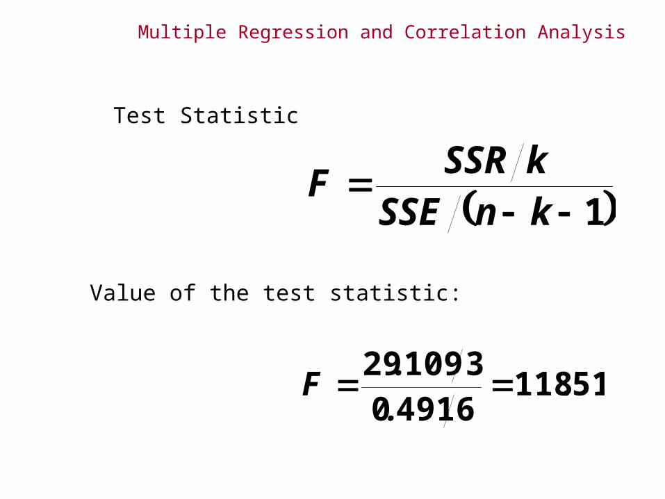
Test Statistic

1

knSSEkSSR

F

Value of the test statistic:

5111864910310929

...

F

Multiple Regression and Correlation Analysis

Multiple Regression and Correlation Analysis

Test of whether a variable is significant.

Test whether reward to informants is a significantexplanatory variable.

030 B:H

031 B:H

Multiple Regression and Correlation Analysis

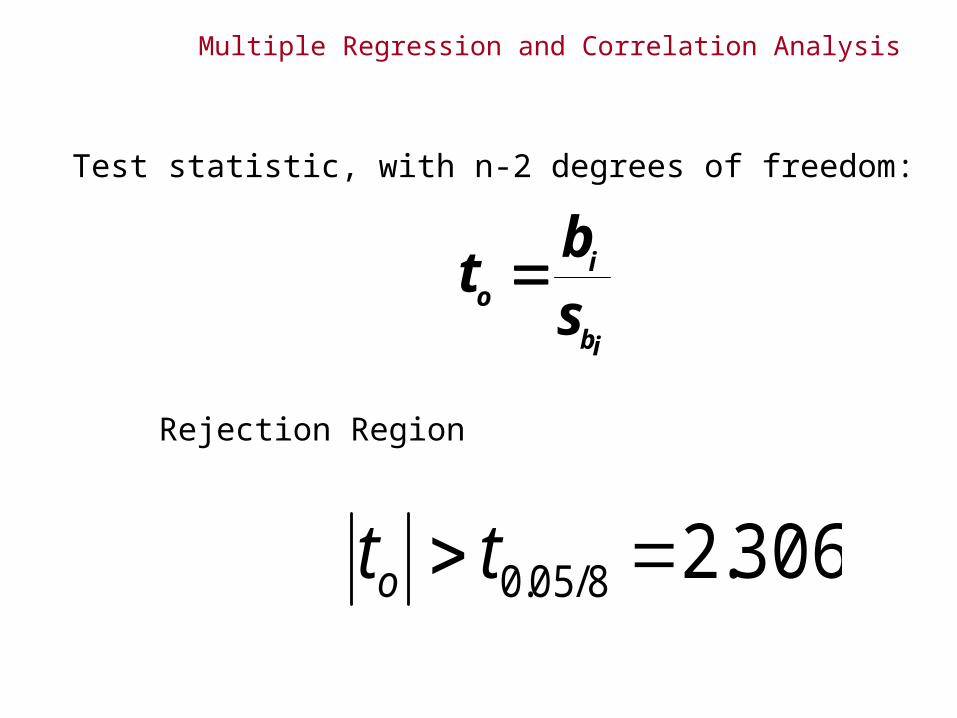
Test statistic, with n-2 degrees of freedom:

ib

io sb

t

Rejection Region

306.28/05.0 tto

Multiple Regression and Correlation Analysis

Value of the test statistic:

ib

io s

bt 64299

04204050

...

to

Conclusion:

The standardized regression coefficientis 9.6429 which is outside the acceptanceregion. Therefore we will reject the null hypothesis. The reward to informants is a significant explanatory variable.

b0 = - 45.796. This is the intercept, the value

of y when all the variables take the value

zero. Since the data range of all the

independent variables do not cover the value

zero, do not interpret the intercept.

b1 = 0.597. In this model, for each additional

field audit, the actual unpaid taxes increases

on average by .597% (assuming the other

variables are held constant).

Interpreting the Coefficients

Where to locate a new motor inn?– La Quinta Motor Inns is planning an

expansion.– Management wishes to predict which sites are

likely to be profitable.– Several areas where predictors of profitability

can be identified are:• Competition• Market awareness• Demand generators• Demographics• Physical quality

Estimating the Coefficients and Assessing the Model, Another Example

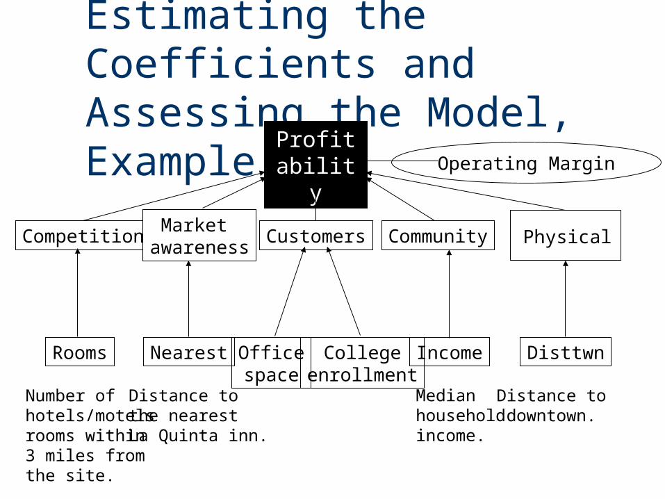
Estimating the Coefficients and Assessing the Model, Example

Profitability

Competition Market awareness Customers Community Physical

Operating Margin

Rooms Nearest Officespace

Collegeenrollment

Income Disttwn

Distance to downtown.

Medianhouseholdincome.

Distance tothe nearestLa Quinta inn.

Number of hotels/motelsrooms within 3 miles from the site.

Data were collected from randomly selected 100 inns that belong to La Quinta, and ran for the following suggested model (Multiple Regr_Margin.sav):

Margin = Rooms NearestOfficeCollege + 5Income + 6Disttwn

Estimating the Coefficients and Assessing the Model, Example

Margin Number Nearest Office Space Enrollment Income Distance55.5 3203 4.2 549 8 37 2.733.8 2810 2.8 496 17.5 35 14.449 2890 2.4 254 20 35 2.6

31.9 3422 3.3 434 15.5 38 12.157.4 2687 0.9 678 15.5 42 6.949 3759 2.9 635 19 33 10.8

This is the sample regression equation (sometimes called the prediction equation)This is the sample regression equation (sometimes called the prediction equation)

Regression Analysis, SPSS Output

Margin = 38.139 - 0.008Number +1.646Nearest + 0.020Office Space +0.212Enrollment + 0.413Income - 0.225Distance

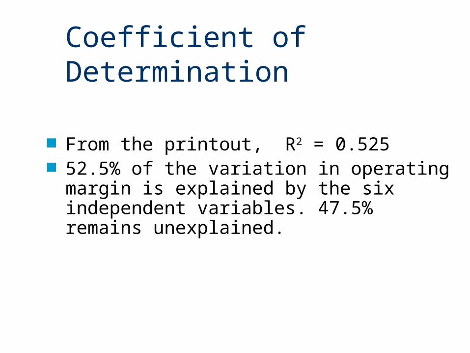
From the printout, R2 = 0.525 52.5% of the variation in operating margin is

explained by the six independent variables. 47.5% remains unexplained.

Coefficient of Determination

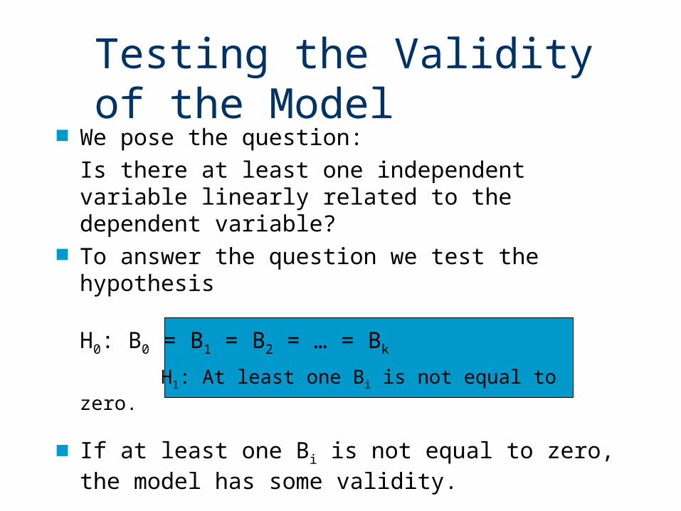
We pose the question:

Is there at least one independent variable linearly related to the dependent variable?

To answer the question we test the hypothesis

H0: B0 = B1 = B2 = … = Bk

H1: At least one Bi is not equal to zero.

If at least one Bi is not equal to zero, the model has some validity.

Testing the Validity of the Model

The hypotheses are tested by an ANOVA procedure ( the SPSS output)

Testing the Validity of the La Quinta Inns Regression Model

MSE=SSE/(n-k-1)

MSR=SSR/k

MSR/MSE

SSE

SSR

k =n–k–1 = n-1 =

ANOVAdf SS MS F Significance F

Regression 6 3123.8 520.6 17.14 0.0000Residual 93 2825.6 30.4Total 99 5949.5

F,k,n-k-1 = F0.05,6,100-6-1=2.17F = 17.14 > 2.17

Also, the p-value (Significance F) = 0.0000Reject the null hypothesis.

Testing the Validity of the La Quinta Inns Regression Model

ANOVAdf SS MS F Significance F

Regression 6 3123.8 520.6 17.14 0.0000Residual 93 2825.6 30.4Total 99 5949.5

Conclusion: There is sufficient evidence to reject the null hypothesis in favor of the alternative hypothesis. At least one of the i is not equal to zero. Thus, at least one independent variable is linearly related to y. This linear regression model is valid

Conclusion: There is sufficient evidence to reject the null hypothesis in favor of the alternative hypothesis. At least one of the i is not equal to zero. Thus, at least one independent variable is linearly related to y. This linear regression model is valid

b0 = 38.139. This is the intercept, the value of y

when all the variables take the value zero.

Since the data range of all the independent

variables do not cover the value zero, do not

interpret the intercept.

b1 = – 0.008. In this model, for each additional

room within 3 mile of the La Quinta inn, the

operating margin decreases on average

by .008% (assuming the other variables are

held constant).

Interpreting the Coefficients

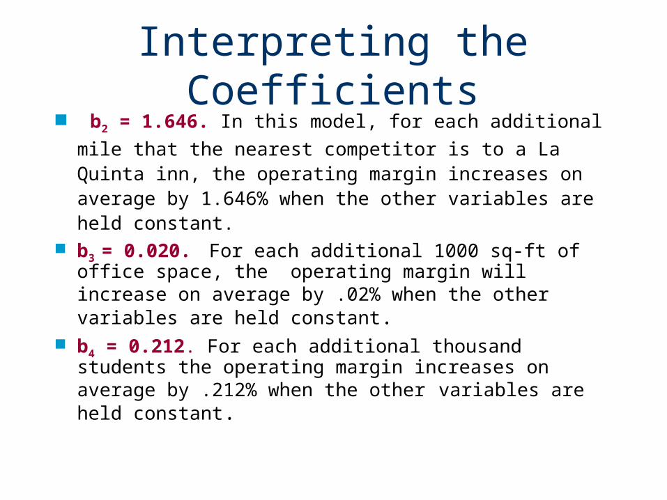
b2 = 1.646. In this model, for each additional mile

that the nearest competitor is to a La Quinta inn, the operating margin increases on average by 1.646% when the other variables are held constant.

b3 = 0.020. For each additional 1000 sq-ft of office space, the operating margin will increase on average by .02% when the other variables are held constant.

b4 = 0.212. For each additional thousand students the operating margin increases on average by .212% when the other variables are held constant.

Interpreting the Coefficients

b5 = 0.413. For additional $1000 increase in median household income, the operating margin increases on average by .413%, when the other variables remain constant.

b6 = -0.225. For each additional mile to the

downtown center, the operating margin

decreases on average by .225% when the other

variables are held constant.

Interpreting the Coefficients

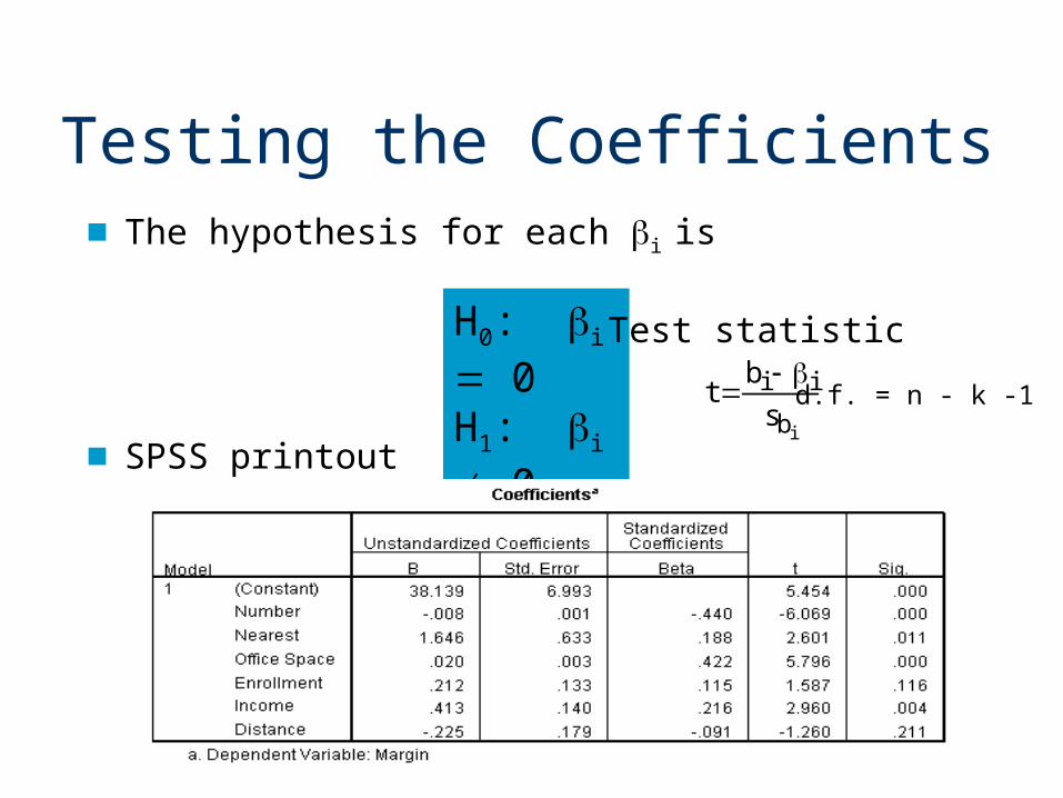
The hypothesis for each i is

SPSS printout

H0: i 0H1: i 0 d.f. = n - k -1

Test statistic

ib

iis

bt

Testing the Coefficients

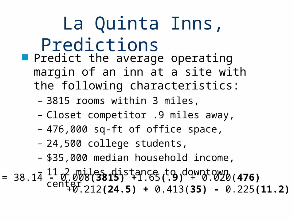
Predict the average operating margin of an inn at a site with the following characteristics:– 3815 rooms within 3 miles,– Closet competitor .9 miles away,– 476,000 sq-ft of office space,– 24,500 college students,– $35,000 median household income,– 11.2 miles distance to downtown center.

MARGIN = 38.14 - 0.008(3815) +1.65(.9) + 0.020(476) +0.212(24.5) + 0.413(35) - 0.225(11.2) = 37.1%

La Quinta Inns, Predictions