multiple-view tracing for haskell: a new hat

Kent Academic RepositoryFull text document (pdf)

Copyright & reuse

Content in the Kent Academic Repository is made available for research purposes. Unless otherwise stated all

content is protected by copyright and in the absence of an open licence (eg Creative Commons), permissions

for further reuse of content should be sought from the publisher, author or other copyright holder.

Versions of research

The version in the Kent Academic Repository may differ from the final published version.

Users are advised to check http://kar.kent.ac.uk for the status of the paper. Users should always cite the

published version of record.

Enquiries

For any further enquiries regarding the licence status of this document, please contact:

[email protected]

If you believe this document infringes copyright then please contact the KAR admin team with the take-down

information provided at http://kar.kent.ac.uk/contact.html

Citation for published version

Wallace, Malcolm and Chitil, Olaf and Brehm, Thorsten and Runciman, Colin (2001) Multiple-ViewTracing for Haskell: a New Hat. In: 2001 ACM SIGPLAN Haskell Workshop.

DOI

Link to record in KAR

https://kar.kent.ac.uk/13566/

Document Version

UNSPECIFIED

Multiple-View Tracing for Haskell: a New Hat

Malcolm Wallace, Olaf Chitil, Thorsten Brehm and

Colin Runciman

University of York, UK{malcolm,olaf,thorsten,colin}@cs.york.ac.uk

Abstract

Different tracing systems for Haskell give different views of a program at work. Inpractice, several views are complementary and can productively be used together.Until now each system has generated its own trace, containing only the informationneeded for its particular view. Here we present the design of a trace that can serveseveral views. The trace is generated and written to file as the computation pro-ceeds. We have implemented both the generation of the trace and several differentviewers.

1 Introduction

Usually, a computation is treated as a black box that performs input andoutput actions, but whose internal workings are invisible. As programmers,however, we may want to look into the black box to understand how thedifferent parts of the program cause the computation to perform the observedactions. Often the computation does not perform the intended actions and wehave to determine which parts of the program cause the erroneous behaviour.Even if a program is correct, we may desire to understand its parts better byseeing “how it works”; especially when we have to modify a program that wedid not write ourselves. Also for teaching it is sometimes useful to “see” acomputation.

In [2] we compared the Haskell tracing systems Freja 1 [5,6] and HOOD 2

[3] with our Haskell tracer Hat 3 [9,10,11]. The main conclusion of our com-parison was that each system gives a unique view of a computation and theseviews are usefully complementary. In experiments, we discovered that afterusing one system to help track a bug to a certain point, users often wanted tochange to another system to continue the search, or to confirm their suspicions.

1 http://www.ida.liu.se/~henni2 http://www.haskell.org/hood3 http://www.cs.york.ac.uk/fp/hat

151

Wallace, Chitil, Brehm and Runciman

All three tracing systems take a two-phase approach to tracing: duringthe computation information describing the computation is collected in a datastructure, the trace. After termination of the computation the trace is viewed.An advantage of a trace as a concrete data structure is that it liberates theviewer from the time arrow of the computation. However, each system createsits own trace, containing only the information required for its particular view.We noted in [2] that Hat’s trace, called a Redex Trail, contains nearly allthe information contained in Freja’s trace. Hence we decided to extend theRedex Trail structure to the Augmented Redex Trail structure (ART). Withseparate tools we can view an ART trace in at least three different ways: ala Freja, a la Hat and a la HOOD. Whereas Freja, HOOD and the old Hatsystem generated their traces in main memory, the new Hat writes the ARTtrace to file as computation proceeds. Hat’s new architecture has the followingadvantages:

• As a stand-alone description of a computation, the ART trace serves as in-terface between trace generation and trace viewing. The two phases becomecompletely separate.

• A trace in file supports sequential access and forms of indexed search thatwere not feasible for heap-based traces.

• The ART trace clarifies the relationships between the different views of acomputation. It suggests ways for integrating different views and creatingnew views.

• The size of the trace is no longer bound by the size of the main memorybut only by the far larger size of the file store.

• The trace is no longer transient but can be archived for later viewing.

• Trace system developers only need to implement trace generation once forseveral views.

• The user only pays the cost of generating a trace once for several views.

In Section 2 we review the Redex Trail of the old Hat system, while Section3 briefly illustrates some alternative tracing views. In Section 4 we developin several steps the new Augmented Redex Trail structure. In Section 5 wedescribe how several tools for different views obtain their information fromthe ART trace. In Section 6 we outline the generation of the ART trace. InSection 7 we discuss ideas for future work. Section 8 concludes.

We have modified Hat to produce the ART trace and have implementednew tools for viewing the trace in the style of Freja and HOOD. The systemhas been publicly released as Hat 1.04.

2 The Redex Trail Model

Let us view a computation abstractly as a series of rewrite steps. Startingfrom a single expression (main), at each step a reducible expression (redex)

152


is replaced by another expression (its reduct), by instantiating the lhs ofan equation, and replacing it with the corresponding instance of the rhs.Eventually, only irreducible expressions (values) remain.

The original Redex Trail structure is a directed graph, recording copiesof all values and redexes, with a backward link from each reduct (and eachproper subexpression contained within it) to the parent redex that created it.

2.1 Example

oneTrue :: [Bool ] → Bool

oneTrue [] = False

oneTrue (x : xs) = xor x (oneTrue xs)

xor :: Bool → Bool → Bool

xor x True = not x

xor False = True

main = print (oneTrue [False, not True])

Fig. 1. Example program

The small example program shown in Figure 1 produces the Redex Trailillustrated in Figure 2. A subexpression with a different parent is representedas a box within a box. A solid arrow denotes the parent relationship. Ofcourse, the user is not expected to see and understand a complete graph ofthis nature. A tool called the Redex Trail viewer permits the whole graphto be explored interactively one expression at a time, as illustrated in thissnapshot:

• True

not False

xor False True

• xor (not True) False

▽ oneTrue []

▽ oneTrue (not True : [])

oneTrue (False : not True : [])

main

Each redex is shown on a separate line. The parent of an expression isshown below it. (Because parents are shown below their children in the viewer,we have drawn the full graph in Figure 2 similarly.) The parent of a whole

153


main

oneTrue [False, not True]

oneTrue [not True]

oneTrue []

xor (not True) False

xor False True

not False

True

Fig. 2. An example of a Redex Trail

redex starts in the same column, whereas the parent of a proper subexpressionis further indented. Underlining, and colouring if available, is used to show towhich subexpression a parent belongs.

2.2 Structure

Figure 3 formalises the Redex Trail structure as a set of concrete Haskelltypes. An App node represents a redex in the obvious way, with a trace for thefunction and separate traces for each argument. It also contains the parent

trace describing the redex that created it. Each function and argument islikewise of Trace type and therefore has its own, possibly different, parent. TheSrcPos type records the location in the source code of the relevant applicationsite on the rhs of a definition.

A Const node represents an irreducible value (an Atom), such as an integer,character, or a constructor or named function from the program, representedsimply as a string identifier. (In the latter case, a SrcPos is associated withthe identifier to record its static definition site.) A Const node also has a

154


data Trace = App { fun :: Trace, args :: [Trace], parent :: Trace, src :: SrcPos }

| Const { value :: Atom

, parent :: Trace, src :: SrcPos }| Root

data SrcPos = SrcPos { file :: FilePath

, line :: Int , column :: Int }| NoPos

data Atom = Id String SrcPos | IntVal Int | CharVal Char | ...

Fig. 3. The original Redex Trail structure.

parent redex and a SrcPos to indicate its dynamic origin. For instance, twouses of the function f in a computation may have different positions in thesource code, because they are introduced to the trace by rewriting differentredexes.

Finally, it is possible for a redex to have no parent, represented simply asRoot . This clearly occurs at the very start of the computation, namely for themain function. It also applies in the case of other top-level pattern-bindings(cafs).

3 Alternative Views

We would like to adapt the original Redex Trail structure to support additionalstyles of viewing, such as Algorithmic Debugging and Observations. So whatdo these views look like? And what information do they require from thetrace?

3.1 Algorithmic Debugging

Algorithmic Debugging is a well-known technique in declarative languages [8],implemented for a subset of Haskell by the Freja system [5]. The algorithmlocates an error in a program, given a user who can provide answers to asequence of questions. Each question concerns a reduction of a redex to aresult, presented as an equation. The user should answer yes if the equationis correct with respect to his intentions, and no otherwise. After some numberof questions, the system identifies an incorrect function definition.

Here is such a session for the example program of Figure 1. The symbol‘ ’ represents an expression that has never been evaluated and whose valuehence cannot have influenced the computation.

1> oneTrue (False:_:[]) = True (Y/?/N): n

2> oneTrue (_:[]) = True (Y/?/N): n

3> oneTrue [] = False (Y/?/N): y

4> xor _ False = True (Y/?/N): n

155


Error located!

Bug found in: xor _ False = True

Freja creates an Evaluation Dependency Tree (EDT) as its trace structure.Figure 4 shows the EDT for this example. Each node of the tree is a reduction.The tree is basically the derivation/proof tree for a call-by-value reduction withmiraculous stops where expressions are not needed for the result. The call-by-value structure ensures that the tree structure reflects the program structureand that arguments are maximally evaluated.

main ⇒ True

oneTrue [False, ] ⇒ True

oneTrue [ ] ⇒ True xor False True ⇒ True

oneTrue [] ⇒ True xor False ⇒ True not False ⇒ True

Fig. 4. An Evaluation Dependency Tree

The viewer dialogue walks the tree, presenting each node as a question –some answers permit some branches of the tree to be ignored.

To allow algorithmic debugging starting from a Redex Trail rather thanan EDT, we need to add the ability to extract redexes from deep within theTrail – for instance, the very first question is about the reduction of main,which lies at the farthest tip of the Redex Trail graph. Furthermore, we needto record dependency information in the opposite direction – the reduction ofan expression depended on what sub-reductions?

3.2 Observations

HOOD [3] allows observation of individual values within computations. Theprogrammer annotates the expression(s) of interest in the program source withthe combinator observe. For each annotation, HOOD records the value inall of its intermediate stages of evaluation, so that after termination of thecomputation the observed expression can be shown to exactly the degree towhich it was demanded.

By a few clever tricks, HOOD can record not only data values, but alsofunctional values, again only to the degree they are really used in the compu-tation. Thus a functional value is recorded as a bag of actual argument/result

156


data StoredEvent = Value { value :: String

, inside :: Ref , position :: Int }| Constr { name :: String , arity :: Int

, inside :: Ref , position :: Int }type Observation = Ref → StoredEvent

data ObservedValue = Value { value :: String }| Constr { name :: String

, arguments :: [ObservedValue] }

Fig. 5. The two HOOD observation structures. StoredEvents are recorded as asimple sequence during the computation, but the viewer must later traverse theStoredEvents to construct an ObservedValue that can be displayed.

mappings [4].

Here we illustrate the output when observing the functions oneTrue andxor in our example program. The symbol ‘ ’ again represents an unevaluatedexpression.

oneTrue (False:_:[]) = True

oneTrue (_:[]) = True

oneTrue [] = False

xor False True = True

xor _ False = True

The HOOD trace structure (sketched in Figure 5) is a sequence of individ-ual ‘events’. Every event represents the creation of a data value or constructor(in whnf) during the computation. It has a backwards link to identify the en-closing data structure of which it is a component, and the particular argumentposition it occupies. Each constructor also has a note of how many argument‘holes’ it can accept. A functional value is treated like a data constructor withtwo components, an argument and a result.

At viewing time, the HOOD viewer transforms the stored structure inter-nally by constructing forward links from each constructor to the final value ofeach of its components. This can be expensive for a large structure.

The most notable difference between these structures and the Redex Trailis that HOOD stores only irreducible values, not reducible expressions. An-other major difference is that HOOD records only individual annotated values,not a full trace of the whole computation.

In another paper at this workshop Reinke describes a graphical viewer forHOOD observations [7].

157


4 The Augmented Redex Trail Structure

The EDT structure used in Freja’s algorithmic debugging is very similar toa substructure of the Redex Trail, but with pointers reversed. Most of theinformation in HOOD’s Observations can be derived from either an EDT ora Redex Trail by searching through those structures for named values andsource positions. The Redex Trail lacks some small pieces of information thatwould permit the reconstruction of an EDT by the reversal of pointers. Thissame lack also prevents the reconstruction of Observations.

In this section we extend the original structure in stages to become theAugmented Redex Trail, or ART structure. 4

4.1 Linearisation and Explicit Sharing

The original Redex Trail is an ephemeral heap-based structure, but we wantto store the trace in a file so it is persistent, does not depend on connecting aviewer to a live program, and can be accessed many times by different tools.

The original Redex Trail type Trace (in Figure 3) is self-recursive, so toplace it in file requires the structure to be linearised. Linearisation gives twobenefits: we can write the trace into the file one node at a time; and we canaccess a part of the trace piecemeal without necessarily following all possiblepaths. In both cases, efficiency is important: when generating, sequentialwriting is best; when viewing, the viewer tool should need to read only asmall fragment of the whole structure.

Another benefit of linearising the structure is that it makes sharing ofnodes explicit. In the original graph model, sharing and cycles are implicitvia the self-recursive type, but in the new model this information is revealeddirectly to the viewing tool. There is a great deal of sharing in a trace of atypical program.

data Expr = App { fun :: Ref , args :: [Ref ], parent :: Ref , src :: SrcPos }

| Const { value :: Atom

, parent :: Ref , src :: SrcPos }| Root

type Trace = Ref → Expr

data Ref = NoRef | Ref FilePos deriving Eq

Fig. 6. The linearised Redex Trail structure.

Figure 6 shows how the trace structure changes to accommodate lineari-sation. We rename the original Trace datatype to Expr , and all self-recursive

4 The concrete types presented in this section are a slightly abstracted view of the realtrace structures in our current implementation.

158


uses of the type become explicit pointers Ref . The new Trace type defines aunique mapping from Ref s to Exprs. The Root constructor is replaced by thenull reference NoRef . Every Expr node of the graph can be written to or readfrom a file individually. A Ref can also be updated in-place (see Section 4.2).

The trace structure as a whole is a sequence of Expr nodes, and the eval-uation order of the program is apparent from the implicit ordering of Expr

nodes in the file.

4.2 Redexes with Results

The original Redex Trail structure records all of the intermediate steps in areduction sequence, but the links are made only in one direction – backwards –allowing exploration only from ‘effects’ to ‘causes’ in a viewer. However, bothAlgorithmic Debugging and Observations present equations in their viewers,and hence require a ‘forward’ link from every redex (lhs) to its reduct (rhs).

In Figure 7 we once again modify the concrete Haskell representation ofthe trace structure, this time to incorporate the ‘forward’ or result links.

data Expr = App { fun :: Ref , args :: [Ref ], parent :: Ref , src :: SrcPos

, status :: Eval , result :: Ref }| Const { value :: Atom

, parent :: Ref , src :: SrcPos

, status :: Eval , result :: Ref }data Eval = Applied | Blackholed | Completed | Value

Fig. 7. The core of the Augmented Redex Trail structure.

Although it may appear that the parent and result pointers simply repre-sent the same relation with directions reversed, this is not so. A redex has atmost one outgoing result arc – to the single expression it is rewritten to – butit can have many incoming parent arcs, because it is the creator of all subex-pressions within the reduct. Hence, a result arc represents equality whereas aparent arc represents only inclusion.

A Const representing a basic value (e.g. integer/character) has a parent

but no result ; a Const which is an identifier (e.g. a top-level pattern-binding)could have a result , but no parent ; often a Const identifier (e.g. local pattern-bindings) has both a parent and a result .

4.3 Unevaluated Expressions

Together with the result pointer we introduced a status :: Eval field. Eventhough an Expr is created, the expression it represents may never be evaluated.

159


This has consequences for how a viewer should interpret the result pointer. 5

Every Expr can potentially go through three possible states. Initially, itis created by rewriting another expression according to some equation (itsstatus is Applied and its result pointer is undefined). At some later point inthe computation, the value of the expression may be demanded, or ‘entered’(status now becomes Blackholed). At that point the result pointer is set to thenewly written Expr that represents the reduct. Later again, the expressionmay become evaluated to a result expression (although this of course maystill contain unevaluated subexpressions). At this point, the lazy evaluationmechanism does an ‘update’, overwriting the original expression with its result.In the trace, however, we do not overwrite the Expr , but update only thestatus to Completed (see §6.2). The final possible Eval status of Value is forirreducible expressions: an Atom, or an App with a data constructor in thefunction position. The result pointer for a Value is undefined.

4.4 Example

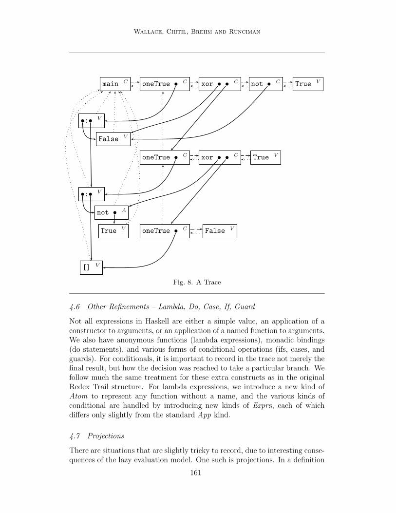
The augmented version of the Redex Trail graph from Figure 2 is shown inFigure 8. The subexpression relationship is now shown as a pointer (solid line).Parents are shown as dotted lines, and results as dashed lines. Expressionsare annotated with their status .

4.5 Entry Points to the Trace

Every ART viewing tool needs an entry point at which to begin its presentationto the user. These entry points can be different for different tools.

The entry point for algorithmic debugging is the ‘beginning’ of the com-putation, the evaluation of the main function. In every ART trace, the Expr

for main is the first Expr in the generated sequence.

The entry point for some other viewers is at the ‘end’ of computation, forinstance when reconstructing a virtual stack-trace from an error message, orwhen exploring a Redex Trail backwards from the program output. This sug-gests that both the program output and any error messages must be recordedin the trace, since they are the ‘end-points’ of the program. Output and errorsare easily added to the ART structure as strings with parent pointers. Theoutput need not be monolithic; it can be spread across many strings; howeverwe do not discuss here the various possible ways to split the output, nor howto store it in the file in a manner that permits quick access.

Other viewers may have variable entry points. For instance, a HOOD-styleobservation may need a named function or source position, and retrieve therelevant information by linear search through the trace.

5 The original Redex Trail structure had a kind of node (Sat) which incorporated aspectsof both the result pointer and the status marker, but these nodes were transient, removedfrom the graph once an expression was evaluated. The Sat node did not permanently recordthe full information required to forward-link every redex to its reduct.

160


True V

not • A

False V

[] V

•:• V

•:• V

False VoneTrue • C

True Vxor • • ConeTrue • C

True Vnot • Cxor • • ConeTrue • Cmain C

Fig. 8. A Trace

4.6 Other Refinements – Lambda, Do, Case, If, Guard

Not all expressions in Haskell are either a simple value, an application of aconstructor to arguments, or an application of a named function to arguments.We also have anonymous functions (lambda expressions), monadic bindings(do statements), and various forms of conditional operations (ifs, cases, andguards). For conditionals, it is important to record in the trace not merely thefinal result, but how the decision was reached to take a particular branch. Wefollow much the same treatment for these extra constructs as in the originalRedex Trail structure. For lambda expressions, we introduce a new kind ofAtom to represent any function without a name, and the various kinds ofconditional are handled by introducing new kinds of Exprs, each of whichdiffers only slightly from the standard App kind.

4.7 Projections

There are situations that are slightly tricky to record, due to interesting conse-quences of the lazy evaluation model. One such is projections. In a definition

161


like id x = x , the question is, who is the parent of x? In one sense, it is id ,yet in another sense, id is merely passing on the value without touching it,so x ’s parent is really whatever expression created it, not id . Once again, wefollow the original Redex Trail structure by introducing another special kindof Expr , the Proj node, which can be thought of as attaching an additionalprojective parent to the referenced redex.

4.8 Trusting

Finally, it is sometimes desirable not to record all reductions in the tracestructure – we trust some function definitions, such as those in the StandardPrelude [10]. There are two main reasons for trusting. The first reason is toimprove performance. Trace files are very large and quite slow to write. If weknow that certain parts of the trace are not of interest, it makes sense to omitthem. The second reason is to reduce the amount of information presented tothe user of a trace-viewing tool. 6 Traces contain a huge amount of data, soa trace that appears too complex can actually hide the information the userwants. We do not elaborate the details of the trusting mechanism here.

5 Multiple Views from a Single Trace

Having outlined a unifying trace structure, we must now demonstrate that itcan satisfy the needs of the Redex Trail, EDT, and Observation views. Wehave built three separate viewers which mimic the user interface behaviour ofthe three previous systems (Freja, HOOD, and the old Hat). In this section,we describe how the required information is reconstructed from the new ARTtrace.

5.1 A Redex Trail View: hat-trail

The original Redex Trail structure can be recovered by following mainly parentpointers. The result pointer chain is used to show a subexpression in its mostevaluated form. The original Hat browser has been adapted to use the newART trace, and is now called hat-trail. The viewer starts with programoutput or an error message, and enables the user to interactively explore acomputation backwards from effect to cause by revealing the parent (origin)of any selected subexpression.

5.2 A Static Call Stack: hat-stack

One special-case use of the parent pointers is to show a static call-stack back-trace from any error message. This does not represent the real lazy evaluationstack — often sadly incomprehensible. Instead the backtrace gives the virtual

6 It would of course be possible to implement a trusting mechanism in the viewing toolitself, rather than omitting the data from the trace altogether.

162


stack showing how an eager evaluation model would have arrived at the sameresult. In our system, this tool is hat-stack.

5.3 Algorithmic Debugging: hat-detect

The tool hat-detect provides Algorithmic Debugging, by extracting a virtualEDT ‘by need’ from the ART trace structure. 7 It can be seen from Figure 4that we need three kinds of information from the trace: first, the EDT’s rootnode; second, an EDT node’s label, where a label is an equation containingan application and its result; and third, the children of an EDT node.

The root node of the EDT is always the main caf, found at the beginningof the trace file.

Each EDT label is an equation: the lhs is an application or caf itself, andthe rhs is its result in its most fully evaluated form. When an App or Const

has a status of Completed , we can follow the result pointer to determine theeventual value. The immediately referenced node might in turn be Completed ,so the result chain must be followed iteratively until we find a node withan Applied , Blackholed or Value status. An Applied node was unevaluated,therefore it cannot have influenced the execution. It is presented to the useras a ‘ ’ symbol. A status of Blackholed is similarly displayed as ⊥. Only aValue status represents a genuine result, either a simple value or a complexstructure, and can be printed as a normal expression.

To determine the children of an EDT node, we must find all fully-evaluatedapplications on which the evaluation of the current node depended. The firstchild of a EDT node p, may be found by following p’s ART result pointer, butthe referenced node q is a child only if its status is Completed or Blackholed .(Only with one of these status annotations does the node describe an appli-cation or caf whose result was actually demanded.) Further children can befound if q is Completed , Blackholed or a Value. In these cases the argumentpointers of q are considered. If an argument’s ART parent is also p, providedthe argument itself is Completed or Blackholed , it is also a child of p. Morechildren can be found recursively by the same method.

In this way, all the information necessary to define a computation’s EDTcan be retrieved from an ART trace file.

Only applications of top-level identifiers are considered by hat-detect. Alocally defined function may depend on the values of free variables bound in anenclosing scope. To decide whether an application appears to be correct, theprogrammer needs to know the values of the free variables, yet the ART tracedoes not record any direct link to these variables. Program errors found byour tool therefore always refer to the top-level function; computation withinlocal definitions is attributed upwards to its enclosing top-level definition.

7 Although we describe the reconstruction of an EDT as if performed in one pass, theimplementation need never build the whole structure - it can be constructed and traversedpiecemeal.

163


The dialogue presented by hat-detect is straightforward to arrange, fol-lowing the standard debugging algorithm. It starts at the root of the EDT,the main caf. If the programmer answers that a node label is erroneous, he isasked about the correctness of its children, but children of nodes identified ascorrect need not be considered. An erroneous node with only correct children,or no children at all, is the location of the bug.

5.4 Observation of Functions: hat-observe

Our tool hat-observe displays all function applications of a given identifierwithin a computation. Unlike HOOD, no annotations are needed in the pro-gram’s source code. As the observed identifier is chosen independently of theprogram run, it is easy to make a number of successive observations withoutmodifying or rerunning the computation.

The tool observes a function by searching sequentially through the tracefile. First, the identifier itself is found as a Const node containing an Id atomwith the name. (See structures in Figures 7 and 3). Then every applicationnode is checked for a reference to the given Const in the function position.

To deal with partial applications we must search the ART trace not onlyfor references to the original Const node, but for references to any applicationwhich in turn references the Const , and so on recursively. If the functioninvolved in an application is a reducible expression (with a function as result)we must follow this expression’s forward result link, to see whether it is thedesired function, or a partial application of it. The cost of such searching fromapplication nodes to determine the associated function turns out to be low,as the relevant expressions are usually found close to the original applicationnode. In particular, an additional file access is very rarely needed, as theseexpressions are usually within the file’s buffer. Linearisation ensures that thefunction reference in an application node can only refer to an earlier node inthe trace 8 , so a single linear scan through the trace is sufficient to collect allapplications of a specified function.

Not all applications or cafs have results – they may be unevaluated, oran application may be partial – but where a result is available, the rhs of theequation can be determined as described in Section 5.3. All applications orcafs with results are displayed as a list of equations.

To avoid redundant output, equivalent or less general applications of theidentifier can be omitted in the display. One application of an identifier isconsidered more general than another if all its arguments are less defined (dueto lazy evaluation). To avoid problems with local functions capturing freevariables, as described in Section 5.3, we again only permit observations oftop-level functions.

Our tool shows all applications of the function throughout the program,whereas HOOD observes a specific function application at one point in the

8 All Ref s in the ART structure, apart from the result , refer to earlier nodes.

164


source code. However, because the source code position is recorded in theART trace, an equivalent feature could be achieved by a different interface,perhaps a source code browser allowing the user to select expressions to beobserved.

6 Trace Generation

The developers of Freja, Hat and HOOD made different choices about thearchitectural level at which they implemented the creation of the trace. Forinstance, in HOOD the trace is created by the combinator observe definedin a high-level Haskell library, which uses side-effecting I/O to record theinformation. In Freja the trace is created in the heap by low-level variants ofthe graph reduction machine instructions [5].

To generate the new ART trace [11] we took the old Redex Trail ap-proach, but adapted to write traces to file instead of constructing them inheap memory. First, the original program is transformed into a new pro-gram that computes its trace in addition to its normal result. Second, thetransformed program is compiled. Third, the compiled program is run. Thecomputation writes a trace to file in addition to any normal I/O of the originalprogram. Fourth, the trace is viewed.

Currently the program transformation is performed by an early phase ofthe Haskell compiler nhc98. However, we intend to separate the transforma-tion from the compiler, so that the transformed program can be compiled withall Haskell compilers. The Augmented Redex Trail approach is then poten-tially as portable as the HOOD implementation, in contrast to Freja. Theprinciple of using an automatic source-to-source transformation, coupled witha library of combinators written in standard Haskell, permits the possibilityof using any Haskell compiler system to generate an ART trace.

6.1 The Program Transformation

The transformation wraps every expression of the original program into theR data type, which is defined as follows:

data R α = R α Ref

The Ref is a reference to an Expr node of the trace in file. The pairingassures that an expression and its description “travel together” throughoutthe computation, so that when expressions are plumbed together by applica-tion, the corresponding descriptions in the trace can be plumbed together bycreating an App node at the same time. Trace nodes are written to file byside-effects which are triggered when certain expressions are evaluated. Allthe plumbing and writing of trace nodes is performed by combinators whichare defined in a library.

165


The program transformation introduces numerous calls of the combina-tors into the program. For example, here is the original oneTrue definition,together with its transformed version.

oneTrue :: [Bool ] → Bool

oneTrue [] = False

oneTrue (x : xs) = xor x (oneTrue xs)

oneTrue :: SrcPos → Ref → R (Ref → (R [Bool ]) → R Bool)oneTrue sr p = fun1 (mkAtomId “oneTrue” 7) oneTrueW sr p

where

oneTrueW :: Ref → R [Bool ] → R Bool

oneTrueW p ′ (R [] ) =

con0 (mkSrcPos 2) p ′ False (mkAtomId “False” 6)oneTrueW p ′ (R (x : xs) ) =

rap2 (mkSrcPos 3) p ′ (xor (mkSrcPos 3) p ′) x

(ap1 (mkSrcPos 4) p ′ (oneTrue (mkSrcPos 4) p ′) xs)

In this example the combinators fun1, con0, ap1, rap2, mkAtomId , andmkSrcPos are used. The combinator fun1 wraps the function oneTrueW ,which does the actual work, with R constructors. The combinator con0 wrapsthe constructor False. The combinators ap1 and rap2 assure the correctplumbing of applications. The combinators mkAtomId and mkSrcPos buildreferences to detailed information about the identifier oneTrue, the construc-tor False and various source references. Numeric arguments are indexes totables that contain the detailed information.

Very similar combinators were used in the old Hat system. The mostimportant difference is that the new Hat combinators now record the tracenodes directly to file.

6.2 Writing with Updating

The main technical obstacle is that the trace is a (usually cyclic) graph whichis continuously modified during generation. These modifications were no prob-lem in main memory but for efficient writing to file updates have to be min-imised.

We assume that writing nodes to file has much better performance if it canbe achieved sequentially. However, even a cursory examination of the ARTstructure tells us that after writing an Expr node to file, it is highly likelythat we will need to return to it to update the result pointer. Although someexpressions remain completely unevaluated throughout the computation, thevast majority of intermediate expressions are indeed entered and evaluated totheir reduct.

166


What is more, in our scheme there are two possible updates for each Expr ,one on entering the expression (Applied → Blackholed), and another on itscompletion (Blackholed → Completed).

However, we observe that a Blackholed expression is almost always tran-sient. The only situation in which such an annotation can remain in the finaltrace is when the program’s overall result is undefined, such as an error orinterruption. We also observe that the order in which trace expressions areentered and then completed follows a strict stack discipline, mirroring theevaluation stack of the underlying abstract machine. Hence, we do not up-date Applied to Blackholed on entry, but only write the remaining stack of‘blackholes’ at the end of the computation should it fail.

We also try to avoid interspersing the final update of each Expr with thesequential generation of nodes. This is easily achieved by storing a large queueof updates that are performed all at once.

7 Future Work

The practical questions that interest most people are about time and space.How large is the trace? And how long does it take to produce, relative to theoriginal computation?

An ART trace is undoubtedly big, to be measured in megabytes for a com-putation of any significant size. We estimate about 40–50 bytes are requiredper reduction. The largest trace we have yet generated is 240Mb in size, for acomputation of around 6 million reductions (a chess end-game solver). Tracedcomputations also take about 50 times longer than normal computations.

If Hat is to be used for substantial computations, we have to reduce theslow-down factor for traced computations. The fact that only 10% of tracedcomputation time is spent on actually writing to file demonstrates that theimplementation of trace generation can be improved. Since the computationof a transformed program spends most of its time evaluating the combinators,efficient definitions of the combinators are vital. We will also separate theprogram transformation from nhc98, so that a transformed program can becompiled by an optimising Haskell compiler such as ghc. Not only would thisimprove absolute runtimes, but aggressive optimisation may also reduce therelative slow-down. Furthermore, the computation of trusted function defini-tions is not yet much faster than that of untrusted definitions. We intend toinvestigate how transformed modules can be combined with trusted untrans-

formed modules. Such a scheme, not requiring access to the sources of trustedmodules, would also aid portability.

Other issues we want to address include:

• Currently I/O actions are traced in a rather ad hoc way that works wellonly with some views for simple I/O only. We aim to develop a generalmethod for tracing I/O actions.

167


• We want to solve the problem that none of the views copes well with pro-grams that make substantial use of higher-order combinators, for examplein monadic or continuation-passing style.

• We plan to extend hat-observe to observe values at any program point.We could also add information about free variables to expressions in thetrace, so that hat-detect and hat-observe can show a fuller trace of localcomputation. It may even be desirable to switch levels of detail within aview.

• There is scope for new viewing tools. For instance, the evaluation order ofthe computation is stored implicitly in the sequence in which Expr nodesare written to file. Hence, the computation, or selected parts of it, could beshown as an “animation”, perhaps in the style of GHood 9 . We could alsooffer a “stories” view in the style outlined in [1]. A more specialised toolcould isolate the circular self-dependency that evokes a “blackhole” error.

• We have begun to integrate hat-detect and hat-observe into a singletool. Eventually we hope for a full integration allowing the programmer toswitch between views at any point during the exploration of a computation.

• How can we evaluate the useability of Hat in practice and gain informationto improve it?

More generally, we intend to study the properties of the ART trace fur-ther. Is the trace complete with respect to information, such as recorded re-ductions, intermediate unevaluated expressions and values, and with respectto distinctions and relationships, such as sharing and evaluation order? Howconveniently and efficiently can one access the trace to obtain a specific snip-pet of information? Can we claim some sort of “universality” for the tracestructure, in terms of the range of queries it can support? How are all theseproperties affected by trusting? Does the exclusion of trusted redexes from thetrace compromise the reachability of individual trace nodes from designatedentry points?

There should be a close relationship between tracing and operational se-mantics, both of which aim to describe the relationship between a program andthe observed actions of a computation of the program. We have begun work todefine the ART trace and specific views through conservative extensions of anoperational semantics of a program. Different kinds of formal semantics maysuggest new views for tracing. For instance, the evaluation dependency tree ofalgorithmic debugging is closely related to a big-step structured operationalsemantics; the Redex Trail view was inspired by graph-rewriting machines;the observation of values recalls denotational semantics, especially the view offunctional values as (finite) mappings (‘minimal function graphs’ [4]).

In principle, a semantics defines all the answers a tracer could give forthe computation of a particular program with particular input. A tracer

9 http://www.cs.ukc.ac.uk/people/staff/cr3/toolbox/haskell/GHood/

168


makes this information available. A tracer avoids providing its own semanticsbut hooks on to a compiler instead. A program transformation provides this“hook” in a portable way. Even more important than the information in atrace is its accessibility.

8 Conclusions

We have presented the new modular architecture of our Haskell tracer Hat.At its heart lies the new Augmented Redex Trail trace structure, designed onthe one hand to be written to file while performing the traced computation,and on the other hand to provide data sufficient for multiple views.

As an immediate result, we have widened the applicability of the new Hatconsiderably. Initial experiences confirm the usefulness of generating a traceonly once and viewing it in several different ways.

The new modularity improves the understanding of the tracing process.The new architecture has also prompted us to ask some more general questions,such as those in the Future Work section.

9 Acknowledgements

Many thanks to Amanda Clare, Henrik Nilsson, John O’Donnell, Claus Reinke,and Jan Sparud who each took time to travel to York and play with variousdifferent tracing systems. The feedback from these experiments was extremelyvaluable.

We also thank the referees for their constructive comments.

The work reported in this paper was supported by the UK’s Engineeringand Physical Sciences Research Council under grant number GR/M81953.

References

[1] Simon P Booth and Simon B Jones. Walk backwards to happiness — debuggingby time travel. Technical Report CSM-143, University of Stirling, 1997.

[2] Olaf Chitil, Colin Runciman, and Malcolm Wallace. Freja, Hat and Hood— A comparative evaluation of three systems for tracing and debugginglazy functional programs. In Markus Mohnen and Pieter Koopman, editors,Implementation of Functional Languages, 12th International Workshop, IFL2000, LNCS 2011, pages 176–193. Springer, 2001.

[3] Andy Gill. Debugging Haskell by observing intermediate data structures. In2000 ACM SIGPLAN Haskell Workshop, 2000. Technical Report NOTTCS-TR-00-1, University of Nottingham.

[4] N. D. Jones and A. Mycroft. Data Flow Analysis of Applicative Programs usingMinimal Function Graphs. In Proc. 13th Annual Symposium on the Principles ofProgramming Languages (POPL’86), pages 296–306, ACM Press, January 1986.

169


[5] Henrik Nilsson. Declarative Debugging for Lazy Functional Languages. PhDthesis, Linkoping, Sweden, May 1998.

[6] Henrik Nilsson and Jan Sparud. The evaluation dependence tree as a basis forlazy functional debugging. Automated Software Engineering: An InternationalJournal, 4(2):121–150, April 1997.

[7] Claus Reinke. GHood — Graphical visualisation and animation of Haskell objectobservations. Proceedings of ACM Sigplan Haskell Workshop 2001, September2001.

[8] E. Y. Shapiro. Algorithmic Program Debugging. MIT Press, 1983.

[9] Jan Sparud. Tracing and Debugging Lazy Functional Computations. PhD thesis,Chalmers University of Technology, Goteborg, Sweden, 1999.

[10] Jan Sparud and Colin Runciman. Complete and partial redex trails offunctional computations. In C. Clack, K. Hammond, and T. Davie, editors,Selected papers from 9th Intl. Workshop on the Implementation of FunctionalLanguages (IFL’97), pages 160–177. Springer LNCS Vol. 1467, September 1997.

[11] Jan Sparud and Colin Runciman. Tracing lazy functional computations usingredex trails. In H. Glaser, P. Hartel, and H. Kuchen, editors, Proc. 9th Intl.Symposium on Programming Languages, Implementations, Logics and Programs(PLILP’97), pages 291–308. Springer LNCS Vol. 1292, September 1997.

170

multiple-view tracing for haskell: a new hat

Documents