Multiples and Their Valuation Accuracy

in European Equity Markets*

Andreas Schreiner and Klaus Spremann**

August 13, 2007

* We would like to thank David Aboody, Thomas Berndt, Jan Bernhard, Pascal Gantenbein, Sebastian

Lang, Jing Liu, Jacob Thomas, and seminar participants at UCLA, University of Innsbruck, University of

St.Gallen, and Yale University for helpful comments. Financial support for this study by the Swiss Na-

tional Science Foundation and provision of data by Thomson Financial is gratefully acknowledged.

** Andreas Schreiner: Visiting Assistant in Research / Postdoctoral Fellow, Yale University, School of

Management; Research Associate, Swiss Institute of Banking and Finance, University of St.Gallen; Klaus

Spremann (communicating author): Professor and Director, Swiss Institute of Banking and Finance, Uni-

versity of St.Gallen; Mail: klaus.spremann@unisg.ch; Tel.: +41-71-224-7074.

2

Abstract

In spite of their widespread use in practice, accounting-based market multiples are sub-

ject of surprisingly few academic studies. As a contribution to close this gap, we exam-

ine the accuracy of different types of multiples in European equity markets. We find

that multiples generally approximate market values reasonably well. In terms of relative

accuracy, our results show: (1) Equity value multiples outperform entity value multi-

ples. (2) Knowledge-related multiples are more accurate than traditional multiples. (3)

Forward-looking multiples, in particular the two-year forward-looking price to earnings

(P/E) multiple, outperform trailing multiples. These empirical findings are significant in

magnitude, robust to the use of different performance measures, and constant over time.

In an out-of-sample test using a U.S. dataset, our results for European data are con-

firmed. This supports the relevance of our findings for practical purposes.

JEL-Classification: G15, G24, M41.

Keywords: Finance and Accounting, Equity Valuation, Multiples.

3

1 Introduction

Accounting-based market multiples are most commonly applied to corporate valuation.

These multiples are ubiquitous in analysts’ reports and investment bankers’ fairness

opinions. They also appear in valuations associated with transactions of corporate con-

trol. The Multiples Valuation Method (MVM) is very intuitive. Unlike the Dividend

Discount Model (DDM), the Discounted Cash Flow (DCF) approach, or the Residual

Income Model (RIM) Model, the MVM does not require detailed multi-year forecasts of

dividends, free cash flows or residual incomes. Instead, the firm being valued gets asso-

ciated with a peer group of firms considered to be comparable. A simple analysis of the

stock prices of the firms in the peer group leads to a certain ratio which will then be

used as a multiplier of the target firm’s value driver. Despite the widespread use of the

MVM, only limited theory is available to support the application. Studies on the empiri-

cal accuracy are scarce, and with a few exceptions, the literature gives no support on

why certain multiples should be chosen in specific contexts.

This paper investigates the empirical accuracy of the MVM using a broad European

dataset. We explore the properties of various types of multiples and aim to give recom-

mendations regarding three choices which must be made for the MVM: (1) Should a

multiple concentrate on the equity value or on the entity value of the firm? (2) Should a

multiple relate on knowledge-related value drivers or on traditional ones? (3) Should

forward-looking multiples be preferred to trailing multiples? An innovation in our

analysis is the focus on European data. Nevertheless, we also consider U.S. data to vali-

date our results and to make them comparable to existing studies (which are typically

based on U.S. data).

2 Literature overview

Multiples are subject of surprisingly few academic studies. Among the first studies, Al-

ford (1992) uses P/E multiples to test the effects of different methods of identifying

comparable firms based on industry membership and proxies for growth and risk on the

accuracy of valuation estimates: The outcome of the MVM is compared to observed

market prices of common stock. He finds that valuation accuracy increases when the

fineness of the industry definition used to identify comparable firms is narrowed from

4

1-digit to 2-digit and 3-digit industry codes, but there are no further improvements when

4-digit industry codes are considered. He also finds that adding controls for earnings

growth, leverage, and size does not significantly reduce valuation errors.

Kaplan & Ruback (1995) investigate properties of the DCF model in the context of

private equity transactions. While they conclude that DCF valuations approximate

transaction values reasonably well, they also find that simple enterprise value to earn-

ings before interest, taxes, depreciation, and amortization (EV/EBITDA) multiples re-

sult in similar valuation accuracy. Gilson, Hotchkiss & Ruback (2000) compare the

market value of firms that recognize bankruptcy to value estimates from the DCF model

and the MVM. As in Kaplan & Ruback (1995), the DCF and the multiples approach

have about the same degree of valuation accuracy.

In a more general context, Liu, Nissim & Thomas (2002) investigate the perform-

ance of multiples for the U.S. equity market. They find that multiples based on earnings

forecasts explain stock prices well for a large fraction of firms. That is, inverse P/E mul-

tiples using two-year earnings per share (EPS) forecasts generate valuations within

twenty percent of observed prices for almost sixty percent of firm years. The authors

also compare their results with the performance of the RIM. Against their intuition, the

RIM performs worse than the multiples approach. In a recent study, Liu, Nissim &

Thomas (2007) extend their analysis and examine the performance of earnings versus

cash flow multiples in a more international setting. Across ten countries, they find that

multiples based on earnings measures outperform those based on operating cash flow

and dividends. Moving from trailing numbers to forecasts improves the valuation accu-

racy, with the greater improvement being observed for earnings.

Consistent with the results of Liu, Nissim & Thomas (2002 and 2007), Kim & Rit-

ter (1999) conclude how IPO prices are set using multiples. They show that forward-

looking P/E multiples outperform all other multiples in accuracy. In fact, two-year EPS

forecasts dominate one-year EPS forecasts, which in turn dominate current EPS. Lie &

Lie (2002) examine the accuracy of a conventional list of multiples for the universe of

firms within the Compustat North America database. In line with the preceding studies,

they also report superior performance of forward-looking P/E multiples compared to all

other multiples.

5

3 Methodology

3.1 Definition and categorization of multiples

Following Penman (2004), we define a (market) multiple as the ratio of a market price

variable (such as the stock price, the market capitalization, or the whole enterprise

value) to a particular value driver (such as earnings, revenues, or the work force) of a

firm. This definition enlightens that the MVM finds prices (in a particular market set-

ting, reflecting the current market sentiment) rather than values (which are defined as

prices in a perfect market and therefore estimated on the basis of “long-term data” and

“typical conditions”).

A multiple is called to be consistent, if there is an accepted economic model which

explains (under certain assumptions) a proportional relationship between the value

driver and value. For example, Gordon’s growth model comes up with the notion that

the value of equity ,

equity

i tv of firm i at time t equals the expected next dividend dt+1 di-

vided by the difference between the discount rate r and the growth rate g. Thus, value is

equal to the product of the expected next dividend (value driver) and the constructed

multiple 1/( )= −m r g

[ ]

[ ]1

, 1

+

+= = ⋅−

tequity

i t t

E dv m E d

r g (1)

Here, the multiple depends only on the risk of the firm (which is reflected in the

cost of capital) and the growth rate. The underlying belief of the MVM is that multiples

are the same within a group of comparable firms and within a certain time window.

Thus, the size of the multiple must not be inferred from a model like Gordon’s. It can be

empirically determined by observing the actual market prices and value drivers for a

few firms which are, by a precedent analysis, identified as comparable. The resulting

synthetic multiple is then used to estimate the value of the target firm for which only the

value driver is known. If the actual price of the target firm can be observed, the differ-

ence between the actual price and the value estimated using the MVM serves to assess

the accuracy of the method. The accuracy determines the performance of the MVM.

6

Our analysis attempts to find multiples which are both consistent and accurate (high

performance).

The MVM requires four steps. Step 1 is the selection of the kind of value under in-

terest (such as equity or entity) and of the value driver (such as earnings or cash flows).

Step 2 identifies the group of comparable firms, the peer group. Together with the mar-

ket price variables, the value drivers form the basis for the calculation of the corre-

sponding multiples of the comparables. Step 3 aggregates these individual multiples

into a single number. This procedure is carried out by estimating synthetic peer group

multiples according to a chosen statistical measure of central tendency. Step 4 deter-

mines the value estimation for the target firm by taking the product of the synthetic peer

group multiple and the value driver of the firm being valued.

The general definition of a multiple allows for a variety of different multiples. In

order to analyze specific characteristics of multiples, we use a two dimensional catego-

rization scheme as shown in Figure 1. The first dimension refers to the numerator of the

ratio and differentiates between equity value and entity value multiples. Equity value

multiples are based on the stock price or the market capitalization of a firm, whereas

entity value multiples are based on the enterprise value of a firm. Formally, an equity

value multiple ,

equity

i tλ of firm i at time t is

,

,

,

equity

i tequity

i t

i t

p

xλ = (2)

where ,

equity

i tp is the current market value of common equity and ,i tx is the underly-

ing value driver of the multiple. Similarly, an entity value multiple ,

entity

i tλ of the same

firm at time t can be written as

, , ,

,

, ,

ˆentity equity net debt

i t i t i tentity

i t

i t i t

p p p

x xλ

+= = (3)

where ,

entity

i tp is the current enterprise value which equals the sum of the market

value of common equity ,

equity

i tp and an estimator of the market value of net debt

,ˆ net debt

i tp ,

7

and ,i tx is again the value driver.1 The origin of the value driver ,i tx in the financial

statement constitutes the main differentiation criteria for the second dimension of the

categorization framework, where we distinguish (1) accrual flow, (2) book value, (3)

cash flow, (4) knowledge-related, and (5) forward-looking multiples. The first three

types of multiples are referred to as traditional or trailing multiples.

3.2 Hypotheses

Equity value versus entity value multiples

One of the first questions is how the chosen market price variable – market capitali-

zation (equity value) or enterprise value (market capitalization plus book value of net

debt) – determines the accuracy of the MVM. When working with entity value multi-

ples, one should preserve consistency by “matching” the economic meaning of the nu-

merator with that of the denominator. Entity value multiples should utilize value drivers

in the denominator which are defined on an enterprise level. Equity value multiples

should be constructed from value drivers that are defined on an equity holder’s level.

Otherwise, the multiple may be incomparable with economic reasoning, although it

could lead to acceptable results in practice. The principle of consistency is often vio-

lated, however. P/SA, P/EBIT(DA), or P/OCF multiples are widely used for equity

valuations.2 The level of debt, or more precisely the capital structure, can create prob-

lems that impact the consistency of equity value multiples.

In a Modigliani & Miller (1958) world without taxes, costs of financial distress, and

other agency costs, different capital structures across firms affect equity value multiples,

if they are not defined on an equity holder’s level. In such a world, managers can con-

trol specific equity value multiples by swapping debt for equity and thereby varnish the

attractiveness of their firm to investors. In a real world setting, taxes, costs of financial

distress, and agency costs exist, shaping tradeoffs between debt and equity and making

1 Net debt is defined as total debt less cash & equivalents plus preferred stock. Since the market value of

net debt net debt

p is usually not publicly available, we approximate net debt

p with the book value of net debt

net debtb and write

ˆ

net debtp to indicate the approximation.

2 In our empirical study, we ignore the matching principle for equity value multiples to directly compare

the empirical performance of equity value versus entity value multiples.

8

capital structure value relevant. The tax benefits of higher leverage are opposed by an

increasing probability of default and costs of financial distress. As a compensation for

the increase in risk and the decrease in flexibility, shareholders demand higher returns

and the value decreases (see Myers (1977)). The consideration of agency costs favors

the use of debt over equity (see Ross (1977) or Myers (1984)). If capital structure mat-

ters, financing decisions influence the value of a firm and thus both equity value and

entity value multiples. Entity value multiples are less affected because they are defined

on an enterprise level. Consistent entity value multiples are difficult to establish, how-

ever. The reason is that we cannot observe the enterprise value of a firm since the true

value of debt is not established through market prices. In the MVM the value of net debt

is therefore measured by its book value. This approximation can produce uncontrollable

uncertainty, especially in a changing interest rate and default risk market environment.

Moreover, the composition and calculation of net debt in the balance sheet can vary sig-

nificantly across firms, producing even more noise. Needless to say that firms belonging

to the same peer group can have different kinds of debt and levels of cash & equiva-

lents. There may also be differences in the treatment of pension liabilities, employee

stock options, or capitalized leases. Some firms have preferred stock or off-balance

sheet items such as operating leases and special purpose entities.

Taken together, when comparing the features of equity value versus entity value

multiples, the latter appeal in the view of consistency because they are less affected by

capital structure. Equity value multiples can compensate for this theoretical drawback in

practice because the market capitalization in the numerator can be directly observed

from market prices and therefore does not suffer from uncontrollable uncertainty. The

fact that firms from the same industry tend to operate at similar debt levels, gives equity

value multiples another advantage. This leads to Hypothesis 1: Equity value multiples

outperform entity value multiples in valuation accuracy.

Knowledge-related versus traditional multiples

For the proposition of Hypothesis 2 and Hypothesis 3, we shift the attention to the

denominator of a multiple as a ratio and specific value drivers in different industries.

Throughout the last two decades, the corporate landscape has changed with the

achievements and developments in information and internet technology. Nowadays, in-

vesting in research and development (R&D) is a major indicator of productivity, par-

9

ticularly for firms in science-based industries. From an accounting perspective, R&D

differs from other capital inputs such as physical property, plant and equipment, inven-

tory, or project financing. While most accounting standards mandate the capitalization

and periodic depreciation of physical forms of long-term investment, R&D is in most

cases immediately expensed in financial statements. This produces earnings figures

which underestimate “true” earnings (e.g., Lev & Sougiannis (1996), Aboody & Lev

(1998 and 2000), or Eberhart, Maxwell & Siddique (2004)). Consequently, adding back

R&D expenditures to EBIT or net income yields earnings figures of “higher quality” in

the perspective of corporate valuation.

If accounting standards change and firms capitalize R&D, it would appear as an in-

tangible asset on the balance sheet. Examples of such assets without physical substance

are brand names, copyrights, goodwill, leasehold rights, licenses, patents, or software.

Some amortization may be appropriate for intangibles. Hitherto, all international ac-

counting standards (but U.S.-GAAP) mandate the amortization of capitalized intangible

assets (AIA) over their expected “useful” lives. For many intangible assets, however,

law or regulation prescribe the useful amortization time based on conservative account-

ing. Again, reported amortization expenditures exaggerate the “true” decrease in the

value of intangible assets. Both the immediate expense of R&D and the principle of sys-

tematic AIA diminish the quality of reported earnings and consequently the quality of

multiples based on earnings. To correct these consequences of accounting conservatism

and to produce a more reliable picture of a firm’s true economic success or value, we

suggest adding back R&D expenditures and/or amortization to EBIT and net income in

science-based industries (i.e., all industries with a substantial exposure to intangible as-

sets or R&D, or both of them).3 The “and/or” decision depends on the magnitude and

consistency of R&D expenditures and amortization within an industry. That is, if R&D

expenditures (amortization costs) are relatively low or come with high volatility, we are

better off adding back only amortization (R&D expenditures). On the other hand, if both

numbers are of considerable size and stable, we should sum them up into a single num-

ber. We define the sum of R&D expenditures and amortization of intangible assets as

3 Based on the Industry Classification Benchmark (ICB) system, our definition of science-based indus-

tries contains Oil & Gas, Basic Materials, Industrials, Health Care, Telecommunications, Utilities, and

Technology.

10

costs for the creation and maintenance of intangible assets or short knowledge costs

(KC). According to this, we argue that knowledge-related multiples outperform tradi-

tional multiples in science-based industries (Hypothesis 2).

Forward-looking versus trailing multiples

In the MVM, the value driver in the denominator of the ratio is often chosen to be

one of the latest numbers in the financial statements for the recent fiscal quarter or year.

These multiples are called trailing, because the numbers are based on historical data. If

the value driver of a multiple refers to a forecast instead of a historical number, it is

termed forward-looking. Since the value of a firm equals its discounted stream of ex-

pected future payoffs, forward-looking multiples may have an advantage with respect to

consistency. Empirical research for the U.S. underpins that forward-looking multiples

are more accurate than trailing multiples. In a sample of 142 U.S. IPOs, Kim & Ritter

(1999) find that P/E multiples based on earnings forecasts for the subsequent two years

outperform those based on historical earnings. As their analysis moves from trailing to

one-year and to two-year ahead forward-looking multiples, the percentage of firms val-

ued within 15 percent of their actual stock price increases from 15 percent to 19 percent

and then to 36 percent. Liu, Nissim & Thomas (2002) show similar results in their broad

investigation of U.S. equity markets. The median valuation error equals 23 percent for

inverse P/E multiples based on historical earnings and falls to 18 percent and 16 percent

when moving to one-year and two-year forward-looking multiples. The two studies are

appealing because earnings forecasts should reflect future profitability and growth better

than historical measures. The accuracy increases by lengthening the forecast horizon

from one year to two years.

Based on the principles of valuation and on empirical evidence, we recommend

forward-looking multiples whenever forecast data for the multiples is available for the

entire peer group. Since analysts’ practice is to make point in time estimates of earnings

measures for only two years ahead, the most promising choice are forward-looking mul-

tiples processing two-year ahead forecasts. Forecasts on a broad basis are typically

available for EBIT(DA), pre-tax income, and net income. Hypothesis 3 states that for-

ward-looking multiples outperform trailing multiples.

11

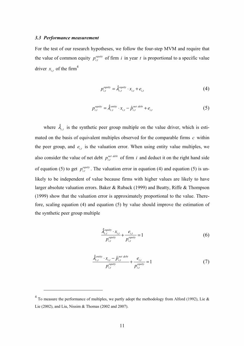
3.3 Performance measurement

For the test of our research hypotheses, we follow the four-step MVM and require that

the value of common equity ,

equity

i tp of firm i in year t is proportional to a specific value

driver ,i tx of the firm4

, , , ,ˆequity equity

i t c t i t i tp x eλ= ⋅ + (4)

, , , , ,ˆ ˆequity entity net debt

i t c t i t i t i tp x p eλ= ⋅ − + (5)

where ,ˆc tλ is the synthetic peer group multiple on the value driver, which is esti-

mated on the basis of equivalent multiples observed for the comparable firms c within

the peer group, and ,i te is the valuation error. When using entity value multiples, we

also consider the value of net debt

,

net debt

i tp of firm i and deduct it on the right hand side

of equation (5) to get ,

equity

i tp . The valuation error in equation (4) and equation (5) is un-

likely to be independent of value because firms with higher values are likely to have

larger absolute valuation errors. Baker & Ruback (1999) and Beatty, Riffe & Thompson

(1999) show that the valuation error is approximately proportional to the value. There-

fore, scaling equation (4) and equation (5) by value should improve the estimation of

the synthetic peer group multiple

, , ,

, ,

ˆ1

equity

c t i t i t

equity equity

i t i t

x e

p p

λ ⋅+ = (6)

, , , ,

, ,

ˆ ˆ1

entity net debt

c t i t i t i t

equity equity

i t i t

x p e

p p

λ ⋅ −+ = (7)

4 To measure the performance of multiples, we partly adopt the methodology from Alford (1992), Lie &

Lie (2002), and Liu, Nissim & Thomas (2002 and 2007).

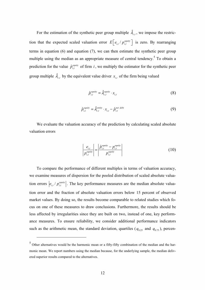
12

For the estimation of the synthetic peer group multiple ,ˆc tλ , we impose the restric-

tion that the expected scaled valuation error , ,/ equity

i t i tE e p is zero. By rearranging

terms in equation (6) and equation (7), we can then estimate the synthetic peer group

multiple using the median as an appropriate measure of central tendency.5 To obtain a

prediction for the value ,ˆ equity

i tp of firm i , we multiply the estimator for the synthetic peer

group multiple ,ˆc tλ by the equivalent value driver ,i tx of the firm being valued

, , ,ˆˆ equity equity

i t c t i tp xλ= ⋅ (8)

, , , ,ˆˆ ˆequity entity net debt

i t c t i t i tp x pλ= ⋅ − (9)

We evaluate the valuation accuracy of the prediction by calculating scaled absolute

valuation errors

, , ,

, ,

ˆ equity equity

i t i t i t

equity equity

i t i t

e p p

p p

−= (10)

To compare the performance of different multiples in terms of valuation accuracy,

we examine measures of dispersion for the pooled distribution of scaled absolute valua-

tion errors , ,/ equity

i t i te p . The key performance measures are the median absolute valua-

tion error and the fraction of absolute valuation errors below 15 percent of observed

market values. By doing so, the results become comparable to related studies which fo-

cus on one of these measures to draw conclusions. Furthermore, the results should be

less affected by irregularities since they are built on two, instead of one, key perform-

ance measures. To ensure reliability, we consider additional performance indicators

such as the arithmetic mean, the standard deviation, quartiles ( 0.25q and 0.75q ), percen-

5 Other alternatives would be the harmonic mean or a fifty-fifty combination of the median and the har-

monic mean. We report numbers using the median because, for the underlying sample, the median deliv-

ered superior results compared to the alternatives.

13

tiles ( 0.10q and 0.90q ), and the fraction of absolute valuation errors smaller than 25 per-

cent. Characteristics of high accuracy are on one hand small numbers for measures of

central tendency (i.e., median, mean, quartiles, and percentiles) and the standard devia-

tion, and on the other hand high numbers for the fractions of absolute valuation errors

below 15 percent and 25 percent respectively. Any performance indicator is first calcu-

lated for each year. Then, the yearly numbers are aggregated using the average.

4 Data and sample

The indices used in the empirical part of our study are the Dow Jones STOXX 600 and

the S&P 500 index. They represent approximately 85 percent of the total market capi-

talization in Western Europe and 75 percent in the U.S. Hence, they are reliable proxies

for the total markets. Our study concentrates mainly on the European dataset. The

analysis of the U.S. dataset is used to validate the results of the European data by mak-

ing an out-of-sample test. The Dow Jones STOXX 600 index contains the 600 largest

stocks traded on the major exchanges of 17 Western European countries.6 To classify

firms into different industries and subindustries, we use the ICB system provided by

Dow Jones and FTSE. This industry classification system consists of four levels (in in-

creasing fineness): Ten industries, 18 supersectors, 39 sectors, and 104 subsectors, and

offers four-digit industry codes for all firms within the dataset.

To construct the sample, we merge data from three sources: (1) Historical account-

ing numbers from Worldscope, (2) market prices from Datastream, and (3) analyst fore-

casts from the I/B/E/S. For the ten recent years from 1996 to 2005, we calculate up to

fifty different multiples for each firm i in year t using accounting numbers and mean

consensus analyst forecasts as of the beginning of January and market prices as of the

beginning of April. We measure market prices four months after the fiscal year end to

ensure that all year-end information is publicly available by then and is reflected in

prices.

6 The index universe is constructed by aggregating stocks traded on the major exchanges in Austria, Bel-

gium, Denmark, Finland, France, Germany, Greece, Ireland, Italy, Luxembourg, the Netherlands, Nor-

way, Portugal, Spain, Sweden, Switzerland, and the U.K.

14

The sample considers data that satisfies four criteria: (1) for individual firms, there

are no more than two types of stock (e.g., common stock and preferred stock) traded at

the domestic exchange and an unambiguous dataset is available from the aforemen-

tioned sources; (2) for individual firm years, the market capitalization is above 200 mil-

lion U.S. Dollar ($) and the value of net debt is positive; (3) for individual multiples, the

underlying value driver in the denominator of a multiple is positive, so that negative or

infinite values are impossible; and (4) for the construction of the peer group and eventu-

ally for predicting equity values using multiples, we require the availability of at least

seven comparables within the same industry definition. By doing so, statistical outliers

cannot distort the empirical results. In addition, the analysis is conducted out-of-sample,

which means that the target firm is not part of the peer group.

The resulting sample for the Dow Jones STOXX 600, which consists of 592 firms,

is used for the descriptive statistics reported in panel B of Table 1. The median firm has

annual sales of $3.56 billion, annual net income of $206 million, total assets of $5.83

billion, book value of common equity of $1.68 billion, and pays an annual dividend of

$85 million. Thus, the median net profit margin and the median return on common eq-

uity equal 5.79 percent and 12.28 percent respectively. Firms also operate with consid-

erable leverage at a debt to equity ratio of about two to one. However, note that all of

the financial characteristics are heavily skewed to the right, as indicated by the large

differences between the medians and the means. For most numbers the mean is even

higher than the number for the third quartile.

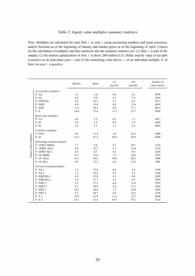
Table 2 presents summary statistics of the investigated equity value multiples. The

median values of common equity value multiples are 16.8 for the P/E multiple, 2.1 for

the P/B multiple, and 1.1 for the P/SA multiple. Reflecting analysts’ overall expecta-

tions of positive future growth, in particular earnings growth, one-year forward-looking

multiples are higher than the corresponding trailing multiples but lower than the corre-

sponding two-year forward-looking multiples. Interestingly, the median P/TA multiple

is 0.6, whereas the median P/IC multiple is 1.0, which indicates that firms in Europe

operate with a considerable high balance of cash & equivalents. This observation is es-

pecially evident for the second half of the time horizon of the study. Also, note that the

number of observations is smaller for knowledge-related multiples and forward-looking

multiples compared to traditional multiples. The former are restricted to science-based

15

industries. Moreover, several national accounting regimes do not require firms to sepa-

rately disclose their R&D and amortization expenditures in their income statement. The

availability of forward-looking multiples is limited because the I/B/E/S database pro-

vides analyst forecasts only for the last six years of the study. Again, the distribution of

multiples is positively skewed.

5 Results

5.1 Absolute valuation accuracy

Indicators of valuation accuracy for equity value multiples within the European sample

are reported in Table 3. This table presents the absolute valuation accuracy and under-

lines, that the MVM can explain equity market values correctly: For 18 out of 27 differ-

ent equity value multiples, the median absolute valuation error lies below thirty percent

(first column). Half of the value predictions deliver results no more than thirty percent

above or below the actual market value of common equity. Five multiples yield median

absolute errors of less than 25 percent. The median errors range from 21.5 percent to

43.8 percent.

Presented in the second column from the right of Table 3, the fraction of absolute

valuation errors within 15 percent of observed market values varies from 22.4 percent to

40.0 percent. As a comparison, Lie & Lie (2002) report a variation between 22.5 percent

and 35.1 percent using ten different multiples for U.S. equity data. The percentage of

errors smaller than 15 percent lies above thirty percent for 19 multiples. That is, thirty

percent or more valuations deliver results no more than 15 percent above or below the

market capitalization of the target firm.

The accentuated fields in Table 3 indicate the best performing multiples in each

category. Multiples based on value drivers closer to the bottom line of the income

statement perform better than multiples based on value drivers further up in the income

statement. This observation is not restricted to accrual flow multiples, but also applies to

knowledge-related and to forward-looking multiples. The weak performance of the P/E

multiple compared to the P/EBT multiple does not surprise because corporate tax rates

vary within European countries. Thus, the comparability of net income across firms

from different countries is limited. Comparing book values and earnings as the two most

16

popular accounting value drivers, our study finds that multiples based on earnings

clearly outperform those based on book values. Throughout the cross-section, book

value multiples as well as cash flow multiples disappoint in their ability to explain mar-

ket values. The poor performance of cash flow multiples contradicts the belief that cash

flow measures are better than accrual flow measures in representing future payoffs.

Analyzing the numbers for the additional performance indicators shown in the re-

maining four columns of Table 3 corroborates the findings using the key performance

measures. All this supports the high accuracy of the MVM.

5.2 Equity value versus entity value multiples

The requirement of consistency favors entity over equity value multiples because they

are less affected by different capital structures among comparable firms. In practice the

estimation procedure of the market value of net debt involves considerable uncertainty.

There is a tradeoff between the desired independence of the capital structure and noise

when selecting appropriate multiples. Most prior studies cover only one of the two types

of multiples and thus do not assess differences in the quality of value predictions. Stud-

ies, which consider both types (i.e., Alford (1992) and Liu, Nissim & Thomas (2002))

find evidence for the superiority of equity value multiples, but are unable to provide any

rationale why such results might be observed.

Table 4 presents the results of the evaluation of equity value versus entity value

multiples. To isolate the performance impact of the multiples selection to the market

price variable used, we reduce the universe of multiples to those based on value drivers,

which are defined on an enterprise level. Even though all of the value drivers are more

appropriate for entity value multiples, the explanatory power of entity value multiples

lacks in comparison to that of equity value multiples. For the comparison, we calculate

absolute and relative differences in the performance of equivalent multiples. When fo-

cusing on individual multiples, the EV/IC multiple is the only entity value multiple

which exhibits a lower median absolute valuation error than the equivalent equity value

multiple. Its median error is 1.49 percentage points lower than that of the P/IC multiple;

the difference in performance equals 4.28 percent. Although the results are a bit more

favorable for the second key performance measure, equity value multiples still explain

market values better than the corresponding entity value multiples. To make an overall

17

comparison, we aggregate the numbers of the individual multiples in an average. The

comparison shows that equity value multiples perform 22.51 percent better than the

equivalent entity value multiples using the median error as a measure of accuracy. The

relative difference shrinks to 1.22 percent when looking at the fraction of errors below

15 percent.

The results substantiate Hypothesis 1 and allow to conclude that equity value multi-

ples are generally more accurate than entity value multiples. The reason for this conclu-

sion is that uncertainty in the estimation procedure of the enterprise value distorts the

reliability of entity value multiples. Because of this distortion-effect we restrict the in-

vestigation of the remaining research questions to equity value multiples.

5.3 Knowledge-related versus traditional multiples

Since the establishment of the personal computer in the early 1980s and the ensuing

achievements in information and internet technology, knowledge has become the main

source of value generation in many business areas. Today, the success of most firms

within science-based industries no longer relies on tangible assets, but rather on intangi-

ble assets and investments in R&D to create this type of assets. Although practitioners

are aware of the impact, which knowledge can have on the value of a firm, knowledge-

related variables do not find their way into market-based valuation so far.

In fact, valuations using accrual flow multiples frequently punish firms for operat-

ing with more intangibles or investing more in the creation of new intangibles through

R&D than their peers. Such a dilution of value occurs because accounting rules mandate

amortizing (writing down intangible assets) more aggressively than depreciating tangi-

ble assets and expensing R&D investments immediately in the financial statements. To

overcome this side-effect of conservative accounting, we correct earnings-based accrual

flow multiples for accounting costs of knowledge by adding back amortization, or R&D

expenditures, or both of them (KC) to EBIT and net income.

The performance of these multiples is evaluated on the ICB supersector level.

Firms within twelve out of the 18 ICB supersectors exhibit a broad exposure to intangi-

ble assets and/or R&D. For those twelve supersectors, which we define as science-based

industries, Table 5 presents a comparison of the performance of knowledge-related ver-

sus traditional accrual flow multiples. The first two columns show numbers for the key

18

performance measures of our study. Based on these numbers, we compare the accuracy

of individual multiples and construct rankings. First, we do this separately for each of

the two multiple types (column 3 and column 4) and then combined in a single ranking

of all multiples (column 5 and column 6). The separate analysis identifies the

P/(E+R&D) and P/(E+KC) multiple as the best performing knowledge-related multi-

ples. With a median error of 28.1 percent across the twelve supersectors, the

P/(E+R&D) multiple ranks first followed by the P/(E+KC) multiple with a median error

of 28.3 percent. The rank order changes, when the fraction of valuation errors below 15

percent is considered. In general, the variation in performance among the knowledge-

related multiples is relatively small. Another observation we can make in the separate

rankings for both types of multiples is that accuracy improves by using value drivers

closer to bottom line number in the income statement, suggesting that sales, gross in-

come, and EBIT(DA) do not really reflect profitability by leaving out valuable informa-

tion of the detailed income statement.

The composite ranking in the last two columns of Table 5 provides evidence for

preferring knowledge-related to traditional multiples in science-based industries. With

the only exception of the EV/(EBIT+AIA) multiple for the second performance indica-

tor, knowledge-related multiples deliver better value predictions than traditional multi-

ples. The superiority is not restricted to the ranking itself, but is also shown in the abso-

lute numbers (first two columns of Table 5). Therefore, we can approve Hypothesis 2

and conclude that knowledge-related multiples outperform traditional multiples in sci-

ence-based industries.

5.4 Forward-looking versus trailing multiples

Forward-looking multiples follow the principles of value generation and appeal for their

consistency. The question is if multiples constructed on consensus analyst beliefs can

outperform when applied to empirical data. To find an answer, we compare the valua-

tion accuracy of forward-looking multiples to the accuracy of the corresponding trailing

accrual flow multiples. The comparison is carried out the same way as with the evalua-

tion of equity value versus entity value multiples presented in the previous section.

The differences in the median absolute valuation error in Table 6 show that using

one-year forecasts instead of trailing numbers decreases the median error on average by

19

2.54 percentage points, which is equal to 8.84 percent in relative terms (first row). Mov-

ing from one-year forecasts to two-year forecasts further improves accuracy by 1.84

percentage points absolutely and 7.01 percent relatively (third row). Thus, two-year

forward-looking multiples outperform trailing multiples on average by 4.38 percentage

points and 15.02 percent respectively (second row). By constraining the results to the

fraction of absolute valuation errors smaller than 15 percent we find similar perform-

ance improvements by substituting trailing through forward-looking value drivers. This

statement is consistent with what Kim & Ritter (1999) and Liu, Nissim & Thomas

(2002) find in the context of U.S. IPOs and U.S. equities.

A closer look at different multiples reveals an interesting fact: The superiority of

forecast information depends crucially on the value driver. The relative performance

advantage utilizing forecasts of (pre-tax) earnings lies on average above 25 percent

when comparing trailing numbers and two-year forecasts. This advantage decreases sig-

nificantly when choosing EBIT(DA) forecasts and eventually reverts into a disadvan-

tage of forecasts compared to historical figures if sales are taken as the value driver.

This pattern might be explained by the industry practice to determine an equity analyst’s

quality (and paycheck) based on her ability to accurately forecast earnings. Therefore,

analysts typically devote their efforts towards the estimation of future earnings. The

market also pays the highest attention to earnings forecasts and consequently market

values adjust accordingly to information on earnings.

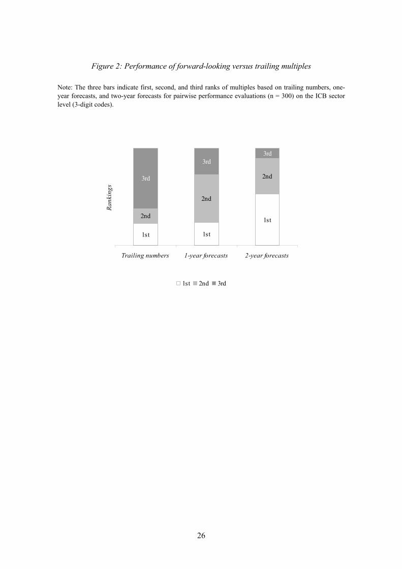
To visualize the performance of forward-looking versus trailing multiples, Figure 2

provides a bar chart containing the number of first, second, and third ranks of multiples

based on trailing numbers, one-year forecasts, and two-year forecasts for pairwise per-

formance evaluations on the ICB sector level. Out of 300 comparisons, two-year fore-

casts perform best ranking first 160 times, second 108 times, and third only 32 times.

One-year forecasts reach 72 first, 146 second, and 82 third ranks. Far behind, trailing

numbers rank first only 68 times, second 46 times, and third 186 times.

In sum, the results presented in Table 6 and Figure 2 suggest the following ranking

of multiples and therewith support Hypothesis 3: Forward-looking multiples, as a group,

exhibit higher accuracy than trailing multiples. Performance increases with the forecast

horizon from one year to two years.

20

5.5 Evaluation of results

The empirical results for the European sample substantiate the economics of the com-

prehensive multiples valuation framework. It is worthwhile to validate the significance

of the results using U.S. data. The out-of-sample test confirms our findings. In fact,

even the magnitude of most results shows strong similarities.

One aspect of the results for the U.S. sample provides evidence for a phenomenon

observed by Ali & Hwang (2000): Accounting information exhibit greater value rele-

vance in U.S. equity markets than elsewhere in the world. Table 7 shows that across the

universe of equity value multiples in the study, the median absolute valuation error

(fraction of valuation errors below 15 percent) is on average 10.0 percent lower (8.9

percent higher) for the U.S. sample compared to the European sample. The obvious and

first explanation for the performance advantage of the U.S. sample is the heterogeneity

of accounting and tax regulations across Europe. A second explanation is that the de-

mand for published value relevant accounting information is higher in equity- and mar-

ket-orientated financial systems (e.g., U.S.) than in debt- and bank-orientated systems

(e.g., Germany and France). Why? Banks typically have direct access to firm informa-

tion. One might also attribute the performance advantage of U.S. markets to a supposed

higher degree of capital market efficiency.

Interestingly, the relative performance advantage reported in Table 7 is based on

four multiples: (1) The trailing P/E, (2) the one-year forward-looking P/E, (3) the two-

year forward-looking P/E, and (4) the P/B multiple. The conclusion is two-fold: First,

the popularity of the P/E and the P/B multiple among U.S. market participants has an

impact on the market price levels of U.S. stocks. Second, analysts covering U.S. stocks

produce earnings forecasts that better reflect intrinsic value generation than analysts

covering European stocks. A closer look at the results of the cross-sectional analysis of

the U.S. sample shows that entity value multiples perform slightly better in the U.S.

than they do in Europe when compared to the equivalent equity value multiples. This

amelioration lapses through the additional provision of equity value multiples. This can

be explained by the differences in consistency. The advantages of knowledge-related

and of forward-looking multiples compared to traditional and trailing multiples are

stronger in the U.S. than in Europe.

21

5.6 Time stability and limitations

Another issue concerns the time stability of the results. To evaluate the steadiness of the

accuracy pattern, we focus on eleven equity value multiples and calculate calibrated

performance indicators in each year from 1996 to 2005. In an aggregated form, Figure 3

shows the progression of the calibrated median absolute valuation errors and quartile

errors for the European sample over the horizon. The absolute and relative levels of

those performance indicators appear fairly consistent over time. One noticeable devia-

tion occurs during the years of the boom and bust of the dot-com bubble. That is, after a

decline of valuation accuracy in 1999 and 2000, we observe a reversion in 2001 and fur-

ther slightly positive adjustments in the years thereafter. Albeit this deviation, the flat

curves suggest that the overall results are robust throughout the sample period.

The dataset and sample selection impose two notable limitations on the empirical

results. The first limitation concerns the selection of the Dow Jones STOXX 600 and

the S&P 500 as the underlying indices of the study. Although they cover the majority of

the total market capitalization in Western Europe and the U.S., the number of stocks is

limited to only 600 and 500 respectively. Classifying single stocks in large cap or mid

cap, the sample entirely excludes small cap stocks. Furthermore, countries in Western

Europe and the U.S. represent developed equity markets as opposed to many countries

in emerging markets. Therefore, it is questionable, if the results can be directly trans-

ferred to small caps and emerging markets.

Limited data availability represents the second limitation. The dataset itself is

unique because the access to resources of Thomson Financial provides detailed I/B/E/S

forecasts on many value drivers beyond the typically available earnings (growth) fore-

casts. Complete forecast material, however, is still only available for the last six years

from 2000 to 2005 for the European sample and for the last three years from 2003 to

2005 for the U.S. sample respectively. Also, the dataset on R&D expenditures and am-

ortization of intangible assets for firms in science-based industries is incomplete be-

cause of non-uniform disclosure regulations in different countries and industries. The

two limitations in data availability may reduce the reliability of the results concerning

forward-looking and knowledge-related multiples.

22

6 Conclusion

This paper examines the valuation accuracy of different types of multiples in European

equity markets. We use a dataset of 600 European firms and construct a comprehensive

list of multiples for the ten-year period from 1996 to 2005. The cross-sectional analysis

assumes direct proportionality between market values and multiples. Comparable firms

are selected from the same industry based on the ICB system. Overall, the MVM in its

many variations approximate market valuations well with median absolute errors of less

than thirty percent and fractions of errors below 15 percent of higher than thirty percent

for the majority of the equity value multiple universe. In terms of relative performance,

our results show that: (1) Equity value multiples outperform entity value multiples. (2)

Knowledge-related multiples outperform traditional multiples in science-based indus-

tries. (3) Forward-looking multiples, in particular the two-year forward-looking P/E

multiple, outperform trailing multiples.

All of our results are significant in magnitude, robust to the use of different statisti-

cal performance measures, and constant over time. More importantly, the study finds

similar or even stronger results in an out-of-sample test using a dataset of 500 U.S.

firms for the same time horizon. In sum, our results extend the knowledge of the abso-

lute and relative valuation accuracy of different (types of) multiples and provide reason-

ing for the industry practice of using multiples as the standard valuation approach.

The straightforwardness of the methodology and the significance of the empirical

results make these results directly relevant to practice. There is a good indication of

which type of information the market processes in order to determine values. The study

supports the importance of knowledge-related variables in science-based industries. It

also supports the importance of earnings forecasts across all industries.

Our study opens space for further investigation in the area of corporate valuation

using multiples. We suggest an extension of the dataset for the cross-sectional analysis

to emerging markets and small firms.

23

References

Aboody, D., Lev, B.: The Value Relevance of Intangibles – The Case of Software Capi-

talization. Journal of Accounting Research 36, 161-191 (1998).

Aboody, D., Lev, B.: Information Asymmetry, R&D, and Insider Gains. Journal of Fi-

nance 55, 2747-2766 (2000).

Alford, A. W.: The Effect of the Set of Comparables on the Accuracy of the Price-

Earnings Valuation Method. Journal of Accounting Research 30, 94-108 (1992).

Ali, A. Hwang, L.-S.: Country-Specific Factors Related to Financial Reporting and the

Value Relevance of Accounting Data. Journal of Accounting Research 38, 1-21

(2000).

Baker, M. Ruback, R. S.: Estimating Industry Multiples. Working Paper, Harvard Uni-

versity (1999).

Beatty, R. P., Riffe, S. M., Thompson, R.: The Method of Comparables and Tax Court

Valuations of Private Firms – An Empirical Investigation. Accounting Horizons 13,

177-199 (1999).

Eberhart, A.C., Maxwell, W.F., Siddique, A. R.: An Examination of Long-Term Ab-

normal Stock Returns and Operating Performance Following R&D Increases. Journal

of Finance 59, 623-650 (2004).

Gilson, S. C., Hotchkiss, E. S., Ruback, R. S.: Valuation of bankrupt firms. Review of

Financial Studies 13, 43-74 (2000).

Kaplan, S. N., Ruback, R. S.: The Valuation of Cash Flow Forecasts – An Empirical

Analysis. Journal of Finance 50, 1059-1093 (1995).

Kim, M., Ritter, J. R.: Valuing IPOs. Journal of Financial Economics 53, 409-437

(1999).

Lev, B., Sougiannis, T.: The capitalization, amortization, and value-relevance of R&D.

Journal of Accounting and Economics 21, 107-138 (1996).

Lie, E., Lie, H. J.: Multiples Used to Estimate Corporate Value. Financial Analysts

Journal 58, 44-54 (2002).

24

Liu, J., Nissim, D., Thomas, J. K.: Equity Valuation Using Multiples. Journal of Ac-

counting Research 40, 135-172 (2002).

Liu, J., Nissim, D., Thomas, J. K.: Cash Flow is King? Comparing Valuations Based on

Cash Flow Versus Earnings Multiples. Financial Analyst Journal 63, forthcoming,

(2007).

Modigliani, F., Miller, M. H.: The Cost of Capital, Corporation Finance, and the Theory

of Investment. American Economic Review 48, 261-297 (1958).

Myers, S. C.: Determinants of Corporate Borrowing. Journal of Financial Economics 5,

147-175, (1977).

Myers, S. C.: The Capital Structure Puzzle. Journal of Finance 39, 575-592 (1984).

Penman, S. H.: Financial Statement Analysis and Security Valuation, 2nd edn., New

York: McGraw-Hill 2004.

Ross, S. A.: Determination of Financial Structure – The Incentive Signaling Approach.

Bell Journal of Economics 8, 23-40 (1977).

25

Figure 1: Categorization of multiples

Note: P = (stock) price / market capitalization, EV = enterprise value, SA = sales / revenues, GI = gross

income, EBITDA = earnings before interest, taxes, depreciation, and amortization, EBIT = earnings be-

fore interest and taxes, EBT = earnings before taxes / pre-tax income, E = earnings / net income available

to common shareholders, TA = total assets, IC = invested capital, B = book value of common equity,

OCF = operating cash flow, D = (ordinary cash) dividend, R&D = research & development expenditures,

AIA = amortization of intangible assets, and KC = knowledge costs = R&D + AIA. Forward-looking

multiples are based on mean consensus analysts’ forecasts for the next two years (1 = one year, 2 = two

years) provided by I/B/E/S. The multiples shown within this two dimensional categorization framework

are just a selection of the universe of possible multiples. However, any multiple can be classified within

this framework.

Accrual flowmultiples

Book valuemultiples

Cash flowmultiples

Alternativemultiples

Forward-lookingmultiples

P / SA P / TA P / OCF P / SA 1

P / GI P / IC P / D

P / (EBIT+R&D)

P / SA 2

P / EBITDA P / B

P / (EBIT+AIA)

P / EBITDA 1

P / EBIT

P / (EBIT+KC)

P / EBITDA 2

P / EBT

P / (E+R&D)

P / EBIT 1

P / E

P / (E+AIA)

P / EBIT 2P / (E+KC)

P / EBT 1

P / EBT 2

P / E 1

P / E 2

EV / SA EV / TA EV / OCF EV / (EBIT+R&D) EV / SA 1

EV / GI EV / IC EV / (EBIT+AIA) EV / SA 2

EV / EBITDA EV / (EBIT+KC) EV / EBITDA 1

EV / EBIT EV / EBITDA 2

EV / EBIT 1

EV / EBIT 2

Entity value

multiples

Equity va

lue

multiples

Traditional / trailing multiples

Accrual flowmultiples

Book valuemultiples

Cash flowmultiples

Alternativemultiples

Forward-lookingmultiples

P / SA P / TA P / OCF P / SA 1

P / GI P / IC P / D

P / (EBIT+R&D)

P / SA 2

P / EBITDA P / B

P / (EBIT+AIA)

P / EBITDA 1

P / EBIT

P / (EBIT+KC)

P / EBITDA 2

P / EBT

P / (E+R&D)

P / EBIT 1

P / E

P / (E+AIA)

P / EBIT 2P / (E+KC)

P / EBT 1

P / EBT 2

P / E 1

P / E 2

EV / SA EV / TA EV / OCF EV / (EBIT+R&D) EV / SA 1

EV / GI EV / IC EV / (EBIT+AIA) EV / SA 2

EV / EBITDA EV / (EBIT+KC) EV / EBITDA 1

EV / EBIT EV / EBITDA 2

EV / EBIT 1

EV / EBIT 2

Entity value

multiples

Equity va

lue

multiples

Traditional / trailing multiples

26

Figure 2: Performance of forward-looking versus trailing multiples

Note: The three bars indicate first, second, and third ranks of multiples based on trailing numbers, one-

year forecasts, and two-year forecasts for pairwise performance evaluations (n = 300) on the ICB sector

level (3-digit codes).

1st 1st

2nd3rd

3rd

3rd

1st2nd

2nd

Trailing numbers 1-year forecasts 2-year forecasts

Rankings

1st 2nd 3rd

27

Figure 3: Time stability of calibrated absolute valuation errors in Europe

Note: To illustrate the time stability of valuation accuracy, calibrated performance indicators (median

absolute valuation error, 1st and 3rd quartile) are calculated in each year from 1996 to 2005 for eleven

representative equity value multiples. The arithmetic mean is used for the aggregation of performance

indicators.

0.00

0.25

0.50

0.75

1.00

1.25

1.50

1.75

2.00

2.25

1996 1997 1998 1999 2000 2001 2002 2003 2004 2005

Calibra

ted valuation errors

1st quartile Median absolute valuation error 3rd quartile

28

Table 1: Sample characteristics and descriptive statistics

Panel A presents the characteristics of the European sample. From the 600 stocks within the Dow Jones

STOXX 600, eight stocks of four different firms (i.e., Fresenius (Medical Care), Heineken, Reed Elsevier,

Unilever) are excluded because these firms are listed both as holding and as subsidiary, but only one set

of accounting numbers is available for each year. Panel B presents the analysis results of the pooled sam-

ple of annual data from 1996 to 2005. Annual accounting numbers are as of the beginning of January each

year. Negative numbers are excluded.

Panel A: Sample characteristics

Underlying index Dow Jones STOXX 600

Regional coverage 17 developed countries in Western Europe

Industry classification used Industry Classification Benchmark

Stocks within the sample 592

Period covered 10 years (1996-2005)

Panel B: Descriptive statistics of the sample

Median Mean1st

quartile

3rd

quartile

Number of

observations

Sales (mio $) 3558 9750 1223 9667 5367

EBITDA (mio $) 577 1653 228 1511 4675

EBIT (mio $) 410 1213 162 1065 4850

Net income (mio $) 206 1144 86 535 4917

Total assets (mio $) 5830 38766 1974 19674 5373

Invested capital (mio $) 3777 18494 1383 10814 4101

Book value of equity (mio $) 1677 4284 661 4320 5255

Operating cash flow (mio $) 393 1364 152 1079 4178

Cash dividend paid (mio $) 85 258 35 245 4662

29

Table 2: Equity value multiples summary statistics

Note: Multiples are calculated for each firm i in year t using accounting numbers and mean consensus

analyst forecasts as of the beginning of January and market prices as of the beginning of April. Criteria

for the calculation of multiples and thus inclusion into the summary statistics are: (1) firm i is part of the

sample; (2) the market capitalization of firm i is above 200 million U.S. Dollar and the value of net debt

is positive in an individual year t ; and (3) the underlying value driver x of an individual multiple λ of

firm i in year t is positive.

Median Mean1st

quartile

3rd

quartile

Number of

observations

Accrual flow multiples

P / SA 1.1 5.4 0.6 2.2 4950

P / GI 4.4 6.9 2.5 7.8 3878

P / EBITDA 6.4 10.2 4.1 9.5 4317

P / EBIT 8.9 15.6 6.0 13.6 4493

P / EBT 11.5 18.4 8.0 17.1 4615

P / E 16.8 37.6 11.7 25.7 4566

Book value multiples

P / TA 0.6 1.2 0.3 1.2 4957

P / IC 1.0 1.6 0.6 1.9 3810

P / B 2.1 4.1 1.3 3.6 4865

Cash flow multiples

P / OCF 9.5 17.4 5.6 16.3 3909

P / D 41.5 81.4 26.8 70.4 4449

Knowledge-related multiples

P / (EBIT+R&D) 7.1 9.8 4.7 10.7 1116

P / (EBIT+AIA) 8.4 12.3 5.7 12.4 1973

P / (EBIT+KC) 6.5 8.7 4.3 9.6 1029

P / (E+R&D) 11.3 15.8 7.4 16.6 1073

P / (E+AIA) 14.1 19.6 10.0 20.2 1898

P / (E+KC) 9.9 13.3 6.6 14.5 988

Forward-looking multiples

P / SA 1 1.2 13.8 0.6 2.6 3150

P / SA 2 1.1 14.0 0.5 2.4 3146

P / EBITDA 1 6.5 23.0 4.3 9.8 2995

P / EBITDA 2 5.9 17.7 3.9 8.6 2995

P / EBIT 1 9.2 17.2 6.4 13.4 2929

P / EBIT 2 8.1 38.6 5.8 11.3 2945

P / EBT 1 10.5 14.8 7.7 14.9 3058

P / EBT 2 9.3 30.7 6.9 12.6 3128

P / E 1 15.8 31.0 11.6 22.7 3056

P / E 2 14.1 21.6 10.7 19.1 3125

Equity va

lue multiples

30

Table 3: Absolute valuation accuracy of equity value multiples

Note: Statistical measures of absolute valuation accuracy (median, mean, 1st and 3rd quartile) are based

on scaled absolute valuation errors (see equation (9)). The fraction <0.15 (<0.25) measures the proportion

of scaled absolute valuation errors below 15 percent (25 percent).

Median Mean1st

quartile

3rd

quartile

Fraction

< 0.15

Fraction

< 0.25

Accrual flow multiples

P / SA 0.4374 0.7478 0.1816 0.7656 0.2294 0.3395

P / GI 0.4000 0.6979 0.1620 0.7178 0.2464 0.3611

P / EBITDA 0.2954 0.5083 0.1224 0.5547 0.3118 0.4449

P / EBIT 0.2872 0.4942 0.1184 0.5551 0.3213 0.4618

P / EBT 0.2809 0.4801 0.1140 0.5508 0.3189 0.4650

P / E 0.2925 0.4831 0.1123 0.5610 0.3094 0.4571

Book value multiples

P / TA 0.3775 0.6696 0.1561 0.6715 0.2585 0.3818

P / IC 0.3480 0.6609 0.1364 0.6393 0.2797 0.4038

P / B 0.3729 0.5600 0.1570 0.6458 0.2566 0.3733

Cash flow multiples

P / OCF 0.3365 0.7256 0.1310 0.6712 0.3028 0.4209

P / D 0.3468 0.6255 0.1366 0.6466 0.2811 0.4005

Knowledge-related multiples

P / (EBIT+R&D) 0.2735 0.4599 0.1101 0.5294 0.3362 0.4791

P / (EBIT+AIA) 0.2714 0.4572 0.1129 0.5083 0.3310 0.4732

P / (EBIT+KC) 0.2849 0.4732 0.1027 0.5214 0.3398 0.4756

P / (E+R&D) 0.2736 0.4543 0.1171 0.5218 0.3261 0.4805

P / (E+AIA) 0.2537 0.4445 0.1003 0.4957 0.3461 0.4903

P / (E+KC) 0.2729 0.4512 0.1093 0.4989 0.3244 0.4623

Forward-looking multiples

P / SA 1 0.4376 0.7069 0.1915 0.7339 0.2241 0.3304

P / SA 2 0.4297 0.6853 0.1940 0.7107 0.2248 0.3302

P / EBITDA 1 0.2813 0.5568 0.1186 0.5504 0.3188 0.4755

P / EBITDA 2 0.2658 0.4798 0.1156 0.4981 0.3285 0.4893

P / EBIT 1 0.2628 1.9712 0.1128 0.5256 0.3346 0.4924

P / EBIT 2 0.2483 1.7225 0.0971 0.4537 0.3662 0.5222

P / EBT 1 0.2403 0.4101 0.0988 0.4675 0.3621 0.5265

P / EBT 2 0.2151 0.3348 0.0854 0.4119 0.4003 0.5580

P / E 1 0.2441 0.3649 0.0909 0.4621 0.3609 0.5152

P / E 2 0.2155 0.3168 0.0863 0.4121 0.3954 0.5635

Equity va

lue multiples

Analysis of absolute valuation errors Fractions

31

Table 4: Performance of equity value versus entity value multiples

Note: Negative numbers for the absolute (relative) difference of median valuation errors indicate that eq-

uity value multiples outperform entity value multiples. For instance, using the P/GI multiple instead of the

EV/GI multiple reduces the absolute (relative) median valuation error on average by 5.65 percentage

points (14.12 percent). Positive numbers for the absolute (relative) difference of the fraction <0.15 also

indicate that equity value multiples outperform entity value multiples. For instance, using the P/GI multi-

ple instead of the EV/GI multiple increases the fraction of valuation errors below 15 percent on average

by 1.05 percentage points in absolute terms and by 4.27 percent in relative terms. For the overall com-

parison, the average of the individual differences is taken.

Absolute

difference

Relative

difference (%)

Absolute

difference

Relative

difference (%)

Overall comparison

Equity value MP vs. Entity value MP -0.0694 -22.51% 0.0126 1.22%

Accrual flow multiples

P / SA vs. EV / SA -0.0621 -14.20% -0.0096 -4.17%

P / GI vs. EV / GI -0.0565 -14.12% 0.0105 4.27%

P / EBITDA vs. EV / EBITDA -0.0568 -19.22% -0.0033 -1.05%

P / EBIT vs. EV / EBIT -0.0705 -24.54% 0.0289 9.00%

Book value multiples

P / TA vs. EV / TA -0.0103 -2.74% 0.0018 0.71%

P / IC vs. EV / IC 0.0149 4.28% -0.0166 -5.94%

Cash flow multiples

P / CFO vs. EV / CFO -0.1076 -31.99% 0.0273 -30.28%

Knowledge-related multiples

P / (EBIT+R&D) vs. EV / (EBIT+R&D) -0.0738 -26.98% 0.0414 12.30%

P / (EBIT+AIA) vs. EV / (EBIT+AIA) -0.0351 -12.95% 0.0095 2.86%

P / (EBIT+KC) vs. EV / (EBIT+KC) -0.0325 -11.40% 0.0266 7.84%

Forward-looking multiples

P / SA 1 vs. EV / SA 1 -0.0916 -20.92% -0.0006 -0.29%

P / SA 2 vs. EV / SA 2 -0.1032 -24.03% -0.0070 -3.09%

P / EBITDA 1 vs. EV / EBITDA 1 -0.1001 -35.59% 0.0162 5.07%

P / EBITDA 2 vs. EV / EBITDA 2 -0.0899 -33.84% 0.0104 3.17%

P / EBIT 1 vs. EV / EBIT 1 -0.1334 -50.76% 0.0323 9.65%

P / EBIT 2 vs. EV / EBIT 2 -0.1023 -41.18% 0.0345 9.41%

Fraction < 0.15Median valuation errors

32

Table 5: Performance of knowledge-related versus traditional multiples

Note: Science based industries are identified on the ICB supersector level (2-digit codes) and include oil

& gas (0500), chemicals (1300), basic resources (1700), construction & materials (2300), industrial goods

& services (2700), automobiles & parts (3300), food & beverage (3500), personal & household goods

(3700), health care (4500), telecommunications (6500), utilities (7500), and technology (9500). The cal-

culation of absolute performance numbers is limited to these twelve industries.

Median

error

Fraction

< 0.15

Median

error

Fraction

< 0.15

Median

error

Fraction

< 0.15

Traditional accrual flow multiples

P / SA 0.4603 0.1995 6 6 12 12

P / GI 0.4406 0.2111 5 5 11 11

P / EBITDA 0.3280 0.2668 4 4 10 10

P / EBIT 0.3100 0.2962 1 2 7 7

P / EBT 0.3138 0.2989 3 1 9 6

P / E 0.3129 0.2928 2 3 8 8

Knowledge-related multiples

P / (EBIT+R&D) 0.2980 0.3114 5 4 5 4

P / (EBIT+AIA) 0.3018 0.2819 6 6 6 9

P / (EBIT+KC) 0.2962 0.3135 3 3 3 3

P / (E+R&D) 0.2807 0.3153 1 2 1 2

P / (E+AIA) 0.2974 0.3077 4 5 4 5

P / (E+KC) 0.2828 0.3252 2 1 2 1

Composite ranking of both

multiple typesAbsolute performance

Rankings within the

same multiple type

33

Table 6: Performance of forward-looking versus trailing multiples

Note: Negative numbers for the absolute (relative) difference of median valuation errors indicate that

forward-looking multiples outperform trailing multiples. For instance, using the P/E1 multiple instead of

the P/E multiple reduces the absolute (relative) median valuation error on average by 4.84 percentage

points (16.53 percent). Positive numbers for the absolute (relative) difference of the fraction <0.15 also

indicate that forward-looking multiples outperform trailing multiples. For instance, using the P/E1 multi-

ple instead of the P/E multiple increases the fraction of valuation errors below 15 percent on average by

5.15 percentage points in absolute terms and by 16.63 percent in relative terms. For the overall compari-

son, the average of the individual differences is taken.

Absolute

difference

Relative

difference (%)

Absolute

difference

Relative

difference (%)

Overall comparison

1-year forecasts vs. Trailing numbers -0.0254 -8.84% 0.0219 6.85%

2-year forecasts vs. Trailing numbers -0.0438 -15.02% 0.0449 14.13%

2-year forecasts vs. 1-year forecasts -0.0184 -7.01% 0.0229 6.58%

Sales

P / SA 1 vs. P / SA 0.0002 0.04% -0.0053 -2.31%

P / SA 2 vs. P / SA -0.0077 -1.77% -0.0046 -2.01%

P / SA 2 vs. P / SA 1 -0.0079 -1.81% 0.0007 0.30%

EBITDA

P / EBITDA 1 vs. P / EBITDA -0.0141 -4.76% 0.0070 2.26%

P / EBITDA 2 vs. P / EBITDA -0.0296 -10.02% 0.0167 5.36%

P / EBITDA 2 vs. P / EBITDA 1 -0.0155 -5.52% 0.0097 3.03%

EBIT

P / EBIT 1 vs. P / EBIT -0.0244 -8.49% 0.0133 4.14%

P / EBIT 2 vs. P / EBIT -0.0389 -13.54% 0.0449 13.96%

P / EBIT 2 vs. P / EBIT 1 -0.0145 -5.52% 0.0316 9.43%

EBT

P / EBT 1 vs. P / EBT -0.0406 -14.45% 0.0432 13.54%

P / EBT 2 vs. P / EBT -0.0658 -23.42% 0.0814 25.53%

P / EBT 2 vs. P / EBT 1 -0.0252 -10.49% 0.0382 10.56%

Earnings

P / E 1 vs. P / E -0.0484 -16.53% 0.0515 16.63%

P / E 2 vs. P / E -0.0770 -26.32% 0.0860 27.78%

P / E 2 vs. P / E 1 -0.0286 -11.73% 0.0345 9.56%

Median valuation error Fraction < 0.15

34

Table 7: Comparison of valuation accuracy in European and U.S. equity markets

Note: Negative numbers for the absolute (relative) difference of median valuation errors indicate that U.S.

data yields more accurate valuations than European data. For instance, using U.S. data instead of Euro-

pean data for the P/SA multiple reduces the absolute (relative) median valuation error on average by 3.87

percentage points (9.72 percent). Positive numbers for the absolute (relative) difference of the fraction

<0.15 also indicate that U.S. data yields more accurate valuations than European data. For instance, using

U.S. data instead of European data for the P/SA multiple increases the fraction of valuation errors below

15 percent on average by 2.62 percentage points in absolute terms and by 10.24 percent in relative terms.

For the overall comparison, the average of the individual differences is taken.

Absolute

difference

Relative

difference (%)

Absolute

difference

Relative

difference (%)

Overall comparison

U.S. vs. Europe -0.0233 -10.01% 0.0345 8.87%

Accrual flow multiples

P / SA U.S. vs. Europe -0.0387 -9.72% 0.0262 10.24%

P / GI U.S. vs. Europe -0.0498 -14.23% 0.0257 9.45%

P / EBITDA U.S. vs. Europe -0.0022 -0.75% 0.0060 1.89%

P / EBIT U.S. vs. Europe -0.0113 -4.09% 0.0143 4.25%

P / EBT U.S. vs. Europe -0.0172 -6.52% 0.0324 9.23%

P / E U.S. vs. Europe -0.0442 -17.78% 0.0490 13.66%

Book value multiples

P / TA U.S. vs. Europe 0.0174 4.40% 0.0009 0.36%

P / IC U.S. vs. Europe 0.0303 8.01% -0.0089 -3.29%

P / B U.S. vs. Europe -0.0593 -18.92% 0.0605 19.08%

Cash flow multiples

P / OCF U.S. vs. Europe -0.0139 -4.32% -0.0041 -1.38%

P / D U.S. vs. Europe 0.0422 10.85% 0.0095 3.27%

Knowledge-related multiples

P / (EBIT+R&D) U.S. vs. Europe 0.0025 0.91% -0.0029 -0.88%

P / (EBIT+AIA) U.S. vs. Europe -0.0077 -2.92% 0.0065 1.94%

P / (EBIT+KC) U.S. vs. Europe -0.0116 -4.23% 0.0044 1.27%

P / (E+R&D) U.S. vs. Europe -0.0111 -4.22% 0.0034 1.04%

P / (E+AIA) U.S. vs. Europe -0.0162 -6.84% 0.0334 8.80%

P / (E+KC) U.S. vs. Europe -0.0087 -3.30% -0.0026 -0.80%

Forward-looking multiples

P / SA 1 U.S. vs. Europe -0.0766 -21.21% 0.0501 18.28%

P / SA 2 U.S. vs. Europe -0.0676 -18.68% 0.0401 15.12%

P / EBITDA 1 U.S. vs. Europe -0.0274 -10.79% 0.0470 12.85%

P / EBITDA 2 U.S. vs. Europe -0.0265 -11.09% 0.0726 18.10%

P / EBIT 1 U.S. vs. Europe -0.0160 -6.47% 0.0538 13.85%

P / EBIT 2 U.S. vs. Europe -0.0278 -12.58% 0.0520 12.44%

P / EBT 1 U.S. vs. Europe -0.0134 -5.91% 0.0162 4.27%

P / EBT 2 U.S. vs. Europe -0.0270 -14.34% 0.0391 8.90%

P / E 1 U.S. vs. Europe -0.0732 -42.79% 0.1408 28.06%

P / E 2 U.S. vs. Europe -0.0743 -52.64% 0.1665 29.64%

Median valuation error Fraction < 0.15