multiplicity one theorems for generalized· gelfand-graev
TRANSCRIPT

Advanced .Studies in Pure Mathematics 14, 1988 Representations of Lie Groups, Kyoto, Hiroshima, 1986 pp. 31-121
Multiplicity One Theorems for Generalized· Gelfand-Graev Representations of Semisimple Lie Groups and
Whittaker Models for the Discrete Series
Hiroshi Yamashita
Contents
§ 0. Introduction
Part I. Multiplicity one theorems for generalized Gelfand-Graev rep-resentations
§ 1. Generalized Gelfand-Graev representations (GGGRs) § 2. Sufficient conditions for multiplicity free property § 3. Spaces of Whittaker distributions § 4. Quasi-elementary Whittaker distributions on Bruhat cells § 5. Important types of GGGRs and their finite multiplicity property § 6. Multiplicity one theorems for reduced GGGRs
Part II. Whittaker models for the discrete series § 7. Irreducible highest weight representations and the holomorphic
discrete series § 8. § 9. § 10.
Method of highest weight vectors Preliminaries for determination of highest weight vectors Determination of highest weight vectors (Step I) : Case of C ~ -induced GGGRs
§ 11. Determination of highest weight vectors (Step II): Case of unitarily induced GGGRs
§ 12. Whittaker models for the holomorphic discrete series and irreducible highest weight representations
References
§ O. Introduction
The idea of induced representation goes way back to G. Frobenius and I. Schur, and it has been always playing central and indispensable
Received March 23, 1987.

32 H. Yamashita
roles in the theory of group representations. This idea contributes greatly to construct irreducible representations. For example, every irreducible unitary representation of a simply connected nilpotent Lie group is obtained as an induced representation, and the Kirillov orbit method [16] tells us :how to construct it explicitly using polarization. Further, for semisimple · Lie groups, Langlands' classification of irreducible admissible representations relies largely (although not completely) upon the induction from parabolic subgroups (see e.g., [17, Chap. VIII]).
On the other hand, generalized Gelfand-Graev representations (abbreviated as GGGRs for short) we treat in this article are very interesting induced representations, though far from being irreducible. These GGGRs were constructed by Kawanaka ([13], [141) for reductive algebraic groups over a finite field, through the Dynkin-Kostant theory on nilpotent classes. They form a series of representations (in~uced from. certain kinds of unipotent subgroups), parametrized by nilpotent orbits in the corresponding Lie algebras. Among GGGRs, {he ( original) GelfandGraev representations ( = GGRs; cf. [29], see also Remark 1.2) correspond to regular nilpotent classes.
Kawanaka's results on GGGRs, enumerated below, show the impor-tance of these representations. ·
(1) The characters of GGGRs form a Z-basis of the space of unipotently supported virtual characters [15, 2A.3].
(2) These characters can be utilized to determine. explicitly the values of irreducible characters at the unipotent elements [14].
(3) Multiplicities in GGGRs give very nice informations through which one could classify irreducibles intrinsically. Among irreducible constituents of GGGRs, those occurring with "finite" multiplicity are especially important toward this direction. Here, multiplicity is understood to·. be "finite" if it is independen'.t of the cardinal number q of a finite field (when q is considered as a variable). See [15, 2.4J and 2.5.2] for more detail.
As pointed out in [13, 1.3.5], GGGRs can be constructed analogously for, n;dµctive algebraic groups over an archimedian or non-architnedian local field. So we define GGGRs of semisimple Lie groups (see Section 1 for the precise definition), and study them detailedly. By the above (3), multiplicities in GGGRs are of particular interest. ·· ·
From this point of view, the original GGRs have a very typical character: GGRs of quasi-split, linear semisimple Lie groups are of µil,lltipljcity. free (Shalika [29], .· see also (35~ Th. fl-.5]). Then .it is· quite i;iat,ural to, ask if GGQR,s as well as non-generalized GGRs have multiplicity free property or not. Here is a more direct motivation of Part I of this paper, and also of our earlier works [35] and [36] on finite multi-

Multiplicity One Theorems and Whittaker Models 33
plicity property. But, as shown in [34, 4.1], the GGGRs are far from being of multiplicity finite except the extreme case, case of GGRs. So, in order to recover the multiplicity free (or finite multiplicity) property, we need to consider reduced GGGRs, variants of GGGRs (see 1.2).
In this direction, we have shown in [36] that finite multiplicity property is actually regained for some important types of reduced GGGRs. We now recall the construction of such (reduced) GGGRs and explain our finite multiplicity theorems. (For all of the facts mentioned below, consult [36] or its short summary given in Section 5 and 9.3 of this paper.)
Let G be a connected simple Lie group with finite center, and g its Lie algebra. Denote by Ka maximal compact subgroup of G. Assume that G/K carries a structure of hermitian symmetric space. We put I= rank(G/K). Let G=KApNm be an Iwasawa decomposition of G. Then, there exists an at most two step nilpotent Lie subgroup N~Nm, canonically diffeomorphic to the Silov boundary of Siegel domain which realizes G/K. Let P be the normalizer of Nin G. Then Pis a maximal parabolic subgroup of G containing N as its unipotent radical, and so P admits a Levi decomposition P = LN = L ~ N. The Levi subgroup L acts on n= Lie N through the adjoint action, whence it acts also on the center On of n. Under this action, On has exactly (/ + 1)-number of open orbits wi (O<iS:,l). Putting w;=Ad(G)w;, we thus get nilpotent Ad(G)-orbits a\~ g, 0 < i 5:, I, which are all contained in the same nilpotent class o of g0 ==:g(8)RC. Further, we obtain on g= Uo;,;;;,;i wi (disjoint union).
The GGGR I't associated with wi is an induced representation I'i= Indi{pt), where pi is an irreducible unitary representation of Non a Fock space of n/on with respect to a certain complex structure J~'. (If G/K is of tube type, then n is abelian. So, Pt is a one-dimensional representation on the Fock space C of n/on=(O).) Throughout, we will mean by Ind either C 00 -induction ( = C 00 -Ind) or unitary induction ( = L2-Ind). Unitarily induced GGGRs L2-I'i have the following important property:
(0.1) A0 ::::: EB [oo]-L2-I';, O;;,i;:,!
where Ao denotes the regular representation of G on L2( G), and [ oo] · ir means the infinite multiple of a representation ir. In particular, the orthogonal direct sum \:B;L2-I'i is quasi-equivalent to A0 •
The reduced GGGRs coming from I'i are defined in accordance with the Mackey machine for representations of semidirect product groups, as follows. Since L acts on N, it acts also on the unitary dual N of Nin the canonical way. Let Hi denote the stabilizer of the unitary equivalence class [pi] e N of Pt in L. We can see that every Pi is extended canonically

34 H. Yamashita
to an actual (not just projective) unitary representation Pt of the semidirect product subgroup H' N = H' I>< N ~ P acting on the sanie Hilbert · space. For an irreducible (unitary, in case of £2-Ind) representation c of H', the induced representation
(0.2)
is said to be a reduced GGGR coming from I',. By construction, unitary GGGR js dec:omposed into a direct integral of the corresponding reduced GGGRs.
It should be remarked that, for any 0<i-::;;;.l, (L, H') has a structure of reductive symmetric pair (at least on Lie algebra level) associated with a signature of the restricted root system of f=Lie L. Moreover, among (L, H')'s there exist precisely two cases: (say) i =0 and i = l, for which L/ Ht is riemannian, or equivalently H' is a maximal compact subgroup of L.
Our principal results in [36] say that a fairly large number of reduced GGGRs I'tCc) have finite multiplicity property. Especially, in case i =0 or /, the corresponding reduced GGGRs are all of multiplicity finite.
In the present paper, we continue the study of .above types of (reduced) GGGRs. The contents are divided into two parts: Part I and Part II. We prove in Part I that, when i =0 or /, reduced GGGRs I'lc) have further multiplicity free property under some additional (but reasonable) assumptions on (G, c). Part II is devoted to describing embeddings of certain irreducible representations of G into (reduced) GGGRs. Such an embedding is called Whittaker model.
Now let us explain in more detail the contents of each part respectively.
0.1. Multiplicity one theorems for reduced GGGRs. The beginning four sections proceed in more general setting. First
of all, we shall define GGGRs and reduced GGGRs of semisimple Lie groups in full generality (Section 1).
After that, we give, following the formulation of Benoist [2] and Kostant [18, Section 6], nice sufficient conditions for a given monomial induced representation (C""- or £2-) Indg(i:;) of a Lie group G to have multiplicity free property (Section 2, see e.g., Theorem 2.12), where C is a unitary character of a closed subgroup Q of G. These criterions require the existence of an automorphism a of G with the following property: the anti-automorphism av of G defined by aV(g)=a(g- 1) (g e G), induces the trivial action on the space of (i:, ~)-quasi-invariant (eigen) distributions on G (see Definition 2.5) in the canonical way. In case of £2-induction, the ex-

Multiplicity One Theorems and Whittaker Models 35
istence of such a a implies that the commuting algebra End0 (L2-Indg(C))' is abelian, or equivalently L2-IndZ(C) is of multiplicity free ..
Benoist [2] further gave a sufficient condition for a given automorphism of G to have the above property, in connection with a certain geometric structure on G (cf. Proposition 2.13). There, he bears in mind the case of quasi-regular representation Indg(lQ) associated with a symmetric space G/Q, with the involution a of G canonically attached to G/Q. So, the criterion of Benoist works very well for such a case ([2], [19]; cf. [6]). However, his result can not be applied directly to the case of reduced GGGRs I'i(c) which lies outside the scope of [2]. For our multiplicity one theorems, we need to investigate matters more detailedly. This is the theme of Sections 3 and 4.
Now let G be a connected semisimple Lie group with finite center. In Section 3, we introduce spaces of Whittaker distribution on G which realize G-modules induced (in the category of distributions) from onedimensional representations of unipotent subgroups. By differentiating the group action, Whittaker distributions on any open subset of G can be defined analogously.
Section 4 is devoted to examining the supports of Whittaker distributions in connection with various kinds of Bruhat decompositions of G. More precisely, generalizing the technique of [29] and [34], we estimate supports of quasi-elementary Whittaker distributions on certain open dense subsets C,~G with supports contained in Bruhat cells G,cc, which are closed in C, and of lower dimension in general. (See 3.2 for the precise definition of C, and G,.) Here, an eigendistribution of the Casimir operator L0 is called quasi-elementary. To get the estimation, we proceed as follows. Let T be such a Whittaker distribution and take z e G. from its support. In a sufficiently small neighbourhood of z, T can be expressed uniquely as a finite linear combination of transversal derivatives of distributions on G,. Calculating l 0 T, we get the same kind of expression of L 0 T. Since Tis quasi-elementary, these two expressions coincide up to scalar multiples. This produces our estimation for the support of T (Theorem 4:2).
Returning to our original objects, we apply in 6.1 this estimation to the case of GGGRs I't· Then we can show that, if i =0 or/, any quasielementary Whittaker distribution on the whole G corresponding to I', is uniquely determined by its restriction to an open Bruhat cell (Theorem· 6.5). This means the non-existence of such type of distributions with "singular supports". This is somewhat similar to the following well;. known fact due to Harish-Chandra (cf. [IO, Th. 4]): there do not exist nilpotently supported non-zero invariant eigendistributions on semisimple Lie groups. But, if i -:f= 0, l, then there may exist non-zero quasi-elementary

36 H. Yamashi:a
Whittaker distributions with singular supports. Combining the above non-existence theorem with criterions for
multiplicity free property in Section 2, we can show that our reduced GGGRs (C 00
- or L2-) I';(c) with i =0 or I, have multiplicity free property under the assumptions: (i) G/K is of tube type (or N is abelian), and (ii) c is a real valued character of the (compact) stabilizer Hi. (See Theorems 6.9 and 6.10). These are our main results of Part I.
Our results generalize, in a certain sense, the uniqueness theorem of generalized Bessel models for the symplectic group of rank 2 over a nonarchimedian local field (Novodvorskii and Piatetskii-Shapiro; [24], [25]).
0.2. Whittaker models for the discrete series. By virtue of (0.1), any irreducible constituent of the regular repre
sentation of G appears in our GGGR L2-I't for some i, 0<i<l. So in particular, each member of the discrete series of G can be embedded into some L2-I'i. Thus there naturally arises an interesting problem: Describe Whittaker models ( = embeddings) for the discrete series into GGGRs I't·
In Part II, we settle this problem for the holomorphic discrete series by the method of highest weight vectors (explained below). This method enables us to obtain a nice description of Whittaker models, more generally for any irreducible highest weight representation of G. We deal with two types of Whittaker models. One is embeddings into C 00 -induced GGGR (C 00 -Whittaker model), the other is into unitarily induced GGGR (L2-Whittaker model).
Since a highest weight module is characterized by its highest weight vector, one may obtain a fairly good description of Whittaker models by determining highest weight vectors in GGGRs. Such a vector must be K-finite, for we are concerned with admissible representations of G.
Suggested by this idea, Hashizume [11] treated a subject similar to the above C 00 -Whittaker model. But there exist some mistakes in that paper. (For example, he asserts uniqueness of Whittaker models, which is, however, not always true. See 8.1 and Remark 10.2). Nevertheless, his method of highest weight vectors is, we feel, very nice and gives the most direct and elementary way to describe Whittaker models. Furthermore, this method is applicable also for embeddings into other types of representations. For instance, we cart describe completely embeddings of irreducible highest weight respresentations of G into the (non-unitary) principal series induced from a minimal parabolic subgroup of G (although such a description has been obtained by other methods, cf. [5], [32]). In this case, embedding into the principal series is unique up to scalar multiples (Theorem 8.1). Furthermore, we can specify the para-

Multiplicity One Theorems and Whittaker Models 37
meter of the principal series into which a given highest weight mo:iule can be embedded.
Our method of highest weight vectors proceeds, in the present case, as follows.
First, we determine explicitly all the K-finite highest weight vectors in C 00 -induced GGGRs by solving a system of differential equations on G characterizing such vectors (Theorem 10.6). Second, among these highest weight vectors, those contained in the representation spaces of L2-induced GGGRs are specified through evaluation of L2-norm (Theorem 11.3). In the latter step, we utilize the classical technique of HarishChandra [9, VI], which was used to study the non-vanishing condition for the holomorphic discrete series. These two results enable us to produce descriptions of C 00
- and L2-Whittaker models: Theorems 12.6 and 12.10, respectively. Furthermore, we can describe Whittaker models in reduced GGGRs (Theorem 12.13). These three theorems are our principal results of Part II. Our results are complete for the (limit of) holomorphic discrete series.
It should be remarked that irreducible highest weight representations occur in GGGRs with at most finite multiplicity (although non-reduced GGGRs I'i are not of multiplicity finite). So, such a Whittaker model is important from the viewpoint of Kawanaka (3) (see supra).
Our result on L2-Whittaker model (Theorem 12.9) has a certain connection with Rossi-Vergne's result [28, Cor. 5.23] that describes the restriction of the holomorphic discrete series to an Iwasawa subgroup S=.ApNm~G. Precisely, one of them can be derived from the other. However, to get our Theorem 12.10 from the result in [28], one needs many things: for instance, (a) Anh reciprocity [1] (cf. [27]), (b) detailed informations for representations of the solvable Lie group S ([4], [7], [23]), and so on. (See 12.5 for more detail.) For this reason, we wanted to take a short cut and give a more direct and more elementary proof of Theorem 12.10. Our method of highest weight vectors realizes this hope satisfactorily. Moreover, our proof is independent not only of their result but also of the technique in [28].
Our result in the present paper, as well as those in the earlier article [36], would be useful to get irreducible decomposition of unitary GGGRs L2-I'i explicitly, which we hope to treat in near future.
The author expresses gratitude to Professors M. Hashizume, N. Kawanaka and Dr. H. Matumoto for kind but stimulating discussion on generalized Gelfand-Graev representation and Whittaker model. He also thanks Professors T. Hirai and T. Nomura for useful advices and constant encouragement.

38 H. Yamashita
Notation. Let G be a Lie group, and Ha closed subgroup of G. For a continuous representation t; of H acting on a Frechet space, C 00 -Indfr(t;) denotes the smooth representation of G induced from t; in C 00 -context, defined in [35, 2.1]. If t; is a unitary representation of H, we consider the unitarily induced representation also, which will be denoted by L2-IndZ.(t;) (see e.g., [35, 3.6)). Throughout this paper, we will deal with these two types of induced representations. The notation Ind (without C 00
- or L2-) will be used to mean any one of C 00 -Ind or L2-Ind.
Part I. Multiplicity one theorems for generalized Gelfand-Graev representations
§ 1. Generalized Gelfand-Graev representations (GGGRs)
To begin with, we redefine here Kawanaka's generalized GelfandGraev representations for semisimple Lie groups, after our previous paper [36) (referred. as [II] later on). These representations are main subjects of the present article. We employ the abbreviation GGGR to denote such a representation.
1.1. Definition of GGGRs ([13), [14), [II]). Let G be a connected semisimple Lie group with finite center, and g
the Lie algebra of G. G=KApNm denotes an Iwasawa decomposition of G, and g=fEBaPEBnm the corresponding decomposition of g. We take a Cartan involution 0 of G compatible with these decompositions: K = {g e G; O(g)=g} and O(a)=a- 1 for all a e AP' Let A be the root system of (g, ap). Choose a positive system A+ of A such that ltm= I:.eA+ g(aP; l), where g(ap; l) is the root space of a root A.
Let w be a non-trivial nilpotent Ad(G)-orbit in g. Using the Dynkin-Kostant theory on nilpotent classes and the Kirillov orbit method for nilpotent Lie groups, we associate to w an induced representation I'., of G, called GGGR, in the following way. (For more detail, one should consult [II, § 1).) For each nilpotent class w=;t:(O_), there exists a unique element He aP dominant with respect to A+, such that His the semisimple element of an £ll2-triplet (X, H, Y) in g containing an Xe w:
(1.1) [H, X]=2X, [H, Y]=-2Y, [X, Y]=H.
Moreover, His uniquely determined by the nilpotent Ge-orbit o=.Ge·a> in ge containing w. Here Ge is the adjoint group of.the complexification ge of g. So we express Has H(o).
Let g=EBJezg(j) 0 denote the gradation of g determined by ad H(o).

Multiplicity One Theorems and Whittaker Models 39
Put Po= EE> J;~O g(j)o, ro = g(0)o and no= EE> n:1 g(j)o• Then Po is a parabolic subalgebra of g, and +10 =( 0 EBn0 gives its Levi decomposition. Let P 0 = L 0 N0 be the corresponding decomposition on the group level. · Here P0 =N 0 (n0 ), the normalizer of n0 in G; L 0 =Z 0 (H(o)), the centralizer of H(o) in G; and N0 =exp n0 , the analytic subgroup of G with Lie algebra n •.
Take an ~(2-ttiplet (X, H(o), Y) with Xe w as above. We define a linear from X* on n0 by
(1.2) (X*, Z)=B(Z, OX) for Z e n0 ,
where Bis the Killing form of g. Let Ad* d~note the coadjoint representation of lf O on the dual space nt of n0 • Since N 0 is a simply connected nilpotent Lie group, the coadjoint orbit space n;/Ad*(N 0 )
corresponds bijectively to the unitary dual N0 of N 0 through the Kirillov map (see [II, 1.3]). Let ~x be theirreducible unitl:!,ry representation of N 0
corresponding to the orbit [X*]=Ad*(N 0)X*. One can· realize ~x explicitly as a )llonomial representation of N 0 , using a real polarization at X * e n;. A~tually, it is easily seen that, the ideal n(2)0 = EB J.: 2 g(j) 0 of n0 coincides with the radical of X*: .
n(2)0 ={Ye n0 ; ad*(Y)X*=0},
where ad*(Y)=(d/dt)Ad*(exp tY)li=o for Ye n0 • So there exists a subspace b(X) of g(l) 0 such that n(X)=b(X)EBn(2) 0 is a real polarization at X*:
X*([n(X), n(X)])=(0), - . 2 dim b(X)= dim g(l )0 •
Let 7Jx be a unitary character of N(X)=exp n(X) given as
(1.3) 7):x(exp Z)=exp r-I (X*, Z) for Z e n(X).
Then ~ x can be realized as the unitarily induced representation:
(1.4)
From this construction, ~ x is either one-dimensional or infinite-dimensional according as g(l) 0 =(0) or not.
Now consider the induced representation I'x=Indt(~x), Here, Ind means, as in our previous paper [35] (referred as [I] later on), either £2-Ind (=the unitary induction) or C"°~Ind (the C 00 -induction). The equivalence class [I' xlof I' x does not depend on a choice of X, since any of such X belongs to an Ad(L0 )-orbit in g(2)0 in common (see [II, Prop.

40 H. Yamashita
1.9)). So we may express I' x as I' .. without any confusion.
Definition 1.1. The induced representation I'.,=Indt(~x) is called the generalized Gelfand-Graev representation ( = GGGR) associated with the nilpotent class wcg.
Remark 1.2 [II, 1.5]. A real semisimple Lie algebra g contains a regular nilpotent Ad(G)-orbit if and only if g is quasi-split, that is, the centralizer m of aP in f is abelian. In such a case, the GGGRs associated with regular nilpotent classes coincide with the original Gelfand-Graev representations ( = GGRs for short), or the representations of G induced from non-degenerate unitary characters of the maximal unipotent subgroup Nm· These (unitary) GGRs are known to be of multiplicity free if G is a linear group ([29], see also [I, Th. 4.51).
1.2. Reduced GGGRs ([15, 2.5], [II, Section 2)). Contrary to the case of original' GGRs, the generalized GGGRs fail
to be of multiplicity finite in general. So, in order to reduce the infinite multiplicities in GGGRs to be finite or to be one if possible, we introduced in [II] a variant of GGGR, called reduced GGGR ( = RGGGR for short). We actually gave there finite multiplicity theorems for some important classes of RGGGRs closely related to the regular representation (see Section 5 below).
In the Part I of this paper, we shall prove that the above important types of RGGGRs, already known to be of multiplicity finite, have further multiplicity free property under some reasonable assumptions.
Now let us recall the construction of RGGGRs. Let I'.,=lndX..(c;x) (o=Gc·m, Xe w) be the GGGR associated with a nilpotent class w of g. The Levi subgroup L 0 =Z 0 (H(o)) acts on N 0 through the conjugation. Hence it acts also on the unitary dual N0 through
(1.5) /.[~]=[/-~], (l · ~)(n)=~(/- 1nl) (n e N 0 )
for l e L 0 and [,;] e N0 , where [,;] is the unitary equivalence class of a unitary representation f of N 0 • Let H 0 (X) be the stabilizer of [~x] in L 0 •
It coincides with ZL0(0X), which is known to be reductive. Then, c;x can be extended canonically to a unitary (projective, in general) representation ~x of the semidirect product subgroup S 0 (X)=H 0 (X)N 0 ~P 0 acting on the same Hilbert space. Moreover, for any case treated in later sections, such an extension ~ x can be chosen to be genuine (not just projective). So, we suppose here such a property for~ x for the sake of simplicity.

Multiplicity One Theorems and Whittaker Models 41
Definition 1.3. For an irreducible admissible (unitary, in case of L2-Ind) representation c of the reductive subgroup H 0 (X) ~ L 0 , the induced representation
(1.6)
is called the reduced generalized Gelfand-Graev representation ( = RGG GR) associated with (w, c). Here IN0 is the trivial character of N 0 •
§ 2. Sufficient conditions for multiplicity free property
In this section, we give, following Benoist [2] and Kostant [18], sufficient conditions for a monomial representation of a Lie group to have multiplicity free property. These conditions will be utilized in later sections . to prove multiplicity one theorems for reduced generalized Gelfand-Graev representations of semisimple Lie groups.
2.1. Distributions on c=-manifolds. First, we prepare here the notation and elementary facts on distribu~
tions on c=-manifolds, and then in 2.2 those on Lie groups, which will be used throughout the Part I of this paper.
Let M be a a-compact c=-manifold. Denote by <ff(M)= C 00 (M) (resp . .@(M) = C0(M)) the space of c=-functions on M (resp. such functions with compact supports) equipped with the usual Schwartz topology (see [33, p. 479]). Let .@'(M) (resp. <ff'(M)) be the topological dual space of .@(M) (resp. <ff(M)). Each element .@'(M) 3 T: .@(M)-c is said to be a distribution on M. Notice that the identical map .@(M)~<ff(M) gives a continuous embedding of .@(M) into <ff(M) with a dense image. Hence the space <ff'(M) can be identified with a subspace of .@'(M) via
<ff'(M) 3 Tr---+ Tl .@(M) e .@'(M).
Moreover, <ff'(M) coincides with the space of distributions on M with compact supports.
Now suppose that M be orientable. Then M admits a volume form QM· Let J.I denote the Borel measure on M canonically associated with QM. Then, any locally integrable function f on M (with respect to J.1) is viewed as a distribution T1 on M via
Let Diff(M) be the algebra of C 00 -differential operators on M. For any D e Diff(M), there exists a unique D* e Diff(M) (which depends on

42 H. Yamashita
the measure JJ) such that
f M (Drp) · ,[rdv = f M rp · (D*,fr )dv for all ,f,, ,fr E !!)(M).
D* is called the adjoint of D with respect to JJ. The assignment D >-+ D* gives an involutive · anti-automorphism of Diff(M). If Te !!)'(M) and D e Di:ff (M), then the functional <[, >-+ ( T, D*,f,) is also· a distribution on M, which will be denoted by DT. In this fashion, the algebra Diff(M) acts on the spaces !!)'(M) and iff'(M). Furthermore, this action, restricted to iff(M)r;;_!!)'(M), coincides with the usual differentiation of functions: DT 1 =TD 1 for De Diff(M) and/ e l(M).
2.2. Distributions on Lie groups. Now let G be a Lie group, and· g the Lie algebra of G. For sim
plicity, we always assume that G · be uniniodular. Denote by d0 (x) a Haar measure on G. Using this measure, we regard "functions" on Gas distributions, and consider the adjoints of differential ()perators.
Let g e G. For a function/ on G, we put
(2.1) (Lgf)(~)=J(g- 1x), (Rgf)(x) ·=f(xg), /(x)=f(x~ 1),
for x e G. Then the maps/ >-+L6f,f ~Rgf andf>-+ / induce topological isomorphisms of spaces $(G) and l(G). Furthermore; g~Rg and g>-+ Lg define representations of G on spaces of functions, and " gives an intertwining operator between them. These operations Lg, R 8 and v
are extended to to those on spaces iff'(G)~2}'(G) of distributions on G respectively by
(2.2)
(2.3)
(LgT, t)=(T, Lr,t),
<f, t>=<T. ,Tr),
where Tis a distribution and ,fr a test function. By differentiating representations R and L respectively, one can
associate to each Xe g, differential operators Rx and Lx on G:
(2.4) j(R,f)(g)- ~ f(g exp (IX)) I,-,,
(Lxf)(g) = -/(exp (- tX)g) 11=0• dt
for f e C(M) and g e G. Let U(gc) denote the enveloping algebra of the

Multiplicity One Theorems and Whittaker Models 43
complexification He of g. Then x ..... Lx (resp. X -Rx) extends uniquely to an isomorphism, denoted again by L (resp. R), from U(ge) onto the algebra of right (resp. left) G-invariant differential operators on G. The adjoints of Ln and Rn (D e U(ge)) are given respectively as
where v denotes the principal anti-automorphism of U(gc), or the antiautomorphism of U(ge) such that X = - X for Xe He· This notation v
is consistent with that in (2.1): (Ln/)(I)=Lvf(I), 1 = the unit element ofG.
Let T1 and T2 be two distributions on G. Suppose that either T1 or T2 has compact support. Then the convolution T1*T2 e ~'(G) of T1 with T2 can be defined by
(2.5) (t e ~(G)),
where Tlg) denotes the distribution T2 applied on functions in g e G. By definition, we see easily
(2.6) supp (T1 * 7;) ~ supp (T1) supp (I;),
where supp(T) is the support of a distribution T. So in particular, cff'(G) has a structure of algebra under convolution, and ~'(G) is a two-sided cff '( G)-module. If both T1 and I; are functions: Ti= T1 , (i = 1, 2), then the convolution is given by T1*T2 = T1,.12 with
(2.7) (g e G).
We define forge G and De U(ge), distributions og and on in cff'(G) respectively by
(2.8) (og, t>=t(g), for t e cff( G).
Through the map g-og (resp. DH-on), one can identify G (resp. U(ge)) with the group of all dirac measures (resp. the algebra of all distributions with supports at the identity). Moreover, one sees easily by definition the following relations.
(2.9) {LgT=. og*T, . RgT=. T*o~-,, LnT=on*T, RnT;;;:;:. T*ov,
(T..*T2f = f2*fl"

44 H. Yamashita
2.3. Generalized matrix coefficients for representations [18, 6.1]. Let (ir, .n") be a contiouous representation of G on a Hilbert space
.n". A vector v e .n" is called smooth if the map G 3 g i--+ ir(g )v e .n" is of class c=. The totality£= of smooth vectors for iris a ir(G)-stable, dense subspace of .n". Moreover, £= has a structure of Gf'(G)-module which extends the action G3gi-+ir(g)I£= of G~Gf'(G): for Te<b"'(G) and v e £=, the vector ir(T)v e £= is characterized by
(2.10) (ir(T)v, w)=<T(g), (ir(g)v, w)) for WE£",
where ( , ) is the inner product on .n". Notice that, for Xe g, ir(X)= ir(ox) is given by differentiating the G-action:
(2.11)
We equip £= with the usual Frechet space topology, defined by the family of seminorms {II· lb; D e U(gc)}, where II v lln = (ir(D)v, ir(D)v) 112
(v e £=). Then, for every Te Gf'(G), ir(T) gives a linear map on £=, continuous with respect to this topology.
Let£* be the continuous dual of£, which is also a Hilbert space. Denote by ir* the representation of G on £* contragredient to ir: ir*(g) =tir(g- 1) (g e G), where, for a bounded operator A on£, tA: £*-£* is its transpose. Let (£*)-= denote the continuous dual space of£=. By restricting each v* e £*, a linear functional on £, to the dense subspace£=, we can regard£*~(£*)-=. Equip(£*)-= with the Gf'(G)module structure contragredient to that on £=:
(2.12) <ir*(T)a*, w>=<a*, ir(T)w)
for Te Gf'(G) and a* e (£*)-=. On the other hand, the subspace (£*)=~£* of smooth vectors for ir* has a structure of Gf'(G)-module consistent with that on(£*)-=.
Starting from (ir*, £*) instead of (ir, £) and identifying ((ir*)*, (£*)*) with (ir, £) in the canonical way, one obtains similarly Gf'(G)modules £=~£-==((£*)*)-=. Consequently, we have the picture of G-modules:
(2.13)

Multiplicity One Theorems and Whittaker Models 45
where A-B means that Bis the dual space of A. In addition, the right and left ends are cC'(G)-modules. Suggested by (2.13), a vector in £- 00
will be called a generalized vector for rr. Now, for v e .?If and w* e .?If*, define a continuous function T;,w* on
Gby
(2.14) T;,w.(g)=<rr(g)v, w*) (g E G).
Such a function is said to be the matrix coefficient of rr associated to (v, w*). The notion of matrix coefficient can be generalized as follows.
Proposition 2.1 [18, Prop. 6.1.1.]. Let rr be any continuous representation of a Lie group G on a Hilbert space .?If, and keep to the above notations. Then one has
(1) rr(t)a E £ 00 for any a E £- 00 and any t E £&(G). (2) For a E £- 00 and b* E (£*)- 00
, define a linear functional n,b* on £&(G) by
(2.15) <T~,b*• t)=<rr(t)a, b*) Ct E £&(G)).
Then T;,b* gives a distribution on G, which is said to be the generalized matrix coefficient ( = GMC for short) of rr associated with the pair (a, b*).
We can see immediately that the GMCs have the following properties.
Lemma 2.2 [2, Lemma 4.1.1]. Let a E £- 00 and b* e (£'*)- 00• Then,
for a Te cC' (G), the GMC T;,b* satisfies the relations
(2.16)
(2.17)
(2.18)
T * T;,b.= T~,,*(T)b*,
T;,b* * T= T;<T)a,b*,
The more important property for GMC is that the equivalence class of an irreducible unitary representation is determined by the corresponding GMCs.
Proposition 2.3 [2, Lemma 4.1.2]. Let (rr, £') and (p, .fF) be two irreducible unitary representations of G, and take non-zero vectors a e £- 00
,
b* E (£'*)- 00, CE _fF- 00 and d* E (§'*)- 00
•
(I) If T;,b•= n,d•, then rr is unitarily equivalent top. (2) In such a case, let A: :Yl'~.fF be a unitary intertwining opera
tor, and A*: .fF* - :Ye'* the adjoint operator of A. Then, A(.Yf"') = .'F00
and A*((9"'*) 00 )=(£*r. So, by taking the transpose, A (resp, A*) can be

46 H. Yamashita
extended canonically to an isomorphism of rf'(G)-modules, denoted again by A (resp. A*), from ;lf- 00 onto F- 00 (resp. from (F*)- 00 onto {.ll'f*)-•). For these extended operators A and A*, one has
A(a)=,k and A*(d*)=1.b* with 1.=#=0, e C.
Now assume that G be a connected semisimple Lie group with finite center. K denotes a maximal compact subgroup of G. For such a group G, there is an important category of irreducible representations, including all the irreducible unitary representations. It consists of irreducible admissible representations. Here, a continuous Hilbert space representation 1r of G is said to be admissible if the restriction of 1r to K is unitary and has finite multiplicity property.
We wish give here a variant of Proposition 2.3 which works not only for unitary representations but also for irreducible admissible representations of G. For this purpose, we need some notation.
If (1r, .ll'f) is an admissible representation, then the space .ll'f x of Kfinite vectors for 1r consists of analytic vectors, so in particular, one has .ll'f x c .ll'f00
• This subspace .ll'f x is stable under 1r(K) and 1r(gc)- We thus get a (gc, K)-module .ll'f x· The representatiqn (1r, .ll'f) is irreducible. if and only if .ll'f xis an (algebraically) irreducible (gc, K)-module. Two admissible representations (1rt, .ll'f1,) (i = I, 2) are said to be infinitesimally equivalent if the corresponding (gc, K)-modules are equivalent. If 1r1 and 7rz are irreducible and unitary, then ir 1 is unitarily equivalent to ir 2 if and only if they are infinitesimally equivalent. (For these facts, one can consult [31, Chap. 8]. See also [I, Section 2].)
For an admissible (1r, .ll'f), .ll'f~ denotes the algebraic dual space of .ll'f x· Equip .ll'f~ with the (gc, K)-module structure contragredient to that on ;If x· Since .ll'f x is dense in .ll'f00
, we have natural inclusions of (gc, K)modules:
(2.19) { ( .ll'f*) K ~ ( .ll'f*r ~ ( .ll'f*) · 00 ~ .ll'f~,
;If K ~ .ll'foo ~ ;If· oo ~ ( .ll'f *)~.
Let A: .ll'f x ~ F x be an isomorphism of (gc, K)-modules which gives an infinitesimal equivalence between admissible representations (ir,
.ll'f) and (p, .F). Then, making use of the admissibility of 1r and p, we can define an operator A*: (F*)x-+(.ll'f*)x via
(2.20) (Av, w*)=(v, A*w*) (v e .ll'f x, w* e (F*)x).
It is easy to see that (F*)x is, as a (gc, K)-module, equivalent to (.ll'f*)x through A*. By taking the transposes of A and A*, one-thus gets (ec, K)module isomorphisms
Multiplicity One Theorems and Whittaker Models 47
(2.21) t A: ff ic~.nf"i<,
t(A*): (Jt"*)ic~(ff*)i<.
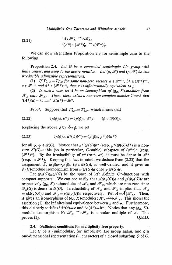
We can now strengthen Proposition 2.3 for semisimple case to the following
Proposition 2.4. Let G be a connected semisimple Lie group with finite center, and keep to the above notation. Let (11:, £) and (p, ff) be two irreducible admissible representations.
(1) Jf T~,b•=Tg,d.for some non-zero vectors a E £-=, b* E (£*)-=, c E ff-= and d* E (ff*)-=, then 11: is infinitesimally equivalent to p.
(2) In such a case, let A be an isomorphism of (gc, K)-modules from £ x onto ff x· Then, there exists a non-zero complex number J. such that t(A*)(a)=J.c and tA(d*)=J.b*.
Proof Suppose that T~,b•= Tg,d*• which means that
(2.22) <11:(rp)a, b*) = <p(rp)c, d*) (rp E .@(G)).
Replacing the above rp by ,t * rp, we get
(2.23) <11:(rp)a, 11:*( ,fr )b*) = <p(rp)c, p*( ,fr )d*)
for all rp, ,fr E 2J(G). Notice that 11:*(.@(G))b* (resp. p*(2J(G))d*) is a nonzero <!l"'(G)-stable (so in particular, G-stable) subspace of (£*) 00 (resp. (ff*) 00
). By the irreducibility of 11:* (resp. p*), it must be dense in £* (resp. in ff*). Keeping this fact in mind, we deduce from (2.23) that the assignment A; 11:(rp)a-p(rp)c (rp E .@(G)), is well-defined and it gives an @"'(G)-module isomorphism from 11:(2J(G))a onto p(.@(G))c.
Let 2Jx(G)~2J(G) be the space of left K-finite c=-functions with compact supports. We can see easily that 11:(2Jx(G))a and p(2Jx(G))c are respectively (gc, K)-submodules of £ x and ff x, which are non-zero since .@ x( G) is dense in .@( G). Irreducibility of .'Yt' x and ff x implies that £ x =11:(2Jx(G))a and ff x=p(2Jx(G))c respectively. Put A=A\ £ x· Then, A gives an isomorphism of (g0 , K)-modules: £ x~ff x· This shows the assertion (1), the infinitesimal equivalence between 11: and p. Furthermore, this A clearly satisfies tA*(a)=c and tA(d*)=b*. Notice that any (gc, K)module isomorphism V: £ x~ff x is a scalar multiple of A. This proves (2). Q.E.D.
2.4. Sufficient conditions for multiplicity free property. Let G be a (unimodular, for simplicity) Lie group again, and I; a
one-dimensional representation ( =character) of a closed subgroup Q of G.

48 H. Yamashita
Consider the induced representation (L2- or C 00-) Indg (C). An induced
representation of this form is said to be monomial. In this subsection, we give, mainly after [2], sufficient conditions for a monomial representation to have multiplicity free property in the form of four theorems. For this purpose, Propositions 2.3 and 2.4 play an essential role.
2.4.1. Case of C 00 -induced representations. First, let us consider the representation (n,, C 00 (G; C'))= C 00 -Indg (C')
induced in C 00 -context:
u e c=(G; C-), g, x e G),
where oQ is the modular function on Q with respect to a left Haar measure dQ(q) on Q: oQ(q)=dQ(xq)/dQ(x).
For a continuous Hilbert space representation (n, £') of G, let (J/t'*), 00 denote the space of generalized vectors b* e (J/t'*)-= satisfying
(2.24) for all q e Q.
Then, in view of [I, Lemma 2.2], we have
(2.25) (as vector spaces),
where the left hand side is the space of continuous G-module homomorphisms from £ 00 into C 00 (G; (). This correspondence is given as
(2.26) Hom 0 (£ 00, C 00 (G; C')) 3 B*i----+b* e (J/t'*), 00
,
b*(v)=(B*v)(I) (v e £ 00, l=the unit element of G).
So, for irreducible n, we can call dim (J/t'*), 00 the multiplicity of (n, £ 00)
inn,= C 00 -Indg ((). Now let(' be another character of a closed subgroup Q' of G. For
b* e (J/t'*), 00 and a e Jlt'·i7, the corresponding GMC T= T;,b* satisfies, in view of Lemma 2.2, the following relation.
(2.27) (q E Q, q' E Q').
Definition 2.5. An element Te !?)'( G) satisfying (2.27) is said to be a (C', (')-quasi-invariant distribution ( =(C', C")-QID for short). If such a Tis, in addition, a joint eigendistribution of Laplace operators on G: LDT= X(D)T (De Z(gc)) for some algebra homomorphism X from the center Z(gc) of U(gc) to the complex number field C, then it will be called a quasi-invariant eigendistribution ( = QIED).

Multiplicity One Theorems and Whittaker Models 49
Remark 2.6. If G is connected, any irreducible unitary representation (tr, £) of G is quasi-simple, i.e., Z(gc) acts on ;//' 00 by scalars (see e.g., [33, 4.4.1.6]). So, in such a case, any QID on G obtained as a GMC of tr is necessarily a QIED. The same holds also for irreducible admissible representations of semisimple Lie groups.
Example 2.7. Consider the case G= G, X G, (a direct product of a Lie group G, with itself), Q= Q'=diag(G, X G,)={d(g,)=(g,, g,); g, e G,}, and I;= I;'= 1 Q• the trivial character of Q. Then, Q coincides with the fixed subgroup of the involution (x, y)>---+(y, x) of G (so G/Q is a symmetric space), and G is diffeomorphic to the product G, X Q through
Hence, each right Q-invariant distribution Ton G (so is any (IQ, IQ)-QID) is identified with a T1 e !!JJ'(G,) via
for 'YI' E !!JJ( G),
where we define ,/F, e !!JJ(G,) by
Through this identification, (lQ, lQ)-QIEDs Ton G coincide with so-called invariant eigendistributions on the Lie group G,:
(2.28)
(2.29)
where g, = Lie G, and X: Z((g,)c)-+C is an algebra homomorphism. These distributions on G, have been playing an important role in the theory of group representations (e.g., the characters of irreducible admissible representations of semisimple Lie groups are QIEDs).
Using the notion of QIDs, one can give sufficient conditions for a monomial representation tr,= C 00 -Indg (I;) to be of multiplicity free.
Let Aut (G) denote the group of automorphisms of G. First,
Theorem 2.8 (cf. [2, 4.4]). Let G be any (unimodular) Lie group, and I; a character of a closed subgroup Q ~ G. Assume that there exists a a e Aut ( G) with following two properties:
(2.30) a(Q)=Q,

50 H. Yamashita
(2.31) T" = f holds for any (C, Co a)-QID Ton G,
where (T", t)=(T, ,Jr o a) (,Jr e E&(G)). Then, one has for any irreducible unitary representation (ir, .?It') of G,
(1) (dim.?lt'c,;),(dim(.?lt'*), 00 )s;;l, where 0-oo should be understood as 0. The equality holds only if ira=ir o a and ir* are unitarily equivalent.
(2) If ir* is unitarily equivalent to ira, the multiplicity of dim (.?lt'*t 00
of (ir, .?lt'00) in ir, = C 00 -Indg (C) is at most one.
Proof The proof of this theorem is same as that of [2, Prop. 4.4.1]. But we need to give it here to clarify the succeeding discussion. Suppose that (.?lt'*),00 ::;,!=(0) and .?lt'c,;::;i=(0). Take non-zero vectors b* e (.?lt'*),00
and a e .?lt'c,;, Then the GMC T;,b. gives a non-zero (C, Co a)-QID on G. By (2.31) together with (2.18), we have
Thanks to Proposition 2.3, ira and ir* are unitarily equivalent. Let A: .?lt'~.?lt'* be a unitary intertwining operator from ira to ir*. Extend A, as in Proposition 2.3 (2), to an @"'(G)-module isomorphism (ira, .?lt'-00
)~
(ir*,{.?lt'*)-00). Then, we have C(Aa) :1 b*. Once a non-zero vector a is
fixed, any b* lies in the one-dimensional subspace C(Aa)~(.?lt'*)- 00• This
proves dim (.?lt'*)Z00 = 1. Similarly one can show dim .?lt'c,; = 1. We have thus proved (1).
The assertion (2) follows from (1 ), by keeping in mind the fact that, if it'*::::'. ira, then the above intertwining operator A naturally gives rise to an isomorphism of vector spaces: .?lt'c,;::::'.(.?lt'*);00
• Q.E.D.
Remark 2.9. If G is connected, the assumption (2.31) for a can be weakened, in view of Remark 2.6 and the above proof, to the following
(2.31') T" = f for any (C, Co a)-QIED Ton G.
In semisimple case, we can yield, using Proposition 2.4 instead of Proposition 2.3, a variant of Theorem 2.8 as follows.
Theorem 2.10. Suppose that G be a connected semisimple Lie group with finite center. Consider a monomial representation ir,= C 00 -Indg (C) induced in C 00 -context. Assume the existence of a e Aut (G) with properties (2.30) and (2.31'). Then, one has for any irreducible admissible representation (ir, .?It') of G,
(1) (dim .?lt'c,;) ,(dim (.?lt'*),00 )< 1. The equailty holds only if ira and ir* are infinitesimally equivalent.

Multiplicity One Theorems and Whittaker Models 51 .
. (2) If na is equivalent to n* through a bicontinuous linear operator, then the mu/tip/city dim (.n"*)c= of (n, ,n"=) in nc does not exceed one.
The proof of this theorem is. analogous to that of Theorem 2.8, so-we omit it. ·
Let G be any Lie group again. If one can find out, for a given character i: of Q, an automorphism a of G with one more nice property ((2.32) below) in addition to (2.30) and (2.31), one can deduce the unique embedding property for irreducible representations into "'c = c=-IndZ (i:).
Theorem 2.11. Let G, Q and i: be as in Theorem 2.8. Assume that there exists a a e Aut (G) with properties (2.30), (2.31) (one can replace (2.31) by a weaker condition (2.31') if G is connected), and
(2.32)
where the bar means the complex conjugation. Then one has · ·
(2.33)
for any irreducible unitary representation (n, £") of G.
Note. Shalika utilized this criterion in the proof of multiplicity one theorem for Gelfand-Graev representations of quasi-split semisimple Lie groups [29, Th. 3.1], although he did not specify it in such fun generality as above.
Proof of Theorem 2.11. Let (n, £") be a unitary representation of G. Denote by A the conjugate linear isomorphism of Hilbert spaces from £" onto £"* such that (v, w),,.=(v, Aw),,.u• (v, we£"). This operator A commutes with the G-actions, whence it naturally gives rise to an isomorphism .n"f='.:::'.(.n"*)c=. By the assumption (2.32), one obtains .n"c.';'.:::'. (.n"*)c=. In view of (2.25) and Theorem 2.8 (1), we get (2.33) as desired.
Q.E.D.
2.4.2. Case of unitarily induced representations. Now let i: be a unitary character of Q, and consider the unitarily
induced representation (°tic, L2(G; i:))=L 2-IndZ(i:). Assume throughout that °tic is of type I. Let
(2.34) °tic'.::'. fa [m,(n)] ·n dµc(n)
denote the factor decomposition of °tic (see [I, 3.41). Here, µ, is a Borel measure on the unitary dual {; of G equipped with the Mackey Borel
52 H. Yamashita
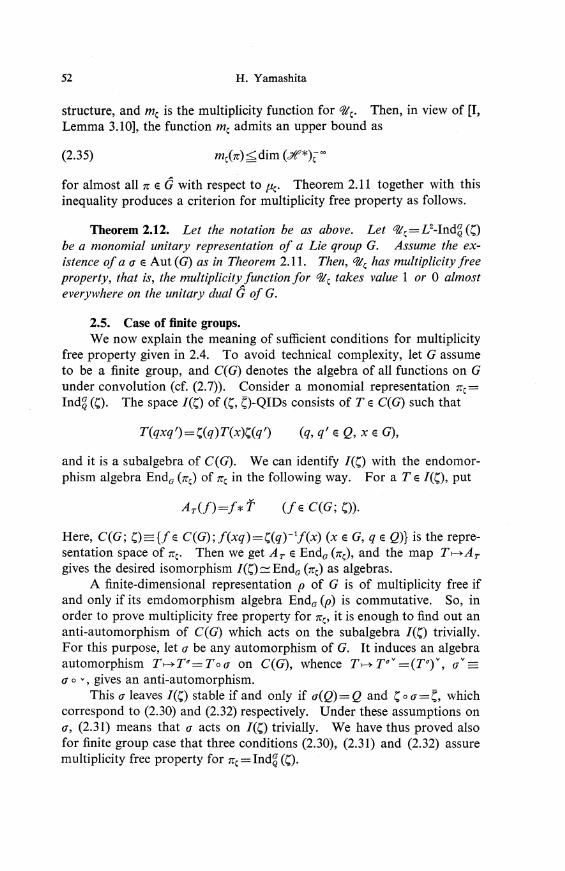
structure, and m, is the multiplicity function for %',. Then, in view of [I, Lemma 3.10], the function m, admits an upper bound as
(2.35)
for almost all 1r e G with respect to µ,. Theorem 2.11 together with this inequality produces a criterion for multiplicity free property as follows.
Theorem 2.12. Let the notation be as above. Let %',=L2-Indg (C) be a monomial unitary representation of a Lie qroup G. Assume the existence of a <1 e Aut ( G) as in Theorem 2.11. Then, 0/lr; has multiplicity free property, that is, the multiplicity function for %', takes value 1 or O almost everywhere on the unitary dual G of G.
2.5. Case of finite groups. We now explain the meaning of sufficient conditions for multiplicity
free property given in 2.4. To avoid technical complexity, let G assume to be a finite group, and C(G) denotes the algebra of all functions on G under convolution (cf. (2.7)). Consider a monomial representation 1r,=
Indg (C). The space I(C) of (C, ~)-QIDs consists of Te C(G) such that
T(qxq') =C(q)T(x)C(q') (q, q 1 E Q, X E G),
and it is a subalgebra of C(G). We can identify I(C) with the endomorphism algebra Enda (1r,) of 1rr; in the following way. For a Te I(C), put
(f e C(G; C)).
Here, C(G; C)={f e C(G);f(xq)=C(q)- 1f(x) (x e G, q e Q)} is the representation space of 1r,. Then we get AT e Enda (1r,), and the map Ti-->AT gives the desired isomorphism I(C)::::::: Enda (1r,) as algebras.
A finite-dimensional representation p of G is of multiplicity free if and only if its emdomorphism algebra Enda (p) is commutative. So, in order to prove multiplicity free property for 1r,, it is enough to find out an anti-automorphism of C(G) which acts on the subalgebra I(C) trivially. For this purpose, let a be any automorphism of G. It induces an algebra automorphism Ti-->Tq=Toa on C{G), whence Ti-->Tqv=(Tqf, av= a o v, gives an anti-automorphism.
This a leaves I(C) stable if and only if a(Q)= Q and Co a=~, which correspond to (2.30) and (2.32) respectively. Under these assumptions on <1, (2.31) means that a acts on I(C) trivially. We have thus proved also for finite group case that three conditions (2.30), (2.31) and (2.32) assure multiplicity free property for 1r, = Indg {C).

Multiplicity One Theorems and Whittaker Models 53
2.6. Benoist's condition for multiplicity free property. Let L2-Indg(i;:) be, as in 2.4, a monomial representation of a Lie
group G. Let a denote an involution of G such that a(Q) = Q. Benoist gave a sufficient condition for the property (2.31).
Proposition 2.13 [2, Prop. 3.1]. Assume the following property for a (referred as (£7!) later on): there exists a submanifold P of G such that
( i ) the multiplication m: Q X P- G is a surjective submersion. (ii) Jfp E P, thenp- 1 E P and a(p)p E Q, (iii) qPq-'=P for all q E Q, (iv) l;;(a(p)p) >O for all p E P.
Then, one gets (2.31): any (I;;, i;; o a )-QID Ton G satisfies T" = f.
This proposition together with Theorem 2.12 yields the following
Proposition 2.14 [2, Th. 5.1]. Let d/1, = L2-Indg (I;;) be a monomial unitary representation of a Lie group G. Assume that there exists an involution a of G with property (£7!). If a satisfies, in addition, ~ =( o a, then d/1/ is of multiplicity one.
Example 2.15. Let G be a connected semisimple Lie group with finite center, and i;: a real-valued character of a maximal compact subgroup K ~ G. Then, the induced representation Indf (1;;) is of multiplicity free. In fact, take as a a Cartan involution of G such that K is its fixed subgroup. Then a has property (£7!) by putting P=exp {XE g; aX = -X} and Q=K. Moreover, we have~=(=( o a, so one can apply Proposition 2.14 successfully.
Benoist's coindition works very well in case where G/Q is a symmetric space. (Notice that his emphasis in [2] is placed on the property (£1!) and on the case of exponential symmetric spaces.) But his result can not be applied directly to the case of generalized Gelfand-Graev representations. For our multiplicity one theorems, we need to investigate more closely quasi-invariant eigendistributions on semisimple Lie groups, attached to GGGRs. This is the main theme of the succeeding two sections.
§ 3. Spaces of Whittaker distributions
Hereafter, let G be a connected semisimple Lie group with finite center. In this section, we define spaces of Whittaker distributions on open subsets of G in connection with monomial representations of G induced from characters of unipotent subgroups (cf. [12], [20]). We also introduce the notion of Whittaker distributions with singular supports with respect to the Bruhat decompositions of G.

54 H .. Yamashita
If there do not exist non-zero Whittaker distributions with singular supports, then the study of the above monomial representations is simplified to a certain extent: This can be seen from Proposition 3.1. We will utilize it in later sections to prove our multiplicity one theorems.
3.1. Whittaker vectors and Whittaker distributions. Let G=KAPN"' be an Iwasawa decomposition of G, and keep to the
notation in the previous sections. Denote by 1J a character of a connected Lie subgroup N of the maximal unipotent subgroup N"'. For an irreducible admissible representation (1r, .Yf) of G, a generalized vector in (.1l'*); 00 (see (2.24)) is said to be a Whittaker vector of type (N, YJ) (see [34, Def. 1.11). Let b* e (.1l'*); 00
, *O. In view of (2.25), b* characterizes an embedding B* of the smooth representation (1r, .1l'00
) into (1r~, C 00 (G; r;)) = C 00 -Indg (YJ):
(3.1)
where T~,b.(g)=(1r(g)v, b*) (g e G) is a GMC of 1r. Furthermore, this map B* can be extended naturally to an i&"'(G)-niodule embedding J"l'-00
c:;~'(G), a,->{T;,b.) V. We thus meet with the distributions T= T;,b. (a e J"l'- 00
) on G which satisfy in view of Lemma 2.2, the following conditions:
(3.2)
(3.3)
LnT=1J(n)- 1T (n e N),
LnT=X(D)T (De Z(gc))
for some algebra homomorphism X: Z(gc)-C. This means that Tis a left YJ-QIED on G. Since N is simply connected, (3.2) is equivalent to
(3.4) for Z e n:::Lie N,
where YJ': n-c is a Lie algebra homomorphism such that YJ'(Z) = (d/dt)YJ(exp tZ) li=o·
Bearing in mind that the conditions (3.3) and (3.4) have a meaning also for distributions Ton any open subset OCG, we put
(3.5) {~'(0; YJ')={Te ~'(0); Tsatisfies (3.4)},
~'(0; Y)': X)= {Te ~'(0); T satisfies (3.3) and (3.4)}.
Each element of ~'(0; YJ') is called a YJ'-Whittaker distribution on 0. We call such a distribution X-elementary, if it lies further in the subspace ~'(0; YJ': X)~~'(0; YJ').
Among Laplace operators Ln (De Z(gc)) on G, the Casimir operator

Multiplicity One Theorems and Whittaker Models 55
L 0 , !J=the Casimir element of U(gc), plays an important role. Replacing (3.3) by a weaker condition
(3.6) for ,c e C,
we can define similarly !!))'( 0; r/, ,c), which will be called the space of ,c
quasi-elementary r/-Whittaker distributions on 0. Clearly one has
f!))'(O; r/: X)~f!))'(O; r/, ,c)~f!))'(O; r;') with K=X(Q).
Each of these spaces has a right c&''(G)-module structure under convolution.
3.2. Whittaker distributions on Bruhat cells. We now recall after [34, 2.1] the Bruhat decompositions of G. Let
Pm=MApNm with M=ZK(Ap), the centralizer of AP in K, be a minimal parabolic subgroup of G. Denote by P a parabolic subgroup of G containing Pm- Then, the unipotent radical NP of P is a normal subgroup of P contained in Nm. Putting Lp=OPnP (O=the Cartan involution), we have a Levi decomposition P=LP I>< Np. Let P=OP denote the parabolic subgroup opposite to P, then P=Lp 1>< Up with Up=.0Np.
We denote by Wthe Weyl group of (G, AP): W=M*/M with M*= NK(Ap), the normalizer of Av in K. Then, the Weyl group W(P) of (Lp, Av) is canonically identified with the subgroup (M* n Lp)/M~ W. Take a complete system WP of representatives of the coset space W/W(P). We may assume WP 3 1 =the unit element of W. Then, the Bruhat decomposition of G with respect to (Pm, P) is given as
(3.7)
wheres* is any representative of s e Win M*. Moreover, for each s E W, the double coset G, is expressed as
(3.8)
because Pm=(Nmns*Nps*-')(Pmns*Ps*- 1). Every element of G, is expressed uniquely as a product of elements of Nm ns*Nps*- 1 and s*P. G, has a structure of a normal submanifold of G diffeomorphic to (Nm n s*Nps*- 1)xP in the canonical way.
We put C,=s*NPP=s*G, (s e W). Then C, is an open dense subset of G, and it admits a decomposition
(3.9) C,=(s*Nps*- 1)s*P=(Um n s*Nps*-')(Nm n s*Nps*-')s*P,
where Um=0Nm. The right end is canonically diffeomorphic to the direct

56 H. Yamashita
product (Um n s*Nps*- 1) X Gs. So in particular, C, contains G, as a closed submanifold.
Now we indroduce the spaces of Whittaker distributions with supports contained in Bruhat double cosets. Let N, 7J=eXp7J' be as in 3.1, X E Homalg (Z(gc), C) and JC E C. For an s E WP, we set
(3.10) {W(s; 7J': X)= {Te $'(Cs; 7J': X); supp (T)~ G,},
W(s; 1)1, K)={T E $'(Cs; 1)1, K); supp (T)~G,}.
Namely, W(s; 7J': X) (resp. W(s; 7J', K)) is the space of X-elementary (resp. JC-quasi-elementary) Whittaker distributions on Cs with supports contained in G,.
If s=l, then G1 =C 1, whence W(l; 1)1 : X)=Pfi'(C1 ; 7J': X) and W(l; 1)1, K)=Pfi'(C1 ; 1)1, K). For any Te .?fi'(G; 7J1 : X), the restriction TIG 1 gives an element of W(l; 7J': X). On the other hand, if s=;i:: 1, then dim G, < dim C,=dim G. In such a case, we say that the distributions in W(s; 7J', K) (K e C) have singular supports (with respect to (Pm, Ji)).
If there does not exist any non-zero (quasi-) elementary Whittaker distribution with singular support, the study of Whittaker distributions on the whole G becomes easy to some extent.
Proposition 3.1. Under the above notation, assume that W(s; 7J': X) =(O)for alls e WP,* l. Then the restriction mapping Pfi'(G; 7J': X) 3 TTI G1 e W(l; 7J': X) is injective. The same holds also for .?fi'(G; 1)1, K) and W(l; 1)1, IC).
Proof For ans e WP, let C, be any open subset of G containing G, as a closed submanifold. Replacing C, in (3.10) by C,, we can define the space W(s; 7J': X) of X-elementary Whittaker distributions on C, with supports in G,. Take Tfrom W(s; 7J': X), and put T'=Tl(C,nCs). Since supp (T) ~ G, ~ C, n C,, T' can be extended uniquely to an element T e W(s; 7J': X). Through this assignment T- f, we get
(3.11) W(s; 7J': X)::::: W(s; 7J': X) (as vector spaces).
Now put C, = Cs U ( U ,, Gs,) for s E WP, where s' runs through the elements of WP such that dim G,, >dim Gs. Then, C, is an open dense subset of G containing G, as a closed submanifold (see [34, p. 272]), and C1 = C1• In view of (3.11), it suffices to prove the assertion for W(s; 7J': X). This is carried out exactly as in the proof of [34, Prop. 2.3].
The second assertion is proved analogously, thus we complete th proof Q.E.D

Multiplicity One Theorems and Whittaker Models 57
Bearing this proposition in mind, we shall study in the succeeding section the spaces W(s; r/, IC) (s E Wp, =:/=-1, ICE C) of quasi-elementary Whittaker distributions with singular supports.
§ 4. Quasi-elementary Whittaker distributions on Bruhat cells
We estimate in this section the supports of quasi-elementary Whittaker distributions Te W(s; r/, IC) (see 3.2) on Bruhat cells by a technique analogous to the one employed in our previous paper [34]. The main result here is Theorem 4.2. This extends, to a much more general setting, the result of Shalika [29, Prop. 2.10], which was crucial to get multiplicity one theorem for the original Gelfand-Graev representations ( = GGRs) of quasi-split semisimple Lie groups. Theorem 4.2 enables us to prove multiplicity free property not only for the GGRs but also for the generalized ones ( = GGGRs). Later, we shall utilize Theorem 4.2 to show the non-existence of non-zero quasi-elementary Whittaker distributions with singular supports, which is the key step toward our multiplicity one theorems.
4.1. Supports of distributions in W(s; 7J', ,c). Let n be a Lie subalgebra of g=Lie G. We assume throughout this
section the following two properties for n:
(4.1) f(i)
l(ii)
n is an ideal of the maximal nilpotent subalgebra
nm=LieNm,
n is stable under Ad (AP).
The condition (ii) means that n is compatible with the root space decomposition of nm: n= I::,eA+ (n n g(ap; A)), w~1ere g(ap; A) is the root space of a root A.
Example 4.1. For a nilpotent class o of gc which intersects with g, the subalgebras n(i) 0 = EB_1;,;i g(j) 0 ~nm (i~ 1) satisfy (4.1), where g= EBjez g(j) 0 is the gradation of gin 1.1.
Let r/: n-+C be a Lie algebra homomorphism. Fix a parabolic subgroup P=LPNP containing Pm, and keep to the notation in 3.2. For an s E WP and ICE C, we consider the space W(s; r/, IC) of IC-quasi-elementary 1J'-Whittaker distributions on C,=s*NPP (F={}P) with supports contained in the Bruhat coset G,=Pms*P~c •.
Let n;, denote the closed submanifold of Nm n s* N pS*- 1 consisting of n E Nm ns*Nps*- 1 such that

58 H. Yamas:1ita
(4.2) 77'(Ad (n)Z)=O for all Z e n n Ad (s*)u p,
where Up=Onp with np=LieNp, Using an argument similar to the one in [34, Section 2], we can esti
mate the supports of Whittaker distributions on Bruhat cells as follows. Its proof will be given in 4.3-4.7.
Theorem 4.2. For any s e Wp, a Whittaker distribution in W(s; 17', 1C) {.t e C) has always its support contained in D!,s*P.
This is the main result of this section, which generalizes, in a certain sense, Theorem 2.11 of [34]. There, we gave a good estimation of supports of Whittaker distributions associated with Whittaker vectors for the (degenerate) principal series. This generalization enables us to deal with Whittaker distributions coming from any irreducible representation of G.
4.2. An application of Theorem 4.2. Before proving this theorem, we give here an application.
Theorem 4.3. Let 17': nm-+C be a non-degenerate Lie algebra homomorphism of nm, i.e., 17' I g(ap; 1)$0 for any simple root l. Consider the spaces W(s; 17', 1C) (s e Wpm= W, IC e C) of quasi-elementary Whittaker distributions on Bruhat cells with respect to the pair (Pm, Pm =OP m) of minimal parabolics. Then,
(I) W(s; 17', 1C)=(O)for any S=Fl, e Wand any IC e C. (2) The restriction map {i)'(G; 17', .t) 3 T-+ Tl G1 e W(I; 17', 1C) is in
jective, where G1=NmPm is open dense in G.
Proof We see easily from the non-degeneracy of 77' that D!, is empty for any s* 1, e W. Then, the assertions follow from Proposition 3.1 and Theorem 4.2. Q.E.D.
The above theorem includes, as a special case G=GL,,., the result of Shalika [29, Prop. 2.10]. Although we state here our result for connected semisimple Lie groups for simplicity, Theorems 4.2 and 4.3 remain true for reductive Lie groups, including GLn as a special case.
Moreover, Theorem 4.3 can be used to get another proof of Corollary 2.12 of [34], in which we gave a nice (maybe best possible) upper bound for multiplicities of the most continuous principal series in GGRs.
The rest of this section is devoted to proving Theorem 4.2.
4.3. The Casimir operator Ln on C,. Until the end of this section, we fix, n, 77', P=LPNP and s=s*M e
WP~ W. For x, ye G and De U(gc), we put vx=yxy-1, v D=Ad (y)D for short.

Multiplicity One Theorems and Whittaker Models 59
For later use, we prepare here an explicit expression of the Casimir operator of G on the open dense subset C,. Let us now define vector fields a(X) (Xe •*np) and a'(Y) (Ye•*µ) on C,=(8*Np)s*P, which is canonically diffeomorphic to •*NP X P, respectively by
(4.3) {a(X), <ft= ! <ft(n' exp (tX)s* p) l,=o•
a'(Y)z</>= :i <ft(n' exp (-tY)s*p)lt=O•
for Z=n's*pe ('*Np)s*P= C, and <ft E C(C,)=C 00 (C,). Here j5 denotes the Lie algebra of P. Then, x~a(X) (resp. Y~a'(Y)) extends uniquely to an isomorphism from the enveloping algebra U((•*np)c) (resp. U(('*.p)c)) into the algebra Diff(C,) of differential operators on C,. This extension will be denoted still by a (resp. a'). By definition, a(X) commutes with a'(Y). The tangent space Tz(C,) of C, at the point z is decomposed as
(4.4) T,( c,) = ae·n p ),EBa'('*l5),.
Now assume that z=n's*p lies in the closed submanifold G,=(Nm n s*Np)s*P, or equivalently n' E Nm n •*Np. We put
(4.5)
where um =Onm. Then, in view of (3.9) one gets
(4.6) T,( C,)=a(f),EBT,(G,),
where T,(G,)~T,(C,) is the tangent space of G, at z. The first equality in (4.6) means by definition that a(f) is transversal to G, in the sense of [29, p. 180].
We express here the Casimir operator La on C, by means of the differential operators in a(U(('*np)c)) and a'(U(('*l5)c)). For this purpose, construct the Casimir element Q e U(gc) explicitly as follows. Consider the positive definite inner product g X g 3 (X, Y) ~ - B(X, 0 Y), with the Killing form B of g. For each 2 EA+, take an orthonormal basis {Ef; I ::=;:p~d(2)=dim g(ap; 2)} of g(aP; 2) with respect to this inner product. Furthermore, {H~; 1 ~j ~ dim m} (resp. {Hk; I ::=;: k< dim aP}) denotes an orthonormal basis of m (resp. ap). Put Ff= -OEf. Then, Q e Z(gc) is expressed as
(4.7) D=2X,EA+,1;[,p;[,d(l)FfEf-"E,jH?+ L,kHl+H21;,
where 0=2- 1 "E,,EA+ d(l) ·). and, for a r E aJ, H, E aP is such that B(H, H,) = r(H) (HE ap).
We put

60 · H. Yamashita
J. ={A e A+· g(a · l)Ce} 2 , P' = and
Then one gets the following
Lemma 4.4. The Casimir operator L 0 is expressed on the open dense subset C, as
(4.8)
Lo= -2 I:1e1i,1;a;p::.dO> a(Ff)a'(Ef)-2 I:1er,,1;a;p::.d<•> a(Ef)a'(Ff)
+2 I:1er8,1;a;p::.d<•> a'(Ff)a'(Ef)
-I;,a'(H;)2
+ I:k a'(Hk)2+a'(H,),
where 1:=20- I:1e11 d(A) ·A.
Proof. For a differential operator D defined on a neighbourhood of the unit element 1 of G, we define De Diff(C.) by
(4.9) (D</J)(n's*p)=((D o Ln,-1 o R,. 11)</J)(l)
for </J e <ff(C,) and n's*p e ('*Np)s*P. (Note that n' e •*NP is an analytic function in z=n's*p e C,.) Since Q e Z(gc), one gets (L 0)-=L 0 on C,. In view of (4.7), let us calculate (LpPEP)-, ((LH1,)2)-, etc.
l l
First, assume that A e /1" By the definition of I" we have Ff e f S: •*nP (1 <p<d(l)), whence Ef e •*,13. Notice that FfEf=EfFf-H 1• Then keeping (4.3) in mind, we see easily
(4.10)
Similarly one gets
{-a(Ef)a'(Ff) (1 e I2),
(4.ll) (Lpf Ef)-= a'(Ff)a'(Ef) O e /3),
(4.12) ((LH;)2)-=a'(H;)2, ((LH.)2)-=a'(Hk)2.
The equalities (4.10)-(4.12) give the expression (4.8). Q.E.D.
4.4. Local expression of distributions with singular supports. Let T be a distribution on C, such that supp (T) s; G ,. Then, T can
be expressed locally as a finite linear combination of transversal derivatives of distributions on G,. We give here such an expression. For this purpose, fix a linear order > on a; such that A+= {A e A; A >O}. For a

Multiplicity One Theorems and Whittaker Models 61
sequence r=(r().,p)) of non-negative integers r(J., p) (). e 11, 1 :s;:p::::;d(J.)), called a multi-index later on, we put
( 4.13) pr= n' (Ffy<•,P) E U(f c)-
Here, the product n' is taken in such a way that the term (Ff:YW,p') always sits on the left of(Ff)7U,Pl if either J.'>J. or J.'=J.,p'>p. By the Poincare-Birkhoff-Witt theorem, these pr's form a basis of U(f c)-
Now take Zo=nos*JJo E G, with no E Nm n •*Np, Po E P, from the support of T. Then, according to Schwartz (cf. [29, Lemma 2.4]), there exists an open nieghbourhood O ,0 ~ C, of z0 on which T0 = Tl O 20 is expressed uniquely as
(4.14) (finite sum)
with Tr e $'(G,[z 0]), G,[z0]:====G, n O, 0• Here, for an Se $'(G,[z 0]), S denotes its trivial extension to O ,0 :
(4.15) (S, </>)=(S, ef>IG,[z0]) (<p E $(0 20 )).
Replacing 0 20 by a smaller neighbourhood of z0 if necessary, we may (and do) assume:
(i) O20 =% 0%'s*9\, where % 0 (resp. %', 9'i0) is an open neighbourhood of n0 (resp. 1, JJo) in Nm n '*Np (resp. in Um n '*Np, in P), whence G,[z0] = % 0s*tJii0,
(ii) z0 e supp (Tr) for all non-zero T/s.
Let a denote the largest integer attained by I rJ = I;r(J., p) = a for Tr°/=· 0. Then, a is independent of the choice of a neighbourhood 0, 0 with the above properties, which is said to be the transversal order of T at z0•
Now let D e U(ec) and D' e U('*,Pc)- Since a(D) and a'(D') are tangential to G, from the second equality of (4.6), the restrictions of a(D) and a'(D') onto the open subset G,[z0)~ G, naturally give rise to differential operators on G,[z0], which are denoted still by a(D') and a'(D') respectively. Note that G,=(Nm n •*Np)s*P is canonically diffeomorphic to the direct product (Nm n •* NP) X P. We will consider the action of Diff ( G ,[z0]) on $'(G,[z 0]) as in 2.1, through the measure dndp restricted to G,[z0). Here dn and dp denote respectively right Haar measures on Nm n •* Np and on P.
Now suppose that Te W(s; r/, K) for Ke C. We henceforth go to the local situation around z0 e supp (T), and study T0= Tl 0 20 instead of the global T itself.
4.5. The condition L0 T0 = ,cT0•
First, we rewrite this condition for T0 on 0. 0 to that for T/s on G,[z0].

62 H. Yamashita:
Proposition 4.S. The distribution Tr on G,[z0] coming from Te W(s; r/, K), satisfies the relation
(4.16)
for any multi-index r such that lr!=a+ l (a=the transversal order of Tat z0). Here we put
(4.17) {o[l,p]=(o1l'p,),,,p,, . .
o1l'p,=1 if(A',p')=(A,p), o1l'P,=0 otherwise.
Proof Let us calculate L 0 T0• In view of Lemma 4.4 and (4.14), one gets easily
(4.18) LoTo= -2 I::1r1=a I:ieI1,p a(PH[l,P])a'(Ef)Tr+ T',
where T' e ~'(O, 0) is such that supp (T')~G.[z 0] and that its transversal order at z0 is less than a+ 1. Here we used the following fact: Let De Diff(O, 0) be tangential to G,[z0]. If Se ~'(O, 0) such that supp (S)~G.[z 0],
then the transversal order of DS at z0 does not exceed that of S (see [29, p. 181]).
Notice the uniqueness of the local expression (4.14). Then, the condition L 0 T0=KT 0 together with (4.18) yields the desired property (4.16).
Q.ED.
4.6. The condition LzTo= -r/(Z)T 0 (Zen). Secondly, we wish to rewrite the condition of left r/-quasi-invariancy
for T0• By virtue of the assumption ( 4.1, ii), n admits a direct sum decomposition as vector space:
(4.19) n=(n n ··np)Ef)(n n •*.p).
So, we consider the following two cases separately.
4 6.1. Case of Zen n •*np, Then, Lz is tangential to G., and it commutes with a(P)'s since (n n •*np) n f = (0). Thus, LzTo= -r/(Z)T 0
is equivalent to
LzTr= -r/(Z)Tr for all r.
4.6.2. Case of Z e n n •*.p. In this case, Lz does not in general commute with the transversal differential operators a(P), so we need to calculate brackets of these two types of differential operators. For this purpose, we return to the global situation on C, for a while.
For a differential operator Don a neighbourhood of 1 e G, we put

Multiplicity One Theorems and Whittaker Models 63
(4.20) (</> E <ff(C~)),
where Z=n·U·S*·p=nus*pwith n E Nmn•'Np, UE umn•*Np and .PE Ji. Then Dt gives a differential operator on c.. (Compare with jj in (4.9).) Bearing the assumption (4.1, i) in mind, we see easily that the condition (3.4) for Tis equivalent to
(4.21) (Lz)tT= -,JrzT (Zen),
where tz e C(C.) is defined by
(4.22) ,Jrz(Z)=r;'("Z) for z=nus* p e C,.
Now let Q denote the ring of polynomial functions on f, and Q+ the maximal ideal of Q consisting of h e Q without constant term. Identifying f with Um n •*NP through the exponential mapping, we regard each h e Q as a function on the nilpotent Lie group Um n •*NP. Further, we extend each It to a c~-function on C,=(Nm n •*N;)(Um n •*Np)s*Ji via C, :> nus*p .-h(u), which will be denoted still by h for simplicity.
Under these notations, one gets
Lemma. 4.6. _Let Z e •*µ and Fe f. Then, the bracket of differential operators o(F) and (Lz)t is given as
(4.23)
modulo Q+o(•*np)EBQ+o'(•*µ)~Diff(C,), where (L[F,z1)- is as in (4.9).
Proof Fix a basis (Z,.) of g. For each integer j ~O, put ((-1) 1 /j !) . (ad V)1Z= E,. a1(V)Z,. (Ve f). Clearly, a1 is a homogeneous polynomial on f of degree j, especially a1 e Q. By definitions of D and Dt (D e Diff(G)), we see easily
(Lz)t= Ego En a'.J-(Lz,.)-, o(F)= -(LF)-.
Hence the bracket in question is calculated as
[o(F), (Lz)t]=-E1,n [(LF)"', a'.J-(LzJ-]
= - E1,n {((LF)-a'.J) ·(LzJ-+a'.J-[(LF)-, (Lz,.)-n
= - En ((LF)-an •(LzJ- (mod. Q+o(•*np)EBQ+o'('*µ)).
For the last equality, we used the facts
a1 E Q+ if j~l,
(LF)-a 1 e Q+ U (0) if j =I= I,
En a~·[(LF)-, (Lz,.)-]=[o'(Z), o(F)]=O (see 4.2).

64 H. Yamashita
From the definition of af, (Lp)-af is the constant determined by
Consequently, we deduce
as desired. Q.E.D.
We need one more lemma.
Lemma 4.7. Let De Q+a(•*np)EBQ+a'(•*p). Then, for each Se ~'(Gs), there exists a constant Cn,s e C such that DS=cv, 8 S.
Proof Lethe Q+ and Ye g=s*nPEBs*p. Case 1. If Ye •*p, then a'(Y)h=O. Hence we get h-a'(Y)S=a'(Y) ·
h · S = 0 since h e Q + is identically zero on Gs· Case 2. If Ye e=nm n •*np, then a(Y) is tangential to Gs. Hence,
h · a(Y)S=h · a(Y)S= 0. Case 3. If Ye f=umn•*np, then h-a(Y)S=a(Y)-h-s+a(Y)h-S=
(a(Y)h)(l)S. With the decomposition •*nP=eEBf in mind, we obtain the lemma.
Q.E.D.
Now let us consider the local expression (4.14) of Ton 0, 0 • From (4.21), we get the following condition on Tr e ~'(G,[z 0]).
Proposition 4.8. Let Z e n n •*p. For any multi-index r = (r(A, p)),er,, 1,.;p:a;;d(,J such that Ir\= a (=the transversal order of Tat z0), Tr satisfies
where the sum is over (A,p, A', p') with A, A' e / 1, l ~p~d(A), 1 <p'S:_d(A'). Here the constants Cirp, are determined by
(4.25) (mod. eEB'*p),
and ,frz is as in (4.21).
Proof For a multi-index r, let us calculate (Lz)ta(F7)Tr. By definitions of D and Dt (De Diff(G)), it is easy to see that (LzYTr=a'(Z)Tr, Lemmas 4.6 and 4. 7 together with this equality imply that

Multiplicity One Theorems and Whittaker Models 65
(4.26) (Lz)to(F)Tr
=o(F7)a'(Z)Tr- r;.,p r(l, p)o(F-B[l,p])(Lcz,Ff])-Tr+D'Tr,
where D' e Diff(O, 0) has the order less than Ir!- By using the expansion ( 4.25), the right hand side of ( 4.26) turns to be
o(F)o'(Z)Tr- r;l,l',p,p' C1?p,r(l, p)o(Fr-B[l,p]+6[l',p'])Tr+ r:,r'l<lrlo(F')Sr'
for some Sr, e .!'d'{G,[z0]). Consequently, we have
(4.27)
with r: e .!'d'(G,[z0]) given as
(4.28) T~=o'(Z)Tr- r; C1?p,(r(l, p)+ l)Tr+aci,pJ-aci•,p'J
for any r such that lr!=a. Taking into the uniqueness of the local expression (4.14), we thus obtain the desired equality (4.24), from (4.27), (4.28) and the condition (4.21). Q.E.D.
4. 7. Proof of Theorem 4.2. Making use of the results of the subsections 4.3-4.6, we can now
prove Theorem 4.2, the main result of this section. Let Te W(s; r/, .t) and z0 e supp (T)CG,. Keep to the notation in the previous subsections. We will show that z0 necessarily lies in the subset D:, -s*P with D!, as in (4.2). In terms of the function tz on C, introduced in (4.22), this condition means that
Fix 10 e A+ such that g(ap; l 0)~n n •*up, and Po, 1 <p 0 =s;;.d(l0). We put E=Ef:. Then it suffices to show that tE(z 0)=0. This is done in the following way.
First, let us introduce a lexicographic order on the set of multiindices r as follows: r 1 >r 2 if and only if there exists a pair {l, p) such that
(i) ri(l',p')=rll',p') if either l'>l or l=l',p'>p, (ii) riei,p)>rll,p).
We put
h=max{r{l 0,p 0); lr!=a, z0 e supp{Tr)}.
Let/ denote the totality of multi-indices r = (r(l, p )) such that r{l 0, p0) = b, lr!=a and z0 e supp (Tr)- From now on, r denotes the largest element of /.

66 H. Yamashita
Applying Proposition 4.5 to r + o[i10, p 0], we get
I:,e1,,1;,;p;;;d(l) a'(EDTr +•[lo,po]-o[l,p] = 0.
From the definition of /, one has z0 $ supp (Tr+,[io,poJ-,[,,pJ) if (i!,p) ::/= (i!0, p 0). So, in a sufficiently small neighbourhood of z0 in G., there holds that
(4.29) a'(E)Tr=0.
Second, we apply Proposition 4.8 putting Z = E. Then,
(4.30) a'(E)Tr= -,frETr+ I; C;;,(r(i!, p)+ l)Tr+o[l,p]-o[l-lo,p']•
Here, the sum is over (i!, p, p') with i! e 11 + i!0, 1 < p;;;; dO), 1 < p' < d(i!- i10), and the coefficients C;f: are defined by
(4.31)
Let us investigate each term in the summand of (4.31) separately.
Case 1. If (i!-ilo,P')::/=(i! 0,p 0), then (r+o[i!,p]-o[il-ilo,P']) Oo,Po) =rOo,Po)=b and r +o[i!, p]-o[i!-ilo,P']>r. By the maximality ofr e /, we obtain
Tr +•[l,p]-o[l-lo,p'J = 0 near z0 e supp (Tr)-
Case 2. Assume (i!- i!0, p') = Oo, p 0), or equivalently i! = 2i!0 and p' = Po· In this case we have for any 1-:::;;.p<d(i!),
0=B([E, E], Ff)=B(E, [E, Ff])
= I;p" C7,,B(E, Ff;')= C;?.,
because B(E, F{;')=B(Efi, Ff;')=op",po (Kronecker's o). , (4.29) and (4.30) together with the results of above two cases imply
that ,frETr=0 near z 0 e supp (Tr)- Consequently, we deduce ifrE(z0)=0, which completes the proof of Theorem 4.2. Q.E.D.
§ 5. Important types of generalized Gelfand-Graev representations and their finite multiplicity property
In this section, we first construct after [II] important classes of generalized Gelfand-Graev representations ( = GGGRs) closely related with the regular representation. Then we quote from that paper finite multiplicity theorems for reduced GGGRs coming from these important GGGRs

Multiplicity One Theorems and Whittaker Models 67
under the names of Theorems 5.4 and 5.5. These theorems are, in a sense, analogous to Harish-Chandra's finite multiplicity theorem for induced representations Ind~ (-r) (-re K.). We shall clarify in 5.4 the similarity between them.
In the succeeding sections, we shall concentrate on these (reduced) GGGRs. To be more precise, we give in Section 6 multiplicity one theorems for reduced GGGRs, and Part II (Sections 7-12) is devoted to describing embeddings of irreducible highest weight representations into GGGRs.
5.1. Simple Lie groups of hermitian type. Let G be a connected non-compact simple Lie group with finite
center. Hereafter, we always assume that G/ K carries a structure of hermitian symmetric space, where K is a maximal compact subgroup of G. We recall here after [II, 3.1] refined structure theorems due to Moore, for such a simple Lie group G and its Lie algebra g, which will be heavily utilized from Section 6 onward.
Let g=fEBp, f=LieK, be a Cartan decomposition of g, and 0 the corresponding Cartan involution of G. The given G-invariant complex structure on G/K naturally gives rise to an Ad (K)-invariant complex structure J on p, which can be expressed as J = ad (Z0) Ip for a uniquely determined central element Z0 of t (Note that the center of f is onedimensional under the above assumption on G.) Extending J to a linear map on Pc by complex linearity, we put P± ={Xe Pc; JX= ±-l=TX}. Then, g0 admits the decomposition
(5.1)
such that [fc, P±]~p±, [P+, p+J=[p_, p_]=(O). Let± be a maximal abelian subalgebra oft Then it is also a Cartan
subalgebra of g. Denote by 2 the root system of (gc, ±c)- Let 2 1 (resp. 2v) be the subset of compact (resp. non-compact) roots in 2:
where gc(±0 ; r) is the root space of are 2. Then we have 2=2 1 U 2 9
(disjoint union). We can take a positive system 2+ of 2 consistent with the decomposition (5.1) in the following sense:
(5.2) P±=EBrEI:gc(±c; ±r) with 2;=2+ n2v·
For each re 2, select a non-zero vector Xr e g0(±c; r) such as
(5.3) Xr-X-r, ,f=T(Xr+X-r) e fEf),f=Tp, [Xr, X_r]=H;,
where H;=Hr/2r(H 7) with Hr e ,1=1± determined by B(H, H 7)=r(H) for

68 H. Y amasliita
He tc (B=the Killing form of 9c), A root r is said to be strongly orthogonal to f3 e I if r ± f3 $ I U (0).
Construct a maximal family (r,, r2, • • ·, r1) of mutually strongly orthogonal roots in I: inductively as follows: for each k, rk is the largest root in I: strongly orthogonal to rk+i, .. ·, r1, where we consider a linear order on ~t* which determines the positive system I+. Now we set
(5.4)
and t+ will denote the orthogonal complement oft- int with respect to B. For a r e tt, put n-(r) = r I t0, the restriction of r to t0. Ifr is identi
cally zero on t0, then one may express n-(r) still as r without any confusion. So are the cases r=rk (l ~k:S:l). Let us describe the restrictions n-(r) (r e I+) by means of the orthogonal basis (r1, r2, ••• , r1) of t 0*. We put for I:S:m<k~l,
(5.5)
(5.6) Ckm={r E J;-:_-; n-(r)=(rk-rm)/2},
pkm={r E J::; n-(r)=(rk+r m)/2},
(5.7)
According to Harish-Chandra (cf. [II, Prop. 3.1)), the subsets J;-:_-and I:: of J; + are expressed respectively as
(5.8)
(5.9)
where the unions are disjoint. We put Hk=Xr.+X-r.EP for I:S:k<l. Then "E.,1?,k?,zRHk is a
maximal abelian subspace of p, so we denote it by aP. Let µ be the inner automorphism of 9c defined by
(5.10) µ=exp(: ·L,,?,k?elad(Xr.-X-r.)) (Cayley transform).
A simple calculation yields µ(Hk)=H{., whence µ(ap)=t-. Moreover, the restrictionµ It+ is identity on t+. So, the invesrse µ- 1 gives a transform on 9c carrying the complexification of the compact Cartan subalgebra t onto that of a maximally splitting one t+E[;)aP.
Let A be the root system of (g, ap). Select a positive system A+~ A consistent with J;+~J; through the Cayley transformµ: A+ U(O)=J:+ o
(µlav)U(O). We set Ak=rko(µjap) for I~k<l. Then Ok)i?,k?,i is an

Multiplicity One Theorems and Whittaker Models 69
orthogonal basis of a;. Moore's restricted root theorem tells us the following description of A+, the set II of simple roots in A+, and the Weyl group W of (g, ap) by means of the basis (i!k).
Proposition 5.1 [22, Th. 3). (1) There are two possibilities for the positive system A+ :
(CASE I) A+={Ok-i!m)/2; 1::;m<ks/}U{(i!k+i!m)/2; I<msk<l}, (CASE 11) A+={Ok-i!m)/2; 1 <m<k<l} U {i!k/2; 1 sk-;£_/}
U {(i!k + i!m)/2;1 sm<ks/}.
(2) According as (CASE I) or (CASE II) above, II is expressed as
(CASE I) II= {i!1, (i!2-i!1)/2, · · ·, (i!1-i!1-1)/2}, (CASE II) Il={i! 1/2, Oz-A 1)/2, · · ·, Oi-Ai- 1)/2}.
(3) W consists of all transforms of the form i!k~eki!a<kl• where a is an arbitrary permutation of I, 2, · · ·, !, and ek = ± 1. So, W is identified canonically with the semidirect product group 6it><. (Z/2Z)1. Here, the action of the symmetric group 6 1 of degree I on (Z/2Z)1::::: {I, -1 }1 is given as a·(ei, e2, · · ·, e1)=(e,-1(i), e,-1<zJ, · · ·, e,-•(tl).
The (CASE I) happens if and only if G/ K is holomorphically equivalent to a tube domain. So are exactly the cases g:::::§u(/, /), §lJ(l, R), §o*(4!), §o(2, q) (/ = 2) and g of type EVIi in the sense of Cartan. On the other hand, simple Lie algebras g corresponding to non-tube type hermitian symmetric spaces are listed up as g:::::§u(p, /) (p>l), §o*(4!+2) and the exceptional Lie algebra of type EVIII.
5.2. Important types of GGGRs ri. Leto denote the nilpotent G0 -orbit in 9c through the point I:; 1;,;k;a;i Xr,
e lJ+, where Ge denotes the adjoint group of 9c· Then o intersects with g [II, Lemma 3.4). We now explain the description of Ad (G)-orbits in on g given in [II]. For this purpose, set
(5.11) (I -;£_ks/).
It is easily verified that Ek e g(ap; i!k), the root space of i!k, and that µ-1(X7.)
= ,yf=-f Ek. For O < i < !, define a nilpotent element A[i] e nm=
,I;,EA+ g(ap; A) by
(5.12)
Theorem 5.2 [II, Th. 3.13]. The intersection on g splits into (I+ 1)-

70 H. Yamashita
number of nilpotent Ad ( G)-orbits wt = Ad ( G)A[i] (0 < i ~ l) :· on g = Ua~-i~lwi.
The generalized Gelfand-Graev representations of G associated to nilpotent classes wt (0<i~l) are constructed after Definition 1.1 in the following manner. Keep to the notation in Section I. The dominant element H(o) e aP is given as
(5.13)
since (A[i], I:,:.k&L Hk, tJA[i]) is an £lf2-triplet in g for each i. One gets a gradation g=EBjezg(j), g(j)=g(j) 0 , by ad H(o) such as
(5.14) jg(0)=m.EBapEB(EB,:.m#:.i g(ap; (Ak~lm)/2)),
g(l)= I:1:.k:.i g(ap; lk/2) (possibly (0)),
g(2) = L31:.m&k:.i g(ap; (lk + lm)/2),
g(j)=(0) if ij 1>3, g(j)=tJg(-j) (j E Z),
where m is the centralizer of aP in f. The parabolic subalgebra Vo= EBn:o g(j) is maximal, and Vo= fEBn with f =g(0), n=n 0 =g(l)E8g(2), gives its Levi decomposition. Let P=LN with L=PntJP and N 7 exp n, be the corresponding decomposition of the parabolic subgroup P=P 0 with Lie algebra j:)0 • Then, N is an at most two-step nilpotent Lie group, and it is canonically diffeomorphic to the Silov boundary of Siegel domain which realizes G/K. Moreover, N is abelian if and only if G/K is of tube type. This is exactly the (CASE I) of Proposition 5.1.
For each i, let <;';=<;'A[iJ denote the irreducible unitary representation of N corresponding to the coadjoint N-orbit through A[i]* e n*, where (A[i]*, Z)=B(Z, tJA[i]) (Zen). Then, the GGGR I';=I'.,, associated with wt is defined to be
(5.15)
These GGGRs have the following important property.
Theorem 5.3 [II, Th. 4.2]. The left regular representation (10 , L2(G)) of G splits into an orthogonal direct sum of the infinite multiples of unitary GGGRs L2-I';: l 0 :=EB0;a;t&L [oo]-L2-I';- In particular, the direct sum EBt L 2-I't is quasi-equivalent to 10 •
Now let us construct after Definition 1.3, reduced GGGRs ( = RGGGRs) coming from these GGGRs. We denote by Hi the stabilizer of the unitary equivalence class [,;';] e Nin the Levi subgroup L. Thanks

Multiplicity One Theorems and Whittaker Models 71
to [II, Th.4.6], ea.ch ~. can be extended canonically to an actual .(not just projective) unitary representation ~. of the semidirect product,group HiN =Ht ix. N~P, acting on the same Hilbert space. For an irreducible (unitary, in case of unitary induction) representation c of Hi, the RGGGR I'.(c)=I'.,ic) associated to (mi, c) is defined to be
.. (5.16) I'.(c)=Indi,N(c®~J with c=c®lN.
We now recall reductive symmetric pair structure of (L, Ht)(at least on the Lie algebra,level), which plays an important role for our study on multiplicities in RGGGRs I'i(c). For any e=(ei, e2, • • ·, e1) e {1, -1}1, define a map e from the root system A(O={(-<k--<m)/2; 1 ~m::;t=k~l} of ((, ap) to the set {1, -1} by
e(01:~-<m)/2)=ekem.
Then e gives a signature of roots in the sense of [26, Def. 1.1]. So one can construct a reductive symmetric pair ((, ij") as follows. Let 0. be a linear map on r such that
(5.17) {e{A)OX (XE g(ap; A), A E A(O),
0,(X)= OX (Xe mEf)ap).
Then 0, gives an involutive automorphism of r. We take as q• the Lie algebra of fixed points of 0 •.
,----t-. --- ,--(1-i)---PutX(i) = ( - l,. · ·, -1, 1, · · ·, l)foreachO~i~l. Byvirtueof[II,
Lemmas 2.1 and 3.5], the Lie algebra qi of Hi coincides with qz<il, Furthermore, if i=O or/, then H'=KnL, a maximal compact subgroup of L. So, in this case, the reductive symmetric pair (L, Hi) is riemannian;
5.3. Finite multiplicity theorems for RGGGRs I'ic) [II]. Thanks to the above symmetric pair structure, one can apply to
RGGGRs I'i(c) our results obtained in [I]. There, we have presented good sufficient conditions for induced representations of semisimple Lie groups to have finite multiplicity property. As a consequence, we find out, for instance, the following hereditary character of finite multiplicity property:
For an irreducible admissible representation c of Ht, the RGGGR C""-I'lc)=C""-Indi,N (c®~i) is of multiplicity finite if so is the restriction (c®~i) IM, where M =Zx(AP). (Note that Mis contained in every Hi.)
Investigating closely the multiplicities in (c®~i) IM, we have obtained

72 H; Yamashita
in [II] finite multiplicity theorems for RGGGRs I'lc) as follows. First, for C""-induced RGGGRs, we deduce
Theorem 5.4 [II, Th. 6.5]. If c is a.finite-dimensional representation of Ht, then the RGGGR C""-I'tCc) has finite multiplicity property, that is, every irreducible admissible (gc, K)-module occurs as a submodule of C""I'lc) with at most finite multiplicity.
Estimating the multiplicity function of a unitary RGGGR L2-I'tCc) by the multiplicities of irreducible admissible (gc, K)-submodules of C""I' lc ), we have the following finite multiplicity theorem for unitary RGGGRs.
Theorem 5.5 [II, Th. 6.6]. (1) If i=O or l, then all the RGGGRs L2-I'i(c) (c e (KnL)") associated with the nilpotent orbit w, have.finite multiplicity property, where (Kn Lr is the unitary dual of the compact group
KnL=H 0=H 1• Namely, if L2-I'lc):::::. f; [m,jir)]·irdµ,,.(n-) denotes the
factor decomposition (see [I, 3.4]), then the multiplicity function m,,c on G for L2-I'lc) takes.finite values almost everywhere with respect to the Borel measure dµ,, 0 •
(2) Assume that G/K is of tube type. Then, the representation L2-I' ;( c) is of multiplicity finite for any O < i < l and any finite-dimensional unitary representation c of H'.
5.4. Comparison with Harish-Chandra's finite multiplicity theorem. We now compare the above theorems for i=O or l, with Harish
Chandra's finite multiplicity theorem for Indi (r) (i- e K.). Let i=O or l. The original GGGR L2-I't is far from being of multiplicity finite except the unique case g:::::.~((2, R):::::.~u(l, l):::::.~p(l, R). (In this exceptional case, our GGGR becomes non-generalized GGRs, which is of multiplicity free). In view of [II, (4.13)], it is decomposed into a direct sum of RGGGRs as
(5.18)
Theorem 5.5(1) assures that each constituent L 2-I'tCc) has finite multiplicity property.
One can find out a same kind of phenomenon in Harish-Chandra's case. Now let G be any connected seinisimple Lie group with finite center, and K~G a maximal compact subgroup. Thanks to the Peter-Weyl theorem for compact groups, the regular representation AK of K is decomposed into irreducibles as
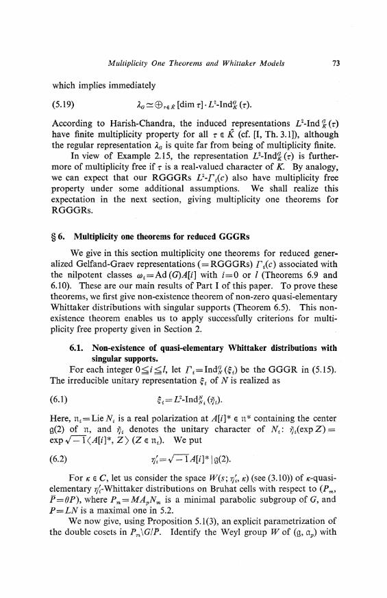
Multiplicity One Theorems and Whittaker Models 73
which implies immediately
(5.19) A0 '.:'.EB,ex [dim r-]-L2-IndHr).
According to Harish-Chandra, the induced representations £ 2-Ind CJ__ (r) have finite multiplicity property for all re K (cf. [I, Th. 3.1]), although the regular representation Ao is quite far from being of multiplicity finite.
In view of Example 2.15, the representation L2-IndCJ__ (r) is furthermore of multiplicity free if r is a real-valued character of K. By analogy, we can expect that our RGGGRs L2-I'/c) also have multiplicity free property under some additional assumptions. We shall realize this expectation in the next section, giving multiplicity one theorems for RGGGRs.
§ 6. Multiplicity one theorems for reduced GGGRs
We give in this section multiplicity one theorems for reduced generalized Gelfand-Graev representations (=RGGGRs) I'/c) associated with the nilpotent classes wi=Ad(G)A[i] with i=O or l (Theorems 6.9 and 6.10). These are our main results of Part I of this paper. To prove these theorems, we first give non-existence theorem of non-zero quasi-elementary Whittaker distributions with singular supports (Theorem 6.5). This nonexistence theorem enables us to apply successfully criterions for multi~ plicity free property given in Section 2.
6.1. Non-existence of quasi-elementary Whittaker distributions with singular supports.
For each integer O~i<l, let I'i=Ind%(.;J be the GGGR in (5.15). The irreducible unitary representation c;i of N is realized as
(6.1)
Here, ni = Lie Ni is a real polarization at A[i]* e n* containing the center g(2) of n, and i)i denotes the unitary character of Ni: r;J exp Z) = exp r-"I<A[i]*, Z) (Zeni). We put
(6.2) "f)i = r-1 A[i]* I g(2).
For IC e C, let us consider the space W(s; "f)i, IC) (see (3.10)) of 1C-quasielementary r;~-Whittaker distributions on Bruhat cells with respect to (Pm• P=OP), where Pm=MApNm is a minimal parabolic subgroup of G, and P=LN is a maximal one in 5.2.
We now give, using Proposition 5. 1(3), an explicit parametrization of the double cosets in Pm\G!P. Identify the Weyl group W of (g, aP) with

74 H. Yamashita
(Z/2Z)1 ><J 6 1• Then the subgroup W(P) corresponding to the Levi subgroup of P coincides with 6 1• Thus we can take a complete system of representatives WP in W/W(P) as Wp=(Z/2Z)1={1, -1} 1• In view of (3.7), the Bruhat decomposition of G with respect to (Pm• P) is given as
(6.3).
where e* denotes a representative of e e Win M* = N x(Ap). We wish to apply Theorem 4.2 to W(e; 1}~, K). First, let us quote a
lemnia due to Rossi and Vergne which plays an important role for our purpose. Take a pair (k, m) of integers such that 15:.m<k<l. Then we see immediately
where Em is the root vector of lm in (5.11). Note that'the root space g(ap; lk) is one-dimensional and is spanned by Ek. So, by putting
(6.4) (ad X) 2Em/2=t:;km(X)Ek with . t:;km(X) e R,
we obtain a quadratic form Ckm on g(ap; Ok-'-lm)/2).
Lemma 6.1 [28, Th. 4.10]. Under the above notation, the quadratic form Ckm is positive definite for every 15:.m <k5:. L
Making use of this lemma, let us describe, for each fixed e=(e 1, e2,
···,e 1)e{l, -1}', the closed .subset D(e,i}=D: 1~Nmn•*N ('*N= e*Ne*- 1) defined by (4.2). For this purpose, we put
Vo=(Nmn •*N) nL, Vi=Nn•*N.
Then Nm n •*N admits a semidirect product decomposition
(6.5)
Moreover we have
(6.6) V0=exp t>o with bo= I:ck,m>es g(ap; (lk-lm)/2),
where Sis the totality of pairs (k, m) such that 1 <m<k<l and (ek, em)= (1, -1). V0 is an abelian group isomorphic t:>0 through the exponential mapping, since (lk-lm)/2+(lk,-lm,)/2 ~ A for (k, m), (k', m') e S.
On the other hand, the abelian subalgebra g(2) n ••u (u=On) has an expression
(6.7) g(2) n ··u= I:mes' g(ap; lk)EBI:ck,m)eS"g(ap; (lk+lm)/2),
where
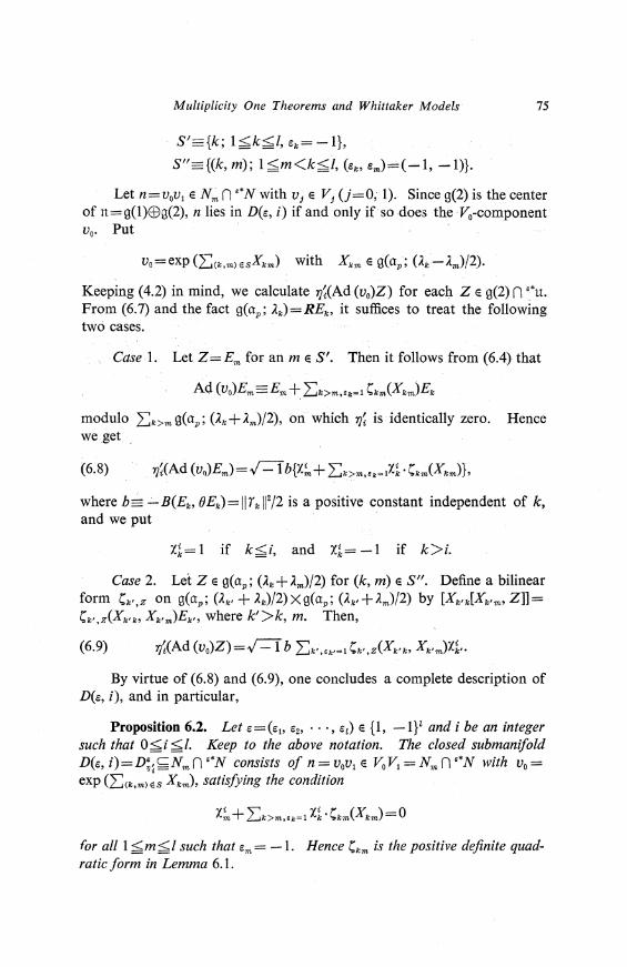
Multiplicity One Theorems and Whittaker Models 75
S'={k; 1 <k~l, ek= -1},
S"={(k, m); 1 <m<k<l, (ek, em)=(-1, -1)}.
Let n=VoV1 E Nm n •*N with vj E vj (j=O; 1). Since g(2) is the center of n=g(l)E8g(2), n lies in D(e, i) if and only if so does the V 0-component v0• Put
Vo=exp{:z::;(k,m)ESXkm) With Xkm E g(ap; (}.k-J..m)/2).
Keeping (4.2) in mind, we calculate r;~(Ad (v0)Z) for each Z e g(2) n •*u. From (6.7) and the fact g(ap; J..k)=REk, it suffices to treat the following two cases.
Case 1. Let Z=Em for an m ES'. Then it follows from (6.4) that
Ad (vo)Em==.Em + .6k>m,•k=l ,km(Xkm)Ek
modulo .6k>m g(aP; (J..k + J..m)/2), on which 7Ji is identically zero. Hence we get
where b= -B(Ek, 0Ek)=l!rkll2/2 is a positive constant independent of k, and we put
Xi= 1 if k~i, and Xi= -1 if k>i.
Case 2. Let Z e g(aP; (J..k+J..m)/2) for (k, m) ES". Define a bilinear form 'k',z on g(aP; (J..k, + J..k)/2)Xg(aP; (J..k,+J..m)/2) by [Xk'k[Xk'm, Z]]= ,k,,z(Xk'k, Xk'm)Ek,, where k'>k, m. Then,
By virtue of (6.8) and (6.9), one concludes a complete description of D(e, i), and in particular,
Proposition 6.2. Let e = (e1, e2, • • ·, e1) E { l, -1 }1 and i be an integer such that O ~ i-::;, l. Keep to the above notation. The closed submanifold D(e, i)=D:/~Nm n •*N consists of n = VoV1 E Vo V1 = Nm n •*N with Vo= exp (.6(k,m) ~s xkm), satisfying the condition
for all 1 < m ~ l such that em= -1. Hence ,km is the positive definite quadratic form in Lemma 6.1.

76 H. Yamashita
We deduce immediately from this proposition a sufficient condition fo(the set D(e, i) to be empty as follows.
Proposition 6.3. Let e and i be an in Proposition 6.2. Assume that e ::;t= 1 = (1, 1, .. , , 1 ), and denote by m. the largest integer m such that em= -1. If either i<m. or i=l, then the set D(e, i) is empty.
This proposition combined with Theorem 4.2 produces the following theorem on the non-existence of quasi-elementary Whittaker distributions onfBruhat cells.
Theorem 6.4. Let e e {1, -1} 1= WP and i be an integer such as 0<i <l. For a IC e C, consider the space W(e; 1)~, 1C) of IC-quasi-elementary 1):Whittaker distributions on C, = e* NP with supports contained in the Bruhat cell G. = P me* Pc;;;. C,. If the pair (e, i) satisfies the assumption in Proposition 6.3, then W(e; 1)~, 1C) reduces to (0). So in particular, if i=0 or l, then W(e; 1)~, IC)=(0)for all e e {l, -1} 1, ::;t=l.
Note. The second assertion turns to be false for i::;t=0, l. Actually, in case of G = Sp (2, R), the real symplectic group of rank l = 2, the spaces W(e; 1)~, 1C) (1C e C) with e=(-1, 1) and i= 1, do not reduce to (0) in general. In this case, a non-zero distribution in W(e; 1)~, 1C) can be found, for instance, as a trivial extension (to C,) of a certain Se E&'(G.) which is quasi-invariant under the action NX Pm :i (n, JJ)~LnR'JJ on E&'(G.), where Pm=0Pm•
In view of Proposition 3.1, we deduce immediately from Theorem 6.4 the following
Theorem 6.5. Assume that i=0 or l. For a IC e C, let E&'(G; 1)~, 1C) denote the space of 1C-quasi-elementary 1}~-Whittaker distributions on the whole G. Then, the restriction map
E&'(G; 1)~, IC) :l T~TINP E W(l; 7)~, IC)
is injective, where NP is open dense in G. In other words, there does not exist any non-zero quasi-elementary 1)~-Whittaker distribution with singular support with respect to (Pm, P): if Te E&'(G; 1}~, 1C) is such that supp (T)~ G\NP, then T=0.
6.2. An involution f) and its relation to QIEDs on G. Making use of this theorem and criterions for multiplicity free
property given in Section 2, we wish to give multiplicity one theorems for RGGGRs I'lc). For this purpose, we assume until the end of this sec-

Multiplicity One Theorems and Whittaker Models 77
tion that hermitian symmetric space G/K is of tube type. Under this assumption, one has the following
Lemma 6.6. (1) The element Y=:: (7rv'=T /2) · _I;1,.k,.i H;. lies in the center off, where H;. is the element oft- in (5.3).
(2) Put e": = exp Y E K. Then, the Cartan involution O is realized as the inner automorphism g1-+e":ge":-1 (g E G). In particular, e": e K is a representative of the longest element of the Wey! group W=@51 1><{I, -1} 1•
Proof By virtue of [II, Lemma 5.1], we get immediately ad (Y)\f=O and ad (Y) I ti±= ±7rv'=TI± with I± =the identity map on p±, where p± is as in (5.2). This proves the assertions (1) and (2) at the same time.
Q.E.D.
Now assume that G be a linear group. We denote by G0 ~G the complexification of G. Then the Cayley transformµ extends naturally to an inner automorphism of G0 , which will be denoted again by µ. In view of the above lemma, we can define an involutive inner automorphism f3 of G0 by
(6.10) (x E G°}.
Lemma 6.7. The subgroups G, N and Kn Lare stable under /3. Moreover, the differential of f3 (denoted still by f3 for simplicity) acts on the Lie algebra g = g( - 2) EB g(O) EB g(2) in such a way as
(6.11) U=O, ±2),
where Ii is the identity map on g(j).
Proof First, let us prove (6.11). Recall that each A• ea; corresponds tor.\ t- through the Cayley transform µ. In view of the expressions (5.8), (5.9) and (5.14), one gets
µ(g(±2) 0 )=P± and µ(g(0)0)=f 0 •
Combining this with Lemma 6.6(2), we obtain (6.11) from the definition of /3. So in particular, the real Lie subalgebras g, n=g(2) of g0 are stable under /3. Since both G and N are connected, these subgroups of G c are /3-stable, too. Furthermore, we can show µ(k)=k for all k e Kn L, exactly as in the proof of [II, Lemma 4.15]. This completes the proof. Q.E.D.
Let us consider RGGGRs I';(c) with i=O or/:

78 H. Yamashita
for irreducible unitary representations c of Kn L. Since N is abelian, the representation ~, is one-dimensional. So, we can take as :an extension (, a unitary character of (Kn L)N trivial on Kn L.
Thanks to Theorem 6.5, we can deduce the following theorem which enables us to prove multiplicity one theorems for I'i(c)'s.
Theorem 6.8. Assume that c is a unitary character oJKnL. Then, any (C. 0 C. 1 o f,)-QIED T on G (see Definition 2.5) satisfies the relation Tfl = t,' whe;e, Tfl =To f, and t is defined by (2.3).
Proof. For a distribution Ton G, put S=R • ._T, the right translation of T by e:!:. In view of Lemma 6.6(2), Tis a (C •. ,, C.,, o f,)-QIED if and only if S satisfies
(6.12)
(6.13) LnS=X(D)S (De Z(g 0)) for some Xe Homa 1g(Z(g 0 ), C).
On the other hand, the condition T fl= t on T is transferred to that on S as follows. Let t denote the involutive anti-automorphism of G such as
(g e G).
(In view of (6.11), 0 commutes with f,, whence t is actually involutive.) Then, a simple calculation yields
With the definition of e:!: in mind, we get from (5.11)
Notice that Eke g(2) and OEk e g(-2). Then (6.11) implies that f,(e:)- 1
=e:!:. We thus obtain
(6.14)
Consequently, the condition Tfl =tis equivalent to s• = S. By the above consideration, the proof of theorem is now reduced to
showing that any Se !?)'(G) with properties (6.12) and (6.13) necessarily satisfies S'=S. This is achieved in the following manner.
Assume that Se !l)'(G) satisfies (6.12) and (6.13). Then, also s• satisfies (6.12) and
Multiplicity One Theorem$ and Whittaker Models 79.
Ln(S') = X(t'(D))S for D eZ(gc).
Here e' denotes the automorphism of Z(gc) induced from () o {, on g in the canonical way. Notice that the Casimir element Q is, by de:6.nition, fixed under any automorphism of U(gc) coming from that of g. Thus, both S and S' are eigendistributions of L 0 with the common eigenvalue ,.=X(Q). In particular, these two distributions are in the same space !i)'(G; r;~, K) of Whittaker distributions.
In view of Theorem 6.5, we have only to show that S' = S on the open dense subset G1 =NP of G.· Put T0 =Tl G1 for ·a distribution Ton G. By the definition oft, G1 is ,-stable. This implies that (S') 0= (S0)'.
Notice that S0 still satisfies (6.12). Hence, there exists a unique distribution X on L such that
Here, for distributions T, e !i)'(N), T2 e !i)'(L) and Ts e !i)'(U), T= T1 ® T2 . . .
®T 8 denotes the distribution on G1=NLU -:::::.NXLX U defined by (T, ,Jr) =(T 1, ,Jr1)·(T2, ,Jr2)·(T 3, ,Jrs) for ,Jr e !i)(Gi) of the form ,Jr(nlu)~,Jri(n) X ,Jrll),Jrs(n), (n, l, u) e NX L X U. The uniqueness of X together with (6.12) implies
(6.16) for all k, k' e Kn L.
Now we apply Proposition 2.13 by putting G=L, a=0IL, Q=KnL, ,=c and P=exp (+> n (). We thus conclude ·
(6.17)
Notice that e(l)=()(l- 1) for le L. Then (6.15) and (6.17) imply (S0)'=Sn, which completes the proof. Q.E.D.
6.3. Multiplicity one theorems. We can now give multiplicity one theorems for RGGGRs. First, we
deduce for the smooth RGGGRs C"'-I'ic)
Theorem 6.9. · Let G be a connected, linear simple Lie group of hermitian type. Assume that the corresponding hermitian symmetric space G/K is of tube type. For a character (necessarily unitary) c of Kn L, consider the RGGGR C"'-I'ic)= C"'-IndfKnL)N (c®!t) with i = 0 or !, induced in C®-context. Then one has for each irreducible admissible representation :r of G,
(1) dim Homa ((:r*).,, C 00 -I' 1_i(c)) · dim Homa (i..,, C"'-I'lc)) < 1, where :r* denotes the representation of G contragredient to :r, and :r., (resp.

80 H. Yamashita
(n-*).,,) the smooth representation of G on the space of C""-vectors for n-(resp. for n-*). The equality holds only if n-P = n-o fJ and n-* are infinitesimally equivalent.
(2) If n-P is equivalent to n-* through a bicontinuous linear operator, the multiplicity dim Hom 0 (n-.,,, C.,,-I',i(c)) does not exceed one.
(3) Assume that c be further real-valued. Then there holds
for all irreducible unitary representations n-of G.
Proof Assertions follow immediately from Theorems 2.10, 2.11 and 6.8. Q.E.D.
Secondly, we obtain the following multiplicity one theorem for unitary RGGGRs.
Theorem 6.10. Let G be as in Theorem 6.9. If c is a real-valued character of KnL, then the unitarily induced RGGGR L2-I'lc) with i=O or l, has multiplicity free property.·
Proof One gets the statement immediately by combining Theorem 6.8 with Theorem 2.12. Q.E.D.
These Theorems 6.9 and 6.10 are our main results of this Part I. They extend, in a certain sense, the uniqueness theorem of generalized Bessel models for the symplectic group of rank 2 over a non-archimedian local field, due to Novodvorskii and Piatetskii-Shapiro ([24], [25]).
Part II. Whittaker models for the discrete series
Let G be, as in Sections 5 and 6, a connected simple Lie group of hermitian type. We still assume that G is a matrix group. But, we now treat, contrary to 6.2 and 6.3, such a Lie group G associated to a non-tube type hermitian symmetric space, too. Let l be the real rank of G. For an integer i, O<iS:.l, let I't=Indi(~,;) be the generalized Gelfand-Graev representation ( = GGGR) associated with the nilpotent Ad (G)-orbit wt= Ad (G)A[i]Cg (see 5.2).
In Part II, we deal with embeddings of irreducible representations nof G into GGGRs I't· Such an embedding is called a Whittaker model for n-in I't·
Multiplicity One Theorems and Whittaker Models 81
Since g=Lie G has a compact Cartan subalgebra, our simple Lie group G admits the discrete series, consisting of irreducible subrepresentations of the regular representation of G on L2(G). In view of Theorem 5.3, one finds that any given discrete series representation does occur in a unitary GGGR L2-I', for some i, as a subrepresentation. Suggested by this fact, we have addressed in [II, 4.1] the following Embeddings of Discrete Series problem.
Problem EDS. Describe explicitly Whittaker models for the discrete series in GGGRs I't·
We shall settle this problem for holomorphic (or anti-holomorphic) discrete series, determining by the method of Hashizume [11] all the Kfinite highest weight vectors in GGGRs. This method of highest weight vectors is applicable more generally for irreducible admissible highest weight representations of G (which include both the holomorphic discrete series and irreducible finite-dimensional representationi,).
§ 7. Irreducible highest weight representations and the holomorphic discrete series
In this section, we construct after Harish-Chandra, irreducible admissible representations of G with highest weights. Our main reference here is Varadarajan's excellent survey [30, Section 2].
7.1. Highest weight modules of complex semisimple Lie algebras. In this subsection, let ga be any complex semisimple Lie algebra, and
ta a Cartan subalgebra of ga, I denotes the root system of (ga, tc). Choose a positive system:£+ of I, and put n± = I::rex+ ga(ta; ±r), where ga(ta; r) is the root space of a root r.
Let ). e t~, a linear form on ta, A U(ga)-module V is said to be a highest weight module with :£+-extreme highest weight 1, or a 1-highest weight module, if there exists a non-zero vector v e V satisfying the following three conditions:
(7.1)
(7.2)
(7.3)
U(ga)·V= V,
n+ -v=(0),
H-v=l(H)v for all H e ta.
Such a vector vis called a highest weight vector. It is unique up to scalar multiples.
Now extend ). e t~ to a one-dimensional representation 1. of the Borel

82 H. Yama~hita
subalgebra fl+ =tcEBn+ trivially on n+. Consider the induced U(gc)· module
(7.4) M[A]= U(gc)®uc&+> i,
where we regard U(gc) as a right U(o+)-module in the canonical way. Then M[A] is a A-highest weight module with highest weight vector v.= 101, and it is a free U(n_)-module with generator v.. Moreover, it has, and is characterized by, the following universal property:
(7 .5) If Vis a A-highest weight module with highest weight vector v e V, then there exists a unique U(gc)-module homomorphism A: M[A] -vsuch that A(v.)=v.
M[,<] is called the Verma module with highest weight A. One can see easily that M[A] has the unique largest proper U(gc)·
submodule. Denote it by K.. Then the quotient L.=M[A]/K. is the unique (up to equivalence) irreducible A-highest weight module. L. is finite-dimensional if and only if A is .l' + -dominant and integral: A(H~ e {O, 1, 2, ... } for all r e _l'+, where H; denotes, as in (5.3), the element of tc corresponding to the co-root rv =2r/(r, r) through the Killing form of Oc· Furthermore, such L,'s exhaust all the irreducible finite-dimensional U(gc)~modules.
7.2. Admissible highest weight modules. Now we return to original objects, and let g be the Lie algebra of our
simple linear Lie group G of hermitian type, and t, .l', .l'+, .l't, I:, . , . be as in 5.1. For these Oc=O®R C, ic=t®R C and .l'+, we consider A· highest weight modules in 7.1. [Throughout Part II, we will keep the symbol .:l for highest weights (not for restricted roots in A as in Part I). But, we still employ the notation A,. for such a specified root in A.] In the present case, L. has further a structure of admissible (gc, K)-module under a certain assumption on A et~. We now specify this condition on A.
Let E-;_ denote the set of A e t~ satisfying
(7.6) A(H;)>O for all re .l't,
(7.7) the map exp H >-+ exp A(H) (He t) gives a unitary character of the compact Cartan subgroup T:=exp t of G.
An element of E-;. is said to be !-dominant and K-integral. For a A et~, if L. is further admissible, then necessarily A e E-;., be
cause the highest weight vector must be K-finite. Conversely, assume that A e E-;.. Denote by (T"., V.) an irreducible

Multiplicity One Theorems and Whittaker Models 83
finite-dimensional fc-module with l't-extreme highest weight A. We put q+=fcEBlJ+ with lJ+ as in 5.1. Extend T, to a representation(!',, Vi) of the maximal parabolic subalgebra q+ trivially on lJ+· Let M[A]' denote the induced U(gc)-module given as
(7.8)
Clearly, M[A]' is a A-highest weight module. By the assumption (7.7), T, extends to an irreducible representation
of Kin the canonical way. U(g 0) and U(qJ are K-modules through the adjoint action of K on g0 and q + respectively. Thus, also M[A]' has a structure of K-module (consistent with its f0 -module structure) via
k-(D@v)= (Ad (k)D)QSJ(T;(k)v) for k EK, D E U(g 0 ), v E V,.
Let lJ- be, as in 5.1, the Ad(K)-stable abelian subalgebra of g0 opposite to lJ+· Then g0 =lJ-EBq+, which implies that M[A]' is a free U(jJ_)module of rank d,=::dim V, with generators l@vJ (1 ~j~d,). Here {vJ} is a basis of V,. In addition, one has a canonical isomorphism of Kmodules:
(7.9) M[A]' = U(jJ_)-(1@ V,)'.::'. U(jJ_)@V,.
Notice that U(jJ_) is of K-multiplicity finite under Ad (K) [ U(jJ_). Therefore, M[A]' also has finite K-multiplicity property, that is, it is admissible.
Consequently, one obtains for each A E 81 an admissible infinitedimensional (g0 , K)-module M[A]' with highest weight .:l. Since the irreducible object L, is isomorphic to a quotient of any .:l-highest weight module, we thus find that L, is admissible if .:l E Bi.
From the above discussion, one gets
Proposition 7.1. Let A E ±t. Then, the irreducible highest weight U(g0)-module L, has further a structure of admissible (g0 , K)-module if and only if A is f-dominant and K-integral, or A e 81.
Let .:le Bi. Then, M[A]' has, just as in the case of Verma module, the universal property:
Proposition 7.2 (cf. [30, 2.3)). Any admissible (g0 , K)-module with highest weight A is isomorphic to a quotient of M[.:l]'.
On the irreducibility of the universal admissible highest weight modules M[.:l]', one has the following
Proposition 7.3 ([30, Prop. 2.3.3)). Assume that A E 81 satisfies

84 H. Yamashita
O.+p)(H;) ~ {1, 2, 3, ·.·}for every non-compact positive root re 2:, where p=2- 1 :Ere I ... r. Then, M[i!]' is irreducible, or equivalently M[l]' :::'.Li,
Later on, we shall say that i! e B1 has the property (.F) when M[i!]' :::'.Li,
7.3. Highest weight G-modules and the holomorphic discrete series. Thanks to Harish-Chandra's subquotient theorem [8, Th. 4], every
irreducible admissible (gc, K)-module V can be extended to a representation of G in the following sense: there exists a continuous representation n of G on a Hilbert space JR such that the corresponding (gc, K)-module :!Rx of .K-finite vectors is isomorphic to V. Such an extension (lt', £') is said to be a globarization of V. An irreducible admissible (gc, K)-module is called unitarizable if it admits a unitary globarization. In such a case, its unitary globarization is unique up to unitary equivalence.
For i! e B1; let (lt'i, :!Ri) be a globarization of Li, where we choose lt'i
to be unitary whenever Li is unitarizable. One thus gets a series of irreducible admissible highest weight representations lt'i of G.
Harish-Chandra gave a sufficient condition for lt'i to be unitary as follows.
Proposition 7.4 ([9, V], cf. [30, Prop. 2.3.5]). Assume that le B1 satisfies
(7.10) for every re 2:.
Then, the irreducible admissible highest weight module Li'.:::'. M[i!]' (by Proposition 7.3) is unitarizable, that is, lt'i is a unitary representation of G. If, in addition, ii fulfills
(7.11) for every r e 2:,
then the matrix coefficients of lt'i are square-integrable on G (with respect to a Haar measure). This means that lt'i belongs to the discrete series.
Remark 7.5. The condition (7.11) on l is equivalent to the single condition (i!+p)(H;)<O, where r1 is the largest non-compact positive root. The proof of this fact is analogous to that of Lemma 11.10 given later.
These square-integrable representations ni will be denoted by Di in the sequel. Di can be realized explicitly as the representation Hol-Indi ('Z'i) induced holomorphically from 'Z'i e K. (cf. [28, Def. 5.8]). For this reason, (Di) is called the holomorphic discrete series. Moreover, (7.11) gives a

Multiplicity One Theorems and Whittaker Models 85
necessary and sufficient condition (on .:1 e Bl) for Hol-Indi(z-J:;t=(0), and so it is said to be the non-vanishing condition for the holomorphic discrete series.
§ 8. Method of highest weight vectors
Let Y be any (gc, .K)-module. Consider the problem of describing embeddings of irreducible admissible highest weight (gc, K)-modules L, (l EB-;_) into the given Y. Since any highest weight module is characterized by its highest weight vector, this problem is reduced, to a large extent, to the problem of determining K-finite highest weight vectors in Y (see 12.1 for more detail). If Y is, in addition, the (gc, K)-module associated with a (smoothly) induced representation of G, then the latter problem amounts to solving a system of differential equations on G characterizing highest weight vectors.
8.1. Our present work in connection with Hashizume (11]. Suggested by the above idea of highest weight vectors, Hashizume
treated in (11] the embedding problem into smooth representations Y = C 00 -Indim (() of G induced from the following two types of unitary representations ( of the maximal uni potent subgroup Nm:
(1) unitary characters l; of Nm, (2) representations ( =L2-Ind1; (7]) induced from characters 7J of
the center ZN of the subgroup Nin 5.2.
The second case is closely related to our GGGRs I';=Indi(ei). But unfortunately, in that paper there exist some mistakes in determination of highest weight vectors (see Remark 10.2), and so some of his results, especially those on the uniqueness of embeddings (e.g., (11, Cor. 4.5]), are not correct in general.
So, we are going to modify his calculation to determine completely K-finite highest weight vectors for GGGRs C""-I'i induced in C""-context (§ 10). After that, we shall specify, among such vectors, those contained in the unitary GGGRs L 2-I'i, by evaluating L2-norms of highest weight vectors(§ 11). The determination of highest weight vectors in C""-context and in L2-context enables us to get a nice description of Whittaker models for irreducible admissible highest weight representations (§ 12). Our description is complete at least for L,'s with the property (..,¢"): M[A]' c::::.L,, in 7.2. Furthermore, we find that every L, is contained in the GGGR C""I'i with i=O, as a subquotient.
8.2. Another application: embeddings into the principal series. Now let P m=MApNm be a Langlands decomposition of the minimal

86 H. Yamashita
parabolic subgroup Pm of G (see 3.2). For an irreducible unitary representation <1 of Mand a continuous character +: AP-+CX, consider the smoothly induced representation 1c(<1, -t)=C=-Ind'?,,,, (<1@t@INJ, with IN,,,=the trivial character of Nm. The family {rr(<1, -t)}.,,i-of representations of G is called the principal series along Pm· .Yf'(<1, +) K denotes the corresponding (gc, K)-module consisting of K-finite vectors for rc(<1, t)-
The method of highest weight vectors can be applied successfully also to the present case Y = .Yf'(<1, th, which is related to Hashizume's case (I) (with C= lNJ in 8.1. We can describe completely embeddings of irreducible admissible highest weight modules L; into the principal series .Yf'(<1, th- Especially one gets the following
Theorem 8.1. All the irreducible admissible highest weight modules have the unique embedding property into the principal series. In other words, for each A E Et, there exist a unique principal series (gc, K)-module .Yt(<1, th into which L; can be embedded. Furthermore, such an embedding L;~.Yf'(<1, th is unique up to scalar multiples.
The proof is carried out through a calculation of highest weight vectors in .Yf'(<1, +) K· This calculation is somewhat similar to the one which will be given in Section 10 for GGGRs. Its details are omitted here. Other aspects of embeddings into the principal series are also omitted here. We will treat this subject in another paper.
Remark 8.2. Collingwood proved the above unique embedding property for L;'s with regular infinitesimal characters [5, Prop. 5.15]. He makes use of the formal characters of the universal admissible highest weight modules M[l]' in (7.8) and those of their asymptotic modules. But, our proof of Theorem 8.1 is more elementary than his, in the sense that one need not to use neither characters nor asymptotic modules.
§ 9. Preliminaries for determination of highest weight vectors
This section is devoted to making some preparations for the succeeding sections, Sections 10 and 11, in which we shall determine all the K-finite highest weight vectors for GGGRs I'i in c=-context and in Vcontext respectively.
9.1. Iwasawa decomposition of root vectors ([II, § l], cf. [3, 4.6]). Keep to the notation in Section 5 for the simple Lie algebra g = Lie G
of hermitian type. For each non-compact positive root r, we express here the root vector X 7 in (5.3) explicitly according as the complexified Iwasawa decomposition Bc=fcEB(ap)cEB(nm)c, where nm= I:+eA+ g(aP; t) with the

Multiplicity One Theorems and Whittaker Models 87
positive restricted root system A+ in Proposition 5.1. Now let us construct explicitly bases of root spaces g(ap; ,; )c =
g(ap; ,Jr)® RC ( ,Jr e A+). First, let k and m be integers such that I~ m < k~l=dimaP. ForJ e Pkm (see (5.6)), put
(9.1) Ef =(X 7+[X_Tk' X7]±[X_ 7,,., X7]±[X_ 7,,., [X_Tk' X7]])/2.
Bearing Proposition 5.1 in mind, we obtain by a simple computation
(9.2)
where µ is the Cayley transform in (5.10). This implies that E: e g(ap; (Ak ±ilm)/2)c- Notice that r,-r -rm induces a bijection from Pkm to Ckm (cf. [II, Prop. 3.1]). Then one gets immediately the following
Lemma 9.1. For I <m<k<l, {Ef; re Pkm} is a basis of the comp/exified root space g(aP; Ok±itm)/2)c.
Secondly, for I ~k~l, we construct a basis of g(aP; itk/2)c convenient for later calculation. For this purpose, recall the complex structure J" on g(l)= I:i:.k:.t g(ap; itk/2) in [II, Lemma 4.4]. It is defined as follows. Let r: .6 = aP E8 n,,.-1:J ={Xe g; OX= - X}, be the isomorphism of vector spaces given as r(X)=(X-OX)/2 (Xe .6). Through this r, the given Ad (K)-invariant complex structure J on 1:) (see 5.1) is transferred to the complex structure J' on .6:
(9.3) J'=r- 1 0Jor.
Then, the root space g(ap; ilt/2) is stable under J' for every k, whence so is g(l), too. We put J"=J'!g(l). Extend J" to a map on g(l)c by complex linearity, and denote by V"' the (±./=1)-eigenspace for J" on g(l)c respectively. Then we find out by [II, Lemma 4.4] that V± is an abelian subalgebra of Be· It is decomposed as
(9.5)
Under the above notation, we can prove
Lemma 9 2. For are Ck U Pk (see (5.5)), put
Then, {E:; re Pt} (resp. {E:; re Ck})forms a basis of v+(k) (resp. v-(k)).
Proof By [II, (4.9)], we have E: = ./Tµ- 1(X7) for re Ck U Pk. Then, the assertion follows from [II, Lemma 4.4(3)]. Q.E.D.

88 H. Yamashita
Thirdly, the element Ek=J=T(H:. -X 7, +X_ 7,)/2 in (5.11) lies in the root space g(ap; lk) (which is one-dimensional) for 1 s.ks./.
Consequently, the elements E: (re Pkm• 1 s.m<ks./), E} (rec. U Pk, 1 s.ks./) and Ek (I <ks.I) form a basis of (nm)c- Using this basis, we get the following expressions of root vectors Xr (r e 2:) along the lwasawa decomposition gc= fcEB(ap)cEBCnm)c-
Proposition 9.3 (cf. [11, Lemma 1.11). (1) Jfr=r., then
(9.6)
with H:. e J=Tt~fc, H.=Xr.+X-r. e aP and Eke g(ap; .:!,)~nm-(2) Let re Pkm· Then one gets
(9.7) Xr=[Xr, X-r.l+E;+E;,
where [Xr, X_r.l e [Pc, Pcl~fc, E: e g(aP; O. ±.:lm)/2)c~Cnm)c. Furthermore, there holds that
(9.8) [A, E;]=J=IE; with A=A[O]= I:i:.•:.i E •.
(3) For r e P ., the root vector X 7 is expressed as
(9.9) Xr=[Xr, X-r.]+E},
where [Xr, X_7J e fc and E; e v+(k)~(nm)c-
Proof. The assertion (1) follows from the definition of E,. We get (3) and the first half of (2) respectively from Lemmas 9.2 and 9.1. The equality (9.8) is derived by a simple calculation, by taking into account Proposition 5.1 and definitions of E: and E.. Q.E.D.
9.2. An embedding a: Sf~Kc. Let Ge be the complexification of our linear group G, that is, Ge is
the connected linear Lie group with Lie algebra gc, containing G. For any analytic subgroup R of G with Lie algebra t, Re will denote the connected Lie subgroup of Ge corresponding to the complexification tc oft.
We now introduce an embedding of a solvable subgroup of Ge into Kc, which will be utilized in our expression of highest weight vectors for GGGRs. Consider the subgroups A~=(Ap)c, (Nm n L)c and exp v+ of Ge, where Lis the Levi subgroup in 5.2. The corresponding Lie algebras are expressed respectively as
(see 5.1),

Multiplicity One Theorems and Whittaker Models 89
v+ = µ- 1(I;1:,k:,L I:rePk gc(tC; r)).
Here, the second equality follows from (5.14), and the third one from [II, Lemma 4.4). These expressions imply that (§0)c=(ap)cE9(nm n OcEB v+ is a solvable Lie subalgebra of g0 , and the corresponding analytic subgroup Sf is decomposed as
(semidirect product).
Let a be the restriction of the automorphism µ o 0 of gc onto the subalgebra (§0) 0 • Then, a can be extended canonically to a group isomorphism from Sf into ac, which will be denoted still by a.
We now describe the image a((§0)c)- The elements Hk (1 <k<l) form a basis of aP. Recall that µ(Hk)= H;. et-. We thus obtain
(9.10)
Moreover, the basis E:; (re Pkm, m<k), E~ (re Pk, 1 ~k~l) of (nm n Oc E9 V + is transferred by a as fo Hows.
Lemma 9.4. (1) The elements a(E~) (re Pk) are expressed as
(9.11)
(2) For re Pkm• one has
(9.12)
Proof (1) For re Pk, we can calculate µ- 1([X7, X_7.]) exactly as in [II, (4.9)), and get
Since X 7 E Pc and [X_7., X 7] E fc, it holds that
a- 1([Xr, X_r.l)=0(µ- 1([Xr, X_r.]))
= -(Xr+[X_r., Xr])/Jl = -E~/JT,
which proves (9.11). (9.12) is proved in the same line as above.
Thanks to this lemma, we now find out
Q.E.D.
(9.13) a((§o)c)=±cEBI:reckm,k>m gc(±c; -r)EBI:rec.,1;;;,:;L gc(±c; -r)
=±cEBI:ro{\Co gc(±c; -r)~ fc,

90 H. Yamashita
where C0 is, as in (5.7), the set of compact positive roots corresponding to imaginary roots through the Cayley transform µ. In fact, the inclusion ~ of the first equality is a direct consequence of (9.10)-(9.12). In view of Moore's restricted root theorem (Proposition 5.1), the dimensions of spaces in the both hand sides must be the same. This proves the first equality. The second one follows from (5.8).
So in particular, the isomorphism a on the group level carries Sf into Kc.
By using a, the expressions (9.6), (9.7) and (9.9) along the Iwasawa decomposition are rewritten respectively as follows.
Proposition 9.5. Let A= I:i:.k:.t Ek. Then one gets the expressions of root vectors as
(9.6') Xr.= -(a(H.)-Hk+J=T[A, Hk])/2 (I <k<l),
(9.7') Xr= -(a(E;)-E;+J=T[A, E;]) (re Pkm),
(9.9') Xr= -(a(E:)f-v2)+E: (re P.).
9.3. The Fock model Pi· For O<i<l, let I'i=Ind%-(~i) be the GGGR in (5.15), associated
with the nilpotent class wi=Ad(G)A[i]. We have constructed in (6.1) the irreducible unitary representation ~i of N=exp(g(l)EBg(2)) through a real polarization at A[i]* en*. But, for later calculation, it is more convenient to adopt another type of realization Pi (::::~i), so-called Fock model, which is constructed through a positive polarization.
Now we recall the construction of Pi after [II, 4.3]. Let Ji' denote the complex structure on g(l) obtained by twisting J" in 9.1 in the following fashion:
(9.14) {-J"(X)
J" X -i ( )- J"(X)
if XE I:k:.t g(ap; lk/2),
if XE I:m>t g(ap; lm/2).
By (g{l), Ji'), we mean the complex vector space g(l) equipped with this complex structure Jt Define a bilinear form ( , ); on g(l) by
(9.15) (X, X');= -{A[i]*([Ji'X, X'])+J=TA[i]*([X, X'])}/4
for X, X' e g(l). By [II, Lemma 4.11], (, ); gives a positive definite hermitian form on (g(l), Ji').
Let .'F; be the Fock space of the finite-dimensional Hilbert space (g(l), Ji', (,);)over C. Namely, .'F; consists of all holomorphic functions ¢ on (g(l), Ji') satisfying

Multiplicity One Theorems and Whittaker Models 91
(9.16) l[gl[J~,=f Jgl(X)J2 exp (-2[JX[[;)dX < + oo, g (1)
where II XJ[;= (X, X)i and dX is a Lebesgue measure on g(l ). Then, /Fi has a structure of Hilbert space induced from this norm. Further, it contains the space of all polynomial functions on (g(l), J?) as a dense subspace.
Let n = exp (X 0 + Y0) with X 0 E g(l) and Y0 E g(2). We put
(9.17) (pi(n)gl)(X)=exp {2(X, X0),-[[X 0 [[;+\i-IA[i]*(Y 0)}-gl(-X 0+X)
for Xe g(l) and gl E !Fi. Then, Pi gives an irreducible unitary representation of N on the Fock space !Fi, which is unitarily equivalent to !;i. We call (pi, ffi) the Fack model of the unitary equivalence class [t;J e N.
§ 10. Determination of highest weight vectors (Step I): Case of c=-induced GGGRs
In this section, using the preparatory results in Section 9, we determine explicitly all the K-finite A-highest weight vectors for GGGRs c=I'i in c=-context, for any f-dominant, K-integral linear form A e tt. The main result here is given as Theorem 10.6.
10.1. Spaces of highest weight vectors. Let us realize our GGGR c=-ri as c=-Ind~ (pi)=(rri, C 00 (G; pi))
by making use of the Fock model (p0 ffi) in 9.3. Here, the representation space C 00 (G; pi) consists of all /Fi-valued c=-functions Fon G such that F(gn)=pi(n)- 1F(g) (g E G, n e N), and the action rri of G is given by left translation. By differentiating this G-action. we equip c=(G; pi) with a gcmodule structure denoted again by rri. Let C 00 (G; pi)K denote the (gc, K)-module of K-finite vectors for rri. As seen in [I, 2.2], it admits a direct sum decomposition such as
(10.1) (as K-modules),
where, for any re K., c=(G; pi), denotes the r-isotypic component of C 00 (G; pi).
Further, each constituent c=(G; pi), is decomposed as a K-module into irreducibles in the following way. Take an irreducible unitary representation of K realizing re K., and denote it still by r. Let V, be its representation space. By (r*, V;), we mean the representation of K contragredient to (r, V,). Let C";(G; pi) denote the space of (V;0ffi)valued c=-functions Fon G satisfying
(10.2) F(kgn)=(r*(k)0p;(n)- 1)F(g) (k EK, g E G, n e N).

92 H. Yamashita
Equip this space with the trivial K-module structure. Then one obtains an isomorphism of K-modules:
(10.3)
The isomorpihsm is given as
(10.4) C;'(G; pi)®Y, 3 F®v~P. e C 00 (G; p1).,
where P. is defined by
(10.5) P.(g)= <<v, F{g))) (g e G).
Here, ((,)) denotes an ~i-valued bilinear form on v.x(Vt®~ 1) such that
((v, v*®</>))=(v, v*)·</>
Now let .< e B1, a !-dominant, K-integral linear form on tc, We denote by C 00 {G; Pi III+; .<)t the space of _l'+-extreme .<-highest weight vectors in C 00 (G; pi)x. This is the main object of this section. Necessarily, we have
where (i-1, V1) is an irreducible representation of K with It-extreme highest weight.<. Furthermore, if v1 e V1, :;,!=0, be a highest weight vector, then one gets through the isomorphism (10.3) the following embedding of vector space:
(10.6)
The image of this embedding is characterized as follows.
Proposition 10.1. Let C';.(G; p1 II 2:; .<)t be the space of all Fe C';.(G; pi) satisfying
(10.7) for all Xe j:J+,
where Lx is as in (2.4). Then one obtains an isomorphism of vector spaces as
(10.8) C 00 (G; p1 Jl2+; -<)t:::::C':.{G; p;Jl2;; -<)t<g;v1
through the correspondence (10.4).
Proof If Fe C;'(G; Pill2;; .<)t, then P. is clearly a _l'+-extreme .<-• -highest weight vector, or F. e C 00 (G; p; 112+; .<)t.

Multiplicity One Theorems and Whittaker Models 93
Conversely, take an F from C"'(G; Pt II 2+; l)t. By (10.6), there exists a unique Pe C;;_(G; Pt) such that
(10.9) F(g)= ((v,, F(g))).
Let Xe P+, g e G and k e K. Then, a simple calculation yields
(n't(Ad(k)X)F)(k- 1g)= ((1:;(k)v,, (LxF)(g))).
Notice that P+ is Ad(K)-stable. Then we see that the left hand side vanishes, because irtCpJF=(0). We thus obtain
((1:;(k)v,, (LxF)(g)))=0 for all g e G, k e Kand Xe P+,
which is equivalent to (10.7) since V, is an irreducible K-module. This completes the proof. Q.E.D.
Thanks to this proposition, the problem of determining K-finite highest weight vectors for C"'-I't is now reduced to describing the spaces C':;_(G; Ptll2;; l)t (A e B'¾). Hereafter, we shall settle the latter problem in the following procedure.
Note that G admits the decomposition G = KAp(Nm n L)N = K-Ap(NmnL)-N, where Lis the Levi subgroup iti 5.2. In view of (10.2), each PeC':;_(G;ptll2;;i)t is uniquely determined by its restriction (lj=F\ A/Nm n L). We shall rewrite the system of differential equations (10.7) for Pon G to that for ([J on Ap(Nm n L), using Iwasawa decomposition of non-compact root vectors given in 9.2. Then, solving it, we construct all Pe C':;_(G; Pt \I 2;; l)t from solutions (/J.
Remark 10.2. Hashizume asserts in [11, p. 65] that any element FeC"'(G;ptll2+;l)t (but not PeC':;_(G;ptll2;;l)f) is uniquely determined by its restriction onto A/Nm n L). But this is not true if dim 1:,> 1. Correcting this error, we shall determine F\ A/Nm n L) in the succeeding subsections. Because of this modification, our calculation becomes more complicated than that in [11]. Further, we will modify the statements on uniqueness of embeddings, in Theorem 3.1 and Corollary 4.5 of [11]. In our case of GGGR r 0 the holomorphic discrete series D, occurs in I't with i =0, exactly dim 1:, times (not with multiplicity one).
10.2. Description of spaces C':;_(G; Pt 11 .x;; l)t. Let le B'¾ and 0<i<l. Take an P from C':;_(G; Ptll2;; l) 1• Since
the representation space .?Ft of Pt consists of holomorphic functions on (g(l), J?), the (V;®.?Fi)-valued function Pis regarded canonically as a Vt-valued function (g, U)-F(g: U) on GX g(l), where J~' is the complex

94 H. Yamashita
structure on g(l) given in (9.14). For a differential operator D 1 on G (resp. D2 on g(l)), we mean by F(g; D 1 : U) (resp. F(g: U; D2)) the differential [D 1F( ·: U)](g) (resp. [D2F(g: · )](U)) with respect to g e G (resp. U E g(l)).
Put d>= Fl (Ap{N m n L) X g(l)). Then the differentiability of F together with (10.2) implies that
(10.10) Ap(NmnL)" an0>-+d>(an0 : ·) gives a (Vt@ff;')-valued C 00 -function on Ap(NmnL), where ff;'~fft is the space of C 00 -vectors for Pt·
In particular, d>(an0 : U) is smooth in (an0, U) e Ap(NmnL)Xg(l), and is holomorphic in U e (g(l), J?) for any fixed an0•
Let us now rewrite the condition (10.7) for F to that for d>. First, thanks to Lemma 9.1 and Proposition 9.5, the map
induces an isomorphism of vector spaces:
(a/Bnm n Oc~ :Z::t;aak;;,! Bc(±c; rk)EB I:rEPkm,k>m BcCtc; r)~l:J+,
where a is the embedding (~0)c~fc in 9.2. Its image coincides with the whole P+ if and only if G/K is of tube type. Furthermore, a(X) e fc and [X, A] e g(2)c, the center of nc, for all X. Taking (9.17) and (10.2) into account, one gets
(10.11) F(an 0 ; Lxo: U)= -d>(an 0 ; Lx: U)
+(-(rt o a)(X)+ <A[i]*, Ad(an 0)- 1[X, A])I) · d>(an0 : U),
where /is the identity map on V;'. Since x• e P+, (10.7) implies that
(10.12) d>(an0 ; Lx: U)
=(-(rt o a)(X)+ <A[i]* Ad(an 0)- 1[X, A])J), d>(an0 ; U)
for all XE (apEBnm n Oc-Secondly, in view of Lemma 9.2 and (9.9'), the assignment
gives an isomorphism: v+:::;:z=rePk,1,a;k;;;i gc(±c; r)~l:J+, where v+ is the subspace of g(l)c in (9.4). For Z e g(l)c and any i, O~i~l, let Xf[Z] denote the elements of g(l) characterized by
(10.13) Z=(Xi[Z]+./=1 J?Xi[Z])+(Xt[Z]-./=1 J?Xt[Z]).

Multiplicity One Theorems and Whittaker Models 95
Then, Z,---+Xf[Z]+.f=T J?Xf[Z] gives the projection of g(I)c onto Vt along the decomposition g(I)c=VtEBV;. We put for Xeg(l), <fie C"'(g(l)),
(10.14) a(X)<fi(U)= ; <fi(U +tX)\,=o (U e g(l)),
and a(Z)=a(X)+J=-ra(Y) for Z=X+J=-1 Ywith X, Ye g(l). Then one gets easily for Z e V+,
F(ano; L(Ad(ano)Z),: U)= -tl>(ano: U; a(Z))
+{(d' o a)(Ad(an0)Z)/./2 +4(U, X;[Z])t ·l}-tl>(an 0 : U), (10.15)
where ( , )tis the inner product on (g(l), J~') in (9.15). Since Z 1 e +l+> the left hand side vanishes by (10.7), whence the function I[) on Ap(Nrn n L) X g(l) satisfies
tl>(an0 : U; a(Z)) (10.16)
={(d' oa){Ad{an 0)Z)/./2 +4(U, X;[Z])i·l}·tl>(an 0 : U)
for every Z e v+. Note that (10.16) has no contribution if G/K is of tube type.
From (5.2) and (5.9), we see that +l+ is spanned by Xb's and Z 1's, so we get the following
Proposition 10.3. For Fe C';'.(G; Pt 112:; ).)t, its restriction I[) onto Ap(NrnnL)Xg(l) satisfi,es (10.10), (10.12) and (10.16). Conversely, any V'f-valued function I[) on Ap(NrnnL)Xg(I) with properties {10.10), (10.12) and (10.16) can be extended uniquely to an element F=F[tl>] in C';'.(G; Pill2;; ;.y.
Proof We have already proved the former statement, so it sufficies to show the latter one. It is obvious that any I[) satisfying (10.10), (10.12) and (10.16) can be extended uniquely to an element ff e C';'.(G; pJ through the relation (10.2). Let Xe +l+· By the construction of ff, these ff and I[) satisfy (10.11) and (10.15). This together with (10.12) and (10.16) implies F(an 0 ; Lx: U)=O. Express a given g e G as g=kan 0n with (k, a, n0, n) e KXAPX(NrnnL)XN. Then, a simple computation yields
F(g; Lx: U)={(-r'f(k)@pln)- 1)·F(an 0 ; LAd(kJ-•x= ·)}(U),
where F(an 0 ; LAd<ki-1x: ·) is the element of V'f®Fi such that g(l):i u~ F(an 0 ; LAd(kJ-•x= U) e V'f. Noting that Ad(k)+i+=+l+, we thus get LxF =0, that is, Fe C';'.(G; Pill2;; ;.)t as desired. Q.E.D.

96 H. Yamashita
We now solve the system of differential equations (10.12) and (10.16), and describe the spaces C';,_(G; p,III;; i)t. Define a GL(Vt)-valued Cm-function G! on Ap(N,.,nL) by
(10.17) Gf(an0)=(exp (A[i]*, Ad(an0)- 1A)) ·(rt O a)(an 0),
where a denotes the embedding Sf~Kc in 9.2, and we extend Tt from Kto a holomorphic representation of Kc in the canonical way. It is easy to see that this operator valued function GI satisfies (10.12). This implies immediately that any solution([) of (10.12) is of the form .
(10.18)
with a Vt-valued function ifJ on g(l). Frcim now on, we treat two cases: (CASE I) and (CASE II) in Pro
position 6.1, separately.
10.2.1. (CASE I): Tube Case. Assume that G/Kis holomorphically equivalent to a tube domain. Then, g(l)=(0), whence p, is one-dimensional. Each solution([) of (10.12) is regarded as a Vt-valued function on Ap(N,., n L). (10.18) means that
(10.19)
satisfies (10.12) for every v* e Vt, and any solution is of this from. Clearly, ([)ti satisfies (10.10), too. By virtue of Proposition 10.3, we deduce immediately
Proposition 10.4. If G/K is of tube type, one has an isomorphism Vt::=.C';,_(G; p,IIZ;; l)t (as vector spaces) for each O<i~l. The isomorphism is given as
Vt :1 v*~F!i=F[(f)!i] e C-;;_(G; p,III;; l)t,
where F[ ·] is as in Proposition 10.3.
This is a complete result for tube case.
10.2.2. (CASE II): Non-Tube Case. We now proceed to the case where G/K does not reduce to a tube domain, or the (CASE II) in Proposition 5.1. Then g(l)=,=(0), and so the Pock representation p, of N is actually infinite-dimensional for evrey i. Therefore, we need to (and do) solve the differential equation (10.16), too.
First, suppose that i=,=O. Take a non-zero element Z from v+(l)= v+ ng(ap; l 1/2)c. Then Z belongs to V,={We g(l)c; J?W= -.f=TW}

Multiplicity One Theorems and Whittaker Models 97
by the definition of J?, which implies that
Z=X;[Z]+'\'-l J~'X;[Z] with X;[Z] e g(l), =;t:0.
If IP is a solution of (10.16), then it holds that
{(d' 0 a)(Ad(an 0)Z)/./2 +4(U, X;[Z])i·l}·<P(an 0 ; U)=O.
Notice that (d' o a)(Ad(an 0)Z) is a nilpotent operator on Vf. Then we find out that, if (U, X;[Z])i=;t=O, then the linear map (rt o a)(Ad(an 0)Z)/v'1 +(U, X;[Z])i .J on Vt is invertible. This implies that <P(an0 : U)=O whenever (U, X;[Z])i=;t=O. Hence one gets <P=O because <Pis holomorphic in U e (g(l), J~'). We thus conclude
(10.20) if i =;t=O.
So, let us consider the remaining case i=O. In this case, X;[Z]= X0[Z]=O for all Z e v+. Hence the equation (10.16) becomes
In view of (10.18), this equation for <P is rewritten immediately to that for <P: g(l )- Vt, as
(10.21) - 1 -<P(U; a(Z))= ./T(t'I o a)(Z)·<P(U) (Z E V+).
Notice that i/J is holomorphic with respect to U in (g(l), J"), J" =J~':
(10.22) <P(U; a(Z))=O for all Z e v-.
We can solve these two equations for i/J explicitly as follows. Let v* e Vt. We put
(10.23) i/J~.(U)=(rt o a)(exp p(U))v*,
p(U)=(U-r-f.J"U)/2./1 e v+
for U e g(l). Then it is easily checked that these i/J~. (v* e Vt) exhaust all the solutions of (10.21) and (10.22). Furthermore, v*~<P~. sets up an isomorphism of vector space from Vt onto the space of solutions.
We define a Vt-valued function <P~. on A/NmnL)Xg(l) by
(10.24)
where

98 H. Yamashita
(10.25) G.(an0 : U)=(exp (A*, Ad(an0)- 1A))·(rf ~a)(an0 expp(U)).
Then we can see that {<Pt.; v* e Vt} coincides with the space of C"'functions on Ap(N,,.nL)Xg(I) satisfying (10.10), (10.12) and (10.16). To see this, we have only to notice the following two facts: (1) each d>~. is a polynomial mapping from (g(l), J") into Vf, and (2) any polynomial on (g(l), J") belongs to the space ~o of C"'-vectors for the Pock representation p0•
Consequently, we can describe spaces C';,( G; Pt II I;; l)t completely as follows.
Proposition 10.5. Assume that G/K is not eqiuvalent to a tube domain. Then one has for each t-dominant, K-integral linear form l e B;,
(1) C';,{G; Ptlll';; l)t=(0) ifi=l=-0, (2) C';,(G;ptlll';;i)t::::::Vf (asvectorspaces) ifi=0.
The isomorphism is given as
(10.26)
where F[.] is as in Proposition 10.3.
10.3. Determination of highest weight vectors for GGGRs C"'-I'i· Summing up Propositions 10.1, 10.4 and 10.5, we deduce imme
diately the following theorem, which gives a complete description of spaces C"'(G; Ptlll'+; l)t (le B;) of K-finite highest weight vectors for GGGRs C"'-I't (0<i~l).
Theorem 10.6. (1) Assume that G/K is of tube type. For each v* e Vf and each 0<i<l, put
(10.27)
where g=kan 0n e KAp(NmnL)N, and v, is a highest weight vector for the irreducible K-module (-c,, Vi) with highest weight l. Then the map v*-Fti gives an isomorphism of vector spaces:
(10.28) for any i.
(2) Assume that G/K is of non-tube type. Then one has
(10.29) C"'(G· lll'+·l)t ' ' {::::::V* iifi=0
'Pi ' = (0) if i =/=-0.
For i=0, then isomorphism is given as Vf 3 v*-F!~, where the highest weight vector F;~ is defined by

Multiplicity One Theorems and Whittaker Models 99
(10.30)
for g=kan 0n E G and U E g(l). Here, <!'lk)- 1v,, G,(an0 : -)v*) denotes the element of the Fock space .'F0 such that
g(l):) u~<!'ik)- 1v,, Giana: U)v*) EC,
for any fixed (k, a, n0).
This is the main result of this section, which enables us to describe c=-Whittaker models for highest weight modules.
Remark 10.7. The notation F!~ in (10.30) is consistent with F!\ in (10.27) with i=O, in the following sense. Even if G/K is of tube type, the right hand side of (10.30) has a meaning by identifying the Fock space of g(l)=(O) with the one-dimensional vector space C in the canonical way. Then, F!~(g: 0) coincides with F!~(g) in (10.27).
Remark 10.8. We can determine K-finite lowest weight vectors in GGGRs c=-ri in an analogous way. It should be remarked that, in non-tube case, the representation c=-ri admits a non-zero K-finite lowest weight vector if and only if i = !.
Remark 10.9. We have thus modified Hashizume's calculation of highest weight vectors ([11, § 4)) in our setting of c=-GGGRs.
From the above theorem, we can express dimensions of spaces of highest weight vectors in c=-ri with i=O, such as
(10.31) for every A E 81.
So in particular, K-finite J.-highest weight vectors in c=-r0 are not always unique (up to scalar multiples). This differs from [11].
§ 11. Determination of highest weight vectors (Step II): Case of unitarily induced GGGRs
Let L2-I'i=L2-Indfj,(pi) be the unitarily induced GGGR associated with the nilpotent Ad(G)-orbit wi=Ad(G)A[i] in Theorem 5.2. In this section, we determine all the K-finite highest weight vectors for L2-I'i, by evaluating L2-norms of highest weight vectors for c=-ri described in Section 10.
11.1. Spaces L 2(G; ptli.E+; A)t of highest weight vectors. To begin with, we introduce spaces of highest weight vectors for
unitary rerpesentations L2-I'i (O<i<l) in connection with such spaces

100 H. Yamashita
for C 00 -I't· For this purpose, realize our unitary GGGRs explicitly as follows. The representation space L2(G; Pt) of L2-I't consists of all .?7tvalued Borel functions F on G satisfying
(11.1) F(gn)=p/n)- 1F(g) (g e G, n e N),
(11.2) IIFll2=f IJF(g)ll~,d.~<+oo (g=gN), GIN
where dg denotes a G-invariant measure on the factor space G/N. L2(G; pi) becomes a Hilbert space with the innder product induced from the above norm. The group G acts on L2(G; pi) unitarily by left translation:
(11.3) (g, XE G).
Let A e E;._, a f-dominant, K-integral linear form on tc, We denote by L2(G; pJ s+; .:!)t the space of K-finite, .:!-highest vectors for 0/tt, which belong to the space L2(G; Pt)"' of analytic vectors for Olli:
As shown later (Proposition 12.5), embeddings of unitary highest weight G-modules 11:}. into L2(G; Pt) correspond bijectively to elements of L2(G; PtllS+; .:!)t. For this reason, we treat this space of highest weight vectors.
Nelson's characterization of C 00 -vectors and the regularity theorem for elliptic operators enable us to deduce the following
Proposition 11.1. If a highest weight vector Fe C 00 (G; PtllS+; .:!)t lies in L2(G; pi), then Fis an analytic vector for 0/tt. Therefore one has
(11.5) L2(G; pJS+; .:!)t=L2(G; Ptr n C00 (G; Ptl!S+; .:!)t
=L2(G; Pt) n C00 (G; Pi !IS+; .:!)t,
where L2(G; Ptr denotes the space of C 00 -vectors for 0/tt.
Proof Take an F from L2(G;pt)nC 00 (G;ptllS+;;i)t. First we show that Fe L2(G; p;)00
• For this purpose, let X 1, • • ·, X,, X,+i, · · ·, XP be an orthogonal basis of g with respect to the positive definite inner product gXg 3 (X, Y)>--+-B(X, OY), such that Xk e f (1::;;:k<r) and XJ e lJ (r<j<p). Put Ll=,I;,,,,,m;,;,pX;. e U(gc)- Then, Nelson's theorem (cf. [33, Th. 4.4.4.5]) tells us the following characterization of the subspace L2(G; p;r, Let 0//ioo(LI) denote the operator 0///LI) on L2(G; Ptr, and 0//ioo(LI)* its adjoint operator in the Hilbert space L2(G; Pt). Then,

Multiplicity One Theorems and Whittaker Models 101
"" (11.6) L2(G; p;)""= n Dom [(<?/i""(Ll)*r], n=l
where Dom[A] denotes the domain of a linear operator A. So, in order to show that Fis a C 00 -vector, it suffices to prove: Fe
Dom[(<?/ioo(Ll)*t] for all n2: 1. This is done as follows. We put
Then Q and Q x lie in the centers of enveloping algebras of g and f respectively. Actually, Q is the Casimir element of g. By the definition of highest weight vectors, we see easily that F is an eigenfunction of the differential operators Ln and Lnx (see (2.4)). This implies that
(11. 7) for some c e C,
because L1=Q-2Qx.
Now let f[J E C 00 (G; pi) be such that supp(([>) is compact modulo N. Then one has f[J E L2(G; pi)"" since Lnf[J E L2(G; pi) for all DE U(gc)Moreover, such ([J's form a dense subspace of L2(G; pi). Using (11.7), we get through a simple computation
where ( , ) denotes the inner product on L2(G; pi). This means that Fe Dom[<?ti""(Ll)*] and <?li""(Ll)*F=cF. One thus obtains Fe L2(G; pi)"".
Secondly, let us prove the analyticity of F for <?ti, which means by definition that L2(G; pi)-valued function F: g>---',F(g)=<?!Jg)-1F on G is real analytic. As seen above, this function F is of class C 00
, and so (11. 7) implies that LJ = cF. Since the differential operator L 4 on G is elliptic, F must be real analytic by virtue of the regularity theorem for elliptic differential operators. Q.E.D.
Remark 11.2. From the above proof, we see further that any K-finite highest weight vector in L2(G; pi) of C2-class is necessarily analytic for <?Ii.
By virtue of the above proposition, in order to determine K-finite highest weight vectors analytic for <?Ii, we have only to specify, among highest weight vectors F~i E C 00
( G; Pi II 1,' +; A)t in Theorem 10.6, those contained in L2(G; p;). We shall do this in the succeeding subsections.
11.2. Highest weight vectors for GGGRs L2-I'i. We now present the main result of this section, which gives a
complete description of spaces L2(G; pJ1,'+; ,1.)t of highest weight vectors.
102 H. Yamashita
Theorem 11.3. Let 0<i~l, J.. EB;;, the set off-dominant, K-integral linear forms on tc.
(1) /f i-=!=0, then L2(G; ptl\.f+; J..)=(0)for every J... (2) Assume that i = 0. Then L2( G; Pi II 2 +; J..)-=/= (O) if and only if J..
satisfies the non-vanishing condition (7.11) for the holomorphic discrete series: O+p)(H:)<0for all re 2;. For such a J.., one has
(11.8)
where Vt is the dual space of the irreducible K-module V. with highest weight J...
The rest of this section is devoted to the proof of this theorem.
11.3. £2-norms N'(v*, ..<) of highest weight vectors. Keeping Proposition 11.1 in mind, let us calculate L2-norms of
highest weight vectors Ftt For this purpose, recall that G=KAp(Nm n L)N is diffeomorphic to the direct product KXApX(NmnL)XN in the canonical way. Through this diffeomorphic isomorphism, the factor space G/Nis identified with KXApX(NmnL). Then the G-invariant measure dg on G/N is expressed as
Here, dk (resp. da, dn0) denotes a Haar measure on K (resp.· on AP, on (NmnL)), and we put (expH) 2a=exp2o(H) (Heap) with o(H)=(l/2)
. tr( ad(H) I n,,.). Further we normalize dk so that Jx dk = 1.
For each highest weight vector Fti for C 00 ~I't given in Theorem 10.6, we denote by Ni(v*, J..) its L2-norm: N 1(v*, J..)=IIF!ill2, Then we obtain
N 1(v*, J..)=f (exp2(A[i]*, Ad(an0)- 1A)) KAp(NmnL)X9(l)
XI (vi, -r-t(k)(r-f o a)(an 0 exp p(U))v*) j2a2ae-211u11idkdadn 0dU,
where 11-llo is the norm on g(l) in (9.15), and dU a Lebesgue measure on g(l). For each fixed (a, n0, U), the above integral with respect to k e K is calculated as
(11.9) t I (vi, -r-f(k)(-r-t O a)(an 0 exp p(U))v*> j2dk
=d.i"1 ll(-r-f oa)(an 0 expp(U))v*l12 with di=dim Vi.

Multiplicity One Theorems and Whittaker Models 103
Here we normalized v). in F~~ as II v).11= 1, and used the orthogonality relation for matrix coefficients of -rf. Thus, Ni(v*, J) is expressed as
(11.10) Ni(v*, J)=d-; 1 f (exp 2(A[i]*, Ad(an 0)- 1A))
Ap(NmnL) Xg(l)
X 11(-rt O a)(an 0 exp p( U))v*ll2a2•e- 21iun5 dadn0dU.
Remark 11.4. Highest weight vectors F~~ are not necessarily defined for all (i, v*, J) e U,es;({O, I, 2, · · ·, l} XV; X {l.l}). Nevertheless, the right hand side of (11.10) has a meaning for every (i, v*, J). So we now redefine Ni(v*, J) for any triplet (i, v*, J), through (11.10).
In view of Theorem 10.6, the proof of Theorem 11.3 is reduced to showing:
Theorem 11.5. Let (i, v*, A) E U,es1 ({O, 1, 2, · · ·, /} X V; X {l.l}). Then the integral Ni(v*, J) is finite if and only if i =0 and A satisfies the non-vanishing condition (7.11) for the holomorphic discrete series.
11.4. Proof of Theorem 11.5, Step I: the "only if" part. First let us prove the "only if" part. Let o:s:;,i :s:;,1 and J e B"Ji:. For
any fixed (n0, U) e (Nm n L) X g(l) and any non-zero vector v* e Vt, consider the integral over the maximal split subgroup AP~G, coming from (11.10):
(11.11) f (exp 2(A[i]*, Ad(an 0)- 1A)) · 11(-rt o a)(an 0 exp p(U))v*ll 2a20da. Ap
Let Vt= EB. (Vf). (orthogonal direct sum) be the weight space decomposition of Vf, where (Vf).==={w* e Vf; -rf(H)w*= -l.l(H)w* (He t0)}
for l.l e tt. We put
(-rf o a)(n 0 exp p(U))v* = I;. v*(n 0, U; l.l)
with v*(n 0, U; v) e (VI).. Notice that
(-rf o a)(a)v;=rJ(µ(a)- 1)v; (by a(a)=µ(a)- 1)
= µ(a)•v; for each v; e (Vt)..
Here µ(a)·=a·' (a e AP) with l.l'=l.l o (µ \ ap) ea;. Then the integral (11.11) becomes
(11.12) I;. f (exp 2(A[i]*, Ad(an 0)- 1A))µ(a) 2C•+P)dallv*(n0, U; l.1)112. Ap
Let us rewrite the integrals in (11.12) in terms of the system of

104 H. Yamashita
coordinates (t1, 12, · · ·, t1) of ap = {l:;i;;;m;;;i tmHm; - oo <tm < + oo }. For this purpose, put
where Xkm e g(ap; (i..k-).,,.)/2). Then a simple computation yields
(11.13)
(11.14) <AU]*, Ad(ano)- 1A)=b I:,;;;m:,! e-2tm(x~+ I:m<k:il 'km(Xkm)X1).
Here b=-B(Em, 0Em)=llrm[l2/2 (independent of m), (km is the (positive definite) quadratic form on g(ap; (}.k-lm)/2) in (6.4), and X~ is defined as in 6.1:
(11.15) X~=l if m<i, X~= -1 if m>i.
Identifying the Haar measure da on AP with the product n l:,m:,Z dtm of Lebesgue measures dtm (1 ~m<l) on R through the exponential mapping, we thus obtain
(11.16)
This expression together with (11.12) implies the following
Lemma 11.6. Keep to the above notation. Let (n0, U) e (Nm n L) X g(l) and v"! e V"!, =;i=O. Then the integral (11.11) converges if and only if the following two conditions are fulfilled.
(11.17)
(11.18) (1 <m~l)
for all v e ±2 such that v*(n 0, U; v)=;i=O.
Proof Let c1 and c2 be two real numbers. Then one finds out
easily that the integral f exp (c1e- 2t + c2t)dt converges if and only if c1 <O
and c2 <O. This combined with (11.12) and (11.16) proves the lemma. Q.E.D.
From this lemma we get a necessary condition for the integral Ni(v*, J.) in (11.10) to be finite as follows.

Multiplicity One Theorems and Whittaker Models 105
Proposition 11.7. Let v* e Vt be a non-zero vector. If Ni(v*, l) < oo, then necessarily i = 0 and
(11.19) (1 <m<l)
for any JJ et~ such that the (Vt),-valued function (n0, U)>-+v*(n0, U; 11) on (Nm n L) X g(l) is not identically zero.
Proof. If v* e Vt, =t=O such that Ni(v, l)<oo, then the integral (11.11) converges for almost all (=a.a.) (n0, U) e (Nm n L) X g(l) with respect to the measure dn0 XdU. By virtue of Lemma 11.6, (11.17) and (11.18) hold for a.a. (n0, U)'s. Further, (11.18) implies (11.19) because the (Vt),-valued function v*(n0 , U; 11) is continuous in (n0, U) for any fixed JJ. We can take an n0=exp (I:k>m Xkm) satisfying the condition (11.17) from a sufficiently small neighbourhood of the unit element of Nm n L. Then we see that there should be x:,. < 0 for all 1 < m < l, because I:k>m ,km(Xkm)xt-o as n0-1. This means that i = 0. Q.E.D.
Remark 11.8. We utilized the quadratic form ,km in Lemma 6.1, only to get an exact expression of (A[i]*, Ad(an 0)- 1A) in (11.14). We need not to use the positive-definiteness of ,km (Lemma 6.1) due to Rossi and Vergne, anywhere in this subsection.
Using Proposition 11. 7, we can now prove the "only if" part of Theorem 11.5. This is done as follows. First notice that
Indeed, each m e M is fixed under the Cartan involution 8 and the Cayley transformµ: O(m)=µ(m)=m. The compact group M normalizes subgroups Nm n L, exp V + = { exp p( U); U e g(l)} of G0 , and subspace g(l) of g. Moreover, the isomorphism p: g(l)::;: v+ commutes with Ad(M)-action (see [II, Lemma 4.11]). So we obtain
[[(i,t O a)(an 0 exp p(U)}rt(m)v* II =l\i,t(m)(rt O a)(a-m- 1n0m-expp(Ad(m)- 1 U))v*[\
=[\(rt o a)(a-m- 1n0m-expp(Ad(m)- 1 U))v* [\.
Keeping in mind the fact that M acts on the inner product space (g(l), J", ( , )0) (see 9.3) as a group of unitary operators, we exchange the variables n0 and Uin (11.10) by m- 1n0m and Ad(m)- 1Urespectively. One thus gets Ni(rt(m)v*, l)=Ni(v*, l).
The complexification me of m=Lie Mis expressed as
(11.20)

106 H. Yamashita
where C0 = {r e It; r I t0 = O}, and tt is the orthogonal complement of tin tc. Leto± be the Borel subalgebra of fc defined by
(11.21)
Then (11.20) together with· (9 .13) implies that
(11.22)
Let v* e V'f, =;=O, and consider the subspace Tf(U(f-))v* ~Vt. Since this space is tc-stable, it is decomposed as
Tt(U(f-))v*= ~.[Tt(U(t-))v* n (Vt).].
By the irreducibility of Tt, we have Vt= Tt( U(fc))v*, and so
(11.23) Vt =Tt(U(o+)) · Tt(U(f-))v*
since fc=o+EBf-. This implies immediately that Tt(U(f-))v* should contain the (-1)-lowest weight space (Vt),. Thus we get
(11.24) <(Tt O a)((Nm n L) exp V+)d'(M)v*) ~(Vt)i-
Here, (S) denotes the vector subspace of Vt spanned by a subset sc Vt. (11.24) means that there exists an m e M for which the mapping
(Nm n L) X g(l) 3 (n0, U)~[Tt(m)v*](n 0, U; l) e (Vt),
is not identically zero. Now assume that Nt(v*, l)<oo for some non-zero vector v* e Vt.
Then, Proposition 11. 7 combined with above consideration implies that i=O and
(11.25) for 1 <m<l.
In view of Remark 7.5, this is equivalent to (7.11): (A+p)(H:)<O for all r e 2:. We have now completed the proof of the "only if" part of Theorem 11.5.
11.5. Proof of Theorem 11.5, Step II: the "if" part. Now assume that i=O and le 81 satisfies (l+p)(H:)<O for re 2:.
Then we are going to prove that N'(v*, l)=N°(v*, l)<oo for every ti* e Vt. In view of (11.10), for this purpose it suffices to show that the integral
(11.26) l[l]=f (exp2(A*, Ad(an0)- 1A))·ll(Tf oa)(an 0)1!2a2~dadn0 A.p(NmnL)

Multiplicity One Theorems and Whittaker Models 107
converges, where A=A[O]= I:,:.m:.i Em e g(2). Here we denote by II YII the operator norm of a linear operator Y on Vf.
First, we rewrite this integral on Ap(N m n L) to that on the whole Levi subgroup L=(KnL)Ap(NmnL)=(KnL)·Ap(NmnL). As mentioned in the proof of Lemma 6.7, every k 0 e KnL is fixed under the Cayley transform µ. So, by putting a(x)=(µ o fJ)(x)=k 0a(an0) for x= k 0an0 e L=(KnL)Ap(Nm nL), we can extend a I Ap(Nm nL) to an embedding a from L into K 0 • Since Ad(k 0)A=A for k0 e KnL (see [II, Lemma 3.5]),
L => x~(A*, Ad(x)-'A) e R
gives a (KnL)-biinvariant function on L. Thus (11.26) becomes, by integrating over Kn L with respect to the Haar measure dk 0 on Kn L
normalized as f dk 0 = 1, KnL
(11.27) f (exp2(A*, Ad(k 0an0)- 1A)) (KnL)XApX(NmnL)
X ll(rf O a)(k 0an0)ll2a26dk0dadn0•
Let dx be a Haar measure on L. Then it is expressed, under a suitable normalization, by means of Haar measures dk 0, da and dn0 as follows (cf. [31, 7.6.4]):
(11.28)
where o'(H)=(l/2)-tr(ad(H) I (nm n f)) for He aP. We thus get
(11.29) 1[2]= L (exp 2(A*, Ad(x)- 1A))ll-rf(a(x))ll2a[x]2 <8-a'>dx.
Here a[x] denotes the AP-component of x e L along the Iwasawa decomposition: a[x] e AP such that Xe (KnL)a[x](NmnL).
Secondly, let us further rewrite (11.29) to an integral on an open Weyl chamber A; of AP with respect to the root system A(f) of (r, ap). For this purpose, we need the following integral formula coming from the Cartan decomopsition of L: L=(KnL)Ap(KnL).
Lemma 11.9 (cf. [31, 8.16.6]). There exists a constant c >O, depending only on normalization of the Haar measure dx on L, for which
(11.30) f h(x)dx= cf h(k 0akri)D(a)dk0dadkri L (KnL)XAtx<KnL)
for any h e C0(L). Here D(a) is given as

108 H. Yamashita
(11.31) (a e A;),
where A(r)+ denotes the positive system of A(r) associated to the positive Wey! chamber A;: A(O+={t e A(r); a+> 1 for all a e A;}.
We now take A; as
(11.32)
Then the corresponding positive system A(r) + is given as
(11.33)
Whence Um n f = I:teA(l)+ g(ap; ,fr). Making use of the integral formula (11.30), one gets the following
Proposition 11.10. The integral I[l] in (11.26) is expressed as
I[l]=c f (exp 2(A*, Ad(a)- 1 A))ll-rt(a(a))ll2a 2<•-•'l D(a)da. At
Proof. We see easily that
a[x]2<H'J = det (Ad(x) In) (x EL),
whence xi--+a[x]2<•-•'> gives a one-dimensional representation of L with values in R + = {Y e R; y >O}. This implies in particular that
(11.34) a[kobk~]2<•-•') =a[b]2<o-6') =b2(o-o'J
for k0, k~ e Kn L and b e AP. On the other hand, the function L :i xi-+ (exp2(A*, Ad(x)- 1A))ll-rt(a(x))ll 2 is (KnL)-biinvariant. Thus we find that the function in the integrand of (11.29) is (Kn L)-biinvariant. So, the proposition follows from (11.30) and (11.34). Q.E.D.
Now we estimate the integral in Proposition 11.10 using the Weyl character formula, and then prove I[.:t]<oo. Let e, be the character of the holomorphic representation -rt of Kc: 8,(k)=tr(-rt(k)) (k e Kc). Since -rt(a(a)) is a positive operator on Vt for every a e AP, we have
(11.35)
whence
(11.36)
II zJ(a(a))ll2 <8 ,(a(a)2),
I[A]::;;cf (exp2(A*, Ad(a)- 1A))8,(a(a)2)D(a)a2<0- 0''da. A+ p
In order to show the convergence of this integral, we need some

Multiplicity One Theorems and Whittaker Models 109
more preparations. Put f' = µ(g(0)c) n f with g(0) = r = Lie L. Then f' is a compact real form of µ(g(0)c), and so f~=µ(g(0)c)~fc. Further f~ admits the root space decomposition
(11.37)
(11.38)
If G/K is of tube type, Cm is empty, and so we have It=It, f~=fc. Otherwise, f~ is a Levi subalgebra of the maximal parabolic subalgebra f~EB I:recm,mBc(tc; r) of fc. Denote by (K')c the analytic subgroup of Kc with Lie algebra f~.
Consider the restriction of the irreducible representation (T.i, Vi) of Kc onto (K')c, and let
(11.39)
be its irreducible decomposition, where (a." v:,) denotes an irreducible (K')c-module with It-extreme highest weight 111 et~. Clearly each 11J is of the form
(ll.40) with integers n1r>O.
Let e:, be the character of the representation a~ contragredient to a.1• Then e .. I (KY= I:J e:1, and so in particular one has
(11.41)
We need the following formula for e:1, a consequence of the Weyl character formula.
Lemma 11.11. Put 11=11J for any fixed 1 <j <p. Let W1, denote the Wey! group of (f~, tc). For each s e W1,, there exists a constan't c, e C such that
(11.42) e:(a(a)2). TI rE:Et;\Co (µ(aY-µ(a)-T)= I:,ew!, c,µ(a) 2•C•+P1,>
(a e Ap),
where p1,:::::(1/2)·I:ru;;r anda=µo0.
Proof Harish-Chandra gave in [9, VI, Lemma 25] an expression similar to (11.42) for irreducible characters of Kc (not for those of (K')C). But his proof works also in our situation, and so we get the lemma. Q.E.D.

110 H. Yamashita
Notice that the subset 2t\C 0~2t corresponds to A(r)+CA+ in (11.33) through the Cayley transformµ: (2t\C 0)o(µjap)=A(f)+, which implies
(11.43)
On the other hand, we have
(11.44) a2(o-o') = µ(a)2\p-pl,) = µ(a)2s(p-pl,)
for all s e W1,, since (p-p 1,) o (µ I ap)=o-o' and s(I+\It)=I+\It. Thus,
(11.45) 8~(a(a)2)D(a)a2<•-•''= I:,ew1, c,µ(a)2•<•+Pl.
Consequently, by (11.36), (11.41) and (11.45), in order to show /[;!] < oo, it is enough to prove that the integral
(11.46) l,,,=J (exp 2<A*, Ad(a)- 1A))µ(a) 2•<•+Plda Ap
converges for every highest weight 1.1=1.1, and every s e W1,.
Let us show I,,,<oo in two steps. First, putting a=exp(I;mtmHm) with tm e R (I <m <!), we can rewrite (11.46) to an integral in (t1, t2, • • ·,
t1) as
where h=!lrmll2/2>0 is independent of m. This implies immediately that I.,.< oo if and only if
(11.47) for 1 <m<l,
where < , ) denotes the inner product on (./=T t)*~tt induced from the Killing form of g0 •
Second, we show that every 1.1=1.1, and s e W1, satisfy the condition (11.47). For this purpose, we put
!:>~= I:recxtl' Bc(tc; r)
with (I:Y={r1, r2, • • •, rz} U (Uk>mpkm)• Then !)~ is Ad((K')°}-stable since Lie(K')c = µ(g(O)c) and !)~ = µ(g(2)c), where g =EB, g(j) is the gradation of g determined by ad(I;mHm). This implies in particular that s- 1r me (I;)' for s e W1, and 15:,.m<l. Therefore, to check the condition (11.47), it is enough to prove the following

Multiplicity One Theorems and Whittaker Models 111
Lemma 11.12. Assume that 2 E Bi satisfies the non-vanishing condition (7.11). Then <v+p, r)<0for all re (17:Y, where v=v 1 is any highest weight of -r1 I (K') 0 .
Proof It follows from the simplicity of g that fc acts on !J+ irreducibly through the adjoint action. We can see from this fact that the subalgebra f~Sfc acts on !J:S!J+ irreducibly, too.
In fact, let b be a non-zero ad(f~)-stable subspace of !J:. We wish to show b=!J:. For this purpose, we first note that fc admits a triangular decomposition
Where r: = µ(g(± l)c) n fc = I:rEOm,1:.m:,l gc(tc; ±r) are abelian SUbalgebras of f0 • Then, !J: = µ(g(2)0 ) is transferred under ad(f:) as
(11.48)
(11.49)
(11.50)
[t:, 1J:JSµ([g(l) 0 , g(2)cl)=(0),
[C !J:J S !J + n µ([g(-1 )c, g(2)cl)
S!J+ nµ(g(l)c)= I:rEPm,1:.m;el gcCtc; r),
[f_, [f~, !J:JJS!J+ nµ([g(-l)c, g(I)cl)
S!J+ nµ(g(0)c)=!J+ nf~=(0).
Keeping in mind U(fc)= U(f~)U(t~)U(t:) (by the Poincare-Birkhoff-Witt theorem), we obtain
[U(l:0 ), b]=[U(C)U(f~), b] (by (11.48))
=[U(f~), b] (since bis ad(f~)-stable)
SbEB!J+ nµ(g(1) 0) (by (11.49) and (11.50)).
The left end must coincide with the whole !J+ by the irreducibility of ad(f 0)-module !J+· This implies b=!J: as desired.
The highest weight of f~-module !J: is equal to the largest root ri. So, any r E c.r:y is expressed as
With integers mTfa;:;;o.
Since 1,1 is .rt-dominant, we have <v, (3);:;;0 for j3 e .rt- Note that <P, /3) > 0. Then one gets
<v+p, r>=<v+p, ri)- I;fa mrfa<v+p, /3)<_:::_<v+p, rz)
In view of (11.40), we see

112 H. Yamashita
(v+p, rz)=(A+p, rz)- I:~ut n1i1J, rz):es;;(l+p, rz)
because (7), r1) :2::0 (this follows from the maximality of the root r1). The right end must be negative by the assumption on .i!. We now get the lemma. Q.E.D.
We have thus obtained the "if" part of Theorem 11.5. Consequently, the proof of Theorem 11.5 and so that of Theorem
11.3 are now completely finished off.
§ 12. Whittaker models for the holomorphic discrete series and irreducible highest weight representations
In this section, we describe, using the results of Sections 10 and 11, embeddings of the holomorphic discrete series, more generally of irreducible admissible highest weight representations, into our generalized Gelfand-Graev representations (=GGGRs) I't=lndi(p1,) in C 00
- or L2-
context. Such an embedding is called a Whittaker model. Theorems 12.6 and 12.10, and 12.13 are our principal results of Part II of this paper.
12.1. Relation between Whittaker models and highest weight vectors. Let .i! be a !-dominant, K-integral linear form on ±c, i.e., .i! e Btc.
Consider the universal admissible (g0 , K)-module M[A]' with highest weight .i! defined by (7.8), and its unique irreducible quotient L, (see Proposition 7.1). We wish to describe Whittaker models for L,'s into GGGRs I'1,, For this purpose, let us clarify here the relationship between Whittaker models and K-finite highest weight vectors for I'1,,
We proceed in more general situation. Let Y be any (g0 , K)-module. Take a surjective (g0 , K)-module homomorphims ,Tr: M[.i!]'-.L,. (It is unique up to scalar multiples.) Then ,Tr induces an embedding of vector space
(12.1)
through t(T)= To ,Tr for Te Hom 8c-x(L,, Y). Here, for (g0, K)-modules A and B, Hom 8c-x(A, B) denotes the vector space of (g0 , K)-module homomorphisms from A into B.
Denote by Y(.i!)t the space of K-finite, J;+ -extreme, .i!-highest weight vectors in Y(cf. 7.1).
Lemma 12.1. For every .i1. e Btc, one has an isomorphism of vector spaces:

Multiplicity One Theorems and Whittaker Models
Hom 0c-x(M[A]', Y) 3 Tf----')-T(v 0) e Y(A)t,
where v0 is a.fixed non-zero, A-highest weight vector in M[A]'.
113
Proof If Te Homqc-x(M[A]', Y), then obviously T(v 0) e Y(A)t. Conversely, let y e Y(A)t. Then the element y generates a A-highest weight (gc, K)-module U(gc)yc Y x, where Y x denotes the space of Kfinite vectors in Y. Further, U(gc)Y is of K-multiplicity finite, or admissible. In fact, by the decomposition (5.1): gc=P. E!:HcEBP+, one gets U(gc)= U(j:>_)U(fc)U(j:>+)-So we have
(12.2)
because P+Y=(O). Notice that U(lc)Y is a (finite-dimensional) irreducible K-module with highest weight A, and that U(j:l __ ) has a structure of admissible K-module through Ad(K) I U(j:l.). These two facts together with (12.2) imply the admissiblity of U(gc)y.
By virtue of the universal property for M[A]' (Proposition 7.2), there exists a unique Te Hom9 x(M[A]', U(gc)Y) such that T(v 0)=y. We thus obtain the lemma. c- Q.E.D.
The above lemma combined with (12.1) and Proposition 7.4 yields immediately the following
Proposition 12.2. The multiplicity of Li in Y as submodules is estimated as dim Hom 9c_x(Li, Y):::;;;dim Y(A)f. The equality holds if A e Eti: has the property (J): M[A]'~Li, in 7.2. Moreover, the equality holds whenever Li globalizes to a (limit of) holomorphic discrete series representation.
If A e Bti: does not have the property (J), or M[A]' is not irreducible, then Li can not be necessarily embedded into a (gc, K)-module Y even when Y(A)f :;l=(O) (see Remark 12.8 below). Nevertheless, taking into account realizations of Li as subquotients further, we can deduce the following
Proposition 12.3. Let Y be any (gc, K)-module and le BJi:. If Y(l)t :;l= (0), then the irreducible highest weight (gc, K)-module Li is contained in Y as its subquotient.
Proof Take a non-zero highest weight vector y e Y(A)f. As shown in the proof of Lemma 12.1, the U(gc)-module Vy= U(gc)Y~ Yx generated by y is isomorphic to a certain quotient M[l]'/M'. Recall that Li is isomorphic to M[l]'/K~ with the unique largest proper submodule K~

114 H. Yamas'.:iita
of M[A]' (cf. 7.1). Since M'~Ki, we see that Li is contained in V11~ Y as its quotient, and so in Y as its subquotient. Q.E.D.
Now let (1t', £') be a unitary representation of G, and Y=Jlt'x~Jlt' be the (Be, K)-module consisting of K-finite analytic vectors for 'It'. In this case, embeddings of irreducible highest weight representations of G into (1t', £') correspond bijectively to highest weight vectors in Y, as is seen in the following. First, one gets
Lemma 12.4. Let A e B"Ji. Then, every non-zero A-highest weight vector y e Y(.i!)t, Y = Jlt'x, generates an irreducible (Be, K)-module isomorphic to Li: Li~ U(ge)Y~ Y.
Proof First notice that any A-highest Be-module V has a JordanHolder series of Be-submodules with finite length. (Indeed, the Verma module M[A] defined by (7.4) admits such a series, cf. [30, Lemma 2.2.6], and so does its quotient V.) If Vis further an admissible (Be, K)-module, then its composition series consists of (Be, K)-submodules.
On the other hand, as seen in the proof of Lemma 12.1, U(Be)Y is an admissible A-highest weight (ge, K)-module for any y e Y(A)t, Hence, U(ge)Y admits a Jordan-Holder series of (Be, K)-submodules. Furthermore, this composition series must split, because the group G acts on the closure of U(Be)Y in Jlt' unitarily. Thus we get a direct sum decomposition of U(ge)Y into irreducibles: U(Be)Y= EBi;;;J;a;p Y1 with irreducible (Be, K)-submodules Yr
Along this decomposition, put y= I:JYJ with YJ e YJ. Clearly, all y/s are l-highest weight vectors. By the uniqueness of A-highest weight vectors in U(Be)Y (up to scalar multiples), there should be p= 1, whence U(Be)Y is irreducible. Q.E.D.
We see from this lemma that, if Y(A)t:;t'=(0), then L. is unitarizable and that the closure U(Be)Y of U(Be)Y iii' Jlt' gives, for every y e YO), :;i::0, a globarization of Li to an irreducible unitary representation of G.
In other words, U(ge)Y realizes the irreducible unitary highest weight representation 'It'; of G in 7.3. Conversely, it is obvious that any embedding of 'It'; into (1t', £') as a unitary representation is obtained in this fashion. Thus we deduce the following
Proposition 12.5. Let (1t', Jlf) be a unitary representation of G, and 'lt'i the irreducible unitary representation of G with highest weight A. Then, 'It',
occurs in 1t' as its subrepresentations exactly dim Y(A)f times, where Y(A)t is the space of A-highest weight vectors in Y = Jlt'x.

Multiplicity One Theorems and Whittaker Models 115
12.2. Whittaker models in C 00 -GGGRs. Now let us apply Propositions 12.2 and 12.3 to Y=C 00 -I'i (O:::;;.i<l),
our GGGRs induced in C 00 -context. By virtue of Theorem 10.6, we obtain immediately the following description of Whittaker models for irreducible admissible highest weight modules L1, which is our first main result of this Part IL
Theorem 12.6. Let G be a connected, simple linear Lie group of hermitian type, and l the real rank G. For each integer i, O<i<l, denote by C 00 -I'; the C 00 -GGGR associated with the nilpotent Ad(G)-orbit OJ; in Theorem 5.2. We introduce the following three cases according as the type of hermitian symmetric space G/ K (tube or non-tube) and the parameter i of our GGGRs:
{CASE I: O<i<l) {CASE II: i=O) {CASE II: i:;i=O)
G/ K is of tube type and i is arbitrary, G/K is of non-tube type and i=O, G/K is of non-tube type and i:;i=O.
(1) Let ,l be a !-dominant, K-integral linear form on the complexification of the Cartan subalgebra t~g, i.e., A. e E'Ji_. Then, the multiplicity of the irreducible admissible ,l-highest weight (gc, K)-module L; in C 00 -I'; as submodules is bounded as
{<dim -z-1 for (CASE I: O<i <l)
dim Homsc-K(L,, C 00 -I';) and (CASE II: i =0),
=0 for (CASE II: i:;i=O).
(12.3)
Here -z-1 denotes the irreducible finite-dimensional K-module with highest weight ,l.
(2) Assume that ,le E; has the property (.f): M[-l]'::::::L1, in 7.2. (This assumption is fulfilled whenever ,l corresponds to a member of (limit of) the holomorphic discrete series.) Then, the equality holds in (12.3).
(3) Consider (CASE I: 0 < i < l) or (CASE II: i = 0). Then L 1 is contained in the GGGR C 00 -I'; as its subquotient for every A e E;.
Although we treated in this theorem their multiplicities only, we can further describe explicitly embeddings of highest weight modules L; into GGGRs C 00 -I';- In fact, (i) we now know an exact expression of highest weight vectors for GGGRs (Theorem 10.6), and (ii) any Whittaker model for L 1 is, if exist, characterized by such a highest weight vector (see 12.1). Therefore, we can say that Theorem 12.6(2) gives, together with these informations (i) and (ii), a complete description of Whittaker models for L;'s into our C 00 -GGGRs, for ,l's with the property {.f).
However, for ,l e E'Ji_ such that M[l]' i=:-L;, our result is not so perfe:::t,

116 H. Yamashita
and there rests a problem still open. More precisely, to any embedding of L, into C 00 -I',, one can attach canonically a K-finite .<-highest weight vector Fe C00 (G; p, I! .J:'+; l)t, ::;t=0, in C 00 -I'i- Is the converse true? Or does any non-zero element Fe C00 (G; p, II .J:'+; l)f produce a Whittaker model L}.~C 00 -I',? If M[l]' ::::L}., the answer is "yes", which yields Theorem 12.6(2). However, if M[l]' *LJ., it is not necessarily "yes" in general (see Rremark 12.8). So, there arises the following
Problem 12.7. Determine which K-finite highest weight vectors Fe C 00 (G; pJI+; l)t give actually Whittaker models for the irreducible highest weight modules L}..
Solving this problem, one may reach to a final goal for describing C00
- Whittaker models: L,~C 00 -I't·
Remark 12.8. Toward this problem, Matumoto's result [21, Cor. B], on the existence of Whittaker models in connection with GelfandKirillov dimensions of Harish-Chandra modules, tells us the following:
If L, can be embedded into C 00 -I'ifor some 0<i :::;;.[, then necessarily
(12.4) Dim(L,)~dim P+ with+'+= I:re2::+ g0 (t 0 ; r), p
where Dim(L,) denotes the Gelfand-Kirillov dimension of L,.
In particular, assume that le B-;. is dominant with respect to the whole .J:'+~.J:'t. Then L, is finite-dimensional, and so Dim(L.)=0. Hence (12.4) implies that such an L, can never occur in our GGGRs as submodules, although it is contained in C 00 -I',, i =0, as its subquotient (see Theorem 12.6(3)). It should be remarked that this non-existence property of Whittaker models can be obtained more directly by making use of the following fact: On a finite-dimensional go-module, any nilpotent element of g0 is represented by a nilpotent operator.
On the other hand, if le Bi has the property (J), then
(12.5) Dim(LJ.)=dim +'+· From this equality together with our theorem, we find that the estimate (12.4) is best possible.
Remark 12.9. We have modified in Theorem 12.6 Hashizume's result [11, Theorem 4.4 and Cor. 4.5] on Whittaker models, in our setting of GGGRs C 00 -I',. (See 8.1, Remarks 10.2 and 10.9)
12.3. Whittaker models in £ 2-GGGRs. We now present our second main result of Part II, which gives a

Multiplicity One Theorems and Whittaker Models 117
complete description of Whittaker models for highest weight representations in the unitarily induced GGGRs.
Theorem 12.10. Let A e E'Ji: and O<i<l. Consider the irreducible admissible A-highest weight representation 1t'i of G, and the unitary GGGR L 2-I't=L2-Ind'f,(pi). Then, 1t'i occurs in L2-I't as its subrepresentation if and only if i=O and 1t'i is a member of the holomorphic discrete series: 1t',=Di (see 7.3). In such a case, the multiplicity of Di in L2-I't, i=O, coincides with dim !'i, the dimension of the irreducible K-module !'i with highest weight A.
Proof. The statement follows immediately from Theorem 11.3, Propositions 11.1 and 12.5. Q.E.D.
Remark 12.11. If G/K is of tube type, the discrete series representation Di occurs dim !'i times in C"'-GGGR C"'-I', for every O< i < l. Nevertheless, it does not appear in the unitary GGGRs L2-I't unless i=O.
Remark 12.12. We can describe Whittaker models for lowest weight representations, too. Such a description is obtained by replacing the terminology: highest weight modules, the holomorphic discrete series and GGGRs I't respectively by lowest weight modules, the anti-holomorphic discrete series and GGGRs I'i-t, in Theorems 12.6 and 12.10.
So in particular, we thus obtain a perfect answer to Problem EDS (Embeddings of Discrete Series) in the beginning of Part II, for the holomorphic and anti-holomorphic discrete series.
12.4. Whittaker models in reduced GGGRs (=RGGGRs). Now consider the most interesting case i =0. Then, our GGGR
I' 0 =lnd'f,(p 0) is decomposed into a direct sum of the corresponding RGGGRs I' 0(c)=lndfxnL>N(c(8)p0) (see (5.18)), where c ranges over irreducible finite-dimensional representations of the maximal compact subgroup Kn L of L.
By the method of highest weight vectors, we can also describe Whittaker models for highest weight representations in these RGGGRs.
Theorem 12.13. (1) Let A be a l-dominant, K-integral linear form on tc with the property{..¢"): M[A]''.:::'.Li, in 7.2. Then the multiplicity of Li in the C"'-induced RGGGR C"'-I'o(c) is given as
(12.6)
for every c e (Kn L)'\ where !'i \ (Kn L) denotes the restriction of the
118 H. Yamashita
irreducible representation 1", of K onto Kn L. (2) The irreducible }.-highest weight representation 1r, of G occurs in
a unitary RGGGR L2-I'o(c)for some c E (Kn LY if and only if 1r,=D,, a member of the holomorphic discrete series. Moreover,for each c E (Kn LY, the multiplicity of D, in L2-I'o(c) coincides with that of c in 1", I (Kn L).
This theorem is obtained analogously to the case of non-reduced GGGRs. One can carry out the proof by repreating the argument in Sections 10-12 for RGGGRs I'o(c) instead of GGGRs I'i. So we omit it here.
12.5. Remarks on our method. Our method of highest weight vectors is the most direct and the
most elementary way to describe Whittaker models for highest weight representations including the holomorphic discrete seires. But, our result on L2-Whittaker model (Theorem 12.10) has a certain connection with Rossi-Vergne's result that describes the restriction ofholomorphic discrete series of G to an Iwasawa subgroup S==.ApNm of G (see Theorem 12.14 below). We clarify here the relationship between these two results, and comment on our method.
For this purpose, one needs detailed informations on representations of the exponential solvable Lie group S ( cf. [II, 4.1 ]). Let § = aP EB nm denote the Lie algebra of S, and §* the dual space of § on which the group S acts through the coadjoint action Ad*. The Kirillov-Bernat correspondence (cf. [4]) sets up a bijection between the coadjoint orbit space 0*/Ad*(S) and the unitary dual S of S. Put /=dim AP. Then, there exist exactly 21-number of open coadjoint orbits in §* described as follows. Using the root vectors Ek E g(a:P; J.k)~nm (1 S,kS,/) defined by (5.11), we set A,=L, 1:a;.k:a;.iskEk E nm for every s=(sk)i:a;.k:a;.i E {l, -1} 1,
sk =±I. Through the Killing form B of g and the Cartan involution 0, A, gives rise to an element A; e §* via <A;, Z)=B(Z, 0A,) (Z E §). According to Nomura [23, Prop.1.4], sl-),Ad*(S)A; gives a one-to-one correspondence from {1, -1} 1 onto the set of open Ad*(S)-orbits in§*.
Let (, denote an irreducible unitary representation of S associated with the orbit Ad*(S)A; through the Kirillov-Bernat correspondence. Applying Dulfo-Rai's's result on the Plancherel formula for a solvable Lie group [7, p. 132], one finds out that (i) (. belongs to the discrete series for the left regular representation As of S on L2(S), and that (ii) As is decomposed into irreducibles as
(12.7)
Now consider the unitarily induced representation L2-Ind~((,) for

Multiplicity One Theorems and Whittaker Models 119
e=(ek) e {1, -1}1. As shown in [II, 4.1], this representation is unitarily equivalent to our GGGR:
(12.8) L2-Ind~(C.)=::.L2-I'ic•) =L2-Indi(Pi<•)),
where i(e) denotes the number of the integers k, 1 <k<l, for which ek = -1. (This equivalence together with (12. 7) produces Theorem 5.3.)
With (12.7) and (12.8) in mind, let us apply Anh reciprocity [l, Cor. 1.10] to the pair (G, S), G'2.S. Then we find out in particular that, for any discrete series representation D of G, its restriction to the subgroup S is described as
(12.9) DIS=::. EB. e {1,-1i1 [M(D, i(e))] · C.,
where,
M(D, i(e))=mtp(D; L2-Ind~(C.))=mtp(D; L2-I't<•>)
denotes the multiplicity of D in the unitary GGGR L2-I'i<•l· We have thus clarified the relationship between L2-Whittaker model for the discrete series D and its restriction DIS to the Iwasawa subgroup S.
Using (12.9), we deduce immediately from Theorem 12.i0 (L2-Whittaker model) the following result of Rossi and Vergne.
Theorem 12.14 [28, Cor. 5.23]. Let D; be the holomorphic discrete series representation of G with highest weight ). e tt. Then, its restriction to S is given as
(12.10) D;IS=::.[dim't';]·C 1 with 1::=(1, 1, · · ·, 1) e {l, -1} 1•
Conversely, our description of L2-Whittaker model can be obtained from this theorem through (12.9). Therefore, Theorem 12.10 is equivalent to the above result (12.10) of Rossi and Vergne.
However, to derive our theorem from (12.10), the reciprocity (12.9) is needed, and further, in order to prove (12.9), one need to sum up many results on representations of S by different authors: for instance,
(1) Kirillov-Bemat correspondence (cf. [4]), (2) description of open coadjoint orbits in §* (Nomura), (3) Plancherel theorem for exponential solvable Lie groups (Duflo
and Rais), (4) Forbenius reciprocity theorem due to Anh [1] (see also [27]),
and so on. Furthermore, Rossi-Vergne's result (12.10) is a consequence of a detailed study on the holomorphic discrete series for S in connection such discrete series for G (see [28]).

120 H. Yamashita
For this reason, we wanted to take a short cut and give a more elementary proof of Theorem 12.10. Our method of highest weight vectors have realized this hope satisfactorily. Further our proof is independent of the result (12.10) or Rossi and Vergne. We utilized rather the classical technique of Harish-Chandra in [9, VI], where the nonvanishing condition was studied for the holomorphic discrete series of G.
Our method of highest weight vectors is also applicable to describe embeddings of irreducible highest weight (gc, K)-modules into the principal series (see Theorem 8.1), which will be discussed elsewhere.
References
[ 1 ] N. Anh, Restriction of the principal series of SL(n, C) to some reductive subgroups, Pacific J. Math., 38 (1971), 295-313.
[ 2] Y. Benoist, Espaces symetriques exponentiels, These 3eme cycle, Universite Paris VII, 1983.
[ 3] N. Berline et M. Vergne, Equations de Hua et noyau de Poisson, Non Commutative Harmonic Analysis and Lie Groups, Lecture Notes in Math., 880, Springer, Berlin-New York, 1981, pp. 1-51.
[ 4 ] Bernat et al., Representations des groupes de Lie resolubles, Dunod, Paris, 1972.
[ 5] D. H. Collingwood, Harish-Chandra modules with the unique embedding property, Trans. Amer. Math. Soc., 281 (1984), 1-48.
[ 6] G. van Dijk, On a class of generalized Gelfand pairs, Math. Z., 193 (1986), 581-593.
[ 7] M. Duflo et M. Rai:s, Sur l'analyse harmonique sur les groupes de Lie resolubles, Ann. Sci . .l!cole Norm. Sup., 9 (1976), 107-144.
[ 8] Harish-Chandra, Representations of semisimple Lie groups II, Trans. Amer. Math. Soc., 76 (1954), 26-65.
[ 9] --, Representations of semisimple Lie groups IV, Amer. J. Math., 77 (1955), 743-777: V, Ibid., 78 (1956), 1-41: VI, Ibid., 78 (1956), 564-628.
[10] --, Invariant distributions on Lie algebras, Amer. J. Math., 86 (1964), 271-309.
[11] M. Hashizume. Whittaker models for representations with highest weights, Lectures on Harmonic Analysis and Related Topics (edited by T. Hirai and G. Schiffman), Lectures in Math., Kyoto Univ., 14, Kinokuniya Book Store, Tokyo, 1982, pp. 51-73.
[12] --, Whittaker functions on semisimple Lie groups, Hiroshima Math. J., 13 (1982), 259-293.
[13] N. Kawanaka, Generalized Gelfand-Graev representations and Ennola duality, Algebraic Groups and Related topics, Adv. Stud. in Pure Math., 6, Kinokuniya and North-Holland, 1985, pp. 175-206.
[14] --, Generalized Gelfand-Graev representations of exceptional simple algebraic groups over a finite field I, Invent. Math., 84 (1986), 575-616.
[15] --, Shintani lifting and Gelfand-Graev representations, to appear in the proceedings of 1986, AMS Summer Institute.
[16] A. A. Kirillov, Unitary representations of nilpotent Lie groups, Russian Math. Surveys, 17 (1962), 53-104.
[17] A. W. Knapp, Representation theory of semisimple groups, Princeton Math. Ser., No. 36, Princeton, 1986.
[18] B. Kostant, On Whittaker vectors and representation theory, Invent. Math.,

[19]
[20]
[21]
[22]
[23]
[24]
[25]
[26]
[27]
[28]
[29]
[30]
[31]
[32]
[33]
[34]
[35]
[36]
Multiplicity One Theorems and Whittaker Models 121
48 (1978), 101-184. R. L. Lipsrnan, Harmonic analysis on non-sernisirnple symmetric spaces,
Israel J. Math., 54 (1986), 335-350. H. Maturnoto, Boundary value problems for Whittaker functions on real
split sernisirnple Lie groups, Duke Math. J., 53 (1986), 635-676. --, Whittaker vectors and associated varieties, Invent. Math., 89 ( 1987),
219-224. C. C. Moore, Cornpactification of symmetric spaces II: the Cartan domains,
Arner. J. Math., 86 (1964), 358-378. T. Nomura, Harmonic analysis on a nilpotent Lie group and representations
of a solvable Lie group on ab cohornology spaces, Japan. J. Math., 13 (1987), 277-332.
M. E. Novodvorskii and I. I. Piatetskii-Shapiro, Generalized Bessel models for a syrnplectic group of real rank 2, Math. USSR-Sb., 19 (1973), 246-274.
M. E. Novodvorskii, On uniqueness theorems for generalized Bessel models, Math. USSR-Sb., 19 (1973), 275-287.
T. Oshima and J. Sekiguchi, Eigenspaces of invariant differential operators on an affine symmetric space, Invent. Math., 57 (1980), 1-81.
J. Rosenberg, Frobenius reciprocity for square-integrable factor representations, Illinois J. Math., 21 (1977), 818-825.
H. Rossi and M. Vergne, Representations of certain solvable Lie groups on a Hilbert space of holornorphic functions and the application to the holornorphic discrete series of a sernisirnple Lie group, J. Funct. Anal., 13 (1973), 324-389.
J. A. Shalika, The multiplicity one theorem for GL(n), Ann. of Math., 100 (1974), 171-193.
V. S. Varadarajan, Infinitesimal theory of representations of sernisirnple Lie groups, Harmonic analysis and Representations of Sernisirnple Lie Groups (edited by J. A. Wolf et al.), Reidel, 1980, pp. 131-255.
N. R. Wallach, Harmonic analysis on homogeneous spaces, Marcel Dekker, New York, 1973.
--, The asymptotic behavior of holornorphic representations, Mern. Soc. Math. France, 15 (1984), 291-305.
G. Warner, Harmonic analysis on sernisirnple Lie groups I, Springer-Verlag, Berlin, 1973.
H. Yamashita, On Whittaker vectors for generalized Gelfand-Graev representations of sernisirnple Lie groups, J. Math. Kyoto Univ., 26 (1986), 263-298.
--, Finite multiplicity theorems for induced representations of sernisirnple Lie groups I, to appear in J. Math. Kyoto Univ. (referred as [I]).
--, Finite multiplicity theorems for induced representations of sernisirnple Lie groups II: Applications to generalized Gelfand-Graev representations, to appear in J. Math. Kyoto Univ. (referred as [Ill).
Department of Mathematics Faculty of Science Kyoto University Kyoto 606 Japan