multipoint shape optimization with discrete adjoint method ...cfdbib/repository/wn_cfd_13_74.pdf ·...

WN-CFD-13-74

Multipoint shape optimization with

discrete adjoint method for the design of

turbomachine blades.

H. Montanelli

April-October 2013

© Copyrighted by the author(s)

Centre Europeen de Recherche et de Formation Avancee en Calcul Scientifique42 avenue Coriolis – 31057 Toulouse Cedex 1 – FranceTel : +33 5 61 19 31 31 – Fax : +33 5 61 19 30 00http://www.cerfacs.fr – e-mail: [email protected]

http://www.cerfacs.fr

[email protected]

Contents

Introduction 7

1 Shape optimization in aerodynamics 91.1 Setting of the problem . . . . . . . . . . . . . . . . . . . . . . . . . . . . . . . 9

1.1.1 Mathematical setting and notations . . . . . . . . . . . . . . . . . . . 91.1.2 Multipoint optimization . . . . . . . . . . . . . . . . . . . . . . . . . . 111.1.3 Optimization process . . . . . . . . . . . . . . . . . . . . . . . . . . . . 11

1.2 Parametrization of geometric objects . . . . . . . . . . . . . . . . . . . . . . . 121.2.1 PARSEC airfoil geometry . . . . . . . . . . . . . . . . . . . . . . . . . 121.2.2 Free-form deformation . . . . . . . . . . . . . . . . . . . . . . . . . . . 131.2.3 Hicks-Henne functions . . . . . . . . . . . . . . . . . . . . . . . . . . . 131.2.4 CAD parametrization . . . . . . . . . . . . . . . . . . . . . . . . . . . 15

1.3 Mesh deformation . . . . . . . . . . . . . . . . . . . . . . . . . . . . . . . . . 151.4 Numerical resolution of flow equations . . . . . . . . . . . . . . . . . . . . . . 16

1.4.1 Navier-Stokes equations . . . . . . . . . . . . . . . . . . . . . . . . . . 161.4.2 Modeling of the turbulence : RANS equations . . . . . . . . . . . . . . 191.4.3 Discretization of the RANS equations with the Finite Volume Method 21

1.5 Discrete adjoint method . . . . . . . . . . . . . . . . . . . . . . . . . . . . . . 251.6 Optimization algorithm . . . . . . . . . . . . . . . . . . . . . . . . . . . . . . 26

2 Application for the design of turbomachine blades : minimization of theentropy generation rate around a LS89 blade 292.1 Presentation of the two-dimensional test case . . . . . . . . . . . . . . . . . . 292.2 Entropy generation rate minimization without constraint on the mass flow rate

and with free leading edge . . . . . . . . . . . . . . . . . . . . . . . . . . . . . 302.2.1 Setting of the single-point optimization problem . . . . . . . . . . . . 302.2.2 Setting of the multipoint optimization problem . . . . . . . . . . . . . 322.2.3 Parametrization and gradient validation with finite differences . . . . 332.2.4 Results of the single-point optimization . . . . . . . . . . . . . . . . . 342.2.5 Results of the multipoint optimization . . . . . . . . . . . . . . . . . . 372.2.6 Comparison of the two multipoint optimizations . . . . . . . . . . . . 47

2.3 Entropy generation rate minimization with constraint on the mass flow rateand with frozen leading edge . . . . . . . . . . . . . . . . . . . . . . . . . . . 482.3.1 Setting of the single-point optimization problem . . . . . . . . . . . . 482.3.2 Setting of the multipoint optimization problem . . . . . . . . . . . . . 482.3.3 Parametrization and gradient validation with finite differences . . . . 49

of 66

2.3.4 Results of the single-point optimization . . . . . . . . . . . . . . . . . 502.3.5 Results of the multipoint optimization . . . . . . . . . . . . . . . . . . 52

Conclusion 61

Bibliography 63

of 66

Introduction

Numerical shape optimization in aerodynamics is a design process of geometric shapesfollowing a given criteria of aerodynamic performance with both geometric and aerodynamicconstraints. There are various methods for shape optimization, including global and localoptimization algorithms.

The global optimization algorithms need huge amounts of computational resources sincetheir cost depend exponentially on the number of design variables so they are restricted toa very small number of design variables. Genetic algorithms [32], artificial networks [29] andresponse surface methods [1] have been used for shape optimization in aerodynamics.

The local algorithms are used for large number of design variables in order to generatesophisticated industrial configurations. Given this large number of variables, classical methodsused to compute the gradient of the objective function with respect to design variables (e.g.finite differences, complex variables or linearized methods) are obviously inefficient becausethey compute the gradient at a cost proportional to the number of design variables. Theadjoint method does not have this drawback since it offers a way to calculate the derivativesof an objective function with respect to design variables with low time cost independent ofthe number of design variables.

The adjoint method was first introduced into fluid mechanics by Pironneau [30] and itsfirst application in aerodynamic design was pioneered by Jameson [19]. Reuther et al. [33]published a few papers about the adjoint method, from drag minimization for transonic flowsto noise reduction for supersonic flows. There are two variations of the adjoint method :the continuous adjoint method and the discrete adjoint method. In the continuous adjointmethod, the nonlinear flow equations are linearized first with respect to design variables andthen an adjoint system is derived from the linearized flow equations, followed by discretiza-tion. In the discrete adjoint method, the flow equations are discretized first, followed by thelinearization and the adjoint formulation. Details about advantages and drawbacks of thesetwo methods can be found in [25].

In recent years, shape optimization with adjoint method has been widely used in turbo-machinery. Wu et al. [46] developed a continuous adjoint solvers for two-dimensional andthree-dimensional blade design. Wang et al. [44] successfully employed adjoint aerodynamicoptimization design to blades in multistage turbomachinery.

of 66

This master thesis focuses on the redesign of the well known two-dimensional LS89 dis-tributor turbine blade of the Von Karman Institute using the discrete adjoint method. Theentropy generation rate is considered as the objective function in the design process. Theprincipal interest of this work is the multipoint optimization : a multipoint formulation ispresented in order to minimize the entropy generation rate not only a given condition of theturbine characteristic but all over a nominal range around this condition. The turbine blade isparametrized by non-uniform B-splines through a CAD parametrization tool. The mesh is de-formed thanks to a mesh deformation module. The flow is modeled by the Reynolds-averagedNavier-Stokes equations with Spalart-Allmaras turbulence model.

Chapter 1 presents the theoretical aspects of the shape optimization. The optimizationproblem is set and the different modules of the design process presented. Chapter 2 presentsthe results of single-point and multipoint optimizations performed on the LS89 blade.

of 66

Chapter 1

Shape optimization in aerodynamics

Let us begin with the theoretical aspects of the shape optimization.

1.1 Setting of the problem

A shape is described by a few parameters called design variables. Theses variables generatea surface grid and a volume grid built from and around this surface.

1.1.1 Mathematical setting and notations

The notations used for the optimization problem are as follows.

Symbol Meaning Comments

α Vector of design variables.

nα Size of α. For our 2D applications, nα ∼ 10.

Dα Domain of definition of α. Bounded.

S(α) Vector of coordinates of the surface grid. Supposed to be a C1 function of α.

nS Size of S(α). For our applications, nS ∼ 102.

X (α) Vector of coordinates of the volume grid. Supposed to be a C1 function of α.

nX Size of X (α). For our applications, nX ∼ 105.

W Vector of flow variables.

nW Size of W . nW ≈ 5nX .

F (α) Objective function. Nonlinear.

Table 1.1: Notations used for the optimization problem.

The aerodynamic flow around the shape is calculated thanks to the Navier-Stokes equations.We write these equations as :

R(W ,X ) = 0. (1.1)

of 66

The function R is called the explicit numerical residual (see section 1.3) and is supposed tobe a C1 function from RnW ×RnX to RnW . The system (1.1) is a set of nW nonlinear equationswith nW unknowns. Let us set W to W 0, α to α0 and so then X to X 0 = X (α0). Underthe assumption of the implicit function theorem :

det[ ∂R∂W

(W 0,X 0)]6= 0 and R : RnW × RnX → RnW C1, (1.2)

the equation (1.1) defines the flow W as a function of the grid X around X 0 and, becauseX is a C1 function of α, it defines W as a function of α around α0. From now, we assumethat (1.2) is always true. (1.1) can be finally rewritten :

R(W (α),X (α)) = 0. (1.3)

The objective function F can be also rewritten F (α) = F (W (α),X (α)) and is supposedto be a C1 function of W and X . In aerodynamics it can be the drag, the isentropic ratioor, four our applications, the entropy generation rate we will define later. Our optimizationproblem is then :

Minimize F (W (α),X (α)),with respect to α,subject to α ∈ Dα.

(1.4)

The problem (1.4) is an optimization problem with bounds on the variables. We use in thisthesis the L-BFGS-B algorithm (see section 1.5). This algorithm requires the gradient ofthe function F with respect to design variables but does not require the second derivatives :the Hessian matrix is approximated using rank-one updates specified by gradient evaluations.The gradients are calculated with the discrete adjoint method (see section 1.6).More generally, the objective function F can depend on physical parameters as the incidenceangle, the Mach number or, for our applications, a pressure ratio. The problem (1.4) is then asingle-point design problem : the objective function is minimized at a given physical condition.For our applications, we will minimize the entropy generation rate at given pressure ratio Π.We can then write not only F (α) but F (α,Π) and (1.4) becomes then :

Minimize F (W (α),X (α),Π),for Π = Πk given,with respect to α,subject to α ∈ Dα.

(1.5)

We will present examples of such problems (1.5) in the second chapter. But what designersare expected is to minimize F over a continuous interval IΠ of conditions. This is called themultipoint optimization and this is the purpose of the next section.

of 66

1.1.2 Multipoint optimization

The multipoint optimization is more and more used for the design of aircraft [21]. We willpresent here only the general aspects and apply it to the design of a turbine blade.The first step is to identify a discrete set of operating conditions (Πk)k∈[[1 ;nΠ]] and minimizethe function F over this set, hoping that minimizing over this discrete set will minimize thefunction all over the continuous interval. The question is then : how to choose this set ofoperating conditions ? Li et al. [23] have shown that if the design variables vector α is ofsize nα then, for a uniform sampling of IΠ, necessarily nΠ > nα + 1. Gallard et al. [15, 16]noticed that this is actually the worst case and in general nΠ nα. They have developed analgorithm called GSA (Gradient Span Analysis) which selects from a uniform sampling of IΠ

of large size NΠ a new sampling of IΠ of lower size nΠ. It is based on modified Gram-Schmidtprocesses which build a basis of size nΠ of the following set :

Kα, NΠ= Span

[∇αF (α,Πk)

]k∈[[1 ;NΠ]]

. (1.6)

We use this algorithm in this thesis so let us assume that the minimal set of operatingconditions (Πk)k∈[[1 ;nΠ]] has been founded thanks to the algorithm GSA and let us define anew function F by :

F (α) =nΠ∑k=1

ωk F (α,Πk), (1.7)

with weights (ωk)k∈[[1 ;nΠ]] ∈ RnΠ . We will use two different type of weights in this thesisand will present them with our results in the second chapter. The multipoint optimizationproblem is finally :

Minimize F (W (α),X (α)),with respect to α,subject to α ∈ Dα.

(1.8)

1.1.3 Optimization process

We have worked with the AIRBUS/EADS-IW optimization chain. That is a gradient-based approach using the discrete adjoint state of the Navier-Stokes equations (1.1) withina numerical design optimization suite. The overall optimization process depends on fivededicated modules. The parametrization module Padge generates the shape via CADparametrization, using the current design variables. The volume mesh deformation VolDefupdates the mesh thanks to the Improved Integral Method (IIM). The flow and the adjointstate are computed with the industrial CFD solver elsA. The post-processing tool Zappcomputes the objective function. The optimization software Dace drives the optimizationprocess. The tabular below gives the inputs and outputs of each module.

of 66

Module Inputs Comments Outputs

Padge α Calculation of the surface deformation δS(α). S(α), δS(α)

VolDef δS(α) Calculation of the volume deformation δX(α). X (α)

elsA X (α) Resolution of R(W (α),X (α)) = 0. W (α),∂R

∂W,∂R

∂X

Zapp W (α) F,∂F

∂W,∂F

∂X

adjoint elsA∂F

∂W,∂F

∂X,∂R

∂W,∂R

∂XResolution of

( ∂R∂W

)Tλ = −

( ∂F∂W

)T.

dF

dX=∂F

∂X+ λT ∂R

∂X

adjoint VolDefdF

dXCalculation of

dX

dS.

dF

dS=dF

dX

dX

dS

adjoint PadgedF

dSCalculation of

dS

dα.

dF

dα=dF

dS

dS

dα

Table 1.2: Inputs and outputs of the different modules of the optimization process.

∂F

∂W,∂F

∂X,dF

dX,dF

dSand

dF

dSare vectors.

∂R

∂W,∂R

∂X,dX

dSand

dS

dαare matrices.

We present in the next sections the theoretical aspects behind the modules Padge , elsAand VolDef .

1.2 Parametrization of geometric objects

The way to parametrize the shape to optimize (a two-dimensional surface of R3, typicallya wing or a blade) is of course a very important aspect of the design-optimization system :the parametrization is given through the vector α called as the vector of design variables, orsimply design variables. Jameson, pioneer in the area of shape optimization in aerodynamics[19], first used as design variables directly the points coordinates of the shape. It is very easyto implement but it gives huge sizes for α : if the mesh of the shape is made of nS pointsthen nα = 3× nS . Moreover with this method there is nothing which provides the surface tobe smooth (for us the minimum acceptable regularity is a C2 regularity to make possible themanufacturing of the wing or the blade) so it is necessary to use a smoother.We will present here four types of parametrization historically used in aerodynamics, thefourth one is the one we used for this thesis.

1.2.1 PARSEC airfoil geometry

The PARSEC airfoil geometry has been introduced by Sobieczky [39] and is defined by 11parameters. Theses parameters engender a section of a wing or a blade (so a one-dimensionalcurve) and have been chosen because they have a big influence on airfoils aerodynamic per-formance : e.g. leading edge radius, upper and lower crest location including curvature there,trailing edge coordinate and thickness. The Figure 1.1 shows these parameters.

of 66

Figure 1.1: The 11 parameters of the PARSEC airfoil geometry.

Main advantages : This method reduces a lot the number of design variables and the PAR-SEC parameters have a direct physical sense for the designers.

Main drawbacks : The C2 regularity is not guaranteed and it cannot create localiseddeformations.

1.2.2 Free-form deformation

The free-form deformation was first described by Soderberg and Parry [40]. The idea is toenclose the wing or the blade (complex geometry) within a cube (basic geometry) and todefine then the deformations of the wing via the deformations of the cube. The points ofthe wing are related to the cube points thanks to the Bernstein polynomials and the designvariables α are then the coordinates of the cube points. This parametrization has been usedby Samareh [37] and Desideri and Janka [13] for shape optimization in aerodynamics.

Main advantages : With the free-form deformation it is very easy to deform two-dimensionalsurfaces (even if their geometry is complex), it provides smoothness and it reduces a lot thenumber of design variables.

Main drawbacks : It is relatively difficult to create low and localized deformations andthe parameters don’t have a physical sense for the designers.

1.2.3 Hicks-Henne functions

Hicks and Henne have proposed a parametrization for wing or blade sections by addingto an initial configuration linear combinations of localized deformations called Hicks-Hennefunctions. These functions are defined along the normalized curvilinear abscissa of the bladeand depend on two parameters A and B :

HH(x) = [sin(πxln 0.5lnA )]B, ∀x ∈ [0 , 1], ∀A ∈]0 , 1[, ∀B ∈ [2 , 10]. (1.9)

The figure 1.2 shows the influence of the parameters A and B.

of 66

0 0.1 0.2 0.3 0.4 0.5 0.6 0.7 0.8 0.9 10

0.1

0.2

0.3

0.4

0.5

0.6

0.7

0.8

0.9

1

x

HH

(x)

Hicks−Henne functions for different values of A

A = 0.1

A = 0.5

A = 0.9

0 0.1 0.2 0.3 0.4 0.5 0.6 0.7 0.8 0.9 10

0.1

0.2

0.3

0.4

0.5

0.6

0.7

0.8

0.9

1

x

HH

(x)

Hicks−Henne functions for different values of B

B = 2

B = 4

B = 10

Figure 1.2: Hicks-Henne functions : influence of parameters A and B.

They can be generalized in two dimensions to deform not only a section of the wing but

of 66

the wing itself. They have been used by Laurenceau [22] and Reuther et al. [33] for shapeoptimization in aerodynamics.

Main advantages : It reduces a lot the number of design variables, it provides smoothsurfaces and it creates localized deformations.

Main drawbacks : The parameters don’t have a physical sense for the designers and itcannot deform the leading edge radius (the derivative of Hicks-Henne functions is equal tozero for x = 0).

1.2.4 CAD parametrization

The CAD (Computer-Aided Design) parametrization is the solution chosen for the optimiza-tion process we have used. It is based on the NURBS (Non-Uniform Rational Basis Splines)surfaces and on a PARSEC-like parametrization.Mathematically the shape S is a parametric surface S(u, v) with (u, v) ∈ [0, 1]2, driven by(m+ 1)× (n+ 1) control points P i,j with weights ωi,j , and defined by :

S(u, v) =

m∑i=0

n∑j=0

Ni,p(u)Nj,q(v)ωi,j P i,j

m∑i=0

n∑j=0

Ni,p(u)Nj,q(v)ωi,j

, ∀(u, v) ∈ [0, 1]2. (1.10)

where the Nk,r are the B-spline basis functions.In practice, we only manipulate concrete parameters like the ones used for the PARSECparametrization (e.g. thickness, curvature, leading edge radius) and the CAD parametriza-tion tool generates a surface from these parameters. The design variables α are therefore notthe coordinates of control points P i,j and weights ωi,j but are concrete design parameters.The CAD parametrization has all the advantages we were looking for : it reduces a lot thenumber of design variables, it provides smooth surfaces and creates localized deformations,and the designers stay in a known design environment.

The parametrization module Padge also provides the surface deformation field δS differ-entiating (1.10).

1.3 Mesh deformation

Within the optimization process, the volume grid X has to be updated because of the surfacedeformations δS. Two kinds of method exist to update the mesh : automatic mesh generationand mesh deformation.The automatic mesh generation allows important changes in the shape by generating - if it isnecessary - a new topology. But this method is not always differentiable which makes it notwell adapted to gradient-based approaches (a gradient-based need the mesh sensitivity withrespect to the surface dX /dS , see Table 1.2).The mesh deformation uses the surface deformations in order to generate a new volume

of 66

mesh maintaining the same topology. The module VolDef uses a distance-based algebraicmodel called the Improved Integral Method. From a surface deformation field δS, a volumedeformation field δX is generated. More precisely, the volume deformation field δX(M ) ata given point M depends on the surface deformations δS(P) of the points P (with normalsnP ) of the surface S via the formula :

δX(M ) =

P∈S

( 1ca(M ,P) ||PM ||

)αδS(P) dS

P∈S

( 1ca(M ,P) ||PM ||

)αdS

,

with ca(M ,P) = exp(3

2

(1− nPPM

||PM ||

)2).

(1.11)

The formula (1.11) is then differentiated to provide the mesh sensitivity with respect to thesurface dX /dS .

1.4 Numerical resolution of flow equations

The third step of the optimization process is the simulation of the aerodynamic flow via theresolution of (1.1). Once the shape is defined (section 1.2) and the mesh deformed (section1.3), it is necessary to calculate the aerodynamic flow around the new blade in order toevaluate the new value of the objective function. We use in this work the industrial CFDsolver elsA developed by the French aerospace agency ONERA and CERFACS [9, 10, 31].

1.4.1 Navier-Stokes equations

The turbulent aerodynamic flow of a viscous, Newtonian and compressible fluid is governed bythe Navier-Stokes equations. These equations are a non-linear system of five PDEs introducedby Navier and Stokes in the 19h century. They are obtained via physical conservation lawsof the five unknowns : the density ρ, the momentum ρU = [ρu, ρv, ρw]T and the total energyρE of the fluid. ρ = ρ(X , t), ρU = (ρU )(X , t) and ρE = (ρE)(X , t) are functions of thetime t ∈ [0, T ] and the space X ∈ Ω with a bounded domain Ω of R3.

Conservation laws

∂ρ

∂t+ ∇ · (ρU) = 0,

∂ρU

∂t+ ∇ · (ρU⊗U + pI − τ ) = 0,

∂ρE

∂t+ ∇ · (ρEU + pU− τ U + q) = 0,

(1.12)

with initial conditions ρ(X , 0) = ρ0(X ), (ρU )(X , 0) = (ρU )0(X ), (ρE)(X , 0) = (ρE)0(X ),for all X in Ω.Different sorts of boundary conditions can be associated to the system (1.12) and are available

of 66

in elsA. For our applications, the boundary ∂Ω of the domain Ω is divided into five partsand we set ∂Ω = ∂Ω1 ∪ ∂Ω2 ∪ ∂Ω3 ∪ ∂Ω4 ∪ ∂Ωb. We use the injection condition inj1 forthe inlet boundary ∂Ω1, the constant pressure condition outpres for the outlet boundary∂Ω2, a periodic condition periodic for the lower and upper boundaries ∂Ω3 and ∂Ω4, and theadiabatic wall condition adiawall for the blade wall ∂Ωb. We give the explicit formulation oftheses conditions in the paragraph Boundary conditions below.

State laws

In the system (1.12), the static pressure p has to be defined as a function of the five unknownsρ, ρU and ρE. Let us recall first that the total energy ρE is the sum of the intern energyρe and the kinetic energy 1/2ρU 2 which defines the intern energy ρe as a function of ρ, ρUand ρE :

ρe = ρE − 12

(ρU )2

ρ. (1.13)

In the CFD solver elsA, the fluid is a perfect gas (i) with constant specific heat coefficients (ii)cP and cV . Let us note γ = cP /cV . For the air, γ = 1.4, cP = γr/(γ − 1) and cV = r/(γ − 1)with r = 287.053 USI. (ii) leads to :

e = cV T, (1.14)

with T the the static temperature of the fluid. Using (1.13), T is then defined as a functionof ρ, ρU and ρE :

T =(γ − 1)r

1ρ

[ρE − 1

2(ρU )2

ρ

]. (1.15)

(i) leads to p = rρT and using (1.15), p is then defined as a function of ρ, ρU and ρE :

p = (γ − 1)[ρE − 1

2(ρU )2

ρ

]. (1.16)

Empirical laws

In the system (1.12), the stress tensor τ and the heat flux vector q have to be modeled.For a Newtonian fluid, τ is given by the law :

τ = λ(∇ ·U )I + µ[∇U + ∇U T

], (1.17)

with (λ, µ) ∈ R∗×R∗ the two coefficients of viscosity of the fluid. Classically, using the Stokeshypothesis, λ = −2/3µ. The coefficient µ is calculated with the Sutherland law :

µ(T ) =βs√T

1 + Cs/T. (1.18)

For the air, βs = 1.457.10−6 USI and Cs = 110.4 USI. The heat flux vector is modeled throughthe Fourier law :

q = −kT (T )∇T. (1.19)

We introduce then the Prandtl number Pr = cPµ/kT . For our applications, Pr = 0.72 whichgives kT (T ) = cPµ(T )/0.72.

of 66

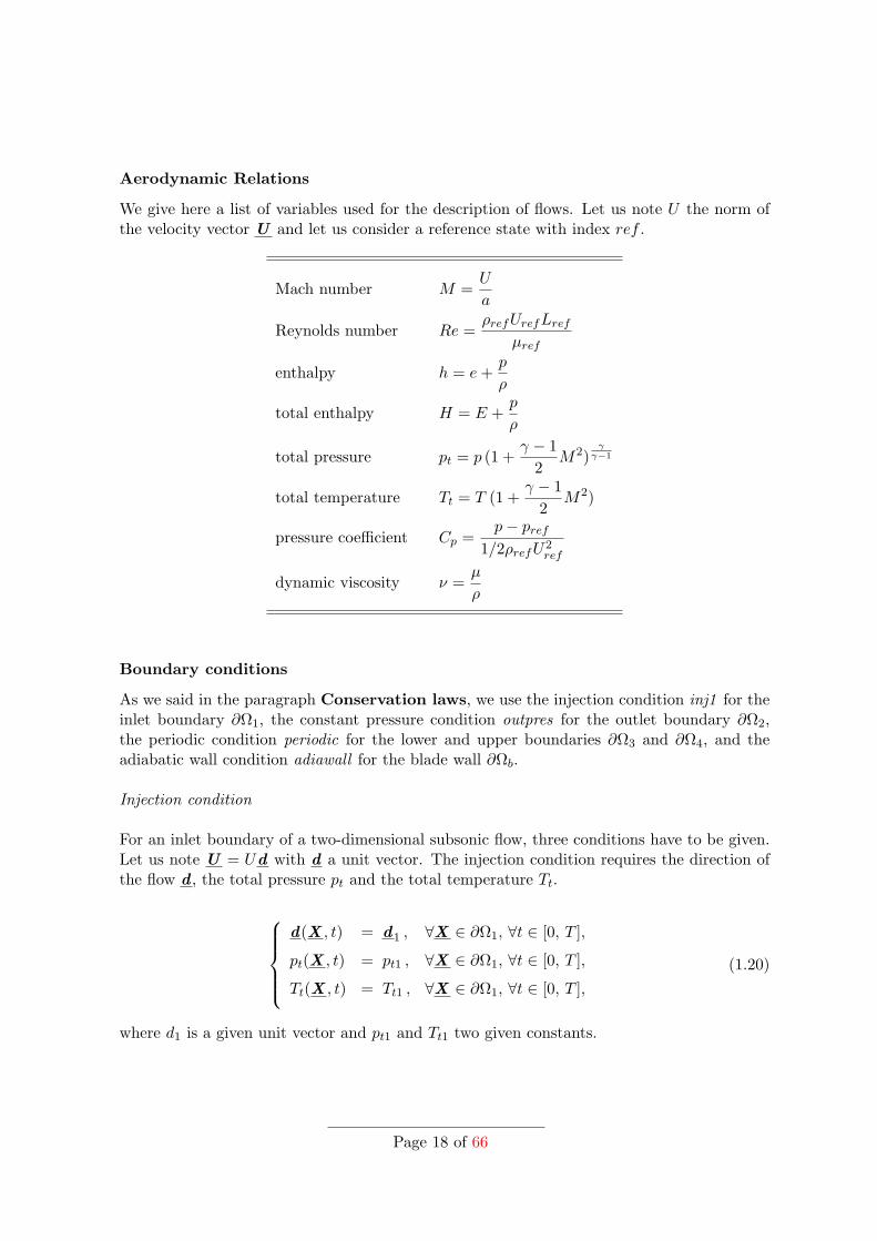
Aerodynamic Relations

We give here a list of variables used for the description of flows. Let us note U the norm ofthe velocity vector U and let us consider a reference state with index ref .

Mach number M =U

a

Reynolds number Re =ρrefUrefLref

µref

enthalpy h = e+p

ρ

total enthalpy H = E +p

ρ

total pressure pt = p (1 +γ − 1

2M2)

γγ−1

total temperature Tt = T (1 +γ − 1

2M2)

pressure coefficient Cp =p− pref

1/2ρrefU2ref

dynamic viscosity ν =µ

ρ

Boundary conditions

As we said in the paragraph Conservation laws, we use the injection condition inj1 for theinlet boundary ∂Ω1, the constant pressure condition outpres for the outlet boundary ∂Ω2,the periodic condition periodic for the lower and upper boundaries ∂Ω3 and ∂Ω4, and theadiabatic wall condition adiawall for the blade wall ∂Ωb.

Injection condition

For an inlet boundary of a two-dimensional subsonic flow, three conditions have to be given.Let us note U = Ud with d a unit vector. The injection condition requires the direction ofthe flow d , the total pressure pt and the total temperature Tt.

d(X , t) = d1 , ∀X ∈ ∂Ω1, ∀t ∈ [0, T ],

pt(X , t) = pt1 , ∀X ∈ ∂Ω1, ∀t ∈ [0, T ],

Tt(X , t) = Tt1 , ∀X ∈ ∂Ω1, ∀t ∈ [0, T ],(1.20)

where d1 is a given unit vector and pt1 and Tt1 two given constants.

of 66

Constant pressure condition

For a subsonic flow, there is only one condition to be imposed on the outlet boundary. Weuse here a constant pressure condition :

p(X , t) = p2 , ∀X ∈ ∂Ω2, ∀t ∈ [0, T ], (1.21)

where p2 is a given constant.

Periodic condition

We use a condition of periodicity between the upper and lower boundaries : the fluxes whichcomes through the lower boundary ∂Ω3 are reinjected through the upper boundary ∂Ω4 andvice versa. The variables [ρ, ρU T, ρE]T and the fluxes are equal on ∂Ω3 and ∂Ω4.

Adiabatic wall condition

The blade wall ∂Ωb is supposed to be adiabatic which means there is not any heat trans-fer between the flow and the blade. This can be written as :

∇ p(X , t) = 0 , ∀X ∈ ∂Ωb, ∀t ∈ [0, T ],

U (X , t) = 0 , ∀X ∈ ∂Ωb, ∀t ∈ [0, T ],

q(X , t) = 0 , ∀X ∈ ∂Ωb, ∀t ∈ [0, T ].

(1.22)

1.4.2 Modeling of the turbulence : RANS equations

The nonlinear part ∇ · (ρU ⊗U ) of the convective flux in the Navier-Stokes equations (1.12)is responsible of the turbulence. When the Reynolds number of the flow is low, the diffusiveflux −∇ · τ is high enough compared to the convective flux to cancel the non-linearities :the flow is laminar. But from a certain Reynolds number (the laminar-turbulent transitionis a whole subject and we do not discuss about this here), the convective flux becomes sohigh that it is the most dominant effect : the flow is turbulent. Turbulent flows appear asan instability of laminar flows. They involve activity over a continuous spectrum of lengthand time scales, are random in appearance, chaotic, irregular with a high sensibility to thedetails of boundary and initial conditions. They are three-dimensional, unsteady and havea rotational and dissipative nature. To calculate all the length scales, the required numberof points of the grid (obtained via discretization of the domain Ω, see subsection 1.3.3) ishuge. For three-dimensional flows, this number N3D is proportional to Re 9/4 where Re isthe Reynolds number. For our applications, Re = 264170 which yields N3D ∼ 1012. Theturbulence is therefore not calculated but modeled via a statistically approach.

Reynolds and Favre averages

A turbulent flow can be described statistically. Reynolds [34] introduced the so-called Reynolds-averaged Navier-Stokes (RANS) equations using a decomposition of a field g(X , t) (scalar or

of 66

vector) in a mean part g(X , t) and a fluctuation part g′(X , t) :

g(X , t) = g(X , t) + g′(X , t),

with g(X , t) = limn→∞

1n

n∑k=1

gk(X , t) and g′ = 0. (1.23)

This is an average over the realizations gk of the field. In our applications, we only considersteady turbulent flows which means that the statistical average g does not depend on thetime. In this case, statistical and time averages can be identified (ergodicity hypothesis, [12])and g can be defined as :

g(X , t) =1T

t0+T

t0

g(X , t) dt, (1.24)

where T is greater than the characteristic period of the fluctuations g′. The Reynolds averageis actually only used for incompressible flows. For compressible flows, the Favre average ispreferred. The Favre average of a field g(X , t) is :

g(X , t) =ρ(X , t)g(X , t)

ρ(X , t), (1.25)

where ρg and ρ are Reynolds averages. The field g can then be decomposed as :

g(X , t) = g(X , t) + g′′(X , t),

with ρg′′ = 0 but g′′ 6= 0.(1.26)

Reynolds-averaged Navier-Stokes equations

Using the Favre average (1.26) for the Navier-Stokes equations (1.12), we get the RANSequations (for the details of the calculation, see [4]) :

∂ρ

∂t+ ∇ · (ρU ) = 0,

∂ρU

∂t+ ∇ · (ρU ⊗U + pI − τ − τt) = 0,

∂ρ(E + k)∂t

+ ∇ · (ρ(E + k)U + pU − (τ + τt)U + q + qt) = 0,

(1.27)

with initial conditions ρ(X , 0) = ρ0(X ), (ρU )(X , 0) = (ρU )0(X ), (ρE)(X , 0) = (ρE)0(X ),for all X in Ω. To simplify the equations (1.27) and the initial conditions, the mean flowvariables don’t have been overlined : ρ and p are Reynolds-averaged, U and E are Favre-averaged. The stress tensor τ and the heat flux vector q have the same expressions asequations (1.17) and (1.19), replacing U and T by U and T . Finally, there are only threenew contributions : the Reynolds stress tensor τt = −ρU ′′ ⊗U ′′, the turbulent kinetic energy

k = 1/2ρU ′′2/ρ and the turbulent heat flux vector qt = cP ρT ′′U′′.

of 66

Boussinesq’s hypothesis

To close the system (1.27), the turbulence has to be modeled through the modeling of τt, kand qt. Boussinesq introduced in 1877 the concept of turbulent viscosity µt. He modeled theeffect of the turbulence on the mean flow as an augmentation of the viscosity and defined theReynolds stress tensor τt and the turbulent heat flux vector qt as :

τt = −23

(ρk + µt∇ ·U )I + µt

[∇U + ∇U T

],

qt = −cPµtPrt

∇T .(1.28)

Prt is the turbulent Prandtl number, constant and equal to 0.9 for our applications.The Boussinesq’s hypothesis simplifies the modeling of the turbulence, reducing the numberof unknowns to two : k and µt.

Turbulence model

It exists a lot of different models to calculate k and µt. These models can be either algebraicalmodels or models using one or two convection equations. Balwin-Lomax [3] and Michel[24] models are algebraical models, the k − ε model of Jones-Launder [20] and the k − ωmodel of Wilcox [45] are 2-equation models. We use in this thesis the 1-equation Spalart-Allmaras model [41]. This model uses a convection equation for the modified turbulentdynamic viscosity νt, proportional to the turbulent dynamic viscosity νt far from the wall.The turbulent kinetic energy k is not modeled : for flows having a moderate level of turbulence,k can be neglected using a well chosen normalization. The effect of the turbulence is thereforeonly modeled through the turbulent viscosity µt.

Initial and boundary conditions

The boundary conditions are the same for the boundaries ∂Ω1, ∂Ω2, ∂Ω3 and ∂Ω4, and ∂Ωb :injection, constant pressure, periodic and adiabatic conditions respectively. Initial conditionsof [ρ, ρU T, ρE]T are also given. There is an initial condition of µt and boundary conditions :fixed values on ∂Ω1 and ∂Ω2, periodic condition between ∂Ω3 and ∂Ω4, and equal to 0 on∂Ωb.

1.4.3 Discretization of the RANS equations with the Finite Volume Method

The elsA software uses the Finite Volume Method (FVM) for the discretization of the RANSequations (1.27). The three-dimensional domain Ω is a multi-block mesh with structuredblocks divided into hexahedral cells Ωi,j,k (a cell of a structured grid is located by threeindexes i, j and k). The six faces are denoted by Σi+1/2,j,k, Σi−1/2,j,k, Σi,j+1/2,k, Σi,j−1/2,k,Σi,j,k+1/2 and Σi,j,k−1/2. The unknowns (ρ, ρU , ρE) are averaged into each cell and stored inthe center of the cell (cell-centred method).

of 66

Spatial discretization

Let us note :

- W = [ρ, ρU T, ρE]T the vector of conservative variables or state vector,

- Fc(W ) =[ρU , (ρU ⊗U ) + pI, ρEU + pU

]Tthe convective flux matrix,

- Fd(W ,∇W ) =[(0

00

),−(τ + τt),−(τ + τt)U + (q + qt)

]Tthe diffusive flux matrix,

and F = Fc + Fd the flux matrix. Let us integrate the RANS equations (1.27) in the cellΩi,j,k with the notations we have just introduced. We get then the integrated form of theRANS equations :

d

dt

Ωi,j,k

W dΩ +

Σi,j,k

[Fc(W ) + Fd(W ,∇W )

]n dΣ = 0, (1.29)

with Σi,j,k = Σi+1/2,j,k ∪Σi−1/2,j,k ∪Σi,j+1/2,k ∪Σi,j−1/2,k ∪Σi,j,k+1/2 ∪Σi,j,k−1/2. To simplify,we forget the indexes (i, j, k) and we get then :

d

dt

ΩW dΩ +

Σ

[Fc(W ) + Fd(W ,∇W )

]n dΣ = 0. (1.30)

Let us note Σ = ∪6p=1Σp and VΩ =

Ω dΩ the volume of the cell Ω. Let us define :

W Ω =1VΩ

ΩW dΩ , (1.31)

the average value of W in the cell Ω and :

F Σp =

Σp

[Fc(W ) + Fd(W ,∇W )

]np dΣ , (1.32)

the flux through the face Σp. (1.30) can be rewritten :

d

dt(VΩ W Ω) = −

6∑p=1

F Σp . (1.33)

For the discretization of (1.33), we have first to choose a numerical approximation W appΩ of

W Ω : W appΩ is simply the value of W in the center of Ω. We have then to choose a numerical

approximation of F Σp . (1.33) is one more time rewritten :

d

dt(VΩ W app

Ω ) = −6∑p=1

F app(W app

Ω ,W appΩ1p, ...,W app

ΩNpp

)n Σp , (1.34)

with n Σp =

Σpnp dΣ and the cells Ωi

p are the Np neighbor cells of Ω used for the calculationof the flux on the interface Σp. For our applications the grid does not depend on the timeand consequently VΩ neither.

of 66

Equation (1.34) becomes finally :

d

dtW app

Ω = − 1VΩ

6∑p=1

F app(W app

Ω ,W appΩ1p, ...,W app

ΩNpp

)n Σp = −R

(W app

Ω

), (1.35)

with R(W app

Ω

)the explicit numerical residual. We have now to choose an approximation

flux matrix F app.

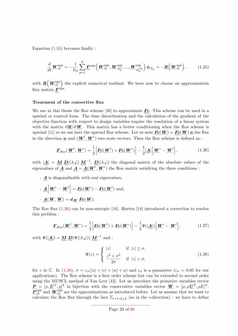
Treatment of the convective flux

We use in this thesis the Roe scheme [36] to approximate Fc. This scheme can be used in aupwind or centred form. The time discretization and the calculation of the gradient of theobjective function with respect to design variables require the resolution of a linear systemwith the matrix ∂R/∂W . This matrix has a better conditioning when the Roe scheme isupwind [11] so we use here the upwind Roe scheme. Let us note Fc(W ) = Fc(W )n the fluxin the direction n and (W l,W r) two state vectors. Then the Roe scheme is defined as :

FRoe(Wl,W r) =

12

[Fc(W l) + Fc(W r)

]− 1

2|A|[W r −W l

], (1.36)

with |A| = M D(|λA|) M−1, D(|λA|) the diagonal matrix of the absolute values of theeigenvalues of A and A = A(W l,W r) the Roe matrix satisfying the three conditions :

- A is diagonalizable with real eigenvalues,

- A[W r −W l

]= Fc(W r)− Fc(W l) and,

- A(W ,W ) = dW Fc(W ).

The Roe flux (1.36) can be non-entropic [18]. Harten [18] introduced a correction to resolvethis problem :

FRoe(Wl,W r) =

12

[Fc(W l) + Fc(W r)

]− 1

2Ψ(|A|)

[W r −W l

], (1.37)

with Ψ(|A|) = M D(Ψ(|λA|)) M−1 and :

Ψ(z) =

|z| if |z| ≥ σ,

z2 + σ2

2σif |z| < σ,

(1.38)

for z in C. In (1.38), σ = εσ(|u| + |v| + |w| + a) and εσ is a parameter (εσ = 0.05 for ourapplications). The Roe scheme is a first order scheme but can be extended to second orderusing the MUSCL method of Van Leer [43]. Let us introduce the primitive variables vectorP = [ρ,U T, p]T in bijection with the conservative variables vector W = [ρ, ρU T, ρE]T.Papp

Ω and W appΩ are the approximations as introduced before. Let us assume that we want to

calculate the Roe flux through the face Σi+1/2,j,k (so in the i-direction) : we have to define

of 66

two states W li+1/2,j,k and W r

i+1/2,j,k in (1.37), or - it is equivalent - two states P li+1/2,j,k and

Pri+1/2,j,k. These two states are defined as :

P li+1/2,j,k = Papp

Ω +12

slopi(i, j, k),

Pri+1/2,j,k = Papp

Ω − 12

slopi(i+ 1, j, k),(1.39)

with slopi the slope in the i-direction defined as :

slopi(i, j, k) = φ(PappΩ −Papp

i−1,j,k,Pappi+1,j,k −Papp

Ω ), (1.40)

and (Pappi−1,j,k,P

appi−1,j,k) the approximations of the vector P in the cells Ωi−1,j,k and Ωi+1,j,k.

φ is a slope’s limiter and we use the one of Van Albada [42] :

φva(a, b) =(b2 + ε)a+ (a2 + ε)b

a2 + b2 + εwith 0 < ε 1. (1.41)

Finally the approximation convective flux through the face Σi+1/2,j,k is :

Fcapp(W app

Ω ,W appΩi−1,j,k

,W appΩi+1,j,k

)n Σi+1/2,j,k

= FRoe

(W l

i+1/2,j,k,Wri+1/2,j,k

). (1.42)

Treatment of the diffusive flux

The diffusive flux matrix Fd involves gradients dependant of the state vector. It involves inparticular the gradient of the temperature ∇T . Let us define a coordinate system (x, y, z)and set ∇T = [∂T/∂x, ∂T/∂y, ∂T/∂z]T. The derivatives are supposed to be uniform in a cellΩ (normal n = [nx, ny, nz]) and we have then via the Green formula for ∂T/∂x :

∂T

∂x=

1VΩ

Ω

∂T

∂xdΩ =

1VΩ

ΣTnx dΣ. (1.43)

The formula (1.43) has then to be discretized and the gradients stored in the center of thecell or in the center of the interfaces. See [28] to know more about the different discretizationschemes available in elsA.

Discretization of the Spalart-Allmaras model

The convection equation is discretized with a first order Roe scheme. Bompard gives theexplicit discretization in his PHD thesis [6].

Time discretization and linearization

Let us recall the equation (1.35) :

d

dtW app

Ω = −R(W app

Ω

).

This equation is then discretized with a first order backward Euler method :

W kΩ −W k−1

Ω

∆tk−1= −R

(W k

Ω

). (1.44)

of 66

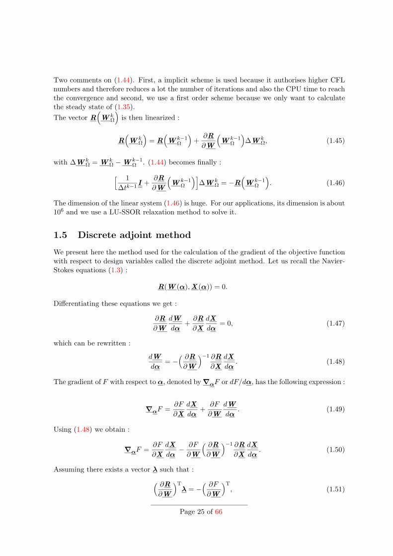
Two comments on (1.44). First, a implicit scheme is used because it authorises higher CFLnumbers and therefore reduces a lot the number of iterations and also the CPU time to reachthe convergence and second, we use a first order scheme because we only want to calculatethe steady state of (1.35).The vector R

(W k

Ω

)is then linearized :

R(W k

Ω

)= R

(W k−1

Ω

)+

∂R

∂W

(W k−1

Ω

)∆W k

Ω, (1.45)

with ∆W kΩ = W k

Ω −W k−1Ω . (1.44) becomes finally :[ 1

∆tk−1I +

∂R

∂W

(W k−1

Ω

)]∆W k

Ω = −R(W k−1

Ω

). (1.46)

The dimension of the linear system (1.46) is huge. For our applications, its dimension is about106 and we use a LU-SSOR relaxation method to solve it.

1.5 Discrete adjoint method

We present here the method used for the calculation of the gradient of the objective functionwith respect to design variables called the discrete adjoint method. Let us recall the Navier-Stokes equations (1.3) :

R(W (α),X (α)) = 0.

Differentiating these equations we get :

∂R

∂W

dW

dα+∂R

∂X

dX

dα= 0, (1.47)

which can be rewritten :

dW

dα= −

( ∂R∂W

)−1 ∂R

∂X

dX

dα. (1.48)

The gradient of F with respect to α, denoted by ∇αF or dF/dα, has the following expression :

∇αF =∂F

∂X

dX

dα+

∂F

∂W

dW

dα. (1.49)

Using (1.48) we obtain :

∇αF =∂F

∂X

dX

dα− ∂F

∂W

( ∂R∂W

)−1 ∂R

∂X

dX

dα. (1.50)

Assuming there exists a vector λ such that :( ∂R∂W

)Tλ = −

( ∂F∂W

)T, (1.51)

of 66

The gradient of F with respect to α can be finally rewritten :

∇αF =∂F

∂X

dX

dα+ λT ∂R

∂X

dX

dα. (1.52)

Let us recall that dX /dα is given by Padge , ∂R/∂X by elsA, ∂F/∂X by Zapp and λthrough the iterative resolution of the equation (1.51). This equation is a linear system ofhuge size nW (∼ 105). The principal interest of this method is that its cost does not dependon the number of design variables and that is why it is used for industrial configurations withhundreds of design variables.Let us say just one word about the resolution of (1.51). We use the so-called frozen-µt [26]approximation. During the mesh deformation, the turbulent viscosity µt does not change :its values are frozen. The principal interest of this approximation is that the expression of∂R/∂W does not depend on the choice and the complexity of the turbulence model.

1.6 Optimization algorithm

We present in this section the optimization algorithm used for the resolution of our problem.Let us recall the single-point optimization problem (1.5) :

Minimize F (W (α),X (α),Π),for Π = Πk given,with respect to α,subject to α ∈ Dα.

(1.53)

All we will say in this section would be the same for F instead of F for multipoint optimizationproblems. The L(imited memory)-BFGS-B(ound constrained) algorithm has been chosen tosolve (1.5). This algorithm, first described by Byrd et al. [8] is a generalization of the L-BFGSalgorithm [27] for optimization problems with bounds. These two algorithms are themselvesan extension of the well known BFGS algorithm, which works for unconstrained optimizationproblems only, described separately in 1970 by Broyden [7], Fletcher [14], Goldfarb [17] andShanno [38].The function F is a non-linear function whose gradient with respect to α is available. Thesethree algorithms don’t require the second derivatives : the Hessian matrix is approximatedusing rank-one updates specified by gradient evaluations. Let us begin with the BFGS algo-rithm for unconstrained optimization problems. To simplify the notations we do not writewith bold font and do not underline vectors and matrices in this section.

of 66

BFGS algorithmChoose an initial guess α0, an initial approximate Hessian matrix H0 and astopping criterion crt (0)Evaluate ∇F (α0) (1)Initialize k ← 0while crt false do

Solve Hkpk = −∇F (αk) to get pk (2)Perform a line search to get an acceptable stepsize ak in the direction pk (3)Update sk ← akpk and αk+1 ← αk + skEvaluate ∇F (αk+1) (4)Update yk ← ∇F (αk+1)−∇F (αk)

Update Hk+1 ← Hk +yky

Tk

yTk sk−Hksks

TkHk

sTkHksk

(5)

Update k ← k + 1end while

The initial approximate Hessian matrix H0 for (0) has to be a symmetric definite positivematrix (usually a diagonal matrix with positive components). The evaluation of the gradientfor (1) and (4) is given trough the resolution of an adjoint equation. The update (5) can bereplaced by an update of the inverse of Hk+1 applying the Shermann-Morrison formula :

H−1k+1 =

(I −

skyTk

yTk sk

)H−1k

(I −

yksTk

yTk sk

)+sks

Tk

yTk sk

. (1.54)

and (2) becomes then simply pk+1 = −H−1k+1∇F (αk+1). See [8] to know more about the line

search (3).The computational cost of one iteration of the algorithm is O(n2

α) since the algorithm requiresonly matrix-vector multiplications. Moreover it is necessary to have nα(nα + 1)/2 storage lo-cations at each iteration since the symmetric matrix Hk (or H−1

k ) has to be kept.

This is precisely the interest of the L-BFGS method which never explicitly forms or storesthis matrix. Instead it stores information from the past m iterations (with m nα) anduses only this information to implicitly do operations requiring the Hessian (or the inverseHessian). Let us set ρk = 1/(yT

k sk) and vk = (I − ρkyksTk ). (1.54) becomes then :

H−1k+1 = vT

kH−1k vk + ρksks

Tk . (1.55)

Instead of storing H−1k in order to update H−1

k+1 (memory cost nα(nα + 1)/2), Nocedal hasshown in [27] that it is equivalent to store (yi, si)0≤i≤k and H−1

0 (memory cost (2(k+1)+1)nαat the kth iteration if H−1

0 is diagonal) and update H−1k+1 with :

of 66

H−1k+1 = vT

k vTk−1 . . . v

T0 H

−10 v0 . . . vk−1vk

+ vTk . . . v

T1 ρ0s0s

T0 v1 . . . vk

...+ vT

k vTk−1ρk−2sk−2s

Tk−2vk−1vk

+ vTk ρk−1sk−1s

Tk−1vk

+ ρksksTk .

(1.56)

The idea of Nocedal is then to choose an integer m (with m nα) and to discard the oldinformation storing only the last m (yi, si). The first m − 1 iterations, L-BFGS and BFGSgenerate the same search direction : for k+ 1 ≤ m (1.56) is used. But for k+ 1 > m a specialupdate is used, which uses only the last m (yi, si) and is given by :

H−1k+1 = vT

k vTk−1 . . . v

Tk−m+1H

−10 vk−m+1 . . . vk−1vk

+ vTk . . . v

Tk−m+2ρk−m+1sk−m+1s

Tk−m+1vk−m+2 . . . vk

...+ vT

k ρk−1sk−1sTk−1vk

+ ρksksTk .

(1.57)

Using (1.56) and (1.57), we only need to have (2m+ 1)nα storage locations at each iteration :if m nα, (2m+1)nα = O(nα) for L-BFGS which has be compared to nα(nα+1)/2 = O(n2

α)for BFGS.

The L-BFGS-B algorithm [8] is not presented here. It uses limited BGGS matrices to ap-proximate the Hessian of the objective function and the gradient projection approach [5] todetermine the active set of constraints.

of 66

Chapter 2

Application for the design of turbomachine blades :minimization of the entropy generation rate around a LS89

blade

Our test case is the LS89 blade of a highly loaded transonic turbine distributor. This bladehas been designed by the Von Karman Institute in the early 1990s and a lot of experimentalstudies have been carried out for very different physical conditions [2].

2.1 Presentation of the two-dimensional test case

We have chosen to focus on the condition MUR235 [2] which corresponds to a nominal con-dition of utilisation. The figure 2.1 shows the mesh used. It is a multi-block mesh withstructured blocks.

Figure 2.1: Mesh of the two-dimensional LS89 test case : 35 blocks, 153 482 cells, 140 330nodes.

The mesh has been cut into many blocks in order to perform parallel computing on 16processors (4 quad-core Intel Xeon Nehalem 2.66 Ghz processors).

of 66

The table 2.1 gives a few geometrical parameters describing the LS89 blade.

chord c (mm) 67.647pitch g/c 0.850leading edge radius rLE/c 0.061trailing edge radius rTE/c 0.0105

Table 2.1: Geometrical parameters of the LS89 blade.

The table 2.2 indicates the Reynolds and Mach numbers on the inlet boundary ∂Ω1.

Re1 264 170M1 0.15

Table 2.2: Reynolds and Mach numbers on the inlet boundary ∂Ω1.

The table 2.3 gives the boundary conditions on the inlet and outlet boundaries ∂Ω1 and ∂Ω2.

Inlet : injection Outlet : constant pressurePt1 (Pa) 182 704.1 Π = Ps2/Ps1 0.583Tt1 (K) 413.3β1 (deg.) 0.0

Table 2.3: Boundary conditions.

The direction of the flow d1 is given by the angle of injection β1.The MUR235 condition corresponds to a transonic flow. There is a shock wave on the uppersurface of the blade and a large turbulent wake from the trailing edge. At this condition theentropy generation rate, calculated via elsA and Zapp (with 16 processors and a CPU cost∼ 3840 seconds), is equal to 9.67%. The stopping criteria for elsA was the number ofiterations (1500) of the CFD calculation chosen in order to get numerical residuals on density∼ 10−6.

2.2 Entropy generation rate minimization without constrainton the mass flow rate and with free leading edge

We study in this section the entropy generation rate minimization without constraint on themass flow rate and with free leading edge.

2.2.1 Setting of the single-point optimization problem

The aim of a turbine is to prepare the flow before arriving in the rotative part, speeding up itand deflecting it. The speed up of the flow is generated by a pressure ratio Π = Ps2/Ps1 < 1on the outlet boundary ∂Ω2. This pressure ratio Π characterizes the flow : a given pressureratio defines a specific condition. The nominal condition MUR235 corresponds to Π = 0.583and from now we note Π = Πnom.In the case of a flow without entropy generation or, and it is equivalent, without loss of total

of 66

pressure, the Mach number on ∂Ω2 is equal to the maximum Mach number which can begenerated by Π, called the isentropic Mach number M2, is. We have in this case the relation :

Ps2Ps1

=(1 +

γ − 12

M21 )

γγ−1

(1 +γ − 1

2M2

2, is)γγ−1

. (2.1)

The relation (2.1) shows that a given pressure ratio Π corresponds to a given M2, is and viceversa : the condition MUR235 corresponds to M2, is = 0.927.The goal is then, from a given ratio Π, to obtain the highest Mach number on ∂Ω2. A way tomaximize M2 is to minimize the entropy generation rate. It is classically used for the shapeoptimization for turbine blades [23, 44]. The entropy generation rate is characterized, fortwo-dimensional distributor turbine flows, by the ratio Pt2/Pt1. More precisely, minimizingthe entropy generation rate is equivalent to maximizing the ratio Pt2/Pt1 so the objectivefunction used is :

F (α) = 1− Pt2(α)Pt1

, (2.2)

and the single-point optimization problem at the condition MUR235 is :

Minimize 1− Pt2(α,Π)Pt1

,

for Π = Πnom,with respect to α,subject to α ∈ Dα.

(2.3)

Let us recall that α is the design variables vector of size nα and that we use a CADparametrization. For our applications nα = 18 (see section 2.2.3). Pt2 is calculated asfollows :

Pt2 =1Q2

X∈∂Ω2

Pt(X ) ρ(X )U (X ) · n2(X ) dΣ, (2.4)

with Q the mass flow rate defined by :

Q =

X∈∂Ω2

ρ(X )U (X ) · n2(X ) dΣ. (2.5)

Equation (2.8) is a mass flow rate average of Pt on ∂Ω2. This kind of average is classicallyused for total variables [35]. Equations (2.8) and (2.9) are calculated by the post-processingtool Zapp.The goal of the optimization is to reduce the shock intensity and the wake width in orderto minimize the entropy generation rate. We present in the section 2.2.4 the results of thesingle-point optimization.

of 66

2.2.2 Setting of the multipoint optimization problem

As we explained in the section 1.1.2, it can be interesting to minimize F not only for thenominal condition Πnom but over a continuous interval of conditions IΠ around Πnom = 0.583.We choose IΠ = [0.506 , 0.633], which corresponds to M2, is = [0.85 , 1.05], and we sample ituniformly with NΠ = 21 > nα = 18. We perform the GSA algorithm and we obtain fivedifferent conditions. The table 2.12 shows these conditions and the corresponding isentropicMach numbers.

of 66

Conditions C01 C05 C15 C17 C21Pressure ratio Π Π01=0.633 Π05=0.607 Π15=0.543 Π17=0.530 Π21=0.506Isentropic Mach number M2, is 0.85 0.89 0.99 1.01 1.05

Table 2.4: Pressure ratios selected by GSA and corresponding isentropic Mach numbers.

The algorithm GSA requires calculations of gradient ∇αF (α,Πk) for the 21 conditions Πk.Each gradient calculation uses all the modules of the optimization process (from Padge toadjoint Padge , see table 1.2 section 1.1.3) and is performed on 16 processors. The CPU costof one iteration of the optimization process is about 7200 seconds.We can now define F :

F (α) = w01 F (α,Π01) + w05 F (α,Π05) + w15 F (α,Π15) + w17 F (α,Π17) + w21 F (α,Π21).

We present in the section 2.2.5 the results of the multipoint optimization with two differenttypes of weights.

2.2.3 Parametrization and gradient validation with finite differences

The LS89 blade has been parametrized with 18 design variables. The trailing edge of theblade has been frozen in order to keep the same direction of the wake (as we said in section2.1.2 the turbine has to prepare the flow before arriving in the rotative part and one of theimportant criteria is the flow deflection). The thicknesses have been also frozen for structuralconstraints.We have compared the values of the gradient ∇αF given by the discrete adjoint method withvalues given by finite differences (using a second order scheme). The number of iterations(800) of the iterative resolution of the adjoint equation (1.51) has been chosen in order toprovide low errors : the average error is equal to 1.86%. The figure 2.2 shows the error withrespect to design variables. We have actually computed ∇α(1000F ) because the derivativeshave a relatively low level and a few modules of the optimization process work only withsingle precision.

0 2 4 6 8 10 12 14 16 180

5

10

15

20

25Error on the gradient with respect to design variables

Design variables ID.

Err

or

(%)

Figure 2.2: Values of the gradient ∇αF given by the discrete adjoint method compared withvalues given by finite differences.

of 66

The design variables #8 and #13 have the highest errors : 19.92% and 5.2%. These twovariables represent curvatures of the blade at two different positions. The result is moreoververy satisfying because the average error is very low.

2.2.4 Results of the single-point optimization

We present in this section the results of the single-point optimization obtained with theLBFGSB algorithm. The figure 2.3 shows the optimization history. The table 2.5 synthesizesthe results.

0 5 10 15 20 25 309.45

9.5

9.55

9.6

9.65

9.7

9.75Evolution of the objective function with design cycles

Design cycles

Ob

ject

ive

fun

ctio

n (

%)

0 5 10 15 20 25 309.75

10.0

10.25

10.50

10.75

No

rmal

ized

mas

s fl

ow

rat

e

Normalized mass flow rateObjective function

Figure 2.3: Evolution of the objective function with design cycles and correlative augmenta-tion of the mass flow rate.

Initial value Final value Variation (%)Entropy generation rate (%) 9.67 9.47 - 2.07Normalized mass flow rate 9.94 10.49 + 5.53

Table 2.5: Inital and final values of the entropy generation rate and the mass flow rate.

A few comments about the figure 2.3. The calculation has been performed on 16 parallelprocessors. The convergence has been reached after 30 iterations of the optimization processand for a CPU cost equal to about 216000 seconds (CPU cost ∼ 7200 seconds per iteration,as said in section 2.1.3). The entropy generation has been successfully reduced of 2.07%.The diminution of total pressure loss has correlatively increased the mass flow rate. In otherwords, a part of the energy which was lost through the shock wave and inside the turbulent

of 66

wake has been given back to the flow, increasing the mass flow rate through ∂Ω2. The figure2.4 compares the initial and final blade geometries.

0 0.1 0.2 0.3 0.4 0.5 0.6 0.7 0.8 0.9 1−1.5

−1.4

−1.3

−1.2

−1.1

−1

−0.9

−0.8

−0.7

−0.6

−0.5

−0.4

−0.3

−0.2

−0.1

0

0.1

0.2

0.3

0.4

0.5Initial and redesigned LS89 blade geometries

x/c

z/c

Initial LS89Redesigned LS89

Figure 2.4: Comparison of initial and final LS89 blade geometries.

The redesigned LS89 blade best guides the flow delaying the flow separation and consequentlythe width of the trailing edge wake. The redesigned geometry is not C2 at the leading edgewhich suggests that the parametrization has to be improved (the leading edge is parametrizedby one radius of curvature and it seems two or more could be a better way to characterize it).Figures 2.5 and 2.6 compare the characteristics of the initial and the redesigned LS89 blades.

0.2 0.25 0.3 0.35 0.4 0.45 0.5 0.55 0.6 0.65 0.7 0.75 0.8 0.85 0.96.5

7

7.5

8

8.5

9

9.5

10

10.5

11Normalized mass flow rate Q vs. pressure ratio Ps2/Ps1

Ps2/Ps1

Q

LS89Redesigned LS89

Figure 2.5: Comparison of the characteristics of the initial and the redesigned LS89 blades.The nominal condition is represented with larger markers.

of 66

0.2 0.25 0.3 0.35 0.4 0.45 0.5 0.55 0.6 0.65 0.7 0.75 0.8 0.85 0.90

5

10

15

20

25

30

35

40

45

50Entropy generation rate 1−Pt2/Pt1 vs. pressure ratio Ps2/Ps1

Ps2/Ps1

1−P

t2/P

t1 (

%)

LS89Redesigned LS89

0.5 0.51 0.52 0.53 0.54 0.55 0.56 0.57 0.58 0.59 0.6 0.61 0.62 0.63 0.646

7

8

9

10

11

12

13


Ps2/Ps1

1−P

t2/P

t1 (

%)

LS89Redesigned LS89


of 66

The figure 2.5 shows that the mass flow rate has been increased all over the characteristic. Fora given geometry, increasing the mass flow rate raises the entropy generation rate. The goalof the optimization is then to design shapes which generate higher mass flow rates withoutincreasing the entropy generation rate : the figure 2.6 indicates the entropy generation ratehas been reduced for a few conditions but also increased for others. The table 2.6 synthesizesthe results on the interval of pressure ratio [0.506 , 0.633].

Condition C21 C17 C15 nominal C05 C01Pressure ratio 0.506 0.530 0.543 0.583 0.607 0.633Variation of entropygeneration rate (%) + 0.76 - 0.15 - 0.90 - 2.07 - 2.21 - 2.51

Table 2.6: Variation of entropy generation rate with respect to pressure ratio.

The objective function has been reduced for conditions C01, C05, C15, C17 and for thenominal condition, but has been increased for condition C21. This is precisely what designerscall a poor design and a way to obtain better designs is given by the multipoint optimization.

2.2.5 Results of the multipoint optimization

We present in this section the results of the multipoint optimization for two types of weights.We present first a multipoint optimization with unit weights and present then a multipointoptimization with non-unit weights. We compute the calculations on 16 parallel processors.The cost of one iteration of the optimization process is here much higher because one iterationof the multipoint optimization corresponds to five iterations of the single-point optimizationprocess since the evaluation of the multipoint objective function requires five single-pointobjective function evaluations.

Unit weights

In this section we use unit weights so the objective function F can be written as follows :

F (α) = F (α,Π01) + F (α,Π05) + F (α,Π15) + F (α,Π17) + F (α,Π21).

The evaluation of each F (α,Πk) is performed on 16 parallel processors so then the optimiza-tion process requires here 16 × 5 = 80 processors. The figure 2.7 shows the optimizationhistory and the table 2.7 synthesizes the results.

Condition C21 C17 C15 nominal C05 C01Pressure ratio 0.506 0.530 0.543 0.583 0.607 0.633Variation of entropygeneration rate (%) - 2.57 - 1.66 - 1.11 - 0.81 - 0.92 - 1.13


of 66

0 5 10 15 20 25 30 35 400.53

0.535

0.54


Design cycles

Ob

ject

ive

fun

ctio

n

7.5

8.0

8.5

9.0

En

tro

py

gen

erat

ion

rat

e (%

)

Entropy generation rate at condition C01Entropy generation rate at condition C05Objective function

0 5 10 15 20 25 30 35 400.53

0.535

0.54


Design cycles

Ob

ject

ive

fun

ctio

n

0 5 10 15 20 25 30 35 4011.0

11.5

12.0

12.5

13.0

13.5

14.0

En

tro

py

gen

erat

ion

rat

e (%

)

Entropy generation rate at condition C15Entropy generation rate at condition C17Entropy generation rate at condition C21Objective function

Figure 2.7: Evolution of the objective function with design cycles and correlative reductionof the entropy generation rate at the five selected conditions.

of 66

The figure 2.7 and the table 2.7 show that the entropy generation rate has been successfullyreduced for all the conditions and even all over the characteristic as shown on the figure2.8. The convergence has been reached after 40 iterations of the optimization process andfor a CPU cost equal to about 1440000 seconds (CPU cost ∼ 7200 × 5 = 36000 seconds periteration, as said in section 2.2.2). The figure 2.9 shows that the given back energy has beentransmitted to the flow through an augmentation of the mass flow rate.

of 66

0.2 0.25 0.3 0.35 0.4 0.45 0.5 0.55 0.6 0.65 0.7 0.75 0.8 0.85 0.90

5

10

15

20

25

30

35

40

45


Ps2/Ps1

1−P

t2/P

t1 (

%)

LS89Redesigned LS89

0.5 0.51 0.52 0.53 0.54 0.55 0.56 0.57 0.58 0.59 0.6 0.61 0.62 0.63 0.646

7

8

9

10

11

12

13


Ps2/Ps1

1−P

t2/P

t1 (

%)

LS89Redesigned LS89


of 66

0.2 0.25 0.3 0.35 0.4 0.45 0.5 0.55 0.6 0.65 0.7 0.75 0.8 0.85 0.96.5

7

7.5

8

8.5

9

9.5

10

10.5


Ps2/Ps1

Q

LS89Redesigned LS89


And finally, the figure 2.10 compares the initial and final LS89 blade geometries.

0 0.1 0.2 0.3 0.4 0.5 0.6 0.7 0.8 0.9 1−1.5

−1.4

−1.3

−1.2

−1.1

−1

−0.9

−0.8

−0.7

−0.6

−0.5

−0.4

−0.3

−0.2

−0.1

0

0.1

0.2

0.3

0.4


x/c

z/c



of 66

The redesigned geometry is one more time not C2 at the leading edge which suggests that theparametrization we used is not very well adapted for this blade.

Non-unit weights

We present in this section results obtained for a multipoint optimization with non-unitweights. The aim is to force the algorithm to target the Pareto front. Let us recall theexpression of F :


If one of the functions, let us say F (α,Π01), can be reduced a lot then the algorithm could justreduce this function and increase the others, just because the descent direction taken to reduceF (α,Π01) is the steepest one. The idea is then to perform a single-point optimization foreach condition (with variation of entropy generation rate ∆egr) and choose the weights equalto the absolute values of 1/∆egr. The table 2.8 gives the variations of entropy generationrate for single-point optimizations and the associated weights.

Condition C21 C17 C15 C05 C01Variations of entropy generation ratefor a single-point optimization ∆egr (%) - 2.24 - 1.53 - 1.47 - 2.08 - 2.63Associated weights 1/∆egr 44.5 65.4 68.0 48.1 38.0

Table 2.8: Variations of entropy generation rate for single-point optimizations and associatedweights for the multipoint optimization.

In practice, the variations ∆egr could be estimated by the designers so the weights are notnecessary calculated with a single-point optimization.We have chosen actually weights equal to 0.1/∆egr in order to obtain reasonable values forthe objective function (let us recall that we compute 1000F (α,Π) and not F (α,Π) for thegradient accuracy). The objective function F is then :

F (α) = 3.08F (α,Π01) + 4.81F (α,Π05) + 6.80F (α,Π15) + 6.54F (α,Π17) + 4.45F (α,Π21).

The evaluation of each F (α,Πk) is performed on 16 parallel processors so then the optimiza-tion process requires here 16 × 5 = 80 processors. The figure 2.11 shows the optimizationhistory and the table 2.9 synthesizes the results.

Condition C21 C17 C15 nominal C05 C01Pressure ratio 0.506 0.530 0.543 0.583 0.607 0.633Variation of entropygeneration rate (%) - 2.35 - 1.58 - 1.06 - 0.71 - 0.77 - 0.90


of 66

0 5 10 15 202.85

2.90

2.95


Design cycles

Ob

ject

ive

fun

ctio

n

7.5

8.0

8.5

9.0

En

tro

py

gen

erat

ion

rat

e (%

)

Entropy generation rate at condition C01Entropy generation rate at condition C05Objective function

0 5 10 15 202.85

2.90

2.95


Design cycles

Ob

ject

ive

fun

ctio

n

11.0

11.5

12.0

12.5

13.0

13.5

14.0

En

tro

py

gen

erat

ion

rat

e (%

)

Entropy generation rate at condition C15Entropy generation rate at condition C17Entropy generation rate at condition C21Objective function

Figure 2.11: Evolution of the objective function with design cycles and correlative reductionof the entropy generation rate at the five selected conditions.

of 66

The figure 2.11 and the table 2.9 shows that the entropy generation rate has been one moretime successfully reduced for all the conditions and even all over the characteristic as shownon the figure 2.12. The convergence has been reached after 10 iterations of the optimizationprocess and for a CPU cost equal to about 360000 seconds The figure 2.13 shows that thisreduction is correlated to an augmentation of mass flow rate.

of 66

0.2 0.25 0.3 0.35 0.4 0.45 0.5 0.55 0.6 0.65 0.7 0.75 0.8 0.85 0.90

5

10

15

20

25

30

35

40

45


Ps2/Ps1

1−P

t2/P

t1 (

%)

LS89Redesigned LS89

0.5 0.51 0.52 0.53 0.54 0.55 0.56 0.57 0.58 0.59 0.6 0.61 0.62 0.63 0.646

7

8

9

10

11

12

13


Ps2/Ps1

1−P

t2/P

t1 (

%)

LS89Redesigned LS89


of 66

0.2 0.25 0.3 0.35 0.4 0.45 0.5 0.55 0.6 0.65 0.7 0.75 0.8 0.85 0.96.5

7

7.5

8

8.5

9

9.5

10

10.5


Ps2/Ps1

Q

LS89Redesigned LS89


The figure 2.14 compares the initial and final LS89 blade geometries.

0 0.1 0.2 0.3 0.4 0.5 0.6 0.7 0.8 0.9 1−1.5

−1.4

−1.3

−1.2

−1.1

−1

−0.9

−0.8

−0.7

−0.6

−0.5

−0.4

−0.3

−0.2

−0.1

0

0.1

0.2

0.3

0.4


x/c

z/c



of 66

2.2.6 Comparison of the two multipoint optimizations

The two multipoint optimizations provide satisfying results (table 2.10).

Condition C21 C17 C15 nominal C05 C01Pressure ratio 0.506 0.530 0.543 0.583 0.607 0.633Variation of entropy generation rate (%) withunit weights - 2.57 - 1.66 - 1.11 - 0.81 - 0.92 - 1.13non-unit weights - 2.35 - 1.58 - 1.06 - 0.71 - 0.77 - 0.90

Table 2.10: Comparison of variations of entropy generation rate for the two multipointoptimizations.

The multipoint optimization with unit weights gives lightly better results but for a CPU costmuch higher (table 2.11).

Unit weights Non-unit weightsNumber of iterations of the optimization process 40 10CPU cost (seconds) 1440000 360000

Table 2.11: Comparison of CPU cost to reach the convergence.

The figure 2.15 compares the two geometries.

0 0.1 0.2 0.3 0.4 0.5 0.6 0.7 0.8 0.9 1−1.5

−1.4

−1.3

−1.2

−1.1

−1

−0.9

−0.8

−0.7

−0.6

−0.5

−0.4

−0.3

−0.2

−0.1

0

0.1

0.2

0.3

0.4

0.5Comparison of the two multipoint redesigned LS89 blade geometries

x/c

z/c

Redesigned LS89 with unit weightsRedesigned LS89 with non−unit weights


of 66

2.3 Entropy generation rate minimization with constraint onthe mass flow rate and with frozen leading edge

The redesigned LS89 of last section is not C2. We have worked then on a new parametriza-tion with 25 design variables and a frozen leading edge. We have performed a single-pointoptimization with it and the results are very different : the entropy generation decreased of0.8% but the mass flow rate also decreased of 2.28%. To avoid the entropy decrease causedby mass flow rate reduction we choose then to minimize the entropy generation rate withconstraint on the mass flow rate and with frozen leading edge.

2.3.1 Setting of the single-point optimization problem

The objective function is then :

F (α,Π) =S(α,Π)S0(Π)

+ σ(Q(α,Π)Q0(Π)

− 1)2, (2.6)

where S(α,Π) is the outlet surface averaged entropy generation rate :

S(α,Π) = 1− Pt2(α,Π)Pt1

, (2.7)

with :

Pt2(α,Π) =1S2

X∈∂Ω2

Pt(X ) dΣ, (2.8)

and Q(α,Π) the mass flow rate :

Q =

X∈∂Ω2

ρ(X )U (X ) · n2(X ) dΣ. (2.9)

The index 0 corresponds of values for the initial LS89 blade. We present in the section 2.3.4the results of the single-point optimization.

2.3.2 Setting of the multipoint optimization problem

As we explained in the section 1.1.2, it can be interesting to minimize F not only for thenominal condition Πnom but over a continuous interval of conditions IΠ around Πnom = 0.583.We choose here a larger set IΠ = [0.476 , 0.732], which corresponds toM2, is = [0.7 , 1.1], and wesample it uniformly. We perform the GSA algorithm and we obtain five different conditions.The table 2.12 shows these conditions and the corresponding isentropic Mach numbers.

of 66

Conditions C01 C05 C14 C17 C21Pressure ratio Π Π01=0.732 Π05=0.680 Π15=0.562 Π17=0.524 Π21=0.476Isentropic Mach number M2, is 0.7 0.78 0.96 1.02 1.1

Table 2.12: Pressure ratios selected by GSA and corresponding isentropic Mach numbers.

The algorithm GSA requires calculations of gradient ∇αF (α,Πk) for the 21 conditions Πk.Each gradient calculation uses all the modules of the optimization process (from Padge toadjoint Padge , see table 1.2 section 1.1.3) and is performed on 16 processors. The CPU costof one iteration of the optimization process is about 7200 seconds.We can now define F :


We present in the section 2.3.5 the results of the multipoint optimization with two differenttypes of weights.

2.3.3 Parametrization and gradient validation with finite differences

The LS89 blade has been parametrized with 25 design variables. The trailing edge of theblade has been frozen in order to keep the same direction of the wake (as we said in section2.2.1 the turbine has to prepare the flow before arriving in the rotative part and one of theimportant criteria is the flow deflection). The thicknesses have been also frozen for structuralconstraints. The leading edge has been frozen to provide C2 geometries.We have compared the values of the gradient ∇αF given by the discrete adjoint method withvalues given by finite differences (using a second order scheme). The number of iterations(800) of the iterative resolution of the adjoint equation (1.51) has been chosen in order toprovide low errors : the average error is equal to 1.65%. The figure 2.2 shows the error withrespect to design variables. We have actually computed ∇α(100F ) because the derivativeshave a relatively low level and a few modules of the optimization process work only withsingle precision.

0 5 10 15 20 250

5

10

15Error on the gradient with respect to design variables

Design variables ID.

Err

or

(%)

Figure 2.16: Values of the gradient ∇αF given by the discrete adjoint method compared withvalues given by finite differences.

of 66

The design variables #1, #9 and #15 have the highest errors : 14.19%, 9.72% and 12.41%.These three variables represent curvatures of the blade at three different positions. The resultis moreover very satisfying because the average error is very low.

2.3.4 Results of the single-point optimization

We present in this section the results of the single-point optimization obtained with theLBFGSB algorithm. The figure 2.17 shows the optimization history. The table 2.13 synthe-sizes the results.

0 5 10 15 209.60

9.65

9.70Evolution of entropy generation rate and mass flow rate with design cycles

Design cycles

En

tro

py

gen

erat

ion

rat

e (%

)

0 2 4 6 8 10 12 14 16 18 209.85

9.90

9.95

No

rmal

ized

mas

s fl

ow

rat

e

Normalized mass flow rateObjective function

Figure 2.17: Evolution of the entropy generation rate with design cycles and correlativeevolution of the constrained mass flow rate.

Initial value Final value Variation (%)Entropy generation rate (%) 9.674 9.613 - 0.627Normalized mass flow rate 9.943 9.939 - 0.043

Table 2.13: Inital and final values of the entropy generation rate and the mass flow rate.

A few comments about the figure 2.17. The calculation has been performed on 16 parallelprocessors. The convergence has been reached after 20 iterations of the optimization processand for a CPU cost equal to about 144000 seconds (CPU cost ∼ 7200 seconds per iteration, assaid in section 2.3.2). The entropy generation has been successfully reduced of 0.627%. Themass flow rate fluctuation is very low and more than acceptable : Wang and his collaborators

of 66

[44] estimate that the maximum acceptable fluctuation is ± 0.5%. The figure 2.18 comparesthe initial and final blades geometries.

0 0.1 0.2 0.3 0.4 0.5 0.6 0.7 0.8 0.9 1−1.5−1.4−1.3−1.2−1.1

−1−0.9−0.8−0.7−0.6−0.5−0.4−0.3−0.2−0.1

00.10.20.30.40.5

Initial and redesigned LS89 blade geometries

x/c

z/c



Figure 2.19 shows the variation of entropy generation rate ∆egr with respect to Ps2/Ps1.

0.45 0.47 0.49 0.51 0.53 0.55 0.57 0.59 0.61 0.63 0.65 0.67 0.69 0.71 0.73 0.75−1.5

−1

−0.5

0

0.5

1

1.5

2

2.5

3Variation of entropy generation rate ∆egr vs. pressure ratio Ps2/Ps1

Ps2/Ps1

∆egr

(%

)

Figure 2.19: Variation of entropy generation rate ∆egr with respect to the pressure ratioPs2/Ps1. The nominal condition is represented with larger markers.

of 66

Figure 2.20 compares the mass flow rate of the initial and the redesigned LS89 blades for thepressure ratios selected by the GSA algorithm.

0.45 0.47 0.49 0.51 0.53 0.55 0.57 0.59 0.61 0.63 0.65 0.67 0.69 0.71 0.73 0.759

9.5

10

10.5Normalized mass flow rate Q vs. pressure ratio Ps2/Ps1

Ps2/Ps1

Q

LS89Redesigned LS89

Figure 2.20: Comparison of the mass flow rate of the initial and the redesigned LS89 bladeswith respect to the pressure ratio Ps2/Ps1. The nominal condition is represented with largermarkers.

The table 2.14 synthesizes the results on the interval of pressure ratio [0.476 , 0.732].

Condition C21 C17 C14 nominal C05 C01Pressure ratio 0.476 0.524 0.562 0.583 0.680 0.732∆egr (%) + 2.414 + 1.326 - 0.354 - 0.627 - 0.899 - 1.012∆Q (%) + 1.238 + 0.617 + 0.052 - 0.043 - 0.493 - 0.708

Table 2.14: Variation of entropy generation rate and mass flow rate with respect to pressureratio.

The entropy generation rate has been reduced for conditions C01, C05, nominal and C14but increased for conditions C17 and C21. Moreover the mass flow rate fluctuation is notacceptable for conditions C01, C17 and C21. This is precisely what designers call a poordesign and a way to obtain better designs is given by the multipoint optimization.

2.3.5 Results of the multipoint optimization

We present in this section the results of the multipoint optimization for two types of weights.We present first a multipoint optimization with unit weights and present then a multipointoptimization with non-unit weights. We compute the calculations on 16 parallel processors.The cost of one iteration of the optimization process is here much higher because one iterationof the multipoint optimization corresponds to five iterations of the single-point optimization

of 66

process since the evaluation of the multipoint objective function requires five single-pointobjective function evaluations.

Unit weights

In this section we use unit weights so the objective function F can be written as follows :

F (α) = F (α,Π01) + F (α,Π05) + F (α,Π14) + F (α,Π17) + F (α,Π21).

The figure 2.21 shows the optimization history and compares the initial and final LS89 bladegeometries.

of 66

0 5 10 15 20 25 30 354.975

5.000

5.025

5.050


Design cycles

Ob

ject

ive

fun

ctio

n

0 0.1 0.2 0.3 0.4 0.5 0.6 0.7 0.8 0.9 1−1.5

−1.4

−1.3

−1.2

−1.1

−1

−0.9

−0.8

−0.7

−0.6

−0.5

−0.4

−0.3

−0.2

−0.1

0

0.1

0.2

0.3

0.4


x/c

z/c


Figure 2.21: Evolution of the objective function with design cycles and comparison of initialand final LS89 blade geometries.


of 66

0.45 0.47 0.49 0.51 0.53 0.55 0.57 0.59 0.61 0.63 0.65 0.67 0.69 0.71 0.73 0.75−1.5

−1

−0.5

0

0.5

1

1.5

2

2.5


Ps2/Ps1

∆egr

(%

)



0.45 0.47 0.49 0.51 0.53 0.55 0.57 0.59 0.61 0.63 0.65 0.67 0.69 0.71 0.73 0.759

9.2

9.4

9.6

9.8

10


Ps2/Ps1

Q

LS89Redesigned LS89



of 66

Condition C21 C17 C14 nominal C05 C01Pressure ratio 0.476 0.524 0.562 0.583 0.680 0.732∆egr (%) - 0.917 - 1.053 + 0.040 + 0.148 - 0.039 - 0.083∆Q (%) + 0.021 + 0.054 + 0.012 - 0.030 - 0.131 - 0.176


The entropy generation rate has been reduced for conditions C01, C05, C17, and C21 butincreased for the nominal condition and condition C14. The mass flow rate fluctuations areacceptable. This is not a good optimization since the entropy generation increased for a fewconditions and in particularly for the nominal one. Using non-unit weights seems then theonly way to get better results.

of 66

Non-unit weights

In this section we use non-unit weights equal to 1/∆egr. The figure 2.24 shows the optimiza-tion history and compares the initial and final LS89 blade geometries.

0 5 10 15 20590.5

591

591.5

592

592.5

593Evolution of the objective function with design cycles

Design cycles

Ob

ject

ive

fun

ctio

n

0 0.1 0.2 0.3 0.4 0.5 0.6 0.7 0.8 0.9 1−1.5

−1.4

−1.3

−1.2

−1.1

−1

−0.9

−0.8

−0.7

−0.6

−0.5

−0.4

−0.3

−0.2

−0.1

0

0.1

0.2

0.3

0.4


x/c

z/c


Figure 2.24: Evolution of the objective function and comparison of geometries.

of 66


0.45 0.47 0.49 0.51 0.53 0.55 0.57 0.59 0.61 0.63 0.65 0.67 0.69 0.71 0.73 0.75−1

−0.9

−0.8

−0.7

−0.6

−0.5

−0.4

−0.3

−0.2

−0.1


Ps2/Ps1

∆egr

(%

)



0.45 0.47 0.49 0.51 0.53 0.55 0.57 0.59 0.61 0.63 0.65 0.67 0.69 0.71 0.73 0.759

9.2

9.4

9.6

9.8

10


Ps2/Ps1

Q

LS89Redesigned LS89


of 66


Condition C21 C17 C14 nominal C05 C01Pressure ratio 0.476 0.524 0.562 0.583 0.680 0.732∆egr (%) - 0.420 - 0.904 - 0.168 - 0.075 - 0.227 - 0.264∆Q (%) + 0.175 + 0.040 - 0.026 - 0.072 - 0.210 - 0.273


The entropy generation rate has been successfully reduced for all conditions. The mass flowrate fluctuations are acceptable. This is a good optimization.

of 66

Acknowledgements

Airbus and EADS Innovation Works companies are gratefully acknowledged for makingavailable the optimization chain and its associated tools.

of 66

Conclusion

In the present master thesis a numerical aerodynamic design technique for 2D turbineblades, based on a multipoint shape optimization with discrete adjoint method, has beendeveloped and validated in an environment involving industrial numerical codes.

I worked first on a bibliography of both applied mathematics (optimization, Finite VolumeMethod, parametrization with non-uniform B-splines) and aerodynamics (turbine character-istics, turbulence models). I focused then on the choice of the test case flow characteristics(boundary conditions, Reynolds and Mach numbers, turbulence model) and on the sensitivityof the flow variables with respect to these characteristics. I have also analysed the sensitivityof the flow variables with respect to the numerical parameters of the CFD solver (number ofiterations, CFL number) and to the turbulence model. Once the flow calculation was cor-rectly set I have worked on the parametrization of the blade. A few different parametrizationshave been tested from 18 to 53 variables, with and without frozen variables. One of the mostimportant part of this work was the setting of the optimization problem. A few objectivefunctions have been tested (aerodynamic drag, surface averaged pressure ratio, mass flow rateaveraged pressure ratio) and with or without constraints formulations have been tried. Thegradient of the objective function with respect to the design variables has been validated withfinite differences and the choice of the optimization algorithm has been then driven by thesetting of the optimization problem.

The single-point optimization has engendered a poor design, decreasing the objective func-tion at the targeted condition but increasing it for some others around. The results of themultipoint optimization have been on the other hand very satisfying. The redesigned bladeshave lower entropy generation rate for all the conditions.

This method has now to be adapted to more complex configurations (e.g. 3D rotor turbineconfigurations). The discrete adjoint method does not have been validated at CERFACS forsuch rotative configurations. The entropy generation rate could be replace by the isentropicratio. It would be also interesting to optimize with a larger set of conditions IΠ. An otherpossible work would be to perform the GSA algorithm at each iteration of the optimizationprocess in order to see if the dimension of the Kα, NΠ

spaces varies during the optimizationprocess.

of 66

Bibliography

[1] C.S. Ahn and K.Y. Kim. Aerodynamic design optimization of a compressor rotor withNavier-Stokes analysis. In Proceedings of the Institution of Mechanical Engineers, volume217, pages 179–183, 2003.

[2] T. Arts, M. Lambert De Rouvroit, and A. W. Rutherford. Aero-thermal investigationof a highly loaded transonic turbine guide vane cascade. Technical Report 174, VonKarman Institute, 1990.

[3] B.S. Baldwin and H. Lomax. Thin layer approximation and algebraic model for separatedturbulent flows. AIAA Paper, 1978-257, 1978.

[4] A. Barthet. Amelioration de la prevision des coefficients aerodynamiques autour deconfigurations portantes par la methode adjointe. PhD thesis, Institut National Poly-technique de Toulouse, 2007.

[5] D.P. Bertsekas. Projected Newton methods for optimization problems with simple con-straints. SIAM Journal of Control and Optimization, 20:221–246, 1982.

[6] M. Bompard. Modeles de substitution pour l’optimisation globale de forme enaerodynamique et methode locale sans parametrisation. PhD thesis, Universite de Nice-Sophia Antipolis, 2011.

[7] C. G. Broyden. The convergence of a class of double-rank minimization algorithms.Journal of the Institute of Mathematics and Its Applications, 6:76–90, 1970.

[8] R.H. Byrd, P. Lu, J. Nocedal, and C. Zhu. A limited memory algorithm for boundconstrained optimization. Technical Report NAM-08, Northwestern University, 1994.

[9] L. Cambier and M. Gazaix. elsA : An efficient object-oriented solution to CFD complex-ity. AIAA Paper, 2002-0108, 2002.

[10] L. Cambier, M. Gazaix, S. Heib, S. Plot, P. Poinot, J.P. Veuillot, J.F. Boussuge, andM. Montagnac. CFD Platforms and Coupling : An Overview of the Multi-Purpose elsAFlow Solver. Aerospace Lab, Issue 2, March 2011.

[11] M. Cormery. De l’optimisation aerodynamique vers l’optimisation multidisciplinaire dansun contexte industriel. PhD thesis, Universite Paul Sabatier de Toulouse, 2000.

[12] J. Cousteix. Turbulence et couche limite. Cepadues, 1989.

of 66

[13] J.A. Desideri and A. Janka. Multilevel Shape Optimization for Aerodynamic Opti-mization. In European Congress on Computational Methods in Applied Sciences andEngineering in Jyvaskyla (Finland), 2004.

[14] R. Fletcher. A new approach to variable metric algorithms. Computer Journal, 13:317–322, 1970.

[15] F. Gallard, M. Meaux, M. Montagnac, and B. Mohammadi. Aerodynamic aircraft designfor mission performance by multipoint optimization. In 21st AIAA Computational FluidDynamics Conference, pages –. American Institute of Aeronautics and Astronautics, June2013. Design Optimization Techniques I.

[16] F. Gallard, M. Montagnac, B. Mohammadi, and M. Meaux. Robust parametric shapedesign by multipoint optimization. Technical Report TR-CFD-12-33, CERFACS, 2012.

[17] D. Goldfarb. A family of variable metric updates derived by variational means.Mathematics of Computation, 24:23–26, 1970.

[18] A. Harten and J.M. Hyman. Self-adjusting grid methods for one-dimensional hyperbolicconservation laws. Journal of Computational Physics, 50:235–269, 1983.

[19] A. Jameson. Aerodynamic Design via Control Theory. Journal of Scientifing Computing,3(3):233–260, 1988.

[20] W.P. Jones and Launder B.E. The prediction of laminarization with a two-equationmodel of turbulence. International Journal of Heat and Mass Transfer, 15:301–314,1972.

[21] Gaetan K. W. Kenway and Joaquim R. R. A. Martins. Multi-point High-fidelityAerostructural Optimization of a Transport Aircraft configuration. Journal of Aircraft,2013.

[22] J. Laurenceau. Surface de Reponse par Krigeage pour l’Optimisation de formesAerodynamiques. PhD thesis, INP Toulouse, 2008.

[23] W. Li, L. Huyse, and Padula S. Robust airfoil optimization to achieve consistent dragreduction over a Mach range. Structural and Multidisciplinary Optimization, 24(1):28–50, 2002.

[24] M. Michel, C. Quemard, and R. Durant. Application d’un schema de longueur de melangea l’etude des couches limites turbulentes d’equilibre. Technical Report 154, ONERA,1969.

[25] S.K. Nadarajah and A. Jameson. A comparaison of the continuous and discrete adjointapproach in automatic aerodynamic optimization. AIAA Paper, 00-0667, 2000.

[26] E.J. Nielsen and W.K. Anderson. Aerodynamic design optimization on unstructuredmeshes using the Navier-Stokes equations. AIAA Journal, 37:1411–1419, 1999.

[27] J. Nocedal. Updating quasi-newton matrices with limited storage. Mathematics ofComputation, 35(151):773–782, 1980.

of 66

[28] C. Pham. Linearisation du flux visqueux des equations de Navier-Stokes et de modelesde turbulence pour l’optimisation aerodynamique en turbomachines. PhD thesis, EcoleNationale Superieure d’Arts et Metiers, 2006.

[29] S. Pierret and R.A. Van den Braembussche. Turbomachinery blade design using a Navier-Stokes solver and artificial neural network. Journal of Turbomachinery, 121:326–332,1999.

[30] O. Pironneau. On optimum profiles in Stokes flows. Journal of Fluid Mechanics,59(01):117–128, 1973.

[31] G. Puigt, M. Gazaix, M. Montagnac, M.C. Le Pape, M. De la Llave Plata, C. Marmignon,J.F. Boussuge, and C. Couaillier. Development of a new hybrid compressible solver insidethe CFD elsA software. In Proceedings of the 20th AIAA Computational Fluid DynamicsConference, 2011.

[32] D. Quagliarella and A.D. Cioppa. Genetic algorithms applied to the aerodynamic designof transonic airfoils. Journal of Aircraft, 32(4):889–891, 1995.

[33] J. Reuther, A. Jameson, J. Farmer, L. Martinelli, and D. Saunders. Aerodynamic shapeoptimization of complex aircraft configurations via an adjoint formulation. In Proceedingsof the 34th AIAA Aerospace Sciences Meeting and Exhibit in Reno (USA), 1996.

[34] O. Reynolds. An experimental investigation of the circumstances which determinewhether the motion of water shall be direct and sinous, and of the law of resistancein parallel channels. Proceedings of the Royal Society of London, 35:84–99, 1883.

[35] N. Rochuon. Analyse de l’ecoulement tridimensionnel et instationnaire dans uncompresseur centrifuge avec fort taux de pression. PhD thesis, Ecole centrale de Lyon,2007.

[36] P.L. Roe. Approximate Riemann solvers, parameter vectors and difference schemes.Journal of Computational Physics, 43:357–372, 1981.

[37] J.A. Samareh. Novel Multidisciplinary Shape Parametrization Approach. Journal ofAircraft, 38:1015–1024, 2001.

[38] D.F. Shanno. Conditioning of quasi-newton methods for function minimization.Mathematics of Computation, 24:647–656, 1970.

[39] H. Sobieczky. Parametric Airfoils and Wings. Notes on Numerical Fluid Mechanics,68:71–88, 1998.

[40] T.W. Soderberg and S.R. Perry. Free-form Deformation of polygonal data. In Proceedingsof the International Electronic Image Week in Nice (France), pages 633–639, 1986.

[41] P.R. Spalart and S.R. Allmaras. A one-equation turbulence model for aerodynamic flows.AIAA Paper, 1992-0439, 1992.

[42] G.D. Van Albada, B. Van Leer, and W.W. Roberts. A comparative study of computa-tional methods in cosmic gas dynamics. Astronomy and Astrophysics, 108:76–84, 1982.

of 66

[43] B. Van Leer. Towards the ultimate conservative difference schemes. Journal ofComputational Physics, 32:101–136, 1979.

[44] D.X. Wang and L. He. Adjoint aerodynamic design optimization for blades in multistageTurbomachinery. Journal of Turbomachinery, 132, 2010.

[45] D.C. Wilcox. A two-equation turbulence model for wall-bounded and free-shear flows.AIAA Paper, 1993-2905, 1993.

[46] H. Wu, F. Liu, and H. Tsai. Aerodynamic design of turbine blades using an adjointequation method. AIAA Paper, 05-1006, 2005.

of 66

multipoint shape optimization with discrete adjoint method ...cfdbib/repository/wn_cfd_13_74.pdf ·...

Documents