multitemporal satellite images for urban change detection437205/fulltext01.pdf · the pythagorean...

AG132X Degree Project in Built Environment, First Level Kungliga Tekniska Högskolan Royal Institute of Technology Spring 2011

Multitemporal Satellite Images for Urban Change

Detection

Author: Linda Fröjse Supervisor: Professor Yifang Ban

Geodesy and Geoinformatics, KTH

2

Preface This thesis is the last project for obtaining a Bachelor’s degree in Geomatic Engineering at the Royal Institute of Technology, Stockholm, Sweden.

I would like to thank my supervisor Prof. Yifang Ban for guiding me through the process of change detection, giving critical input on the result and helping me finalizing the thesis. A thank you goes to Osama Yousif for helping me with one algorithm that unfortunately did not work out with my images. I would also like to thank Jan Haas for technical support and encouragement during all of the stages.

Finally I would like to thank my boyfriend for providing me with support and food during the entire process, even though you were busy with your Master thesis in Biotechnology.

3

Abstract The objective of this research is to detect change in urban areas using two satellite images (from 2001 and 2010) covering the city of Shanghai, China. These satellite images were acquired by Landsat-7 and HJ-1B, two satellites with different sensors. Two change detection algorithms were tested: image differencing and post-classification comparison. For image differencing the difference image was classified using unsupervised k-means classification, the classes were then aggregated into change and no change by visual inspection. For post-classification comparison the images were classified using supervised maximum likelihood classification and then the difference image of the two classifications were classified into change and no change also by visual inspection. Image differencing produced result with poor overall accuracy (band 2: 24.07%, band 3: 25.96%, band 4: 46.93%), while post-classification comparison produced result with better overall accuracy (90.96%). Post-classification comparison works well with images from different sensors, but it relies heavily on the accuracy of the classification. The major downside of the methodology of both algorithms was the large amount of visual inspection.

Sammanfattning Detta kandidatarbete behandlar digital förändringsanalys av två satellitbilder (en från 2001 och en från 2010) på Shanghai, Kina från två olika satelliter med två olika sensorer. Två metoder testades på materialet: bildalgebra (subtraktion) och postklassificeringsjämförelse.

Subtraktionsbilden från den bildalgebraiska förändringsanalysen klassificerades med oövervakad klassifikation (k-means) och klasserna aggregerades sen till förändring och icke-förändring med hjälp av visuell jämförelse.

För postklassificeringsjämförelsen klassificerades bilderna var för sig med maximum likelihood klassifikation och subtraktionsbilden av klassifikationerna klassificerades till förändring och icke-förändring, även här med visuell jämförelse.

Bildalgebra gav ett resultat med låg tillförlitlighet, medan postklassificeringsjämförelse gav ett resultat med högre tillförlitlighet. Postklassificeringsjämförelse fungerar bra med bilder från olika sensorer, men kvalitén på analysen beror mycket på klassifikationens tillförlitlighet. Den största nackdelen med metodologin i båda algoritmerna var den stora mängden av visuell jämförelse.

4

Table of ContentsPreface ............................................................................................................................ 2

Abstract .......................................................................................................................... 3

Sammanfattning ............................................................................................................ 3

1. Introduction ............................................................................................................... 6

2. The Process of Change Detection .............................................................................. 7

2.1 Preprocessing ....................................................................................................... 7

2.1.1 Geometric Correction ..................................................................................... 7

2.1.2 Radiometric Correction ................................................................................. 9

2.1 .3 Classifications ............................................................................................. 10

2.2 Change Detection Algorithms ............................................................................ 11

2.2.1 Image Differencing ...................................................................................... 11

2.2.2 Change Vector Analysis .............................................................................. 12

2.2.3 Image Ratioing ............................................................................................. 14

2.2.4 Post-Classification Comparison .................................................................. 15

2.3 Accuracy Assessments ....................................................................................... 16

2.3.1 Classifications .............................................................................................. 16

2.3.2 Change Detection ......................................................................................... 16

3. Study Area and Data Description ........................................................................... 18

4. Methodology ............................................................................................................. 20

4.1 Geometric and Radiometric Correction ............................................................. 21

4.2 Image Differencing ............................................................................................. 21

4.3 Post-Classification Comparison ......................................................................... 22

4.4 Accuracy Assessment ......................................................................................... 22

5. Results and Discussion ............................................................................................ 22

5.1. Change Detection using Image Differencing ................................................... 23

5.2 Change Detection using Post-Classification Comparison ................................ 26

5.2 Accuracy Assessment ......................................................................................... 27

5.2.1 Classifications .............................................................................................. 27

5.2.2 Change Detection ......................................................................................... 27

5

6. Conclusions .............................................................................................................. 30

7. References ................................................................................................................ 31

8. Appendices ............................................................................................................... 34

Appendix A – The Result ......................................................................................... 34

Appendix 1 – Result of K-means Classification – Band 3 ...................................... 40



Appendix 4 – Accuracy of HJ-1B 2010 image classification ................................... 43

Appendix 5 – Separability Matrix for Classification of HJ-1B 2010 image........... 45

Appendix 6 – Accuracy of Landsat-7 ETM+ 2001 image Classification ................ 46

Appendix 7 – Separability Matrix of Landsat-7 ETM+ 2001 Image Classification................................................................................................................................... 49

Appendix 8 – Accuracy Assessment Report for Post-Classification Comparison .. 50

Appendix 9 – Accuracy Assessment Report for Image Differencing with Band 3 . 52

Appendix 10 – Accuracy Assessment Report for Image Differencing with Band 2................................................................................................................................... 54

Appendix 11 – Accuracy Assessment Report for Image Differencing with Band 4................................................................................................................................... 56

6

1. Introduction The world is becoming rapidly urbanized and this process needs to be monitored so that decision makers have up-to-date information concerning land use in order to make sound decisions on future development. To be able to foresee future problems of urbanization and its impact on the environment are also important reasons for monitoring the urbanization process (Ridd & Liu, 1998; Griffiths et al. 2010).

One way of monitoring this process is to perform change detection in urban areas using satellite images. Change detection is defined by Singh (1989) as “the process of identifying differences in the state of an object or phenomenon by observing it at different times”. Change detection is not only used for urban applications but is used for detecting forest or landscape change, disaster monitoring and in many more applications (Lu et al. 2004). Many change detection algorithms have been developed since the 1980’s and some of these are presented in review articles such as those by Singh (1989), Lu et al (2004) and in the textbook by Jensen (2005). Some authors combine traditional algorithms with use of GIS for conducting various spatial analyses on the data (Yin et al., 2011; Li & Yeh, 2004). A challenge for future urban change detection is how to use images from different sensors, using images from different sensors can enhance the result of the change detection or sometimes images from the same sensor are not available (Griffiths et al. 2010; Gomez-Chova et al., 2006).

The objective of this study is to compare and evaluate how two change detection algorithms, namely image differencing and post-classification comparison perform on two satellite images from different sensors.

The thesis is organized in eight chapters, starting with an introduction to the process of change detection where preprocessing, a few change detection algorithms and accuracy assessment are presented. This is followed by a description of the study area and data. The next chapter deals with the methodology of the author’s project. In the next chapter the results are presented and discussed. The sixth chapter concludes the thesis. The next two chapters contain references and appendices with the result and tables from classification and accuracy assessment.

7

2. The Process of Change Detection The process of change detection is summarized in the flowchart below.

Figure 1 Flowchart of the change detection process

2.1 Preprocessing Any remotely sensed data, e.g. satellite images, is subject to different errors. These errors can be internal geometric errors, i.e. errors introduced by the remote sensing system, the Earth’s rotation or curvature. The images could also be distorted, due to relief displacement (objects in the image appear tilted) or tangential scale distortion (objects on the edges of the images get compressed). These internal geometric errors are systematic, which means that they can be identified and corrected (Jensen, 2005; Lillesand et al., 2008).

The images could also be influenced by external geometric errors, i.e. errors due to random movement of the air- or spacecraft. Altitude changes of the air- or spacecraft and gradual change of the elevation of the terrain lead to different scales in the imagery. Another source of error is altitude change due to roll, pitch and yaw of the aircraft or spacecraft (Jensen, 2005).

Before any change detection algorithm can be applied to satellite images, they need to be corrected for geometric and atmospheric differences (Jensen, 2005). This is called geometric and radiometric correction, which will be covered in the following sections.

2.1.1 Geometric Correction The purpose of geometric correction or co-registration is to remove the influence of different geometries in the images. In order to accomplish this, a number of ground

Geometric correction

Radiometric correction (Classification)

Change detection algorithm

ResultAccuracy assessment

8

control points (GCPs) must be collected. A GCP is an element in one image that is in the same location in another image. This location can never be measured exactly, so the RMS (root mean square) error of the GCP collection must be under, usually 0.5 pixels. RMS error is calculated according to the following equation:

1

Where , ′ represent the estimated coordinates in the geometrically corrected image and , represent the coordinates of the GCPs (Jensen, 2005).

When the desired RMS error has been achieved, the two images are co-registered to each other using a chosen intensity interpolation, this is called resampling.

Nearest-neighbor interpolation takes the brightness value closest to an input coordinate and assigns it to the output coordinate. The distance is calculated using the Pythagorean Theorem. This resampling technique is efficient and is often used by Earth scientists, because no spectral information from the images is lost (Jensen, 2005).

Bilinear interpolation fits a plane of the nearest four pixel values of a position in the input image and the brightness value of the position in the output image is the weighted distance of the four values, according to the following equation:

∑

∑ 2

where denotes the pixel value and is the distance squared from the position. This resampling technique removes the extreme brightness values in the output image (Jensen, 2005).

Cubic convolution uses the same principle as bilinear interpolation, but uses 16 pixel values instead according to the following equation (Jensen, 2005):

∑

∑ 3

Cubic convolution provides according to Keys (1981) a more accurate approximation than nearest neighbor interpolation.

9

The quality of the co-registration is an important factor for change detection; bad co-registration will produce errors in the result (Lu et al., 2004).

2.1.2 Radiometric Correction There are two kinds of radiometric correction, absolute and relative. For absolute radiometric correction, data concerning the atmosphere at the time of image acquisition is needed. As this data is very difficult to obtain, relative radiometric correction is often used instead, where the digital values (DN) of images are transformed to a common scale (Yang & Lo, 2000; Du et al., 2002).

Yang and Lo (2000) divide the different methods of relative radiometric correction into three groups, statistical adjustments, histogram matching and linear regression normalization.

Statistical adjustments “are based on the linear adjustment of two images to resemble each other in terms of their dynamic range (minimum and maximum DN values), statistical mean and standard deviation, or other possible statistical variables.” (Yang & Lo, 2000).

In histogram matching one image’s histogram is matched to that of another image (Yang & Lo, 2000).

Linear regression normalization works under the assumption that “the radiance reaching an airborne or satellite sensor in a given spectral channel can be expressed as a linear function or reflectivity” (Yang & Lo, 2000).

A number of linear regression normalization techniques have been developed and as a linear regression normalization technique was used in the author’s change detection project, two of these will be reviewed here. A few words on terminology: a base image is the reference image that the target image (the other image) needs to be related to.

The linear function can be expressed as

4

where a and b are constants and x is the image band being normalized.

Image regression takes into account each pixel in the target image and relates it to the base image and produces a linear function band by band in the form of (4) using least-square regression or robust regression (Yang & Lo, 2000).

10

Another linear regression normalization technique uses pseudoinvariant features (PIFs), i.e. features that have not changed from one date to the other. These features are often found in urban areas or in water. Using this, a linear function (4) is produced relating the base and target image band by band. If the linear correlation coefficient of a PIF is over 0.9 the PIF is accepted; a value of over 0.9 indicates a strong linear relationship between the pixels in the two images (Yang & Lo, 2000; Du et al., 2002).

2.1 .3 Classifications Depending on choice of change detection algorithm, the images might need to be classified. This means that the analyst divides the pixels into certain groups, this can be done on a spectral basis (pixels with similar spectral characteristics are sorted together), spatial basis (pixels having some kind of spatial relationship are sorted together) or temporal basis (pixels can be correctly classified by aid of data from two dates). The classification can be unsupervised (pixels are grouped in clusters and then the analyst manually interprets the land-cover by comparing the classification with or without reference data), supervised (the analyst selects representative training areas of each land-cover class; these areas are selected with the help of reference data, e.g. maps, aerial photography and then runs a selected classification algorithm) or a mixture of both unsupervised and supervised classification (Lillesand et al., 2008; Jensen, 2005).

Here classifications based on spectral basis are considered.

There are a number of unsupervised classification algorithms; in the author’s project k-means classification was used. This algorithm calculates the center of the k clusters and minimizes the distance according to the following function:

, 5

where denotes the intensity (brightness value) of the ith pixel and denotes the estimation of the expected value of the kth cluster. It then repeats the entire process until no significant change occurs (Duda & Canty, 2002).

A number of supervised classification algorithms have been developed, the author used maximum likelihood classification, which is one of the most commonly used algorithms. The distribution of pixels in each class’ training areas is assumed to be Gaussian. A probability value for each pixel belonging to each class is calculated and then the pixel gets assigned to the class with the highest probability value. Pixels can also be unknown, i.e. the probability values are lower than a threshold decided by the analyst (Lillesand et al., 2008; Jensen, 2005).

11

2.2 Change Detection Algorithms

2.2.1 Image Differencing Image differencing is a very commonly used algorithm. The thought behind image differencing is, by subtracting one image pixel by pixel from the other and determining a certain threshold (differentiating between change and no change), change can be detected (Lu et al., 2004; Liu et al., 2004; Singh, 1989).

Date 1 and Date 2 are the dates when the images were acquired by the satellite. Date 2 is the more recent one. Let X denote image from Date 1 and Y the image from Date 2. Let xij denote a pixel value in a band in image X and yij denote a pixel value in a band in image Y. The difference dij is then given by

6

where i denotes the line order of the pixel and j denotes the column order of the pixel (Liu et al. 2004).

The selection of threshold is a problematic part of image differencing. Several methods have been developed. The changed pixels are found in the tails of the distribution and the no-changed pixels are found around the mean, assuming Gaussian distribution. One method uses standard deviations from the mean, in another method the analyst decides the threshold interactively and reviews the result on the screen (Lu et al., 2002; Singh, 1989).

Ridd and Liu (1998) compared image differencing in different bands using Landsat TM (Thematic Mapper) images from July 1986 and June 1990 covering the Salt Lake Valley area in the US. They subtracted the 1986 image from the 1990 image pixel-by-pixel. They set the threshold to 0.1-3.0 standard deviations from the mean; the optimal threshold for each difference image varies and it was decided using ground truth. Ridd and Liu identified eight categories of change and no change using aerial photographs. Image differencing in band 3 and 2 performed the best with an overall accuracy of 86.50% and 85.30% respectively. Image differencing in band 2 could excellently detect change from construction site to new residential areas and detect change from farm land to construction sites and was good at detecting change of new residential to vegetated residential and farm land to industrial and commercial areas. Image differencing in band 3 was very good at detecting change from farm land to construction site and from dry farm to green farm. It was good at detecting changes from construction site to new residential, but only performed fairly at detecting change from farm land to industrial and commercial areas (Ridd & Liu, 1998).

12

The advantage of image differencing is that it is easy to implement and interpret, the disadvantage is that it requires threshold selection and cannot provide from-to information, i.e. information about from which class the change has taken place and to what (Lu et al., 2002).

2.2.2 Change Vector Analysis This algorithm is based on image differencing, but uses the difference images to create a change vector, which can then be used in a sequence of calculations to get the magnitude and direction of change in all bands simultaneously. A threshold indicating change and no change also needs to be determined (Singh, 1989; Kontoes, 2008; Lambin & Strahler, 1994; Johnson & Kasischke, 1998).

Let Date 1 be the reference date and date 2 be the current date. Then the change

vector is

⋯ ⋮ 8

Where , , … , and , , … , denote the image from date 1 and

date 2. Then the length (magnitude of change) of , is

⋯ 9

The direction (of change) of the vector is given by

cos , cos ,⋯ , cos 10

(Kontoes, 2008; Lambin & Strahler, 1994)

For deciding the threshold, Kontoes (2008) proposed a method where the threshold

value of T is set by interaction with the change image and if is greater than T

the pixel has changed, if is less than T the pixel has not changed. The

difference of T and should be high if the change detection is to be performed with good accuracy.

Johnson and Kasischke (1998) studied change vector analysis using Landsat TM images from October 1987 and November 1992 covering an area in the United Arab Emirates and found that it was very useful when the changes of the area were not

13

known beforehand or which spectral signatures they have because change vector analysis uses all or selected bands. Lambin and Strahler (1994) studied the algorithm using a hundred AVHRR (Advanced Very High Resolution Radiometer) images from NOAA satellites covering an area in West Africa from a time period of July 1987-June 1989 and concluded that it was “effective in detecting and categorizing interannual changes”. However, neither of these studies includes an accuracy assessment.

Kontoes (2008) tested change vector analysis on three different study areas in Greece: Ptolemais (a coalmining area northeast of the city of Ptolemais with a mountain and a lake), Thassos (a mountainous island) and an area northeast of Athens. The Athens example will be reviewed here. Two Landsat TM and ETM+ (Enhanced Thematic Mapper Plus) images from March 1990 and July 2000 were used. Six classes were identified, including change from agricultural land to construction sites, coniferous forest to construction sites and transitional woodland shrub to construction sites. The threshold was set to a certain value that was not further specified. The change image was classified in order to detect change and no change areas. The overall accuracy of the change/no change detection was 88.3% (Kontoes, 2008).

The user’s and the producer’s accuracy of change and no change pixels is summarized in table 1 below.

Table 1 User’s and producer’s accuracy of change/no change detection from Kontoes (2008).

Type User’s accuracy Producer’s accuracy Change 56.9% 73.9% No change 95.4% 90.7% The overall accuracy of the from-to change detection was 87.9% (Kontoes, 2008).

The user’s and producer’s accuracy of the from-to change detection is summarized in table 2 below.

Table 2 User’s and producer’s accuracy of 3 classes from Kontoes (2008).

Class User’s accuracy Producer’s accuracy Conf. forest to construction

87.9% 67.8%

Trans. woodland shrub 69.4% 82.6% Agricultural to construction

76.6% 73.4%

14

2.2.3 Image Ratioing Another method for change detection is dividing two images from two dates band by band pixel-by-pixel, this is called image ratioing. If yij denotes a pixel value in image Y (date 2 image) and xij denotes a pixel value in image X (date 1 image) then the ratio rij is:

7

where i denotes the line order of the pixel and j denotes the column order of the pixel (Lu et al., 2004; Liu et al., 2004).

If the ratio rij equals to 1, then no change has occurred. If the ratio rij is greater than or less than 1 change has occurred. A threshold needs to be decided. The common way for deciding this has been to set a threshold value and then evaluating the change detection. Image ratioing produces images with a non-Gaussian distribution of pixel values and if a threshold is decided based on standard deviations from the mean, the change will not be equal on both sides. This feature of image ratioing has been criticized (Lu et al., 2004; Singh, 1989).

Liu et al (2004) compared image ratioing with among other algorithms image differencing using Landsat TM images from October 1984 and October 1990 covering Yamaguchi City in Japan. They classified the area into 12 categories with the help of land use maps and visual inspection. Image ratioing detected 81.5% of the change from forest to bare land, but failed to detect change from bare land to built-up areas. No algorithm they tested managed to detect change from wetland to water area and vice versa. Image ratioing had the lowest overall accuracy of the algorithms tested (98.1%) and Liu et al (2004) dismisses image ratioing calling it “unsuitable for change detection analysis”.

Yuan and Elvidge (1998) studied different algorithms, including image ratioing and image differencing, pre-processed with various normalization techniques. 75 variants of different algorithms were tested on Landsat MSS (Multispectral Scanner) images from July 1973 and June 1990 covering the area of Washington D.C. in the US. They concluded that differencing algorithms perform better than ratioing algorithms.

Prakash and Gupta (1998) used image ratioing in a study of land-cover change in the Jharia coalfield in India. Landsat TM data from November 1990 and November 1994 were used. Image ratioing of band 4 were performed. Their ratio image had

15

Gaussian distribution. Field investigations helped establish the threshold. However, this study does not present any accuracy assessment.

One study described by Singh (1989) correctly detected 91.4% of land-cover change.

The advantage of image ratioing is that the effect of different Sun angles, shadows and topography is reduced, the disadvantage is the non-Gaussian distribution of the ratio image making threshold selection difficult (Lu et al., 2004).

2.2.4 Post-Classification Comparison In this algorithm, images from two dates are classified and then compared to detect change. The algorithm can produce from-to information. The accuracy of the change detection is highly dependent on the accuracy of the classification. This algorithm removes the need to perform geometric and atmospheric corrections (Lu et al., 2004; Singh, 1989; Jensen, 2005).

Yin et al (2011) used post-classification comparison when detecting change in Shanghai, China with Landsat MSS, TM and ETM+ images from 1979, 1990, 2000 and 2009. They overlaid the classified images over each other and then compared the pixels of the layers pixel-by-pixel. The overall accuracy of the classifications reached 87.11%-93.36%. No further accuracy assessment was made (Yin et al., 2011).

Tian et al (2005) also used post-classification comparison on Landsat TM images from the mid-1990s and late 1990s covering all of China. They identified five classes: forest, grassland, water and urban. The accuracy of the classification was verified by in-situ observations; they reached an overall accuracy of 97.6% and misclassifications were corrected. Then the classified images were compared using some statistical measurements. An accuracy assessment of the change detection was not included.

From these two studies and the post-classification comparison algorithm used in the author’s project, it can be seen that the term post-classification comparison encompasses a wide range of comparison methods, but they have in common that the comparison is made on classified images.

The advantage of post-classification comparison is that it can provide from-to information, the disadvantage is that the classification stage of the algorithm takes a long time, because the accuracy of the classification needs to be high to get a good change detection result (Lu et al., 2004).

16

2.3 Accuracy Assessments

2.3.1 Classifications Accuracy assessment of unsupervised classification algorithms is difficult; often the analyst visually inspects how alike the clusters are, how much the clusters are fragmented and how believable the classification is. K-means classification frequently confuses classes (Duda & Canty, 2002).

For supervised classification, the confusion matrix (error matrix) describes only how well the training pixels have been classified correctly; this is present in the main diagonal, the columns represent the land cover classes, the rows represent the pixels classified into each class (Lillesand et al., 2008).

The overall accuracy is calculated by summing the diagonal elements of the confusion matrix (the correctly classified training pixels) and dividing this sum by the total training pixels. The average accuracy is the sum of all accuracies (diagonal of the confusion matrix) divided by the number of classes (Lillesand et al., 2008; PCI Geomatics, 2011).

The producer’s accuracy is calculated by dividing the number of diagonal elements in the confusion matrix with the number of training pixels in one class. This indicates the quality of the training areas. The user’s accuracy is calculated by “dividing the number of correctly classified pixels in each category [class] by the total number of pixels that were classified in that category”. This indicates the amount of misclassification (Lillesand et al., 2008).

2.3.2 Change Detection Accuracy assessment of change detection result is similar to classification accuracy assessment, but with only two classes, change and no change.

Two measurements of accuracy in change detection (and classification) is omission and commission error. Omission error is defined as the percentage of undetected change pixels in relation to the total change pixels. Commission error is defined as the percentage of pixels detected as change, but that had not changed (Yuan & Elvidge, 1998).

A change pixel that is identified as unchanged is called a false negative or miss. A no-change pixel that is identified as changed is called a false positive or false alarm. True negatives are unchanged pixels that were identified as unchanged. True positives are changed pixels that were identified as changed (Radke et al., 2005).

17

The Kappa (κ) coefficient measures the agreement between the classification and the reference data. The higher the Kappa coefficient is, the better the results. The other accuracies and the Kappa coefficient can be different from each other (Yuan & Elvidge, 1998; Jensen, 2005).

18

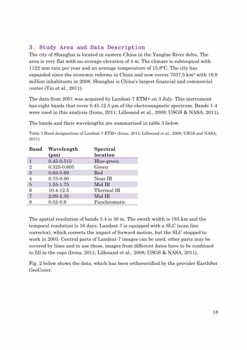
3. Study Area and Data Description The city of Shanghai is located in eastern China in the Yangtze River delta. The area is very flat with an average elevation of 4 m. The climate is subtropical with 1122 mm rain per year and an average temperature of 15.8°C. The city has expanded since the economic reforms in China and now covers 7037.5 km2 with 18.9 million inhabitants in 2008. Shanghai is China’s largest financial and commercial center (Yin et al., 2011).

The data from 2001 was acquired by Landsat-7 ETM+ on 3 July. This instrument has eight bands that cover 0.45-12.5 μm of the electromagnetic spectrum. Bands 1-4 were used in this analysis (Irons, 2011; Lillesand et al., 2008; USGS & NASA, 2011).

The bands and their wavelengths are summarized in table 3 below.

Table 3 Band designations of Landsat-7 ETM+ (Irons, 2011; Lillesand et al., 2008; USGS and NASA, 2011)

Band Wavelength (μm)

Spectral location

1 0.45-0.515 Blue-green 2 0.525-0.605 Green 3 0.63-0.69 Red 4 0.75-0.90 Near IR 5 1.55-1.75 Mid IR 6 10.4-12.5 Thermal IR 7 2.09-2.35 Mid IR 8 0.52-0.9 Panchromatic

The spatial resolution of bands 1-4 is 30 m. The swath width is 183 km and the temporal resolution is 16 days. Landsat-7 is equipped with a SLC (scan line corrector), which corrects the impact of forward motion, but the SLC stopped to work in 2003. Central parts of Landsat-7 images can be used, other parts may be covered by lines and to use these, images from different dates have to be combined to fill in the caps (Irons, 2011; Lillesand et al., 2008; USGS & NASA, 2011).

Fig. 2 below shows the data, which has been orthorectified by the provider EarthSat GeoCover.

19

Figure 2 Landsat-7 ETM+ 2001 image

The data from 2010 was acquired by the Chinese satellite HJ-1B on 30 July; this satellite is equipped with a CCD (charge-coupled device) camera and a hyperspectral imager. The data used in this project comes from the CCD camera. This camera has four bands that cover 0.43-0.9 μm of the electromagnetic spectrum and each of the bands has 30 m spatial resolution. The swath width is 700 km and its repetition cycle is four days. The HJ satellites are used for disaster monitoring and environment protection in China (CRESDA, 2009; Wang et al, 2005; Lillesand et al., 2008).

The bands and their wavelengths are summarized in table 4 below.

20

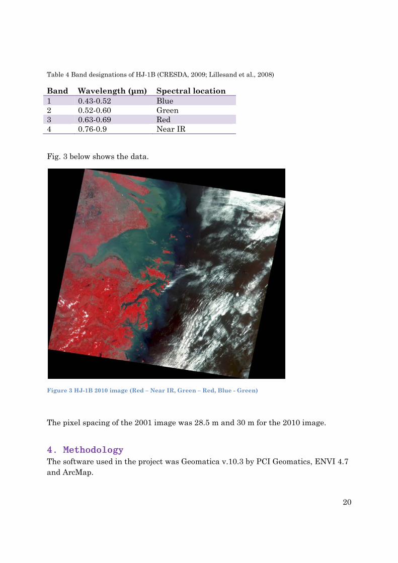
Table 4 Band designations of HJ-1B (CRESDA, 2009; Lillesand et al., 2008)

Band Wavelength (μm) Spectral location 1 0.43-0.52 Blue 2 0.52-0.60 Green 3 0.63-0.69 Red 4 0.76-0.9 Near IR

Fig. 3 below shows the data.

Figure 3 HJ-1B 2010 image (Red – Near IR, Green – Red, Blue - Green)

The pixel spacing of the 2001 image was 28.5 m and 30 m for the 2010 image.

4. Methodology The software used in the project was Geomatica v.10.3 by PCI Geomatics, ENVI 4.7 and ArcMap.

21

4.1 Geometric and Radiometric Correction The images were co-registered to each other using ground control points (GCPs). Seventeen GCPs were collected and the number of GCPs was reduced to ten to achieve an acceptable RMS error. The RMS error was 0.44. The X RMS error was 0.36 and the Y RMS error was 0.25. The images were resampled with cubic convolution (3). Both of the images’ pixel spacing was set to 30 m.

The images were then atmospherically corrected using calibration files in the software (Geomatica v.10.3). The Landsat-7 ETM+ image (Date 1) was calibrated using an ETM+ calibration file. Because HJ-1B is a new satellite, there was not any calibration file in the software and a calibration file for Landsat-4/5 TM was chosen, even though there is a difference in the spectrum covered. According to Lillesand et al (2008) the wavelength of the blue band of TM is 0.45-0.52 μm, resulting in a 0.02 μm difference, the other bands cover the same portions of the electromagnetic spectrum.

The HJ-1B image (Date 2) was a bit noisy, so a 3x3 average filter was applied on this image.

Radiometric correction was performed on the images using pseudo-invariant features (PIFs) that produce equations (4) for linear regression normalization. A rooftop and part of a lake were used as PIFs. Google maps of Shanghai were used as reference to verify the nature of the features. The resulting equations with correlation coefficients are listed in table 5 below.

Table 5 Equations for linear regression and correlation coefficients.

Band Equation Correlation coefficient Band 1 0.15x+25.10 0.96 Band 2 0.34x+63.40 0.96 Band 3 0.46x+44.23 0.97 Band 4 0.61x+41.48 0.98

Date 1 was used as the base image and Date 2 was the target image (x=respective band of Date 2), because it was of poor quality.

4.2 Image Differencing The algorithm was used with band 2 (green), band 3 (red) and band 4 (near IR).

The difference image d was produced by applying the following equation (an adaptation of (6)) to all pixel values in respective band of the images:

22

2 1 11

The difference image d was classified using unsupervised k-means classification, with k =12 for band 3, k =20 for band 4 and k =25 for band 2. This classification image was then visually inspected to identify classes of change and no-change with help of the corrected HJ-1B and Landsat-7 ETM+ images. These classes were then aggregated into one Change class and one No-change class. Some clusters were only made up of clouds; these were labeled as no change.

4.3 Post-Classification Comparison Each image was classified using supervised classification (maximum likelihood classification). Training areas were selected that represented the spectral signatures of each class. In Date 2 six classes could be identified; two urban classes, two water classes and two agriculture classes. These classes were later aggregated into three classes: Urban, Water and Agriculture. In Date 1 three urban classes, three water classes and four agriculture classes could be identified. These were also later aggregated into three classes: Urban, Water and Agriculture.

Image differencing was then performed with the aggregated classification images, using the following equation (an adaptation of (6)) applied to all pixel values:

2 1 12

The image d was then compared with the corrected HJ-1B and Landsat-7 ETM+ images in order to create the final change detection map with one Change and one No-change class. The final change detection map was filtered using a 5x5 median filter to reduce noise.

4.4 Accuracy Assessment Validation areas that represent change and no-change classes were selected by visually inspecting the corrected images. The final change detection maps were then compared pixel-by-pixel with the validation areas, in order to see if the algorithms managed to detect change.

For change, 1483 validation pixels were selected and for no-change, 1391 validation pixels were selected.

5. Results and Discussion All figures of the results are shown in Appendix A. In all final change detection maps, pink indicates change and black indicates no change. Figures 4-12 are false color composites (Red – Near IR, Green – Red, Blue - Green).

23

The overall impression of the result from both algorithms is that too much change has been detected. The result of Yin et al (2011) shows that the city of Shanghai has grown tremendously since 1979 but the expansion has slowed down in 2000-2009.

Fig. 4 below shows a section of downtown Shanghai.

Figure 4 Section of downtown Shanghai, left: Date 2, right: Date 1, the cross indicate a changed area

After geometric and atmospheric correction, the images were clipped to cover the same geographical area. The result of this is shown in fig. A and fig. B.

5.1. Change Detection using Image Differencing As an illustration of how the result of k-means classification of the difference image looks, the classified difference image of band 3 is shown in fig. C. The final change detection maps of image differencing are shown in fig. D (band 3), fig. E (band 2) and fig. F (band 4).

Image differencing with band 4 managed to detect some change along the coastline, but did not detect the new urban areas. This is illustrated in fig. 5 where the change detection (blue) is draped over Date 1. An undetected area is marked with a yellow cross.

Figure 5 Image differencing with band 4 draped over urban section of Date 1

24

Image differencing with band 3 did detect some change in the new urban areas, but did not detect much of the change occurring on the coastline. This is illustrated in fig. 6 below. Some of the area marked by the yellow cross was detected.


Image differencing with band 2 only detected some pixels of change along the coastline and in the new urban areas. This is illustrated in fig. 7. A part of the area marked by the yellow cross was detected.


Image differencing had problems identifying the new islands in the upper right corner. The new islands can clearly be seen if Date 1 and Date 2 are visually inspected, shown in fig. 8.

25

Figure 8 New islands, left: Date 2, right: Date 1

Image differencing with band 4 (fig. F in Appendix A) managed to identify the change, as did image differencing with band 2 (fig. E in Appendix A) but to a lesser degree, image differencing with band 3 (fig. D in Appendix A) failed to detect this change all together. The reason for Band 3 failing to detect this change could be that during the identification of change and no change in the classified difference image, too many pixels located in the sea were labeled as no change.

Another thing the difference images of the different bands identified differently was the presence of some kind of water reservoir or land fill in the middle of images. This can be seen easily when visually inspecting the corrected satellite images, as illustrated in fig. 9.

Figure 9 Water reservoir or landfill, left: Date 2, right: Date 1

Band 2 and 4 managed to identify this feature (fig. E and F in Appendix A), while it was undetected in band 3 (fig. D in Appendix A). The change detection in band 2 and 4 is illustrated below in fig. 10. The change detection is draped over the corrected Landsat-7 ETM+ image.

26

Figure 10 Left: image differencing band 2, right: image differencing band 4

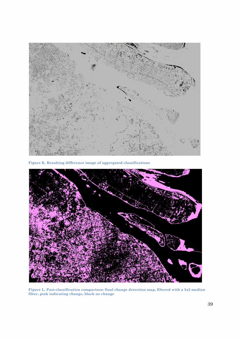
5.2 Change Detection using Post-Classification Comparison The result of the supervised classification of Date 2 and Date 1 is shown in fig. G and fig. H. The resulting aggregation of the classifications is shown in fig. I and fig. J. The resulting difference image is shown in fig. K. The final change detection map is shown in fig. L.

Post-classification comparison detected most of the change along the coastline and most of the change of the new urban areas. This is illustrated in fig. 11 below. The area marked by the yellow cross was fully detected.

Figure 11 Post-classification comparison draped over urban section of Date 1

The post-classification comparison managed to identify the new islands and the border of the landfill/water reservoir. This is illustrated in the following figure (fig. 12).

27

Figure 12 Post-classification comparison, left: new islands, right: water reservoir or landfill

5.2 Accuracy Assessment

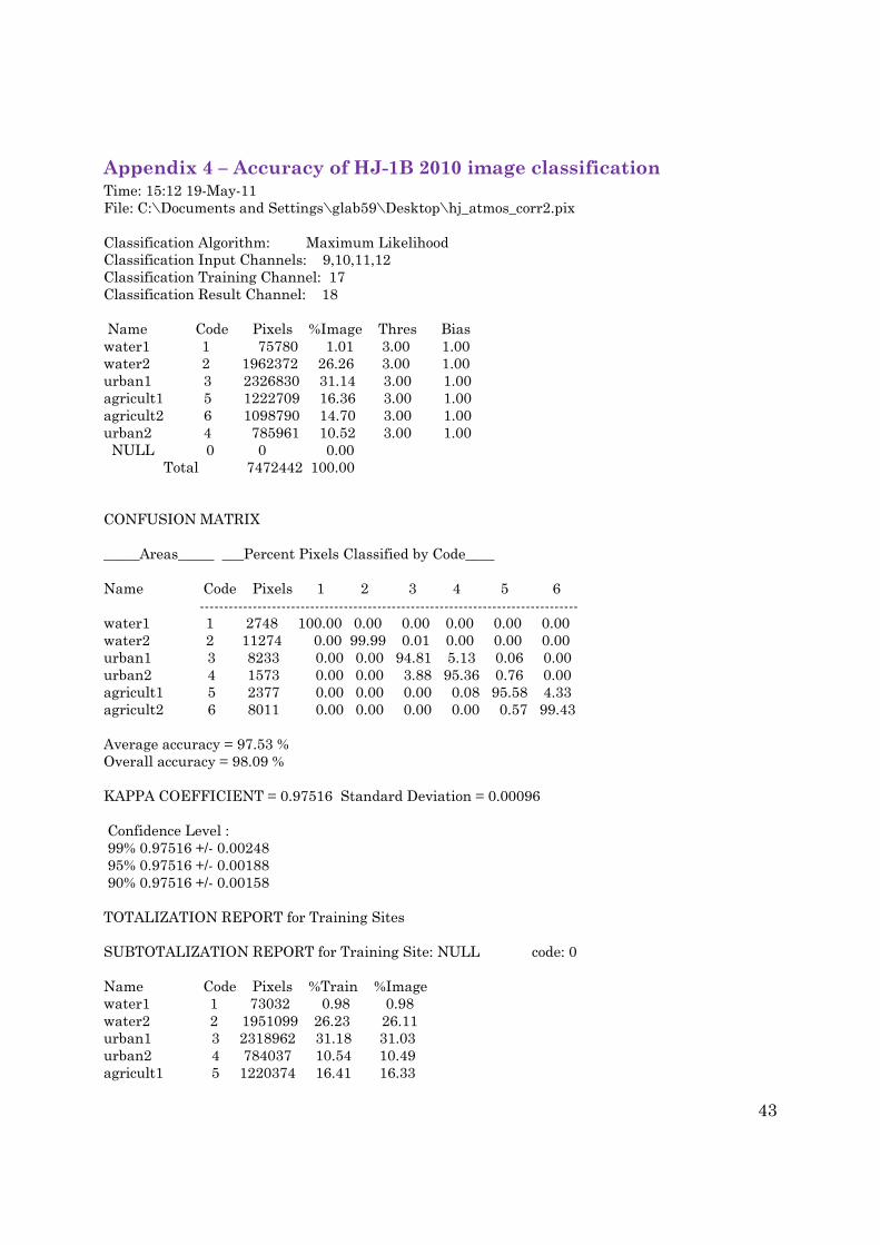
5.2.1 Classifications For HJ-1B, the overall accuracy was 98.09% and the average accuracy was 97.53%. The accuracy and confusion matrix of the HJ-1B classification are shown in Appendix 4. The separability matrix is shown in Appendix 5. For Landsat-7 ETM+, the overall accuracy was 87.54% and the average accuracy was 87.81%. The accuracy and confusion matrix of this classification is shown in Appendix 6. The separability matrix is shown in Appendix 7.

Agriculture proved to be a difficult class to classify in the supervised classification of the Landsat-7 ETM+ image, several more classes had to be used compared with the HJ-1B image. This resulted in a more grainy classification, as shown in fig. H in Appendix A. The separability matrix of the classification of the Landsat ETM+ image in Appendix 7 shows that two classes of agriculture (agricult3 and agricult 4) were the least separable. Date 1 had a better overall accuracy of the classification than Date 2. The post-classification comparison could have fared even better if the classification was a bit better.

When performing the visual inspection of the k-means unsupervised classification of the difference images, the situation of having to choose between two evils often occurred. Either some changed pixels were suppressed, because the majority of the cluster represented no change, or some unchanged pixels were labeled as changed, because most of the cluster represented change.

5.2.2 Change Detection Post-classification comparison performed with an accuracy of 90.96% and image differencing performed with an accuracy of about 25-47%. The accuracy is summarized in table 6 below.

28

Table 6 Overall accuracy of the algorithms

Algorithm Accuracy Image differencing with Band 2 24.07% Image differencing with Band 3 25.96% Image differencing with Band 4 46.93% Post-classification comparison 90.96%

The accuracies listed in the table above are overall accuracies; the evaluation of the performance of the algorithms must also take into consideration misclassification of change and no change to fully appreciate the performance of each algorithm (Yuan and Elvidge, 1998). Tables 7-10 contain this information.

Table 7 Image differencing Band 2

Class Change No change Change 24.1% 7.9% No change 75.9% 92.1%





Table 10 Post-classification comparison


Reports of the assessment are included in Appendix VI-IX.

From table 7 it can be seen that image differencing with band 2 had a low rate of misses (7.9%), but a substantially higher rate of false alarms (75.9%). The rate of

29

true positives were quite low (24.1%), but the rate of true negatives was very high (92.1%).

From table 8 it can be seen that image differencing with band 3 had a quite low rate of misses (16.1%), but a very high rate of false alarms (74.0%). The rate of true positives was quite low (26.0%), but the rate of true negatives was high (83.9%).

From table 9 it can be seen that image differencing with band 4 had a low rate of misses (11.3%) but a high rate of false alarms (53.1%). The rate of true positives was quite high (46.9%) and the rate of true negatives 88.7% was high.

From table 10 it can be seen that post-classification comparison had a low rate of misses (9.0%), but a higher rate of false alarms (29.3%). This algorithm had high rates of true positives and negatives (91.0% and 70.7%).

The best algorithm should have about equal rates of true positives and true negatives. Post-classification comparison achieves this. The worst algorithm has a high rate of false alarms, meaning overestimating the change. Image differencing with band 2 has the highest rate of false alarms, which a visual inspection of the final change detection map should verify.

30

6. Conclusions Image differencing is not a suitable algorithm for images from different sensors, because the change detection has low accuracy. A more suitable algorithm is post-classification comparison, because of its higher accuracy.

The major disadvantage of the methodology of both algorithms is that it is subject to a great deal of visual inspection and hence relies heavily on the analyst’s skill and honesty. It is also difficult to repeat.

Further research is needed on how to utilize images from different sensors.

31

7. References CRESDA, 2009. Technical specification of payloads of HJ-1A/1B/1C. Available online at: http://www.cresda.com/n16/n92006/n92066/n98627/index.html (last accessed 9 June 2011)

Du, Y., Teillet, P.M. & Cihlar, J., 2002. Radiometric normalization of multitemporal high-resolution satellite images with quality control for land cover change detection. Remote Sensing of Environment, 82:123-134.

Duda, T & Canty, M., 2002. Unsupervised classification of satellite imagery: choosing a good algorithm. International Journal of Remote Sensing, 33:11, 2193-2212.

Gomez-Chova, L., Fernández-Prieto, D., Calpe, J., Soria, E., Vila, J. & Camps-Valls, G., 2006. Urban monitoring using mult-temporal SAR and multi-spectral data. Pattern Recognition Letters, 27: 234-243.

Griffiths, P., Hostert P., Gruebner, O., & van der Linden, S., 2010. Mapping megacity growth with multi-sensor data. Remote Sensing of Environment, 114:426-439.

Irons, J.R., 2011. The Enhanced Thematic Mapper Plus. Available online at: http://landsat.gsfc.nasa.gov/about/etm+.html (last accessed 1 June 2011)

Jensen, J.R., 2005. Introductory Digital Image Processing – A Remote Sensing Perspective. 3rd ed. Upper Saddle River: Pearson Prentice Hall.

Johnson, R.D. & Kasischke, E.S., 1998. Change vector analysis: A technique for the multispectral monitoring of land cover and condition. International Journal of Remote Sensing, 19:3, 411-426.

Keys, R.G., 1981. Cubic Convolution Interpolation for Digital Image Processing. IEEE Transactions on Acoustics, Speech and Signal Processing, 29:6, 1153 – 1160.

Kontoes, C.C., 2008. Operational land cover change detection using change vector analysis. International Journal of Remote Sensing, 29:16, 4757-4779.

Lambin, E.F & Strahler, A.H., 1994. Change Vector Analysis in Multitemporal Space: A Tool to Detect and Categorize Land-Cover Change Processes Using High Temporal-Resolution Satellite Data. Remote Sensing of Environment, 48:231-244.

32

Li, X. & Yeh, A.G.-O., 2004. Analyzing spatial restructuring of land use patterns in a fast growing region using remote sensing and GIS. Landscape and Urban Planning, 69:335-354.

Lillesand, T.M., Kiefer, R.W. & Chipman, J.W., 2008. Remote Sensing and Image Interpretation. 6th ed. Hoboken: John Wiley & Sons.

Liu, Y., Nishiyama, S. & Yano, T., 2004. Analysis of four change detection algorithms in bi-temporal space with a case study. International Journal of Remote Sensing, 25;11, 2121-2139.

Lu, D., Mausel, P., Brondízio, E. & Moran, E., 2004. Change detection techniques; International Journal of Remote Sensing, 25:12, 2365-2407.

PCI Geomatics, 2011. Geomatica Help – Testing signature separability.

Prakash, A & Gupta, R.P., 1998. Land-use mapping and change detection in the Jharia coalfield. International Journal of Remote Sensing, 19:3, 391-410.

Radke, R.J, Andra, S., Al-Kofahi, O. & Roysam, B., 2005. Image Change Detection Algorithms: A Systematic Survey. IEEE Transactions on Image Processing, 14:3, 294-307.

Ridd, M.K. & Liu, J., 1998. A Comparison of Four Algorithms for Change Detection in an Urban Environment. Remote Sensing of Environment, 63:95-100, 1998.

Singh, A., 1989. Review Article Digital change detection techniques using remotely-sensed data. International Journal of Remote Sensing, 10:6, 989-1003.

USGS & NASA, 2011. Landsat: A Global Land-Imaging Project. Available online at: http://pubs.usgs.gov/fs/2010/3026/pdf/FS2010-3026.pdf (last accessed 1 June 2011)

Wang, X., Wang, G., Guan, Y., Chen, Q., & Gao, L., 2005. Small Satellite Constellation for Disaster Monitoring in China. Geoscience and Remote Sensing Symposium IEEE Proceedings.

Yang, X. & Lo, C.P., 2000. Relative Radiometric Normalization Performance for Change Detection from Multi-Date Satellite Images. Photogrammetric Engineering & Remote Sensing, 66:8, 967-980.

Yin, J., Yin, Z., Zhong, H., Xu, S., Hu, X., Wang, J. & Wu, J., 2011. Monitoring urban expansion and land use/land cover changes of Shanghai metropolitan area

33

during the transitional economy (1979–2009) in China. Environmental Monitoring and Assessment, 177:609-621.

Yuan, D. & Elvidge, C., 1998. NALC Land Cover Change Detection Pilot Study: Washington D.C. Area Experiments. Remote Sensing of Environment, 66:166-178.

34

8. Appendices

Appendix A – The Result

Figure A. Landsat-7 ETM+ 2001 image after corrections (Red – Near IR, Green – Red, Blue - Green)

Figure B. HJ-1B 2010 image after corrections (Red – Near IR, Green – Red, Blue - Green)

35

Figure C. k-means classification of difference image (band 3)

Figure D. Image differencing with band 3: final change detection map, pink indicating change, black no change

36

Figure E. Image differencing with band 2: final change detection map, pink indicating change, black no change

Figure F. Image differencing with band 4: final change detection map, pink indicating change, black no change

37

Figure G. Supervised classification of HJ-1B 2010 image

Figure H. Supervised classification of Landsat-7 ETM+ 2001 image

38

Figure I. Aggregation of classes – HJ-1B 2010 image, pink – urban, yellow – agriculture, blue water

Figure J. Aggregation of classes – Landsat-7 ETM+ 2001 image, same color scheme as fig. I

39

Figure K. Resulting difference image of aggregated classifications

Figure L. Post-classification comparison: final change detection map, filtered with a 5x5 median filter, pink indicating change, black no change

40

Appendix 1 – Result of K-means Classification – Band 3 Time: 18:35 20-May-11 File: C:\Documents and Settings\glab59\Desktop\Copy of im_diff_band3.pix Classification Algorithm: K-Means Unsupervised Classification Input Channels: 1 Classification Result Channel: 2 Number of Clusters: 12 Cluster Pixels Mean Std Dev : ( 1) 963976 3.36174 3.14229 ( 2) 1405386 14.42514 3.51411 ( 3) 1548604 25.92842 3.05773 ( 4) 1163375 36.60860 2.89786 ( 5) 1019565 45.46129 2.27589 ( 6) 696225 52.76139 1.98171 ( 7) 396600 59.58850 1.96368 ( 8) 202158 67.14455 2.48515 ( 9) 59207 76.28130 2.68737 ( 10) 13845 87.61546 4.14735 ( 11) 2619 107.15235 6.10348 ( 12) 882 130.81633 7.78278 -------- Total 7472442

Appendix 2 – Result of K-means Classification – Band 2 Time: 14:45 24-May-11 File: C:\Documents and Settings\glab59\Desktop\im_diff_band2.pix Classification Algorithm: K-Means Unsupervised Classification Input Channels: 1 Classification Result Channel: 4 Number of Clusters: 25 Cluster Pixels Mean Std Dev : ( 1) 113987 0.15991 0.49359

41

( 2) 44806 5.65076 1.70126 ( 3) 75379 12.24442 1.99638 ( 4) 137500 19.09487 1.67790 ( 5) 432101 24.41623 1.34674 ( 6) 649785 29.03064 1.41758 ( 7) 869831 34.54704 1.71621 ( 8) 841355 40.03166 1.40561 ( 9) 980110 45.43530 1.70472 ( 10) 913367 51.53228 1.71381 ( 11) 799081 56.99409 1.41094 ( 12) 840423 62.35413 1.69324 ( 13) 440092 67.75704 1.39501 ( 14) 210060 72.64682 1.38085 ( 15) 80361 77.59294 1.37297 ( 16) 28375 82.58626 1.37508 ( 17) 9782 87.59558 1.38071 ( 18) 3759 93.12051 1.88485 ( 19) 1062 100.48211 1.95937 ( 20) 468 107.33974 1.65184 ( 21) 283 113.02120 1.44618 ( 22) 210 117.94286 1.40968 ( 23) 157 123.09554 1.48789 ( 24) 75 129.73333 1.94136 ( 25) 33 136.60606 2.80626 -------- Total 7472442

42

Appendix 3 – Result of K-means Classification – Band 4 Time: 13:33 24-May-11 File: C:\Documents and Settings\glab59\Desktop\im_diff_band4.pix Classification Algorithm: K-Means Unsupervised Classification Input Channels: 1 Classification Result Channel: 4 Number of Clusters: 20 Cluster Pixels Mean Std Dev : ( 1) 322812 0.78401 1.52272 ( 2) 248974 10.92641 2.84745 ( 3) 398065 20.83734 2.85995 ( 4) 543277 30.37287 2.59387 ( 5) 1085103 39.02242 2.19262 ( 6) 1289060 46.80330 2.61056 ( 7) 1292975 56.05417 2.56323 ( 8) 853595 64.41063 2.55630 ( 9) 548325 74.28267 2.87682 ( 10) 382198 83.78185 2.56848 ( 11) 239119 92.24011 2.27053 ( 12) 143198 100.07846 2.25310 ( 13) 69249 107.96510 2.25367 ( 14) 35950 116.56473 2.78810 ( 15) 11281 126.32355 2.52359 ( 16) 5508 135.93991 2.83295 ( 17) 2277 145.03338 2.28949 ( 18) 1137 153.14776 2.48428 ( 19) 297 162.24242 2.75397 ( 20) 42 178.11905 6.94263 -------- Total 7472442

43

Appendix 4 – Accuracy of HJ-1B 2010 image classification Time: 15:12 19-May-11 File: C:\Documents and Settings\glab59\Desktop\hj_atmos_corr2.pix Classification Algorithm: Maximum Likelihood Classification Input Channels: 9,10,11,12 Classification Training Channel: 17 Classification Result Channel: 18 Name Code Pixels %Image Thres Bias water1 1 75780 1.01 3.00 1.00 water2 2 1962372 26.26 3.00 1.00 urban1 3 2326830 31.14 3.00 1.00 agricult1 5 1222709 16.36 3.00 1.00 agricult2 6 1098790 14.70 3.00 1.00 urban2 4 785961 10.52 3.00 1.00 NULL 0 0 0.00 Total 7472442 100.00 CONFUSION MATRIX _____Areas_____ ___Percent Pixels Classified by Code____ Name Code Pixels 1 2 3 4 5 6 ------------------------------------------------------------------------------- water1 1 2748 100.00 0.00 0.00 0.00 0.00 0.00 water2 2 11274 0.00 99.99 0.01 0.00 0.00 0.00 urban1 3 8233 0.00 0.00 94.81 5.13 0.06 0.00 urban2 4 1573 0.00 0.00 3.88 95.36 0.76 0.00 agricult1 5 2377 0.00 0.00 0.00 0.08 95.58 4.33 agricult2 6 8011 0.00 0.00 0.00 0.00 0.57 99.43 Average accuracy = 97.53 % Overall accuracy = 98.09 % KAPPA COEFFICIENT = 0.97516 Standard Deviation = 0.00096 Confidence Level : 99% 0.97516 +/- 0.00248 95% 0.97516 +/- 0.00188 90% 0.97516 +/- 0.00158 TOTALIZATION REPORT for Training Sites SUBTOTALIZATION REPORT for Training Site: NULL code: 0 Name Code Pixels %Train %Image water1 1 73032 0.98 0.98 water2 2 1951099 26.23 26.11 urban1 3 2318962 31.18 31.03 urban2 4 784037 10.54 10.49 agricult1 5 1220374 16.41 16.33

44

agricult2 6 1090722 14.66 14.60 ----------------------------------------------------- Totals 7438226 100.00 99.54 SUBTOTALIZATION REPORT for Training Site: water1 code: 1 Name Code Pixels %Train %Image water1 1 2748 100.00 0.04 ----------------------------------------------------- Totals 2748 100.00 0.04 SUBTOTALIZATION REPORT for Training Site: water2 code: 2 Name Code Pixels %Train %Image water2 2 11273 99.99 0.15 urban1 3 1 0.01 0.00 ----------------------------------------------------- Totals 11274 100.00 0.15 SUBTOTALIZATION REPORT for Training Site: urban1 code: 3 Name Code Pixels %Train %Image urban1 3 7806 94.81 0.10 urban2 4 422 5.13 0.01 agricult1 5 5 0.06 0.00 ----------------------------------------------------- Totals 8233 100.00 0.11 SUBTOTALIZATION REPORT for Training Site: urban2 code: 4 Name Code Pixels %Train %Image urban1 3 61 3.88 0.00 urban2 4 1500 95.36 0.02 agricult1 5 12 0.76 0.00 ----------------------------------------------------- Totals 1573 100.00 0.02 SUBTOTALIZATION REPORT for Training Site: agricult1 code: 5 Name Code Pixels %Train %Image urban2 4 2 0.08 0.00 agricult1 5 2272 95.58 0.03 agricult2 6 103 4.33 0.00 ----------------------------------------------------- Totals 2377 100.00 0.03 SUBTOTALIZATION REPORT for Training Site: agricult2 code: 6 Name Code Pixels %Train %Image agricult1 5 46 0.57 0.00 agricult2 6 7965 99.43 0.11 ----------------------------------------------------- Totals 8011 100.00 0.11

45

Appendix 5 – Separability Matrix for Classification of HJ-1B 2010 image

46

Appendix 6 – Accuracy of Landsat-7 ETM+ 2001 image Classification Time: 09:12 23-May-11 File: C:\Documents and Settings\glab59\Desktop\hj_atmos_corr2.pix Classification Algorithm: Maximum Likelihood Classification Input Channels: 5,6,7,8 Classification Training Channel: 21 Classification Result Channel: 22 Name Code Pixels %Image Thres Bias water1 1 67229 0.90 3.00 1.00 water2 2 2290345 30.65 3.00 1.00 water3 3 34870 0.47 3.00 1.00 urban1 4 1230120 16.46 3.00 1.00 urban2 5 4501 0.06 3.00 1.00 urban3 6 97638 1.31 3.00 1.00 agricult1 7 87453 1.17 3.00 1.00 agricult2 8 445896 5.97 3.00 1.00 agricult3 9 2159348 28.90 3.00 1.00 agricult4 10 1055042 14.12 3.00 1.00 NULL 0 0 0.00 Total 7472442 100.00 CONFUSION MATRIX _____Areas_____ ___Percent Pixels Classified by Code____ Name Code Pixels 1 2 3 4 5 6 7 8 9 ---------------------------------------------------------------------------------------------------------- water1 1 215 96.74 0.00 1.40 0.00 0.00 0.00 0.00 0.00 1.86 water2 2 6957 0.00 97.20 0.00 2.37 0.00 0.42 0.00 0.00 0.01 water3 3 557 0.36 1.62 95.87 0.90 0.00 0.00 0.00 0.00 0.36 urban1 4 573 0.00 0.00 0.00 77.49 0.00 3.84 0.00 0.52 10.12 urban2 5 168 0.00 0.00 0.00 0.00 100.00 0.00 0.00 0.00 0.00 urban3 6 104 0.00 0.00 0.00 0.00 0.00 100.00 0.00 0.00 0.00 agricult1 7 423 0.00 0.00 0.00 0.00 0.00 0.00 94.80 2.36 0.00 agricult2 8 478 0.00 0.00 0.00 0.00 0.00 0.00 2.30 83.26 14.23 agricult3 9 2065 0.29 0.00 0.15 4.99 0.00 0.00 0.34 14.38 57.58 agricult4 10 856 0.00 0.00 0.00 7.59 0.00 0.00 0.82 6.54 9.93 Name Code Pixels 10 ---------------------------------- water1 1 215 0.00 water2 2 6957 0.00 water3 3 557 0.90 urban1 4 573 8.03 urban2 5 168 0.00 urban3 6 104 0.00 agricult1 7 423 2.84 agricult2 8 478 0.21

47

agricult3 9 2065 22.28 agricult4 10 856 75.12 Average accuracy = 87.81 % Overall accuracy = 87.54 % KAPPA COEFFICIENT = 0.81088 Standard Deviation = 0.00422 Confidence Level : 99% 0.81088 +/- 0.01088 95% 0.81088 +/- 0.00826 90% 0.81088 +/- 0.00694 TOTALIZATION REPORT for Training Sites SUBTOTALIZATION REPORT for Training Site: NULL code: 0 Name Code Pixels %Train %Image water1 1 67013 0.90 0.90 water2 2 2283574 30.61 30.56 water3 3 34330 0.46 0.46 urban1 4 1229338 16.48 16.45 urban2 5 4333 0.06 0.06 urban3 6 97483 1.31 1.30 agricult1 7 87027 1.17 1.16 agricult2 8 445132 5.97 5.96 agricult3 9 2157941 28.93 28.88 agricult4 10 1053875 14.13 14.10 ----------------------------------------------------- Totals 7460046 100.00 99.83 SUBTOTALIZATION REPORT for Training Site: water1 code: 1 Name Code Pixels %Train %Image water1 1 208 96.74 0.00 water3 3 3 1.40 0.00 agricult3 9 4 1.86 0.00 ----------------------------------------------------- Totals 215 100.00 0.00 SUBTOTALIZATION REPORT for Training Site: water2 code: 2 Name Code Pixels %Train %Image water2 2 6762 97.20 0.09 urban1 4 165 2.37 0.00 urban3 6 29 0.42 0.00 agricult3 9 1 0.01 0.00 ----------------------------------------------------- Totals 6957 100.00 0.09 SUBTOTALIZATION REPORT for Training Site: water3 code: 3

48

Name Code Pixels %Train %Image water1 1 2 0.36 0.00 water2 2 9 1.62 0.00 water3 3 534 95.87 0.01 urban1 4 5 0.90 0.00 agricult3 9 2 0.36 0.00 agricult4 10 5 0.90 0.00 ----------------------------------------------------- Totals 557 100.00 0.01 SUBTOTALIZATION REPORT for Training Site: urban1 code: 4 Name Code Pixels %Train %Image urban1 4 444 77.49 0.01 urban3 6 22 3.84 0.00 agricult2 8 3 0.52 0.00 agricult3 9 58 10.12 0.00 agricult4 10 46 8.03 0.00 ----------------------------------------------------- Totals 573 100.00 0.01 SUBTOTALIZATION REPORT for Training Site: urban2 code: 5 Name Code Pixels %Train %Image urban2 5 168 100.00 0.00 ----------------------------------------------------- Totals 168 100.00 0.00 SUBTOTALIZATION REPORT for Training Site: urban3 code: 6 Name Code Pixels %Train %Image urban3 6 104 100.00 0.00 ----------------------------------------------------- Totals 104 100.00 0.00 SUBTOTALIZATION REPORT for Training Site: agricult1 code: 7 Name Code Pixels %Train %Image agricult1 7 401 94.80 0.01 agricult2 8 10 2.36 0.00 agricult4 10 12 2.84 0.00 ----------------------------------------------------- Totals 423 100.00 0.01 SUBTOTALIZATION REPORT for Training Site: agricult2 code: 8 Name Code Pixels %Train %Image agricult1 7 11 2.30 0.00 agricult2 8 398 83.26 0.01 agricult3 9 68 14.23 0.00 agricult4 10 1 0.21 0.00 ----------------------------------------------------- Totals 478 100.00 0.01

49

SUBTOTALIZATION REPORT for Training Site: agricult3 code: 9 Name Code Pixels %Train %Image water1 1 6 0.29 0.00 water3 3 3 0.15 0.00 urban1 4 103 4.99 0.00 agricult1 7 7 0.34 0.00 agricult2 8 297 14.38 0.00 agricult3 9 1189 57.58 0.02 agricult4 10 460 22.28 0.01 ----------------------------------------------------- Totals 2065 100.00 0.03 SUBTOTALIZATION REPORT for Training Site: agricult4 code: 10 Name Code Pixels %Train %Image urban1 4 65 7.59 0.00 agricult1 7 7 0.82 0.00 agricult2 8 56 6.54 0.00 agricult3 9 85 9.93 0.00 agricult4 10 643 75.12 0.01 ----------------------------------------------------- Totals 856 100.00 0.01

Appendix 7 – Separability Matrix of Landsat-7 ETM+ 2001 Image Classification

50

Appendix 8 – Accuracy Assessment Report for Post-Classification Comparison Time of execution : 24-May-2011 11:39:08:577 1 MLR Maximum Likelihood Report V10.3 EASI/PACE 11:39 24May2011 Subarea Reports using theme channel 1 and subarea channel 2: 1 [ 8U] focus Imported from 1 on C:\Documents and Settings\glab524May2011 2 [ 8U] focus Empty 24May2011 Totalization Report for Subarea code: 0 Seg Name Code Pixels Sq. Kilometres %Subarea %Image 1 2099350 1889.41 28.11 28.09 Null 0 5370218 4833.20 71.89 71.87 ---------- ------------- ------ ------ Subarea totals 7469568 6722.61 100.00 99.96 Totalization Report for Subarea code: 1 Seg Name Code Pixels Sq. Kilometres %Subarea %Image 1 1349 1.21 90.96 0.02 Null 0 134 0.12 9.04 0.00 ---------- ------------- ------ ------ Subarea totals 1483 1.33 100.00 0.02 Totalization Report for Subarea code: 2 Seg Name Code Pixels Sq. Kilometres %Subarea %Image 1 408 0.37 29.33 0.01 Null 0 983 0.88 70.67 0.01 ---------- ------------- ------ ------ Subarea totals 1391 1.25 100.00 0.02 1 [ 8U] focus Imported from 1 on C:\Documents and Settings\glab524May2011 Totalization Report for theme channel: 1 Seg Name Code Pixels Sq. Kilometres %Image 1 2101107 1891.00 28.12 Null 0 5371335 4834.20 71.88

51

---------- ------------- ------ Image total ************* 6725.20 100.00 ________Areas_______ ___________Percent Pixels Classified by Code__________ Code Name Pixels 0 1 -------------------- ------------------------------------------------------- 1 1483 9.0 91.0 (Change) 2 1391 70.7 29.3 (No change) Average accuracy = 90.96% Overall accuracy = 90.96% Kappa Coefficient = 1.10452 Standard Deviation = NaN Confidence Level : 99% 1.10452 +/- NaN 95% 1.10452 +/- NaN 90% 1.10452 +/- NaN Execution Successful.

52

Appendix 9 – Accuracy Assessment Report for Image Differencing with Band 3 Time of execution : 23-May-2011 20:22:15:822 1 MLR Maximum Likelihood Report V10.3 EASI/PACE 20:22 23May2011 Subarea Reports using theme channel 1 and subarea channel 2: 1 [ 8U] focus Imported from 1 on C:\Documents and Settings\gla..23May2011 2 [ 8U] focus Empty 23May2011 Totalization Report for Subarea code: 0 Seg Name Code Pixels Sq. Kilometres %Subarea %Image 1 598149 538.33 8.01 8.00 Null 0 6871419 6184.28 91.99 91.96 ---------- ------------- ------ ------ Subarea totals 7469568 6722.61 100.00 99.96 Totalization Report for Subarea code: 1 Seg Name Code Pixels Sq. Kilometres %Subarea %Image 1 385 0.35 25.96 0.01 Null 0 1098 0.99 74.04 0.01 ---------- ------------- ------ ------ Subarea totals 1483 1.33 100.00 0.02 Totalization Report for Subarea code: 2 Seg Name Code Pixels Sq. Kilometres %Subarea %Image 1 224 0.20 16.10 0.00 Null 0 1167 1.05 83.90 0.02 ---------- ------------- ------ ------ Subarea totals 1391 1.25 100.00 0.02 1 [ 8U] focus Imported from 1 on C:\Documents and Settings\gla..23May2011 Totalization Report for theme channel: 1 Seg Name Code Pixels Sq. Kilometres %Image 1 598758 538.88 8.01 Null 0 6873684 6186.32 91.99

53

---------- ------------- ------ Image total ************* 6725.20 100.00 ________Areas_______ ___________Percent Pixels Classified by Code__________ Code Name Pixels 0 1 -------------------- ------------------------------------------------------- 1 1483 74.0 26.0 (Change) 2 1391 83.9 16.1 (No change) Average accuracy = 25.96% Overall accuracy = 25.96% Kappa Coefficient = 1.81140 Standard Deviation = NaN Confidence Level : 99% 1.81140 +/- NaN 95% 1.81140 +/- NaN 90% 1.81140 +/- NaN Execution Successful.

54

Appendix 10 – Accuracy Assessment Report for Image Differencing with Band 2 Time of execution : 24-May-2011 18:11:07:497 1 MLR Maximum Likelihood Report V10.3 EASI/PACE 18:11 24May2011 Subarea Reports using theme channel 1 and subarea channel 2:

1 [ 8U] focus Imported from 1 on C:\Documents and Settings\glab524May2011 2 [ 8U] focus Empty 24May2011 Totalization Report for Subarea code: 0 Seg Name Code Pixels Sq. Kilometres %Subarea %Image 1 1089206 980.29 14.58 14.58 Null 0 6380362 5742.33 85.42 85.39 ---------- ------------- ------ ------ Subarea totals 7469568 6722.61 100.00 99.96 Totalization Report for Subarea code: 1 Seg Name Code Pixels Sq. Kilometres %Subarea %Image 1 357 0.32 24.07 0.00 Null 0 1126 1.01 75.93 0.02 ---------- ------------- ------ ------ Subarea totals 1483 1.33 100.00 0.02 Totalization Report for Subarea code: 2 Seg Name Code Pixels Sq. Kilometres %Subarea %Image 1 110 0.10 7.91 0.00 Null 0 1281 1.15 92.09 0.02 ---------- ------------- ----- ------ Subarea totals 1391 1.25 100.00 0.02 1 [ 8U] focus Imported from 1 on C:\Documents and Settings\glab524May2011 Totalization Report for theme channel: 1 Seg Name Code Pixels Sq. Kilometres %Image 1 1089673 980.71 14.58 Null 0 6382769 5744.49 85.42 ---------- ------------- ------ Image total ************* 6725.20 100.00

55

________Areas_______ ___________Percent Pixels Classified by Code__________ Code Name Pixels 0 1 -------------------- ------------------------------------------------------- 1 1483 75.9 24.1 (Change) 2 1391 92.1 7.9 (No change) Average accuracy = 24.07% Overall accuracy = 24.07% Kappa Coefficient = 1.82671 Standard Deviation = NaN Confidence Level : 99% 1.82671 +/- NaN 95% 1.82671 +/- NaN 90% 1.82671 +/- NaN Execution Successful.

56

Appendix 11 – Accuracy Assessment Report for Image Differencing with Band 4 Time of execution : 24-May-2011 15:18:53:419 1 MLR Maximum Likelihood Report V10.3 EASI/PACE 15:18 24May2011 Subarea Reports using theme channel 1 and subarea channel 2: 1 [ 8U] focus Imported from 1 on C:\Documents and Settings\glab524May2011 2 [ 8U] focus Empty 24May2011 Totalization Report for Subarea code: 0 Seg Name Code Pixels Sq. Kilometres %Subarea %Image 1 1437389 1293.65 19.24 19.24 Null 0 6032179 5428.96 80.76 80.73 ---------- ------------- ------ ------ Subarea totals 7469568 6722.61 100.00 99.96 Totalization Report for Subarea code: 1 Seg Name Code Pixels Sq. Kilometres %Subarea %Image 1 696 0.63 46.93 0.01 Null 0 787 0.71 53.07 0.01 ---------- ------------- ------ ------ Subarea totals 1483 1.33 100.00 0.02 Totalization Report for Subarea code: 2 Seg Name Code Pixels Sq. Kilometres %Subarea %Image 1 157 0.14 11.29 0.00 Null 0 1234 1.11 88.71 0.02 ---------- ------------- ------ ------ Subarea totals 1391 1.25 100.00 0.02 1 [ 8U] focus Imported from 1 on C:\Documents and Settings\glab524May2011 Totalization Report for theme channel: 1 Seg Name Code Pixels Sq. Kilometres %Image 1 1438242 1294.42 19.25 Null 0 6034200 5430.78 80.75 ---------- ------------- ------ Image total ************* 6725.20 100.00

57

________Areas_______ ___________Percent Pixels Classified by Code__________ Code Name Pixels 0 1 -------------------- ------------------------------------------------------- 1 1483 53.1 46.9 (Change) 2 1391 88.7 11.3 (No change) Average accuracy = 46.93% Overall accuracy = 46.93% Kappa Coefficient = 1.58815 Standard Deviation = NaN Confidence Level : 99% 1.58815 +/- NaN 95% 1.58815 +/- NaN 90% 1.58815 +/- NaN Execution Successful.