multivariate analysis of genetic data: exploring group

Multivariate analysis of genetic data:exploring group diversity

Thibaut Jombart∗

Imperial College London

MRC Centre for Outbreak Analysis and Modelling

August 18, 2016

Abstract

This practical provides an introduction to the analysis of group diversity in geneticdata analysis using R . First, simple clustering methods are used to infer the nature, andthe number of genetic groups. Second, we show how group information can be used toexplore the genetic diversity using the Discriminant Analysis of Principal Components(DAPC). This second part will include two studies of the genetic makeup of Maripaulisnonsensicus populations, as well as an investigation of the origins of cattle allegedlyabducted by aliens.

∗[email protected]

1

Contents

1 Defining genetic clusters 31.1 Hierarchical clustering . . . . . . . . . . . . . . . . . . . . . . . . . . . . . . 31.2 K-means . . . . . . . . . . . . . . . . . . . . . . . . . . . . . . . . . . . . . . 6

2 Describing group diversity: Maripaulis nonsensicus populations 82.1 Maripaulis nonsensicus : first contact . . . . . . . . . . . . . . . . . . . . . . 82.2 Maripaulis nonsensicus : the return . . . . . . . . . . . . . . . . . . . . . . . 10

3 Describing group diversity: cattle breed discrimination and alienabductions 133.1 Choosing how many components to retain . . . . . . . . . . . . . . . . . . . 133.2 Using cross-validation . . . . . . . . . . . . . . . . . . . . . . . . . . . . . . . 163.3 Alien abductions . . . . . . . . . . . . . . . . . . . . . . . . . . . . . . . . . 19

4 To go further 24

2

1 Defining genetic clusters

Group information is not always known when analysing genetic data. Even when some priorclustering can be defined, it is not always obvious that these are the best genetic clustersthat can be defined. In this section, we illustrate two simple approaches for defining geneticclusters.

1.1 Hierarchical clustering

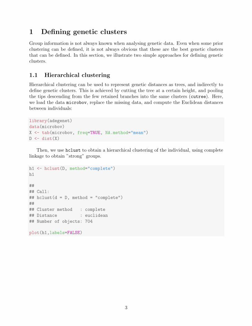
Hierarchical clustering can be used to represent genetic distances as trees, and indirectly todefine genetic clusters. This is achieved by cutting the tree at a certain height, and poolingthe tips descending from the few retained branches into the same clusters (cutree). Here,we load the data microbov, replace the missing data, and compute the Euclidean distancesbetween individuals:

library(adegenet)

data(microbov)

X <- tab(microbov, freq=TRUE, NA.method="mean")

D <- dist(X)

Then, we use hclust to obtain a hierarchical clustering of the individual, using completelinkage to obtain ”strong” groups.

h1 <- hclust(D, method="complete")

h1

##

## Call:

## hclust(d = D, method = "complete")

##

## Cluster method : complete

## Distance : euclidean

## Number of objects: 704

plot(h1,labels=FALSE)

3

23

45

6

Cluster Dendrogram

hclust (*, "complete")D

Hei

ght

Groups can be defined by cutting the tree at a given height. This is performed by thefunction cutree, which can also find the right height to obtain a specific number of clusters.Here, we first look at two groups:

grp <- cutree(h1, k=2)

head(grp,10)

## AFBIBOR9503 AFBIBOR9504 AFBIBOR9505 AFBIBOR9506 AFBIBOR9507 AFBIBOR9508

## 1 1 1 1 1 1

## AFBIBOR9509 AFBIBOR9510 AFBIBOR9511 AFBIBOR9512

## 1 1 1 1

The function table is extremely useful, as it can be used to build contingency tables.Here, we use it to compare the inferred groups to the species and the origins of the cattles.

table(grp, other(microbov)$spe)

##

## grp BI BT

4

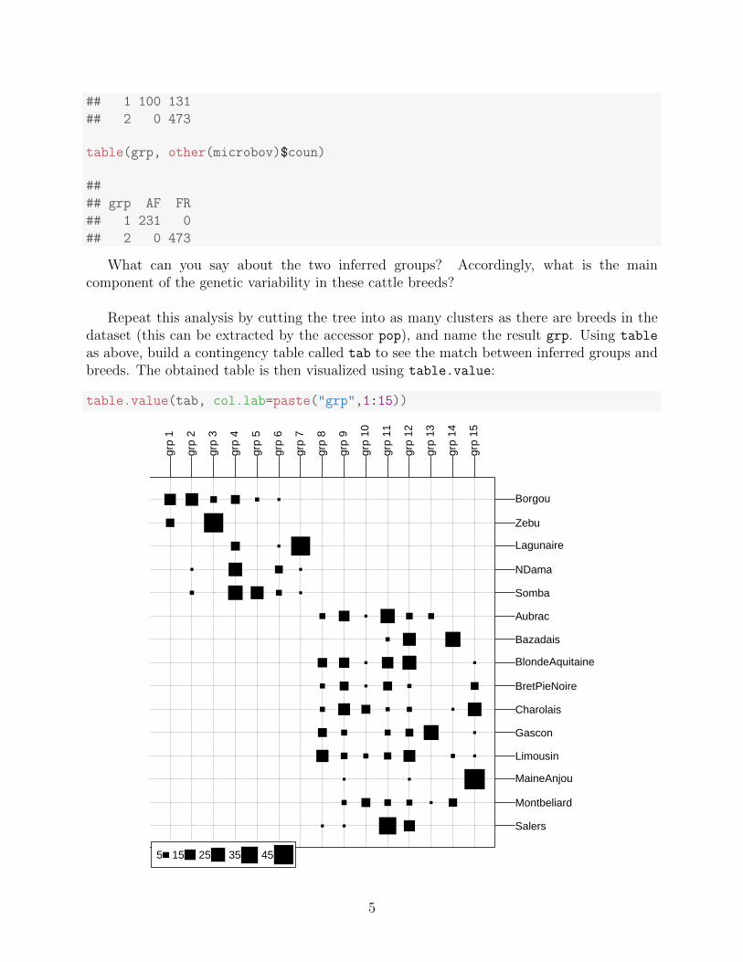
## 1 100 131

## 2 0 473

table(grp, other(microbov)$coun)

##

## grp AF FR

## 1 231 0

## 2 0 473

What can you say about the two inferred groups? Accordingly, what is the maincomponent of the genetic variability in these cattle breeds?

Repeat this analysis by cutting the tree into as many clusters as there are breeds in thedataset (this can be extracted by the accessor pop), and name the result grp. Using table

as above, build a contingency table called tab to see the match between inferred groups andbreeds. The obtained table is then visualized using table.value:

table.value(tab, col.lab=paste("grp",1:15))

Borgou

Zebu

Lagunaire

NDama

Somba

Aubrac

Bazadais

BlondeAquitaine

BretPieNoire

Charolais

Gascon

Limousin

MaineAnjou

Montbeliard

Salers

grp

1

grp

2

grp

3

grp

4

grp

5

grp

6

grp

7

grp

8

grp

9

grp

10

grp

11

grp

12

grp

13

grp

14

grp

15

5 15 25 35 45

5

Can some groups be identified as species or breeds? Do some species look more admixedthan others?

1.2 K-means

K-means is another, non-hierarchical approach for defining genetic clusters. While basicK-means is implemented in the function kmeans, the function find.clusters provides acomputer-efficient implementation which first reduces the dimensionality of the data (usingPCA), and optionally allows for choosing the optimal number of clusters using BayesianInformation Criteria (BIC). Use find.clusters to obtain 15 groups and store the result inan object called grp. If unsure how to use the function, remember to check the help page(?find.clusters).

How many clusters would you have selected relying on the BIC?

Using table.value as before, visualize the correspondence between inferred groups andactual breeds:

table.value(table(pop(microbov), grp$grp), col.lab=paste("grp", 1:15))

Borgou

Zebu

Lagunaire

NDama

Somba

Aubrac

Bazadais

BlondeAquitaine

BretPieNoire

Charolais

Gascon

Limousin

MaineAnjou

Montbeliard

Salers

grp

1

grp

2

grp

3

grp

4

grp

5

grp

6

grp

7

grp

8

grp

9

grp

10

grp

11

grp

12

grp

13

grp

14

grp

15

5 15 25 35 45 55

6

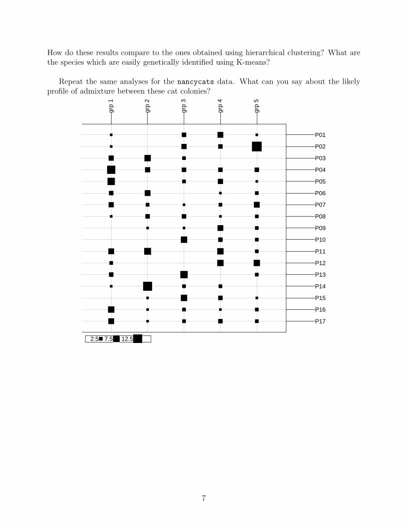
How do these results compare to the ones obtained using hierarchical clustering? What arethe species which are easily genetically identified using K-means?

Repeat the same analyses for the nancycats data. What can you say about the likelyprofile of admixture between these cat colonies?

P01

P02

P03

P04

P05

P06

P07

P08

P09

P10

P11

P12

P13

P14

P15

P16

P17

grp

1

grp

2

grp

3

grp

4

grp

5

2.5 7.5 12.5

7

2 Describing group diversity: Maripaulis nonsensicus

populations

2.1 Maripaulis nonsensicus: first contact

The first study of group diversity focuses on Maripaulis nonsensicus, a diploid plant well-known for having a number of cryptic sub-species. A total of 600 individual plants have beensampled in the Scotish countryside and genotyped for 30 microsatellite markers. We firstload the dataset, which has already been converted to a genind object:

load(url("http://adegenet.r-forge.r-project.org/files/PRstats/Mnonsensicus1.RData"),

verbose=TRUE)

## Loading objects:

## Mnonsensicus1

Mnonsensicus1

## /// GENIND OBJECT /////////

##

## // 600 individuals; 30 loci; 140 alleles; size: 401.6 Kb

##

## // Basic content

## @tab: 600 x 140 matrix of allele counts

## @loc.n.all: number of alleles per locus (range: 2-8)

## @loc.fac: locus factor for the 140 columns of @tab

## @all.names: list of allele names for each locus

## @ploidy: ploidy of each individual (range: 2-2)

## @type: codom

## @call: .local(.Object = .Object, tab = ..1)

##

## // Optional content

## - empty -

The main goal of the study is to assess whether the sampled plants all belong tothe same panmictic population, or whether sub-populations can be identified. First, use

8

find.clusters to identify the number and nature of potential genetic clusters, and storethe result in an object called grp1.

How many clusters do you identify? Are these dependent on how many principalcomponents (PCs) you retain? What are the respective group sizes?

We want to assess the relationships between these groups using DAPC. Using the followingcommand, perform the DAPC and store the results in a new object called dapc1:

dapc1 <- dapc(Mnonsensicus1, pop=grp1$grp, scale=FALSE)

Use the function scatter to visualize the results. This function has many options, whichare documented in ?scatter.dapc. Your graphic should roughly ressemble:

scatter(dapc1, col=funky(6), scree.pca=TRUE)

1

2

3

4 5

6

1

2

3

4 5

6

DA eigenvaluesPCA eigenvalues

The function scatter plots by default the first two discriminant functions. Tryvisualizing other possibly relevant axes. What can you tell about the structure of thispopulation?

9

It may be useful to compare these results to an alternative approach. Computethe Euclidian distances (function dist) between the matrix of allele frequenciestab(Mnonsensicus1, freq=TRUE), and use them to build a Neighbour-Joining tree(implemented in the ape package). Examine the tree. This should look like:

Mnonsensicus tree 1

●

●

●

●

● ●

●●

●

●

●

●

●

●

●

●

●

●

●

●

●

●●

● ●

●

●

●

●

●

●

●

●

●

●

●

●

●

●●

●

●

●

●

●

●

●

●

● ●

●

●

●

●

●

●

●

●

●

●

●

●

●

●

●

●

●

●

●

●

●

●

●

●

●●

●

●

●

●

●

●

●

●

●

●

●

●●

●

●

●

●

●

●

●

●

●●

●

●

●

●

●

●

●●

●

●

●

●

●

● ●

●

●

●

●●

●

● ●

●

●

●

●

●

●

●●

●

●

●

●

●

●

●

●

●

●

●

●

●

●

●●

●

●

●

●●

●

●●

●●

●●

●

●

●

●

●

●

● ●

●

●

●●

●●

●

●

●

●

●

●

●

●

●●

●●

●●

●

●

●●

●●

●

●

●

●●

●

●●

●

●

● ●●

●

●

●

●

●

●

●

●●

●

●

●

●

●

●

●

●●

●

●

●

●

●

●

●

●

●

●

●

●

●

●

●

●

●

●

●

●

●

●

●

●

●

●

●

●

●●

●

●

●

●

●

●

●

●

●

●

●

●

●

●

●

●

●

●

●

●

●

●

●

●

●

●

●

●

●

●

●

●

●

●

●

●●

●

●

●

●

●

●

●

●● ●

●

●

●

●

●

●

●●

●

●

●

●

●

●●

●

●

●

●● ●

●

●

●

●

●

●●

●

●

●

●

●

●

●●

●

●● ●

●

●

●●

●●

●

●

●●

●

●

●

●

●

●

●●

● ●●●

●

●

●

●

● ●

●

●●

●

●

●

●

●

●

●

●●●

●

●

●

●

●

●

●

●

●

●

●

●

●

●

● ●●

●

●

●

●

●

●

●

●

●●

●

●

●

●

●

●

●

●

●

●●●

●

●●

●

●●

●

●

●

●

●

●●

●

●

●

●

●

●●

●●

● ●

●

●

●

●●

●

●

●

●

●

●

●

●

●●

●

●

●

●

●

●

●

●

●

●

●

●

●

●

●

●●

●●

● ●

●

●

●

●

●

●

●

●

●

●

●

●

●

●

●

● ●

●●

●

●●

●●

●

●●

●

●

●

●

●●

●

●

●

●

●●

●

●

●

●

●

●

●

●

●

●

●

● ●

●

●

●

●●

●

●

●

●●

●

●

●

●

●

●

●

●

●

●

●●

●

●

●

●

●

●

●

●●

●

●

●

●

●

●

●

●

●

●

●

●

●

●

●

●

●

●●

●

●

● ●●

●

●

●

●

●●

●

●

●●

●●

●

What are your conclusions?

2.2 Maripaulis nonsensicus: the return

After the initial study of E. nonsensicus populations, the sampling area has been extendedand new populations have been discovered. A new sample of 450 plants has been characterizedfor the same 30 microsatellite markers. Your task is to conduct the same kind of analysis,and assess the genetic makeup of the new population.

load(url("http://adegenet.r-forge.r-project.org/files/PRstats/Mnonsensicus2.RData"),

verbose=TRUE)

## Loading objects:

## Mnonsensicus2

10

Mnonsensicus2


##


##

## // Basic content






## @type: codom

## @call: .local(.Object = .Object, tab = ..1)

##


## - empty -

Again, use find.clusters to identify the number and nature of potential geneticclusters, and store the result in an object called grp2. How many clusters would you retain?How do the results compare to the previous study?

Try assessing the relationships between these clusters using dapc. If results seem unstablefrom one run to another, try increasing the number of starting points used in the K-meansalgorithm (argument n.start).

Use the function scatter to visualize the results. Specify that you want the minimumspanning tree added to link together the closest populations. With a bit of customisation(see ?scatter.dapc), your graphic should ressemble:

11

123456789101112

DA eigenvaluesPCA eigenvalues

What can you say about the structure of this population? Assuming this structure isessentially spatial, what kind of spatial processes could have generated the observed patterns?

12

3 Describing group diversity: cattle breed

discrimination and alien abductions

3.1 Choosing how many components to retain

DAPC relies on a ‘simplification’ of the data using a PCA as a prior step to DiscriminantAnalysis. As always in multivariate analysis, the choice of the number of PCs to retain isnot trivial. Let us illustrate the impact of this choice on the results using the microbov

dataset (704 cattles of 15 breeds typed for 30 microsatellite markers). We first examine the% of successful reassignment (i.e., quality of discrimination) for different numbers of retainedPCs. First, retaining only 10 PCs during the dimension-reduction step, and all discriminantfunctions:

data(microbov)

microbov


##

## // 704 individuals; 30 loci; 373 alleles; size: 1.1 Mb

##

## // Basic content






## @type: codom

## @call: genind(tab = truenames(microbov)$tab, pop = truenames(microbov)$pop)

##


## @pop: population of each individual (group size range: 30-61)

## @other: a list containing: coun breed spe

temp <- summary(dapc(microbov, n.da=100, n.pca=10))$assign.per.pop*100

par(mar=c(4.5,7.5,1,1))

barplot(temp, xlab="% of reassignment to actual breed",

horiz=TRUE, las=1)

13

Borgou

Zebu

Lagunaire

NDama

Somba

Aubrac

Bazadais

BlondeAquitaine

BretPieNoire

Charolais

Gascon

Limousin

MaineAnjou

Montbeliard

Salers

% of reassignment to actual breed

0 20 40 60 80 100

We can see that some breeds are well discriminated while others are mostly overlooked bythe analysis. This is because too much genetic information is lost when retaining only 10PCs. We repeat the analysis, this time keeping 300 PCs:

temp <- summary(dapc(microbov, n.da=100, n.pca=300))$assign.per.pop*100

par(mar=c(4.5,7.5,1,1))

barplot(temp, xlab="% of reassignment to actual breed", horiz=TRUE, las=1)

14

Borgou

Zebu

Lagunaire

NDama

Somba

Aubrac

Bazadais

BlondeAquitaine

BretPieNoire

Charolais

Gascon

Limousin

MaineAnjou

Montbeliard

Salers


0 20 40 60 80 100

We now obtain almost 100% discrimination for all groups. Is this result satisfying? Let ustry again, this time using randomised groups in the analysis:

x <- microbov

pop(x) <- sample(pop(x))

temp <- summary(dapc(x, n.da=100, n.pca=300))$assign.per.pop*100

par(mar=c(4.5,7.5,1,1))

barplot(temp, xlab="% of reassignment to actual breed", horiz=TRUE, las=1)

15

BretPieNoire

Salers

Lagunaire

Somba

Limousin

BlondeAquitaine

Borgou

Aubrac

Montbeliard

NDama

Gascon

Charolais

MaineAnjou

Zebu

Bazadais


0 20 40 60 80

Groups have been randomised, and yet we still obtain very good discrimination. Why is this?

In attempting to summarise high-dimensional data in a small number of meaningfuldiscriminant functions, DAPC must manage a trade-off. If too few PCs (with respectto the number of individuals) are retained, useful information will be excluded from theanalysis, and the resulting model will not be informative enough to accurately discriminatebetween groups. By contrast, if too many PCs are retained, the discriminant functions willbe over-fitted and capable of discriminating any clusters. In this case, the discriminantfunctions will be completely tailored to the dataset, and loose any ability to generalize tonew or unseen data.

3.2 Using cross-validation

As discussed above, choosing the ‘right’ number of PCs in DAPC is not a trivial task. As themain goal could be formulated as finding the number of PCs which ‘maximizes the probabilityof assigning new individuals to their actual group’, one natural approach to address this issueis cross-validation. Cross-validation (function xvalDapc) provides an objective optimisationprocedure for identifying the ’goldilocks point’ in the trade-off between retaining too few

16

and too many PCs in the model. In cross-validation, the data is divided into two sets: atraining set (typically comprising 90% of the data) and a validation set (which contains theremainder (by default, 10%) of the data). With xvalDapc, the validation set is selectedby stratified random sampling: this ensures that at least one member of each group orpopulation in the original data is represented in both training and validation sets.

DAPC is carried out on the training set with variable numbers of PCs retained, and thedegree to which the analysis is able to accurately predict the group membership of excludedindividuals (those in the validation set) is used to identify the optimal number of PCs toretain. At each level of PC retention, the sampling and DAPC procedures are repeatedn.rep times. Let us apply this method to the microbov dataset:

mat <- tab(microbov, NA.method="mean")

grp <- pop(microbov)

xval <- xvalDapc(mat, grp, n.pca.max=200, training.set=0.9,

result="groupMean", scale=FALSE, n.rep=10,

n.pca=c(5,10,seq(25,by=25,to=200)),

xval.plot = TRUE)

0 50 100 150 200

0.0

0.2

0.4

0.6

0.8

1.0

DAPC Cross−Validation

Number of PCA axes retained

Pro

port

ion

of s

ucce

ssfu

l out

com

e pr

edic

tion

When xval.plot is TRUE, a scatterplot of the DAPC cross-validation is generated.The number of PCs retained in each DAPC varies along the x-axis, and the proportion of

17

successful outcome prediction varies along the y-axis. Individual replicates appear as points,and the density of those points in different regions of the plot is displayed in blue.

names(xval)

## [1] "Cross-Validation Results"

## [2] "Median and Confidence Interval for Random Chance"

## [3] "Mean Successful Assignment by Number of PCs of PCA"

## [4] "Number of PCs Achieving Highest Mean Success"

## [5] "Root Mean Squared Error by Number of PCs of PCA"

## [6] "Number of PCs Achieving Lowest MSE"

## [7] "DAPC"

xval[2:6]

## $`Median and Confidence Interval for Random Chance`

## 2.5% 50% 97.5%

## 0.05053353 0.06667563 0.08387159

##

## $`Mean Successful Assignment by Number of PCs of PCA`

## 5 10 25 50 75 100 125

## 0.5724444 0.6997778 0.8271111 0.8571111 0.8873333 0.8968889 0.8957778

## 150 175 200

## 0.8948889 0.8893333 0.8706667

##

## $`Number of PCs Achieving Highest Mean Success`

## [1] "100"

##

## $`Root Mean Squared Error by Number of PCs of PCA`

## 5 10 25 50 75 100 125

## 0.4307238 0.3027960 0.1767275 0.1522133 0.1200350 0.1059606 0.1079163

## 150 175 200

## 0.1126011 0.1136553 0.1334925

##

## $`Number of PCs Achieving Lowest MSE`

## [1] "100"

The ideal result of this cross-validation procedure would be a bell-shaped relationship,indicating the optimal number of PCs to retain. Here, most solutions beyond 75 PCs seemequivalent. Make your own DAPC of microbov choosing your preferred number of PCs andstore the result in dapc.bov.

18

3.3 Alien abductions

After your analysis of the optimal discrimination of cattle breeds, you are contactedby some governmental officers to investigate the possible origin of blood samples comingfrom cattles allegedly abducted by aliens. Blood samples have been found in twodifferent saucepans. The resulting datasets are respectively named unknown1 and unknown2

(governmental officers notoriously lack originality). The files are available as RData from thefollowing URLs:

load(url("http://adegenet.r-forge.r-project.org/files/PRstats/unknown1.RData"),

verbose=TRUE)

## Loading objects:

## unknown1

unknown1


##


##

## // Basic content






## @type: codom

## @call: NULL

##


## - empty -

load(url("http://adegenet.r-forge.r-project.org/files/PRstats/unknown2.RData"),

verbose=TRUE)

## Loading objects:

## unknown2

19

unknown2


##


##

## // Basic content






## @type: codom

## @call: NULL

##


## - empty -

As seen before, DAPC can be used to predict group memberships of individuals based ontheir scores on the discriminant functions. One advantage of this approach is that the samecan be done with new individuals, provided the new data have exactly the same variablesas the ones used in the analysis. First, let us check that the loci and alleles in the two newdatasets (unknown1 and unknown2) are identical to the microbov data:

## look at the loci

locNames(microbov)

## [1] "INRA63" "INRA5" "ETH225" "ILSTS5" "HEL5" "HEL1" "INRA35"

## [8] "ETH152" "INRA23" "ETH10" "HEL9" "CSSM66" "INRA32" "ETH3"

## [15] "BM2113" "BM1824" "HEL13" "INRA37" "BM1818" "ILSTS6" "MM12"

## [22] "CSRM60" "ETH185" "HAUT24" "HAUT27" "TGLA227" "TGLA126" "TGLA122"

## [29] "TGLA53" "SPS115"

locNames(unknown1)

## [1] "BM1818" "BM1824" "BM2113" "CSRM60" "CSSM66" "ETH10" "ETH152"

## [8] "ETH185" "ETH225" "ETH3" "HAUT24" "HAUT27" "HEL1" "HEL13"

## [15] "HEL5" "HEL9" "ILSTS5" "ILSTS6" "INRA23" "INRA32" "INRA35"

## [22] "INRA37" "INRA5" "INRA63" "MM12" "SPS115" "TGLA122" "TGLA126"

## [29] "TGLA227" "TGLA53"

locNames(unknown2)

## [1] "BM1818" "BM1824" "BM2113" "CSRM60" "CSSM66" "ETH10" "ETH152"

## [8] "ETH185" "ETH225" "ETH3" "HAUT24" "HAUT27" "HEL1" "HEL13"

20

## [15] "HEL5" "HEL9" "ILSTS5" "ILSTS6" "INRA23" "INRA32" "INRA35"

## [22] "INRA37" "INRA5" "INRA63" "MM12" "SPS115" "TGLA122" "TGLA126"

## [29] "TGLA227" "TGLA53"

identical(sort(locNames(microbov)), sort(locNames(unknown1)))

## [1] TRUE

identical(sort(locNames(microbov)), sort(locNames(unknown2)))

## [1] TRUE

The same loci have been sequenced, but they are in a different order. Also, nothingguarantees the same alleles are present in all datasets, or in the same order. We use repool

to work around this problem:

## repool all datasets

bov <- microbov

pop(bov) <- rep("bov",nInd(microbov))

pop(unknown1) <- rep("unknown1",nInd(unknown1))

pop(unknown2) <- rep("unknown2",nInd(unknown2))

temp <- seppop(repool(bov, unknown1, unknown2))

## extract data

names(temp)

## [1] "bov" "unknown1" "unknown2"

bov <- temp[[1]]

unknown1 <- temp[[2]]

unknown2 <- temp[[3]]

## restore populations in bov

pop(bov) <- pop(microbov)

## check loci again

identical(locNames(bov, withAlleles=TRUE), locNames(unknown1, withAlleles=TRUE))

## [1] TRUE

identical(locNames(bov, withAlleles=TRUE), locNames(unknown2, withAlleles=TRUE))

## [1] TRUE

We also need to repeat the previous DAPC, as variables have now changed (they havebeen reordered):

21

dapc.bov <- dapc(bov,n.pca=75,n.da=14)

Look at the documentation of predict.dapc, and use the function to predict where theabducted cattles came from.

If the output of predict are called pred1 and pred2, you can visualise the predictedgroup memberships using:

par(xpd=TRUE, mar=c(8,4,8,3))

barplot(t(100*round(pred1$posterior,2)), col=funky(15),

ylab="% assignment",las=3)

legend("top", fill=funky(15),

legend=levels(pop(microbov)),

ncol=4,inset=c(0,-.3))

unkn

own0

1

unkn

own0

2

unkn

own0

3

unkn

own0

4

unkn

own0

5

unkn

own0

6

unkn

own0

7

unkn

own0

8

unkn

own0

9

unkn

own1

0

% a

ssig

nmen

t

020

4060

8010

0

BorgouZebuLagunaireNDama

SombaAubracBazadaisBlondeAquitaine

BretPieNoireCharolaisGasconLimousin

MaineAnjouMontbeliardSalers

par(xpd=TRUE, mar=c(8,4,8,3))

barplot(t(100*round(pred2$posterior,2)), col=funky(15),

ylab="% assignment", las=3)

22

legend("top", fill=funky(15),

legend=levels(pop(microbov)),

ncol=4,inset=c(0,-.3))

unkn

own1

unkn

own2

unkn

own3

unkn

own4

unkn

own5

unkn

own1

1

unkn

own2

1

unkn

own3

1

unkn

own4

1

unkn

own5

1

unkn

own0

11

unkn

own0

21

unkn

own0

31

unkn

own0

41

unkn

own0

51

unkn

own0

61

unkn

own0

71

unkn

own0

81

unkn

own0

91

unkn

own1

01

% a

ssig

nmen

t

020

4060

8010

0

BorgouZebuLagunaireNDama

SombaAubracBazadaisBlondeAquitaine

BretPieNoireCharolaisGasconLimousin

MaineAnjouMontbeliardSalers

What are your conlcusions?

23

4 To go further

DAPC is more extensively covered in a dedicated tutorial which you can access from theadegenet website:http://adegenet.r-forge.r-project.org/

or by typing:

adegenetTutorial("dapc")

The paper presenting the method is in open access online:http://www.biomedcentral.com/1471-2156/11/94

Lastly, as of version 1.4-0 of adegenet, a web interface for DAPC can be started fromR using:

adegenetServer("DAPC")

24

http://adegenet.r-forge.r-project.org/

http://www.biomedcentral.com/1471-2156/11/94

multivariate analysis of genetic data: exploring group

Documents