multivariate features for multi-class brain computer ... · multivariate features for multi-class...
TRANSCRIPT
Multivariate Features for Multi-class
Brain Computer Interface Systems
A thesis submitted for the degree
of PhD in Information Sciences and Engineering of
the University of Canberra
Tuan Than Anh Hoang
May 18, 2014

Summary of Thesis
Brain-Computer Interface (BCI) is an emerging research field attracting a lot of research
attention in an effort to build up a new way for communicating between computers and
humans using brain signals. However, the performance of multi-class BCI systems is still
not high enough. This research targets the feature extraction phase for Multi-Class BCI
systems based on motor imagery. By analyzing the properties of covariance matrices and
the nature of brain signals through experiments, the research proposes two new methods
of feature extraction in BCI systems. The first method is called Approximation-based
Common Principal Components (ACPC) analysis. This method aims at finding a common
subspace from original subspaces which contain information of classes. Compared with the
current state-of-the-art methods based on Common Spatial Patterns (CSP), this method
directly deals with multi-class problems instead of converting multi-class problems into
many 2-class problems. The second method is based on Aggregate Models. Its main idea
comes from a highly challenging problem of large inter-subject and inter-session variability
in BCI experiments. Exploiting these characteristics, this method can be used not only in
Subject-Dependent Multi-Class BCI systems but also in Subject-Independent Multi-Class
BCI ones. A combination of the proposed methods leads to a new method called Segmented
Spatial Filters (SSF). The SSF method can not only improve spatial resolution of brain
signals but also efficiently deal with inter-subject and inter-session variability in multi-class
BCI systems.
Experiments were conducted on the Dataset 2a of the BCI Competition IV which is
a well known dataset for multi-class BCI systems. Experimental results show that the
proposed ACPC and Aggregate Model methods are superior to current state-of-the-art
feature extraction methods that are based on CSP. The later model can also be applied
in Subject-Independent Multi-Class BCI systems in a natural way with better accuracy
compared with other related methods.
iii

Contributions of Thesis
Contributions of the thesis has three folds. The first contribution is a new method called
Approximation-based Common Principal Components (ACPC) analysis. This method can
directly deal with multi-class BCI problems instead of converting a multi-class problem into
many 2-class problems. The experiments of this method on a standard BCI dataset showed
that it can achieve better classification accuracy than the 2-class-based methods.
The second contribution is a new method based on Aggregate Models. This method
exploits the problem of large inter-subject and inter-session variability in BCI experiments.
The conducted experiments showed that Aggregate Models can be used not only in Subject-
Dependent Multi-Class BCI systems but also in Subject-Independent Multi-Class BCI sys-
tems. A successful application of Subject-Independent Multi-Class BCI systems can reduce
learning time of new and inexperienced users of BCI systems.
The last contribution is based on a combination of the two proposed methods. It is
named Segmented Spatial Filters (SSF). The SSF method can not only improve spatial
resolution of brain signals but also efficiently deal with inter-subject and inter-session vari-
ability in multi-class BCI systems.
v

Acknowledgements
First and foremost, I would like to thank my supervisor A/Prof. Dat Tran. He
has enormously supported my study at the University of Canberra. I appreciate all
his contributions of time, ideas, advice, and funding supports to make my Ph.D.
experience productive and stimulating. I would also like to thank my co-supervisors,
Prof. Xu Huang and Prof. Dharmendra Sharma for their time, support and ideas on
my research.
In regard to the fNIRS experiments, I would love to thank Prof. Vo Van Toi and
Dr. Truong Quang Dang Khoa at Laboratory of Biomedical Engineering Department
of International University, Viet Nam. Without their help, I could not successfully
conduct the experiments.
I gratefully acknowledge the generous funding support sources that allow me to
pursue this Ph.D. research. I was funded by the International Postgraduate Research
Scholarships scheme which is co-sponsored by the Australian government and the
University of Canberra, and by the W J Weeden Top Up Scholarship.
My time at the University of Canberra was made enjoyable due to many friends
whom I met and worked with here. My sincere thanks is to A/Prof Girija Chetty for
her kind invitation for being her assistant lecture. I would also love to thank the staff
members, especially to Serena Chong, Kylie Reece, and Jason Weber for their quick
and helpful response in administration work. Thanks to the research students of the
Faculty of EsTEM for their useful discussions and seminars. A very warm thank to
Mr. Hanh Huynh for his advices, encouragement and coffee. It is my pleasure to meet
you here, my uncle. A grateful thank to my brothers and friends Trung Le, Amanda
Jones, Phuoc Nguyen, and Dat Huynh.
I would like to express my appreciation to Beth Barber from the Faculty of Arts
and Design, University of Canberra for her excellent editing. Her editing skills helped
ix

x
me see the blind spots of the thesis and suggested better options for expressing my
ideas.
Lastly, I would like to thank my family for all their love and support. To my
parents who raised me up with their endless love, support and encouragement. To
my brothers and sister who always support me in all my pursuits. And most of all to
my loving and supportive wife Hannah and my little boy Khoa whose happiness has
always been the biggest motivation in my life.

Contents
Summary of Thesis iii
Contributions of Thesis v
Acknowledgements ix
Abbreviation xxiii
List of Symbols xxvii
1 Introduction 1
1.1 Research context . . . . . . . . . . . . . . . . . . . . . . . . . . . . . 1
1.1.1 Data acquisition . . . . . . . . . . . . . . . . . . . . . . . . . . 2
1.1.2 Pre-processing . . . . . . . . . . . . . . . . . . . . . . . . . . . 2
1.1.3 Feature extraction . . . . . . . . . . . . . . . . . . . . . . . . 3
1.1.4 Classification . . . . . . . . . . . . . . . . . . . . . . . . . . . 3
1.1.5 Application interface . . . . . . . . . . . . . . . . . . . . . . . 3
1.1.6 Feedback . . . . . . . . . . . . . . . . . . . . . . . . . . . . . . 4
1.2 Brief introduction to EEG-based BCI systems . . . . . . . . . . . . . 4
1.3 Problem statement . . . . . . . . . . . . . . . . . . . . . . . . . . . . 8
1.4 Targets of the research and brief of methodology . . . . . . . . . . . . 9
1.4.1 Targets of the research . . . . . . . . . . . . . . . . . . . . . . 9
1.4.2 Brief of Methodology . . . . . . . . . . . . . . . . . . . . . . . 10
1.5 The thesis outline . . . . . . . . . . . . . . . . . . . . . . . . . . . . . 10
xi
CONTENTS xii
2 Literature Review 13
2.1 Brain-Computer Interface . . . . . . . . . . . . . . . . . . . . . . . . 13
2.1.1 Data acquisition in BCI . . . . . . . . . . . . . . . . . . . . . 14
2.1.2 Types of control signal in BCI . . . . . . . . . . . . . . . . . . 16
2.1.3 Pre-processing methods in BCI . . . . . . . . . . . . . . . . . 18
2.1.4 Classifiers in BCI . . . . . . . . . . . . . . . . . . . . . . . . . 19
2.1.5 Existing BCI Applications and Systems . . . . . . . . . . . . . 21
2.2 Feature extraction in BCI systems . . . . . . . . . . . . . . . . . . . . 22
2.2.1 Feature extraction in general BCI systems . . . . . . . . . . . 22
Single-channel feature extraction methods . . . . . . . . . . . 22
Multi-channel feature extraction methods . . . . . . . . . . . . 27
Common Spatial Patterns . . . . . . . . . . . . . . . . . . . . 31
2.2.2 Feature extraction in Multi-class BCI systems . . . . . . . . . 39
2.2.3 Feature extraction in subject-dependent and subject-independent
BCI systems . . . . . . . . . . . . . . . . . . . . . . . . . . . . 42
2.3 Activation and delay issue in BCI experiments . . . . . . . . . . . . . 43
2.4 Functional Near Infrared Spectroscopy . . . . . . . . . . . . . . . . . 44
2.5 Aggregate model related methods . . . . . . . . . . . . . . . . . . . . 45
2.5.1 Adaptive boosting method . . . . . . . . . . . . . . . . . . . . 45
2.5.2 Decision tree learning . . . . . . . . . . . . . . . . . . . . . . . 47
3 Multi-class Brain-Computer Interface Systems and Baseline Meth-
ods 49
3.1 Formulation of Brain-Computer Interface . . . . . . . . . . . . . . . . 49
3.2 Common Spatial Patterns (CSP) analysis in 2-class BCI systems . . . 50
3.2.1 Two-class CSP . . . . . . . . . . . . . . . . . . . . . . . . . . 51
3.2.2 CSP-based feature extraction in BCI systems . . . . . . . . . 51
3.3 CSP-based extensions for multi-class BCI systems . . . . . . . . . . 52
3.3.1 One-versus-the-Rest CSP . . . . . . . . . . . . . . . . . . . . . 52
3.3.2 Pair-wise CSP . . . . . . . . . . . . . . . . . . . . . . . . . . . 53
3.3.3 Union-based Common Principal Components . . . . . . . . . . 53
3.4 Time Domain Parameters . . . . . . . . . . . . . . . . . . . . . . . . 53
CONTENTS xiii
3.4.1 Relationship between Time Domain Parameters and other spec-
tral power based features . . . . . . . . . . . . . . . . . . . . . 54
4 Common Principal Component Analysis for Multi-Class Brain-Computer
Interface Systems 57
4.1 Jacobian-based ACPC . . . . . . . . . . . . . . . . . . . . . . . . . . 58
4.1.1 Jacobian-based algorithm for finding Common Principal Com-
ponents . . . . . . . . . . . . . . . . . . . . . . . . . . . . . . 58
4.1.2 Ranking Common Principal Components and the relationship
between Common Principal Components and 2-class Common
Spatial Patterns . . . . . . . . . . . . . . . . . . . . . . . . . . 60
4.1.3 Feature extraction based on Jacobian-based Common Principal
Components . . . . . . . . . . . . . . . . . . . . . . . . . . . . 61
4.2 2PCA Approximation-based Common Principal Components . . . . . 63
4.2.1 2PCA Approximation-based Common Principal Components . 63
4.2.2 Feature extraction based on 2PCA Approximation-based Com-
mon Principal Component analysis . . . . . . . . . . . . . . . 66
5 Experiments with Approximation-based Common Principal Compo-
nent Analysis 69
5.1 Dataset used in experiments . . . . . . . . . . . . . . . . . . . . . . . 69
5.2 Experiment methods and validations . . . . . . . . . . . . . . . . . . 72
5.3 Experimental results . . . . . . . . . . . . . . . . . . . . . . . . . . . 73
5.3.1 Comparison with CSP 1vsN and CSP pairs methods . . . . 74
5.3.2 Comparison with Time Domain Parameters method . . . . . . 75
5.4 Discussion . . . . . . . . . . . . . . . . . . . . . . . . . . . . . . . . . 78
5.4.1 Visualization of Approximation-based Common Principal Com-
ponents . . . . . . . . . . . . . . . . . . . . . . . . . . . . . . 78
5.4.2 Effect of the number of selected common principal components
on classification accuracy of 2PCA ACPC . . . . . . . . . . . 79
5.4.3 Effect of the number of selected common principal components
on classification accuracy of Jacobi ACPC . . . . . . . . . . . 82
CONTENTS xiv
5.4.4 Comparison with participants of BCI Competition IV on Dataset
2a . . . . . . . . . . . . . . . . . . . . . . . . . . . . . . . . . 83
6 General Aggregate Models for Motor Imagery-Based BCI Systems 87
6.1 Activation and delay issue in BCI experiments . . . . . . . . . . . . . 87
6.2 Analysis on activation and delay issue using fNIRS . . . . . . . . . . 88
6.2.1 Subjects . . . . . . . . . . . . . . . . . . . . . . . . . . . . . . 88
6.2.2 Experimental procedure . . . . . . . . . . . . . . . . . . . . . 89
6.2.3 Data acquisition . . . . . . . . . . . . . . . . . . . . . . . . . . 89
6.2.4 Results on activation and delay issue experiment . . . . . . . . 91
6.3 A general aggregate model at score level for BCI systems . . . . . . . 92
6.4 A general aggregate model at feature level for BCI systems . . . . . . 94
6.5 Segmented Spatial Filters for MBCI systems . . . . . . . . . . . . . . 96
7 Experiments with Aggregate Models 99
7.1 Dataset used in experiments . . . . . . . . . . . . . . . . . . . . . . . 99
7.2 Experiment methods and validations . . . . . . . . . . . . . . . . . . 100
7.3 Experimental results . . . . . . . . . . . . . . . . . . . . . . . . . . . 102
7.3.1 Aggregate models in subject-dependent multi-class BCI systems 102
7.3.2 Aggregate models in subject-independent multi-class BCI systems107
7.4 Discussion . . . . . . . . . . . . . . . . . . . . . . . . . . . . . . . . . 113
7.4.1 Aggregate models in 2-class subject-dependent multi-class BCI
systems . . . . . . . . . . . . . . . . . . . . . . . . . . . . . . 113
7.4.2 SD-MBCI systems versus SI-MBC systems . . . . . . . . . . . 116
7.4.3 Aggregate models with TDP features . . . . . . . . . . . . . . 116
7.4.4 Fixed segmentation and dynamic segmentation in aggregate
models at feature level . . . . . . . . . . . . . . . . . . . . . . 121
7.4.5 Toward online multi-class BCI systems . . . . . . . . . . . . . 124
8 Conclusions and Future Research 129
8.1 Conclusions . . . . . . . . . . . . . . . . . . . . . . . . . . . . . . . . 129
8.2 Future research . . . . . . . . . . . . . . . . . . . . . . . . . . . . . . 134
Appendices 135

CONTENTS xv
Publications 137
Bibliography 139

List of Figures
1.1 A typical BCI scheme. . . . . . . . . . . . . . . . . . . . . . . . . . . 1
1.2 Conventional 10-20 EEG electrode positions for 21 electrodes . . . . . 5
2.1 A simple brain structure (from www.wikipedia.org). . . . . . . . . . . 17
5.1 Timing scheme used in dataset 2a of the BCI Competition IV . . . . 70
5.2 The electrode positions used in dataset 2a of the BCI Competition IV 71
5.3 Comparison between CSP 1vsN and CSP pairs methods. . . . . . . 75
5.4 Ranking of ACPC and CSP methods based on classification accuracy
average over all nine subjects. . . . . . . . . . . . . . . . . . . . . . . 76
5.5 Comparison between Mobility and Complexity features. . . . . . . . 77
5.6 Ranking of ACPC methods and TDP features based on classification
accuracy average over all nine subjects. . . . . . . . . . . . . . . . . . 77
5.7 Visualization of three sample common principal components . . . . . 78
5.8 The effect of the number of selected components of 2PCA ACPC . . 80
5.9 The effect of the number of selected components of 2PCA ACPC com-
pared with CSP -based methods . . . . . . . . . . . . . . . . . . . . . 81
5.10 The effect of the number of selected components of 2PCA ACPC com-
pared with TDP . . . . . . . . . . . . . . . . . . . . . . . . . . . . . 81
5.11 The effect of the number of selected components of Jacobi ACPC . . 82
5.12 The effect of the number of selected components of Jacobi ACPC com-
pared with CSP -based methods . . . . . . . . . . . . . . . . . . . . . 83
5.13 The effect of the number of selected components of Jacobi ACPC com-
pared with TDP . . . . . . . . . . . . . . . . . . . . . . . . . . . . . 84
xvii

LIST OF FIGURES xviii
5.14 Comparison of classification accuracy between ACPC and methods of
the participants on average . . . . . . . . . . . . . . . . . . . . . . . . 86
6.1 Protocols were used in fNIRS experiments . . . . . . . . . . . . . . . 90
6.2 Optode positions used in the fNIRS experiments . . . . . . . . . . . . 91
6.3 A general aggregate model at score level for BCI systems. . . . . . . . 93
6.4 A general aggregate model at feature level for BCI systems . . . . . . 94
7.1 Comparison between CSP 1vsN and its aggregate models. . . . . . . 103
7.2 Comparison between CSP pairs and its aggregate models. . . . . . . 104
7.3 Comparison between 2PCA ACPC and its aggregate models. . . . . 104
7.4 Comparison between CSP 1vsN and its framed version . . . . . . . . 106
7.5 Comparison between CSP pairs and its framed version . . . . . . . . 106
7.6 Comparison between 2PCA ACPC and its framed version . . . . . . 107
7.7 Comparison between NAM and, SAM and FAM in SI-MBCI . . . . 108
7.8 Multiple comparison test results of 4 models using CSP 1vsN methods
for 4-class SI-BCI systems . . . . . . . . . . . . . . . . . . . . . . . . 109
7.9 Multiple comparison test results of 4 models using CSP pairs methods
for 4-class SI-BCI systems . . . . . . . . . . . . . . . . . . . . . . . . 110
7.10 Multiple comparison test results of 4 models using 2PCA ACPC meth-
ods for 4-class SI-BCI systems . . . . . . . . . . . . . . . . . . . . . . 111
7.11 Multiple comparison test results of 4 models using CSP 1vsN methods
for SI-2BCI systems . . . . . . . . . . . . . . . . . . . . . . . . . . . . 114
7.12 Multiple comparison test results of 4 models using CSP pairs methods
for SI-2BCI systems . . . . . . . . . . . . . . . . . . . . . . . . . . . . 115
7.13 Comparison of SD-MBCI and SI-MBCI using SAM CSP 1vsN . . . 118
7.14 Comparison of SD-MBCI and SI-MBCI using SAM CSP pairs . . . 118
7.15 Comparison of SD-MBCI and SI-MBCI using SAM 2PCA ACPC . 119
7.16 Comparison between NAM and SAM using Mobility as feature in a
SD-MBCI system . . . . . . . . . . . . . . . . . . . . . . . . . . . . . 120
7.17 Comparison between NAM and SAM using Complexity as feature in
a SD-MBCI system . . . . . . . . . . . . . . . . . . . . . . . . . . . . 120
7.18 Classification results of DFAM CSP 1vsN in SD-MBCI . . . . . . . 122
LIST OF FIGURES xix
7.19 Classification results of DFAM CSP pairs in SD-MBCI systems . . 123
7.20 Classification results of DFAM 2PCA ACPC in SD-MBCI systems 123
7.21 Comparison between FAM CSP 1vsN and DFAM CSP 1vsN in
SD-MBCI systems . . . . . . . . . . . . . . . . . . . . . . . . . . . . 124
7.22 Comparison between FAM CSP pairs and DFAM CSP pairs in
SD-MBCI systems . . . . . . . . . . . . . . . . . . . . . . . . . . . . 125
7.23 Comparison between FAM 2PCA ACPC andDFAM 2PCA ACPC
in SD-MBCI systems . . . . . . . . . . . . . . . . . . . . . . . . . . . 126

List of Tables
1.1 Summary of brain data acquisition methods [Gurkok and Nijholt, 2012][Nicolas-
Alonso and Gomez-Gil, 2012] . . . . . . . . . . . . . . . . . . . . . . 2
2.1 Summary of EEG rhythms. . . . . . . . . . . . . . . . . . . . . . . . 17
2.2 Summary of control signals. . . . . . . . . . . . . . . . . . . . . . . . 18
2.3 Summary of single channel feature extraction methods . . . . . . . . 28
5.1 The classification results of participants in the BCI Competition IV on
Dataset 2a . . . . . . . . . . . . . . . . . . . . . . . . . . . . . . . . . 72
5.2 Comparison of ACPC with CSP − based methods . . . . . . . . . . 74
5.3 Comparison of ACPC with Time Domain Parameters feature . . . . 76
5.4 Comparison of classification accuracy between ACPC and methods of
the participants . . . . . . . . . . . . . . . . . . . . . . . . . . . . . . 85
7.1 The classification results of the non-aggregate methods . . . . . . . . 103
7.2 The classification results of the SAM over NAM . . . . . . . . . . . 105
7.3 The best classification accuracy of aggregate models . . . . . . . . . . 112
7.4 The classification results of SAM and NAM in a 2BCI system . . . . 113
7.5 Classification results of SD MBCI systems using SAM CSP 1vsN . 117
7.6 Classification results of SD MBCI systems using SAM CSP pairs . . 117
7.7 Classification results of SD MBCI systems using SAM 2PCA ACPC 117
7.8 Improvement of SAM Mobility and SAM Complexity over their NAM 121
7.9 Average results of DFAM models over nine subjects and their corre-
sponding FAM models . . . . . . . . . . . . . . . . . . . . . . . . . . 125
xxi
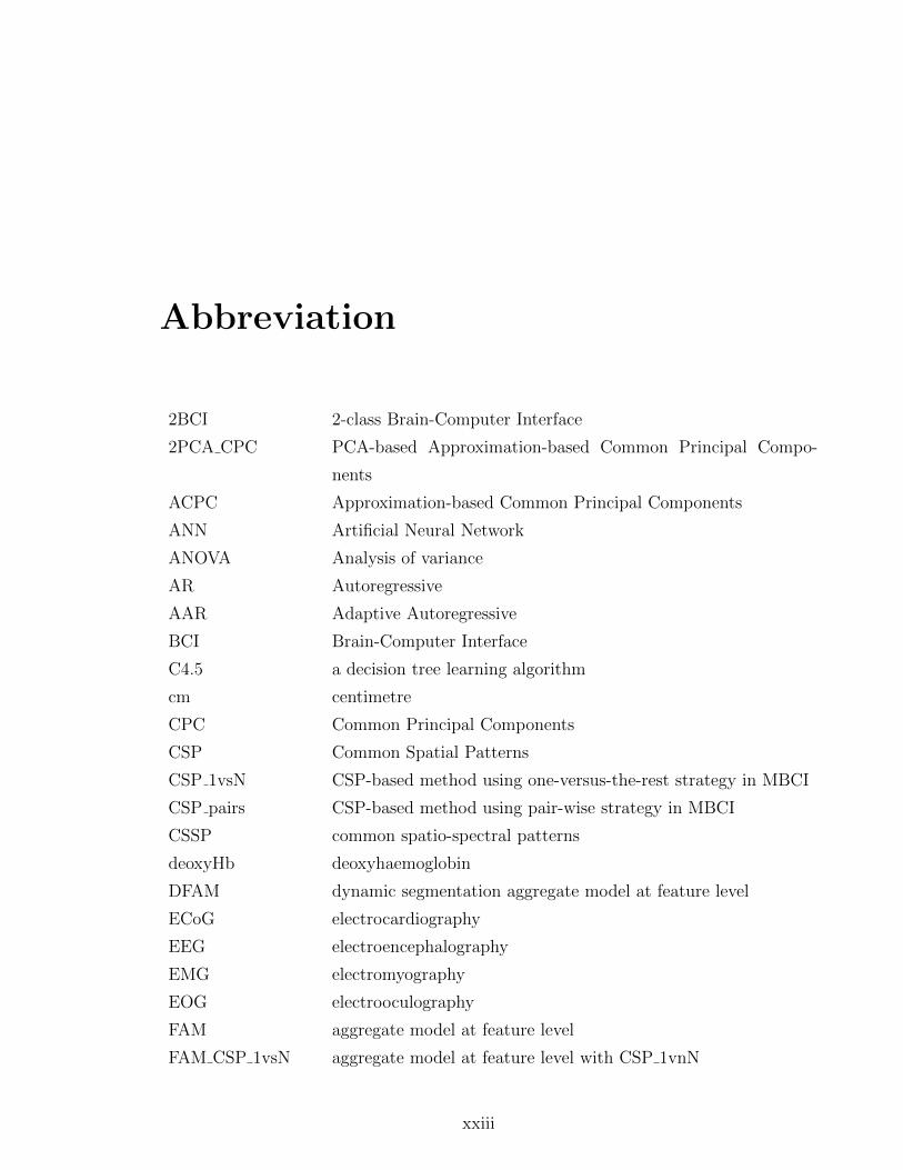
Abbreviation
2BCI 2-class Brain-Computer Interface
2PCA CPC PCA-based Approximation-based Common Principal Compo-
nents
ACPC Approximation-based Common Principal Components
ANN Artificial Neural Network
ANOVA Analysis of variance
AR Autoregressive
AAR Adaptive Autoregressive
BCI Brain-Computer Interface
C4.5 a decision tree learning algorithm
cm centimetre
CPC Common Principal Components
CSP Common Spatial Patterns
CSP 1vsN CSP-based method using one-versus-the-rest strategy in MBCI
CSP pairs CSP-based method using pair-wise strategy in MBCI
CSSP common spatio-spectral patterns
deoxyHb deoxyhaemoglobin
DFAM dynamic segmentation aggregate model at feature level
ECoG electrocardiography
EEG electroencephalography
EMG electromyography
EOG electrooculography
FAM aggregate model at feature level
FAM CSP 1vsN aggregate model at feature level with CSP 1vnN
xxiii
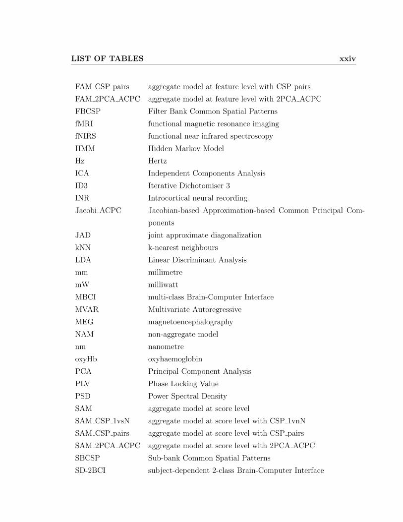
LIST OF TABLES xxiv
FAM CSP pairs aggregate model at feature level with CSP pairs
FAM 2PCA ACPC aggregate model at feature level with 2PCA ACPC
FBCSP Filter Bank Common Spatial Patterns
fMRI functional magnetic resonance imaging
fNIRS functional near infrared spectroscopy
HMM Hidden Markov Model
Hz Hertz
ICA Independent Components Analysis
ID3 Iterative Dichotomiser 3
INR Introcortical neural recording
Jacobi ACPC Jacobian-based Approximation-based Common Principal Com-
ponents
JAD joint approximate diagonalization
kNN k-nearest neighbours
LDA Linear Discriminant Analysis
mm millimetre
mW milliwatt
MBCI multi-class Brain-Computer Interface
MVAR Multivariate Autoregressive
MEG magnetoencephalography
NAM non-aggregate model
nm nanometre
oxyHb oxyhaemoglobin
PCA Principal Component Analysis
PLV Phase Locking Value
PSD Power Spectral Density
SAM aggregate model at score level
SAM CSP 1vsN aggregate model at score level with CSP 1vnN
SAM CSP pairs aggregate model at score level with CSP pairs
SAM 2PCA ACPC aggregate model at score level with 2PCA ACPC
SBCSP Sub-bank Common Spatial Patterns
SD-2BCI subject-dependent 2-class Brain-Computer Interface

LIST OF TABLES xxv
SD-MBCI subject-dependent multi-class Brain-Computer Interface
SD-BCI subject-dependent Brain-Computer Interface
SI-2BCI subject-independent 2-class Brain-Computer Interface
SI-BCI subject-independent Brain-Computer Interface
SI-MBCI subject-independent multi-class Brain-Computer Interface
SNR signal-to-noise ratio
SSF segmented spatial filters
SVM Support Vector Machine
UCPC Union-based Common Principal Components

List of Symbols
Fx the Fourier transform of the signal x
F ∗x complex conjunction of the Fourier transform of the signal x
| x | amplitude of complex number x
cxy cross-correlation function of signal x and signal y according to
time lag τ
x mean of signal x
δx variance of signal x
Cxy(ω) cross-spectrum of signal x and y
Ri(x) average distance from data point ith to other data points in an
embedding space constructed from signal x
Rpi (x) average distance from data point ith to its p nearest data points
in an embedding space constructed from signal x
Rpi (x|y) average distance from data point ith in embedding space con-
structed from x to p nearest data points of data point ith in an
embedding space constructed from signal y
Γxy(ω) coherence function of signal x and y
Sp(x|y) nonlinear interdependence measure of signal x given signal y con-
sidering p nearest data points
Hp(x|y) nonlinear interdependence measure of signal x given signal y con-
sidering p nearest data points
Np(x|y) normalized version Hp(x|y)
MI(x, y) mutual information of signal x and y
Entropy(Se) entropy of a set Se of samples
Entropy(x) entropy of signal x
xxvii

LIST OF TABLES xxviii
Entropy(x, y) joint entropy of signal x and y
K number of channels
Time number of sampled time points in a trial
t sample index or time index
Sub set of subjects
i index of a set
s a subject participating in a BCI experiment
X a set of trials in a dataset
Xi the i− th trial of dataset X
XCSPi projection of the i− th trial in CSP space
XCPCi projection of the i− th trial in CPC space
Lab(Xi) The known class label of trial Xi
z feature vector
zk k-th component of feature vector
κ Kappa coeeficient
Col(x, y) value at the point (x, y) in a grid
Aj,λ optical density of the j − th channel at wavelength λ
∆oxyj relative concentration changes of oxy-generated haemoglobin of
the j − th channel
∆deoxyj relative concentration changes of deoxy-generated haemoglobin
of the j − th channel
w window size or frame size
s window step or frame rate
argc(f) argument function which returns the argument c satisfying func-
tion f
argmaxc(f) maximize function f by tuning parameter c
argminc(f) minimize function f by tuning parameter c
L(x) aggregate function of signal x
c a class label
Fr(x) set of frames extracted from the signal x
frk the k-th frame of some frame set
SVM trained classifier using Support Vector Machines method

LIST OF TABLES xxix
Th threshold to determine predicted class in aggregate model
Cl general trained classifier
sign(.) sign function which returns sign of its argument
Dt weight set or a distribution over a training dataset in boosting
method
ht weak classifier at time point t
εt error of weak classifier at time point t over the training dataset
αt weighted coefficient used to combine weak classifiers to form the
final classifier
H(x) the final classifier in boosting method
Aj j − th component of feature space or j − th attribute
Chapter 1
Introduction
1.1 Research context
Brain-Computer Interface (BCI) is an emerging research field attracting a great deal
of effort from researchers around the world. Its aim is to build a new communication
channel that allows a person to send commands to an electronic device using his/her
brain activities [Wolpaw et al., 2002]. BCI systems have been provided to severely
handicapped people and patients with brain diseases such as epilepsy, dementia and
sleeping disorders [Lotte, 2008] for them to interact with other electronic devices.
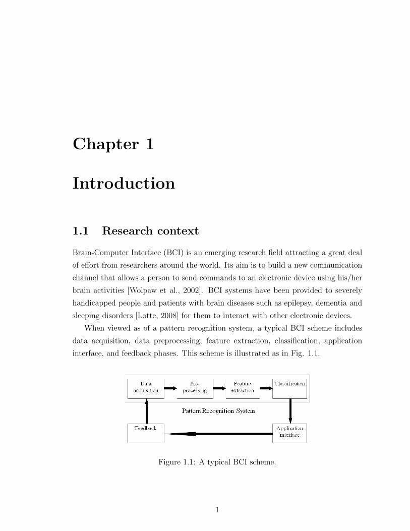
When viewed as of a pattern recognition system, a typical BCI scheme includes
data acquisition, data preprocessing, feature extraction, classification, application
interface, and feedback phases. This scheme is illustrated as in Fig. 1.1.
Figure 1.1: A typical BCI scheme.
1
1.1 Research context 2
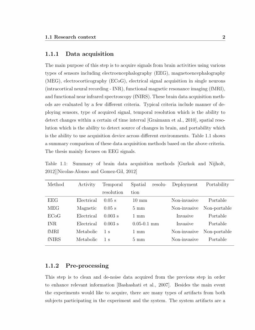
1.1.1 Data acquisition
The main purpose of this step is to acquire signals from brain activities using various
types of sensors including electroencephalography (EEG), magnetoencephalography
(MEG), electrocorticography (ECoG), electrical signal acquisition in single neurons
(intracortical neural recording - INR), functional magnetic resonance imaging (fMRI),
and functional near infrared spectroscopy (fNIRS). These brain data acquisition meth-
ods are evaluated by a few different criteria. Typical criteria include manner of de-
ploying sensors, type of acquired signal, temporal resolution which is the ability to
detect changes within a certain of time interval [Graimann et al., 2010], spatial reso-
lution which is the ability to detect source of changes in brain, and portability which
is the ability to use acquisition device across different environments. Table 1.1 shows
a summary comparison of these data acquisition methods based on the above criteria.
The thesis mainly focuses on EEG signals.
Table 1.1: Summary of brain data acquisition methods [Gurkok and Nijholt,
2012][Nicolas-Alonso and Gomez-Gil, 2012]
Method Activity Temporal
resolution
Spatial resolu-
tion
Deployment Portability
EEG Electrical 0.05 s 10 mm Non-invasive Portable
MEG Magnetic 0.05 s 5 mm Non-invasive Non-portable
ECoG Electrical 0.003 s 1 mm Invasive Portable
INR Electrical 0.003 s 0.05-0.1 mm Invasive Portable
fMRI Metabolic 1 s 1 mm Non-invasive Non-portable
fNIRS Metabolic 1 s 5 mm Non-invasive Portable
1.1.2 Pre-processing
This step is to clean and de-noise data acquired from the previous step in order
to enhance relevant information [Bashashati et al., 2007]. Besides the main event
the experiments would like to acquire, there are many types of artifacts from both
subjects participating in the experiment and the system. The system artifacts are a

1.1 Research context 3
50/60 Hz power supply interference, electrical noise from electronic components, and
cable defects. The subject artifacts are body-movement related to electrooculography
(EOG), electromyography (EMG), electrocardiography (ECG), and sweating. These
artifacts make the recorded EEG signal to have a low signal-to-noise ratio (SNR).
1.1.3 Feature extraction
Feature extraction is a crucial step in the BCI scheme. Its task is to represent the
whole signal by using some shorter and more meaningful measures called features
[Bashashati et al., 2007][Lotte et al., 2007]. Until now, although there has been a lot
of effort from neuroscientists seeking to discover brain and neural operations inside
it, the overall knowledge of human-beings about the brain is still very limited. This
shortcoming makes brain signal more difficult than other signals such as voice signal
in feature extraction.
1.1.4 Classification
The task of the classification step is to assign an object represented by a feature
vector to a class. In a BCI system, classes are usually brain states or, subject real
or imaginary actions. One of the most important challenges of BCI systems is that,
due to difficulties in setting up experiments, sample data used for the training phase
is quite small compared with the feature vector size. Thus, trained classifiers are
easy to become overfit. Researchers have tried to apply a number of classifiers [Lotte
et al., 2007], both linear and non-linear. Some well known and successful methods are
Linear Discriminant Analysis (LDA), Principal Component Analysis (PCA), Support
Vector Machine (SVM), Hidden Markov Model (HMM), k-nearest neighbours (kNN)
and Artificial Neural Network (ANN). Among them, LDA and SVM are the two best
classifiers [Lotte et al., 2007].
1.1.5 Application interface
After correctly identifying brain state or brain activity, the results of the classifier are
converted into some command sets which will be sent to control devices. This step
depends on the specific electronic device and application.

1.2 Brief introduction to EEG-based BCI systems 4
1.1.6 Feedback
Feedback is the last step helping users control their brain activity and in this way this
improve the BCI system’s performance. Usually, it provides the user with feedback
about brain states. In most BCI systems, the feedback step is used in the training
phase or offline phase [Lotte, 2008].
1.2 Brief introduction to EEG-based BCI systems
A BCI system can be classified as an invasive or non-invasive BCI according to the
way the brain activity is being measured within this BCI. If the sensors used for
measurement are placed within the brain, i.e. under the skull, the BCI is said to be
invasive. By comparison, if the measurement sensors are placed outside the head,
on the scalp for instance, the BCI is said to be non-invasive [Lotte, 2008]. The
non-invasive BCI systems avoid health risks and associated ethical concerns. In the
case of normal people, it is easy to see that invasive methods are not a good choice.
Furthermore, non-portable methods limit flexibility of these systems [Cichocki et al.,
2008][Moore, 2003][Wolpaw et al., 2006]. From Table 1.1 it can be seen that EEG
and fNIRS are the best candidates for an acceptable BCI system. Comparing these
two methods, fNIRS is less portable and more expensive than EEG, and it provides
a much lower temporal resolution which is very important in real time BCI systems.
Consequently, EEG is the most popular brain data acquisition method used in BCI
systems. Following this trend, the thesis focus is on EEG-based BCI systems.
Modern EEG recording systems consist of a number of small and soft electrodes, a
set of differential amplifiers (one for each channel) with filters, and pen-type registers.
When using with a large number of electrodes, electrode caps are the best choice. The
International Federation of Societies for Electroencephalography and Clinical Neuro-
physiology has recommended a standard 10-20 system (Fig. 1.2) for 21 electrodes. In
this setting, the standard considers some constant distance and uses 10% or 20% of
that one as the electrode interval. Each electrode is named based on its position in
relation to brain region.
Depending on the human state and/or age, an EEG signal contains different fre-
quencies and amplitudes. There are five major brain waves which differentiate from

1.2 Brief introduction to EEG-based BCI systems 5
Figure 1.2: Conventional 10-20 EEG electrode positions for 21 electrodes [Sanei and
Chambers, 2007].
1.2 Brief introduction to EEG-based BCI systems 6
each other by their frequency spectrum [Nicolas-Alonso and Gomez-Gil, 2012][Gurkok
and Nijholt, 2012][Sanei and Chambers, 2007]. They are called alpha (α), theta (θ),
beta (β), delta (δ), and gamma (γ). Alpha waves are usually detected over the oc-
cipital region of the brain: their frequencies range from 8Hz to 13Hz. These waves
indicate a relaxed state when there is no attention or concentration. Beta waves are
mainly found over the frontal and central regions. Their frequencies range from 14Hz
to 30Hz, although in some of the literature there is no specified upper bound of a
beta wave’s frequency. When people are in active thinking, active attention, focusing
on something, or solving problems, beta waves are generated. Beta waves are also
found when people are in a panic state. Delta waves lie within the range of 0.5 - 4Hz.
They are primarily associated with deep sleep or the waking up state of the human
brain. Theta waves have the range of 4 - 8Hz. They are associated with unconscious
material, creative inspiration, and deep meditation. The theta wave plays an impor-
tant role in infancy and childhood. Gamma waves, sometimes called fast beta waves,
have frequencies greater than 30Hz. These rhythms are used to confirm some brain
diseases. They are also used for locating some movement such as tongue, left and
right index fingers, and right toes.
A cognitive task will trigger a lot of simultaneous phenomena in the brain. Due
to human’s limited understanding of brain operation, most of these phenomena are
incomprehensive and cannot be traced to their origins. However, a few have been
decoded and therefore can be used in interpreting brain activity, which leads to their
use in BCI systems. In BCI systems, these signals are called control signals. There
are two main types of control signals: evoked signals and spontaneous signals [Lotte,
2008]. Evoked signals are generated unconsciously when a subject acknowledges a
specific stimulus. They are also called evoked potentials. Their main advantage
compared with spontaneous signals is that there is no need of a subject trained before
interacting with a BCI system. Evoked signals also can achieve a higher information
transfer rate than the spontaneous signals. Steady State Evoked Potentials (SSEP)
and P300 fall into this type of control signal. Spontaneous signals are intentionally
generated by the subject without any external stimulus due to an internal cognitive
process. To use these control signals in a BCI system needs quite an amount of
training time. Moreover, they achieve a lower information transfer rate than the first
1.2 Brief introduction to EEG-based BCI systems 7
type of control signal. However, they can provide a natural way for normal people to
communicate with BCI systems. Motor and sensorimotor rhythms, and slow cortical
potentials fall into this type of control signals. They are much less annoying than
evoked signals which are based on infrequent stimulus. Here, in this thesis the focus
is on motor-imagery control signal in EEG-based BCI systems. From now on, the
thesis uses the term BCI systems when referring to motor imagery EEG-based BCI
systems. Although there are some cases in which the thesis uses motor imagery-based
BCI systems as an alternative.
More formally, let X = {x} be a set of brain signals, Sub = {s} be a set of
subjects who generate X, and Lab = {l} be a set of class brain imagery or non-
imagery actions, the aim of BCI problems is to estimate the probability of class label
l happening given the signal x, denoting P (l|x). The probability distribution P can
be used for constructing classifiers later.
If the cardinal of the set Lab equals 2, we have 2-class BCI (2BCI) systems.
Otherwise, if the cardinal of the set Lab is greater than 2, we have multi-class BCI
(MBCI) systems.
If we estimate P (Lab|X) independent of subjects in Sub, we have subject-independent
BCI (SI-BCI) systems. Otherwise, if P (Lab|X) is individually estimated for each sub-
ject in Sub, we have subject-dependent BCI (SD-BCI) systems.
Combining these, in total we can classify BCI systems into four categories: subject-
dependent 2-class BCI (SD-2BCI) systems, subject-dependent multi-class BCI (SD-
MBCI) systems, subject-independent 2-class BCI (SI-2BCI) systems, and subject-
independent multi-class BCI (SI-MBCI) systems.
According to the BCI scheme described above, there are three main ways to im-
prove performance of a BCI system: enhancing quality of recording data at the data
acquisition step, analysing and proposing new features and capturing more relevant
information from brain activity at the feature extraction step, and choosing appro-
priate and improving classifiers at the classification step. Using the first way requires
improving sensor technology which is not the purpose of this research. For the third
way, numerous classifiers [Lotte et al., 2007] have been analyzed but the performance
of those BCI systems is still far from what is acceptable. On a standard dataset, the
data set IV of the BCI Competition 2003, Lotte et al. [Lotte et al., 2007] tried with
1.3 Problem statement 8
different classifiers accompanying with various features. The classification accuracy
ranges from 83% to 90%. Moreover, because the size of training data is quite small
[Lotte, 2008], researchers have few options but to choose classifiers which deal well
with small sample datasets. These arguments lead the research to choose feature
extraction as the main topic of this research. Due to the fact that features contain-
ing information extracted from the original signal, feature extraction methods are
believed to help researchers in explaining signals. Therefore, on the way to proposing
new features, the research can gain more knowledge about how the brain is organized
and operates.
1.3 Problem statement
The thesis is motivated by the aims to address four gaps in current research on BCI.
The first research gap is in synchronization measures. Quian et al. [Quiroga et al.,
2002] listed three reasons for considering synchronization measures. Firstly, they
allow assessment of the level of functional connectivity between two brain areas. Sec-
ondly, they have clinical relevance to identify different brain states and pathological
activities. Thirdly, they may show level of communication between different brain
areas. Recent studies [Varela et al., 2001], [Fiebach et al., 2005] revealed the great
importance of the coupling of brain regions referring to ”long-range synchroniza-
tion” of activities between distant brain regions. Although synchronization measures
have strong support from the results of clinical experiments, applying them in the
BCI research area is still at the beginning phase with little research undertaken to
date [Anderson et al., 1998], [Quiroga et al., 2002], [Nolte et al., 2004], [Schlogl and
Supp, 2006], [Brunner et al., 2010]. One of the successful synchronization measures
is Common Spatial Patterns [Blankertz et al., 2008b] which explores the properties
of covariance matrices. The second research gap is in multi-class BCI systems. For
problems which have less than 4 mental tasks, the BCI systems’ accuracies can be
up to 90%, but for the others, their accuracies quickly decrease [Obermaier et al.,
2001a]. A third research gap for multi-class BCI systems is that most of the cur-
rent approaches [Dornhege et al., 2004][Grosse-Wentrup and Buss, 2008][Wei et al.,
2010][Ang et al., 2012] convert the multi-class classification problem to a set of 2-

1.4 Targets of the research and brief of methodology 9
class classification problems. They do not directly target multi-class BCI systems.
The final gap in current research on BCI that is addressed in subject-independent
BCI systems. Due to the large inter-subject and inter-session variability, most of the
recent works focus on subject-dependent BCI systems. The large variability has its
root in the activation and delay issue in conducting BCI systems. It is a well-known
issue [Macaluso et al., 2007], [Toni et al., 1999]: the times of stimulation and response
which are expected to be the same or nearly the same, are actually different. As a
result, there are only a few works [Krauledat et al., 2008], [Fazli et al., 2009], [Lotte
et al., 2009] on SI-BCI systems up to now.
In summary, the research topic is about finding new methods for extracting syn-
chronization measures in multi-class BCI systems based on motor imagery in cares of
both subject-dependent and subject-independent systems.
1.4 Targets of the research and brief of methodol-
ogy
1.4.1 Targets of the research
As stated in the previous sections, the research focuses on finding new methods for
extracting features in motor imagery-based MBCI systems. This research limits the
scope of the research to BCI systems which use EEG as a mean of acquiring input
signals, although there is other technology that can be used for analyzing experiments
such as fNIRS. With these limitations in research scope, the thesis addresses three
research questions.
1. How can we build a feature extraction method based on synchronization mea-
sures that targets multi-class BCI systems directly instead of through a set of
2-class problems?
2. How can we build a feature extraction method that overcomes the issue of large
inter-subject and inter-session variability in multi-class BCI systems?
3. What is the difference in performance between subject-dependent and subject-
independent MBCI systems? What feature extraction methods can be used in

1.5 The thesis outline 10
subject-independent MBCI systems for enhancing performance? What models
can be used in both subject-dependent and subject-independent MBCI systems?
1.4.2 Brief of Methodology
As discussed so far, the study views BCI systems as pattern recognition problems
which include four steps: data acquisition, data pre-processing, feature extraction
and classification. Thus, the research can employ a large number of research methods
published in the pattern recognition area. But also, there is the fact that CSP anal-
ysis based on covariance analysis is the state-of-the-art method for feature extraction
in motor-imagery BCI systems. Thus, the research will focus on covariance matri-
ces in analyzing synchronization measures. On the way to finding answers for the
research questions, experiments were conducted on both EEG and fNIRS to analyze
brain signals. To validate these methods, well-known public standard EEG datasets
were used in the experiments. In this way, the time for conducting complicated ex-
periments very carefully was reduces. Dataset 2a of the BCI Competition IV which is
one of the most popular multi-subject multi-class benchmark datasets in BCI research
was used as the main dataset for validation in the research.
1.5 The thesis outline
The thesis is organized as follows. Chapter 1 introduces the research context, the
scope of the research, the problem statement and aims of the research. In Chapter 2,
the thesis reviews the relevant literature in BCI systems generally, and, specifically
their feature extraction methods. In Chapter 3, the problem of multi-class is for-
malized, the base-line methods which were later used to compare with the proposed
methods are introduced. In Chapter 4, a new method was proposed for feature ex-
traction called Approximation-based Common Principal Components (ACPC) which
directly deals with multi-class BCI systems. Chapter 5 presents the experimental re-
sults of two implementations of the proposed ACPC method. It also contains a
discussion related to the ACPC method. In Chapter 6, two general aggregate mod-
els are proposed to deal with inter-subject and inter-session variability in multi-class
BCI systems. The thesis discusses in detail these models when combined with ACPC

1.5 The thesis outline 11
as the feature extractor and prove that these methods can work well for both subject-
dependent MBCI systems and subject-independent MBCI systems. The experimental
results and related discussions are in Chapter 7. And finally, in Chapter 8, the con-
clusions are presented and possible directions for future research are proposed.

Chapter 2
Literature Review
In this chapter, relevant literature on BCI is reviewed. It covers details of the com-
ponents of BCI, including data acquisition, types of control signal, pre-processing
techniques, feature extraction and classifiers. For each component, there is a review
and comparison made with existing methods in use. Then, choices for specific com-
ponents in the research’s experiments are identified and explained. While reviewing
all phases in BCI systems, the chapter pays most attention to the feature extraction
phase due to it being the thesis topic. After reviewing the feature extraction methods,
the reasons and necessary of conducting this research are explained.
2.1 Brain-Computer Interface
A Brain-Computer Interface (BCI) which is also often referred as Brain-Machine In-
terface is a communication system that enables humans to interact with other devices
using their brain activity rather than their peripheral nerves and muscles [Wolpaw
et al., 2002]. Due to this characteristic, BCI systems have a huge attraction from
people who suffer from sever motor disabilities. Successful BCI applications not only
improve these people’s lives but also reduce the cost of intensive care. Until recently
BCI had very little attraction for researchers. There were only three groups in the
world investigate BCI research twenty five years ago and about ten groups fifteen years
ago[Wolpaw, 2007]. People believed that designing BCIs was too complex because of
many factors including limited resolution, reliability of detectable information from
13

2.1 Brain-Computer Interface 14
the brain, the high variability of acquired signals, and the constraints of extremely
expensive devices [Nicolas-Alonso and Gomez-Gil, 2012]. The situation is getting
better. BCI research is now considered a young multidisciplinary field integrating
researchers and knowledge from neuroscience, physiology, psychology, biomedical en-
gineering and computer science [Nicolas-Alonso and Gomez-Gil, 2012]. Number of
groups doing BCI research significantly increases over last 15 years. There are more
than 100 groups doing BCI research in 2007 [Wolpaw, 2007]. Nevertheless, most BCI
systems are under developed and in a laboratory stage only. Although there are some
specialized BCI products now on the shelf that are oriented toward public users such
as of Emotiv [Emotiv, 2013] or Neurosky [Neurosky, 2013] for example.
A typical BCI system operates as follows. Firstly, a user is asked to perform
some brain activity. The activity is then acquired and quantified as a brain signal.
Secondly, the brain signal is prepared and processed. Through this processing relevant
information is extracted from the brain signal. Thirdly, the relevant information
is used to interpret and obtain knowledge on the user’s mental state or intention.
Finally, this knowledge is used to communicate with other devices. From view point
of a pattern recognition system, a general BCI system includes data acquisition, data
preprocessing, feature extraction, classification, application interface, and feedback
phases. This scheme is illustrated as in Fig. 1.1. The following subsections review in
more detail these phases in BCI systems.
2.1.1 Data acquisition in BCI
Data acquisition technologies for measuring brain activity can be categorized into two
main categories: those that use electrophysiological and those that use hemodynamic
methods [Nicolas-Alonso and Gomez-Gil, 2012][Gurkok and Nijholt, 2012]. Electro-
physiological methods rely on a well-known electro-chemical process inside the brain.
Basically, neurons will generate ionic currents when exchanging information with oth-
ers. By measuring these currents, researchers believe that they can know about the
exchanged information or the brain activity. Methods that fall into this electrophysi-
ological group include electroencephalography (EEG), electrocorticography (ECoG),
magnetoencephalography (MEG), and electrical signal acquisition in single neurons
(intracortical neural recording - INR). Hemodynamic methods are based on a pro-
2.1 Brain-Computer Interface 15
cess in which the ratio of oxyhemoglobin to deoxyhemoglobin changes in active brain
area. These changes are due to the blood releasing more glucose and oxygen in an ac-
tive brain area than other inactive ones. This hemodynamic group includes methods
such as functional magnetic resonance imaging(fMRI) and functional near infrared
spectroscopy (fNIRS).
These brain data acquisition methods are evaluated using different criteria [Nicolas-
Alonso and Gomez-Gil, 2012][Gurkok and Nijholt, 2012]. Typical criteria are the
manner of deploying sensors, type of acquired signal, temporal resolution, spatial res-
olution, and portability. There are two manners of deploying sensors: invasive and
non-invasive. While invasive methods require some level of brain surgery to place
sensors inside the skull, non-invasive methods do not. Invasive methods are therefore
considered extremely risky and only used for people with severe motor disabilities.
Specifically, ECoG and electrical signal acquisition in single neurons are invasive meth-
ods. The others are non-invasive methods measure signal from the scalp. The types
of acquired signal are electrophysiological and hemodynamic. Electrophysiological
signals can be further divided into electrical and magnetic. Specifically, EEG, ECoG
and INR measure electrical activity, and MEG measures magnetic activity. Hemo-
dynamic or metabolic activity is measured by fMRI and fNIRS. Temporal resolution
and spatial resolution refer to how precisely a method can measure in the tempo-
ral domain and the spatial domain, respectively. Invasive methods usually produce
brain images with better temporal and spatial resolution. On the other hand, due
to spatial mixing of generated activity from different cortical areas and the absorb-
tion of signals from brain tissues, bone and skin, non-invasive methods provide quite
low spatial resolution. Among non-invasive methods, EEG and MEG provide the
best temporal resolution, while fMRI provides the best spatial resolution. Portability
represents how portable a data acquisition method is. EEG, ECoG and fNIRS are
more portable than the others. A summary of these brain data acquisition methods
is shown in Table 1.1.
When considering a BCI system for normal people, it is easy to see that invasive
methods are not a good choice. Furthermore, non-portable methods will limit the
flexibility of these systems. EEG and fNIRS are therefore the best candidates for BCI
systems. Comparing these two methods, fNIRS is less portable and more expensive

2.1 Brain-Computer Interface 16
than EEG, and provides a much lower temporal resolution which is very important in
real time BCI systems. Consequently, EEG is the most popular brain data acquisition
method used in BCI systems. Following this trend, the research focuses on EEG-based
BCI systems.
The first reported attempt to measure human brain activity using EEG was that
undertaken by Hans Berger in 1924 [Lotte, 2008]. It was also the first time people mea-
sured human brain activity altogether. In his work, Berger used electroencephalogra-
phy (EEG) to measure the sum of potentials generated by thousands of neurons inside
the brain through electrodes placed on the scalp. The acquired electrical signal using
EEG is very weak so it needs to be strongly amplified before processing. Depending
on the purpose and expert knowledge of BCI systems, designers of BCI determine
the number of electrodes used in experiments. This number varies from 1 to 256
electrodes in reported BCI systems [Lotte, 2008]. To make it easy for setting and
comparing experiments, electrode positions on the scalp are standardized. According
to the 10-20 international system [Jasper, 1958][Sharbrough et al., 1991](Fig. 1.2),
each position has coordinates and a name.
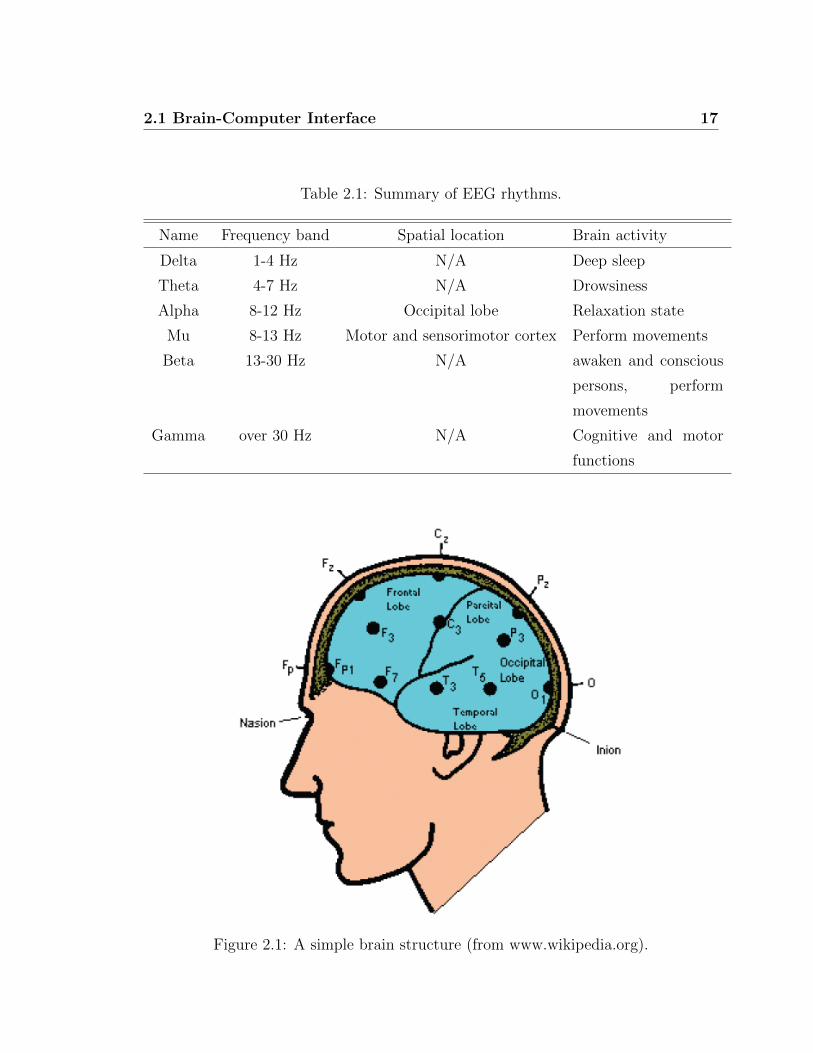
EEG signals are composed of different rhythms. These rhythms differ from each
other by their spatial and spectral localization. They are also different in purpose of
brain activity. Table 2.1 summarizes six classical EEG rhythms in their names, spa-
tial localization, frequency band (spectral localization) and typical associated brain
activity. Fig. 2.1 shows a simple structure of brain.
2.1.2 Types of control signal in BCI
A cognitive task will trigger a great many simultaneous phenomena in brain. Due
to human’s limited understanding of the brain’s operation, most of these phenomena
are incomprehensible and cannot be traced to their origins. However, a few of them
have been decoded and therefore can be used in interpreting brain activity, thus their
usage in BCI systems. These signals are called control signals in BCI systems. There
are two main types of control signals: evoked signals and spontaneous signals [Lotte,
2008]. Evoked signals are generated unconsciously when a subject acknowledges a
specific stimulus. They are also called evoked potentials. Their main advantage when
compared with spontaneous signals is that they do not need subjects trained before
2.1 Brain-Computer Interface 17
Table 2.1: Summary of EEG rhythms.
Name Frequency band Spatial location Brain activity
Delta 1-4 Hz N/A Deep sleep
Theta 4-7 Hz N/A Drowsiness
Alpha 8-12 Hz Occipital lobe Relaxation state
Mu 8-13 Hz Motor and sensorimotor cortex Perform movements
Beta 13-30 Hz N/A awaken and conscious
persons, perform
movements
Gamma over 30 Hz N/A Cognitive and motor
functions
Figure 2.1: A simple brain structure (from www.wikipedia.org).
2.1 Brain-Computer Interface 18
they interact with BCI systems. They also can achieve a higher information transfer
rate than the spontaneous signals. Steady State Evoked Potentials (SSEP) and P300
fall into this type of control signal. Spontaneous signals are intentionally generated
by the subject without any external stimulus due to an internal cognitive process.
When using these control signals in BCI, quite a large amount of training time is
needed. Moreover, these control signals achieve a lower information transfer rate
than the first type. However, they can provide a natural way for normal subjects to
communicate with BCI systems. Motor and sensorimotor rhythms, and slow cortical
potentials fall into this type of control signal. They are much less annoying than
evoked signals which are based on infrequent stimulus. This was one reason for this
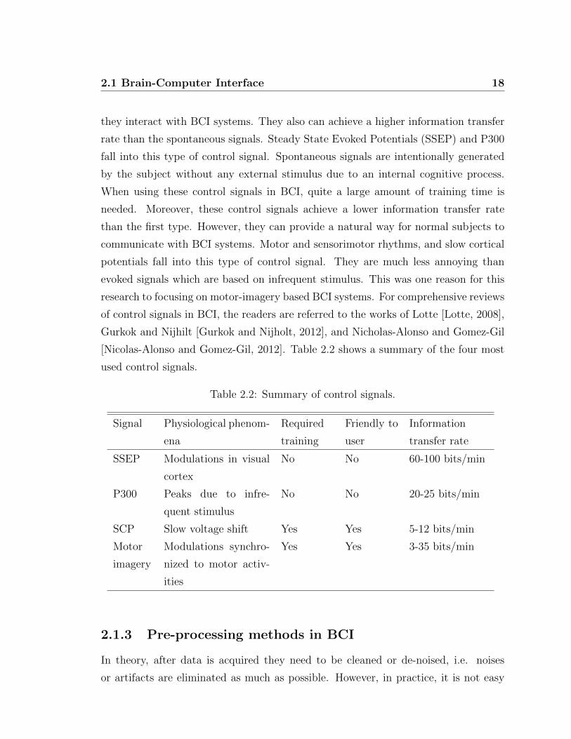
research to focusing on motor-imagery based BCI systems. For comprehensive reviews
of control signals in BCI, the readers are referred to the works of Lotte [Lotte, 2008],
Gurkok and Nijhilt [Gurkok and Nijholt, 2012], and Nicholas-Alonso and Gomez-Gil
[Nicolas-Alonso and Gomez-Gil, 2012]. Table 2.2 shows a summary of the four most
used control signals.
Table 2.2: Summary of control signals.
Signal Physiological phenom-
ena
Required
training
Friendly to
user
Information
transfer rate
SSEP Modulations in visual
cortex
No No 60-100 bits/min
P300 Peaks due to infre-
quent stimulus
No No 20-25 bits/min
SCP Slow voltage shift Yes Yes 5-12 bits/min
Motor
imagery
Modulations synchro-
nized to motor activ-
ities
Yes Yes 3-35 bits/min
2.1.3 Pre-processing methods in BCI
In theory, after data is acquired they need to be cleaned or de-noised, i.e. noises
or artifacts are eliminated as much as possible. However, in practice, it is not easy
2.1 Brain-Computer Interface 19
to separate the pre-processing and feature extraction phases. In this research, pre-
processing methods are defined as methods that try to reduce noise or artifacts. By
this definition, pre-processing methods are artifact-removal methods only. There are
two typical methods for removing artifacts in BCI. Artifacts in EEG signals usually
come from muscular, ocular and heart activity [Fatourechi et al., 2007]. They are
named as electromyography (EMG), electrooculography (EOG), and electrocardiog-
raphy (ECG) artifacts, respectively. Artifacts also come from technical sources such as
power-line noises or changes in electrode impedances. The first method includes low-
pass or band-pass filters which are based on the Discrete Fourier Transform (DFT),
Finite Impulse Response (FIR) or Infinite Impulse Response (IIR) [Smith, 1997]. In
motor imagery-based BCI systems, low-pass or band-pass filters are usually used to
cut off irrelevant frequencies. This method is very efficient when dealing with techni-
cal artifacts. The second method widely used for removing artifacts is Independent
Component Analysis (ICA). This is a statistical method aimed at decomposing a
set of mixed signals into its sources. Pioneer work such as that of Vigario [Vigrio,
1997][Vigrio et al., 2000] has aimed at removing ocular artifacts from EEG signals.
While ICA has been proven a robust and powerful tool for removing artifacts in the
analysis of EEG signals [Fatourechi et al., 2007], reports from some authors suggest
that removing artifacts by using ICA may corrupt the power spectrum of the ana-
lyzed EEG signal [Wallstrom et al., 2004]. Furthermore, ICA requires that artifacts
be independent of the normal activity of the analyzed EEG signal. This requirement
is sometimes not easy to satisfy due to the complicated and relatively unknown op-
eration of the brain. In this research, only low-pass and band-pass filters were used
for pre-processing EEG signals.
2.1.4 Classifiers in BCI
The task of the classification step is to assign an object represented by a feature
vector to a class. Because, this thesis focused on the feature extraction phase of BCI
systems, details of feature extraction methods are reviewed in the next section. BCI
inherits many classifiers from the pattern recognition field. Researchers in BCI have
experimented with many classifiers in the classification phase. Typical and successful
classifiers include Linear Discriminant Analysis (LDA), Principal Component Analy-
2.1 Brain-Computer Interface 20
sis (PCA), Support Vector Machine (SVM), Hidden Markov Model (HMM), k-nearest
neighbours (kNN) and Artificial Neural Network (ANN). For a comprehensive review
of classifiers used in BCI, the readers is referred to the work of Lotte et al. [Lotte
et al., 2007]. Similar to other pattern recognition systems, classifiers in BCI systems
are faced with the well known problem of the curse of dimensionality. This means that
to train a good classifier, providing training data whose size increases exponentially
with the size of the feature vector is needed. As stated in the brain data acquisi-
tion phase, training in BCI is a time-consuming process and not a user friendly task.
Therefore, available training sets in BCI are usually small. This make classifiers in
BCI easy to overfit the training data. To overcome this problem, researchers tend to
choose classifiers which are robust in dealing with small training data. Lotte et al.
[Lotte et al., 2007] reported that among the classifiers they tried, LDA and SVM were
the best. The research reported here uses SVM as the classifier in the experimented
BCI systems due to its frequent and widespread used in BCI systems and multi-class
support.
The main idea of Support Vector Machine is that it tries to find hyperplanes in
order to both maximize the distance between the nearest training samples and the
hyperplanes and minimize the empirical risk. The nearest training samples are called
support vectors. Let {xi, yi}, xi ∈ Rd, i = 1, . . . , n be the training data set with two
labels yi ∈ {−1,+1}. Let φ be the transformation from the input space to the feature
space. The SVM will find the optimal hyperplane [Vapnik, 1995]
f(x) = wTφ(x) + b (2.1)
to separate the training data by solving the following optimisation problem:
minw,b
(1
2||w||2 + CF (
n∑i=1
ξi))
(2.2)
subject to
yi(wTφ(xi) + b) ≥ 1− ξi i = 1, . . . , n (2.3)
where w is the normal vector of the hyperplane, C and b are real numbers, ξi, i =
1, . . . , n are non-negative slack variables, and F is any monotonic convex function.

2.1 Brain-Computer Interface 21
Further the assumption of F (u) = u will rewrite the optimization problem in Eq.
(2.2) as follows:
minw,b
(1
2||w||2 + C
n∑i=1
ξi
)(2.4)
subject to
yi(wTφ(xi) + b) ≥ 1− ξi i = 1, . . . , n (2.5)
Krush-Kuhn-Tucker theory is then applied to solve the optimization in Eq. (2.4). For
more information about SVM, the readers are referred to the original work of Vapnik
[Vapnik, 1995].
2.1.5 Existing BCI Applications and Systems
While the origin purpose of BCI research is to provide a new communication channel
for people who are suffering from sever motor disabilities, BCI applications has been
not limited to application for disabilities but extend to for normal people. Nicholas-
Alonso et al. [Nicolas-Alonso and Gomez-Gil, 2012] targeted BCI applications to
three groups of user: Complete Locked-In State patients; Locked-In State patients;
and able-bodied people or those who can control their neuromuscular systems. The
applications for the last group are used to extract such as affective information which
is difficult to reveal if using different technologies. Nicholas-Alonso et al. [Nicolas-
Alonso and Gomez-Gil, 2012] went further to divide current BCI applications and
systems into six main categories including communication, motor restoration, envi-
ronmental control, locomotion, entertainment and others. While acknowledging a
huge potential market of these applications, the authors raise some concerns about
some ethical issues when BCI technology can be used to manipulate the brain and
consumer behaviour.
Almost BCI systems described above are wired. In these systems, communication
between the data acquisition component and other components is through wired
transmission. For some applications such as of locomotion, wired communication is
not flexible enough. Due to this reason, some researchers have been trying to develop
wireless-based BCI systems [Seungchan Lee, ].

2.2 Feature extraction in BCI systems 22
2.2 Feature extraction in BCI systems
2.2.1 Feature extraction in general BCI systems
Feature extraction in BCI systems is defined as a component ”that translates the
(artifact-free) input brain signal into a value correlated to the neurological phe-
nomenon” [Mason et al., 2007]. A feature, therefore, is defined as a value correlated
to the neurological phenomenon. The feature extraction is also called noise reduc-
tion or filtering. The output of feature extraction forms a feature vector which is
usually significantly shorter and contains more relevant information then the brain
input signal. The feature extraction methods fall into two main categories. The
first involves methods which use a single channel for extracting features. The second
involves methods which use information from more than one channel for extracting
features.
For an easy review of the features, let X = {x} be a set of brain signals which
have N channels, Sub = {s} be a set of subjects who generate X, and Lab = {l} be a
set of class brain imagery or non-imagery actions. The notations X(t) and x(t) were
used in order to emphasize the time-series property of the signal. The subscript i was
used with x when the thesis wanted to distinguish trials from each other. Without
any explanation, x was treated as a univariate signal. Otherwise, it was treated
as a multi-variate signal. Similarly, li and si were used when the thesis wanted to
distinguish class labels and subjects, respectively.
Single-channel feature extraction methods
A great number of features [Bashashati et al., 2007], [Lotte et al., 2007] have been
tried and applied on BCI systems. The most simple feature extracted from individual
channels is the amplitude of the signal or raw data [Hoffmann et al., 2005], [Rivet
and Souloumiac, 2007], [Sitaram et al., 2007], [Gottemukkula and Derakhshani, 2011].
Accompanied by other dimension reduction techniques such as sub-sampling, this kind
of simple feature can achieve quite a good performance in BCI systems which, however
are not based on motor imagery but on P300 [Hoffmann et al., 2005], [Rivet and
Souloumiac, 2007] or other data acquisition techniques such as functional near infrared
spectroscopy (fNIRS) [Sitaram et al., 2007], [Gottemukkula and Derakhshani, 2011].

2.2 Feature extraction in BCI systems 23
Obermeier [Obermaier et al., 2001a] attempted to use Hjorth parameters or Time
domain Parameters for the online classification of a right and left imagery problem.
They extracted Hjorth parameters including activity, mobility, and complexity from
channel C3 and C4 of a single trial EEG signal forming a 6-dimension feature vector
for each segment. A Hidden Markov Model was used as the classifier in their work.
Their system achieved accuracy of 81.4±12.8 in percentage terms. They concluded
that their system can be used in online motor imagery classification.
Activity(x(t)) = V AR(x(t)) (2.6)
Mobility(x(t)) =
√Activity(dx(t)
dt
Activity(x(t))(2.7)
Complexity(x(t)) =Mobility(dx(t)
dt)
Mobility(x(t))(2.8)
Band power features were used by Pfurtscheller et al. [Pfurtscheller et al., 1997] also
in a right and left imagery problem. They experimented on 3 subjects with a 128Hz
EEG recording. For each subject, different frequency components belong to alpha (α)
and beta (β) bands which contributed most on discrimination between two types of
movement. Their system achieved accuracy of approximately 80%. Later, Palaniap-
pan [Palaniappan, 2005], [Obermaier et al., 2001b] used spectral powers in several
BCI systems. In Palaniapan’s experiments, four subjects were asked to perform four
mental tasks with a 6-electrode EEG system. Spectral powers of four frequency bands
including delta and theta, alpha, beta and gamma of all 6 channels were calculated
and used as features which fed into a neural network classifier. They reported that
in single mental tasks, this system could achieve an accuracy up to 97.5% with the
most suitable mental task. There was no further report on 2-class or multi-class ex-
periments. By comparison, Obermeier et al. [Obermaier et al., 2001b] reported that
their system achieved at most an accuracy of 96% with 2 mental tasks and at most of
67% with 5 mental tasks. By using band power as features, Obermeier et al. aimed to
measure variance in some specific frequency bands and hoped that specific patterns
over different electrodes existed. They found that band power features are well suited
for motor-related problems such as motor imagery or motor execution tasks. There
is a link between band powers and Hjorth parameters. Navascues and Sebastian in
[Navascus and Sebastin, 2009] proved that derivatives of a signal could be represented

2.2 Feature extraction in BCI systems 24
by the signal’s spectral powers in the frequency domain. Consequently, the mobility
and complexity of a signal can be calculated based on the signal’s spectral powers.
Recently, Brodu et al. [Brodu et al., 2011] conducted an empirical experiment in
which band power estimation algorithm is the best one. They came to the conclusion
that, for a motor imagery task, the Morlet wavelet is the best algorithm to extract
band power information from an EEG signal.
Autoregressive (AR) model parameters and its adaptive version (AAR) are other
widely used features in BCI systems. The main purpose of the autoregressive model,
as shown in Eq.(2.9), is to estimate data at time t by a weighted sum of previous data
values and a noise term e(t). The adaptive autoregressive model extends the original
model by assuming that the weight ai can be varied over time instead being fixed.
Both of them depend on the parameter p which is called the order of the model.
x(t) =
p∑i=1
aix(t− i) + e(t) (2.9)
Researchers have tried to fit an EEG signal with a model as closely as possible so
that the model parameters ai can be used as features representing the corresponding
EEG signal. Penny et al. [Penny et al., 2000] used AR model parameters as features
to classify motor imagery tasks with an accuracy of 61% without the reject option
and 87% with the reject option. They used a Bayesian logistic regression model
as classifier. Obermeier [Obermaier et al., 2001a] tried AAR model parameters in
the same experiment with Hjorth parameters as features. Its accuracy was about
72.4±8.6%. Because they used AAR parameters with an LDA classifier there is no
possible comparison made between these two feature extraction methods. Tavakolian
et al. [Tavakolian et al., 2006] tried AAR parameters on well known dataset III of
the BCI Competition 2003 and found that the system’s accuracy was quite stable
at about 82-84% with different classifiers. The main advantage of the AR and AAR
model parameters is that they are parametric methods for feature extraction. By
adjusting their model orders, they can control the trade off between accuracy and
overfit issues.
Due to their easy computation, these linear features, including Hjorth parameters,
band powers and AR model parameters are popular and usually used as benchmarks
or in quick feedback sessions in BCI experiments. However, as noted above, these
2.2 Feature extraction in BCI systems 25
features cannot achieve the acceptable accuracy when they are used in multi-class
BCI systems.
Besides linear features, researchers have been trying non-linear features in BCI
systems. The first question they want answered is whether or not non-linear prop-
erties exist in brain signals. Andrejak and his co-workers [Andrzejak et al., 2001]
pointed out that there are some indications of nonlinear deterministic and finite-
dimensional structures in the time series of brain EEG signals depending on brain
region and brain state. They reported that there are strong indications of non-linear
deterministic dynamics for epilepsy seizure activity. For other brain tasks such as eye
opening or closing, there are less strong indications of non-linear properties. Based on
this work, Gautama et al. [Gautama et al., 2003] reconfirmed there were non-linear
indications in EEG brain signals and further proposed the Delay Vector Variance
method for use in classification tasks. They also proved that their proposed Delay
Vector Variance method outperforms the other two nonlinear methods named the
third-order autocovariance and the asymmetry due to time reversal. Although there
are signs of non-linear properties in brain signals, non-linear features are considered
less efficient than linear features in motor imagery EEG-based systems. For exam-
ple, Boostani et al. [Boostani and Moradi, 2004] conducted their experiments with
5 subjects in 6-electrode EEG recording systems for 2 motor imagery tasks. They
experimented with 3 features including band power, Hjorth parameters and Fractal
dimension. Their experimental results show that in the training phase, the Fractal
dimension feature was not as good as the Band Power feature. In the testing phase,
with a few specific subjects and at some specific tasks, the Fractal dimension can
achieve better accuracy. It is noted that the Fractal dimension feature was used with
an Adaboost classifier while the other two features were used with an LDA classi-
fier. Zhou et al. [Zhou et al., 2008] argued that by assuming linearity, Gaussianality
and minimum-phase within the EEG signals, most conventional feature extraction
methods based on band power or AR models focus only on frequency and power in-
formation; they ignore phase information which plays a very important role in the
process of generating EEG signals. They proposed using high order statistics ex-
tracted from bispectrum of EEG signals as features. These nonlinear features reflect
phase relationships between frequency components of the signal. To test their idea,

2.2 Feature extraction in BCI systems 26
the authors conducted experiments on the Graz BCI data set of the BCI Competition
2003 which has 280 trials with 2 mental tasks. They also experimented with different
classifiers including LDA, SVM and NN. Their results show that for all classifiers
used, their proposed features outperformed those of winners of the competition in
the same dataset. Sharing the idea of using information of power of the signal be-
tween different frequencies, a number of researchers have used power spectral density
(PSD) or power spectrum as features [Dressler et al., 2004], [Madan, 2005], [Cona
et al., 2009], [Lotte, 2008], [Lotte et al., 2009], [Lotte and Guan, 2011]. This feature
is now the most preferred feature used in BCI systems [Lotte, 2008]. Recent work
of Krusienski et al. [Krusienski et al., 2012] re-emphasizes that phase information
has been under-utilized in BCI research. The most favoured and widely used fea-
ture extracted from phase information is the phase locking value (PLV) proposed by
Lachaux et al. [Lachaux et al., 1999]. Gysels et al. [Gysels and Celka, 2004], Wei et
al. [Wei et al., 2007], and Krusienski et al. [Krusienski et al., 2012] are among the few
authors attempted to use PLV in BCI systems. Wei et al. [Wei et al., 2007] showed
that by combining phase information with other conventional features such as BP and
AR-based features they can enhance the performance of BCI systems. Later work of
Krusienski et al. in 2012 [Krusienski et al., 2012] has claimed a similar conclusion
namely that combining phase information with other spectral features extraction by
the Fast Fourier Transform or Magnitude-Squared Coherence can improve accuracy
of BCI systems. A further extension of the trend of utilizing information between
different frequencies has come to spatio-temporal models with data being analyzed
from both spectral and time domains at the same time. In this matter, wavelet anal-
ysis is the most popular technique and it has been applied in BCI systems. Wu et
al. [Ting et al., 2008] compared using wavelet packet decomposition as the feature
extraction method to other popular methods based on an AR model and Fast Fourier
Transform on a dataset of the BCI Competition 2003. They reported that wavelet
packet decomposition achieves promising results. Others [Sherwood and Derakhshani,
2009], [Asensio-Cubero et al., 2011] have tried to find out what types of wavelets are
suitable for BCI tasks. For motor imagery BCI systems, Sherwood [Sherwood and
Derakhshani, 2009] claimed that wavelet methods using sub-band energy were the
best. Asesino [Asensio-Cubero et al., 2011], on the other hand, believed that using
2.2 Feature extraction in BCI systems 27
genetic algorithms was a more suitable wavelet method for BCI tasks. A recent and
more comprehensive work comparing linear and nonlinear features was undertaken by
Balli and Palaniappan [Balli and Palaniappan, 2010] who analysed seven non-linear
features including: approximate entropy, largest Lyapunov exponents, correlation di-
mension, non-linear prediction error, Hurst exponent, higher order auto covariance,
and asymmetry due to time reversal in three biological signal datasets. These seven
non-linear features were compared with two linear features that based on the AR
model. They found that linear features such as AR model coefficients and AR re-
flection coefficients achieved higher accuracy than non-linear features and, that when
combining linear and non-linear features together they could achieve higher accuracy
than when done individually. Specifically, the combination of linear and nonlinear
features can improve by about 7.45% with the finger-movement EEG dataset and
6.62% with the epileptic EEG dataset. They drew the conclusion that a combination
of linear and nonlinear features could be a better approach for doing classification in
BCI systems. It can be seen that using non-linear features alone is not a good option
with BCI systems. Therefore, they are often used in combination with linear features
or in epileptic seizure detection EEG-based systems.
A summary of popular feature extraction methods based on individual channel is
provided in Table 2.3.
Multi-channel feature extraction methods
The above mentioned features do not take into account the coupling of brain regions.
A feature is extracted from a single channel does not capture the relations between
the channels in multichannel EEG recording systems. Such relations are believed to
be important in assessing the level of functional connectivity between the two brain
areas, identifying brain states and pathological activities as they contain clinical rel-
evance, and showing communication between different brain areas [Quiroga et al.,
2002]. In short, they could help researchers understand more about the brain and
its operation. Synchronous features or multivariate features have been proposed to
overcome this limitation. Actually, synchronization measures can be viewed as an
approach to improve the spatial resolution of EEG signals which is very low (≈ 1cm)
[Ariely and Berns, 2010]. Moreover, while the features described above are being

2.2 Feature extraction in BCI systems 28
Table 2.3: Summary of single channel feature extraction methods
Feature Feature
Type
Pros Cons
Raw data Raw Fast Low accuracy
Hjorth parame-
ters
Time
domain
Fast Low accuracy
Band power Frequency
domain
Fast, modest ac-
curacy
unsuitable for
multi-class
Autoregressive
model parame-
ters
Time
domain
Fast, parametric
method
Low accuracy
Power spectral
density
Frequency
domain
Fast, modest ac-
curacy
not high accu-
racy
Fractal dimen-
sion
Non-linear Fast Low accuracy
Phase informa-
tion
Non-linear Meaningful Low accuracy
2.2 Feature extraction in BCI systems 29
extracted from the temporal and frequency domains, synchronization measures are
providing information from the spatial domain. These multivariate features can be
categorized into two categories. The first contains the features which are directly
extracted through multivariate models such as multivariate autoregressive (MVAR)
parameters, bilinear AR parameters, non-linear inter-dependencies, phase synchro-
nization, mutual information, cross correlation and coherence function. The second
category features use multivariate models such as filters to enhance signals before
applying simple feature extraction in order to extract meaningful feature.
In regard to the first category, Quiroga et al. in their work [Quiroga et al., 2002]
analysed various synchronization features, including cross correlation (2.10), coher-
ence function (2.12), nonlinear inter-dependencies(2.13,2.14,2.15), phase synchroniza-
tion and mutual information(2.16), on three typical EEG datasets. They drew the
conclusion that synchronization measures can complement visual analysis and even
be of the clinical values.
cxy(τ) =1
N − τ
N−τ∑t=1
(x(t)− x
δx)(y(t+ τ)− y
δy) (2.10)
Cxy(ω) = Fx(ω)F ∗y (ω) (2.11)
Γxy(ω) =| Cxy(ω) |√
| Cxx(ω) || Cyy(ω) |(2.12)
Sp(x|y) =1
K
K∑i=1
logRpi (x)
Rpi (x|y)
(2.13)
Hp(x|y) =1
K
K∑i=1
logRi(x)
Rpi (x|y)
(2.14)
Np(x|y) =1
K
K∑i=1
Ri(x)−Rpi (x|y)
Ri(x)(2.15)
MI(x, y) = Entropy(x) + Entropy(y)− Entropy(x, y) (2.16)
Another approach for discovering spatial information from multichannel EEG signals
is using multivariate models. Schlogl et al. [Schlogl and Supp, 2006] used MVAR
parameters to analyze even-related EEG data. The typical formula of a multivariate
2.2 Feature extraction in BCI systems 30
autoregressive model is shown in Eq. (2.17). The only difference between equa-
tions (2.17) and (2.9) is that x, a and e respectively become d-dimensional, d-by-d-
dimensional and d-dimensional vectors.
x(t) =
p∑i=1
aix(t− i) + e(t) (2.17)
From MVAR parameters, Quiroga et al. derived several measures, including auto
and cross spectra, phase relations, coherency, partial coherence, partial directed co-
herence, direct transfer function, and full frequency direct transfer function. They did
not concentrate on analyzing performance improvement in the use of MVAR param-
eters. Instead, they focused on investigating various aspects of multichannel spectral
properties of EEG and attempted to explain interacting activity between different
brain areas. The authors concluded that MVAR is an feature easy to use for in-
vestigating such tasks. Nolte et al. [Nolte et al., 2004] used the imaginary part of
coherency to find out brain interaction when there is movement of subject from EEG
data. From a finger-movement EEG recording dataset, they found out two important
results. The first is that from about 5 seconds before through to movement onset,
there is a weak interaction of around 20Hz between left and right motor areas. The
second is that from about 2 to 4 seconds after movement, there is a stronger interac-
tion also at 20 Hz. These two interactions are in opposite directions. The researchers
concluded that it is possible to detect brain interaction during movement from EEG
data. Anderson et al. [Anderson et al., 1998] extracted multivariate autoregressive
model parameters from a 4-subject 2-mental task EEG dataset. They exploited four
features from 6 channels including AR model coefficients, MVAR model coefficients,
eigenvalues of correlation matrix, and the Karhunen-Loeve transformed version of the
second feature. All were fed them into a multi-layer neural network for classification.
The results showed that the four features achieved similar results but with the MVAR
feature slightly better and more consistent in the testing phase. It could achieve accu-
racy at 91.4% in the testing phase. Recently, in a comprehensive analysis by Brunner
et al. [Brunner et al., 2010], [Brunner et al., 2011] experiments were conducted to
compare various types of autoregressive model features for BCI including univari-
ate, multivariate, bilinear AR parameters, and logarithmic band power. They used
dataset 2a from the BCI Competition IV [Brunner et al., 2008], and suggested that

2.2 Feature extraction in BCI systems 31
there is no significant difference between AR-based features and Band Power features
in improving BCI systems’ accuracy. Regarding the comparison of AR-based features,
they found that multivariate AR features are better than univariate and bilinear AR
ones. They also drew the conclusion that optimizing parameters individually for each
subject yields equally high results as using default parameters.
Among features that fall into the second category, Common Spatial Patterns
(CSP) [KOLES, 1991], [Blankertz et al., 2008b] is a very robust feature that illustrates
the idea of using multivariate models as filters. Currently, CSP is a state-of-the-art
feature of motor imagery-based BCI systems. Due to its importance, a review detail-
ing CSP is provided in next section. Besides CSP, Independent Components Analysis
(ICA) is also applied in several works [Naeem et al., 2006], [Gouy-Pailler et al., 2008],
[Wang and Jung, 2013] although its original purpose is for removing artifacts in EEG
signals [Vigrio, 1997], [Vigrio et al., 2000]. ICA shares with CSP the idea of finding a
matrix for improving spatial resolution in EEG multichannel signals. The main differ-
ence between the two is that CSP is a supervised method while ICA is unsupervised.
Class information in the CSP method is a priori. Naeem et al. in their work [Naeem
et al., 2006] experimented with various ICA methods including Informax [Bell and
Sejnowski, 1995], FastICA [Hyvrinen and Oja, 1997] and SOBI[Belouchrani et al.,
1997]. They reported that, in overall, CSP achieved better results than ICA-based
methods. As CSP is a proven state-of-the-art method for feature extraction in motor
imagery-based BCI systems, this research followed the second trend in dealing with
multivariate models.
Common Spatial Patterns
The CSP method was originally proposed by Koles [KOLES, 1991] in EEG signal
processing as a means of analyzing the abnormal components in clinical research
and then successfully applied to motor imagery-based 2-class BCI systems [Blankertz
et al., 2008b][Ramoser et al., 2000]. The idea of CSP is to map the data of two
classes onto the same dimension such that the variance of one class is maximized
while the variance of the other is minimized. Let xi be data of the i-th trial in a
dataset of M trials. A trial consists of N channels xk(s) = (xk1, xk2, . . . , x
kS) where
k ∈ {1, . . . , N} is the channel index, s ∈ {1, . . . , S} is the sample index of the signal,

2.2 Feature extraction in BCI systems 32
and S is the number of samples. The i-th trial belongs to a class L(xi) of mental
action or motor imagery. Assuming that there are K classes in the dataset, we have
L(xi) ∈ {1, . . . , K}.Let Cov(xq) = xqx
Tq be the covariance matrix of trial xq and Ck be the estimated
covariance matrix of all trials in the k-th class. We use an empirical method to
estimate this covariance matrix.
Ck =∑
xq :L(xq)=k
1
|xq|Cov(xq) =
∑xq :L(xq)=n
xqxTq (2.18)
Given 2 covariance matrices C1 and C2 corresponding to the two classes of the
dataset, CSP analysis aims to find a matrix V to simultaneously diagonalize these
two matrices:
C1 = V λ1VT (2.19)
C2 = V λ2VT (2.20)
subject to
λ1 + λ2 = I (2.21)
More specifically, from C1 and C2, we derive the common covariance matrix which
is then factorized as follows:
C = C1 + C2 = U0λUT0 . (2.22)
The whitening transformation matrix is then extracted,
P = λ12UT
0 . (2.23)
Newly transformed covariance matrices are then calculated based on the matrix
P ,
C′
1 = PC1PT . (2.24)
C′
2 = PC2PT . (2.25)
2.2 Feature extraction in BCI systems 33
The two newly transformed covariance matrices now share the same common eigen-
vectors and the sum of their corresponding eigenvalues is one. This means that if we
decompose C′1 and C
′2 further, we have
C′
1 = Uλ1UT , (2.26)
C′
2 = Uλ2UT , (2.27)
and
λ1 + λ2 = I. (2.28)
The projection matrix V = UTP which projects the covariance matrices C1 and
C2 as
C′′
1 = UTPC1PTU = V C1V
T = λ1, (2.29)
C′′
2 = UTPC2PTU = V C2V
T = λ2. (2.30)
leads to
C′′
1 + C′′
2 = λ1 + λ2 = I, (2.31)
This means that if the variance of signal of one class increases, the other will
decrease and vice versa. This property of Eq. (2.31) provides an excellent way to
discriminate the projected signal through the Common Spatial Patterns (CSP) pro-
jection matrix V . Furthermore, assuming that the eigenvalues in λ are decreasingly
sorted, the first and the last filter from CSP will have the most discriminative at-
tributes in the 2-class classification. In practice, to avoid the overfitting problem and
reduce the processing time, only a few spatial filters are selected for classification.
Blankertz et al. [Blankertz et al., 2008b] proposed using at most 6 spatial filters. Let
m < M2
be the number of filters extracted from each end of V . Then in total, the
filtered matrix W will consist of 2×m columns. The filtered signal y(t) is calculated
as
y(t) = W Tx(t). (2.32)
The feature vector of the signal x is calculated by taking the logarithm variance
of each component of the the filtered signal as shown in equations (2.33) and (2.34).
Feature(xk) = log(var(yk(t))) (2.33)
Feature(x) = (Feature(x1), Feature(x2), . . . , Feature(x2×m)) (2.34)

2.2 Feature extraction in BCI systems 34
Blankertz et al. [Blankertz et al., 2008b] also noted that finding the matrix V is
actually to find the common basis of the two classes, and its solution can be achieved
by solving a generalized eigenvalue problem.
Another popular form of the CSP problem is formulated as an optimization prob-
lem of the function J(V ) as was introduced in [Lotte and Guan, 2011] which is defined
in Eq. (2.35).
J(V ) =V TC1V
V TC2V(2.35)
It is easy to see that J(V ) = J(kV ) with any k ∈ R. Therefore a value of k can
be chosen so that the denominator in Eq. (2.35) is equal to 1. The optimization
problem is then rewritten as follows
maximize(or minimize)V
V TC1V
subject to V TC2V = 1.
(2.36)
Applying the Lagrange multiplier method, instead of optimizing Eq. (2.36), to
optimize the function L(λ, V ) , Eq. (2.37) is needed.
L(λ, V ) = V TC1V − λV TC2V − 1 (2.37)
Taking the derivative of function L with respect to variable V will lead us to an
expected V which optimizes L.
δL
δV= 2V TC1 − 2λV TC2 = 0
C1V = λC2V
C−12 C1V = λV
(2.38)
The resulting equation shows that there is a standard eigenvalue problem and its
solutions are the eigenvectors of the matrix C−12 C1. From these eigenvectors, a few
spatial filters can be extracted as suggested in [Blankertz et al., 2008b].
Later, several extensions and variants were proposed to optimize CSP in various
optimization problems. Lemm et al/ [Lemm et al., 2005] proposed an extension
of CSP to state space called common spatio-spectral patterns (CSSP). By doing
that, they could individually tune frequency filters and therefore improve the learning
process. As shown in Eq. (2.32), the purpose of CSP is to find filters W to project
2.2 Feature extraction in BCI systems 35
data into CSP space which then can be utilized for classification. The CSSP instead
attempts to find two W projection matrices. The first matrix is the same as W in Eq.
(2.32), while the second matrix, named Wτ , looks like the matrix W but is extracted
from a time delay embedding space specified by the parameter τ . Therefore, the
CSSP can be considered as a CSP method with a time delay embedding space (or
state space). Eq. (2.39) shows the above explanation.
y(t) = W Tx(t) +W Tτ x(t+ τ)
y(t) = [W T ,W Tτ ]
[x(t)
x(t+ τ)
](2.39)
The meaning of spatio-spectral patterns can be seen by rewriting Eq. (2.39) in an
individual channel formula. Assuming that there are m selected filters corresponding
to m selected channels.
y(t) =m∑i=1
W Ti xi(t) +Wτ
Ti xi(t+ τ)
y(t) =m∑i=1
λi(W Ti
λixi(t) +
WτTi
λixi(t+ τ))
(2.40)
Now for each channel, λi can be viewed as a pure spatial filter while the sequenceWTi
λi, 0, . . . , 0,
WτTi
λiforms a finite impulse response filter which is a spectral filter. So
for each channel, the CSSP matrix will tune both spatial and spectral filters for an
individual subject. It leads to an improved performance of motor imagery-based BCI
systems.
Lotte and Guan [Lotte and Guan, 2011] proposed using a regularized CSP to im-
prove BCI performance. Their idea comes from the fact there is missing information
when computing the covariance matrix for each class and in setting the optimization
conditions for the objective function. Specifically, they proposed two unified frame-
works for regularizing CSP. The first framework is at the covariance matrix estimation
level. The second is at the objective function level. They argued at the covariance
matrix estimation level due to the noise of the small training set, Eq. (2.18) is not
sufficient for estimating the covariance matrix of each class, a weakness which can lead
to poor spatial filters. They believed that by adding regularization terms, these dis-
advantages can be addressed. The new formula for estimating the covariance matrix
2.2 Feature extraction in BCI systems 36
for each class becomes as follows.
Ck = (1− λ)Ck + λI (2.41)
with
Ck = (1− β)skCk + βGk (2.42)
where Ck is the original covariance matrix estimation from Eq. (2.18) for class k, Ck is
the regularized estimate, I is the identity matrix, sk is a constant scaling parameter,
Gk is a generic covariance matrix, and λ and β are the two regularization parameters.
The first parameter, λ, is used to control bias due to the small training set, and to
attract the estimate to the identity matrix. The second parameter, β, is used to make
the estimate more stable by shrinking the result to a generic covariance matrix Gk.
This matrix is estimated from previous brain signals and is prior information about
how an estimated covariance matrix should be appeared. The regularized estimate of
covariance matrices Ck can then be used as usual in learning the CSP as described
above.
At the objective function level, Lotte and Guan added a regularization term to
penalize solutions which do not satisfy given prior information. The regularized ob-
jective function of the original objective function in Eq. (2.35) is as follows.
JP1(V ) =V TC1V
V TC2V + αP (V )(2.43)
where P (V ) is a penalty function. The better the solutions, the lower the values of
P (V ). So, to maximize the function JP1(V ), it is necessary to minimize P (V ) at the
same time. By this mean, it is anticipated that the resulting spatial filters can be
guided towards the good ones. There is only one regularization parameter, α, in the
formula. There are two popular choices for the penalty function P (V ): the quadratic
form as in Eq. (2.44) or non-quadratic form as in Eq. (2.45).
P (V ) = ‖ V ‖2K = V TKV (2.44)
P (V ) = ‖ V ‖1K = V TK (2.45)
where K is the matrix that encodes prior information. While Eq. (2.44) forms L2-
norm regularization, Eq. (2.45) forms L1-norm regularization. These regularized

2.2 Feature extraction in BCI systems 37
problems can be solved by applying a similar technique to that used in solving the
optimization problem in Eq. (2.36). However, the spatial filters can be selected from
only one end of the solution instead of both as in a CSP problem. To select the other
end of the solution the following problem needs to be solved:
JP2(V ) =V TC2V
V TC1V + αP (V ). (2.46)
Combining these two solutions means that similar solutions of the CSP problem can
be found. Lotte and Guan [Lotte and Guan, 2011] claimed that these two unified
frameworks of regularized CSP problems could cover most of the previous works in-
cluding Composite CSP [Kang et al., 2009], regularized CSP with generic learning
[Lu et al., 2009], regularized CSP with diagonal loading [Ledoit and Wolf, 2004], and
Invariant CSP [Blankertz et al., 2008a]. Besides that, they proposed new regularized
CSPs including a regularized CSP with selected subjects, a CSP with Tikhonov regu-
larization, a CSP with weighted Tikhonov regularization, and a spatially regularized
CSP. They compared all these regularized CSP methods on three popular datasets
including Datasets IIIa and IVa of the BCI Competition III and Dataset IIa of the
BCI Competition IV. They claimed that the best regularized CSP can outperform
a conventional CSP by almost 10% in median classification accuracy. Working in
the same direction, Yong et al. [Yong et al., 2008] and Wang et al. [Wang et al.,
2012], argued however, that because the conventional CSP method uses L2-norm it
is sensitive to outliers. They instead proposed using an L1-norm in the CSP formu-
lation. They reported that an L1-norm-based CSP is robust to outliers. Arvaneh
et al. [Arvaneh et al., 2011] moved an a different direction proposing an extension
to CSP called sparse CSP. Their method tried to select the least number of chan-
nels from multi-channel EEG data which satisfy certain classification accuracy. This
method is actually a channel selection method based on CSP. The authors reported
that their method could significantly reduce number of channels and achieve a better
classification accuracy than other existing methods based on the Fisher criterion, mu-
tual information, support vector machine, CSP and regularized CSP. However, Lotte
and Guan [Lotte and Guan, 2011] claimed that sparse CSP generally achieves lower
performance than CSPs with all channels.
On the matter of utilizing operational frequency band in constructing CSPs, Novi
et al. [Novi et al., 2007] and Ang et al. [Ang et al., 2008], [Ang et al., 2012] proposed
2.2 Feature extraction in BCI systems 38
to use bands of frequency for optimizing the selected operational frequency. Novi
et al. named their method Sub-band Common Spatial Patterns (SBCSP), while
Ang et al. named their method Filter Band Common Spatial Patterns (FBCSP).
Both works shared the main idea that the EEG signal will be bandpass-filtered into
multiple frequency bands. The original CSP method is used to extract features as
usual for each frequency band. A feature selection will then be employed to select
the most discriminative CSP features in each band as in SBCSP, or in all bands as
in FBCSP. For SBCSP, an additional step in scoring each band’s CSP features needs
to be undertaken before putting them in a final classifier. FBCSP does not need
this step. So, the main difference between these two works is at the level at which
they fuse results. FBCSP does fusion at the feature level, while SBCSP does it at
the classification result or score level. Novi et al. experimented with their method
on Dataset 4a from the BCI Competition III while Ang et al. experimented with
Dataset 2a and 2b of the BCI Competition IV. Both sets of researchers claimed that
their methods outperforms the original CSP method. Novi et al. reported that their
proposed method SBCSP is better than the original CSP and also CSSP [Lemm et al.,
2005] methods, while, Ang et al. claimed that FBCSP is not only better than the
original CSP, but also the SBCSP method on the datasets of the BCI Competition
IV.
The final CSP variant as to take into account in phase information is called ana-
lytic Common Spatial Patterns proposed by Falzon et al. [Falzon et al., 2012]. Similar
to the conventional CSP method, the analytic CSP aims to find a set of spatial fil-
ters that maximizes variance of one class while minimizing the variance of the other.
However, instead of analyzing using original data, the analytic CSP does the analysis
on the analytic representation of the signal. Therefore the formula in Eq. (2.35) is
converted to its corresponding complex domain form as in Eq. (2.47).
J(V ) =V ∗C1V
V ∗C2V(2.47)
where operator (.)∗ denotes the conjugate transpose in complex domain. The resulting
spatial filters now consist of complex numbers which can be split into magnitude and
phase components. These two components can therefore provide better discrimination
and explanation of underlying brain activity. The authors conducted experiments on
both simulation and real EEG data. On the real two-class EEG data, they claimed
2.2 Feature extraction in BCI systems 39
that the analytic CSP can improve classification accuracy depending on the number
of channels used. When considering all 27 channels, their method can slightly improve
performance compared with the conventional CSP. However, when considering only
6 channels in the occipital region, the analytic CSP could enhance about 7% in
classification accuracy compared with the conventional.
2.2.2 Feature extraction in Multi-class BCI systems
Although CSP is very successful in 2-class BCI classification systems, applying it to
multi-class BCI systems still remains a problem [Grosse-Wentrup and Buss, 2008],
[Wei et al., 2010]. The main challenge of extending CSP to multi-class BCI problems
is to find common principal components for multi-class data. Dornhege et al. [Dorn-
hege et al., 2004] in their pioneer work to CSP extensions proposed using feature
combination and multi-class paradigms to boost bit rates of BCI systems. In dealing
with multi-class BCI systems, they extended the conventional 2-class CSP feature
by applying three methods which are using CSP within the classifier (Pair-Wise),
One-versus-the-Rest CSP and simultaneous diagonalization. Their results showed
that One-versus-the-Rest CSP and simultaneous diagonlization methods are better
than using CSP within the classifier in MBCI systems. Following works inherit what
Dornhege et al. did and improve methods used in multi-class BCI systems. Ang et al.
applied FBCSP [Ang et al., 2012] into multi-class BCI systems by employing three
strategies in converting a multi-class problem into multiple 2-class problems: One-
versus-the-Rest, Pair-Wise, and Divide-and-Conquer. They conducted experiments
on dataset IIa of the BCI Competition IV. The dataset includes 9 subjects performing
4 motor imagery tasks. They reported that there is no significant difference between
the three proposed methods. The One-versus-the-Rest version of FBCSP performed
the best and won the competition on the dataset 2a. They also claimed that extracted
spatial filters can match with neurophysiological knowledge.
By comparison, following the approach of using simultaneous diagonalization or
joint approximate diagonalization (JAD) in dealing with multi-class BCI systems,
several research projects have been undertaken including those of [Naeem et al., 2006],
[Brunner et al., 2007], [Grosse-Wentrup and Buss, 2008], [Gouy-Pailler et al., 2008],
[Gouy-Pailler et al., 2010], [Wei et al., 2010]. These researchers based their work on

2.2 Feature extraction in BCI systems 40
the idea that 2-class CSP involves actually finding independent common components
from EEG data. Naeem et al. [Naeem et al., 2006] and Brunner et al. [Brunner et al.,
2007] analyzed different ICA algorithms on finding independent components including
Informax [Bell and Sejnowski, 1995], FastICA [Hyvrinen and Oja, 1997] and SOBI
[Belouchrani et al., 1997]. They compared the performance of ICA-based methods
with other CSP-based methods which derived from the strategies of One-versus-the-
Rest and Pair-Wise [Dornhege et al., 2004]. They reported that, overall, CSP-based
methods achieve better results than ICA-based methods. Among the ICA-based
methods, they reported that Infomax is the best algorithm. The connection between
CSP and ICA was analyzed in the work of Grosse-Wentrup et al. [Grosse-Wentrup and
Buss, 2008]. The authors point out that CSP by joint approximate diagonalization is
equivalent to independent component analysis and in view of this proposed a method
for selecting final independent components based on mutual information between
independent components and class labels. They applied their method on the dataset
IIIa of the BCI Competition III which has three subjects with four motor-imagery
tasks and claimed that their proposed method can increase the mean classification
accuracy by 23.4% compared with the CSP-based multi-class methods. Gouy-Pailler
et al. in recent work [Gouy-Pailler et al., 2008], [Gouy-Pailler et al., 2010] have
extended the JAD method for finding spatial filters by using the maximum likelihood
method. The researchers suggest that their method is a neurophysiologically adapted
version of JAD. Using this method on Dataset 2a of the BCI Competition IV which has
nine subjects with four motor-imagery tasks, they reported that their newly proposed
JAD method achieved a better classification accuracy than the CSPs method. They
also reported that the JAD method is not significantly better than the CSP-based
methods as was reported in the work of Grosse-Wentrup et al. [Grosse-Wentrup and
Buss, 2008] for the dataset they used. In a separate work, Wei et al. [Wei et al., 2010]
applied quadratic optimization to find common spatial patterns for multi-class BCI
problems. However, in this case they conducted experiments on their own dataset
instead on more widely used datasets so it is difficult to compare their results with
previously noted research results.
In summary, methods of dealing with multi-class BCI systems can be categorized
into two main groups. The first is based on the 2-class CSP methods, while the

2.2 Feature extraction in BCI systems 41
second group is based on joint approximate diagonalization. In the 2-class CSP-
based methods, a current standard approach is to convert the multi-class classification
problem to a set of 2-class classification problems. The two well-known methods are
One-versus-the-Rest, and a combination of pairs of 2-class classification problems
(Pair-Wise). Each of these two methods has its own weakness. The first method
assumes the covariances of the rest of the classes are very similar. However, it is hard
to observe this assumption in real-world applications. In the second strategy, there is
no guarantee that good common principal components of the two particular classes are
also good for other pairs of classes. This method can be viewed as forming common
principal components for all classes by simply grouping common principal components
of pairs of classes. Reduction techniques based on heuristics are applied to reduce
the number of dimensions in feature space. Consequently, these techniques cannot
guarantee the above-mentioned idea of CSP. Seen from another different perspective
by viewing the multi-class CSP methods in the light of the subspace method, as shown
in an influential work [Ramoser et al., 2000], a subspace is formed for each class of
data from the corresponding covariance matrix, then a union of these subspaces is
performed to select a group of principal components based on some measure. This
method is called the Union-based Common Principal Components (UCPC) in this
research. However, the chosen principal components may have very little contribution
from some data classes. In the JAD-based methods, as proven in work of Grosse-
Wentrup [Grosse-Wentrup and Buss, 2008], these methods are equivalent to finding
independent components. However, the ICA methods do not need prior information
such as class labels. Later work attempted to incorporate prior information to improve
classification accuracy. The reported results are different because the authors used
different datasets, even so, it seems that JAD-based methods achieve better results
than CSP-based methods. The method proposing in this research and discussed
briefly later in this section, and, in more detail in the following sections, follows the
idea of finding common independent components.
In the method used here, which is called Approximation-based Common Princi-
pal Components (ACPC) and is discussed later, after constructing subspaces derived
from covariance matrices, a new subspace is approximated that resembles these sub-
spaces and has the same number of dimensions. The principal angle between these

2.2 Feature extraction in BCI systems 42
subspaces is used as the metric for the subspace approximation. The idea of forming
an approximate subspace from these subspaces was based on the work of Krzanowski
[Krzanowski, 1979] who used it when dealing with problem of heterogeneous covari-
ance matrices. Extended works such as that of Fujioka et al. [Fujioka, 1993] and
Rothman et al. [Rothman et al., 2009] were applied to analyzing the data with het-
erogeneous covariance matrices. Here it was different: the focus was on multi-class
problems for the purpose of deriving the resembled subspace for feature extraction in
multi-class BCI systems. Compared with joint approximate diagonalization methods
[Flury, 1988], [Ziehe et al., 2004], the method proposed here, while sharing with them
the idea of finding common principal components, is different in that it was not trying
to diagonalize matrices through iteration methods. Also by taking into account of
class information, this method is different from the conventional ICA method and
hopefully can achieve better classification accuracy.
2.2.3 Feature extraction in subject-dependent and subject-
independent BCI systems
Most of the above-mentioned recent work focuses on subject dependent BCI systems
(SD-BCI) due to the high inter-subject and inter-session variability [Macaluso et al.,
2007], [Toni et al., 1999]. In these SD-BCI systems, classifiers for each subject are
trained individually. This process is time consuming and inconvenient, especially
when the number of subjects increases. To deal with this challenge, researchers have
targeted subject-independent BCI (SI-BCI) systems. Kreuledat et al. [Krauledat
et al., 2008] proposed a method to reduce the time of calibration for new subjects
arguing that, due to the high inter-subject and inter-session variability, it takes too
much time for calibration when conducting BCI experiments. Therefore, based on
spatial filters-classifiers learnt from past sessions of a subject, they eliminated the
calibration recording time of new sessions of the same subject. Fazli et al. [Fazli
et al., 2009] approached the problem of SI-BCI systems by constructing an ensemble
of spatial filters and classifiers. They identified 9 temporal filters, and for each of
these they built spatial filters and classifiers. The ensemble model was constructed
based on these couples of spatial filters-classifiers. The authors implemented an L1
regularized method to weight spatial filters and classifiers. For an experimental per-
2.3 Activation and delay issue in BCI experiments 43
spective, Lotte et al. [Lotte et al., 2009] conducted a comparison of different feature
extraction and classification methods on the well-known dataset 2a in BCI compe-
tition IV. They investigated five feature extraction methods including Logarithmic
Band Power, Auto-Regressive coefficients, Power Spectral Densities, Common Spatial
Patterns (CSP) and Filter Bank Common Spatial Patterns and three different clas-
sifiers including Linear Discriminant Analysis, Quadratic Discriminant Analysis and
Gaussian Mixture Model. They reported that the highest accuracy for SI-BCI systems
was 77% when using the Filter Bank Common Spatial Patterns for feature extraction
and the Gaussian Mixture Model for classification. Recent work in SI-BCI systems
by Reuderink et al. [Reuderink et al., 2011] used a Smoothed Second-Order Baselin-
ing method to reduce inter-subject and inter-session variations. They reported that
their method could achieve comparable classification accuracy to other CSP-based
methods. All of these works were conducted for two-class BCI systems.
2.3 Activation and delay issue in BCI experiments
Activation and delay is a well known issue [Macaluso et al., 2007], [Toni et al., 1999]
in conducting experiments in BCI systems. It is an effect in which the times of
stimulation and response, expected to be the same or nearly the same, are actually
different. In theory, when receiving stimulation input, the brain needs time to process
and then produce output. Macaluco et al. [Macaluso et al., 2007], in their work using
fMRI in a delay paradigm, experimented with two sensory modalities: vision or touch;
two motor effectors: eyes or hands; and two movements: left or right. They found
that there are delay activations which are dependent on subjects and types of motor
activity. Their work, however, mainly focused on estimating the delay, which is the
start time point, but not the end time point which is essential for extracting the
meaningful portion of the trial. The most well known example of the activation and
delay issue is P300 control signal as shown in Table 2.2. In P300-based experiments,
when recorded by an EEG, the delay between stimulus and response is believed to be
in order of from 250 milliseconds to 500 milliseconds [Polich, 2007]. In principle, if
the delay between stimulus and response can be known precisely a meaningful brain
signal can be extracted because stimulus time can be controlled. This is the reason

2.4 Functional Near Infrared Spectroscopy 44
why P300-based BCI systems become preferred. Unfortunately, there are very few
control signals which can be precisely estimated becuase of the delay between stimulus
and response. To make this task more complicated, unlike other popular visual or
audio signals such as speech or face to which human-beings can manually recognize
and so quite accurately estimate the delay of the signal, brain signals are very difficult
to control, read and interpret.
2.4 Functional Near Infrared Spectroscopy
Functional Near-Infrared Spectroscopy (fNIRS) is a method by which to detect changes
in concentration of oxygenated and deoxygenated haemoglobin in blood. At the begin-
ning, fNIRS was used for clinical research and neuroscience. Since fNIRS has advan-
tages such as being non-invasive, having good spatial resolution, providing localized
information, and having a high sensitivity in detecting small substance concentrations
compared with other methods [Villringer et al., 1993], [Villringer and Obrig, 1996],
the scope of studies has expanded to BCI systems [Yanagisawa et al., 2012], [Fazli
et al., 2012], [Herff et al., 2012], [Strait et al., 2013]. Compared with fMRI, fNIRS is
simpler, more portable and insensitive to motion artifacts; besides, it provides better
spatial resolution than EEG signals. However, fNIRS has some disadvantages such as
slow operation due to the inherent latency of the hemodynamic response, and weak
signal due to hair on the head. Nevertheless, fNIRS’s ability to record localized brain
activity with a spatial resolution in the order of one centimetre (depending on the
probe geometry) provides a good means by which to measure a variety of motor and
cognitive activities [Wolpaw et al., 2002], [Krepki et al., 2007].
In neuroscience, fNIRS is a technique used to measure cerebral functions by com-
bining changes in oxygenated and deoxygenated haemoglobin with their timing and
concrete events. Studies by Logothetis et al. [Logothetis et al., 2001] and, Arthurs
and Boniface [Arthurs and Boniface, 2003] showed that there is a linear relation-
ship between neural activity and hemodynamic response. To create cerebral activity,
neurons need oxygen and other substances to generate energy and produce action po-
tentials. Oxygen and other substances are sent to active neurons by a mechanism of
blood perfusion via capillaries. Haemoglobin is used as a means of transporting oxy-

2.5 Aggregate model related methods 45
gen. When haemoglobin is transporting oxygen it is called oxyhaemoglobin (oxyHb).
When it is releasing oxygen to meet functional activity’s needs for oxygen metabolism,
it is called deoxyhaemoglobin (deoxyHb). There is an increase in regional cerebral
blood flow and regional cerebral blood oxygenation when actions are taking place.
Therefore, by measuring changes in regional cerebral blood flow and regional cerebral
blood oxygenation, a high spatial resolution map of brain activity can be created. A
cerebral region is considered active if its regional cerebral blood flow increases leading
to a decrease in deoxyHb and an increase in oxyHb.
Based on optical properties in a near-infrared light range, an optics method is
used to measure changes in oxyHb and deoxyHb. Basically, a light-emitting diode
emits a ray of near-infrared light at the scalp with about three centimetres in depth.
The light is then absorbed by oxyHb and deoxyHb and scattered by neuron tissue
before being captured by a detector. The modified Beer-Lambert Law [Ingle and
Crouch, 1988] is used to calculate the level of changes in concentration of oxyHb and
deoxyHb. Measurements need to be performed at two different wavelengths at least,
ranging from 650 to 950nm, to allow calculation of changes in oxyHb and deoxyHb.
2.5 Aggregate model related methods
2.5.1 Adaptive boosting method
The main idea of the boosting method is to form a strong classifier from several
weak classifiers: weak classifiers are defined as classifiers that are slightly better than
a random guess and much easier to build than strong ones [Kearns and Valiant,
1994]. Boosting has its rooting from the work of Valiant [Valiant, 1984]. Later
on, Schapire [Schapire, 1990] proposed the provable boosting algorithm by a simple
strategy of calling the weak classifier three times on three modified distributions. The
first experiments using boosting method were conducted by Drucker et al. [Drucker
et al., 1993]. They, however, reported that their boosting method had practical
drawbacks. The breakthrough in boosting came when Freund and Schapire [Freund
and Schapire, 1995] introduced adaptive boosting (AdaBoost). Unlike the original
boosting method which simply sampled data and discarded data, the newly proposed
AdaBoost set weights on the data. The weighting strategy was very simple: the more

2.5 Aggregate model related methods 46
complicated a training sample in classification, the more weight it received and vice
versa. In their work, Freund and Schapire showed that AdaBoost had strong practical
advantages over previous boosting algorithms. After that, more studies focusing on
boosting method both in application and theory aspects were came out [Freund and
Schapire, 1996], [Schapire and Freund, 2012]. For more detailed information about
the boosting method and its variants, readers should go to the recent published book
of Schapire and Freund [Schapire and Freund, 2012].
Let {xi, yi}, xi ∈ Rd, i = 1, . . . , n be the training data set with two labels yi ∈{−1,+1}. The goal of the learning algorithm is to find a strong classifier H : x →{−1, 1} AdaBoost will repeat call a specific type of weak learning algorithm in Time
times. In the mean time, it tries to maintain a set of weights or a distribution Dt over
the training set, with t being the time index variable. Denote Dt(i) to be the weight
of the i − th training sample of the distribution at time t. The weighting strategy
is very simple: the more complicated a training sample in classification, the more
weight does it receives. With this distribution, complicated training samples will get
more attention in building weak classifiers over time. Initially, all weights in D1 are
equally set to 1n. At each time point t, AdaBoost tries to build a weak classifier or
weak learner ht : x → {−1, 1} based on the current distribution Dt and update the
next distribution Dt+1. The goodness of a weak classifier is defined by its error εt in
classifying the training dataset as shown in Eq. (2.48).
εt =∑
i:ht(xi)6=yi
Dt(i) (2.48)
The final classifier which is expected to be a strong classifier is a weighted combi-
nation of Time weak classifiers ht as follows
H(x) = sign(T ime∑t=1
αtht(x)), (2.49)
where
αt =1
2ln(
1− εtεt
). (2.50)
αt measures the importance that its corresponding weak classifier ht contributes to
the final classifier H. As shown in Eq. (2.50), αt gets larger when the error of the
weak classifier εt get smaller and vice versa.

2.5 Aggregate model related methods 47
The above boosting model can be straightforwardly extended to handle multi-class
problems where there are K class labels yi ∈ Y = {1, 2, .., K}. The final classifier and
weak classifiers now have the form H : x → {1, 2, .., K} and ht : x → {1, 2, .., K}.Consequently, the final classifier is formed by selecting the class label that maximizes
goodness when weak classifiers are combined. Eq. (2.51) shows the final classifier in
multi-class problems.
H(x) = argmaxy∈Y∑
t:ht(x)=y
αt (2.51)
There are other variants of AdaBoost to deal with multi-class problems includ-
ing AdaBoost.M2 [Freund and Schapire, 1996],[Freund and Schapire, 1997], and Ad-
aBoost.MH [Schapire and Singer, 1999].
The main advantage of AdaBoost over other classification methods is that it can
be viewed as a feature selector with a principled strategy. Therefore, it can be a good
candidate when dealing with problems that have a large number of features such as
is the case in BCI systems. Another advantage of AdaBoost is that it can be flexibly
combined with any method for training or finding a weak classifier. Among them,
decision tree, discriminant analysis and k-nearest neighbour are the most typical and
popular methods [Freund and Schapire, 1996],[Schapire and Freund, 2012].
2.5.2 Decision tree learning
Decision tree learning is a popular method used in machine learning [Quinlan, 1993],
[Murthy, 1998], [Kotsiantis, 2007]. Its goal is to build up a tree where inner nodes
correspond to input values or features, and leaf nodes are output variables or class
labels. There are a few successful decision tree learning algorithms so far including
Iterative Dichotomiser 3 (ID3), Classification And Regression Tree (CART) and C4.5.
Among them C4.5 is considered the most popular and successful one [Murthy, 1998],
[Kotsiantis, 2007].
Let {xi, yi}, xi ∈ Rd, i = 1, . . . , n be the training data set TrainSet in which xi is
the feature vector and yi is the class label of sample i− th. Assume that there are K
class labels yi ∈ y = {1, 2, .., K}. At each node of the tree, C4.5 chooses a component
of a feature vector meaning an attribute Attj that can maximize the splitting of a
2.5 Aggregate model related methods 48
set of training samples into subjects in term of some discrimination measures. The
C4.5 algorithm uses information gain IG as shown in Eq. (2.54) as its discrimination
measure. Information gain IG(Se,Attj) is a measure of difference in entropy from
before to after a splitting of a set of samples Se based on a specific attribute Attj.
Therefore, it can be considered as a measure of reduced uncertainty represented by
entropy after a splitting based on a specific feature column.
p(y, Se) =||xi ∈ Se : yi = y||
||Se||(2.52)
Entropy(Se) = −∑y∈Y
p(y, Se)log2p(y, Se) (2.53)
IG(Se,Attj) = Entropy(Se)−∑SSek
p(SSek)Entropy(SSek) (2.54)
where Se ⊆ TrainSet, y is a class label, Attj is an atribute, SSek is a subset resulting
from partitioning the set Se based on the attribute Attj, and p(SSek) = ||SSek||||Se|| .
C4.5 also employs a post-processing step called a pruning step to remove nodes in
order to avoid the over-fitting issue. This step is the main difference between C4.5 and
its precursor ID3. For more detail about decision tree learning, and specifically the
C4.5 algorithm, readers are referred to works of Murthy [Murthy, 1998] and Kotsiantis
[Kotsiantis, 2007]. In the research, decision tree learning was used for weak classifiers
in the boosting model.
Chapter 3
Multi-class Brain-Computer
Interface Systems and Baseline
Methods
In this chapter, the research formulates Brain Computer Interface problems including
the 2-class, multi-class, subject dependent, and subject independent problems. It also
presents methods which will be compared with the research proposed methods in later
chapters. These base-line methods include 2-class Common Spatial Patterns, multi-
class Common Spatial Patterns, and Time Domain Parameters. While the first and
the second methods are state-of-the-art ones in feature extraction in BCI, the third
represents for single channel based feature extraction methods. As shown in this
chapter, the CSP-based methods, in MBCI, can be called as Union-based Common
Principal Components analysis. When dealing with multi-class BCI problems, the
Union-based Common Principal Components analysis method has its own weakness.
3.1 Formulation of Brain-Computer Interface
Let Xi ∈ RK×T ime be the i-th trial in a dataset X = {Xi} of M trials. Let K be
the number of channels and Time be the number of sampled time points of a trial.
Assume that all trials belonging to a dataset have the same number of sampled time
points. A trial consists of K channels xk = (xk1, xk2, . . . , x
kT ime) where k ∈ {1, . . . , K} is
49
3.2 Common Spatial Patterns (CSP) analysis in 2-class BCI systems 50
the channel index, t ∈ {1, . . . , T ime} is the sample index of the signal. To emphasize
the time series property of a channel signal xk(t) is used. The i-th trial belongs to a
class Lab(Xi) of mental action or motor imagery. Assuming that there are N classes
in the dataset, meaning Lab(Xi) ∈ {1, . . . , N}. The dataset is conducted by a set of
subjects Sub = {s}.Usually the dataset X is divided into three separate sets: training set, validation
set and test set. The training and validation sets are used to train a classifier. The
class labels of the trials belonging to these two sets are previously known. The trained
classifier is a determined function Classifier which receives a trial as an input and
outputs a predicted class label. The research uses Support Vector Machines (SVM)
as classifiers in all experiments.
If the cardinals of the set Lab equals 2, we have 2-class BCI (2BCI) systems.
Otherwise, if the cardinals of the set Lab is greater than 2, we have multi-class BCI
(MBCI) systems.
If the classifier is trained from the trials conducted by a specific subject, we have
subject-dependent BCI (SD-BCI) systems. Otherwise, if the classifier is trained from
the trials conducted by a set of subjects, we have subject-independent BCI (SI-BCI)
systems.
Combining them together, BCI systems can be placed into into four categories:
subject-dependent 2-class BCI (SD-2BCI) systems, subject-dependent multi-class
BCI (SD-MBCI) systems, subject-independent 2-class BCI (SI-2BCI) systems, and
subject-independent multi-class BCI (SI-MBCI) systems.
3.2 Common Spatial Patterns (CSP) analysis in
2-class BCI systems
Let Cov(Xi) = XiXTi be the covariance matrix of trial Xi and Cn be the estimated
covariance matrix of all trials belonging to the n-th class. An empirical method was
used to estimate this covariance matrix.
Cn =∑
Xi:Lab(Xi)=n
1
|Xi|Cov(Xi) =
∑Xi:Lab(Xi)=n
XiXTi (3.1)

3.2 Common Spatial Patterns (CSP) analysis in 2-class BCI systems 51
3.2.1 Two-class CSP
Given 2 covariance matrices C1 and C2 correspond to 2 classes of the dataset, CSP
analysis aims to find a matrix V to simultaneously diagonalize these two matrices:
C1 = V λ1VT (3.2)
C2 = V λ2VT (3.3)
subject to
λ1 + λ2 = I (3.4)
This problem is well known and its solution can be achieved by solving a gen-
eralized eigenvalue problem. The matrix V which consists of common generalized
eigenvectors is called the spatial filters of the signal. Each eigenvector in V is a spa-
tial filter and its associated eigenvalue is the variance of the projected signal. Due
to its constraint in Eq. (3.4), if the variance of one class is the largest, the variance
of the other class will be the smallest and vice versa. This property is, therefore,
very useful in class discrimination. To avoid the over-fitting problem and reducing
processing time, only several spatial filters are selected for classification. Blankertz et
al. [Blankertz et al., 2008b] proposed using at most 6 spatial filters. They also noted
that finding the matrix V was, in actual facts, to find the common basis of the two
classes.
3.2.2 CSP-based feature extraction in BCI systems
The i-th trial of the original data Xi will then be mapped to become XCSPi in the
new subspace as follows
XCSPi = V TXi. (3.5)
The components zk of a feature vector z are determined as follows
zk = log(yk) yk = [var(XCSPi )]k (3.6)
where k = 1, . . . , Q×K, Q is the number of selected components and is independent
of the length of the trial, and K is the number of channels. The feature vector of

3.3 CSP-based extensions for multi-class BCI systems 52
a trial as shown in Eq. (3.6) is formed by combining the variances of all channels
from the mapped data. Because the variance of a filtered signal is equivalent to the
signal’s band power, the feature vector is equivalent to the logarithmic band power.
That the length of feature vectors is independent on the length of trials is very useful
in allowing researchers to flexibly determine the length of the trials, especially in real
time or online BCI systems.
3.3 CSP-based extensions for multi-class BCI sys-
tems
The main idea of CSP-based methods in dealing with a MBCI problem is to convert
the multi-class problem into multiple 2-class problems, apply the 2-class CSP analysis
to solve these problems, and then combine the 2-class problem solutions together to
form the solution of the original MBCI problem. Based on that idea, there are
two well-known strategies. The first is called one-versus-the-rest (CSP 1vsN). The
second is called pairwise that considers all possible pairs of N classes (CSP pairs).
3.3.1 One-versus-the-Rest CSP
In this strategy, one class is selected and the N − 1 remaining classes are assumed
to have very similar covariance matrices to form the other class. The 2-class CSP
analysis is then applied to covariance matrix of the selected class and the estimated
covariance matrix of the remaining N − 1 classes. There are N possible options to
select a class, therefore, there are N 2-class problems that need to be solved. The
final spatial filters are formed by a combination of selected spatial filters of these N
2-class problems. As a result, the length of the feature vectors of CSP1vsN method
in N -class BCI is Q×K×N where Q is the number of the selected spatial filters. Let
zn be the feature vector solving the n-th problem in which class n is separated from
other classes as shown in Eq. (3.6). The feature vector of CSP 1vsN is concatenated
from N feature vectors as shown in Eq. 3.7.
z = (z1, z2, . . . , zN) (3.7)

3.4 Time Domain Parameters 53
3.3.2 Pair-wise CSP
In this strategy, all the possible pairs of N classes are to be solved by applying a
conventional 2-class CSP method, and there are total N×(N−1)2
2-class problems that
need to be solved. Similarly to the CSP 1vsN strategy, the final spatial filters are
a union of all selected spatial filters of the N×(N−1)2
2-class problems. Let zi,j be the
feature vector solving the problem of the pair of class i and class j as shown in Eq.
(3.6). The feature vector of CSP pairs is concatenated from N×(N−1)2
feature vectors
as shown as in Eq. 3.8.
z = (z1,2, . . . , z1,N , z2,3, . . . , z2,N , . . . , zN−1,N) (3.8)
3.3.3 Union-based Common Principal Components
The two CSP-based methods have their own weakness. The first method CSP 1vsN
assumes the covariance matrices of the remaining N − 1 classes are highly similar.
However, it is hard to observe this assumption in real-world applications. While in the
second method CSP pairs, it cannot guarantee that good common principal com-
ponents of two particular classes are also good for other pairs of classes. These two
methods can be viewed as forming common principal components for all classes by
simply grouping common principal components of pairs of classes or of N 1vsN prob-
lems . A reduction technique based on heuristics is then applied to reduce the number
of dimensions in feature space. Consequently, these two methods cannot guarantee
the original idea of CSP. From another different perspective, taking multi-class CSP-
based methods under light of subspace method view as shown in an influential work
[Ramoser et al., 2000], a subspace is formed for each class data from the corresponding
covariance matrix, then a union of these subspaces is performed to select a group of
principal components based of some measure. These method Union-based Common
Principal Components (UCPC) were named in the research.
3.4 Time Domain Parameters
Time Domain Parameters include three parameters measuring the activity, the mo-
bility and the complexity of a signal. Being different from the CSP method, these
3.4 Time Domain Parameters 54
three parameters are measured by individual channels. Given the channel k-th xk(t),
the three parameters are defined as follows.
Activity(xk(t)) = V AR(xk(t)) =1
Time− 1
T ime∑1
(xk(t)− xk)2 (3.9)
Mobility(xk(t)) =
√Activity(dx
k(t)dt
Activity(xk(t))(3.10)
Complexity(xk(t)) =Mobility(dx
k(t)dt
)
Mobility(xk(t))(3.11)
where V AR(xk(t)) is the variance of the signal xk(t), and xk is its mean.
In the signal processing field, the mobility and the complexity are very good for
describing the properties of the signal. These three measures are often called Hjorth
parameters of the signal.
Mobility and complexity were extracted for each channel of a trial. Feature vectors
of the trial were then formed by concatenating the mobility or complexity of all of
its channels. Mobility feature (MF) as in Eq. (3.12) and complexity feature (CF) as
in Eq. (3.13) were used as baseline methods representing the single channel based
feature extraction methods in BCI.
z = (Mobility(x1(t)),Mobility(x2(t)), . . . ,Mobility(xK(t))) (3.12)
z = (Complexity(x1(t)), Complexity(x2(t)), . . . , Complexity(xK(t))) (3.13)
It is easy to see that lengths of CF and MF are equal to the number of channels used
in experiments.
3.4.1 Relationship between Time Domain Parameters and
other spectral power based features
Assuming that the original signal xk(t) is normalised by its mean. The parameter
Activity of the signal can be defined in a simpler way as the power index.
Activity(xk(t)) =1
Time
T ime∑1
xk(t)2 (3.14)

3.4 Time Domain Parameters 55
The other two parameters are still the same as seen in equations (2.7) and (2.8) which
are based on the parameter Activity. According to Parsevals theorem, the sum of
square of a function in the time domain is equal to the sum of square of its Fourier
transform in the frequency domain. It means that
sumT ime1 xk(t)2 = sumT ime
1 |Fxk(t)|2 (3.15)
Therefore,
Activity(xk(t)) =1
Time
T ime∑1
xk(t)2 = sumT ime2
1 |Fxk(t)|2 (3.16)
where |Fxk(t)|2 is called the spectral powers of the signal xk(t) in the frequency domain.
Moreover, Navascues and Sebastian [Navascus and Sebastin, 2009] proved that the
derivatives of a signal can be represented by its spectral powers in the frequency
domain. As a result, both parameters Mobility and Complexity of the signal xk(t)
can be calculated based on the signal’s spectral powers. In short, the all three time
domain parameters can be derived from the spectral powers of the same signal in
frequency domain.

Chapter 4
Common Principal Component
Analysis for Multi-Class
Brain-Computer Interface Systems
This chapter presents the theoretical foundation of two proposed feature extraction
methods based on Approximation-based Common Principal Components (ACPC)
analysis. As shown in Chapter 3, the feature extraction methods based on 2-class
CSP can be called Union-based Common Principal Components (UCPC) methods.
The two proposed ACPC methods was shown that they could overcome disadvan-
tages of the UCPC methods. The first ACPC method was based on conducting
multiple simultaneous Jacobian rotations. The second ACPC method was based on
approximating the original subspaces by a unified subspace. The research proved
that the first method when combines with appropriate Entropy-based ranking can be
considered as an extension of the conventional 2-class CSP to multi-class BCI prob-
lems. Experimental methods and results of the proposed ACPCs are discussed in the
following chapter.
57

4.1 Jacobian-based ACPC 58
4.1 Jacobian-based Approximation-based Common
Principal Components
4.1.1 Jacobian-based algorithm for finding Common Princi-
pal Components
Given a set of N symmetrical real matrices C1, C2, ..., CN of size K×K. The Jacobian-
based Approximation-based Common Principal Components (Jacobi ACPC) method
tries to jointly diagonalize all these N matrices to find a matrix of eigenvectors V
and eigenvalues λi that satisfy
Ci = V λiVT (4.1)
for all Ci with i ∈ [1, N ]. It is easy to see that all matrices Ci share the same matrix of
eigenvectors V while they are different in their associated eigenvalues. Eigenvectors
in V are called common principal components of the set of N real matrices. The
eigenvalues can be further restricted by
N∑i=1
λi = I. (4.2)
This can be done by the whitening transformation. This restriction could be used to
select the most discriminative principal components for a data class.
Unfortunately, the exact solution for the joint diagonalization problem cannot be
found. Instead, an approximated solution is attempted. In the new approximated
problem, V forms an orthogonal vector subspace that tries to diagonalize all given
matrices Ci and achieves the predefined optimal criteria. A typical criterion is mini-
mizing the Frobenius norm (as in Eq. 4.5) of the off-diagonal elements in the resulted
matrices. Eqs. (4.1) and (4.2) could be rewritten as follows
Ci = V diag(λi)VT (4.3)
N∑i=1
λi = I (4.4)
Sti =∑p 6=q
Cit(p, q) (4.5)

4.1 Jacobian-based ACPC 59
where Cit(p, q) denotes the element or cell at row pth and column qth of the matrix
Cti and diag(.) is an operator to return the diagonal elements of a squared matrix.
A Jacobi-based method was proposed to find the common principal components
of the set of N matrices. Its main advantage is that it is very easy to be implemented
in the parallel computation which can be very efficient in real-world applications.
Moreover, the Jacobi-based algorithm naturally achieves orthogonal property from
principal components which is focused in this paper.
The main idea of the Jacobi algorithm is that it employs a series of orthogonal
similarity transformations on a given symmetrical matrix. Each transformation tries
to eliminate an off-diagonal element by applying the suitable plane rotation identified
by a basic Jacobi plane rotation R(p, q, θ) as seen in Eq. (4.6):
R(p, q, θ) =
( p q
p cosθ −sinθq sinθ cosθ
)(4.6)
R(p, q, θ) is a matrix that has four meaningful elements cosθ,−sinθ, cosθ,and sinθ at
cell (p, p), (p, q), (q, q), and (q, p), respectively. All the other elements are 1 if they
are diagonal and 0 if they are off-diagonal. It is easy to see that R(p, q, θ) is an
orthogonal matrix. Given a symmetrical matrix C that needs to be diagonalized,
with the appropriate chosen angle θ, the Jacobi algorithm can transform the value
of elements (p, q) and (q, p) to 0 in the transformed matrix C due to its symmetrical
property as in Eq. (4.7).
Ct+1 = R(p, q, θ)TCtR(p, q, θ) (4.7)
where Ct represents the matrix after t times of transformation and initially C0 = C.
Naturally, the above Jacobi algorithm can be extended to jointly diagonalize N
symmetrical matrices C1, C2, . . . , CN at the same time. However, instead of eliminat-
ing all off-diagonal elements, an attempted was made to minimize the sum of squares
of them of all transformed matrices (Eq. (4.9)). With an appropriately chosen angle
θi, Eq. (4.7) can be rewritten as follows
Cit+1 = R(p, q, θi)
TCitR(p, q, θi) (4.8)
St =K∑i=1
Sti (4.9)

4.1 Jacobian-based ACPC 60
where Cit represents the matrix Ci and St represents the sum of square of off-diagonal
elements of all N matrices after t times of transformation; Ci0 = Ci.
After each transformation, the value of St decreases due to some off-diagonal
elements being reduced. Because St ≥ 0, at a certain time point, it will converge.
The stopping criterion was monitored by comparing the value of St+1 to that of St. If
the difference between them was sufficiently small, the algorithm was terminated and
the current matrices Cstopi were accepted as an approximated solution. The product of
the sequence of transformations was an approximated common principal components
of N matrices and diag(Cistop) contained their approximated eigenvalues.
The following lemmas give the theoretical foundation to the Jacobian-based ACPC
method.
Lemma 1. Given a real symmetrical matrix Cti and a basic Jacobi roration matrix
R(p, q, θ), with the appropriate value of θ, the sum of non-diagonal elements St can
be reduced by 2× |Cti (p, q)|2. It means that
St+1i = Sti − 2× |Ct
i (p, q)|2 (4.10)
Proof. This is a well known lemma. See Appendix 1 for detailed proof.
Lemma 2. Given a set of N real symmetrical matrices Cti and a basic Jacobi roration
matrix R(p, q, θi), with the appropriate value of θi, the sum of non-diagonal elements
St can be reduced by∑N
i=1 2× |Cti (p, q)|2. It means that
St+1 = St −N∑i=1
2× |Cti (p, q)|2 (4.11)
Proof. This comes directly from the definition of St as in Eq. (4.9) and Lemma
(1).
4.1.2 Ranking Common Principal Components and the rela-
tionship between Common Principal Components and
2-class Common Spatial Patterns
Assuming that there were common principal components V ∈ RK×K and their asso-
ciated approximated eigenvalues of N classes E ∈ RK×N . A method based on the
4.1 Jacobian-based ACPC 61
entropy measurement was proposed to rank the common principal components called
Entropy-based Ranking (ER). Its idea comes from an observation that a common
principal component is the most discriminative if the variances of the classes mapped
along this component are the most discriminative. Moreover, due to the fact that the
constraint of the sum of eigenvalues equals 1 in Eq. (4.2), if a variance of a class in-
creases, the variances of others have to decrease. In other words, a common principal
component is the most discriminate if the entropy of the variances of classes along it
is the smallest and vice versa. Eq. (4.12) shows the formula to calculate the entropy
of a principal p.
Entropyp = −N∑i=1
Ep,ilogEp,i (4.12)
It is seen that by applying the Entropy-based Ranking method to 2-class BCIs,
the first and the last common spatial patterns of CSP, which maximize (minimize)
the variance of one class while minimizing (maximizing) the other, will be chosen.
That is what 2-class CSP-based algorithm usually does. Basing on this, the proposed
method based on the Common Principal Components is an extension of the Common
Spatial Patterns to deal with multi-class BCI problems.
4.1.3 Feature extraction based on Jacobian-based Common
Principal Components
The covariance matrices Cn of all classes from the training dataset were computed
as in Eq. (2.18). On these N symmetrical real matrices, the above Jacobi algorithm
was applied. The result was common principal components V ∈ RK×K . The ranking
algorithm was then run to get Q most discriminating components.
The original data Xi of the i-th trial was then mapped to become XCSPi in the
new subspace as follows
XCPCi = V TXi. (4.13)
The components zk of a feature vector z were determined as follows
zk = log(yk) yk = [var(XCPCi )]k (4.14)

4.1 Jacobian-based ACPC 62
where k = 1, . . . , Q×K, Q is the number of the selected components and is indepen-
dent of the length of the trial, and K is the number of channels. The feature vector of
a trial as shown in Eq. (4.14) was formed by combining variances of all channels from
the mapped data. It can be seen that the length of feature vectors is independent on
the length of the trials.
Algorithm 1 shows the pseudo code of the algorithm in finding common principal
components by using Jacobian method.
Data: set of N real symmetrical matrices Ci size K ×KResult: common principal components V and their accompanied eigenvalues
E
Step 1: start a sweep of pairs (p, q) of all matrices. Set V=I;
Step 2: foreach pair (p, q) of current sweep do
Choose appropriate angle θi for each matrix Ci;
Build matrix R(p, q, θi);
Rotate all Ci matrices by R(p, q, θi);
Ci = R(p, q, θi)TCiR(p, q, θi);
V = V R(p, q, θ);
end
Step 3: calculate the sum of square of off-diagonal elements of all matrices Ci;
Step 4: check the stop criteria, if not satisfied repeat step 1 for another new
sweep;
Step 5: return common principal components V and diag(Ci);Algorithm 1: Jacobi ACPC: Jacobian-based method for finding common principal
components
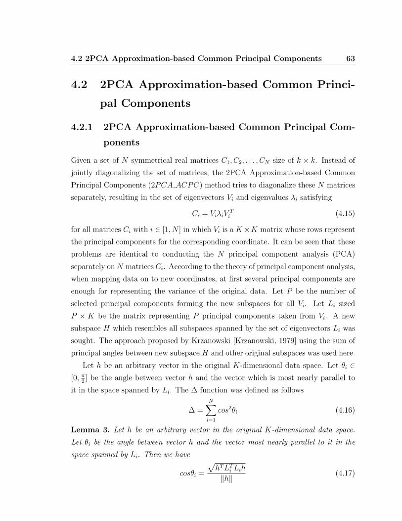
4.2 2PCA Approximation-based Common Principal Components 63
4.2 2PCA Approximation-based Common Princi-
pal Components
4.2.1 2PCA Approximation-based Common Principal Com-
ponents
Given a set of N symmetrical real matrices C1, C2, . . . , CN size of k × k. Instead of
jointly diagonalizing the set of matrices, the 2PCA Approximation-based Common
Principal Components (2PCA ACPC) method tries to diagonalize these N matrices
separately, resulting in the set of eigenvectors Vi and eigenvalues λi satisfying
Ci = ViλiVTi (4.15)
for all matrices Ci with i ∈ [1, N ] in which Vi is a K×K matrix whose rows represent
the principal components for the corresponding coordinate. It can be seen that these
problems are identical to conducting the N principal component analysis (PCA)
separately onN matrices Ci. According to the theory of principal component analysis,
when mapping data on to new coordinates, at first several principal components are
enough for representing the variance of the original data. Let P be the number of
selected principal components forming the new subspaces for all Vi. Let Li sized
P × K be the matrix representing P principal components taken from Vi. A new
subspace H which resembles all subspaces spanned by the set of eigenvectors Li was
sought. The approach proposed by Krzanowski [Krzanowski, 1979] using the sum of
principal angles between new subspace H and other original subspaces was used here.
Let h be an arbitrary vector in the original K-dimensional data space. Let θi ∈[0, π
2] be the angle between vector h and the vector which is most nearly parallel to
it in the space spanned by Li. The ∆ function was defined as follows
∆ =N∑i=1
cos2θi (4.16)
Lemma 3. Let h be an arbitrary vector in the original K-dimensional data space.
Let θi be the angle between vector h and the vector most nearly parallel to it in the
space spanned by Li. Then we have
cosθi =
√hTLTi Lih
‖h‖(4.17)

4.2 2PCA Approximation-based Common Principal Components 64
Proof. It can be seen that by the definition, the angle θi is the angle between vector h
and its project on the subspace spanned by Li. Let p be the project of h on subspace
spanned by Li. Due to the fact that Li is the basic of the subspace the vector p can
be rewritten as
p = LTi x (4.18)
The projected vector of h on the subspace perpendicular to subspace spanned by Li
is h− LTi x. Therefore,
Li(h− LTi x) = 0 (4.19)
Lih− LiLTi x = 0 (4.20)
x = (LiLTi )−1Lih (4.21)
Substitute (4.21) to (4.18), we have
p = LTi (LiLTi )−1Lh (4.22)
The orthogonality of Li gives us
p = LTi Lih (4.23)
The cosine of angle between the two vectors by definition is
cos(θi) =hTLTi Lih
‖hT‖‖LTi Lih‖(4.24)
Rewriting the norm of vector in dot product operator leads to
‖LTi Lih‖ =
√(LTi Lih)
T(LTi Lih) (4.25)
=√hTLTi LiL
Ti Lih (4.26)
=√hTLTi Lih (4.27)
Substitute (4.27) to (4.24), (4.17) is achieved. The theorem is proven.
Lemma 4. Let h be an arbitrary vector in the original K-dimensional data space.
Let θi be the angle between vector h and the vector most nearly parallel to it in the
space spanned by Li. Then the value of h is given by the eigenvector h1 corresponding
to the largest eigenvalue λ1 of the matrix L =∑
LTi Liwill maximize the value of ∆.

4.2 2PCA Approximation-based Common Principal Components 65
Proof. According to Lemma (3), we have
∆ =N∑i=1
cos2θi =hTLTi Lih
‖h‖2(4.28)
=hT∑N
i=1(LTi Li)h
hTh(4.29)
=hTLh
hTh(4.30)
The original optimal problem of finding arbitrary vector h that maxhhTLhhT h
is then con-
verted to the simpler optimal problem of finding normal vector h that max‖h‖=1hTLh.
Let V be the matrix used for diagonalizing matrix L as follows
L = V DV T (4.31)
in which
D = diag(λ1, λ2, , λn) (4.32)
and
λ1 ≥ λ2 ≥ · · · ≥ λn (4.33)
It will be proved that sup‖h‖=1hTL ≤ λ1. Let y = V Th. That ‖h‖ = 1 leads
to ‖y‖ = 1. Then max‖h‖=1hTLh = max‖y‖=1y
TDy = max‖y‖=1
∑Ki=1 λi‖yi‖
2 ≤max‖y‖=1
∑Ki=1 λ1‖yi‖
2 = λ1. The equality happens only when vector h is h1 which
is an eigenvector of the unit norm associated with the largest eigenvalue λ1. The
theorem is proven.
Applying the Gram-Schmidt method, it is seen that the eigenvector h2 associated
to the second largest eigenvalue of matrix D will be orthogonal to vector h1, which
leads to the second largest value of ∆. Similarly, the remaining K vectors hi which
will span the new subspace H was formed. Moreover, it can be seen that finding the
new subspace H is actually to conduct another Principal Component Analysis on the
matrix L. Therefore Q components from K components of subspace H can then be
selected, which are enough to represent all data points.
Algorithm 2 shows the pseudo code of the algorithm in finding common principal
components by using two times of principal component analysis.
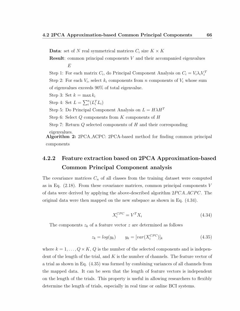
4.2 2PCA Approximation-based Common Principal Components 66
Data: set of N real symmetrical matrices Ci size K ×KResult: common principal components V and their accompanied eigenvalues
E
Step 1: For each matrix Ci, do Principal Component Analysis on Ci = ViλiVTi
Step 2: For each Vi, select ki components from n components of Vi whose sum
of eigenvalues exceeds 90% of total eigenvalue.
Step 3: Set k = max ki
Step 4: Set L =∑n
i (LTi Li)
Step 5: Do Principal Component Analysis on L = HλHT
Step 6: Select Q components from K components of H
Step 7: Return Q selected components of H and their corresponding
eigenvalues.Algorithm 2: 2PCA ACPC: 2PCA-based method for finding common principal
components
4.2.2 Feature extraction based on 2PCA Approximation-based
Common Principal Component analysis
The covariance matrices Cn of all classes from the training dataset were computed
as in Eq. (2.18). From these covariance matrices, common principal components V
of data were derived by applying the above-described algorithm 2PCA ACPC. The
original data were then mapped on the new subspace as shown in Eq. (4.34).
XCPCi = V TXi (4.34)
The components zk of a feature vector z are determined as follows
zk = log(yk) yk = [var(XCPCi )]k (4.35)
where k = 1, . . . , Q×K, Q is the number of the selected components and is indepen-
dent of the length of the trial, and K is the number of channels. The feature vector of
a trial as shown in Eq. (4.35) was formed by combining variances of all channels from
the mapped data. It can be seen that the length of feature vectors is independent
on the length of the trials. This property is useful in allowing researchers to flexibly
determine the length of trials, especially in real time or online BCI systems.

4.2 2PCA Approximation-based Common Principal Components 67
Due to the orthogonal property of new subspace, data on common principal com-
ponents are de-correlated. Moreover, eigenvalues represent the variance degree of
corresponding principal components. The feature vector of a trial as shown in Eq.
(4.35) was formed by combining the variances of all channels from the mapped data.
To remove the nonlinear property of variances, logarithm function was then applied.

Chapter 5
Experiments with
Approximation-based Common
Principal Component Analysis
This chapter presents the experiments undertaken with ACPC methods proposed
in the previous chapter. The dataset 2a of the BCI competition IV was used in
the experiments. The chapter starts with the description of the dataset used in
the experiments. It then follows with experimental methods and results. Using the
popular dataset in MBCI systems, it was proven that the proposed ACPC methods
enhanced the performance of the MBCI system. The last section contains discussions
about the experimental results and the effects of the relevant parameters on the
classification accuracy.
5.1 Dataset used in experiments
The Dataset 2a from the BCI Competition IV [Brunner et al., 2008], which is a well-
known dataset for multi-class BCI systems, is chosen for conducting experiments.
The dataset was acquired by Graz University of Technology, Austria using Electroen-
cephalography (EEG) technology with 22 channels at sampling frequency 250Hz. It
was then bandpass-filtered with the low and high cut-off frequencies at 0.5Hz and
100Hz, respectively. Another 50Hz notch filter was also applied to eliminate power
69

5.1 Dataset used in experiments 70
line noise. Nine subjects were asked to perform four classes of motor imagery tasks
to move cursor left, right, down or up corresponding with the imagination of move-
ment of the left hand, right hand, both feet and tongue. Each subject participated
in two sessions in different days. In each session, there were six runs separated by
short breaks in between. There were forty eight trials in each run which were equally
distributed for all the four classes. In total, there were 288 per sessions and 576 trials
per subject. For each trial, there were two seconds to help the participants prepare
themselves. After that, there was a cue appearing and staying on screen in 1.25s.
The subjects were asked to carry out motor imagery tasks until the 6th second. The
paradigm of getting this dataset is illustrated in Fig. 5.1. Fig. 5.2 shows the positions
of electrode used in the experiment corresponding to the standard 10-20 international
system. Distance between two neighbour electrodes is 3.5 centimetres.
Figure 5.1: Timing scheme of a run used in getting the dataset 2a of the BCI Com-
petition IV (extracted from [Brunner et al., 2008])
The dataset was used in the BCI Competition IV in 2008 and became a standard
dataset for multi-class BCI systems. In the competition, trials conducted by a subject
were equally divided into training and testing sets. The competitors were asked to
continuously assign labels to segments extracted from unknown trials. The winner
was the one who could achieve the largest kappa coefficient [Schlogl et al., 2007] cor-
responding to the highest accuracy at any time point. In the research’s experiments,
accuracy was used as the measurement, leading to the conversion of the results in
the competition [Brunner et al., 2008] which is reported by Kappa coefficient to the
classification accuracy using the equation accuracy = N×κ−κ+1N
proposed in [Schlogl
et al., 2007], wherein N = 4 and κ is the Kappa coefficient. Table 5.1 shows the re-
sults of five participants in the competition on the dataset 2a. It is noted that while

5.1 Dataset used in experiments 71
Figure 5.2: The electrode positions corresponding to the 10-20 international system
used in getting the dataset 2a of the BCI Competition IV (extracted from [Brunner
et al., 2008])

5.2 Experiment methods and validations 72
Table 5.1: The classification results (accuracy in percentage) on Dataset 2a of nine
subjects of the participating competitors in the BCI Competition IV [BCI, 2008]. The
results were converted from Kappa coefficient to accuracy measure (in percentage)
and rounded to the nearest integer values.
Author S1 S2 S3 S4 S5 S6 S7 S8 S9
Kai Keng Ang 76 57 81 61 55 45 83 81 71
Liu Guangquan 77 51 78 58 37 41 75 80 77
Wei Song 54 39 61 50 30 36 47 62 58
Damien Coyle 60 44 74 48 34 30 25 60 57
Jin Wu 56 38 54 44 30 37 51 59 53
using the dataset and its protocol in following experiments, the research’s purpose
was not to compete with other competitors in the competition. Instead, the dataset
was used to illustrate and test the proposed methods with the current state-of-the-art
methods which are based on CSP analysis.
5.2 Experiment methods and validations
The main purpose is to compare the proposed ACPC methods, Jacobi ACPC and
2PCA ACPC in multi-class BCI systems with two other popular CSP -based meth-
ods (CSP 1vsN and CSP pairs) and with another method based on individual chan-
nel TDP . These base-line methods are presented in Chapter 3. The Dataset 2a from
BCI Competition IV [BCI, 2008] which is described above was used for conducting
experiments.
As in the competition, data was segmented into lengths of 2 seconds from the
time point 2.5 second. Segment window was moved by one half of a second time
frame. All these segments were bandpass filtered with the frequency cut-off at 8Hz
and 30Hz before being extracted features depending on the methods used. Support
Vector Machine (SVM) and its popular kernel function RBF K(x, x′) = e−γ‖x−x′‖2 , a
state of the art method for classifying in BCI systems [Lotte et al., 2007], was chosen
5.3 Experimental results 73
to classify data. Grid search was applied to get the optimal classifiers. The parameter
γ was searched in the range {2k : k = −10,−9, . . . , 19, 20}. The trade-off parameter
C was searched over the grid {2k : k = 0, 1, . . . , 12, 13}.To evaluate the accuracy of classification on the dataset, the segmented data was
divided into training and testing data sets by ratio of 8:2. The testing data was
normalized basing on the distribution parameters extracted from the training data
set. A 5-fold cross validation test was performed on the training data to find the
optimal parameters γ and C. These optimal parameters were then used to build
classifiers for the entire training dataset. Finally, the classifiers were applied on the
testing dataset to get the accuracy results. To reduce randomness due to the division
of data into the training and testing sets, this process was run five times. The reported
accuracy results were calculated by taking the average of the accuracies of the results
for five runs.
5.3 Experimental results
Two main experiments were conducted. In the first experiment, the research’s purpose
was to compare the proposed methods Jacobi ACPC and 2PCA ACPC with CSP -
based methods including CSP 1vsN and CSP pairs on the chosen dataset. In the
second experiment, multi-channel based feature extraction methods were compared
with a typical single channel based feature extraction method named Time Domain
Parameters. Several other experiments were conducted to see the effects of selected
parameters on performance of Jacobi ACPC and 2PCA ACPC and visualization.
Although it was not aimed to compare with participants of the BCI Competition IV
on the same dataset, results of the proposed ACPC methods and theirs were briefly
analyzed. These experiments and their results are presented in section 5.4.
In the two main experiments, seventeen components which contribute about 80%
of the sum of eigenvalues of all components for 2PCA ACPC were selected. To
make it comparable with 2PCA ACPC, sixteen components for Jacobi ACPC were
selected. For the other CSP-based methods, as in other work, two components were
selected for each class for each CSP problem. Therefore, for the one-versus-the-rest
CSP, its feature vector has size 4 × 2 × n = 8 × n while for the pair-wise CSP, its
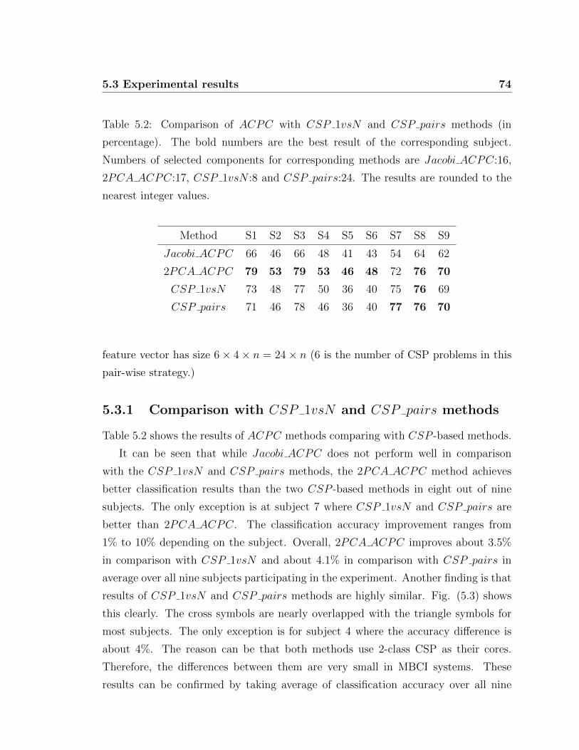
5.3 Experimental results 74
Table 5.2: Comparison of ACPC with CSP 1vsN and CSP pairs methods (in
percentage). The bold numbers are the best result of the corresponding subject.
Numbers of selected components for corresponding methods are Jacobi ACPC:16,
2PCA ACPC:17, CSP 1vsN :8 and CSP pairs:24. The results are rounded to the
nearest integer values.
Method S1 S2 S3 S4 S5 S6 S7 S8 S9
Jacobi ACPC 66 46 66 48 41 43 54 64 62
2PCA ACPC 79 53 79 53 46 48 72 76 70
CSP 1vsN 73 48 77 50 36 40 75 76 69
CSP pairs 71 46 78 46 36 40 77 76 70
feature vector has size 6× 4× n = 24× n (6 is the number of CSP problems in this
pair-wise strategy.)
5.3.1 Comparison with CSP 1vsN and CSP pairs methods
Table 5.2 shows the results of ACPC methods comparing with CSP -based methods.
It can be seen that while Jacobi ACPC does not perform well in comparison
with the CSP 1vsN and CSP pairs methods, the 2PCA ACPC method achieves
better classification results than the two CSP -based methods in eight out of nine
subjects. The only exception is at subject 7 where CSP 1vsN and CSP pairs are
better than 2PCA ACPC. The classification accuracy improvement ranges from
1% to 10% depending on the subject. Overall, 2PCA ACPC improves about 3.5%
in comparison with CSP 1vsN and about 4.1% in comparison with CSP pairs in
average over all nine subjects participating in the experiment. Another finding is that
results of CSP 1vsN and CSP pairs methods are highly similar. Fig. (5.3) shows
this clearly. The cross symbols are nearly overlapped with the triangle symbols for
most subjects. The only exception is for subject 4 where the accuracy difference is
about 4%. The reason can be that both methods use 2-class CSP as their cores.
Therefore, the differences between them are very small in MBCI systems. These
results can be confirmed by taking average of classification accuracy over all nine
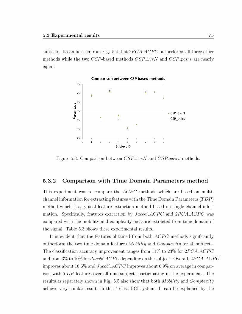
5.3 Experimental results 75
subjects. It can be seen from Fig. 5.4 that 2PCA ACPC outperforms all three other
methods while the two CSP -based methods CSP 1vsN and CSP pairs are nearly
equal.
Figure 5.3: Comparison between CSP 1vsN and CSP pairs methods.
5.3.2 Comparison with Time Domain Parameters method
This experiment was to compare the ACPC methods which are based on multi-
channel information for extracting features with the Time Domain Parameters (TDP )
method which is a typical feature extraction method based on single channel infor-
mation. Specifically, features extraction by Jacobi ACPC and 2PCA ACPC was
compared with the mobility and complexity measure extracted from time domain of
the signal. Table 5.3 shows these experimental results.
It is evident that the features obtained from both ACPC methods significantly
outperform the two time domain features Mobility and Complexity for all subjects.
The classification accuracy improvement ranges from 11% to 23% for 2PCA ACPC
and from 3% to 10% for Jacobi ACPC depending on the subject. Overall, 2PCA ACPC
improves about 16.6% and Jacobi ACPC improves about 6.9% on average in compar-
ison with TDP features over all nine subjects participating in the experiment. The
results as separately shown in Fig. 5.5 also show that both Mobility and Complexity
achieve very similar results in this 4-class BCI system. It can be explained by the

5.3 Experimental results 76
Figure 5.4: Ranking of ACPC and CSP methods based on classification accuracy
average over all nine subjects.
Table 5.3: Comparison of ACPC with Time Domain Parameters feature (in per-
centage). The bold numbers are the best result of the corresponding subject. The
number of selected components for the corresponding methods are Jacobi ACPC:16
and 2PCA ACPC:17. The results are rounded to the nearest integer values.
Method S1 S2 S3 S4 S5 S6 S7 S8 S9
Jacobi ACPC 66 46 66 48 41 43 54 64 62
2PCA ACPC 79 53 79 53 46 48 72 76 70
Mobility 56 39 60 42 31 36 49 60 53
Complexity 57 38 60 43 31 36 49 61 53

5.3 Experimental results 77
fact that in MBCI systems, interactions and variations among channels becomes more
complexity such that the Mobility and Complexity measures which are based on sin-
gle channel information seem to have reached their limit. These results can be con-
firmed by taking average of classification accuracy over all nine subjects. It can be
seen from Fig. 5.6 that 2PCA ACPC and Jacobi ACPC are higher than the results
for the two TDP features while the results for the two TDP features Mobility and
Complexity are nearly equal.
Figure 5.5: Comparison between Mobility and Complexity features.
Figure 5.6: Ranking of ACPC methods and TDP features based on classification
accuracy average over all nine subjects.
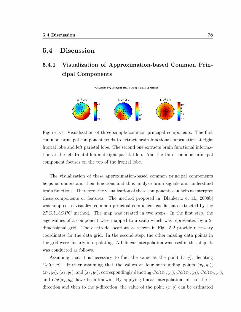
5.4 Discussion 78
5.4 Discussion
5.4.1 Visualization of Approximation-based Common Prin-
cipal Components
Figure 5.7: Visualization of three sample common principal components. The first
common principal component tends to extract brain functional information at right
frontal lobe and left parietal lobe. The second one extracts brain functional informa-
tion at the left frontal lob and right parietal lob. And the third common principal
component focuses on the top of the frontal lobe.
The visualization of these approximation-based common principal components
helps us understand their functions and thus analyze brain signals and understand
brain functions. Therefore, the visualization of these components can help us interpret
these components or features. The method proposed in [Blankertz et al., 2008b]
was adopted to visualize common principal component coefficients extracted by the
2PCA ACPC method. The map was created in two steps. In the first step, the
eigenvalues of a component were mapped to a scalp which was represented by a 2-
dimensional grid. The electrode locations as shown in Fig. 5.2 provide necessary
coordinates for the data grid. In the second step, the other missing data points in
the grid were linearly interpolating. A bilinear interpolation was used in this step. It
was conducted as follows.
Assuming that it is necessary to find the value at the point (x, y), denoting
Col(x, y). Further assuming that the values at four surrounding points (x1, y1),
(x1, y2), (x2, y1), and (x2, y2), correspondingly denoting Col(x1, y1), Col(x1, y2), Col(x2, y1),
and Col(x2, y2) have been known. By applying linear interpolation first to the x-
direction and then to the y-direction, the value of the point (x, y) can be estimated
5.4 Discussion 79
by Eq. (5.1).
Col(x, y) ≈ 1
(x2 − x1)(y2 − y1)(Col(x1, y1)(x2 − x)(y2 − y)
+Col(x2, y1)(x− x1)(y2 − y)
+Col(x1, y2)(x2 − x)(y − y1)
+Col(x2, y2)(x− x1)(y − y1))
(5.1)
Fig. 5.7 shows three sample common principal components formed by 2PCA ACPC
which have the largest corresponding eigenvalues. It is seen that different common
principal components target at different regions for spatial filtering. The first com-
mon principal component tends to extract brain functional information at the right
frontal lobe and left parietal lobe. The second one extracts brain functional informa-
tion at the left frontal lob and right parietal lob. And the third common principal
component focuses on the top of the frontal lobe. The visualizations of these com-
mon principal components also show that the CPCs are orthogonal. It means that
the most useful information extracted through these components is not overlapped.
Such visualizations can be useful for understanding brain functions in neutral related
disciplines .
5.4.2 Effect of the number of selected common principal com-
ponents on classification accuracy of 2PCA ACPC
As stated at the beginning of Section 5.3, 17 components which contribute about 80%
of sum of eigenvalues of all components for 2PCA ACPC were selected. It is seen
that the parameter of number of selected components is the most important one in
the 2PCA ACPC method. This experiment was designed to analyze the effects of
this important parameter on classification accuracy. The same dataset as in above
experiments was used for analysis. However, instead of selecting fixedly 80% of all
components, the number of selected components was varied. This variation could help
the research see the effect of number of selected components on classification accuracy.
Basically, the more number of selected components, the more information there was.
However, the more number of selected components, the more time was needed for

5.4 Discussion 80
training and testing the classifiers. The percentage of the sum of eigenvalues varied
from 20% to 100% with a step of 20%. Fig. 5.8 shows the classification accuracy of
the experiments.
Figure 5.8: The effect of the number of selected components on classification accuracy
of 2PCA ACPC method. The percentage numbers near the term 2PCA ACPC
are percentages of the sum of eigenvalues of all components to which the selected
components need to exceed.
The result shows that the number of selected components and the classification
accuracy have a positively linear relation. Moreover, in comparison with CSP-based
methods as shown in Fig. 5.9, even with 60% of the sum of eigenvalues, 2PCA ACPC
can achieve better accuracy than CSP 1vsN and CSP pairs for five subjects (S1, S2,
S4, S5, and S6), and slightly lower than or comparable to for other three subjects (S3,
S8, and S9) among all nine subjects. Similar comparison with TDP features shows
that even with 40% of the sum of eigenvalues 2PCA ACPC can achieve better accu-
racy than Mobility and Complexity features at all nine subjects. At the same time,
when the number of components was selected basing on 20% of the sum of eigen-
values, 2PCA ACPC can achieve better accuracy than Mobility and Complexity
for five subjects (S1, S4, S5, S6 and S9) among nine subjects participating in the
experiment. The results can be seen in Fig. 5.10.

5.4 Discussion 81
Figure 5.9: The effect of the number of selected components on classification accuracy
of 2PCA ACPC method when compared with CSP -based methods. The percentage
numbers near the term 2PCA ACPC are percentages of the sum of eigenvalues of
all components to which the selected components need to exceed.
Figure 5.10: The effect of the number of selected components on classification accu-
racy of 2PCA ACPC method when compared with TDP features. The percentage
numbers near the term 2PCA ACPC are percentages of the sum of eigenvalues of
all components to which the selected components need to exceed.

5.4 Discussion 82
5.4.3 Effect of the number of selected common principal com-
ponents on classification accuracy of Jacobi ACPC
As stated at the beginning of Section 5.3, 16 components were selected for Jacobi ACPC
analysis to make it comparable with 2PCA ACPC. This experiment was designed
to analyze the effects of the number of selected components on the classification ac-
curacy of Jacobi ACPC. Similarly to analyzing the effect of the number of selected
common principal components on classification of 2PCA ACPC, the same dataset
was used for analysis as in above experiments. The number of selected components
varied from 4 to 22 components with a step of 2. Fig. (5.11) shows classification
accuracy of the experiment.
Figure 5.11: The effect of the number of selected components on the classification
accuracy of Jacobi ACPC method. The numbers near the term Jacobi ACPC rep-
resent the number of selected components.
It is seen that, by trend, there is also a positively linear relation between the num-
ber of selected components and the classification accuracy when using Jacobi ACPC.
However, the trend is less stable than that of the 2PCA ACPC method. There are
some classification accuracy declines when number of selected components increases
in all nine subjects’ trend lines. In comparison with CSP -based base-line methods,
the classification accuracies are still lower than results of CSP 1vsN and CSP pairs

5.4 Discussion 83
for six subjects out of nine subjects (S1, S2, S3, S7, S8, and S9), although selecting all
22 components can help Jacobi ACPC achieve higher classification accuracy. For the
other three subjects, Jacobi ACPC achieves slightly better results than those of the
CSP -based methods. Meanwhile, in comparison with TDP features, Jacobi ACPC
is seen to achieve higher accuracy than or be comparable with TDP features when
experimented on 12 selected components. These results are shown in Fig. 5.12 and
Fig. 5.13.
Figure 5.12: The effect of the number of selected components on the classification
accuracy of Jacobi ACPC method when compared with CSP -based methods. The
numbers near the term Jacobi ACPC represent the number of selected components.
5.4.4 Comparison with participants of BCI Competition IV
on Dataset 2a
Although comparing with the participants of the BCI Compettion IV on the same
dataset was not the research’s purpose, this section presents a brief comparison be-
tween results of ACPC methods and of participants in the competition, due to work-
ing on the same dataset.
There were five competitors in the task on Dataset 2a of BCI Competition IV.
All of them used Common Spatial Patterns [BCI, 2008] as features in their models.
Kai et al. used the method applying CSP with One-versus-The-Rest strategy. More-

5.4 Discussion 84
Figure 5.13: The effect of the number of selected components on the classification
accuracy of Jacobi ACPC method when compared with TDP features. The numbers
near the term Jacobi ACPC represent the number of selected components.
over, their algorithm was based on the subject specific frequency band and heavily
depended on the feature selection technique called Mutual Information Best Individ-
ual Features. Liu applied the strategy of converting a multi-class BCI problem to
multiple 2-class BCI problems. The method has an adaptive window time selection.
Unfortunately, the authors did not explain much about this important step. The
three other groups of participants applied pure One-versus-The-Rest strategy and
did not rely on the feature selection method. These are the same as the proposed
ACPC methods so comparing with them is more appropriate. To compare on the
same measurement, the results in the competition [BCI, 2008] which is reported by
Kappa coefficient were converted to classification accuracy as proposed in [Schlogl
et al., 2007]. It is noted that the final results from the competition are actually the
maximum accuracy that a method could achieve, while the research’s results are the
averaged accuracies. Table 5.4 shows these results.
In general, 2PCA ACPC is the best for the first six subjects, the second place
for subjects S8 and S9, and the third place for subject S7. Meanwhile, the other
method, Jacobi ACPC, has higher accuracy than those of Wei, Damien, and Jin and
lower than those of Kai and Liu. In exceptional cases, Jacobi ACPC works well for
Subject 6 (the best) and for Subject 5 (the second) while it does not work well for

5.4 Discussion 85
Table 5.4: Comparison of classification accuracy between ACPC and methods of
the participants (in %) on Dataset 2a of BCI Competition IV. The results of the
competition are converted from Kappa coefficient to accuracy measure and rounded
to the nearest integer values. The results of 2PCA ACPC and Jacobi ACPC are
rounded to the nearest integer values. 2PCA ACPC and Jacobi ACPC use 22
components.
Author S1 S2 S3 S4 S5 S6 S7 S8 S9
Kai’s 76 57 81 61 55 45 83 81 71
Liu’s 77 51 78 58 37 41 75 80 77
Wei’s 54 39 61 50 30 36 47 62 58
Damien’s 60 44 74 48 34 30 25 60 57
Jin’s 56 38 54 44 30 37 51 59 53
Jacobi ACPC 70 46 71 50 48 50 55 66 64
2PCA ACPC 84 59 82 58 51 51 74 80 75
Subject 7. A close look at the detailed description of algorithms of five participated
groups shows that the proposed method Jacobi ACPC has higher accuracy than pure
One-versus-The-Rest strategy without any expensive feature selection mechanism and
has lower accuracy than the same strategy equipped with expensive feature selection
techniques. This result is confirmed by taking average of classification accuracy over
all nine subjects. On average, over all nine subjects, 2PCA ACPC is the best method
while Jacobi ACPC achieves higher classification accuracy than the methods used
by Wei, Damien and Jin. Fig. 5.14 shows this result.

5.4 Discussion 86
Figure 5.14: Comparison between the proposed ACPC methods with the methods
of the participants in the BCI Competition IV on Dataset 2a. The classification
accuracy is averaged over all nine subjects.

Chapter 6
General Aggregate Models for
Motor Imagery-Based BCI
Systems
This chapter investigates the effect of activation and delay issue in BCI experiments.
This effect leads to very high inter-session and inter-subject variability when conduct-
ing BCI experiments which complicates the analysis of BCI systems. Overcoming the
issue can enhance improvement of the BCI systems. Two general aggregate models
at score and feature levels were introduced here, to overcome the issue. The chapter
begins with an introduction to activation and delay issue in BCI experiments. It
then comes with the proposed general aggregate models. Experimental methods and
results of the proposed aggregate models are discussed in the following chapter.
6.1 Activation and delay issue in BCI experiments
The activation and delay issue is well known [Macaluso et al., 2007][Toni et al., 1999]
in conducting experiments in BCI systems. It is an effect in which the times of
stimulus and response, that are expected to be the same or nearly the same, are
actually different. In theory, when receiving stimulation input, the brain needs time
to process and then produce output. Macaluco et. al. in their work [Macaluso et al.,
2007], using fMRI in a delay paradigm, experimented with two sensory modalities:
87
6.2 Analysis on activation and delay issue using fNIRS 88
vision or touch, two motor effectors: eyes or hands, and two movements: left or
right. They found that there are delay activations which depending on subjects
and types of motor activity. Their work, however, mainly focuses on estimating
the delay which is the start time point but not the end time point which helps
extract the meaningful portion of the trial. This delay effect, in turn, is the origin
of the high inter-subject and inter-session variability which makes BCI systems very
difficult to become practical systems. Beside that, the experiments using functional
Near Infrared Spectroscopy (fNIRS) technology [Hoang et al., 2013a][Hoang et al.,
2013b], which will be presented in details in section 6.2, show that even within a
trial, subjects can lose their concentration; therefore, there are multiple portions
containing meaningful signal in a trial rather than one. Thus, the proposed method
is based on aggregate models instead of dealing directly with these issues.
Aggregate model is a well known approach in signal processing, especially in speech
signal processing [Ellis, 1997]. There are two main types of aggregate model. In the
first type, a trial is divided into multiple signal frames. Features of these frames are
then extracted and used for training classifiers. After that, the classification result of a
trial is determined by a aggregate function whose input are results from classifying its
frames. The aggregate function can be a min, max, average or count-based function.
In the second type, the aggregate model is called fusion model in which different
sources, features or classifiers of the same trial are combined by a aggregate function.
While the fusion model is widely used in BCI systems [Zhang et al., 2007][Gurkok
and Nijholt, 2012], there were a few work following the first type of aggregate models
which successfully applied to other signals such as speech.
6.2 An experimental analysis on activation and de-
lay issue using fNIRS
6.2.1 Subjects
Seven healthy subjects who were all male and within the age range from 20 to 31
voluntarily participated in the study. None of the recruited subjects had neurological
or psychiatric history or was on medication. Each of them gave written informed

6.2 Analysis on activation and delay issue using fNIRS 89
consent for the experiment. All experiments were performed at the Laboratory of
Biomedical Engineering Department of International University, Viet Nam. During
the experiment, the subjects sat on a comfortable arm-chair in a dark and sound
proof room.
6.2.2 Experimental procedure
All of the subjects were asked to sit on an arm-chair in front of a screen which
displayed the stimuli in a dark and sound proof room. Three protocols were used.
The first protocol (Fig. 6.1a) consisted of five loops including interchange of two left-
hand and two right-hand imagery loops. Each of these loops lasted 30 seconds. At
the end, there was a resting loop which lasted 10 seconds. In total, a trial lasted 130
seconds. The second protocol (Fig. 6.1b) (the third protocol Fig. 6.1b) consisted of
four loops including three left-hand imagery loops (right-hand correspondingly) and
a resting loop at final. Therefore, a trial of the second protocol lasted 100 seconds.
A typical loop as shown in Fig. 6.1d consisted of 10 seconds of resting and then 20
seconds of left or right imagery task. Three videos were designed following the three
above protocols. In these stimulated videos, there was a ball which moved to the left
or right, and rotated to the left or right corresponding to the stimuli. During the
resting time, a blank screen was displayed. In imagery time, the subjects clutched a
ball by their left hand or right hand corresponding to the stimuli on the screen. Every
subject was asked to finish all three protocols at one session. There were four subjects
taking part in experiments for one session, two subjects taking part in experiments
for two sessions, and one subject taking part in experiments for three sessions. The
variation in the number of sessions taken part in by the subjects was due to the
constraint of time. Any two different sessions of the same subject were conducted on
two different days.
6.2.3 Data acquisition
A 14-channel NIRS instrument (Shimadzu FOIRE3000) was used for acquiring oxy-
genated and deoxygenated haemoglobin concentration changes during the experi-
ments. It operated at three different wavelengths of 780 nm, 805 nm and 830 nm,

6.2 Analysis on activation and delay issue using fNIRS 90
(a) The first protocol with two left and right cues mixed together.
(b) The second protocol with three left cues.
(c) The third protocol with three right cues.
(d) A typical 30 second loop includes 10 seconds for resting and 20 seconds for specifical
cue (left or right).
Figure 6.1: Protocols were used in fNIRS experiments to prove activation and delay
issue.
emitting an average power of 3 mWmm−2. The detector optodes were placed at a
distance of 3 cm from the illuminator optodes. The optodes were arranged on the left
and right hemisphere of the subject’s head, above the motor cortex, around C3 (left
hemisphere) and C4 (right hemisphere) areas (according to the International 10-20
System) as illustrated in 6.2. For each hemisphere, three illuminators and three de-
tectors were used. A pair of illuminator and detector optodes formed one channel. So
in total, there were seven channels on each hemisphere, and fourteen channels on both
hemispheres. The photomultiplier cycled through all the illuminatordetector pairings
to acquire data at every sampling period. The sampling rate was approximately 18.2
Hz. Finally, the acquired signal was digitized by a 16bit analog to digital converter.
The used fNIRS imaging system adopted the near infrared lasers of three wave-
lengths: 780 nm, 805 nm, and 830 nm. For each channel j − th among fourteen
channels, optical densities Aj,λ at all wavelengths λ are measured. Then, from the
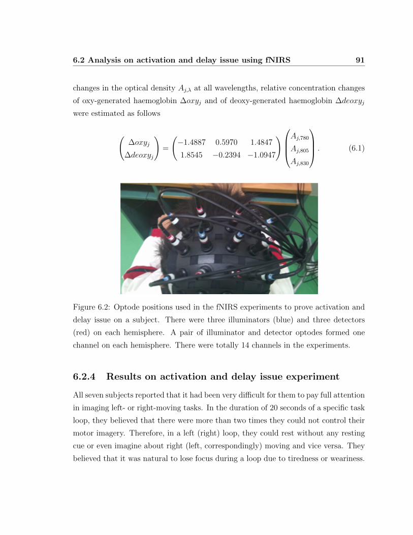
6.2 Analysis on activation and delay issue using fNIRS 91
changes in the optical density Aj,λ at all wavelengths, relative concentration changes
of oxy-generated haemoglobin ∆oxyj and of deoxy-generated haemoglobin ∆deoxyj
were estimated as follows
(∆oxyj
∆deoxyj
)=
(−1.4887 0.5970 1.4847
1.8545 −0.2394 −1.0947
)Aj,780
Aj,805
Aj,830
. (6.1)
Figure 6.2: Optode positions used in the fNIRS experiments to prove activation and
delay issue on a subject. There were three illuminators (blue) and three detectors
(red) on each hemisphere. A pair of illuminator and detector optodes formed one
channel on each hemisphere. There were totally 14 channels in the experiments.
6.2.4 Results on activation and delay issue experiment
All seven subjects reported that it had been very difficult for them to pay full attention
in imaging left- or right-moving tasks. In the duration of 20 seconds of a specific task
loop, they believed that there were more than two times they could not control their
motor imagery. Therefore, in a left (right) loop, they could rest without any resting
cue or even imagine about right (left, correspondingly) moving and vice versa. They
believed that it was natural to lose focus during a loop due to tiredness or weariness.
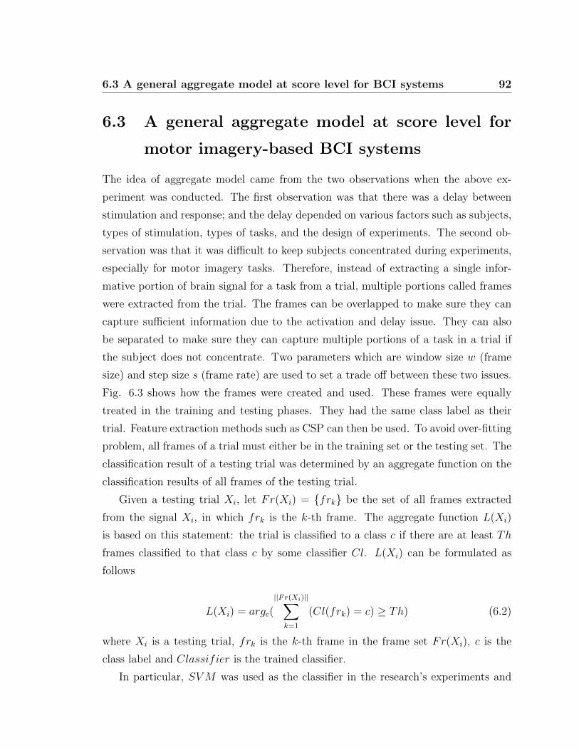
6.3 A general aggregate model at score level for BCI systems 92
6.3 A general aggregate model at score level for
motor imagery-based BCI systems
The idea of aggregate model came from the two observations when the above ex-
periment was conducted. The first observation was that there was a delay between
stimulation and response; and the delay depended on various factors such as subjects,
types of stimulation, types of tasks, and the design of experiments. The second ob-
servation was that it was difficult to keep subjects concentrated during experiments,
especially for motor imagery tasks. Therefore, instead of extracting a single infor-
mative portion of brain signal for a task from a trial, multiple portions called frames
were extracted from the trial. The frames can be overlapped to make sure they can
capture sufficient information due to the activation and delay issue. They can also
be separated to make sure they can capture multiple portions of a task in a trial if
the subject does not concentrate. Two parameters which are window size w (frame
size) and step size s (frame rate) are used to set a trade off between these two issues.
Fig. 6.3 shows how the frames were created and used. These frames were equally
treated in the training and testing phases. They had the same class label as their
trial. Feature extraction methods such as CSP can then be used. To avoid over-fitting
problem, all frames of a trial must either be in the training set or the testing set. The
classification result of a testing trial was determined by an aggregate function on the
classification results of all frames of the testing trial.
Given a testing trial Xi, let Fr(Xi) = {frk} be the set of all frames extracted
from the signal Xi, in which frk is the k-th frame. The aggregate function L(Xi)
is based on this statement: the trial is classified to a class c if there are at least Th
frames classified to that class c by some classifier Cl. L(Xi) can be formulated as
follows
L(Xi) = argc(
||Fr(Xi)||∑k=1
(Cl(frk) = c) ≥ Th) (6.2)
where Xi is a testing trial, frk is the k-th frame in the frame set Fr(Xi), c is the
class label and Classifier is the trained classifier.
In particular, SVM was used as the classifier in the research’s experiments and
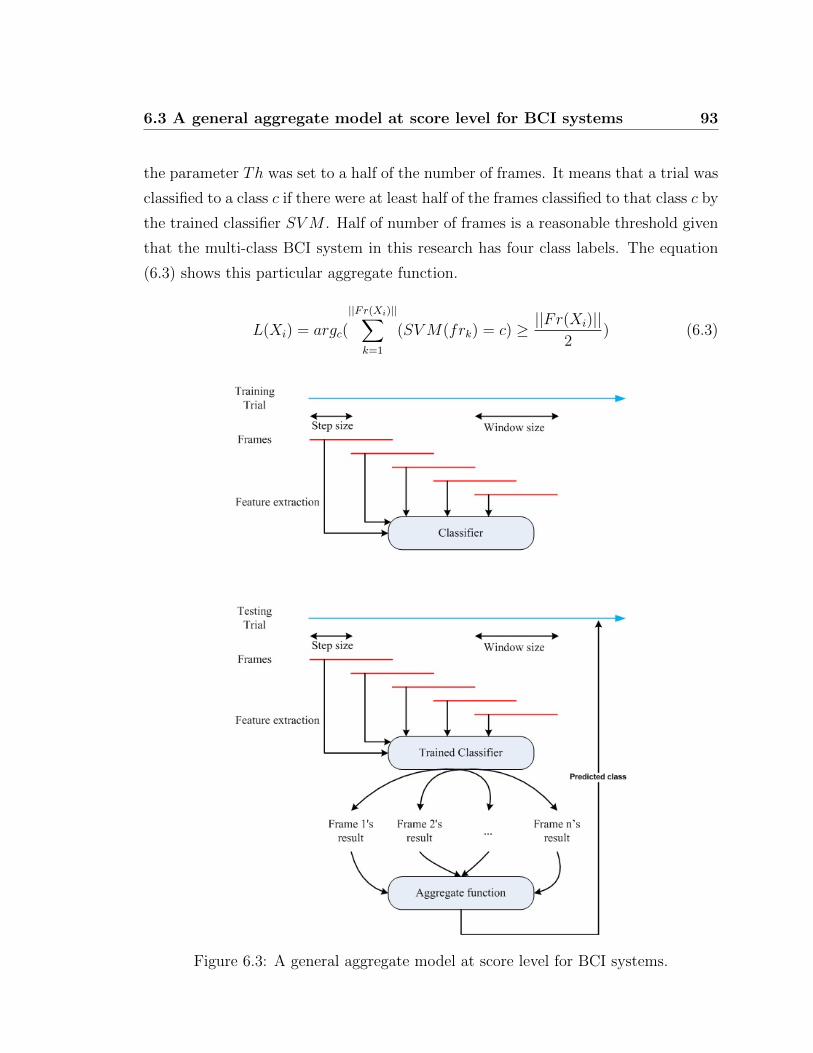
6.3 A general aggregate model at score level for BCI systems 93
the parameter Th was set to a half of the number of frames. It means that a trial was
classified to a class c if there were at least half of the frames classified to that class c by
the trained classifier SVM . Half of number of frames is a reasonable threshold given
that the multi-class BCI system in this research has four class labels. The equation
(6.3) shows this particular aggregate function.
L(Xi) = argc(
||Fr(Xi)||∑k=1
(SVM(frk) = c) ≥ ||Fr(Xi)||2
) (6.3)
Figure 6.3: A general aggregate model at score level for BCI systems.
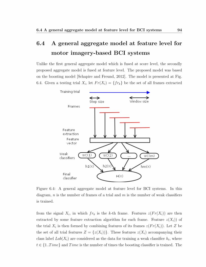
6.4 A general aggregate model at feature level for BCI systems 94
6.4 A general aggregate model at feature level for
motor imagery-based BCI systems
Unlike the first general aggregate model which is fused at score level, the secondly
proposed aggregate model is fused at feature level. The proposed model was based
on the boosting model [Schapire and Freund, 2012]. The model is presented at Fig.
6.4. Given a testing trial Xi, let Fr(Xi) = {frk} be the set of all frames extracted
Figure 6.4: A general aggregate model at feature level for BCI systems. In this
diagram, n is the number of frames of a trial and m is the number of weak classifiers
is trained.
from the signal Xi, in which frk is the k-th frame. Features z(Fr(Xi)) are then
extracted by some feature extraction algorithm for each frame. Feature z(Xi)) of
the trial Xi is then formed by combining features of its frames z(Fr(Xi)). Let Z be
the set of all trial features Z = {z(Xi))}. These features z(Xi) accompanying their
class label Lab(Xi) are considered as the data for training a weak classifier ht, where
t ∈ {1..T ime} and Time is the number of times the boosting classifier is trained. The
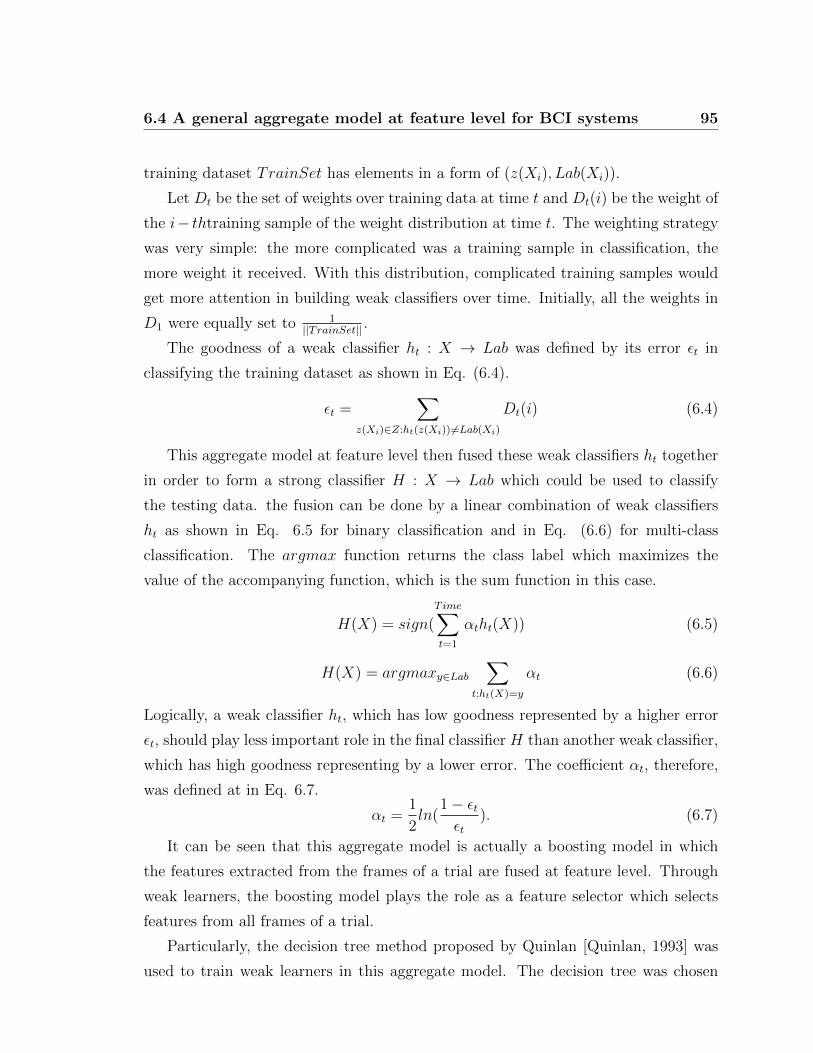
6.4 A general aggregate model at feature level for BCI systems 95
training dataset TrainSet has elements in a form of (z(Xi), Lab(Xi)).
Let Dt be the set of weights over training data at time t and Dt(i) be the weight of
the i− thtraining sample of the weight distribution at time t. The weighting strategy
was very simple: the more complicated was a training sample in classification, the
more weight it received. With this distribution, complicated training samples would
get more attention in building weak classifiers over time. Initially, all the weights in
D1 were equally set to 1||TrainSet|| .
The goodness of a weak classifier ht : X → Lab was defined by its error εt in
classifying the training dataset as shown in Eq. (6.4).
εt =∑
z(Xi)∈Z:ht(z(Xi)) 6=Lab(Xi)
Dt(i) (6.4)
This aggregate model at feature level then fused these weak classifiers ht together
in order to form a strong classifier H : X → Lab which could be used to classify
the testing data. the fusion can be done by a linear combination of weak classifiers
ht as shown in Eq. 6.5 for binary classification and in Eq. (6.6) for multi-class
classification. The argmax function returns the class label which maximizes the
value of the accompanying function, which is the sum function in this case.
H(X) = sign(T ime∑t=1
αtht(X)) (6.5)
H(X) = argmaxy∈Lab∑
t:ht(X)=y
αt (6.6)
Logically, a weak classifier ht, which has low goodness represented by a higher error
εt, should play less important role in the final classifier H than another weak classifier,
which has high goodness representing by a lower error. The coefficient αt, therefore,
was defined at in Eq. 6.7.
αt =1
2ln(
1− εtεt
). (6.7)
It can be seen that this aggregate model is actually a boosting model in which
the features extracted from the frames of a trial are fused at feature level. Through
weak learners, the boosting model plays the role as a feature selector which selects
features from all frames of a trial.
Particularly, the decision tree method proposed by Quinlan [Quinlan, 1993] was
used to train weak learners in this aggregate model. The decision tree was chosen

6.5 Segmented Spatial Filters for MBCI systems 96
because it is a lightweight classifier which is very efficient for being the weak classifiers
in the boosting model, and a multi-class oriented learning algorithm.
6.5 Segmented Spatial Filters for Multi-class Brain-
Computer Interface
As described above, the two general aggregate models are very flexible. In fact, they
can be used with any feature extraction including the CSP-based feature extrac-
tion methods and the research proposed ACPC analysis. This combination leads
to a new method called segmented spatial filters (SSF ). It inherits the advan-
tages from the both spatial filters such as ACPC and CSP -based methods, and
the aggregate models. As a result, The SSF method can not only improve the spa-
tial resolution of EEG signals but also efficiently deal with the inter-subject and
inter-session variability in BCI systems. Basing on this argument, six specific fea-
ture extraction models were proposed naming correspondingly SAM CSP 1vsN ,
SAM CSP pairs, SAM 2PCA ACPC, FAM CSP 1vsN , FAM CSP pairs and
FAM 2PCA ACPC. They were formed by combinations of CSP 1vsN , CSP pairs,
2PCA ACPC as feature extraction methods and the two general aggregate models
at score and feature levels. While the first three models were formed by using corre-
sponding feature extraction methods CSP 1vsN , CSP pairs and 2PCA ACPC in
the aggregate model at score level, the last three models were formed in the aggregate
model at feature level.
Taking into the view of aggregate model based on segments of trial instead of
the whole one, SAM 2PCA ACPC and SAM 2PCA ACPC are called segmented
approximation-based common principal components (SACPC) analysis. Similarly,
SAM CSP 1vsN , SAM CSP pairs, FAM CSP 1vsN , and FAM CSP pairs are
called segmented CSP-based feature method. Further taking into the fact that
the purpose of the three feature extraction methods CSP 1vsN , CSP pairs and
2PCA ACPC is to improve the spatial resolution of EEG signals, these six models
are called segmented spatial filters methods. These segmented spatial filters methods,
while still keep the property of improving the spatial resolution of brain signals, are
very robust when dealing with the inter-subject and inter-session variability in BCI

6.5 Segmented Spatial Filters for MBCI systems 97
experiments. In summary, they are expected to be efficient in both subject-dependent
multi-class and subject-independent multi-class BCI systems.

Chapter 7
Experiments with Aggregate
Models
This chapter presents the experiments undertaken with aggregate models proposed
in the previous chapter. The dataset 2a of the BCI competition IV was used in
the experiments. The spatial CSP -based feature extraction was used as the feature
extraction method in the aggregate models. Using the popular dataset in multi-
class multi-subject BCI systems, it was proven that the proposed aggregate models
enhanced the performance of both subject-dependent and subject-independent BCI
systems. The experimental results also showed that a combination of spatial filter
with segmented techniques in aggregate models is a very good solution in motor
imagery-based BCI systems.
7.1 Dataset used in experiments
As in experiments with the ACPC method, the Dataset 2a from the BCI Competition
IV [Brunner et al., 2008] which is a well-known dataset for multi-class BCI systems,
was chosen for conducting the experiments with the aggregate models. To make it
easier for readers to follow, a summary is provided here. For a detailed description,
readers should go to section 5.1.
The dataset was acquired by Graz University of Technology, Austria using Elec-
troencephalography (EEG) technology with 22 channels at sampling frequency 250Hz.
99
7.2 Experiment methods and validations 100
It was then bandpass-filtered with the low and high cut-off frequencies at 0.5Hz and
100Hz, respectively. Another 50Hz notch filter was also applied to eliminate power
line noise. Nine subjects were asked to perform 4 classes of motor imagery tasks by
moving cursor left, right, down or up corresponding with their imagination of move-
ment of the left hand, right hand, both feet and tongue. Each subject participated
in two sessions on two different days. In each session, there are six runs separated by
short breaks in between. There were forty eight trials in each run equally distributed
for all four classes. In total, there were 288 trials per session and 576 trials per subject.
For each trial, there were two seconds to help participants prepare themselves. After
that, there was a cue appearing and staying on screen in 1.25 seconds. The subjects
were asked to carry out motor imagery tasks until the 6th second. The paradigm of
getting this dataset is illustrated as in Fig. 5.1. Fig. 5.2 shows positions of the elec-
trodes used in the experiment and corresponding to the standard 10-20 international
system. The distance between the two neighbour electrodes is 3.5 centimetres.
7.2 Experiment methods and validations
The aim of the experiments was to evaluate and compare the proposed aggregate mod-
els with other non-aggregate models. Specifically, comparison was between CSP 1vsN ,
CSP pairs and 2PCA ACPC and their aggregate model versions respectively in-
cluding SAM CSP 1vsN , FAM CSP 1vsN , SAM CSP pairs, FAM CSP pairs,
SAM 2PCA ACPC, and FAM 2PCA ACPC as described in the previous chapter.
Being different from the experiments conducted with ACPC methods in which
the researcher used the similar processing and evaluation method to that proposed
by the competition organizers, a different processing and evaluation method was used
for the experiments reported with this chapter. In the ACPC experiments, as in the
competition proposed method, a real trial was divided into many pseudo-trials which
had 2-second lengths. In the aggregate model experiments, there was no pseudo-trial.
The real trial was treated as a whole one. Then, these proposed aggregate models
and base-line methods used the whole trial as their data for classification tasks.
As in the competition, the trial was extracted from the time point 2.5 second to
the end which was at the 6th second. The length of a trial was 3.5 seconds. All these
7.2 Experiment methods and validations 101
trials were bandpass filtered, with a frequency cut-off at 8Hz and 30Hz before be-
ing extracted features, depending on the methods being used. In the non-aggregate
models, features were extracted from the trial and then fed into a Support Vector
Machine (SVM) for the classification task. The SVM’s popular kernel function RBF
K(x, x′) = e−γ‖x−x′‖2 , a state of the art method for classifying in BCI systems [Lotte
et al., 2007], was chosen to classify the data. A grid search was applied to get the op-
timal classifiers. The parameter γ was searched in range 2k : k = −10,−9, . . . , 19, 20.
The trade-off parameter C was searched over the grid 2k : k = 0, 1, . . . , 12, 13. These
parameters are the same as in experiments of the ACPC analysis. SVM was also used
as classifiers in methods derived from the general aggregate model at score level. For
methods derived from the general aggregate model at feature level, the final strong
classifiers were used. In the boosting model, there is a parameter called numTree
to control the number of decision trees that can be used in the boosting algorithm.
Through the experiments, it was set to 200 decision trees. There was no additional
classifier used for these methods.
As stated in the previous chapter, aggregate models are expected to be robust,
not only in SD-BCI systems but also in SI-BCI systems. Therefore, there are two
main experiments reported in this chapter. The first experiment was about using
aggregate models in SD-BCI systems, while the second was about using aggregate
models in SI-BCI systems. In each of the main experiments, all six methods derived
from two general aggregate models, including SAM CSP 1vsN , SAM CSP pairs,
SAM 2PCA ACPC, FAM CSP 1vsN , FAM CSP pairs and FAM 2PCA ACPC,
were conducted and compared.
The validation method used in the experiments was the same as in the SD-BCI
experiments of the ACPC analysis. To evaluate the accuracy of the classification, the
dataset was divided into training and testing data sets by ratio of 8:2. This ratio of
training and testing data was fixed for both SI-BCI and SD-BCI experiments. More
specifically, in the SI-BCI experiments, data of all subjects were combined together
while in the SD-BCI experiments they were kept separately. The test data was
normalized based on distribution parameters extracted from the training data set. A
5-fold cross validation test on the training data was performed to find the optimal
parameters γ and C. These optimal parameters were then used to build classifiers
7.3 Experimental results 102
for the entire training dataset. Finally, the classifiers were applied on the testing
dataset to get accuracy results. To reduce randomness due to the division of data
into training and testing data, this process was run five times. The reported accuracy
results were calculated by taking the average of the accuracies of the results for five
runs.
7.3 Experimental results
7.3.1 Aggregate models in subject-dependent multi-class BCI
systems
As described in the experimental method section, the experiments in SD-BCI sys-
tems were conducted by training and testing classifiers for each subject separately.
The methods derived from aggregate models at score level (SAM) and feature level
(FAM) were compared with their corresponding non-aggregate model versions (NAM).
Specifically, SAM CSP 1vsN and FAM CSP 1vsN with CSP 1vsN ; SAM CSP pairs
and FAM CSP pairs with CSP pairs; and SAM 2PCA ACPC and FAM 2PCA ACPC
with 2PCA ACPC were compared. While non-aggregate methods including CSP 1vsN ,
CSP pairs and 2PCA ACPC were trained and tested on the whole trials, their ag-
gregate versions including SAM CSP 1vsN , SAM CSP pairs, SAM 2PCA ACPC,
FAM CSP 1vsN , FAM CSP pairs, and FAM 2PCA ACPC used segmented tri-
als with two parameters window size w and window step s, set to two seconds and half
of second respectively. Table 7.1 shows the classification results of the non-aggregate
methods. Note that 2PCA ACPC used the number of components corresponding to
80% of the sum of the eigenvalues of all components. The results of the comparison
between the non-aggregate methods and their aggregate models are presented in Figs.
7.1, 7.2 and 7.3.
It can be seen that in all three experiments, the aggregate models at score level
were better than, or at least equal to, their corresponding non-aggregate models for
most subjects. The accuracy improvement was at most at nearly 8.7% for SAM CSP 1vsN
method. There were three exceptional cases where non-aggregate methods defeated
their aggregate models at score level. The three cases were equally distributed for the
three methods. They were at subject 8 for CSP 1vsN , at subject 4 for CSP pairs
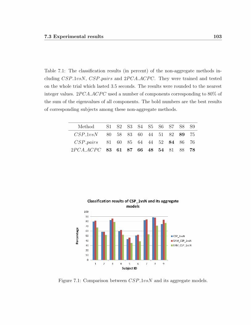
7.3 Experimental results 103
Table 7.1: The classification results (in percent) of the non-aggregate methods in-
cluding CSP 1vsN , CSP pairs and 2PCA ACPC. They were trained and tested
on the whole trial which lasted 3.5 seconds. The results were rounded to the nearest
integer values. 2PCA ACPC used a number of components corresponding to 80% of
the sum of the eigenvalues of all components. The bold numbers are the best results
of corresponding subjects among these non-aggregate methods.
Method S1 S2 S3 S4 S5 S6 S7 S8 S9
CSP 1vsN 80 58 83 60 44 51 82 89 75
CSP pairs 81 60 85 64 44 52 84 86 76
2PCA ACPC 83 61 87 66 48 54 81 88 78
Figure 7.1: Comparison between CSP 1vsN and its aggregate models.

7.3 Experimental results 104
Figure 7.2: Comparison between CSP pairs and its aggregate models.
Figure 7.3: Comparison between 2PCA ACPC and its aggregate models.

7.3 Experimental results 105
Table 7.2: The improvement of classification accuracy (in percent) of
SAM CSP 1vsN , SAM CSP pairs, and SAM 2PCA ACPC over their non-
aggregate methods. The positive numbers represent better results, whereas the neg-
ative numbers mean worse results. The results were rounded to two decimal places.
2PCA ACPC used the number of components corresponding to 80% of the sum of
the eigenvalues of all components.
Method S1 S2 S3 S4 S5 S6 S7 S8 S9
SAM CSP 1vsN 1.74 0 3.13 2.78 2.78 1.74 1.57 -0.52 8.70
SAM CSP pairs 2.61 6.61 1.39 -0.87 7.65 2.44 3.83 0.17 2.61
SAM 2PCA ACPC 1.22 -0.17 0.52 0.52 3.13 1.04 4.00 1.22 6.96
and at subject 2 for 2PCA ACPC. On average over all subjects, aggregate models at
score level of CSP 1vsN , CSP pairs and 2PCA ACPC improved about 2.4%, 2.9%
and 2.0% respectively over their original methods. Table 7.2 shows these results.
By comparison, aggregate models at feature level achieved significantly lower clas-
sification results than their non-aggregate methods. FAM CSP 1vsN , FAM CSP pairs,
and FAM 2PCA ACPC were only better than their non-aggregate methods at sub-
ject 9 as shown in Figs. 7.1, 7.2 and 7.3.
The improvement in classification accuracy of the proposed aggregate models at
score level leads to another question: whether or not the aggregate function is neces-
sary. This hypothesis was tested by leaving the framing technique and removing the
aggregate function. If this hypothesis was true, the length of trials in future exper-
iments could be significantly reduced. Unfortunately, experimental results as shown
in Figs. 7.4, 7.5 and 7.6 show that reducing the time for a trial will lead to a reduc-
tion of classification results for all these framing methods CSP 1vsN , CSP pairs and
2PCA ACPC compared with their non-framed models, which are also non-aggregate
models.
In conclusion for SD-BCI systems, compared with non-aggregate methods, the
corresponding aggregate models at score level improved classification accuracy up to
8.7% depending the subjects participating in the experiment in dataset 2a of the BCI

7.3 Experimental results 106
Figure 7.4: Comparison between CSP 1vsN and its framed version. The framed
version is the aggregate model without the aggregate function to combine results of
frames together.
Figure 7.5: Comparison between CSP pairs and its framed version. The framed
version is the aggregate model without the aggregate function to combine results of
frames together.
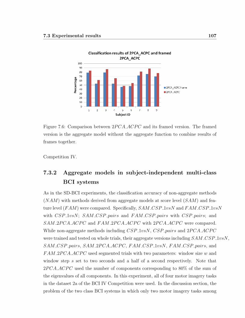
7.3 Experimental results 107
Figure 7.6: Comparison between 2PCA ACPC and its framed version. The framed
version is the aggregate model without the aggregate function to combine results of
frames together.
Competition IV.
7.3.2 Aggregate models in subject-independent multi-class
BCI systems
As in the SD-BCI experiments, the classification accuracy of non-aggregate methods
(NAM) with methods derived from aggregate models at score level (SAM) and fea-
ture level (FAM) were compared. Specifically, SAM CSP 1vsN and FAM CSP 1vsN
with CSP 1vsN ; SAM CSP pairs and FAM CSP pairs with CSP pairs; and
SAM 2PCA ACPC and FAM 2PCA ACPC with 2PCA ACPC were compared.
While non-aggregate methods including CSP 1vsN , CSP pairs and 2PCA ACPC
were trained and tested on whole trials, their aggregate versions including SAM CSP 1vsN ,
SAM CSP pairs, SAM 2PCA ACPC, FAM CSP 1vsN , FAM CSP pairs, and
FAM 2PCA ACPC used segmented trials with two parameters: window size w and
window step s set to two seconds and a half of a second respectively. Note that
2PCA ACPC used the number of components corresponding to 80% of the sum of
the eigenvalues of all components. In this experiment, all of four motor imagery tasks
in the dataset 2a of the BCI IV Competition were used. In the discussion section, the
problem of the two class BCI systems in which only two motor imagery tasks among

7.3 Experimental results 108
these four were used are discussed. The results of this experiment are shown in Fig.
7.7.
Figure 7.7: Comparison between CSP 1vsN , CSP pairs, 2PCA ACPC and their
corresponding aggregate models in a subject-independent multi-class BCI experiment.
NAM:Non-aggregate model; SAM:Aggregate model at score level; FAM:Aggregate
model at feature level. There were nine subjects in the experiment. 2PCA ACPC
used the number of components corresponding to 80% of the sum of the eigenvalues
of all components.
The results of this experiment are fairly consistent with the ones of the above
subject-dependent multi-class BCI. While the aggregate models at score level show
higher classification accuracy than their corresponding non-aggregate models, the ag-
gregate models at feature level show much lower classification accuracy. The best im-
provement in classification was of SAM 2PCA ACPC compared with its correspond-
ing non-aggregate model SAM 2PCA ACPC. It was about 4.77%. SAM CSP 1vsN
and SAM CSP pairs enhanced the classification accuray about 1.15% and 2.93%
over CSP 1vsN and CSP pairs, respectively.
Due to the property of high inter-subject variability of subject-independent multi-
class BCI systems, the experiment was extended by analysing different window step
s parameter values. Instead of only one value at one half seconds, the parameter
window step s value was now set to one second and one and a half seconds. Table
7.3 shows the best achieved results from variation of this parameter.

7.3 Experimental results 109
Figure 7.8: Multiple comparison test results of 4 models using CSP 1vsN methods
for 4-class SI-BCI systems. The non-aggregate model is represented by step size
s = 875. The step size 125, 250 and 375 correspond to duration of 0.5, 1 and 1,5
seconds.

7.3 Experimental results 110
Figure 7.9: Multiple comparison test results of 4 models using CSP pairs methods
for 4-class SI-BCI systems. The non-aggregate model is represented by step size
s = 875. The step size 125, 250 and 375 correspond to duration of 0.5, 1 and 1,5
seconds.

7.3 Experimental results 111
Figure 7.10: Multiple comparison test results of 4 models using 2PCA ACPC meth-
ods for 4-class SI-BCI systems. The non-aggregate model is represented by step size
s = 875. The step size 125, 250 and 375 correspond to duration of 0.5, 1 and 1,5
seconds.
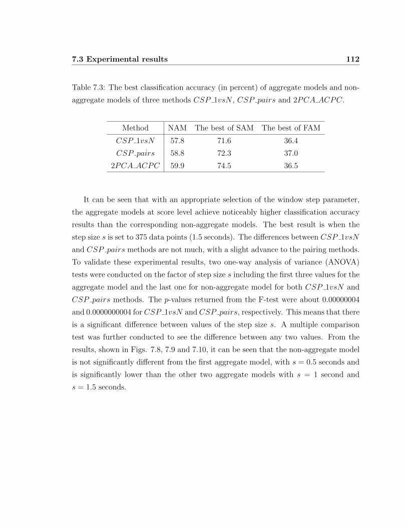
7.3 Experimental results 112
Table 7.3: The best classification accuracy (in percent) of aggregate models and non-
aggregate models of three methods CSP 1vsN , CSP pairs and 2PCA ACPC.
Method NAM The best of SAM The best of FAM
CSP 1vsN 57.8 71.6 36.4
CSP pairs 58.8 72.3 37.0
2PCA ACPC 59.9 74.5 36.5
It can be seen that with an appropriate selection of the window step parameter,
the aggregate models at score level achieve noticeably higher classification accuracy
results than the corresponding non-aggregate models. The best result is when the
step size s is set to 375 data points (1.5 seconds). The differences between CSP 1vsN
and CSP pairs methods are not much, with a slight advance to the pairing methods.
To validate these experimental results, two one-way analysis of variance (ANOVA)
tests were conducted on the factor of step size s including the first three values for the
aggregate model and the last one for non-aggregate model for both CSP 1vsN and
CSP pairs methods. The p-values returned from the F-test were about 0.00000004
and 0.0000000004 for CSP 1vsN and CSP pairs, respectively. This means that there
is a significant difference between values of the step size s. A multiple comparison
test was further conducted to see the difference between any two values. From the
results, shown in Figs. 7.8, 7.9 and 7.10, it can be seen that the non-aggregate model
is not significantly different from the first aggregate model, with s = 0.5 seconds and
is significantly lower than the other two aggregate models with s = 1 second and
s = 1.5 seconds.
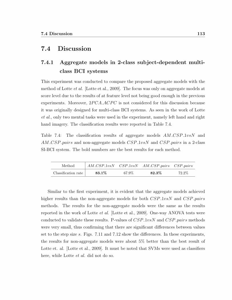
7.4 Discussion 113
7.4 Discussion
7.4.1 Aggregate models in 2-class subject-dependent multi-
class BCI systems
This experiment was conducted to compare the proposed aggregate models with the
method of Lotte et al. [Lotte et al., 2009]. The focus was only on aggregate models at
score level due to the results of at feature level not being good enough in the previous
experiments. Moreover, 2PCA ACPC is not considered for this discussion because
it was originally designed for multi-class BCI systems. As seen in the work of Lotte
et al., only two mental tasks were used in the experiment, namely left hand and right
hand imagery. The classification results were reported in Table 7.4.
Table 7.4: The classification results of aggregate models AM CSP 1vsN and
AM CSP pairs and non-aggregate models CSP 1vsN and CSP pairs in a 2-class
SI-BCI system. The bold numbers are the best results for each method.
Method AM CSP 1vsN CSP 1vsN AM CSP pairs CSP pairs
Classification rate 83.1% 67.9% 82.3% 72.2%
Similar to the first experiment, it is evident that the aggregate models achieved
higher results than the non-aggregate models for both CSP 1vsN and CSP pairs
methods. The results for the non-aggregate models were the same as the results
reported in the work of Lotte et al. [Lotte et al., 2009]. One-way ANOVA tests were
conducted to validate these results. P-values of CSP 1vsN and CSP pairs methods
were very small, thus confirming that there are significant differences between values
set to the step size s. Figs. 7.11 and 7.12 show the differences. In these experiments,
the results for non-aggregate models were about 5% better than the best result of
Lotte et. al. [Lotte et al., 2009]. It must be noted that SVMs were used as classifiers
here, while Lotte et al. did not do so.
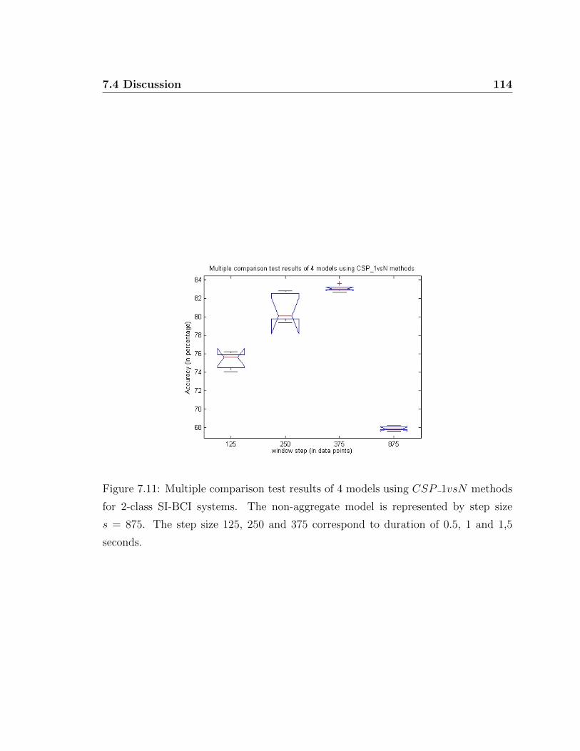
7.4 Discussion 114
Figure 7.11: Multiple comparison test results of 4 models using CSP 1vsN methods
for 2-class SI-BCI systems. The non-aggregate model is represented by step size
s = 875. The step size 125, 250 and 375 correspond to duration of 0.5, 1 and 1,5
seconds.

7.4 Discussion 115
Figure 7.12: Multiple comparison test results of 4 models using CSP pairs methods
for 2-class SI-BCI systems. The non-aggregate model is represented by step size
s = 875. The step size 125, 250 and 375 correspond to duration of 0.5, 1 and 1,5
seconds.

7.4 Discussion 116
7.4.2 SD-MBCI systems versus SI-MBC systems
This experiment was conducted for the purpose of finding the difference, if any, be-
tween SD-BCI and SI-BCI systems. In this experiment, the proposed aggregate mod-
els at score level were applied for both SD-BCI and SI-BCI systems. The focus was
on 4-class BCI systems. In SD-BCI systems, subjects were trained and tested indi-
vidually. The experimental method and validations for the SD-BCI experiments were
still the same as for the SI-BCI experiments except that the data of all subjects were
not mixed together. To compare the SD-BCI and SI-BCI systems, the results of the
SI-BCI were broken down by subject. All the results of the different values of the win-
dow step parameter s are presented here. The values used in this experiment included
0.5, 1 and 1.5 seconds which correspond to 125, 250 and 375 data points. The results
are reported in Tables 7.5, 7.6 and 7.7 which correspond with SAM CSP 1vsN ,
SAM CSP pairs and SAM 2PCA ACPC methods. To compare these classifica-
tion results, the accuracy differences, which is defined by subtracting the results of
SD-BCI from the corresponding results of SI-BCI, were calculated. Fig. 7.13, Fig.
7.14 and Fig. 7.15 show these differences for the SAM CSP 1vsN , SAM CSP pairs
and SAM 2PCA ACPC methods, respectively.
It can be seen that all accuracy differences in Figs. 7.13, 7.14 and 7.15 are positive.
This means that the classification results using aggregate models in the SD-BCI
systems are greater than those of the SI-BCI systems. Said in another way, the
SI-BCI systems are more complicated than the SD-BCI systems. These results are
similar to results achieved in 2-class BCI systems. The range of accuracy differences
between the SD-BCI and SI-BCI systems was very high being from 0.0% to 28.2%
depending on step size s, subjects and aggregate models.
7.4.3 Aggregate models with TDP features
This section reports the investigation into the base-line method TDP with its ag-
gregate models. The focus was on SAM models only because as in the previous
outcome, FAM seemed to be not as good as SAM . As in the main experiments, the
aggregate models at score level with Mobility and Complexity as feature extractors
were compared with corresponding non-aggregate models. The two aggregate models
are named SAM Mobility and SAM Complexity correspondingly. Figs. 7.16 and
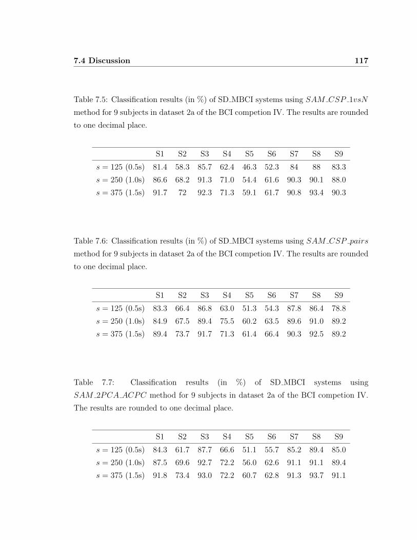
7.4 Discussion 117
Table 7.5: Classification results (in %) of SD MBCI systems using SAM CSP 1vsN
method for 9 subjects in dataset 2a of the BCI competion IV. The results are rounded
to one decimal place.
S1 S2 S3 S4 S5 S6 S7 S8 S9
s = 125 (0.5s) 81.4 58.3 85.7 62.4 46.3 52.3 84 88 83.3
s = 250 (1.0s) 86.6 68.2 91.3 71.0 54.4 61.6 90.3 90.1 88.0
s = 375 (1.5s) 91.7 72 92.3 71.3 59.1 61.7 90.8 93.4 90.3
Table 7.6: Classification results (in %) of SD MBCI systems using SAM CSP pairs
method for 9 subjects in dataset 2a of the BCI competion IV. The results are rounded
to one decimal place.
S1 S2 S3 S4 S5 S6 S7 S8 S9
s = 125 (0.5s) 83.3 66.4 86.8 63.0 51.3 54.3 87.8 86.4 78.8
s = 250 (1.0s) 84.9 67.5 89.4 75.5 60.2 63.5 89.6 91.0 89.2
s = 375 (1.5s) 89.4 73.7 91.7 71.3 61.4 66.4 90.3 92.5 89.2
Table 7.7: Classification results (in %) of SD MBCI systems using
SAM 2PCA ACPC method for 9 subjects in dataset 2a of the BCI competion IV.
The results are rounded to one decimal place.
S1 S2 S3 S4 S5 S6 S7 S8 S9
s = 125 (0.5s) 84.3 61.7 87.7 66.6 51.1 55.7 85.2 89.4 85.0
s = 250 (1.0s) 87.5 69.6 92.7 72.2 56.0 62.6 91.1 91.1 89.4
s = 375 (1.5s) 91.8 73.4 93.0 72.2 60.7 62.8 91.3 93.7 91.1

7.4 Discussion 118
Figure 7.13: Comparison of SD-MBCI and SI-MBCI classification results using
SAM CSP 1vsN for 9 subjects in dataset 2a of the BCI competition IV. The accu-
racy differences are calculated by subtracting the results of SD-MBCI from the results
of SI-MBCI. The step size 125, 250 and 375 correspond to duration of 0.5, 1 and 1.5
seconds.
Figure 7.14: Comparison of SD-MBCI and SI-MBCI classification results using
SAM CSP pairs for 9 subjects in dataset 2a of the BCI competition IV. The accu-
racy differences are calculated by subtracting the results of SD-MBCI from the results
of SI-MBCI. The step size 125, 250 and 375 correspond to duration of 0.5, 1 and 1.5
seconds.
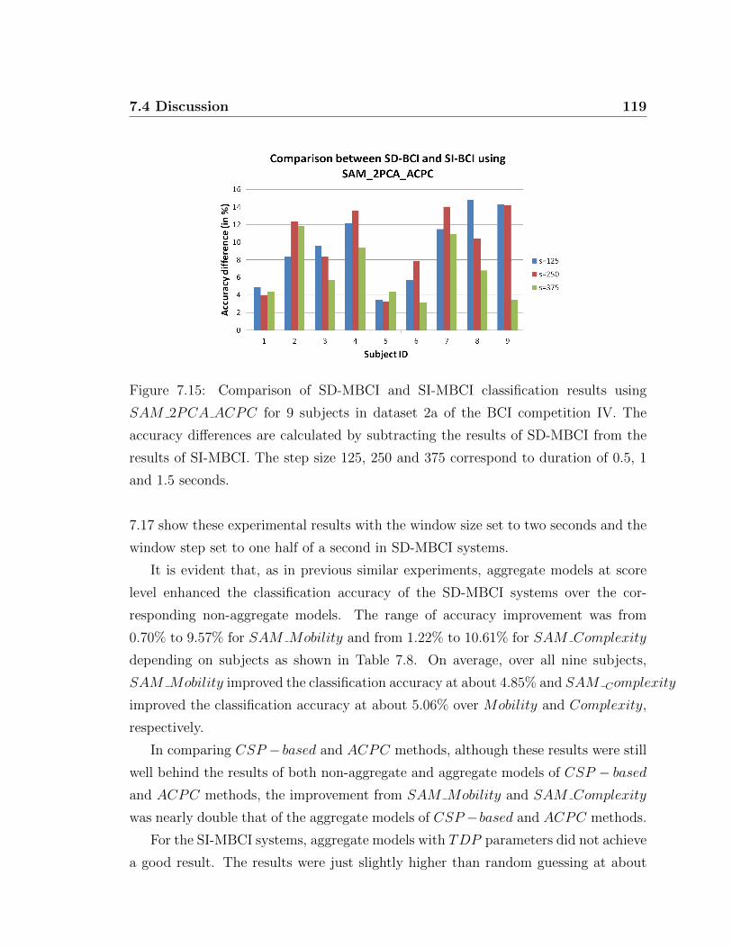
7.4 Discussion 119
Figure 7.15: Comparison of SD-MBCI and SI-MBCI classification results using
SAM 2PCA ACPC for 9 subjects in dataset 2a of the BCI competition IV. The
accuracy differences are calculated by subtracting the results of SD-MBCI from the
results of SI-MBCI. The step size 125, 250 and 375 correspond to duration of 0.5, 1
and 1.5 seconds.
7.17 show these experimental results with the window size set to two seconds and the
window step set to one half of a second in SD-MBCI systems.
It is evident that, as in previous similar experiments, aggregate models at score
level enhanced the classification accuracy of the SD-MBCI systems over the cor-
responding non-aggregate models. The range of accuracy improvement was from
0.70% to 9.57% for SAM Mobility and from 1.22% to 10.61% for SAM Complexity
depending on subjects as shown in Table 7.8. On average, over all nine subjects,
SAM Mobility improved the classification accuracy at about 4.85% and SAM Complexity
improved the classification accuracy at about 5.06% over Mobility and Complexity,
respectively.
In comparing CSP − based and ACPC methods, although these results were still
well behind the results of both non-aggregate and aggregate models of CSP − basedand ACPC methods, the improvement from SAM Mobility and SAM Complexity
was nearly double that of the aggregate models of CSP −based and ACPC methods.
For the SI-MBCI systems, aggregate models with TDP parameters did not achieve
a good result. The results were just slightly higher than random guessing at about
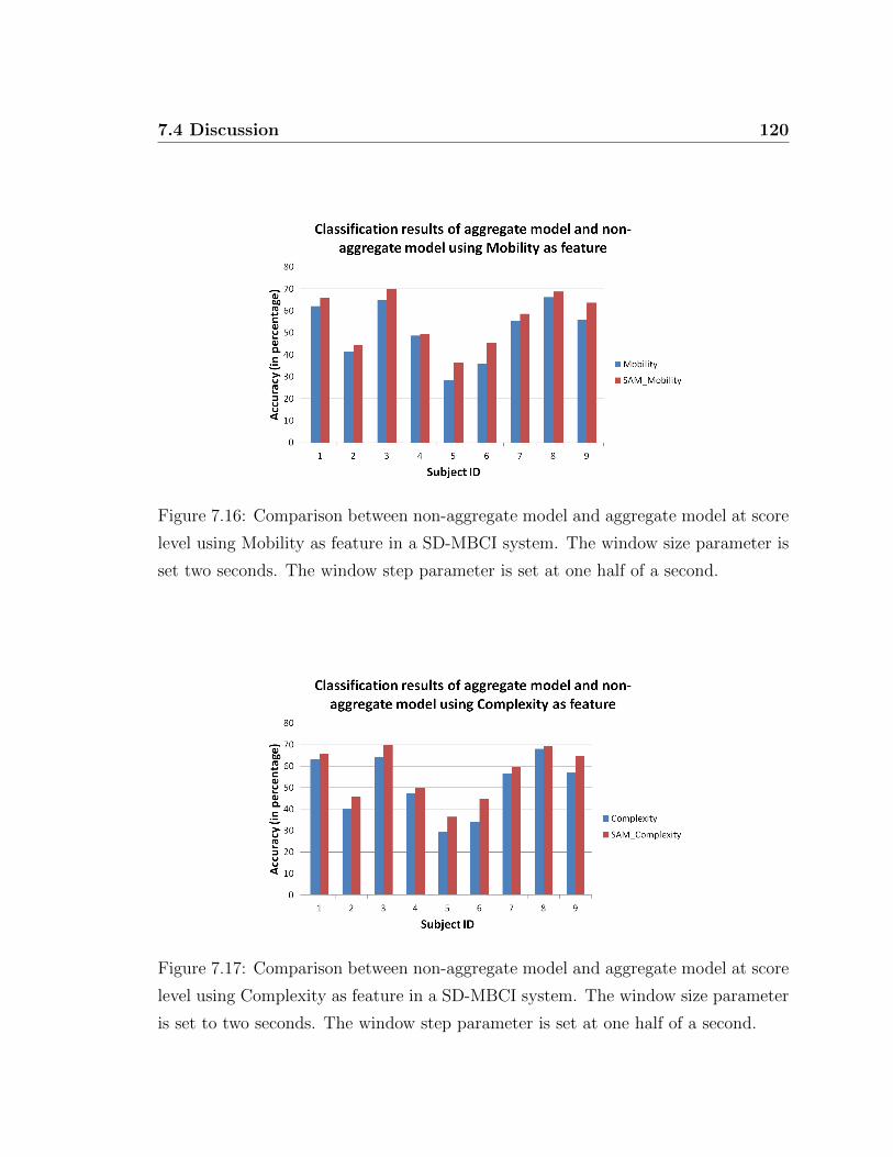
7.4 Discussion 120
Figure 7.16: Comparison between non-aggregate model and aggregate model at score
level using Mobility as feature in a SD-MBCI system. The window size parameter is
set two seconds. The window step parameter is set at one half of a second.
Figure 7.17: Comparison between non-aggregate model and aggregate model at score
level using Complexity as feature in a SD-MBCI system. The window size parameter
is set to two seconds. The window step parameter is set at one half of a second.
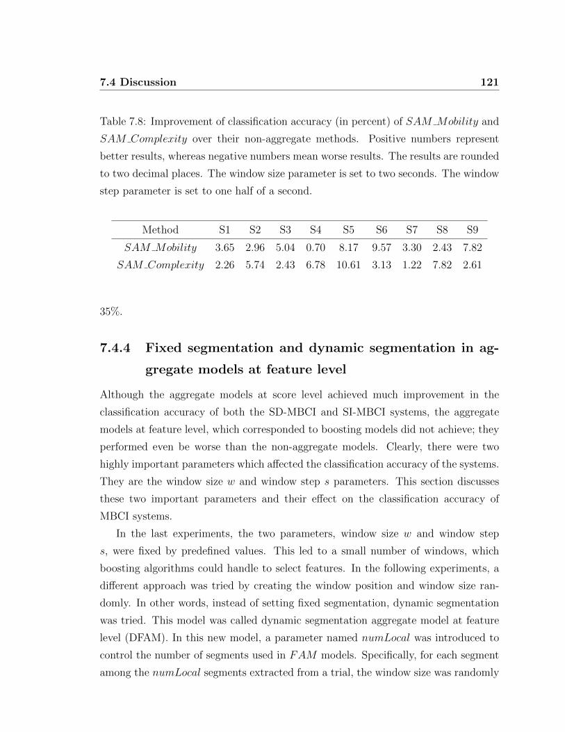
7.4 Discussion 121
Table 7.8: Improvement of classification accuracy (in percent) of SAM Mobility and
SAM Complexity over their non-aggregate methods. Positive numbers represent
better results, whereas negative numbers mean worse results. The results are rounded
to two decimal places. The window size parameter is set to two seconds. The window
step parameter is set to one half of a second.
Method S1 S2 S3 S4 S5 S6 S7 S8 S9
SAM Mobility 3.65 2.96 5.04 0.70 8.17 9.57 3.30 2.43 7.82
SAM Complexity 2.26 5.74 2.43 6.78 10.61 3.13 1.22 7.82 2.61
35%.
7.4.4 Fixed segmentation and dynamic segmentation in ag-
gregate models at feature level
Although the aggregate models at score level achieved much improvement in the
classification accuracy of both the SD-MBCI and SI-MBCI systems, the aggregate
models at feature level, which corresponded to boosting models did not achieve; they
performed even be worse than the non-aggregate models. Clearly, there were two
highly important parameters which affected the classification accuracy of the systems.
They are the window size w and window step s parameters. This section discusses
these two important parameters and their effect on the classification accuracy of
MBCI systems.
In the last experiments, the two parameters, window size w and window step
s, were fixed by predefined values. This led to a small number of windows, which
boosting algorithms could handle to select features. In the following experiments, a
different approach was tried by creating the window position and window size ran-
domly. In other words, instead of setting fixed segmentation, dynamic segmentation
was tried. This model was called dynamic segmentation aggregate model at feature
level (DFAM). In this new model, a parameter named numLocal was introduced to
control the number of segments used in FAM models. Specifically, for each segment
among the numLocal segments extracted from a trial, the window size was randomly
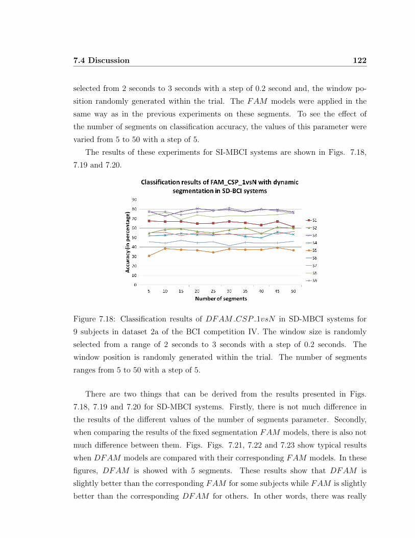
7.4 Discussion 122
selected from 2 seconds to 3 seconds with a step of 0.2 second and, the window po-
sition randomly generated within the trial. The FAM models were applied in the
same way as in the previous experiments on these segments. To see the effect of
the number of segments on classification accuracy, the values of this parameter were
varied from 5 to 50 with a step of 5.
The results of these experiments for SI-MBCI systems are shown in Figs. 7.18,
7.19 and 7.20.
Figure 7.18: Classification results of DFAM CSP 1vsN in SD-MBCI systems for
9 subjects in dataset 2a of the BCI competition IV. The window size is randomly
selected from a range of 2 seconds to 3 seconds with a step of 0.2 seconds. The
window position is randomly generated within the trial. The number of segments
ranges from 5 to 50 with a step of 5.
There are two things that can be derived from the results presented in Figs.
7.18, 7.19 and 7.20 for SD-MBCI systems. Firstly, there is not much difference in
the results of the different values of the number of segments parameter. Secondly,
when comparing the results of the fixed segmentation FAM models, there is also not
much difference between them. Figs. Figs. 7.21, 7.22 and 7.23 show typical results
when DFAM models are compared with their corresponding FAM models. In these
figures, DFAM is showed with 5 segments. These results show that DFAM is
slightly better than the corresponding FAM for some subjects while FAM is slightly
better than the corresponding DFAM for others. In other words, there was really
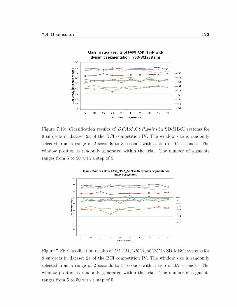
7.4 Discussion 123
Figure 7.19: Classification results of DFAM CSP pairs in SD-MBCI systems for
9 subjects in dataset 2a of the BCI competition IV. The window size is randomly
selected from a range of 2 seconds to 3 seconds with a step of 0.2 seconds. The
window position is randomly generated within the trial. The number of segments
ranges from 5 to 50 with a step of 5.
Figure 7.20: Classification results of DFAM 2PCA ACPC in SD-MBCI systems for
9 subjects in dataset 2a of the BCI competition IV. The window size is randomly
selected from a range of 2 seconds to 3 seconds with a step of 0.2 seconds. The
window position is randomly generated within the trial. The number of segments
ranges from 5 to 50 with a step of 5.

7.4 Discussion 124
no difference between DFAM and FAM . This observation was confirmed by taking
an average over nine subject results as shown in Table 7.9. The differences were less
than 1% and quite small. It was noted that DFAM models have more computation
cost than corresponding FAM models.
Figure 7.21: Comparison between FAM CSP 1vsN and its corresponding
DFAM CSP 1vsN with 5 dynamic segments in SD-MBCI systems for 9 subjects
in dataset 2a of the BCI competition IV. The window size is randomly selected from
a range of 2 seconds to 3 seconds with a step of 0.2 seconds. The window position
is randomly generated within the trial. The number of segments ranges from 5 to 50
with a step of 5.
Similar evaluations can be made regarding the subject-independent MBCI exper-
iments. In conclusion, there is not much difference between fixed segmentation and
dynamic segmentation aggregate models at feature level in the experiments conducted
with both SD and SI MBCI systems.
7.4.5 Toward online multi-class BCI systems
It is easy to see that the proposed general aggregate models at score level in Fig.
6.3 can be extended to handle online multi-class BCI systems with little modification
and little additional processing time. Excluding the parameters of feature extraction
methods and classifiers, the method proposed here introduces only two additional
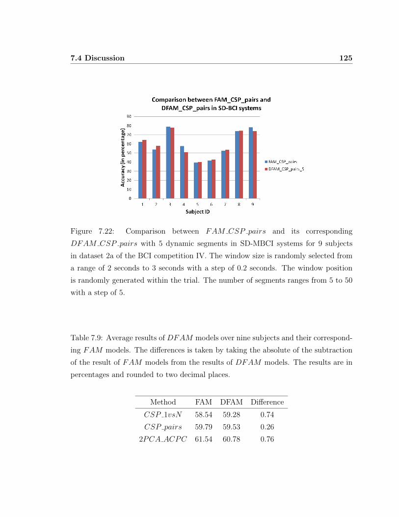
7.4 Discussion 125
Figure 7.22: Comparison between FAM CSP pairs and its corresponding
DFAM CSP pairs with 5 dynamic segments in SD-MBCI systems for 9 subjects
in dataset 2a of the BCI competition IV. The window size is randomly selected from
a range of 2 seconds to 3 seconds with a step of 0.2 seconds. The window position
is randomly generated within the trial. The number of segments ranges from 5 to 50
with a step of 5.
Table 7.9: Average results of DFAM models over nine subjects and their correspond-
ing FAM models. The differences is taken by taking the absolute of the subtraction
of the result of FAM models from the results of DFAM models. The results are in
percentages and rounded to two decimal places.
Method FAM DFAM Difference
CSP 1vsN 58.54 59.28 0.74
CSP pairs 59.79 59.53 0.26
2PCA ACPC 61.54 60.78 0.76
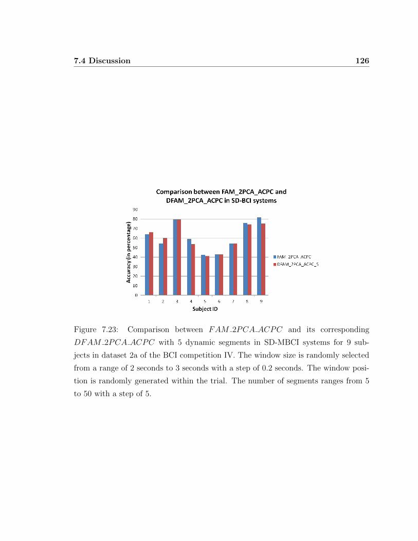
7.4 Discussion 126
Figure 7.23: Comparison between FAM 2PCA ACPC and its corresponding
DFAM 2PCA ACPC with 5 dynamic segments in SD-MBCI systems for 9 sub-
jects in dataset 2a of the BCI competition IV. The window size is randomly selected
from a range of 2 seconds to 3 seconds with a step of 0.2 seconds. The window posi-
tion is randomly generated within the trial. The number of segments ranges from 5
to 50 with a step of 5.
7.4 Discussion 127
parameters, namely window size w and window step s. This proposed method is
independent with feature extractors such as CSP − based or ACPC analysis and
classifiers such as SVM . CSP − based analysis and SVM were adopted in these
experiments because they are state-of-the-art methods in motor imagery-based BCI
systems. Moreover, the window size parameter is similar to the trial length parameter.
This means that whether using the proposed method or not, it was still necessary
to determine this parameter. In short, the proposed method adds only one more
parameter namely the window step s.
On the matter of complexity of computation in online multi-class BCI systems,
the proposed method is very efficient. As shown in Fig. 6.3, assuming that K
frames were needed for making a decision, from the (K + 1)− th frame onwards, the
results obtained from the previous K − 1 frames could be reused. It only needs to
extract feature and perform classification on the K-th frame. The computation cost
for the aggregate function is not significant as shown in Eq. 6.2 in Chapter 6, and
hence the computation cost from the (K + 1)− th frame onwards is nearly the same
as that in a non-aggregate model which only depends on the computation cost for
feature extraction and classification methods. For some first frames, due to the lack
of sufficient number of frames for the aggregate function, some boundary handling
techniques can be applied.
In summary, with only one additional parameter and a very small difference in the
computation costs between the proposed aggregate model and other non-aggregate
models, the general aggregate model at score level can easily be implemented in online
multi-class BCI systems.

Chapter 8
Conclusions and Future Research
8.1 Conclusions
This thesis has presented the research on new feature extraction methods for motor
imagery-based multi-class BCI systems. The research was limited on BCI systems
which use EEG as an brain signal acquisition method. The research has sought to
know whether interaction between channels can result in features that can achieve
better classification accuracy than of features which are extracted from individual
channels in motor imagery-based MBCI systems. A review of state-of-the-art feature
extraction methods in motor imagery-based BCI systems led to the decision to use
the methodology of using information of interaction between channels for building
spatial filters in order to enhance spatial quality of brain signals. Such spatial filters
in 2-class BCI systems are well defined but have still not been solved in multi-class
BCI systems. Solving problems on multi-class BCI systems relies on several vital
questions. The study tried to answer three of these questions:
1. How can we build a feature extraction method based on synchronization mea-
sures that targets multi-class BCI systems directly instead of through a set of
2-class problems?
2. How can we build a feature extraction method that overcomes the issue of large
inter-subject and inter-session variability in multi-class BCI systems?
3. What is the difference in performance between subject-dependent and subject-
129

8.1 Conclusions 130
independent MBCI systems? What feature extraction methods can be used in
subject-independent MBCI systems for enhancing performance? What models
can be used in both subject-dependent and subject-independent MBCI systems?
On the way to finding answers for these questions, the research proposed two
new feature extraction methods. The first proposed method is called Approxima-
tion Common Principal Components analysis (ACPC). In order to materialize this
method, two specific methods were proposed called Jacobian-based Approximation
Common Principal Components (Jacobi ACPC) and 2-PCA Approximation Com-
mon Principal Components (2PCA ACPC). While the Jacobi ACPC method is
an extension of a well known diagonalization based on the Jacobian rotation, the
2PCA ACPC attempts to form new perpendicular components by approximating
all original components of input brain signals. The second proposed method is based
on aggregate models. Specifically, two general aggregate models were proposed: one
at score level and one at feature level. Theoretical background of the two proposed
methods were presented in Chapters 4 and 6, respectively. Experiments of these two
feature extraction methods were conducted on a well known and widely used dataset
for multi-class BCI systems, namely the Dataset 2a of the BCI Competition IV. This
dataset is well suited to not only multi-class BCI systems but also multi-subject BCI
experiments, and for both subject-dependent and subject-independent systems. The
experimental findings are chapter specific, shown in Chapters 5 and 7. In this section,
the experimental findings are synthesized to answer the study’s research questions.
1. How can we build a feature extraction method based on synchronization mea-
sures that targets multi-class BCI systems directly instead of through a set of
2-class problems?
2PCA ACPC directly targets multi-class BCI systems by approximating components
of original brain signals. 2PCA ACPC explores the correlation between the channels
of input brain signal to enhance the spatial quality of the signal, and then extracts fea-
tures. This is done directly with provided data which has more than two classes. It is
different from other methods that are based on 2-class problem solvers. Such methods
try to solve a multi-class problem by converting it into several 2-class sub-problems,
solving them separately and then combining the sub-problem solutions to form a solu-
tion to the original multi-class problem. Two typical strategies of this conversion are
8.1 Conclusions 131
One-versus-the-rest (1vsN) and pair-wise (pairs). They both can actually be called
Union-based Common Principal Components analysis due to the fact that they form
components of sub-problems separately and then take the union of all of them to-
gether. In experiments, Common Spatial Patterns (CSP ), which is a state-of-the-art
method for motor imagery-based 2-class BCI system, was chosen as the 2-class prob-
lem solver. The study compared 2PCA ACPC with CSP 1vsN and CSP pairs.
It also compared 2PCA ACPC with another feature extractor based on individual
channels called Time Domain Parameters. The study found that the 2PCA ACPC
method achieved better classification results then the two CSP -based methods in
eight out of nine subjects. The classification accuracy improvement ranged from 1%
to 10% depending on the subject. On average over all nine subjects participating
in the experiment, 2PCA ACPC improved about 3.5% compared with CSP 1vsN
and about 4.1% compared with CSP pairs. It is evident that both ACPC meth-
ods significantly outperformed two time domain features Mobility and Complexity
on all subjects. When compared with TDP features, the classification accuracy im-
provement ranged from 11% to 23% for 2PCA ACPC. Overall, 2PCA ACPC im-
proved about 16.6% compared with TDP features on average, over all nine subjects
participating in the experiment. These findings show that 2PCA ACPC, which is
based on multi-channel information not only is better than a typical individual chan-
nel features such as TDP but also outperforms other 2-class solver-based strategies
employing CSP , a state-of-the-art method for motor imagery-based 2-class BCI sys-
tems. Another advantage of 2PCA ACPC is that it can be visualized based on its
components’ coefficients. This property helps researchers explain how 2PCA ACPC
operates when extracting features from brain signals.
2. How can we build a feature extraction method that overcomes the issue of large
inter-subject and inter-session variability in multi-class BCI systems?
Two general aggregate models were proposed for the purpose of dealing with the
high inter-subject and inter-session variability in multi-class BCI systems. The first
is called aggregate model at score level (SAM). The second is called aggregate model
at feature level (FAM). The main idea of these general aggregate models is that
they treat a trial as a set of possibly overlapped segments instead of as a whole
trial. By this means, these aggregate models can eliminate the effects of the delay
8.1 Conclusions 132
and activation issue which is a well known main factor in making high inter-subject
and inter-session variability in multi-class BCI systems. These two general models
can be used with all existing features. The research experimented with these two
models using CSP -based, 2PCA ACPC and TDP methods for extracting features.
Experimental results show that the aggregate models with these features at score level
are better than, or at least equal to, their corresponding non-aggregate models for
most subjects in the dataset 2a of the BCI competition IV used in the experiments.
On average, over all nine subjects, the aggregate models at score level of CSP 1vsN ,
CSP pairs and 2PCA ACPC improved about 2.4%, 2.9% and 2.0% respectively over
their original methods. For single-channel features such as TDP , on average over all
nine subjects, SAM Mobility improved the classification accuracy about 4.9% and
SAM Complexity improved the classification accuracy about 5.1% over Mobility
and Complexity, respectively.
3. What is the difference in performance between subject-dependent and subject-
independent MBCI systems? What feature extraction methods can be used in
subject-independent MBCI systems for enhancing performance? What models
can be used in both subject-dependent and subject-independent MBCI systems?
From current knowledge of the basic principles of aggregate models and the nature
of brain signals, the research proved that aggregate models can be used not only
in SD-MBCI but also in SI-MBCI systems. The experimental results in SI-MBCI
were fairly consistent with those in SD-MBCI. While the aggregate models at score
level showed higher classification accuracy than their corresponding non-aggregate
models, the aggregate models at feature level showed much lower classification accu-
racy. The best improvement of classification was with SAM 2PCA ACPC compared
with its corresponding non-aggregate model SAM 2PCA ACPC which was about
4.77%. SAM CSP 1vsN and SAM CSP pairs enhanced about 1.15% and 2.93%
over CSP 1vsN and CSP pairs, respectively. To the best of the author’s knowledge,
this is the first study conducting experiments with SI-MBCI systems. The experi-
ments using the proposed methods on SI-2MBCI showed that aggregate models were
better than the non-aggregate models and the non-aggregate models were better than
those reported by Lotte et. al. [Lotte et al., 2009]. Two one-way ANOVA tests on
8.1 Conclusions 133
factor of step size s showed that there was a significant difference between the val-
ues of the step size s. Therefore, with an appropriate selection of the window step
parameter, the aggregate models at score level achieved notably higher classification
accuracy results than the corresponding non-aggregate models.
Although aggregate models can reduce the effects of high inter-subject and inter-
session variability in SI-MBCI systems, the problem of SI-MBCI systems were still
more complicated than the one of SD-MBCI systems. The classification results using
aggregate models in SD-MBCI systems were greater than with SI-MBCI systems.
This conclusion was confirmed with experimental results in 2-class BCI systems. The
range of accuracy differences between SD-BCI and SI-BCI systems was very high
from 0.0% to 28.2% depending on step size s, subjects and aggregate models.
Finding answers for these research questions led to the development of a new
feature extraction method, one in which a spatial filters method is used in a aggre-
gate model. This new method can be called segmented spatial filters. The spatial
filters method, which is based on the multi-variate model, has been proven to have
advantages over univariate models in motor imagery-based BCI systems. Inheriting
advantages from the spatial filters and aggregate models, the segmented spatial filters
method can further enhance the performance of motor imagery-based BCI systems.
It has the following advantages:
• It improves the spatial resolution of EEG signals;
• It efficiently deals with inter-subject and inter-session variability in brain signals;
• It can be visualized so that it can be interpreted by researchers;
• It can be used in both subject-dependent and subject-independent BCI systems;
• It is very efficient and straight forward to apply in online BCI systems from a
corresponding off-line version.
Specifically, for the proposed method ACPC which directly targets multi-class BCI
systems, the experimental investigation showed that the segmented ACPC method
has all the above-listed advantages for multi-class BCI systems.
8.2 Future research 134
8.2 Future research
Given the results and drawing on the the discussions reported in this study, three
directions are clearly evident for future research. They are
• Extending aggregate models in order to handle the problem of brain signal
segmentation. As shown in the study and indicated in other related research,
subjects can lose their attention during BCI experiments. This means that not
all data in the trial is meaningful and helpful. Brain signal segmentation can
extract meaningful and helpful portions of the trial. This direction has gained
attention from brain signal researchers in epilepsy detection. From this research
it has been clear that BCI researchers also need to focus on the brain signal
segmentation problem.
• Designing motor imagery-based BCI systems with longer experimental time pe-
riods. The effect of high inter-subject and inter-session variability has forced
motor imagery-based BCI system designers to use short durations in their ex-
periments. Using aggregate models and segmented spatial filters, this effect can
be reduced. Therefore, experiment designers now can extend the duration of
the experiments. It is the first step towards truly streaming BCI systems.
• Testing and developing aggregate models with other features relevant to other
BCI problems. This study focuses on the motor imagery-based BCI problem
only. In a motor imagery-based BCI system, subjects are asked to concentrate
on interacting with devices. This property makes aggregate models suitable for
motor imagery-based BCI systems. However, in different BCI systems where
other control signals are used, this property might not be kept. Therefore,
aggregate models need to be modified to adapt to the new properties of these
BCI systems.

Appendices
Corolarry 1. Given a real symmetrical matrix A and a basic Jacobi rotation matrix
R. Let B be the resulted matrix after applying the Jacobi rotation. There is no
difference between the Frobenius norms of the two matrices. It means that
||B||F = ||A||F . (8.1)
Proof. As definition of the Jacobi rotation, we have:
B = RTAR (8.2)
The Frobenius norm is defined as
||A||F =∑i,j
A2i,j = trace(AAT ) (8.3)
where A is a symmetrical matrix. Therefore,
||B||F = ||RTAR||F (8.4)
= trace((RTAR)(RTAR)T ) (8.5)
= trace(A)trace((A)T ) (8.6)
= ||A||F (8.7)
Corolarry 2. Given a real symmetrical matrix A and a basic Jacobi rotation matrix
R at the row p and the column q. Let B be the resulted matrix after applying the Jacobi
rotation. Let S(.) be the function of the sum of square of all off-diagonal elements of
a matrix. Then we have,
S(B) = S(A)− 2× |Ap,q|2 (8.8)
135

136
Proof. Let A′ and B′ be the matrix just contain only four elements of the matrix
A and B respectively. Let c = cosθ and s = sinθ. Without any loss, the matrix
manipulation can be reduced by applying the rotation matrix R on the matrix A as
follows.(Bp,p Bp,q
Bq,p Bq,q
)=
(cosθ sinθ
−sinθ cosθ
)(Ap,p Ap,q
Aq,p Aq,q
)(cosθ −sinθsinθ cosθ
)(8.9)
=
(cAp,p + sAq,p cAp,q + sAq,q
−sAp,p + cAq,p −sAp,q + cAq,q
)(c −ss c
)(8.10)
=
(c2Ap,p + s2Aq,q + scAp,q + scAq,p −csAp,p + csAq,q + c2Ap,q − s2Aq,p−scAp,p + csAq,q − s2Ap,q + c2Aq,p s2Ap,p + c2Aq,q − csAp,q − csAq,p
)(8.11)
=
(c2Ap,p + s2Aq,q + 2scAp,q cs(Aq,q − Ap,p) + Ap,q(c
2 − s2)cs(Aq,q − Ap,p) + Ap,q(c
2 − s2) s2Ap,p + c2Aq,q − 2csAp,q
)(8.12)
Eliminating off-diagonal elements means that Bp,q = Bq,p = 0. Therefore,
cosθsinθ(Aq,q − Ap,p) + (cos2θ − sin2θ)Ap,q = 0 (8.13)
⇔ cos2θAp,q +1
2sin2θ(Aq,q − Ap,p) = 0 (8.14)
⇔ tan2θ =−2Ap,q
Aq,q − Ap,p(8.15)
The appropriate value of the angle θ in the Jacobi rotation matrix is given by the Eq.
8.15. Moreover, because there is no difference between the Frobenius norms of the
two matrices A and B, proven in Corollary 1, we have S(A) − S(B) = A2i,j + A2
j,i =
2A2i,j.
Lemma 1. Given a real symmetrical matrix Cti and a basic Jacobi rotation matrix
R(p, q, θ), with appropriate value of θ, the sum of non-diagonal elements St can be
reduced by 2× |Cti (p, q)|2. It means that
St+1i = Sti − 2× |Ct
i (p, q)|2 (8.16)
Proof. The lemma is directly proven by replacing the matrix Cti by A, the matrix
Ct+1i by B, the Jacobi rotation matrix R(p, q, θ) by R, and the function Sti , S
t+1i by
the function S(A), S(B) respectively, according to Corollary 2.

My Research Publications
1. Tuan Hoang, Phuoc Nguyen, Trung Le, Dat Tran, Dharmendra Sharma. Enhancing
Performance of SVM-Based Brain-Computer Interface Systems. Special
ICONIP issue of the Australian Journal of Intelligent Information Systems, 2010.
2. Tuan Hoang, Dat Tran, Xu Huang. Approximation-based Common Principal
Component for feature extraction in Multi-class Brain-Computer Inter-
faces. The 35th Annual International Conference of the IEEE EMBS (EMBC 2013),
July, 2013.
3. Tuan Hoang, Dat Tran, Xu Huang and Wanli Ma. A General Aggregate Model
for Improving Multi-Class Brain-Computer Interface Systems Performance.
The International Joint Conference on Neural Networks (IJCNN) 2013.
4. Tuan Hoang, Dat Tran, Khoa Truong, Trung Le, Xu Huang, Dharmendra Sharma
and Toi Vo. Time Domain Parameters for Online Feedback fNIRS-based
Brain-Computer Interface Systems. The 19th International Conference on Neu-
ral Information Processing (ICONIP 2012), Part II, LNCS 7664, pp. 192201, 2012.
5. Tuan Hoang, Dat Tran, Khoa Truong, Phuoc Nguyen, Xu Huang, Dhamendra Sharma,
Toi Vo. Experiments on Synchronous Nonlinear Features for 2-Class NIRS-
based Motor Imagery Problem. The 4th International Conference on The De-
velopment of Biomedical Engineering, 2012.
6. Tuan Hoang, Dat Tran, Xu Huang, Dhamendra Sharma, Khoa Truong, Toi Vo. High
order moment features for NIRs-based classification problems. The 4th
International Conference on The Development of Biomedical Engineering, 2012.
7. Phuoc Nguyen, Dat Tran, Trung Le, Tuan Hoang and Dharmendra Sharma. Multi-
Sphere Support Vector Data Description for Brain-Computer Interface.
137

138
The International Conference on Communications and Electronics (ICCE), pp. 318-
321, 2012.
8. Trung Le, Dat Tran, Tuan Hoang and Dharmendra Sharma. Maximal Margin
Kernel Learning Vector Quantisation for Binary Classification. The 19th
International Conference on Neural Information Processing (ICONIP 2012), Part III,
LNCS 7665, pp. 191198, 2012.
9. Trung Le, Dat Tran, Tuan Hoang, Wanli Ma and Dharmendra Sharma. Generalised
Support Vector Machine for Brain-Computer Interface. The 18th Interna-
tional Conference on Neural Information Processing (ICONIP 2011), Lecture Notes
in Computer Science, vol. 7062, pp. 692-700, 2011.
10. Tuan Hoang, Dat Tran, Phuoc Nguyen, Xu Huang, Dharmendra Sharma. Exper-
iments on Using Combined Short Window Bivariate Autoregression for
EEG Classification. The 5th International IEEE EMBS Conference on Neural
Engineering, NER 2011, Mexico, 2011.

Bibliography
[BCI, 2008] (2008). Results on dataset 2a of the bci competition iv.
[Anderson et al., 1998] Anderson, C. W., Stolz, E. A., and Shamsunder, S. (1998).
Multivariate autoregressive models for classification of spontaneous electroen-
cephalogram during mental tasks. IEEE Transactions on Biomedical Engineering,
45:277–286.
[Andrzejak et al., 2001] Andrzejak, R. G., Lehnertz, K., Mormann, F., Rieke, C.,
David, P., and Elger, C. E. (2001). Indications of nonlinear deterministic and
finite-dimensional structures in time series of brain electrical activity: Dependence
on recording region and brain state. Phys. Rev. E, 64:061907.
[Ang et al., 2008] Ang, K. K., Chin, Z. Y., Zhang, H., and Guan, C. (2008). Filter
bank common spatial pattern (fbcsp) in brain-computer interface. In IJCNN, pages
2390–2397. IEEE.
[Ang et al., 2012] Ang, K. K. K., Chin, Z. Y. Y., Wang, C., Guan, C., and Zhang,
H. (2012). Filter bank common spatial pattern algorithm on BCI competition IV
datasets 2a and 2b. Frontiers in neuroscience, 6.
[Ariely and Berns, 2010] Ariely, D. and Berns, G. S. (2010). Neuromarketing: the
hope and hype of neuroimaging in business. Nature Reviews Neuroscience,
11(4):284–292.
[Arthurs and Boniface, 2003] Arthurs, O. and Boniface, S. (2003). What aspect of
the fmri {BOLD} signal best reflects the underlying electrophysiology in human
somatosensory cortex? Clinical Neurophysiology, 114(7):1203 – 1209.
139
BIBLIOGRAPHY 140
[Arvaneh et al., 2011] Arvaneh, M., Guan, C., Ang, K. K., and Quek, C. (2011).
Optimizing the channel selection and classification accuracy in eeg-based bci. IEEE
Trans. Biomed. Engineering, 58(6):1865–1873.
[Asensio-Cubero et al., 2011] Asensio-Cubero, J., Galvan, E., Panlaniappan, R., and
Gan, J. Q. (2011). Wavelet design by means of multi-objective gas for motor im-
agery eeg analysis. In The 5th International Brain-Computer Interface Conference,
pages 60–63. Verlag der Technischen Universitat Graz.
[Balli and Palaniappan, 2010] Balli, T. and Palaniappan, R. (2010). Classification of
biological signals using linear and nonlinear features. Physiological Measurement,
31(7):903+.
[Bashashati et al., 2007] Bashashati, A., Fatourechi, M., Ward, R. K., and Birch,
G. E. (2007). A survey of signal processing algorithms in braincomputer interfaces
based on electrical brain signals. Journal of Neural Engineering, 4(2):R32.
[Bell and Sejnowski, 1995] Bell, A. J. and Sejnowski, T. J. (1995). An information-
maximization approach to blind separation and blind deconvolution. Neural Com-
putation, 7:1129–1159.
[Belouchrani et al., 1997] Belouchrani, A., Abed-meraim, K., Cardoso, J.-F.,
Moulines, E., Member, I., Member, I., Member, I., and Member, I. (1997). A
blind source separation technique using second order statistics.
[Blankertz et al., 2008a] Blankertz, B., Tomioka, M. K. R., Hohlefeld, F. U., Nikulin,
V., and robert Mller, K. (2008a). Invariant common spatial patterns: Alleviating
nonstationarities in brain-computer interfacing. In In Ad. in NIPS 20, page 2008.
MIT Press.
[Blankertz et al., 2008b] Blankertz, B., Tomioka, R., Lemm, S., Kawanabe, M., and
robert Mller, K. (2008b). Optimizing spatial filters for robust eeg single-trial anal-
ysis. In IEEE Signal Proc. Magazine, pages 581–607.
[Boostani and Moradi, 2004] Boostani, R. and Moradi, M. H. (2004). A new ap-
proach in the bci research based on fractal dimension as feature and adaboost as
classifier. Journal of Neural Engineering, 1(4):212.

BIBLIOGRAPHY 141
[Brodu et al., 2011] Brodu, N., Lotte, F., and Lecuyer, A. (2011). Comparative Study
of Band-Power Extraction Techniques for Motor Imagery Classification. In IEEE
Symposium on Computational Intelligence, Cognitive Algorithms, Mind, and Brain
(SSCI’2011 CCMB), pages 1–6, Paris, France. IEEE.
[Brunner et al., 2007] Brunner, C., 0003, M. N., Leeb, R., Graimann, B., and
Pfurtscheller, G. (2007). Spatial filtering and selection of optimized components in
four class motor imagery eeg data using independent components analysis. Pattern
Recognition Letters, 28(8):957–964.
[Brunner et al., 2010] Brunner, C., Billinger, M., and Neuper, C. (2010). A compar-
ison of univariate, multivariate, bilinear autoregressive, and bandpower features
for brain-computer interfaces. In The 4th International Brain-Computer Interface
Conference. Verlag der Technischen Universitat Graz.
[Brunner et al., 2011] Brunner, C., Billinger, M., Vidaurre, C., and Neuper, C.
(2011). A comparison of univariate, vector, bilinear autoregressive and band power
features for brain-computer interfaces. Medical and Biological Engineering and
Computing, 49:1337–1346.
[Brunner et al., 2008] Brunner, C., Leeb, R., Muller-Putz, G., Schlogl, A., and
Pfurtscheller, G. (2008). Bci competition 2008–graz data set a. Institute for
Knowledge Discovery (Laboratory of Brain-Computer Interfaces), Graz University
of Technology.
[Chin et al., 2009] Chin, Z. Y., Ang, K. K., Wang, C., Guan, C., and Zhang, H.
(2009). Multi-class filter bank common spatial pattern for four-class motor imagery
bci. In Engineering in Medicine and Biology Society, 2009. EMBC 2009. Annual
International Conference of the IEEE, pages 571–574. IEEE.
[Cichocki et al., 2008] Cichocki, A., Washizawa, Y., Rutkowski, T., Bakardjian, H.,
Phan, A.-H., Choi, S., Lee, H., Zhao, Q., Zhang, L., and Li, Y. (2008). Noninvasive
bcis: Multiway signal-processing array decompositions. Computer, 41(10):34–42.
[Cona et al., 2009] Cona, F., Zavaglia, M., Astolfi, L., Babiloni, F., and Ursino, M.
(2009). Changes in eeg power spectral density and cortical connectivity in healthy
BIBLIOGRAPHY 142
and tetraplegic patients during a motor imagery task. Comp. Int. and Neurosc.,
2009.
[Coppersmith et al., 1999] Coppersmith, D., Hong, S. J., and Hosking, J. R. M.
(1999). Partitioning nominal attributes in decision trees. Data Min. Knowl. Dis-
cov., 3(2):197–217.
[Decety, 1996] Decety, J. (1996). The neurophysiological basis of motor imagery.
Behavioural Brain Research, 77(12):45 – 52.
[Dornhege et al., 2004] Dornhege, G., Blankertz, B., Curio, G., and Muller, K. R.
(2004). Boosting bit rates in noninvasive EEG single-trial classifications by feature
combination and multiclass paradigms. IEEE Trans. Biomed. Eng., 51(6):993–
1002.
[Dressler et al., 2004] Dressler, O., Schneider, G., Stockmanns, G., and Kochs, E.
(2004). Awareness and the EEG power spectrum: analysis of frequencies. British
Journal of Anaesthesia, 93(6):806.
[Drucker et al., 1993] Drucker, H., Schapire, R. E., and Simard, P. (1993). Boosting
performance in neural networks. IJPRAI, 7(4):705–719.
[Ellis, 1997] Ellis, D. (1997). Chapter 22. In Hardcastle, W. J. and Laver, J., ed-
itors, The Handbook of phonetic sciences, number 4 in Blackwell Handbooks in
Linguistics, chapter 22, pages 757–780. Blackwell Publishers Ltd, Oxford.
[Emotiv, 2013] Emotiv (2013). accessed on 28 august 2013. http://emotiv.com.
[Falzon et al., 2012] Falzon, O., Camilleri, K. P., and Muscat, J. (2012). The ana-
lytic common spatial patterns method for eeg-based bci data. Journal of Neural
Engineering, 9(4):045009.
[Fatourechi et al., 2007] Fatourechi, M., Bashashati, A., Ward, R. K., and Birch,
G. E. (2007). EMG and EOG artifacts in brain computer interface systems: A
survey. Clinical neurophysiology, 118(3):480–494.
[Fazli et al., 2012] Fazli, S., Mehnert, J., Steinbrink, J., Curio, G., Villringer, A.,
Mller, K.-R., and Blankertz, B. (2012). Enhanced performance by a hybrid nirseeg

BIBLIOGRAPHY 143
brain computer interface. NeuroImage, 59(1):519 – 529. ¡ce:title¿Neuroergonomics:
The human brain in action and at work¡/ce:title¿.
[Fazli et al., 2009] Fazli, S., Popescu, F., Danczy, M., Blankertz, B., Mller, K.-R.,
and Grozea, C. (2009). Subject-independent mental state classification in single
trials. Neural Networks, 22(9):1305–1312.
[Fiebach et al., 2005] Fiebach, C. J., Gruber, T., and Supp, G. G. (2005). Neuronal
mechanisms of repetition priming in occipitotemporal cortex: Spatiotemporal ev-
idence from functional magnetic resonance imaging and electroencephalography.
Journal of Neuroscience, 25(13):3414–3422.
[Flury, 1988] Flury, B. (1988). Common principal components and related multivari-
ate models. Wiley, New York.
[Freund and Schapire, 1995] Freund, Y. and Schapire, R. E. (1995). A decision-
theoretic generalization of on-line learning and an application to boosting. In
Proceedings of the Second European Conference on Computational Learning The-
ory, EuroCOLT ’95, pages 23–37, London, UK, UK. Springer-Verlag.
[Freund and Schapire, 1996] Freund, Y. and Schapire, R. E. (1996). Experiments
with a New Boosting Algorithm. In International Conference on Machine Learning,
pages 148–156.
[Freund and Schapire, 1997] Freund, Y. and Schapire, R. E. (1997). A decision-
theoretic generalization of on-line learning and an application to boosting. J.
Comput. Syst. Sci., 55(1):119–139.
[Fujioka, 1993] Fujioka, T. (1993). An approximate test for common principal com-
ponent subspaces in two groups. Annals of the Institute of Statistical Mathematics,
45(1):147–158.
[Gautama et al., 2003] Gautama, T., Mandic, D. P., and Van Hulle, M. M. (2003).
Indications of nonlinear structures in brain electrical activity. Phys. Rev. E,
67:046204.
BIBLIOGRAPHY 144
[Gottemukkula and Derakhshani, 2011] Gottemukkula, V. and Derakhshani, R.
(2011). Classification-guided feature selection for nirs-based bci. In Neural Engi-
neering (NER), 2011 5th International IEEE/EMBS Conference on, pages 72–75.
[Gouy-Pailler et al., 2010] Gouy-Pailler, C., Congedo, M., Brunner, C., Jutten, C.,
and Pfurtscheller, G. (2010). Nonstationary brain source separation for multiclass
motor imagery. IEEE Trans. Biomed. Engineering, 57(2):469–478.
[Gouy-Pailler et al., 2008] Gouy-Pailler, C., Congedo, M., Brunner, C., Jutten, C.,
Pfurtscheller, G., et al. (2008). Multi-class independent common spatial patterns:
Exploiting energy variations of brain sources.
[Graimann et al., 2010] Graimann, B., Allison, B., and Pfurtscheller, G. (2010).
BrainComputer Interfaces: A Gentle Introduction.
[Grosse-Wentrup and Buss, 2008] Grosse-Wentrup, M. and Buss, M. (2008). Multi-
class common spatial patterns and information theoretic feature extraction. IEEE
Trans. Biomed. Engineering, 55(8):1991–2000.
[Gurkok and Nijholt, 2012] Gurkok, H. and Nijholt, A. (2012). Brain-computer in-
terfaces for multimodal interaction: A survey and principles. Int. J. Hum. Comput.
Interaction, 28(5):292–307.
[Gysels and Celka, 2004] Gysels, E. and Celka, P. (2004). Phase synchronization for
the recognition of mental tasks in a brain-computer interface. Neural Systems
and Rehabilitation Engineering, IEEE Transactions on [see also IEEE Trans. on
Rehabilitation Engineering], 12(4):406–415.
[Hanakawa et al., 2008] Hanakawa, T., Dimyan, M. A., and Hallett, M. (2008). Motor
planning, imagery, and execution in the distributed motor network: A time-course
study with functional mri. Cerebral Cortex, 18(12):2775–2788.
[Hanakawa et al., 2003] Hanakawa, T., Immisch, I., Toma, K., Dimyan, M. A.,
Van Gelderen, P., and Hallett, M. (2003). Functional properties of brain ar-
eas associated with motor execution and imagery. Journal of Neurophysiology,
89(2):989–1002.
BIBLIOGRAPHY 145
[Herff et al., 2012] Herff, C., Heger, D., Putze, F., Guan, C., and Schultz, T. (2012).
Cross-subject classification of speaking modes using fnirs. In Huang, T., Zeng,
Z., Li, C., and Leung, C., editors, Neural Information Processing, volume 7664 of
Lecture Notes in Computer Science, pages 417–424. Springer Berlin Heidelberg.
[Hoang et al., 2013a] Hoang, T., Tran, D., Truong, K., Nguyen, P., Vo Van, T.,
Huang, X., and Sharma, D. (2013a). Experiments on synchronous nonlinear fea-
tures for 2-class nirs-based motor imagery problem. In Toi, V. V., Toan, N. B.,
Dang Khoa, T. Q., and Lien Phuong, T. H., editors, 4th International Conference
on Biomedical Engineering in Vietnam, volume 40 of IFMBE Proceedings, pages
8–12. Springer Berlin Heidelberg.
[Hoang et al., 2013b] Hoang, T., Tran, D., Truong, K., Nguyen, P., Vo Van, T.,
Huang, X., and Sharma, D. (2013b). High order moment features for nirs-based
classification problems. In Toi, V. V., Toan, N. B., Dang Khoa, T. Q., and
Lien Phuong, T. H., editors, 4th International Conference on Biomedical Engi-
neering in Vietnam, volume 40 of IFMBE Proceedings, pages 4–7. Springer Berlin
Heidelberg.
[Hoffmann et al., 2005] Hoffmann, U., Garcia, G., Vesin, J. M., Diserens, K., and
Ebrahimi, T. (2005). A boosting approach to p300 detection with application to
brain-computer interfaces. In Neural Engineering, 2005. Conference Proceedings.
2nd International IEEE EMBS Conference on, pages 97–100. IEEE.
[Hyvrinen and Oja, 1997] Hyvrinen, A. and Oja, E. (1997). A fast fixed-point algo-
rithm for independent component analysis. Neural Computation, 9:1483–1492.
[Ingle and Crouch, 1988] Ingle, J. and Crouch, S. (1988). Spectrochemical analysis.
Prentice Hall PTR.
[Jasper, 1958] Jasper, H. H. (1958). The ten-twenty electrode system of the interna-
tional federation. Electroencephalography and Clinical Neurophysiology, (10):371–
375.
BIBLIOGRAPHY 146
[Kang et al., 2009] Kang, H., Nam, Y., and Choi, S. (2009). Composite Common
Spatial Pattern for Subject-to-Subject Transfer. IEEE Signal Processing Letters,
16:683–686.
[Kearns and Valiant, 1994] Kearns, M. and Valiant, L. (1994). Cryptographic limi-
tations on learning boolean formulae and finite automata. J. ACM, 41(1):67–95.
[KOLES, 1991] KOLES, Z. (1991). The quantitative extraction and topographic
mapping of the abnormal components in the clinical EEG. Electroencephalogra-
phy and Clinical Neurophysiology, 79:440–447.
[Kotsiantis, 2007] Kotsiantis, S. B. (2007). Supervised machine learning: A review of
classification techniques. In Proceedings of the 2007 Conference on Emerging Ar-
tificial Intelligence Applications in Computer Engineering: Real Word AI Systems
with Applications in eHealth, HCI, Information Retrieval and Pervasive Technolo-
gies, pages 3–24, Amsterdam, The Netherlands, The Netherlands. IOS Press.
[Krauledat et al., 2008] Krauledat, M., Tangermann, M., Blankertz, B., and Muller,
K.-R. (2008). Towards zero training for Brain-Computer interfacing. PLoS ONE,
3(8):e2967+.
[Krepki et al., 2007] Krepki, R., Curio, G., Blankertz, B., and Mller, K.-R.
(2007). Berlin braincomputer interfacethe {HCI} communication channel for
discovery. International Journal of Human-Computer Studies, 65(5):460 – 477.
¡ce:title¿Ambient intelligence: From interaction to insight¡/ce:title¿.
[Krusienski et al., 2012] Krusienski, D. J., McFarland, D. J., and Wolpaw, J. R.
(2012). Value of amplitude, phase, and coherence features for a sensorimotor
rhythm-based braincomputer interface. Brain Research Bulletin, 87(1):130 – 134.
[Krzanowski, 1979] Krzanowski, W. J. (1979). Between-groups comparison of princi-
pal components. Journal of the American Statistical Association, 74:703–707.
[Lachaux et al., 1999] Lachaux, J. P., Rodriguez, E., Martinerie, J., and Varela, F. J.
(1999). Measuring phase synchrony in brain signals. Human brain mapping,
8(4):194–208.
BIBLIOGRAPHY 147
[Ledoit and Wolf, 2004] Ledoit, O. and Wolf, M. (2004). A well-conditioned estima-
tor for large-dimensional covariance matrices. JOURNAL OF MULTIVARIATE
ANALYSIS, 88(2).
[Lemm et al., 2005] Lemm, S., Blankertz, B., Curio, G., and Muller, K. R. (2005).
Spatio-Spectral filters for improving the classification of single trial EEG. Biomed-
ical Engineering, IEEE Transactions on, 52(9):1541–1548.
[Logothetis et al., 2001] Logothetis, N. K., Pauls, J., Augath, M., Trinath, T., and
Oeltermann, A. (2001). Neurophysiological investigation of the basis of the fMRI
signal. Nature, 412(6843):150–157.
[Lotte, 2008] Lotte, F. (2008). Study of electroencephalographic signal processing
and classification techniques towards the use of brain-computer intefaces in virtual
reality applications. PhD Thesis from the National Institute of Applied Sciences
(INSA) Rennes.
[Lotte et al., 2007] Lotte, F., Congedo, M., Lecuyer, A., Lamarche, F., and Arnaldi,
B. (2007). A review of classification algorithms for EEG-based brain-computer
interfaces. Journal of neural engineering, 4(2).
[Lotte and Guan, 2011] Lotte, F. and Guan, C. (2011). Regularizing common spatial
patterns to improve BCI designs: Unified theory and new algorithms. Biomedical
Engineering, IEEE Transactions on, 58(2):355–362.
[Lotte et al., 2009] Lotte, F., Guan, C., and Ang, K. K. (2009). Comparison of de-
signs towards a subject-independent brain-computer interface based on motor im-
agery. In Engineering in Medicine and Biology Society, 2009. EMBC 2009. Annual
International Conference of the IEEE, pages 4543–4546.
[Lu et al., 2009] Lu, H., Plataniotis, K. N., and Venetsanopoulos, A. N. (2009). Regu-
larized common spatial patterns with generic learning for EEG signal classification.
pages 6599–6602.
[Macaluso et al., 2007] Macaluso, E., Frith, C. D., and Driver, J. (2007). Delay activ-
ity and sensory-motor translation during planned eye or hand movements to visual
or tactile targets. Journal of Neurophysiology, 98(5):3081–3094.
BIBLIOGRAPHY 148
[Madan, 2005] Madan, T. (2005). Compression of long-term eeg using power spectral
density.
[Mason et al., 2007] Mason, S., Bashashati, A., Fatourechi, M., Navarro, K., and
Birch, G. (2007). A comprehensive survey of brain interface technology designs.
Annals of Biomedical Engineering, 35(2):137–169.
[Moore, 2003] Moore, M. M. (2003). Real-world applications for brain-computer in-
terface technology. IEEE Transactions on Neural Systems and Rehabilitation En-
gineering, 11:162–165.
[Murthy, 1998] Murthy, S. (1998). Automatic construction of decision trees from
data: A multi-disciplinary survey. Data Mining and Knowledge Discovery,
2(4):345–389.
[Naeem et al., 2006] Naeem, M., Brunner, C., Leeb, R., Graimann, B., and
Pfurtscheller, G. (2006). Seperability of four-class motor imagery data using inde-
pendent components analysis. Journal of Neural Engineering, 3(3):208.
[Navascus and Sebastin, 2009] Navascus, M. A. and Sebastin, M. V. (2009). Time
domain indices and discrete power spectrum in electroencephalographic processing.
International Journal of Computer Mathematics, 86(10-11):1968–1978.
[Neurosky, 2013] Neurosky (2013). accessed on 28 august 2013.
http://neurosky.com/.
[Nicolas-Alonso and Gomez-Gil, 2012] Nicolas-Alonso, L. F. and Gomez-Gil, J.
(2012). Brain computer interfaces, a review. Sensors, 12(2):1211–1279.
[Nolte et al., 2004] Nolte, G., Bai, O., Wheaton, L., Mari, Z., Vorbach, S., and Hal-
lett, M. (2004). Identifying true brain interaction from EEG data using the imag-
inary part of coherency. Clinical neurophysiology, 115(10):2292–2307.
[Novi et al., 2007] Novi, Q., Guan, C., Dat, T. H., and Xue, P. (2007). Sub-band
common spatial pattern (SBCSP) for Brain-Computer interface. In 2007 3rd In-
ternational IEEE/EMBS Conference on Neural Engineering, pages 204–207. IEEE.

BIBLIOGRAPHY 149
[Obermaier et al., 2001a] Obermaier, B., Guger, C., Neuper, C., and Pfurtscheller,
G. (2001a). Hidden markov models for online classification of single trial eeg data.
Pattern Recognition Letters, 22(12):1299–1309.
[Obermaier et al., 2001b] Obermaier, B., Neuper, C., Guger, C., and Pfurtscheller,
G. (2001b). Information transfer rate in a five-classes brain-computer interface.
Neural Systems and Rehabilitation Engineering, IEEE Transactions on, 9(3):283–
288.
[Palaniappan, 2005] Palaniappan, R. (2005). Brain computer interface design using
band powers extracted during mental tasks. In Neural Engineering, 2005. Confer-
ence Proceedings. 2nd International IEEE EMBS Conference on, pages 321–324.
[Penny et al., 2000] Penny, W. D., Roberts, S. J., and Stokes, M. J. (2000). Eeg-
based communication: a pattern recognition approach. IEEE Trans. Rehabil. Eng.,
8:214–215.
[Pfurtscheller et al., 1997] Pfurtscheller, G., Neuper, C., Flotzinger, D., and Pregen-
zer, M. (1997). EEG-based discrimination between imagination of right and left
hand movement. Electroencephalography and clinical neurophysiology, 103(6):642–
651.
[Pfurtscheller et al., 2008] Pfurtscheller, G., Scherer, R., Mller-Putz, G. R., and
da Silva, F. H. L. (2008). Short-lived brain state after cued motor imagery in
naive subjects. European Journal of Neuroscience, 28:1419–1426.
[Polich, 2007] Polich, J. (2007). Updating p300: An integrative theory of {P3a} and
{P3b}. Clinical Neurophysiology, 118(10):2128 – 2148.
[Quinlan, 1993] Quinlan, J. R. (1993). C4.5: Programs for Machine Learning. Mor-
gan Kaufmann Publishers Inc., San Francisco, CA, USA.
[Quiroga et al., 2002] Quiroga, R. Q., Kraskov, A., Kreuz, T., and Grassberger, P.
(2002). Performance of different synchronization measures in real data: A case
study on electroencephalographic signals. Physical Review E, 65(4):041903+.
BIBLIOGRAPHY 150
[Ramoser et al., 2000] Ramoser, H., Muller-Gerking, J., and Pfurtscheller, G. (2000).
Optimal spatial filtering of single trial EEG during imagined hand movement. IEEE
Transactions on Rehabilitation Engineering, 8(4):441–446.
[Reuderink et al., 2011] Reuderink, B., Farquhar, J., Poel, M., and Nijholt, A. (2011).
A subject-independent brain-computer interface based on smoothed, second-order
baselining. In 33rd Annual IEEE Conference on Engineering in Medicine and Bi-
ology, EMBC 2011, pages 4600–4604, USA. IEEE Engineering in Medicine &
Biology Society.
[Rivet and Souloumiac, 2007] Rivet, B. and Souloumiac, A. (2007). Subspace esti-
mation approach to p300 detection and application to brain-computer interface.
In Engineering in Medicine and Biology Society, 2007. EMBS 2007. 29th Annual
International Conference of the IEEE, pages 5071–5074.
[Rothman et al., 2009] Rothman, A. J., Levina, E., and Zhu, J. (2009). General-
ized thresholding of large covariance matrices. Journal of the American Statistical
Association, 104(485):177–186.
[Sanei and Chambers, 2007] Sanei, S. and Chambers, J. A. (2007). EEG Signal Pro-
cessing. Wiley-Interscience.
[Schapire, 1990] Schapire, R. E. (1990). The strength of weak learnability. Mach.
Learn., 5(2):197–227.
[Schapire and Freund, 2012] Schapire, R. E. and Freund, Y. (2012). Boosting: Foun-
dations and Algorithms. The MIT Press.
[Schapire and Singer, 1999] Schapire, R. E. and Singer, Y. (1999). Improved boosting
algorithms using confidence-rated predictions. Mach. Learn., 37(3):297–336.
[Schlogl et al., 2007] Schlogl, A., Kronegg, J., Huggins, J. E., and Mason, S. G.
(2007). Evaluation Criteria for BCI Research, chapter 19, pages 327–342. MIT
Press.
[Schlogl and Supp, 2006] Schlogl, A. and Supp, G. (2006). Analyzing event-related
EEG data with multivariate autoregressive parameters. Progress in brain research,
159:135–147.

BIBLIOGRAPHY 151
[Seungchan Lee, ] Seungchan Lee, Younghak Shin, S. W. K. K. H.-N. L.
[Sharbrough et al., 1991] Sharbrough, F., Chatrian, G. E., Lesser, R. P., Luders, H.,
Nuwer, M., and Picton, T. W. (1991). American electroencephalographic society
guidelines for standard electrode position nomenclature. J. Clin. Neurophysiol.,
8:200–202.
[Sherwood and Derakhshani, 2009] Sherwood, J. and Derakhshani, R. (2009). On
classifiability of wavelet features for eeg-based brain-computer interfaces. In Pro-
ceedings of the 2009 international joint conference on Neural Networks, IJCNN’09,
pages 2508–2515, Piscataway, NJ, USA. IEEE Press.
[Sitaram et al., 2007] Sitaram, R., Zhang, H., Guan, C., Thulasidas, M., Hoshi, Y.,
Ishikawa, A., Shimizu, K., and Birbaumer, N. (2007). Temporal classification of
multichannel near-infrared spectroscopy signals of motor imagery for developing a
braincomputer interface. NeuroImage, 34(4):1416 – 1427.
[Smith, 1997] Smith, S. W. (1997). The scientist and engineer’s guide to digital signal
processing. California Technical Publishing, San Diego, CA, USA.
[Strait et al., 2013] Strait, M., Canning, C., and Scheutz, M. (2013). Limitations of
nirs-based bci for realistic applications in human-computer interaction. In Proceed-
ings of the 5th International Brain-Computer Interface Meeting, pages 6–7.
[Tavakolian et al., 2006] Tavakolian, K., Vasefi, F., Naziripour, K., and Rezaei, S.
(2006). Mental task classification for brain computer interface applications. Proc.
Canadian Student Conf. on Biomedical Computing.
[Ting et al., 2008] Ting, W., Guo-zheng, Y., Bang-hua, Y., and Hong, S. (2008).
{EEG} feature extraction based on wavelet packet decomposition for brain com-
puter interface. Measurement, 41(6):618 – 625.
[Toni et al., 1999] Toni, I., Schluter, N. D., Josephs, O., Friston, K., and Passingham,
R. E. (1999). Signal-, set- and movement-related activity in the human brain: An
event-related fmri study. Cerebral Cortex, 9(1):35–49.
BIBLIOGRAPHY 152
[Valiant, 1984] Valiant, L. G. (1984). A theory of the learnable. Commun. ACM,
27(11):1134–1142.
[Vapnik, 1995] Vapnik, V. N. (1995). The nature of statistical learning theory.
Springer-Verlag New York, Inc., New York, NY, USA.
[Varela et al., 2001] Varela, F., Lachaux, J. P., Rodriguez, E., and Martinerie, J.
(2001). The brainweb: phase synchronization and large-scale integration. Nature
reviews. Neuroscience, 2(4):229–239.
[Vigrio et al., 2000] Vigrio, R., Srel, J., Jousmki, V., Hmlinen, M., and Oja, E.
(2000). Independent component approach to the analysis of eeg and meg recordings.
IEEE Transactions on Biomedical Engineering, 47:589–593.
[Vigrio, 1997] Vigrio, R. N. (1997). Extraction of ocular artefacts from {EEG} using
independent component analysis. Electroencephalography and Clinical Neurophys-
iology, 103(3):395 – 404.
[Villringer and Obrig, 1996] Villringer, A. and Obrig, H. (1996). Near-infrared spec-
troscopy and imaging. In Toga, A. and Mazziotta, J., editors, Brain Mapping: The
Methods. Academic Press.
[Villringer et al., 1993] Villringer, A., Planck, J., Hock, C., Schleinkofer, L., and
Dirnagl, U. (1993). Near infrared spectroscopy (NIRS): a new tool to study hemo-
dynamic changes during activation of brain function in human adults. Neurosci
Lett, 154(1-2):101–104.
[Wallstrom et al., 2004] Wallstrom, G. L., Kass, R. E., Miller, A., Cohn, J. F., and
Fox, N. A. (2004). Automatic correction of ocular artifacts in the eeg: a compar-
ison of regression-based and component-based methods. International Journal of
Psychophysiology, 53(2):105 – 119.
[Wang et al., 2012] Wang, H., Tang, Q., and Zheng, W. (2012). L1-norm-based com-
mon spatial patterns. IEEE Trans. Biomed. Engineering, 59(3):653–662.
[Wang and Jung, 2013] Wang, Y. and Jung, T.-P. (2013). Improving braincomputer
interfaces using independent component analysis. In Allison, B. Z., Dunne, S., Leeb,
BIBLIOGRAPHY 153
R., Del R. Milln, J., and Nijholt, A., editors, Towards Practical Brain-Computer
Interfaces, Biological and Medical Physics, Biomedical Engineering, pages 67–83.
Springer Berlin Heidelberg.
[Wei et al., 2010] Wei, Q., Ma, Y., and Chen, K. (2010). Application of quadratic
optimization to multi-class common spatial pattern algorithm in brain-computer
interfaces. In Biomedical Engineering and Informatics (BMEI), 2010 3rd Interna-
tional Conference on, volume 2, pages 764–767.
[Wei et al., 2007] Wei, Q., Wang, Y., Gao, X., and Gao, S. (2007). Amplitude and
phase coupling measures for feature extraction in an eeg-based braincomputer in-
terface. Journal of Neural Engineering, 4(2):120.
[Wolpaw, 2007] Wolpaw, J. (2007). Braincomputer interfaces as new brain output
pathways. The Journal of Physiology, 579(3):613–619.
[Wolpaw et al., 2006] Wolpaw, J., Loeb, G., Allison, B., Donchin, E., doNascimento,
O. F., Heetderks, W. J., Nijboer, F., Shain, W. G., and Turner, J. N. (2006). Bci
meeting 2005-workshop on signals and recording methods. IEEE Transactions on
Neural Systems and Rehabilitation . . . .
[Wolpaw et al., 2002] Wolpaw, J. R., Birbaumer, N., McFarland, D. J., Pfurtscheller,
G., and Vaughan, T. M. (2002). Braincomputer interfaces for communication and
control. Clinical Neurophysiology, 113(6):767–791.
[Yanagisawa et al., 2012] Yanagisawa, K., Sawai, H., and Tsunashima, H. (2012).
Development of nirs-bci system using perceptron. In Control, Automation and
Systems (ICCAS), 2012 12th International Conference on, pages 1531–1535.
[Yong et al., 2008] Yong, X., Ward, R., and Birch, G. (2008). Robust common spatial
patterns for eeg signal preprocessing. In Engineering in Medicine and Biology
Society, 2008. EMBS 2008. 30th Annual International Conference of the IEEE,
pages 2087–2090.
[Zhang et al., 2007] Zhang, D., Wang, Y., Maye, A., Engel, A., Gao, X., Hong, B.,
and Gao, S. (2007). A brain-computer interface based on multi-modal attention.

BIBLIOGRAPHY 154
In Neural Engineering, 2007. CNE ’07. 3rd International IEEE/EMBS Conference
on, pages 414–417.
[Zhang and Scordilis, 2008] Zhang, Y. and Scordilis, M. S. (2008). Effective online
unsupervised adaptation of gaussian mixture models and its application to speech
classification. Pattern Recogn. Lett., 29(6):735–744.
[Zhou et al., 2008] Zhou, S.-M., Gan, J. Q., and Sepulveda, F. (2008). Classifying
mental tasks based on features of higher-order statistics from eeg signals in brain-
computer interface. Inf. Sci., 178(6):1629–1640.
[Ziehe et al., 2004] Ziehe, A., Laskov, P., Nolte, G., and Mller, K.-R. (2004). A fast
algorithm for joint diagonalization with non-orthogonal transformations and its
application to blind source separation. Journal of Machine Learning Research,
5:801–818.