Multivariate Histogram Analysis Tutorial

Gatan, Inc. 5933 Coronado Lane, Pleasanton, CA 94588 Tel: (925) 463-0200 Fax: (925) 463-0204 July 2001

1

1 Introduction This quick reference tutorial provides a step-by-step guide to the Multivariate Histogram Analysis routines built into in DigitalMicrograph. Multivariate histogram analysis provides a convenient mechanism for establishing, and utilizing, the spatial correlation of intensities within multiple complementary images. DigitalMicrograph’s Multivariate Histogram Analysis routines are aimed at facilitating such analyses, providing an additional tool for the reduction and evaluation of your data. The main purpose of this tutorial is to give the user a general and informal account of the Multivariate Histogram Analysis routines; for a full account of particular aspects of the software please refer to the Multivariate Histogram Analysis User’s Guide for details. The tutorial proceeds with a brief overview of the hardware and software requirements for using the Multivariate Histogram Analysis routines, before describing how to perform multivariate histogram analysis effectively, illustrated by reference to a worked example. Finally, a quick reference guide is given as an aide memoir to each of the Multivariate Histogram Analysis menu items for future reference.

2 Hardware No hardware is required for performing Multivariate Histogram Analysis. However, hardware is required for the acquisition of the datasets to be analyzed. Suitable datasets for Multivariate Histogram Analysis include EFTEM images or spectrum-images, EELS spectrum-images or EDX maps or spectrum-images. Hence, a microscope equipped and correctly configured with a GIF, EELS spectrometer or EDX detector respectively would be required for the acquisition of suitable data. Please refer to the appropriate hardware documentation for details.

3 Software The general software requirements for performing Multivariate Histogram Analysis are DigitalMicrograph 3.6 or later with the Multivariate Histogram Analysis software plug-in. With the appropriate license, the Multivariate Histogram Analysis software plug-in is installed automatically as part of the Gatan Microscopy Suite (GMS). Please refer to the GMS Installation Guide for details. Additional software plug-ins may also be required for the acquisition and manipulation of the datasets to be analyzed; these plug-ins are technique specific, please refer to the appropriate technique documentation for details.

4 Performing Multivariate Histogram Analysis 4.1 Overview The aim of performing multivariate histogram analysis is to establish and utilize the spatial correlations of the intensities in your dataset in order to reduce the data to a more refined form that can be more readily interpreted. Since multivariate histogram analysis investigates the spatial correlation of intensities, and not for example the relationship between energy-loss and recorded intensities as used in conventional EFTEM and EELS analysis, it can often yield additional information not easily obtained by these techniques.

2

However, a degree of pre-processing using conventional mapping methods is often required to provide the technique with chemical-specific source data. In this context, multivariate histogram analysis should be viewed as a complementary tool that is performed in addition to conventional means for analyzing your data. Since, by nature, it reveals the spatial correlations of intensities between the source images, if there is little or no complementary information then the technique is unlikely to yield any further information. However, for suitable sources the technique provides a convenient and powerful means for reducing complex datasets, such as spectrum-images, to a comprehensible form.

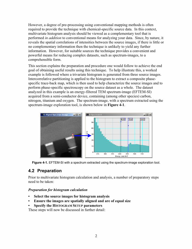
This section explains the preparation and procedure one would follow to achieve the end goal of obtaining useful results using this technique. To help illustrate this, a worked example is followed where a trivariate histogram is generated from three source images. Intercorrelative partitioning is applied to the histogram to extract a composite phase-specific trace-back map, which is then used to help characterize the source images and to perform phase-specific spectroscopy on the source dataset as a whole. The dataset analyzed in this example is an energy-filtered TEM spectrum-image (EFTEM-SI) acquired from a semi-conductor device, containing (among other species) carbon, nitrogen, titanium and oxygen. The spectrum-image, with a spectrum extracted using the spectrum-image exploration tool, is shown below in Figure 4-1.

Figure 4-1. EFTEM-SI with a spectrum extracted using the spectrum-image exploration tool.

4.2 Preparation Prior to multivariate histogram calculation and analysis, a number of preparatory steps need to be taken:

Preparation for histogram calculation

• Select the source images for histogram analysis • Ensure the images are spatially aligned and are of equal size • Specify the HISTOGRAM SETUP parameters These steps will now be discussed in further detail:

3

1. Selecting the source images. Appropriate source images need to be selected for histogram analysis. Two images are required for bivariate histogram analysis, and three for a trivariate histogram. The origins of the images themselves are not important; typically, EFTEM maps extracted from the same region may be used, or maps extracted from an EELS / EFTEM spectrum-image dataset are ideal. The fundamental criterion is that the images should contain spatially complementary information, although of course it is by applying the histogram analysis procedure itself that such a relationship is revealed. To this extent, even though chemical maps are recommended primarily for use with these routines, the histogram analysis tools can be used to investigate the spatial correlation between any complementary images (e.g. between thickness and SNR maps, bright and dark-field images, etc.). Hence it is difficult to recommend which image types are best suited to the technique, although of course data with a higher SNR will yield more satisfactory results, and images with well defined region specific information will give rise to better defined clusters of intensity within the generated histogram.

The three maps extracted from the EFTEM-SI, and used as the source images for the trivariate histogram analysis example referred to throughout this section, are shown in Figure 4-2. The chemical maps were calculated from the spectrum-image using the jump-ratio method over the C K, Ti L23 and O K ionization edges. As can be seen, the images contain a high degree of complementary information and as a result should give rise to well defined clusters in the generated histogram.

Figure 4-2. The carbon, titanium and oxygen jump-ratio maps used as source images in the

histogram analysis example.

2. Preparing the source images It is important to ensure the histogram source images are spatially aligned since the histogram analysis explores the spatial correlation of the images and hence any image misalignment will affect the accuracy of the histogram plot. Before extracting the chemical maps shown in Figure 4-2, the spatial drift between consecutive image acquisitions within the series was removed using the EFTEM-SI drift removal algorithm. Correction of spatial drift is not of concern for maps extracted from spectrum-images acquired using scanning techniques since the drift component will contribute to all extracted maps equally (i.e. the drift component will be spatially correlated). In addition,

4

the images should also be of equal size in the x and y directions; if this is not the case then crop the images to a common size ensuring they remain spatially aligned.

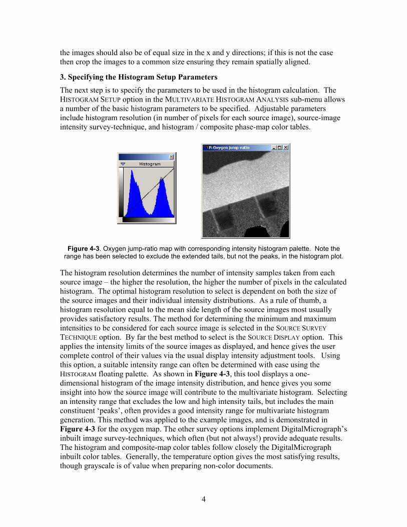
3. Specifying the Histogram Setup Parameters The next step is to specify the parameters to be used in the histogram calculation. The HISTOGRAM SETUP option in the MULTIVARIATE HISTOGRAM ANALYSIS sub-menu allows a number of the basic histogram parameters to be specified. Adjustable parameters include histogram resolution (in number of pixels for each source image), source-image intensity survey-technique, and histogram / composite phase-map color tables.

Figure 4-3. Oxygen jump-ratio map with corresponding intensity histogram palette. Note the range has been selected to exclude the extended tails, but not the peaks, in the histogram plot.

The histogram resolution determines the number of intensity samples taken from each source image – the higher the resolution, the higher the number of pixels in the calculated histogram. The optimal histogram resolution to select is dependent on both the size of the source images and their individual intensity distributions. As a rule of thumb, a histogram resolution equal to the mean side length of the source images most usually provides satisfactory results. The method for determining the minimum and maximum intensities to be considered for each source image is selected in the SOURCE SURVEY TECHNIQUE option. By far the best method to select is the SOURCE DISPLAY option. This applies the intensity limits of the source images as displayed, and hence gives the user complete control of their values via the usual display intensity adjustment tools. Using this option, a suitable intensity range can often be determined with ease using the HISTOGRAM floating palette. As shown in Figure 4-3, this tool displays a one-dimensional histogram of the image intensity distribution, and hence gives you some insight into how the source image will contribute to the multivariate histogram. Selecting an intensity range that excludes the low and high intensity tails, but includes the main constituent ‘peaks’, often provides a good intensity range for multivariate histogram generation. This method was applied to the example images, and is demonstrated in Figure 4-3 for the oxygen map. The other survey options implement DigitalMicrograph’s inbuilt image survey-techniques, which often (but not always!) provide adequate results. The histogram and composite-map color tables follow closely the DigitalMicrograph inbuilt color tables. Generally, the temperature option gives the most satisfying results, though grayscale is of value when preparing non-color documents.

5

4.3 Generating a Histogram Once the HISTOGRAM SETUP parameters have been specified, you can proceed with generating your multivariate histogram. If you have selected the SOURCE DISPLAY option for the SOURCE SURVEY TECHNIQUE, you should first define the intensity range of the source images before continuing.

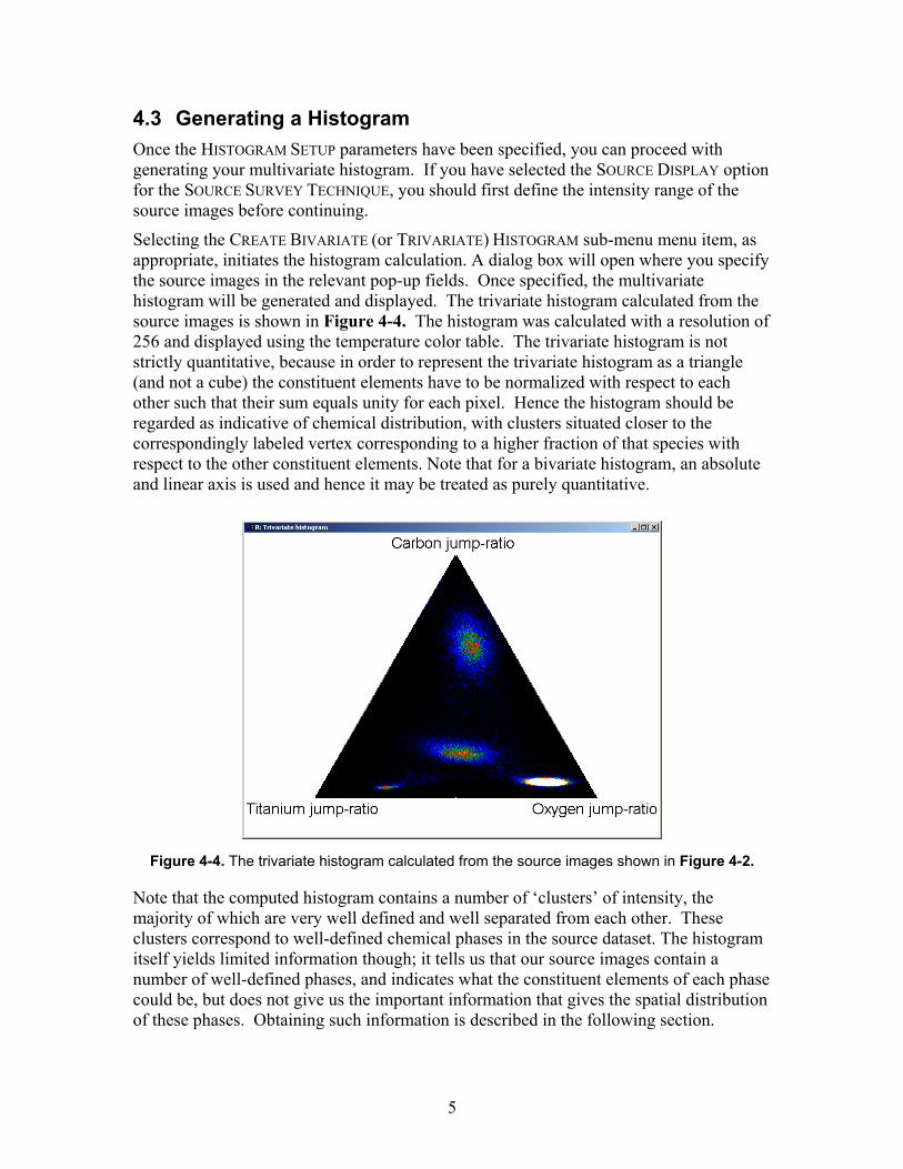
Selecting the CREATE BIVARIATE (or TRIVARIATE) HISTOGRAM sub-menu menu item, as appropriate, initiates the histogram calculation. A dialog box will open where you specify the source images in the relevant pop-up fields. Once specified, the multivariate histogram will be generated and displayed. The trivariate histogram calculated from the source images is shown in Figure 4-4. The histogram was calculated with a resolution of 256 and displayed using the temperature color table. The trivariate histogram is not strictly quantitative, because in order to represent the trivariate histogram as a triangle (and not a cube) the constituent elements have to be normalized with respect to each other such that their sum equals unity for each pixel. Hence the histogram should be regarded as indicative of chemical distribution, with clusters situated closer to the correspondingly labeled vertex corresponding to a higher fraction of that species with respect to the other constituent elements. Note that for a bivariate histogram, an absolute and linear axis is used and hence it may be treated as purely quantitative.

Figure 4-4. The trivariate histogram calculated from the source images shown in Figure 4-2.

Note that the computed histogram contains a number of ‘clusters’ of intensity, the majority of which are very well defined and well separated from each other. These clusters correspond to well-defined chemical phases in the source dataset. The histogram itself yields limited information though; it tells us that our source images contain a number of well-defined phases, and indicates what the constituent elements of each phase could be, but does not give us the important information that gives the spatial distribution of these phases. Obtaining such information is described in the following section.

6

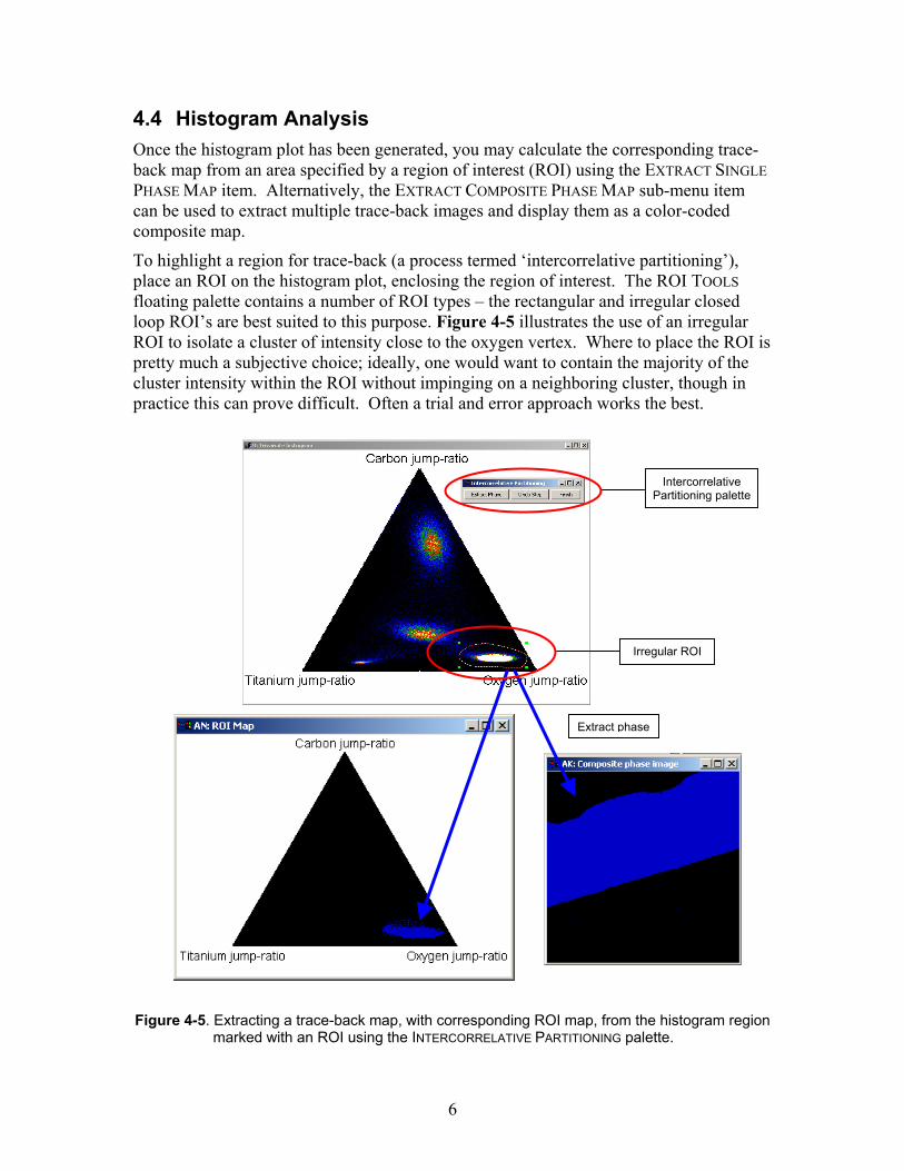
4.4 Histogram Analysis Once the histogram plot has been generated, you may calculate the corresponding trace-back map from an area specified by a region of interest (ROI) using the EXTRACT SINGLE PHASE MAP item. Alternatively, the EXTRACT COMPOSITE PHASE MAP sub-menu item can be used to extract multiple trace-back images and display them as a color-coded composite map.

To highlight a region for trace-back (a process termed ‘intercorrelative partitioning’), place an ROI on the histogram plot, enclosing the region of interest. The ROI TOOLS floating palette contains a number of ROI types – the rectangular and irregular closed loop ROI’s are best suited to this purpose. Figure 4-5 illustrates the use of an irregular ROI to isolate a cluster of intensity close to the oxygen vertex. Where to place the ROI is pretty much a subjective choice; ideally, one would want to contain the majority of the cluster intensity within the ROI without impinging on a neighboring cluster, though in practice this can prove difficult. Often a trial and error approach works the best.

Figure 4-5. Extracting a trace-back map, with corresponding ROI map, from the histogram region

marked with an ROI using the INTERCORRELATIVE PARTITIONING palette.

Extract phase

Irregular ROI

Intercorrelative Partitioning palette

7

Once the ROI is positioned to your satisfaction, a single trace-back map can be calculated by selecting the EXTRACT SINGLE PHASE IMAGE sub-menu item. The trace-back image will be calculated and displayed in a new image-window. Alternatively, one or more trace-back images may be computed and displayed as a composite image be selecting the EXTRACT COMPOSITE PHASE MAP option, as illustrated in Figure 4-5. Selecting this option launches the INTERCORRELATIVE PARTITIONING floating palette, which contains three buttons. The EXTRACT PHASE button calculates the trace-back image for the selected ROI. The extracted image is displayed in a new image-display, color-coded using the color-table as specified in the HISTOGRAM SETUP options (see Figure 4-5). After calculating the extracted phase-map, the contributing pixels within the histogram plot are removed temporarily to avoid inclusion to successive maps, and an ROI map is also displayed to indicate from where on the histogram the correspondingly color-coded trace-back maps have been extracted. After extraction, you may select a new region from the histogram and extract another phase-map. Successive phase maps are added to the same image-display, allowing a composite map to be gradually built-up. If you make a mistake, selecting the UNDO STEP button undoes the last calculation. When you are happy with your extracted composite trace-back map, select FINISH to close the floating palette and restore the source histogram to its initial state.

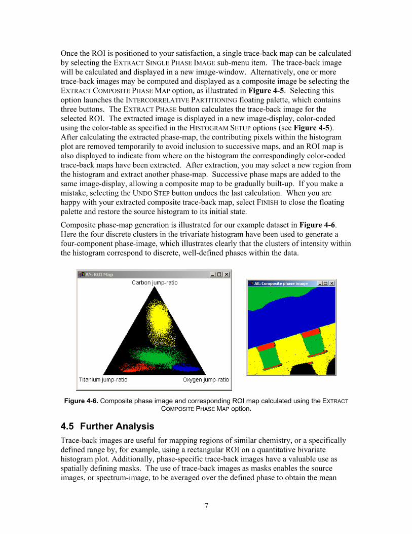
Composite phase-map generation is illustrated for our example dataset in Figure 4-6. Here the four discrete clusters in the trivariate histogram have been used to generate a four-component phase-image, which illustrates clearly that the clusters of intensity within the histogram correspond to discrete, well-defined phases within the data.

Figure 4-6. Composite phase image and corresponding ROI map calculated using the EXTRACT

COMPOSITE PHASE MAP option.

4.5 Further Analysis Trace-back images are useful for mapping regions of similar chemistry, or a specifically defined range by, for example, using a rectangular ROI on a quantitative bivariate histogram plot. Additionally, phase-specific trace-back images have a valuable use as spatially defining masks. The use of trace-back images as masks enables the source images, or spectrum-image, to be averaged over the defined phase to obtain the mean

8

counts per element for that phase in the case of elemental maps, useful for accurately determining atomic ratios, or alternatively for obtaining a phase-integrated spectrum from a spectrum-image data-set, an approach which enables phases to be characterized with high accuracy and optimized statistics. These two examples will now be illustrated.

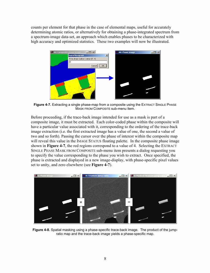
Figure 4-7. Extracting a single phase-map from a composite using the EXTRACT SINGLE PHASE

MASK FROM COMPOSITE sub-menu item.

Before proceeding, if the trace-back image intended for use as a mask is part of a composite image, it must be extracted. Each color-coded phase within the composite will have a particular value associated with it, corresponding to the ordering of the trace-back image extraction (i.e. the first extracted image has a value of one, the second a value of two and so forth). Passing the cursor over the phase of interest within the composite map will reveal this value in the IMAGE STATUS floating palette. In the composite phase image shown in Figure 4-7, the red regions correspond to a value of 4. Selecting the EXTRACT SINGLE PHASE MASK FROM COMPOSITE sub-menu item presents a dialog requesting you to specify the value corresponding to the phase you wish to extract. Once specified, the phase is extracted and displayed in a new image-display, with phase-specific pixel values set to unity, and zero elsewhere (see Figure 4-7).

Figure 4-8. Spatial masking using a phase-specific trace-back image. The product of the jump-

ratio map and the trace-back image yields a phase-specific map.

× =

9

To apply a mask to a single image, simply calculate the product of the two images using the SIMPLE MATH... option in the PROCESS menu. This is illustrated in Figure 4-8, where the trace-back image corresponding to the red-phase (which, judging from the ROI map in Figure 4-6, is most probably titanium rich) is used to mask the titanium jump-ratio map. Using the SUM item in the STATISTICS sub-menu, found in the ANALYSIS menu, the total number of non-zero pixels in the phase-specific trace-back image is 2031 (i.e. the sum of the trace-back image), and the sum of the masked Ti jump-ratio image is 2927. Hence the mean Ti jump-ratio for the regions specified by the mask is 1.44. Similarly, the mean C and O jump-ratios in the region defined by the mask are calculated as 0.66 and 0.89 respectively. This simple example illustrates the usefulness of phase-specific trace-back masks in obtaining mean values from phase-specific regions.

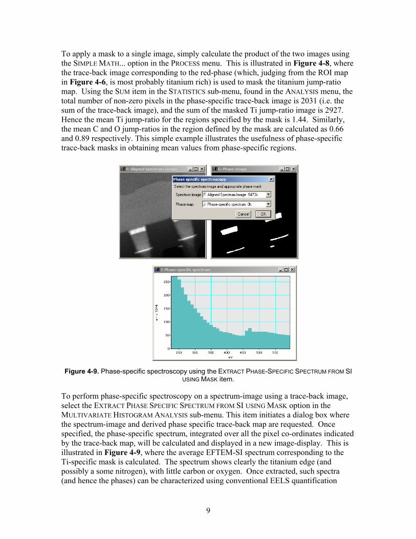
Figure 4-9. Phase-specific spectroscopy using the EXTRACT PHASE-SPECIFIC SPECTRUM FROM SI

USING MASK item.

To perform phase-specific spectroscopy on a spectrum-image using a trace-back image, select the EXTRACT PHASE SPECIFIC SPECTRUM FROM SI USING MASK option in the MULTIVARIATE HISTOGRAM ANALYSIS sub-menu. This item initiates a dialog box where the spectrum-image and derived phase specific trace-back map are requested. Once specified, the phase-specific spectrum, integrated over all the pixel co-ordinates indicated by the trace-back map, will be calculated and displayed in a new image-display. This is illustrated in Figure 4-9, where the average EFTEM-SI spectrum corresponding to the Ti-specific mask is calculated. The spectrum shows clearly the titanium edge (and possibly a some nitrogen), with little carbon or oxygen. Once extracted, such spectra (and hence the phases) can be characterized using conventional EELS quantification

10

techniques, with counting statistics optimized since the spectra have been summed over all the pixels present within the identified phase.

11

5 Quick Reference to Multivariate Histogram Analysis To create a multivariate histogram

1. Ensure the source images are of similar size and are spatially aligned.

2. Enter the desired options in the histogram setup dialog initiated by selecting the HISTOGRAM SETUP… sub-menu item.

3. If the Source Display survey technique was selected, specify the maximum and minimum intensity levels by either highlighting the desired range using the Histogram floating window, or by entering the values directly in the appropriate fields via the IMAGE DISPLAY… dialog.

4. Select CREATE BIVARIATE (or TRIVARIATE) HISTOGRAM, and specify the source images in the pop-up menu dialog.

5. The bivariate histogram will be calculated and displayed in a new image window. If the displayed intensity range is not to your liking, repeat steps 2-4 using a different survey range or technique.

To extract a single phase map from a multivariate histogram plot

1. Highlight the region of interest on the histogram plot using an ROI tool.

2. Select the EXTRACT SINGLE PHASE IMAGE item.

To extract a composite phase map from a multivariate histogram plot

1. Specify the desired color table in the COMPOSITE PHASEMAP COLOR TABLE pull down menu in the HISTOGRAM SETUP… dialog.

2. With the multivariate histogram front-most, select EXTRACT COMPOSITE PHASE to initiate the INTERCORRELATIVE PARTITIONING floating palette.

2. Select the histogram region of interest an ROI tool, and select EXTRACT PHASE on the floating palette to extract the phase and ROI maps.

3. Repeat step 3 to add additional phase maps. Undo steps using UNDO STEP on the floating palette.

4. When complete, select FINISH.

To extract a single phase image from a composite phase map

1. With the multivariate histogram front-most, select EXTRACT SINGLE PHASE MAP.

2. Enter the corresponding number (i.e. the pixel value) of the phase you wish to extract.

To extract a phase-specific spectrum from a spectrum-image using a phase-map

1. Select EXTRACT PHASE-SPECIFIC SPECTRUM FROM SI USING MASK.

2. Specify the spectrum-image and (single) phase image in the appropriate fields.