Multivariate strategies in functional magnetic

resonance imaging

Lars Kai Hansen

Informatics and Mathematical Modelling,Technical University of Denmark,DK-2800 Kgs. Lyngby, Denmark

Abstract

We discuss aspects of multivariate fMRI modeling, including the statistical evalua-tion of multivariate models and means for dimensional reduction. In a case study weanalyze linear and non-linear dimensional reduction tools in the context of a ‘mindreading’ predictive multivariate fMRI model.

Key words: Generalization, dimensional reduction, Laplacian eigenmap, NPAIRS,fMRI

Introduction

The human brain processes information in a massively parallel network ofhighly interconnected neuronal ensembles. In order to understand the resultinglong range spatio-temporal correlations in functional image sets, we and othershave pursued a wide variety of multivariate analysis strategies. To reducethe two important sources of bias in neuroimage analysis, namely model biasand the statistical bias arising from relatively small sample sizes available formodeling.

Neuroimaging experiments are designed to explore the spatio-temporal patternof information processing in the brain associated with a given behavior ordelivery of stimulus. Stimuli may be external, e.g., passive viewing, hearingetc., or may be internally generated by spontaneous cognitive processes orphysical activity, e.g., speaking, motor activity; for a review see (Frackowiaket al., 2003). The brain imaging device measures the mesoscopic brain state,

Email address: lkh@imm.dtu.dk (Lars Kai Hansen).

Preprint submitted to Elsevier Science 16 May 2006

i.e., information processing averaged over small volumes, called voxels. Wedenote this high-dimensional image measurement by x(t), with t being thetime of acquisition. The corresponding macroscopic cognitive state is denotedby g(t). The total amount of data is denoted D = (xt,gt, )t = 1, ..., T .

Thus, the neuroimaging agenda is to explore the joint distribution: p(x,g)based on D and background neuroinformatics knowledge bases.

The joint distribution of brain states and behavior can be modelled directly, oras more frequently done by one of the two equivalent factorizations: p(x,g) =p(x|g)p(g) or p(x,g) = p(g|x)p(x).

By factoring p(x,g) = p(x|g)p(g), we consider the stimulus as the controlsignal and look for differences in the neuroimage distribution among differentcognitive states. This is the most prevalent mode of analysis, dating backto the so-called subtraction paradigm, in which the mean images from twodifferent conditions are subtracted and shown as a measure of contrast. Thisapproach has been refined in the several neuroimage analysis tools, e.g., SPM,see (Frackowiak et al., 2003). In SPM the conditional neuroimage distributionis further factorized as p(x|g) ∼ ∏

i p(xi|g), where xi are individual voxelmeasurements. A product of such univariate factors amounts is equivalent toassuming voxel-to-voxel independence, also known as ‘naıve Bayes’. Further,by assuming that the univariate conditionals are all Gaussian distributionswe arrive at the generative model equivalent to SPM’s mass univariate t-testapproach, framed in the so-called general linear model, see also (Kjems et al.,2002) for further discussions of the naive Bayes generative model.

On the other hand by factoring the joint pdf as p(x,g) = p(g|x)p(x), we enterwas has been dubbed the mind reading paradigm, in which the model is setup to infer the instantaneous cognitive state from the concurrent neuroimage.This approach was first developed by in the mid-90s (Lautrup et al., 1994;Mørch et al., 1995, 1997) for functional neuroimaging based on PET and fMRI,and has also more recently gained interest in the machine learning community,see e.g., (Mitchell et al., 2004). As a historical note: the first application ofartificial neural networks for classifications of brain scans date back to the1992 (Kippenham et al., 1992), and concerned the classification of regionallyaveraged PET data in terms of normal and Alzheimers disease. Univariate andmultivariate models including: SPM, cross-correlation analysis, independencomponent analysis, artificial neural networks, were carefully compared usingboth simulate and real data in the 1999 NeuroImage paper by (Lange et al.,1999).

2

Predictive value: The generalizability of a model

We model probability distributions (countable support) or probability den-sity functions (continuous support) using parameterized families, p(x,g) ∼p(g,x|θ), where the parameters θ can be both continuous (like means andvariances) or discrete (like model orders, number of components, etc.). A neu-roimaging experiment is not able to pin down the parameters, rather we are leftwith an uncertainty captured by the so-called posterior distribution p(θ|D).Given the posterior distribution we may predict or simulate future data basedon the initial data

p(xt+1,gt+1|D) =∫

p(xt+1,gt+1|θ)p(θ|D)dθ, (1)

The closer these predictions are to ‘true’ pdf’s: p(xt+1,gt+1), the more gener-alizable the model is, i.e., the more similar are the two stochastic processes.Closeness may be measured by one of several costfunctions. Often used cost-functions are the miss-classification rate, the mean square error, and the de-viance (Ripley, 1996). The generalization error is defined as the expected coston a new datum.

The expected deviance is - apart from a an additive constant - identical to thebasic information theoretic Kullback-Leibler measure,

KL[p(.), p(.|D)] =∫ ∫

log

[p(x,g)

p(x,g|D)

]p(x,g)dxdg (2)

This loss is zero if the predictive distribution is identical to the ‘true’ distribu-tion and otherwise positive for all other distributions. The generalization errordifference between two models may be estimated by a sample of test data

∆KL = KL[p(.), p1(.|D)]− KL[p(.), p2(.|D)] =1

Ttest

Ttest∑

τ=1

log

[p2(xτ ,gτ |D)

p1(xτ ,gτ |D)

]

(3)This test error is an unbiased estimate of the generalization error if the testset is sampled independently from the training data D.

The generalization error typically depends strongly on the amount data in thetraining set N = |D|, and is also strongly dependent on the complexity of themodel. Most often the generalization error decreases as a function of N , hencethe models generalize better the more data is provided. If the model family canbe described by a single complexity parameter, say the number of estimatedparameters, there is typically a bias-variance trade-off: The best model is nottoo simple (biased) and not too complex. If the model is too complex thepredictive distribution will be able to adapt to closely to the training data,hence, be highly too different between different training sets (variance).

3

Hence, one could say that there is always a hidden agenda in modeling fromdata: We are interested in models that predict well, not simply models thatfit well to the training data.

It can be shown that for the deviance loss function the optimal predictivedistribution is obtained using so-called Bayesian averaging,

p(θ|D) =p(D|θ)p(θ)∫p(D|θ)p(θ)dθ

, (4)

where p(D|θ) is the likelihood function, and p(θ) is the ‘true’ prior distribution.In practise the true prior is not available and most often the likelihood is atbest an approximation to the true likelihood. However, it is an empirical find-ing that even rather crude approximate Bayesian averaging procedures providebetter predictive distributions than that obtained from using a point estimate,e.g., a maximum likelihood estimate p(.) ∼ p(.|θML(D)), where θML(D) maxi-mize the likelihood function. The main difficulty with the Bayesian estimatorsis the often significant computational overheads incurred by parameter aver-aging. Note that the generalization error and the unbiased estimate can beused to evaluate any model, no matter how the models predictive distributionis obtained.

In neuroimaging we are interested in models that generalize and models thatcan be interpreted, typically in terms of a ‘brain map’: an image or volume oflocal activation involvement, i.e., a statistical parametric map. For multivari-ate neuroimaging models of the SPM is a function of the model parameters,hence, we are interested in a models for which the parameters are relativelyrobust.

To investigate the stability of representations we have suggested the NPAIRSframework. NPAIRS is based on split half resampling. For two models adaptedto fit two independently sampled data subsets of the same size, i.e., the twosets in split half, any derived parameters should be identical between the twosubsets. Thus the difference between SPMs estimated in the two sets is anunbiased estimator of the pixel-by-pixel variance. For additional discussionand examples see (Kjems et al., 2002; Strother et al., 2002). Other resamplingstrategies may under different assumption provide useful estimators, e.g., boot-strap and jackknife which is closely related to leave-one-out cross-validation,see e.g., (Kjems et al., 2000). In our analysis below we are primarily inter-ested in the predictive value of the models, hence, we use the leave-one-outfor estimation of performance.

4

Models

We characterize models as parametric, non-parametric, and semi-parametric(Bishop, 1995). Parametric models have fixed parameter sets, say mean andco-variance for a normal pdf model. Non-parametric models use the data setas model, e.g., nearest neighbor density models. Semi-parametric models havea general structure but with variable dimensionality of the parameterization,e.g., mixture models where the number of mixture components is determinedfrom data. Examples of parametric models cover, e.g, modelling with nor-mal distributions. The normal distribution is described by the mean vectorand the co-variance matrix. Gaussian mixture models (clustering) and artifi-cial neural networks are typical semi-parametric systems (Bishop, 1995). Theparametrizations are adapted to the given data set. Nearest neighbor meth-ods are generic non-parametric models. Non-parametric models are extremelyflexible and need careful complexity control.

In machine learning a further distinction is made between supervised andunsupervised learning. In supervised learning the aim is to model conditionaldistributions, e.g., p(g|x). To adapt models we need supervised data sets withboth inputs x) and outputs g. In unsupervised learning we are interested inmodeling marginal pdf’s, e.g., p(x), which can be adapted from a sample of‘input’ data only (Mørch et al., 1997).

Dimensionality reduction

Data sets of neuroimages usually have many more voxels J than image samples(T << J). This means that multivariate models involving the image repre-sentation can easily be ill-posed. If, e.g., a parameter is used for each imagedimension we would thus invoke at least J parameters, which would be esti-mated on T samples. Thus, we need to consider the representation carefullyfor example by an initial dimensional reduction step prior to modeling.

The primary objective of dimensional reduction is to create a mapping fromthe original high dimensional image space to a relevant low dimensional sub-space in which we can safely establish the posterior distribution. Principalcomponent analysis (PCA) is a well established scheme for dimension reduc-tion in functional imaging, see e.g., the discussions in (Kjems et al., 2000, 2002;Strother et al., 2002). PCA identifies an orthogonal basis for a subspace whichcaptures the most variance for a given dimensionality. Dimensional reductionusing PCA is meaningful if the dominant effects in the data are those in-duced by the stimulus. More advanced representations based linear projectionschemes, some of which are further including information from the reference

5

function are discussed in (Worsley et al., 1997).

It is worth noting that the PCA approach is not jeopardized if the data con-tains high variance, confounding signal components because these can be sup-pressed in the subsequent modeling; the requirement is that the effects ofinterest are present in the subspace. We will therefore be quite liberal in ourchoice of subspace dimension in the following. PCA is achieved by singularvalue decomposition (SVD), see e.g. (Kjems et al., 2000). The data matrix Dof size J × T where T ¿ J , is decomposed into

D = USV>, (5)

where U is a J × T orthonormal matrix, S is a T × T diagonal matrix and Vis T × T orthonormal matrix using a so-called ‘economy size’ decompositionwhere the null space has been removed. The diagonal of matrix S has nonneg-ative elements in descending order. These diagonal elements are the singularvalues that correspond to standard deviations of the input data projected ontothe given basis vectors represented by matrix U. The reduced input space isobtained by using only some fixed K ≤ N number of the largest principalcomponents. The reduced data matrix is given by

X = U>D, (6)

where the transformation matrix from the original input space to the reducedinputs space is given by U, a F × K sub-matrix of U. Here we use the factthat U is orthonormal giving U−1 = U>.

Our focus here is on the prediction and reproducibility performance of models.We will invoke a resampling (cross-validation) scheme. Thus we need to enforcethat not only the classifier is generalizable, but also the reduced representation.Using all the data to estimate the transformation matrix U would introducedependence between the training set and test set. To avoid this dependence,the PCA is computed using only training data, giving a U transformationmatrix. This matrix is then used to transform the test data to the lowerdimensional subspace with

Xte = U>Dte, (7)

which ensures the unbiased nature of the test data. Tools exist for optimizingthe PCA signal-to-noise ratio, with respect to the dimensionality K (Hansenet al., 1999; Beckmann et al., 2001).

Linear dimension reduction can be based on more advanced decompositions,such as independent component analysis (ICA) (McKeown et al., 2003). Theadvantage of ICA is that is not subject to the strong orthogonality constraintsof PCA, which means that it can eliminate more subtle artifacts than PCA.For relatively high-dimensional mappings the difference in subspaces spanned

6

by the orthogonal basis by PCA and the non-orthogonal basis of ICA is notlikely to be of much significance.

Non-linear dimensional reduction has not been explored nearly as widely astheir linear counterparts. (Thirion and Faugeras, 2004) investigated so-calledLaplacian eigenmaps (Belkin and Niyogi, 2002) as a dimensional tool, thesemaps are created as non-linear low-dimensional representations that as closelyas possible maintains the topological neighbors in a high-dimensional fea-ture space, similar in spirit to the classical multi-dimensional scaling method(Kruskal and Wish, 1978).

The Laplacian eigenmap is based on a non-Euclidean metric, defined thougha kernel function

d(j, k) = K(xj − xk) (8)

In many applications the kernel is chosen to be the gaussian function K(u) =exp(−u2/σ2). Based on the metric the N ×N matrix Q is established as thematrix of pairwise distances between data points. Let rj be the j′th row sum ofQ, and let R be the diagonal matrix with vector r in the diagonal. The Laplaceeigenmaps are the N -dimensional eigenvectors of matrix Q−R. The Laplaceeigenmap is closely related to so-called spectral clustering (Weiss, 1999), andthe interpretation is similar. Two data points are active in a given Laplaceeigenmap if there is a ‘diffusion path’ between the two formed by neighboringdata points active in the given map. While linear dimensional reduction basedon variance can be expected to work well for modelling strong mean differenceeffects, the Laplacian eigenmap can form a representation in which warpedmean effects are present, say in the presence of a weak non-stationarity ordrift of the class means so that they form non-linear trajectories in inputspace, say as function of time, see e.g., (Ng et al., 2001) for several creativeillustrations.

Case Study

The data set used for illustration of multivariate models in this presentationwas acquired by dr. Egill Rostrup at Hvidovre Hospital on a 1.5 T MagnetomVision MR scanner. The scanning sequence was a 2D gradient echo EPI (T2∗weighted) with 66 ms echo time and 50 degrees RF flip angle. The images wereacquired with a matrix of 128× 128 pixels, with FOV of 230mm, and 10mmslice thickness, in a para-axial orientation parallel to the calcarine sulcus. Thevisual paradigm consisted of a rest period of 20sec of darkness using a lightfixation dot, followed by 10sec of full-field checkerboard reversing at 8Hz,and ending with 20sec of rest (darkness). In total, 150 images were acquiredin 50sec, corresponding to a period of approximately 330msec per image. Theexperiment was repeated in 10 separate runs containing 150 images each. In

7

order to reduce saturation effects, the first 29 images were discarded, leaving121 images for each run.

Representations

Based on the 1210 scans included in the analysis we form a linear princi-pal component representation and a nonlinear representation based on theLaplacian eigenmaps. The topology of the two representations are illustratedin Figure and Figure respectively. The linear representation shows a pro-nounced mean difference effect between baseline and activation scans, whilethe non-linear representation is somewhat more subtle showing difference inthe shape of the clusters of baseline and activation scans, revealing potentialnon-stationarity in the two states.

[Figure 1 here]

[Figure 2 here]

Non-parametric modeling

The next step in modeling is to construct a map representing the relation be-tween brain image and brain state. This have been accomplished using bothparametric models, e.g., (Kjems et al., 2002), semi-parametric (Mørch et al.,1997), and non-parametric models e.g. (Mitchell et al., 2003). We here followthe latter and use the k-nearest neighbor model (KNN). This system is typi-cally computing neighbors using an un-weighted Euclidean metric in featurespace, and most often classifying by majority voting among the neighbors.It remains to determine the number of neighbors k. We use a leave-one-outresampling scheme in the training set to select k. This can be done a very lit-tle overhead. The leave-one-out error can simply be computed by classifyingusing the neighbors excluding the actual data point. The optimal k can thenbe used in classifying the training set. If a full Bayes posterior probability isrequired, the method is easily extended to compute local pdf values (Bishop,1995).

We use both PCA and Laplacian eigenmap features to illustrate the procedure.We split the dataset in two equal size subsets: Five runs for training andfive runs for testing. As the test and training data are independent, the testerror estimates are unbiased estimator of performance. We use a simple on-off activation reference function for supervision of the classifier. The referencefunction is off-set by 4 seconds to emulate the hemodynamic delay.

8

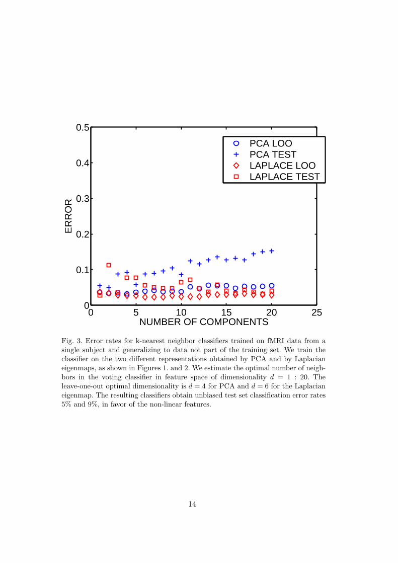
For each method we estimate k for a number of feature space dimensionsd = 1 : 20 using the leave-one-out (LOO) procedure on the training set. TheLOO-optimal k is then applied to the test set for the same feature spacedimensionality and a classification error rate estimated on the test set, theresulting relations between feature space dimensionality, LOO and test errorsare indicated in Figure 3. The best (LOO) error is obtained for a d = 6dimensional feature subspace for the Laplacian eigenmap, while the best modelusing PCA is a d = 4. The corresponding unbiased test set classification errorrates are 5% and 9%, in favor of the non-linear features.

[Figure 3 here]

[Figure 4 here]

In Figure 4. we show the test set activation time series obtained by the twomodels. In the non-linear feature the errors basically occurs at the onset andat end of stimulation, while the PCA based linear feature representations alsomake generalization errors in the baseline, suggesting spurious short burst ofactivation.

Discussion

For modeling of neuroimaging data we are in general interested in models thatare able to extract the relevant generalizable long range dependencies betweenbehavior and brain state, hence, that have predictive power. Because of thehigh-dimensional representations that are inherent in multivariate models weneed to exercise extreme care in model optimization. This includes dimen-sional reduction and feature selection. We have outlined a resampling basedapproach framework and demonstrated its implementation for general non-linear models including also non-linear dimensional reduction schemes. In avisual simulation study we have shown that non-linear dimensional reductionand non-parametric modeling led to optimal generalizability.

Acknowledgments

This work is supported Human Brain Project Grant P20 MN57180, and theDanish foundation Lundbeckfonden.

9

References

Beckmann, C., Noble, J., Smith, S., 2001. Investigating the intrinsic dimen-sionality of fmri data for ica. In: Proc. Seventh Int. Conf. on FunctionalMapping of the Human Brain. NeuroImage. p. 13(6)S76.

Belkin, M., Niyogi, P., 2002. Laplacian eigenmaps and spectral techniques forembedding and clustering.URL citeseer.ist.psu.edu/belkin01laplacian.html

Bishop, C., 1995. Neural Networks for Pattern Recognition. Oxford UniversityPress, Oxford.

Frackowiak, R., Friston, K., Frith, C., Dolan, R., Price, C., Zeki, S., Ashburner,J., Penny, W. (Eds.), 2003. Human Brain Function, 2nd Edition. AcademicPress.URL http://www.fil.ion.ucl.ac.uk/spm/doc/books/hbf2/

Hansen, L., Paulson, O., Larsen, J., Nielsen, F., Strother, S., Rostrup, E.,Savoy, R., Lange, N., Sidtis, J., Svarer, C., 1999. Generalizable Patterns inNeuroimaging: How Many Principal Components? NeuroImage 9, 534–544.

Kippenham, J., Barker, W., Pascal, S., Nagel, J., Duara, R., 1992. Evalua-tion of a neural network classifier for PET scans of normal and AlzheimersDisease Subjects. Journal Nuclear Medicine 33, 1459–1467.

Kjems, U., Hansen, L., Anderson, J., Frutiger, S., Muley, S., Sidtis, J., Rotten-berg, D., Strother, S., 2002. The Quantitative Evaluation of Functional Neu-roimaging Experiments: Mutual Information Learning Curves. NeuroImage15 (4), 772–786.

Kjems, U., Hansen, L. K., Strother, S. C., 2000. Generalizable singular valuedecomposition for ill-posed datasets. In: NIPS. pp. 549–555.

Kruskal, J. B., Wish, M., 1978. Multidimensional Scaling. Sage Publications,Beverly Hills, California.

Lange, N., Strother, S. C., Anderson, J. R., Nielsen, F. A., Holmes, A. P.,Kolenda, T., Savoy, R., Hansen, L. K., September 1999. Plurality andresemblance in fMRI data analysis. NeuroImage 10 (3), 282–303.URL http://www.sciencedirect.com/science/article-

/B6WNP-45FCP48-13/2/bd7e7f72099b83540609e24c627a2fc4

Lautrup, B., Hansen, L., Law, I., Mørch, N., Svarer, C., Strother:, S., 1994.Massive Weight Sharing: A cure for Extremely Ill-posed Problems. In: Work-shop on Supercomputing in Brain Research: From Tomography to NeuralNetworks. Juelich, Germany, pp. 137–144.

McKeown, M., Hansen, L. K., Sejnowski, T. J., oct 2003. Independent compo-nent analysis for fmri: What is signal and what is noise? Current Opinionin Neurobiology 13 (5), 620–629.URL http://www2.imm.dtu.dk/pubdb/p.php?2878

Mitchell, T., Hutchinson, R., abd R.S. Niculescu, M. J., Pereira, F., Wang, X.,2003. Classifying instantaneous cognitive states from fmri data. In: Ameri-can Medical Informatics Association Annual Symposium.

Mitchell, T., Hutchinson, R., Niculescu, R., Pereira, F., Wang, X., Just, M.,

10

Newman, S., 2004. Learning to Decode Cognitive States from Brain Images.Machine Learning 57 (1).

Mørch, N., Hansen, L., Strother, S., Svarer, C., Rottenberg, D., Lautrup, B.,Savoy, R., Paulson, O., 1997. Nonlinear versus Linear Models in FunctionalNeuroimaging: Learning Curves and Generalization Crossover. In: Proceed-ings of the 15th International Conference on Information Processing in Med-ical Imaging, 1997. Vol. Springer Lecture Notes in Computer Science 1230.pp. 259–270.

Mørch, N., Kjems, U., Hansen, L., Svarer, C., Law, I., Lautrup, B., Strother, S.,Rehm, K., 1995. Visualization of Neural Networks Using Saliency Maps. In:Proceedings of the 1995 IEEE International Conference on Neural Networks.Vol. 4. pp. 2085–2090.

Ng, A., Jordan, M., Weiss, Y., 2001. On spectral clustering: Analysis and analgorithm.URL citeseer.ist.psu.edu/ng01spectral.html

Ripley, B. D., 1996. Pattern Recognition and Neural Networks. CambridgeUniversity Press, Cambridge.

Strother, S., Anderson, J., Hansen, L., Kjems, U., Kustra, R., Sidtis, J.,Frutiger, S., Muley, S., LaConte, S., Rottenberg, D., 2002. The Quanti-tative Evaluation of Functional Neuroimaging Experiments: The NPAIRSData Analysis Framework. NeuroImage 15 (4), 747–771.

Thirion, B., Faugeras, O., Apr. 2004. Nonlinear dimension reduction of fM-RIdata: the Laplacian embedding approach. In: Proc. 2st Proc. IEEE ISBI.Arlington, VA, pp. 372–375.

Weiss, Y., 1999. Segmentation using eigenvectors: A unifying view. In: ICCV(2). pp. 975–982.URL citeseer.ist.psu.edu/weiss99segmentation.html

Worsley, K. J., Poline, J.-B., Friston, K. J., Evans, A. C., November 1997.Characterizing the response of PET and fMRI data using multivariate linearmodels. NeuroImage 6 (4), 305–319.URL http://www.idealibrary.com/links/citation/1053-8119/6/305

11

PC 1

PC 2

PC 3

PC 4

PC 5

Fig. 1. Linear representation by principal component analysis. The individual subgraphs show scatter plots of the indicated principal component projections of data.The data set consists of 1210 single BOLD fMRI slices (TR = 0.333 sec) acquiredin a para-axial orientation parallel to the calcarine sulcus. The subject was exposedvisual stimulation in a simple block design in ten runs (stimulated scans markedas red, baseline marked as blue). The representation is determined by linear pro-jections of maximum variance. The basis vectors are subject to strict orthogonalityconstraints. The baseline-activation difference is seen as a mean shift effect in severalscatter plots, e.g., PC1 vs PC2. The scatter plots below the diagonal are zoomedand rotated versions of the corresponding plots above the diagonal for illustrationof details in the representation.

12

LP 1

LP 2

LP 3

LP 4

LP 5

Fig. 2. Non-linear representation by Laplacian eigenmaps. The individual sub graphsshow scatter plots of the indicated eigenmap projections of data. The data set con-sists of 1210 single BOLD fMRI slices (TR = 0.333 sec) acquired in a para-axialorientation parallel to the calcarine sulcus. The subject was exposed visual stimula-tion in a simple block design in ten runs (stimulated scans marked as red, baselinemarked as blue). The projections are determined as eigenvectors of a neighbor diffu-sion matrix, hence, data is mapped together if there is a ‘short-hop path’ connectingvia neighbors active in the same map. The baseline-activation difference is seen hereas a projection shape difference as opposed to the mean shift effect of the linear PCAprojections illiustrated in Figure 1. As in Figure 1. the scatter plots below the di-agonal have been zoomed and rotated relative to the corresponding plots above thediagonal for illustration of details in the representation.

13

0 5 10 15 20 250

0.1

0.2

0.3

0.4

0.5

NUMBER OF COMPONENTS

ER

RO

R

PCA LOOPCA TESTLAPLACE LOOLAPLACE TEST

Fig. 3. Error rates for k-nearest neighbor classifiers trained on fMRI data from asingle subject and generalizing to data not part of the training set. We train theclassifier on the two different representations obtained by PCA and by Laplacianeigenmaps, as shown in Figures 1. and 2. We estimate the optimal number of neigh-bors in the voting classifier in feature space of dimensionality d = 1 : 20. Theleave-one-out optimal dimensionality is d = 4 for PCA and d = 6 for the Laplacianeigenmap. The resulting classifiers obtain unbiased test set classification error rates5% and 9%, in favor of the non-linear features.

14

100 200 300 400 500 600−4

−2

0

2

4

6

8Time−shifted stimulusKNN + Laplace reductionKNN + PCA reduction

Fig. 4. Test set reference activation time course and activation time courses producedby k-nearest neighbor classifiers based on linear and non-linear feature spaces. Thenon-linear feature based classifier’s errors basically occurs at the onset and at endof stimulation. The KNN model based on the linear feature representation makeadditional generalization errors in the baseline, where it suggest a few short burstof activation.

15