multivariate student- self-organizing maps

Neural Networks 22 (2009) 1432–1447

Contents lists available at ScienceDirect

Neural Networks

journal homepage: www.elsevier.com/locate/neunet

Multivariate Student-t self-organizing mapsEzequiel López-Rubio ∗Department of Computer Languages and Computer Science, University of Málaga, Bulevar Louis Pasteur, 35. 29071 Málaga, Spain

a r t i c l e i n f o

Article history:Received 3 October 2008Revised and accepted 1 May 2009

Keywords:Self-organizing mapsFinite mixture modelsMultivariate Student-t distributionsUnsupervised learningStochastic approximationAdaptive filteringClassification

a b s t r a c t

The original Kohonen’s Self-Organizing Map model has been extended by several authors to incorporatean underlying probability distribution. These proposals assume mixtures of Gaussian probabilitydensities. Here we present a new self-organizing model which is based on a mixture of multivariateStudent-t components. This improves the robustness of the map against outliers, while it includes theGaussians as a limit case. It is based on the stochastic approximation framework. The ‘degrees of freedom’parameter for each mixture component is estimated within the learning procedure. Hence it does notneed to be tuned manually. Experimental results are presented to show the behavior of our proposal inpresence of outliers, and its performance in adaptive filtering and classification problems.

© 2009 Elsevier Ltd. All rights reserved.

1. Introduction

The concept of self-organization seems to explain severalproperties of the brain that are linked to invariant feature detection(Fukushima, 1999). These properties inspired the proposal ofcomputational maps designed to explore multidimensional data,which have become pervasive in many fields of computationalintelligence. Typical applications include exploratory data analysis(Dittenbach, Rauber, &Merkl, 2002; Brugger, Bogdan, & Rosenstiel,2008), visualization of complex datasets (Kiang & Fisher, 2008;Prieto, Tricas, Merelo, Mora, & Prieto, 2008), clustering (Ciaramellaet al., 2008; Correa & Ludermir, 2008), classification (Chen, Tai,Wang, Deng, & Chen, 2008; Dokur & Ölmez, 2008) and content-based data retrieval (Laaksonen, Koskela, & Oja, 2002, 2004). Theoriginal self-organizing map (SOM) was proposed by Kohonen(1990), where each neuron has a weight vector to represent apoint of the input space. The neurons have disjoint activationregions, and no probability model is defined. Several approacheshave been proposed to overcome these limitations. The self-organizing map is defined as a mixture of Gaussian components,and the activation regions overlap. Among these proposals, theSelf-Organizing Mixture Model (SOMM) by Verbeek, Vlassis, andKrose (2005) uses a version of the expectation-maximization (EM)method to produce an extension of the SOM where a mixtureof restricted Gaussians is defined. Other families of probabilisticself-organizingmaps include kernel-based topographic maps (VanHulle, 2002a, 2002b, 2005), where Gaussian kernels are defined

∗ Tel.: +34 95 213 71 55; fax: +34 95 213 13 97.E-mail address: [email protected].

0893-6080/$ – see front matter© 2009 Elsevier Ltd. All rights reserved.doi:10.1016/j.neunet.2009.05.001

around a centroid. The aforementioned models consider onlydiagonal covariance matrices. This is not the case of the Self-Organizing Mixture Networks (SOMN), by Yin and Allinson (2001),which use full covariance Gaussians.Gaussianmixtures have attracted nearly all the attention in this

field because of their computational convenience. Nevertheless, formany real datasets the tails of the normal distribution are not aslong as the problem requires. This affects the estimation of themean vector and the covariance matrix, which can be ruined byatypical samples, also called outliers. As the dimension of the dataincreases, the problem gets harder to solve (Rocke & Woodruff,1997; Kosinski, 1999), in particular if the dataset is small, becausethe estimation of the covariance matrix under these conditions isan ill posed problem (Hoffbeck & Landgrebe, 1996; Bickel & Levina,2007). Hence, data analysis methods usually benefit from theintroduction of mixtures of multivariate Student-t distributions(Peel & McLachlan, 2000; Shoham, 2002; Svensén & Bishop, 2005;McLachlan, Bean, & Peel, 2002), since these distributions havelonger tails. Moreover, they include the mixtures of Gaussiansas a limit case. A recent proposal considers a fuzzy treatmentof these models, with applications to fuzzy clustering (Chatzis &Varvarigou, 2008). Finally, Principal Component Analysis (PCA) formixtures of Student-t distributions (Zhao & Jiang, 2006) combinesboth robustness and dimension reduction.In this paper we present a self-organizing map model which

is aimed at being robust against outliers. This is achieved byconsidering a probabilistic mixture of multivariate Student-tcomponents. A related model is t-GTM (Vellido, 2006), which isa constrained Student-t mixture model deriving from the originalGTM (Generative Topographic Mapping) by Bishop, Svensen,and Williams (1998). Both GTM and t-GTM are constrainedsince the mixture components cannot change their parameters

http://www.elsevier.com/locate/neunet

http://www.elsevier.com/locate/neunet

mailto:[email protected]

http://dx.doi.org/10.1016/j.neunet.2009.05.001

E. López-Rubio / Neural Networks 22 (2009) 1432–1447 1433

during learning (the map is topographic by construction), ashighlighted by Van Hulle (2002a). Hence they depart largely fromthe self-organizing models considered before, where the mixturecomponents can adjust their parameters and the self-organizationis achieved through the learning process. Our proposal arranges theunits in a self-organizing map by learning, that is, it belongs to thelast class of models.The outline of the paper is as follows. Section 2 presents

multivariate Student-t mixtures, and explores the parameterestimation problems associatedwith them. In Section 3we presentthe new model, called the Multivariate Student-t Self-OrganizingMap (TSOM). A discussion of the differences among knownmodelsand our proposal is carried out in Section 4. Finally, computationalresults are shown in Section 5.

2. Mixtures of multivariate Student-t distributions

In this section we review the facts of the mixtures of Student-t distributions (MoS) which are most important for our purposes.This kind of mixtures can be defined as

p (t) =H∑i=1

πip (t|i) (1)

whereH is the number ofmixture components, andπi are the priorprobabilities or mixing proportions. The multivariate Student-tprobability density associated with each mixture component i isgiven by

p (t|i) =0

(νi+D2

)|6i|

1/2 (πνi)D/2 0

(νi2

)×

(1+

(t− µi

)T6−1i

(t− µi

)νi

)−νi−D2

(2)

where 0 is the gamma function, D is the dimension of the inputsamples t,µi is the mean vector, νi is the degrees of freedomparameter, and 6i is sometimes called the scale matrix, not to beconfused with the covariance matrix Ci:

µi = E [t|i] (3)

Ci = E[(

t− µi) (

t− µi)T|i]

(4)

6i =νi − 2νi

Ci. (5)

We assume that νi > 2, since this guarantees that the expec-tations which appear in the above equations converge. Note thatunder these conditions, both 6i and Ci are symmetric and positivesemidefinite. The multivariate Student-t is a generalization of themultivariate Gaussian, since in the limit νi → ∞ it reduces to aGaussianwithmeanµi and covariancematrix Ci. To see this, pleasenote that

limνi→∞

6i = limνi→∞

νi − 2νi

Ci = Ci (6)

which can be substituted into the power term in Eq. (2) to yield

limνi→∞

(1+

(t− µi

)T6−1i

(t− µi

)νi

)−νi−D2

= limνi→∞

(1+−12

(t− µi

)T6−1i

(t− µi

)−νi2

)−νi−D2

-5 0 50

0.05

0.1

0.15

0.2

0.25

0.3

0.35

0.4

x

p(x)

Nu=2.01Nu=5Nu=10Nu=+inf (Gaussian)

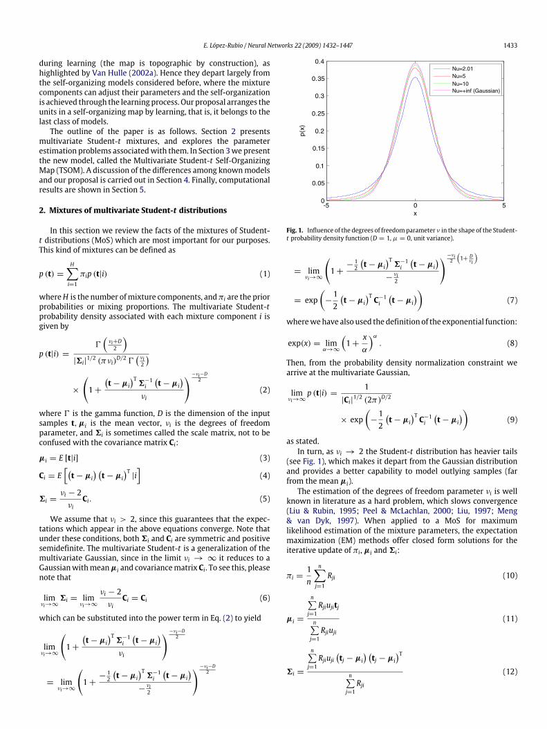
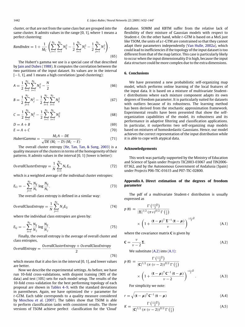
Fig. 1. Influence of the degrees of freedomparameter ν in the shape of the Student-t probability density function (D = 1, µ = 0, unit variance).

= limνi→∞

(1+−12

(t− µi

)T6−1i

(t− µi

)−νi2

)−νi2

(1+ Dνi

)

= exp(−12

(t− µi

)T C−1i (t− µi

))(7)

wherewehave also used thedefinition of the exponential function:

exp(x) = limα→∞

(1+

xα

)α. (8)

Then, from the probability density normalization constraint wearrive at the multivariate Gaussian,

limνi→∞

p (t|i) =1

|Ci|1/2 (2π)D/2

× exp(−12

(t− µi

)T C−1i (t− µi

))(9)

as stated.In turn, as νi → 2 the Student-t distribution has heavier tails

(see Fig. 1), which makes it depart from the Gaussian distributionand provides a better capability to model outlying samples (farfrom the mean µi).The estimation of the degrees of freedom parameter νi is well

known in literature as a hard problem, which slows convergence(Liu & Rubin, 1995; Peel & McLachlan, 2000; Liu, 1997; Meng& van Dyk, 1997). When applied to a MoS for maximumlikelihood estimation of the mixture parameters, the expectationmaximization (EM) methods offer closed form solutions for theiterative update of πi, µi and 6i:

πi =1n

n∑j=1

Rji (10)

µi =

n∑j=1Rjiujitj

n∑j=1Rjiuji

(11)

6i =

n∑j=1Rjiuji

(tj − µi

) (tj − µi

)Tn∑j=1Rji

(12)

1434 E. López-Rubio / Neural Networks 22 (2009) 1432–1447

where n is the number of input samples, Rji is the posteriorprobability that mixture component i generated the sample tj,

Rji = P(i|tj)

(13)

and uji is an auxiliary parameter:

uji =νi + D

νi +(tj − µi

)T6−1i

(tj − µi

) . (14)

However, there is no closed form solution for updating νi, and anonlinear equation in νi must be solved. For Peel and McLachlan’s(2000) and Shoham’s (2002) methods, these nonlinear equationsread

Peel: − ψ(νi2

)+ log

(νi2

)+ 1+

n∑j=1Rji(log uji − uji

)n∑j=1Rji

+ψ

(νi + D2

)− log

(νi + D2

)= 0 (15)

Shoham: log(νi2

)+ 1− ψ

(νi2

)+

n∑j=1Rji(lji − uji

)n∑j=1Rji

= 0 (16)

where ψ is the digamma (psi) function, and lji is another auxiliaryparameter which is computed as

lji = ψ(νi + D2

)+ log

2

νi +(tj − µi

)T6−1i

(tj − µi

) . (17)

The reader is kindly invited to see both papers for a moredetailed discussion. In our proposal, we consider both methods asoptions to estimate νi. They are iterative methods which rely ona startup value for νi, since the update equations for νi dependon 6i through the per-sample values uji and lji, and in turn theestimation of 6i depends on νi. As a third option, a non-iterativemethod is detailed in Appendix A, i.e. a direct method whichestimates νi without the need of a previous estimation of νi. Thisreduces the undesirable effects of poor initial estimations of νi andinterchanges of errors between νi and6i. Fromnowon, these threeoptions will be called ‘Peel’, ‘Shoham’ and ‘Direct’, respectively.

3. Multivariate Student-t Self-Organizing Map (TSOM)

3.1. Model definition

The TSOM model is defined as a mixture of H multivariateStudent-t components, just as presented in the previous section,Eqs. (1) and (2).At each time step n the network is presented a data sample tn.

We introduce a discrete hidden variable zn whose value (from 1 toH) indicates which component generated the data sample tn:

∀n∀i ∈ {1, . . . ,H} , P (zn = i) = πi (18)∀n∀i ∈ {1, . . . ,H} , p (tn|zn = i) = p(tn|i). (19)

In order to achieve self-organization, we only allow distributionmodels for zn which have the property that one component is themost probable and the probability decreases with the topologicaldistance to that component (see Luttrell (1990), Verbeek et al.(2005)). A topology is defined in the network so that the topologicaldistance betweenmixture components i and j is called δ(i, j). A flat,evenly spaced rectangular lattice of size rows× colsmay be used:

δ (i, j) =∥∥(ix, iy)− (jx, jy)∥∥ (20)

where (ix, iy) is the coordinate vector of mixture component i inthe lattice, and ix ∈ {1, . . . , cols}, iy ∈ {1, . . . , rows}. This is aimedto map the D-dimensional input space into the two-dimensionallattice space. Other lattice topologies and/or geometries could alsobe considered, like hexagonal lattice topologies and toroidal latticegeometries, depending on the structure of the input dataset andthe needs of the application at hand (Merenyi & Tasdemir, 2009).Hence we consider the following set of distributions Qn =

{qn1, . . . , qnH} for zn:

∀i, j ∈ {1, . . . ,H} ,

qnj (zn = i) = Pnj (zn = i) = P(zn = i|qnj

)∝ exp

(−δ (i, j)1 (n)

),(21)

where∑Hi=1 qnj (zn = i) = 1. Here the probability qnj (zn = i) is

analogous to Heskes’ confusion probability that the input sampletn has been generated by mixture component i instead of mixturecomponent j (Heskes, 2001; Van Hulle, 2005):

∀i, j ∈ {1, . . . ,H} ,qnj (zn = i) = P (unit i generated tn|tn is assigned to unit j) .

(22)

Verbeek et al. (2005) have also worked in this line. Eachdistribution qnj is ‘centered’ around unit j, that is, the probabilityqnj (zn = j) that j actually generated tn is the highest, while itsneighbors in the lattice get lower probabilities qnj (zn = i) as i isfarther from j. Note that δ is the topological distance function and1(n) is the neighborhood width, which is a positive decreasingfunction of n such that1(n)→ 0 as n→∞. A standard choice isthe linear decay:

1 (n) = 1 (0)(1−

nN

)(23)

where N is the total number of time steps. In the experiments wehave used an initial value1(0) = (rows+ cols)/2 for rows× colstopologies. This ensures that the neighborhoods are large at thebeginning, when the map needs to be plastic.For brevity we note

qnji = qnj (zn = i) = Pnj (zn = i) = P(zn = i|qnj

). (24)

For each time step n and distribution qnj we have

p(tn|qnj

)=

H∑i=1

qnjip (tn|i) . (25)

Then, a maximum likelihood approach is used to decide whichdistribution from Qn has the most probability p(qnj|tn) of havinggenerated the sample tn. This distribution is called the winningdistribution. The prior probabilities P(qnj) are assumed equal,i.e., P(qnj) = 1/H ∀j and so we have:

Winner (n) = argmaxj

{p(qnj|tn

)}

= argmaxj

P(qnj)p(tn|qnj

)H∑k=1P (qnk) p (tn|qnk)

= argmax

j

{p(tn|qnj

)}. (26)

This selection of a distribution from the set of distributions Qnenforces the self-organization of the network. This is because everydistribution qnj in Qn gives a decreasing posterior probability tothe units as their topological distance to unit j increases, and theposterior probability is proportional to the rate of update, as wewill see in the next subsection. When the winning distribution qnh


has been selected, we may compute the posterior probability Rnithat mixture component i generated the observed sample tn, giventhe set of possible distributions Qn:

Rni = P(i|tn,Qn) = P(i|qnh) = qnhi, where h = Winner (n) . (27)

After this competition, the mixture components are updatedaccording to Rni and tn in order to build a self-organizing map.

3.2. Learning method

When a new sample tn has been presented to the network, itsinformation should be used to update the mixture components.If we want to update mixture components i with the informationfrom sample tn, an online learning method for a MoS is required.This strategy has been examined by Sato and Ishii (2000) forgeneral (non-self-organizing) Gaussian PCA mixtures. Our onlinemethod generates the updated values πi(n), µi(n), νi(n) and Ci(n)for each mixture component i from the old values πi(n − 1),µi(n−1), νi(n−1), Ci(n−1), the new sample tn and the posteriorprobability Rni. The application of the Robbins–Monro stochasticapproximation algorithm yields the following update equations(see Appendix B for details):

πi (n) = (1− ε (n)) πi (n− 1)+ ε (n) Rni (28)mi (n) = (1− ε (n))mi (n− 1)+ ε (n) Rnitn (29)

µi (n) =mi (n)πi (n)

(30)

Mi (n) = (1− ε (n))Mi (n− 1)+ ε (n) Rni (tn − µi (n))× (tn − µi (n))

T (31)

Ci (n) =Mi (n)πi (n)

(32)

Peel: ωi (n) = (1− ε (n)) ωi (n− 1)+ ε (n) Rni

×

(log

(νi (n− 1)+ D

νi (n− 1)+ (tn − µi (n))T 6−1i (n− 1) (tn − µi (n))

)

−νi (n− 1)+ D


)(33)

Shoham: ωi (n) = (1− ε (n)) ωi (n− 1)+ ε (n) Rni

×

(log

(2

νi (n− 1)+ (tn − µi (n))TΣ−1i (n− 1) (tn − µi (n))

)

−νi (n− 1)+ D


)(34)

Direct: ωi (n) = (1− ε (n)) ωi (n− 1)

+ ε (n) Rni log√(t− µi (n))

T C−1i (n) (t− µi (n)) (35)

γi (n) =ωi (n)πi (n)

. (36)

Wemust remark thatmi(n),Mi(n),ωi(n) and γi(n) are auxiliaryvariables required to update themodel parametersπi,µi andCi. Onthe other hand, Eqs. (33) and (34) use the old values νi(n− 1) and6i(n − 1) because the new ones are not available yet. Please notethat the influence of the new sample tn in the new parameters isstronger as the posterior probability Rni is higher. In turn, since Rnidepends on the network topology (as seen in the previous subsec-tion), the rate of update depends on the topological distance,whichleads to self-organization. That is, Rni plays a role similar to that ofthe neighborhood function in the original SOM (Kohonen, 1990).In addition to those update equations, νi(n)must be computed

by solving one of these nonlinear equations, depending on the

selected option:

Peel : −ψ(νi (n)2

)+ log

(νi (n)2

)+ 1+ γi (n)

+ψ

(νi (n)+ D2

)− log

(νi (n)+ D2

)= 0 (37)

Shoham : log(νi (n)2

)+ 1− ψ

(νi (n)2

)+ γi (n) = 0 (38)

Direct : γi (n)−12

(ψ

(D2

)− ψ

(νi (n)2

)− log

(1

νi (n)− 2

))= 0. (39)

Please note that νi(n) is the only unknown in the three previousequations. These three options for obtaining νi(n) have beendescribed in Section 2 and Appendix A. For the ‘Direct’ option(Appendix A), νi(n − 1) is not used to compute the updatedparameter ωi(n). As we have mentioned earlier, this ensures thatthe possible estimation errors in νi(n−1) are not carried forward toνi(n). The problem of carrying the estimation errors fromπi(n−1),µi(n− 1) and Ci(n− 1) to πi(n), µi(n) and Ci(n) remains, but it isless important, since the stochastic approximationmethod ensuresthat the estimation errors for πi, µi and Ci are averaged out asn→∞ (see Appendix B).We obtain 6i(n) from Ci(n) and νi(n):

6i (n) =νi (n)− 2νi (n)

Ci (n) . (40)

Finally, ε(n) is the step size of the Robbins–Monro algorithmand is typically chosen as

ε (n) =1

an+ b, 0 < a < 1. (41)

In our experiments we have found that selecting b = 1a

often yields good results because the network remains plastic longenough. So, we have used in practice

ε (n) =1

ε0n+ 1ε0

, 0 < ε0 < 1 (42)

where ε0 is near to zero because higher values produce anexcessive plasticity (variability) of the estimations.

3.3. Map initialization

The initialization of each mixture component is achieved byestimating its starting parameters from a randomly chosen set ofsamples, which is different for each mixture component. For eachmixture component iwe select K samples tn, andwe compute theirmean as µi(0):

µi (0) =1K

K∑n=1

tn. (43)

The value of K is not crucial, provided that it is higher than Din order to avoid degenerate covariance matrices. We have usedK = 10D in the experiments. Then we compute their differenceswith µi(0) to yield Ci(0):

Ci (0) =1K

K∑n=1

(tn − µi (0)

) (tn − µi (0)

)T. (44)


The initial mixing probabilities are assumed to be equal:

πi (0) =1H. (45)

The following auxiliary variables are estimated following theirdefinitions (B.20) and (B.21):

mi (0) =1HK

K∑n=1

tn =1Hµi (0) (46)

Mi (0) =1HK

K∑n=1

(tn − µi (0)

) (tn − µi (0)

)T=1HCi (0) . (47)

There are two mechanisms to obtain νi(0). If we have selected‘Peel’ or ‘Shoham’ options, we need to choose νi(0) independentlyfrom the data, since these two methods do not allow to obtain anestimation of νi if we do not have a previous estimation. We haveused νi(0) = 103, which makes the mixture component nearlyGaussian. Then we obtain γi(0) by approximating (B.1) and (B.2):

Peel : ωi (0) =1HK

K∑n=1

×

[log

(νi (0)+ D

νi (0)+(tn − µi (0)

)TΣi (0)−1

(tn − µi (0)

))

−νi (0)+ D

νi (0)+(tn − µi (0)

)T6i (0)−1

(tn − µi (0)

)] (48)

Shoham : ωi (0) =1HK

K∑n=1

×

[log

(2

νi (0)+(tn − µi (0)

)T6i (0)−1

(tn − µi (0)

))

−νi (0)+ D

νi (0)+(tn − µi (0)

)T6i (0)−1

(tn − µi (0)

)] . (49)

On the other hand, if we have selected the ‘Direct’ option, νi(0)can be estimated from the data by solving the following nonlinearequation in νi(0):

Hωi (0) =12

(ψ

(D2

)− ψ

(νi (0)2

)− log

(1

νi (0)− 2

))(50)

which is deduced from (A.13) and (B.22), and where

ωi (0) =1HK

K∑n=1

log√(

tn − µi (0))T C−1i (0)

(tn − µi (0)

). (51)

Finally, the procedure to obtain 6i(0) does not depend on thechosen option:

6i (0) =νi (0)− 2νi (0)

Ci (0) . (52)

3.4. Summary

The TSOMmodel can be summarized as follows:

1. Set the initial values πi(0), µi(0), Ci(0), mi(0), Mi(0), 6i(0),ωi(0) and νi(0) for all mixture components i, as explained inSection 3.3.

2. Choose an input sample tn and compute the winning distribu-tion by Eq. (18). Use (19) to compute the posterior responsibil-ities Rni.

3. For every component i, estimate its parameters πi(n), µi(n),Ci(n), mi(n) and Mi(n), by Eqs. (20)–(24). Then estimate theparameter ωi(n) by one of the Eqs. (25)–(27), depending on theoption. Finally, estimate the parameter γi(n) by (28).

4. For every component i, estimate its degrees of freedomparameter νi(n) by solving one of the nonlinear equations (29)–(31), depending on the option. Then use (32) to obtain 6i(n).

5. If themap has converged or themaximum time stepN has beenreached, stop. Otherwise, go to step 2.

4. Discussion

There are some self-organizing models in the literature withthe capability of learning probabilistic mixtures. Nowwe comparethem to the TSOMmodel.

(a) The Generative Topographic Mapping (GTM) by Bishop et al.(1998) is a constrained mixture of Gaussians where the modelparameters are determined by an EM algorithm. The t-GTMmodel extends Gaussian GTM to mixtures of multivariateStudent-t distributions (Vellido, 2006). Both GTM and t-GTMuse a single global transformation from the input space toa latent space where all the local models lie, while TSOMbuilds a local representation of the input space in eachmixturecomponent. In other words, the mixture components of GTMand t-GTM are fixed in the latent space (Van Hulle, 2002a), andonly the global transformation is learned. On the other hand,TSOMmixture components are able to change adaptively theirrelative positions in the input space. Therefore the emergenceof a meaningful computational map is a consequence ofthe self-organization of the mixture components. This is notthe case of GTM and t-GTM, where the components arearranged in a computational map at design time, without anylearning process. Furthermore, TSOM allows a topology withany dimensionality, and even closed topologies (ring, toroidal,etc.), while the topology of GTM and t-GTM is required to havethe same dimensionality as the latent space. Hence GTM andt-GTM are expected to be preferred if the task at hand needs aunique latent space, whereas TSOM offers more flexibility.

(b) The Self-Organizing Mixture Model (SOMM) by Verbeek et al.(2005) uses a modified version of the EM algorithm toachieve self-organization of Gaussian models with isotropiccovariance matrices. The drawbacks of the SOMM are thatit only works in batch mode, it is only developed forisotropic covariance matrices, and it has a relatively heavycomputational complexity with respect to the number ofneurons: O(H2) for SOMM versus TSOM’s O(H). There is aO(H) speedup of SOMM, but then it nearly reduces to aclassical batch SOM with an isotropic covariance matrix. Inthis setup, SOMM can be seen as an improvement over SOMwhich features a parsimonious probabilistic model, since itdoes not store the covariance matrices. TSOM features a betterrepresentation capability by learning full covariance matricesin O(d3), while SOMM could be more useful in applicationswhere this capability is not needed, since it runs in O(d).

(c) The kernel topographic maps by Van Hulle (2002a, 2002b,2005) define mixtures of Gaussian probability distributions,but they are rather constrained because only diagonal covari-ancematrices are considered. This is a problem if the local prin-cipal directions of the data are not alignedwith the input spacecoordinates, and the situation is worse as the input space di-mension grows. On the other hand, TSOM does not have thoseconstraints, so its capability to represent complex input distri-butions is higher.

(d) The Self-Organizing Mixture Networks model (Yin & Allinson,2001) learns the mean vector and the full covariance matrix


at each neuron. Hence, they are more flexible for therepresentation of complex input data than some of theprevious models, which only consider diagonal covariancematrices (SOMM, topographic maps). Nevertheless, the SOMNprobability model is a mixture of Gaussians, so it is a limit caseof the MoS probability model of TSOM.

Finally, it must be noted that TSOM is expected to be morerobust against outliers than the self-organizingmapsmentioned in(b), (c) and (d), because it is based in a MoS rather than a mixtureof Gaussians.

5. Experimental results

5.1. Self-organization experiments

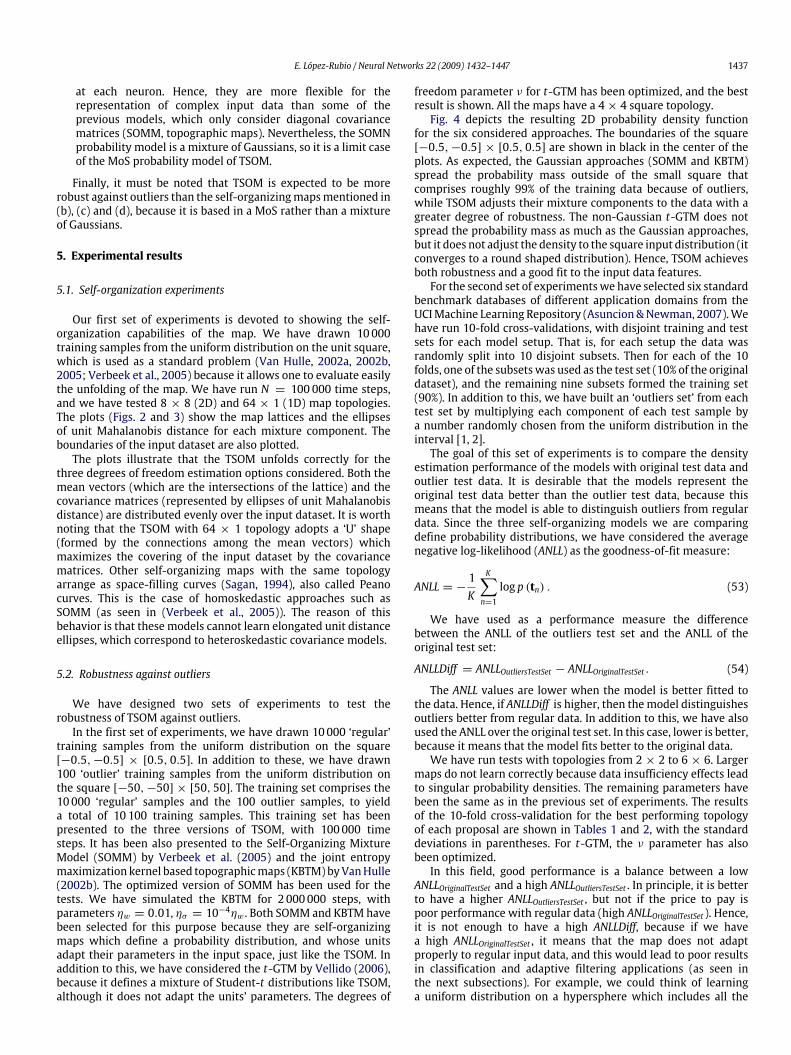
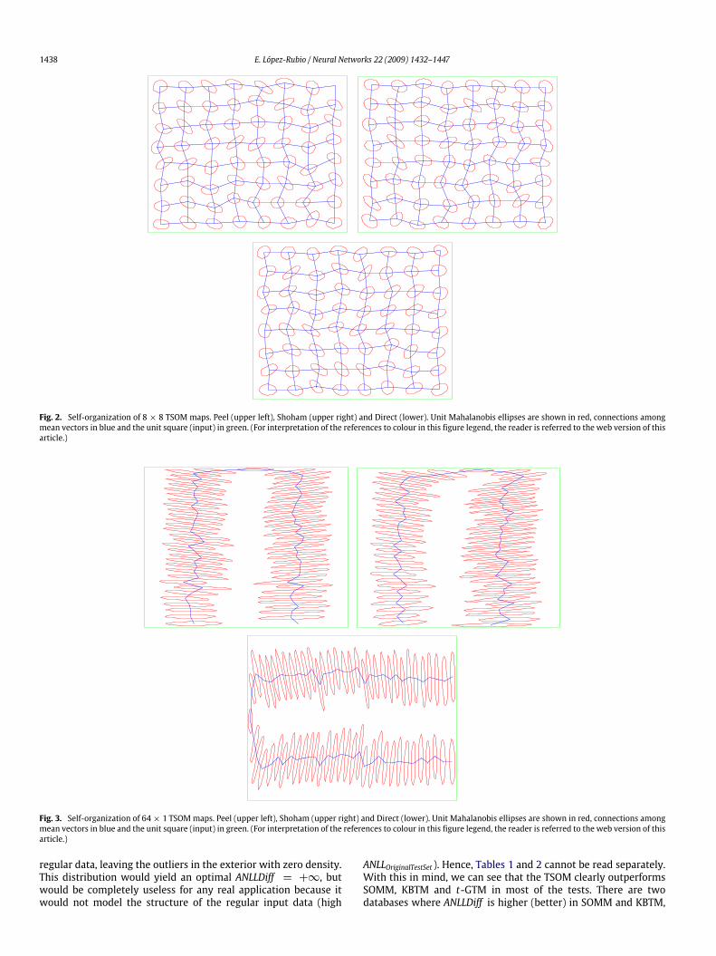
Our first set of experiments is devoted to showing the self-organization capabilities of the map. We have drawn 10000training samples from the uniform distribution on the unit square,which is used as a standard problem (Van Hulle, 2002a, 2002b,2005; Verbeek et al., 2005) because it allows one to evaluate easilythe unfolding of the map. We have run N = 100 000 time steps,and we have tested 8 × 8 (2D) and 64 × 1 (1D) map topologies.The plots (Figs. 2 and 3) show the map lattices and the ellipsesof unit Mahalanobis distance for each mixture component. Theboundaries of the input dataset are also plotted.The plots illustrate that the TSOM unfolds correctly for the

three degrees of freedom estimation options considered. Both themean vectors (which are the intersections of the lattice) and thecovariance matrices (represented by ellipses of unit Mahalanobisdistance) are distributed evenly over the input dataset. It is worthnoting that the TSOM with 64 × 1 topology adopts a ‘U’ shape(formed by the connections among the mean vectors) whichmaximizes the covering of the input dataset by the covariancematrices. Other self-organizing maps with the same topologyarrange as space-filling curves (Sagan, 1994), also called Peanocurves. This is the case of homoskedastic approaches such asSOMM (as seen in (Verbeek et al., 2005)). The reason of thisbehavior is that these models cannot learn elongated unit distanceellipses, which correspond to heteroskedastic covariance models.

5.2. Robustness against outliers

We have designed two sets of experiments to test therobustness of TSOM against outliers.In the first set of experiments, we have drawn 10000 ‘regular’

training samples from the uniform distribution on the square[−0.5,−0.5] × [0.5, 0.5]. In addition to these, we have drawn100 ‘outlier’ training samples from the uniform distribution onthe square [−50,−50] × [50, 50]. The training set comprises the10000 ‘regular’ samples and the 100 outlier samples, to yielda total of 10100 training samples. This training set has beenpresented to the three versions of TSOM, with 100000 timesteps. It has been also presented to the Self-Organizing MixtureModel (SOMM) by Verbeek et al. (2005) and the joint entropymaximization kernel based topographicmaps (KBTM) byVanHulle(2002b). The optimized version of SOMM has been used for thetests. We have simulated the KBTM for 2 000000 steps, withparameters ηw = 0.01, ησ = 10−4ηw . Both SOMM and KBTM havebeen selected for this purpose because they are self-organizingmaps which define a probability distribution, and whose unitsadapt their parameters in the input space, just like the TSOM. Inaddition to this, we have considered the t-GTM by Vellido (2006),because it defines a mixture of Student-t distributions like TSOM,although it does not adapt the units’ parameters. The degrees of

freedom parameter ν for t-GTM has been optimized, and the bestresult is shown. All the maps have a 4× 4 square topology.Fig. 4 depicts the resulting 2D probability density function

for the six considered approaches. The boundaries of the square[−0.5,−0.5] × [0.5, 0.5] are shown in black in the center of theplots. As expected, the Gaussian approaches (SOMM and KBTM)spread the probability mass outside of the small square thatcomprises roughly 99% of the training data because of outliers,while TSOM adjusts their mixture components to the data with agreater degree of robustness. The non-Gaussian t-GTM does notspread the probability mass as much as the Gaussian approaches,but it does not adjust the density to the square input distribution (itconverges to a round shaped distribution). Hence, TSOM achievesboth robustness and a good fit to the input data features.For the second set of experimentswe have selected six standard

benchmark databases of different application domains from theUCIMachine Learning Repository (Asuncion &Newman, 2007).Wehave run 10-fold cross-validations, with disjoint training and testsets for each model setup. That is, for each setup the data wasrandomly split into 10 disjoint subsets. Then for each of the 10folds, one of the subsetswas used as the test set (10% of the originaldataset), and the remaining nine subsets formed the training set(90%). In addition to this, we have built an ‘outliers set’ from eachtest set by multiplying each component of each test sample bya number randomly chosen from the uniform distribution in theinterval [1, 2].The goal of this set of experiments is to compare the density

estimation performance of the models with original test data andoutlier test data. It is desirable that the models represent theoriginal test data better than the outlier test data, because thismeans that the model is able to distinguish outliers from regulardata. Since the three self-organizing models we are comparingdefine probability distributions, we have considered the averagenegative log-likelihood (ANLL) as the goodness-of-fit measure:

ANLL = −1K

K∑n=1

log p (tn) . (53)

We have used as a performance measure the differencebetween the ANLL of the outliers test set and the ANLL of theoriginal test set:

ANLLDiff = ANLLOutliersTestSet − ANLLOriginalTestSet . (54)

The ANLL values are lower when the model is better fitted tothe data. Hence, if ANLLDiff is higher, then themodel distinguishesoutliers better from regular data. In addition to this, we have alsoused the ANLL over the original test set. In this case, lower is better,because it means that the model fits better to the original data.We have run tests with topologies from 2 × 2 to 6 × 6. Larger

maps do not learn correctly because data insufficiency effects leadto singular probability densities. The remaining parameters havebeen the same as in the previous set of experiments. The resultsof the 10-fold cross-validation for the best performing topologyof each proposal are shown in Tables 1 and 2, with the standarddeviations in parentheses. For t-GTM, the ν parameter has alsobeen optimized.In this field, good performance is a balance between a low

ANLLOriginalTestSet and a high ANLLOutliersTestSet . In principle, it is betterto have a higher ANLLOutliersTestSet , but not if the price to pay ispoor performance with regular data (high ANLLOriginalTestSet ). Hence,it is not enough to have a high ANLLDiff, because if we havea high ANLLOriginalTestSet , it means that the map does not adaptproperly to regular input data, and this would lead to poor resultsin classification and adaptive filtering applications (as seen inthe next subsections). For example, we could think of learninga uniform distribution on a hypersphere which includes all the


Fig. 2. Self-organization of 8 × 8 TSOM maps. Peel (upper left), Shoham (upper right) and Direct (lower). Unit Mahalanobis ellipses are shown in red, connections amongmean vectors in blue and the unit square (input) in green. (For interpretation of the references to colour in this figure legend, the reader is referred to the web version of thisarticle.)

Fig. 3. Self-organization of 64× 1 TSOMmaps. Peel (upper left), Shoham (upper right) and Direct (lower). Unit Mahalanobis ellipses are shown in red, connections amongmean vectors in blue and the unit square (input) in green. (For interpretation of the references to colour in this figure legend, the reader is referred to the web version of thisarticle.)

regular data, leaving the outliers in the exterior with zero density.This distribution would yield an optimal ANLLDiff = +∞, butwould be completely useless for any real application because itwould not model the structure of the regular input data (high

ANLLOriginalTestSet ). Hence, Tables 1 and 2 cannot be read separately.With this in mind, we can see that the TSOM clearly outperformsSOMM, KBTM and t-GTM in most of the tests. There are twodatabases where ANLLDiff is higher (better) in SOMM and KBTM,


Fig. 4. Resulting pdfs with the 2D outliers dataset. From left to right and from top to bottom: TSOM-Peel, TSOM-Shoham, TSOM-Direct, SOMM, KBTM and t-GTM (ν = 5).The color scale of log-densities is shown below.

Table 1Values of ANLLDiff (higher is better). Standard deviations in parentheses.

TSOM-Peel TSOM-Shoham TSOM-Direct SOMM KBTM t-GTM

BalanceScale 97.3691 (11.9612) 120.291 (114.152) 54.7659 (6.3051) 14.8541 (1.2292) 6.6504 (0.8051) 2.3652 (0.2642)Cloud 50.9259 (3.9596) 49.0616 (1.5859) 98.3497 (9.6691) 36.3010 (7.1518) 8.8195 (1.8531) 6.7659 (2.7171)Dermatology 25.2812 (5.7496) 25.4477 (5.9062) 25.0782 (4.1827) 31.5952 (14.1781) 54.4775 (16.6401) 21.3622 (8.6808)Liver 23.8389 (6.9377) 29.7428 (7.7232) 51.1108 (13.7780) 40.0577 (14.0666) 10.7229 (5.5866) 4.2451 (1.5597)Vowel 188.687 (70.113) 87.7331 (19.3980) 398.760 (86.045) 62.2923 (4.7094) 14.9906 (1.0597) 5.1422 (0.7231)Wine 36.8415 (3.1096) 37.1887 (3.9362) 26.1385 (1.1509) 92.7497 (44.8702) 31.7422 (14.7973) 6.3333 (3.6135)

Table 2Values of ANLLOriginalTestSet (lower is better). Standard deviations in parentheses.


BalanceScale −9.8701 (3.1013) −11.5231 (3.4012) −13.0966 (2.5930) 6.4242 (0.1676) 6.7960 (0.0840) 5.7313 (0.3343)Cloud 18.1976 (0.1749) 17.9537 (0.6383) 18.6853 (0.7806) 44.7708 (0.9584) 57.1072 (0.7060) 23.1590 (1.5937)Dermatology 20.1348 (4.9360) 18.3548 (5.3606) 19.2716 (3.8712) 40.2724 (6.7493) 76.2212 (3.1162) 66.3444 (4.2168)Liver 22.9131 (1.7682) 22.3005 (1.1997) 24.3421 (4.1616) 23.9770 (2.0503) 26.3002 (1.4518) 39.8007 (2.9879)Vowel 10.0598 (2.3041) 6.7567 (1.3757) 11.0810 (1.3712) 1.9280 (0.2481) 8.7228 (0.2575) 14.6668 (0.9985)Wine 19.7171 (1.2261) 20.6540 (1.6405) 19.9207 (1.1140) 55.6953 (3.5391) 67.2223 (2.4507) 31.5301 (3.9079)


but ANLLOriginalTestSet is much higher (much worse) for these twomodels.

5.3. Adaptive filtering

In this subsection we present an application of the TSOM tononlinear adaptive filtering. The adaptive filter recovers at thereceiver the information transmitted through a communicationchannel subject to several imperfections such as interference,distortion and noise (Proakis, 2001). Barreto and Souza (2006)have provided a comprehensive evaluation of self-organizingmapsas tools for this task. They describe the Local Linear Mapping(LLM) architecture (Walter, Ritter, & Schulten, 1990; Martinetz,Berkovich, & Schulten, 1993), which allows a self-organizing mapto learn nonlinear input–output mappings. The input sample tn attime instant n is generated from a time window of size D whichslides over the input sequence χ(n):

tn = (χ (n) , χ (n− 1) , . . . , χ (n− D+ 1))T . (55)

Associated with each unit i of the map we have a coefficientvector ai ∈ RD. It comprises the coefficients of a Finite ImpulseResponse (FIR) filter:

ai (n) =(ai,0 (n) , . . . , ai,D−1 (n)

)T (56)

so that the output of the LLM, i.e. the predicted output sequencevalue, is obtained by processing the input sample with the filter ofthe winning unit:

κ (n) = aTWinner(n) (n) tn. (57)

The learning rule for the adaptive filters is obtained as follows(Barreto & Souza, 2006; Farhang-Boroujeny, 1998):

ai (n) = ai (n− 1)+α

‖tn‖2exp

(−δ (i,Winner (n))

1 (n)

)×(κ (n)− ai (n− 1)T tn

)tn (58)

where α is the adaptation step size, κ (n) is the true outputsequence value and the exponential is the neighborhood function.In principle, the above equation is valid for any self-organizingmap model. The value of α is usually kept small to facilitate theconvergence of the filter coefficients. We have used α = 10−4 inthe experiments.We have selected six well known time series prediction

benchmarks, namely CATS (Särkkä, Vehtari, & Lampinen, 2007),KOBE (Singh, Tampubolon, & Yadavalli, 2002), Santa Fe series Aand C (Tikka & Hollmén, 2008), Darwin (Manatsa, Chingombe,Matsikwa, & Matarira, 2008) and Mackey-Glass (Zhang, Chung, &Lo, 2008). These time series are freely available from Lendasse(2008), Hyndman (2008), Weigend and Gershenfeld (2008), West(2008), and Wan (2008), respectively. A natural performancemeasure is the Mean Squared Error of the output sequenceprediction:

MSE =1N

N∑n=1

(κ (n)− κ (n)

)2. (59)

Please note that since the benchmarks are time series predictionproblems, the desired output sequence value for time step n isthe value of the input sequence for time step n + 1, i.e. κ (n) =χ (n+ 1) ∀n. That is, our goal is to estimate the next value of thetime series given the D previous values.As before, we have run tests with topologies from 2×2 to 6×6.

The remaining parameters have been the same as in the previoussubsection. In this case we have not tested t-GTM, since it does notadapt the parameters of its units, so we cannot learn a filter in each

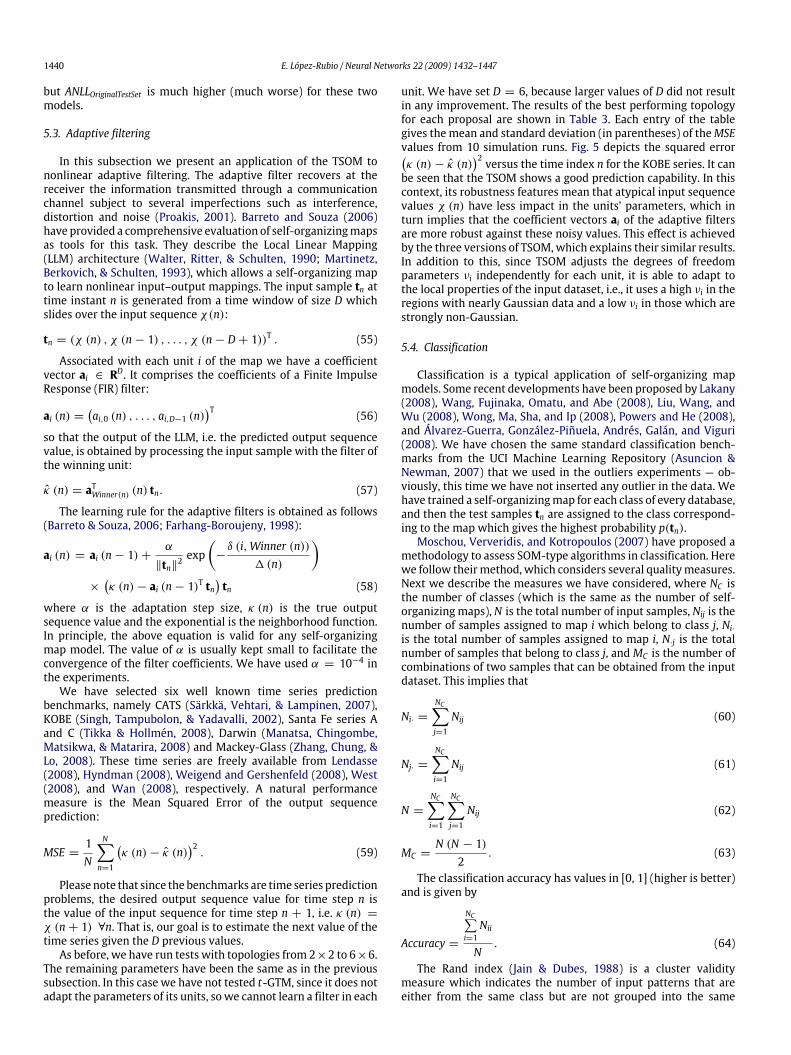
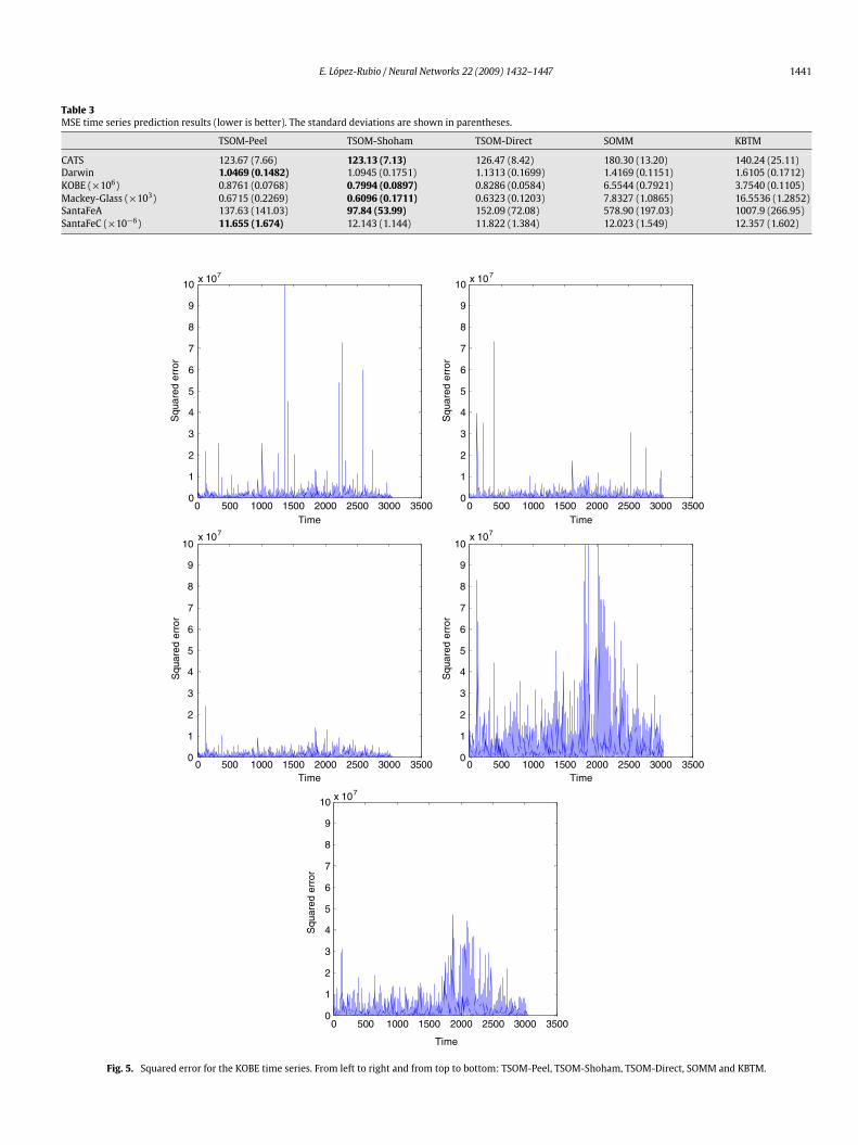
unit. We have set D = 6, because larger values of D did not resultin any improvement. The results of the best performing topologyfor each proposal are shown in Table 3. Each entry of the tablegives the mean and standard deviation (in parentheses) of theMSEvalues from 10 simulation runs. Fig. 5 depicts the squared error(κ (n)− κ (n)

)2 versus the time index n for the KOBE series. It canbe seen that the TSOM shows a good prediction capability. In thiscontext, its robustness features mean that atypical input sequencevalues χ (n) have less impact in the units’ parameters, which inturn implies that the coefficient vectors ai of the adaptive filtersare more robust against these noisy values. This effect is achievedby the three versions of TSOM, which explains their similar results.In addition to this, since TSOM adjusts the degrees of freedomparameters νi independently for each unit, it is able to adapt tothe local properties of the input dataset, i.e., it uses a high νi in theregions with nearly Gaussian data and a low νi in those which arestrongly non-Gaussian.

5.4. Classification

Classification is a typical application of self-organizing mapmodels. Some recent developments have been proposed by Lakany(2008), Wang, Fujinaka, Omatu, and Abe (2008), Liu, Wang, andWu (2008), Wong, Ma, Sha, and Ip (2008), Powers and He (2008),and Álvarez-Guerra, González-Piñuela, Andrés, Galán, and Viguri(2008). We have chosen the same standard classification bench-marks from the UCI Machine Learning Repository (Asuncion &Newman, 2007) that we used in the outliers experiments — ob-viously, this time we have not inserted any outlier in the data. Wehave trained a self-organizingmap for each class of every database,and then the test samples tn are assigned to the class correspond-ing to the map which gives the highest probability p(tn).Moschou, Ververidis, and Kotropoulos (2007) have proposed a

methodology to assess SOM-type algorithms in classification. Herewe follow theirmethod, which considers several qualitymeasures.Next we describe the measures we have considered, where NC isthe number of classes (which is the same as the number of self-organizing maps), N is the total number of input samples, Nij is thenumber of samples assigned to map i which belong to class j, Ni·is the total number of samples assigned to map i, N·j is the totalnumber of samples that belong to class j, andMC is the number ofcombinations of two samples that can be obtained from the inputdataset. This implies that

Ni· =NC∑j=1

Nij (60)

Nj· =NC∑i=1

Nij (61)

N =NC∑i=1

NC∑j=1

Nij (62)

MC =N (N − 1)

2. (63)

The classification accuracy has values in [0, 1] (higher is better)and is given by

Accuracy =

NC∑i=1Nii

N. (64)

The Rand index (Jain & Dubes, 1988) is a cluster validitymeasure which indicates the number of input patterns that areeither from the same class but are not grouped into the same


Table 3MSE time series prediction results (lower is better). The standard deviations are shown in parentheses.

TSOM-Peel TSOM-Shoham TSOM-Direct SOMM KBTM

CATS 123.67 (7.66) 123.13 (7.13) 126.47 (8.42) 180.30 (13.20) 140.24 (25.11)Darwin 1.0469 (0.1482) 1.0945 (0.1751) 1.1313 (0.1699) 1.4169 (0.1151) 1.6105 (0.1712)KOBE (×106) 0.8761 (0.0768) 0.7994 (0.0897) 0.8286 (0.0584) 6.5544 (0.7921) 3.7540 (0.1105)Mackey-Glass (×103) 0.6715 (0.2269) 0.6096 (0.1711) 0.6323 (0.1203) 7.8327 (1.0865) 16.5536 (1.2852)SantaFeA 137.63 (141.03) 97.84 (53.99) 152.09 (72.08) 578.90 (197.03) 1007.9 (266.95)SantaFeC (×10−6) 11.655 (1.674) 12.143 (1.144) 11.822 (1.384) 12.023 (1.549) 12.357 (1.602)

0 500 1000 1500 2000 2500 3000 35000

1

2

3

4

5

6

7

8

9

10 x 107

Time

Squ

ared

err

or

0 500 1000 1500 2000 2500 3000 35000

1

2

3

4

5

6

7

8

9

10 x 107

Time

Squ

ared

err

orS

quar

ed e

rror

Squ

ared

err

or

Squ

ared

err

or

0 500 1000 1500 2000 2500 3000 35000

1

2

3

4

5

6

7

8

9

10x 107

Time0 500 1000 1500 2000 2500 3000 3500

0

1

2

3

4

5

6

7

8

9

10x 107

Time

0 500 1000 1500 2000 2500 3000 35000

1

2

3

4

5

6

7

8

9

10 x 107

Time

Fig. 5. Squared error for the KOBE time series. From left to right and from top to bottom: TSOM-Peel, TSOM-Shoham, TSOM-Direct, SOMM and KBTM.


cluster, or that are not from the same class but are grouped into thesame cluster. It admits values in the range [0, 1], where 1 means aperfect clustering:

RandIndex = 1+1MC

(NC∑i=1

NC∑i=1

N2ij −12

NC∑i=1

N2i· −12

NC∑j=1

N2·j

).

(65)The Hubert’s gamma we use is a special case of that described

by Jain and Dubes (1988). It computes the correlation between thetwo partitions of the input dataset. Its values are in the interval[−1, 1], and 1 means a high correlation (good clustering):

A =12

NC∑i=1

NC∑i=1

N2ij −N2

(66)

B =12

NC∑j=1

N2·j −

12

NC∑i=1

NC∑i=1

N2ij (67)

C =12

NC∑i=1

N2i· −12

NC∑i=1

NC∑i=1

N2ij (68)

D = A+ B (69)E = A+ C (70)

HubertGamma =MCA− DE

√DE (MC − D) (MC − E)

. (71)

The overall cluster entropy (He, Tan, Tan, & Sung, 2003) is aqualitymeasure of the clusters in terms of the homogeneity of theirpatterns. It admits values in the interval [0, 1] (lower is better):

OverallClusterEntropy =1N

NC∑i=1

Ni·ECi (72)

which is a weighted average of the individual cluster entropies:

ECi = −NC∑j=1

NijNi·logNijNi·. (73)

The overall class entropy is defined in a similar way:

OverallClassEntropy =1N

NC∑j=1

N·jELj (74)

where the individual class entropies are given by:

ELj = −NC∑i=1

NijN·jlogNijN·j. (75)

Finally, the overall entropy is the average of overall cluster andclass entropies,

OverallEntropy =OverallClusterEntropy+ OverallClassEntropy

2(76)

whichmeans that it also lies in the interval [0, 1], and lower valuesare better.Nowwe describe the experimental settings. As before, we have

run 10-fold cross-validations, with disjoint training (90% of thedata) and test (10%) sets for each model setup. The results of the10-fold cross-validation for the best performing topology of eachproposal are shown in Tables 4–9, with the standard deviationsin parentheses. Again, we have optimized the ν parameter fort-GTM. Each table corresponds to a quality measure consideredby Moschou et al. (2007). The tables show that TSOM is ableto perform classification tasks with consistent results. The threeversions of TSOM achieve perfect classification for the ‘Cloud’

database. SOMM and KBTM suffer from the relative lack offlexibility of their mixture of Gaussian models with respect toStudent-t . On the other hand, while t-GTM is based on a MoS justlike TSOM, the units of a t-GTM are constrained so that they cannotadapt their parameters independently (Van Hulle, 2002a), whichcould lead to inefficiencies if the topology of the input dataset is toodifferent from that of themap lattice. This case is particularly likelyto occurwhen the input dimensionalityD is high, because the inputdata structure could bemore complex due to the extra dimensions.

6. Conclusions

We have presented a new probabilistic self-organizing mapmodel, which performs online learning of the local features ofthe input data. It is based on a mixture of multivariate Student-t distributions where each mixture component adapts its owndegrees of freedom parameter. It is particularly suited for datasetswith outliers because of its robustness. The learning methodhas been derived from the stochastic approximation framework.Experimental results have been presented that show the self-organization capabilities of the model, its robustness and itsperformance in adaptive filtering and classification applications.In particular, it outperforms two self-organizing map modelsbased on mixtures of homoskedastic Gaussians. Hence, our modelachieves the correct representation of the input distribution whileit is able to cope with atypical data.

Acknowledgements

This work was partially supported by the Ministry of Educationand Science of Spain under Projects TIC2003-03067 and TIN2006-07362, and by the Autonomous Government of Andalusia (Spain)under Projects P06-TIC-01615 and P07-TIC-02800.

Appendix A. Direct estimation of the degrees of freedomparameter

The pdf of a multivariate Student-t distribution is usuallyexpressed as

p (t) =0(ν+D2

)|6|1/2 (πν)D/2 0

(ν2

)×

(1+

(t− µ)T 6−1 (t− µ)ν

)−ν−D2

(A.1)

where the covariance matrix C is given by

C =ν

ν − 26. (A.2)

We substitute (A.2) into (A.1):

p (t) =0(ν+D2

)|C|1/2 (π (ν − 2))D/2 0

(ν2

)×

(1+

(t− µ)T C−1 (t− µ)ν − 2

)−ν−D2

. (A.3)

For simplicity we note:

r =√(t− µ)T C−1 (t− µ) (A.4)

K =0(ν+D2

)|C|1/2 (π (ν − 2))D/2 0

(ν2

) (A.5)


Table 4Classification accuracy (higher is better). Standard deviations in parentheses.



Table 5Rand index (higher is better). Standard deviations in parentheses.



Table 6Hubert’s gamma (higher is better). Standard deviations in parentheses.


BalanceScale 0.7511 (0.1149) 0.8188 (0.1003) 0.8013 (0.0796) 0.5004 (0.0930) 0.5058 (0.0721) 0.4344 (0.2422)Cloud 1.0000 (0.0000) 1.0000 (0.0000) 1.0000 (0.0000) 0.9983 (0.0054) 0.9798 (0.0165) 0.9691 (0.0306)Dermatology 0.9444 (0.0486) 0.9270 (0.0646) 0.9027 (0.0776) 0.7509 (0.1456) 0.1249 (0.1062) 0.3971 (0.2029)Liver 0.0870 (0.1138) 0.0645 (0.0715) 0.1116 (0.1161) 0.0050 (0.0457) −0.0054 (0.0277) 0.0202 (0.0575)Vowel 0.8241 (0.0607) 0.8153 (0.0712) 0.7901 (0.1099) 0.7799 (0.0390) 0.4018 (0.0571) 0.2699 (0.0509)Wine 0.8265 (0.1630) 0.8496 (0.1910) 0.9048 (0.1327) 0.4618 (0.1546) 0.5040 (0.2635) 0.4846 (0.2804)

Table 7Overall cluster entropy (lower is better). Standard deviations in parentheses.



Table 8Overall class entropy (lower is better). Standard deviations in parentheses.



Table 9Overall entropy (lower is better). Standard deviations in parentheses.



where r is the Mahalanobis distance. Now we evaluate Elog r:

E [log r] =∫(log r) p (t) dt

= K∫(log r)

(1+

r2

ν − 2

)−ν−D2

dt. (A.6)

The above integral is best computed if we change fromhyperelliptical coordinates to hyperspherical coordinates centeredinµ; seeMagdon-Ismail and Sill (2008) for an analogous derivationwith polar coordinates. The coordinate change is

y = A (t− µ) (A.7)

where A is the Cholesky decomposition matrix of C−1, and hencewe have


C−1 = ATA. (A.8)The integral now reads

E [log r] = |C|1/2 K∫(log r)

(1+

r2

ν − 2

)−ν−D2

dy (A.9)

where the Mahalanobis distance r is expressed as the standardEuclidean distance in the new coordinate system:

r =√yTy. (A.10)

A hyperspherical volume element of thickness dr has volume

dy =2πD/2

0(D2

) rD−1dr. (A.11)

Hence we get

E [log r] =2K |C|1/2 πD/2

0(D2

) ∫∞

0(log r) rD−1

×

(1+

r2

ν − 2

)−ν−D2

dr. (A.12)

After the evaluation of the integral and some simplifications,wearrive at

E [log r] =12

(ψ

(D2

)− ψ

(ν2

)− log

(1

ν − 2

)). (A.13)

The above equation expresses E log r as a strictly increasingfunction of ν. Hence it is straightforward to invert this functionalrelation numerically, so that we obtain a method to estimate νfrom an estimation of E log r . This has the advantage that we donot need any tentative value of ν to estimate E log r because rdepends on µ and C, but not on ν. This differs from Peel andMcLachlan (2000) and Shoham (2002), which propose iterativemethods to obtain successively finer approximations of ν, witheach iteration re-evaluating all the input samples to computethe next approximation. Our approach is better suited to onlinelearning, since the past input samples are not revisited.A similar reasoning can be used to compute Er2, and the result

is

E[r2]= D

ν − 2ν

. (A.14)

Despite the relative simplicity of this approach, we have notused it because it is more influenced by outliers than E log r .

Appendix B. Stochastic approximation

Let2i = (πi,µi, Ci, γi) be a vector comprising the parametersfor mixture component i, where γi is a parameter which is used toobtain the ‘degrees of freedom’ parameter νi, and depends on theselected method:

Peel : γi = E

[log

(νi + D

νi +(t− µi

)T6−1i

(t− µi

))

−νi + D

νi +(t− µi

)T6−1i

(t− µi

)] (B.1)

Shoham : γi = E

[log

(2

νi +(t− µi

)T6−1i

(t− µi

))

−νi + D

νi +(t− µi

)TΣ−1i

(t− µi

)] (B.2)

Direct : γi = E[log

√(t− µi

)T C−1i (t− µi

)]. (B.3)

Note that

6i =νi − 2νi

Ci. (B.4)

Let ϕ(2i, t) be an arbitrary function of2i and the input samplet. Then we define the weighted mean of ϕ(2i, t) as:

〈ϕ〉i = E [P (i|t) ϕ (Θi, t)] . (B.5)

This allows one to express the conditional expectation ofϕ(2i, t) as follows:

〈ϕ〉i

〈1〉i=E [P (i|t) ϕ (Θi, t)]

E [P (i|t)]=

∫p (t) P (i|t) ϕ (Θi, t) dt

πi

=

∫p (t) P (i|t)

πiϕ (Θi, t) dt =

∫p (t|i) ϕ (Θi, t) dt

= E [ϕ (Θi, t) |i] . (B.6)

Therefore we can rewrite the mixture parameters in terms ofthe weighted means 〈ϕ〉i:

πi = 〈1〉i (B.7)

µi =〈t〉i〈1〉i

(B.8)

Ci =

⟨(t− µi

) (t− µi

)T⟩i

〈1〉i(B.9)

Peel : γi =1〈1〉i

⟨log

(νi + D

νi +(t− µi

)T6−1i

(t− µi

))

−νi + D

νi +(t− µi

)T6−1i

(t− µi

)⟩i

(B.10)

Shoham : γi =1〈1〉i

⟨log

(2

νi +(t− µi

)T6−1i

(t− µi

))

−νi + D

νi +(t− µi

)T6−1i

(t− µi

)⟩i

(B.11)

Direct : γi =

⟨log

√(t− µi

)T C−1i (t− µi

)⟩i

〈1〉i. (B.12)

If we have n samples (finite case), the linear least squaresapproximation for 〈ϕ〉i is:

〈ϕ〉i =1n

n∑j=1

P(i|tj)ϕ(Θi, tj

)=1n

n∑j=1

Rjiϕ(Θi, tj

)(B.13)

where we should remember that the posterior probability thatmixture component i generated the sample tj is noted

Rji = P(i|tj). (B.14)

As n → ∞, the approximation of (B.13) converges to the exactvalue given by (B.5). Next we apply the Robbins–Monro stochasticapproximation algorithm (see Kushner and Yin (2003)) to estimateiteratively the value of the weighted means 〈ϕ〉i:

〈ϕ〉i (0) = P (i|t0) ϕ (Θi, t0) (B.15)

〈ϕ〉i (n) = 〈ϕ〉i (n− 1)+ ε (n) (P (i|tn) ϕ (Θi, tn)− 〈ϕ〉i (n− 1)) (B.16)

where ε(n) is the step size, which must satisfy the following con-ditions in order to guarantee convergence of the Robbins–Monro


method:

ε (n) > 0, limn→∞

ε (n) = 0,∞∑n=1

ε (n) = ∞,

∞∑n=1

ε2 (n) <∞.

(B.17)

In order to fulfill these requirements, ε(n) is typically selected as

ε (n) =1

an+ b, 0 < a < 1. (B.18)

On the other hand, Eq. (B.16) is more conveniently written as:

〈ϕ〉i (n) = (1− ε (n)) 〈ϕ〉i (n− 1)+ ε (n) Rniϕ (Θi, tn) . (B.19)

Now we derive an online stochastic approximation algorithm byapplying Eq. (B.19) to Eqs. (B.7)–(B.12). First we need to definethree auxiliary variables:

mi = 〈t〉i (B.20)

Mi =⟨(t− µi

) (t− µi

)T⟩i

(B.21)

ωi = 〈1〉i 〈γi〉i . (B.22)

Note that (B.22) compacts the three options in (B.10)–(B.12). Thecorresponding update equations are:

mi (n) = (1− ε (n))mi (n− 1)+ ε (n) Rnitn (B.23)

Mi (n) = (1− ε (n))Mi (n− 1)+ ε (n) Rni

(tn − µi (n)

) (tn − µi (n)

)T (B.24)Peel : ωi (n) = (1− ε (n)) ωi (n− 1)

+ ε (n) Rni

(log

(νi + D

νi +(tn − µi

)T6−1i

(tn − µi

))

−νi + D

νi +(tn − µi

)T6−1i

(tn − µi

)) (B.25)

Shoham : ωi (n) = (1− ε (n)) ωi (n− 1)+ ε (n) Rni

×

(log

(2

νi +(t− µi

)T6−1i

(t− µi

))

−νi + D

νi +(t− µi

)T6−1i

(t− µi

)) (B.26)

Direct : ωi (n) = (1− ε (n)) ωi (n− 1)

+ ε (n) Rni log√(

t− µi (n))T C−1i (n)

(t− µi (n)

)(B.27)

where the time step indexes for µi(n), 6i(n − 1) and νi(n − 1)have been dropped in the right-hand side of (B.25) and (B.26) forsimplicity. Note that we cannot use 6i(n) or νi(n) in (B.25) and(B.26) because they have not been computed yet. This is the effectof the self-dependence problem with ‘Peel’ and ‘Shoham’ methodsof estimating νi, which was discussed in Section 2.Then we are ready to rewrite (B.7)–(B.12):

πi (n) = (1− ε (n)) πi (n− 1)+ ε (n) Rni (B.28)

µi (n) =mi (n)πi (n)

(B.29)

Ci (n) =Mi (n)πi (n)

(B.30)

γi (n) =ωi (n)πi (n)

(B.31)

where again (B.31) compacts the three options in (B.10)–(B.12).Next, νi(n) is computed by either (15), (16) or (A.13), depending onthe chosen option. Finally, (B.4) is used to obtain 6i(n) from Ci(n)and νi(n).

Proposition. If (B.17) holds, then the stochastic approximationalgorithm of (B.23)–(B.31) converges to the exact solution of (B.7)–(B.12).

Proof. The general form of the Robbins–Monro stochastic algo-rithm is

θ (n+ 1) = θ (n)+ ε (n) Y (n) (B.32)

where, in our case we take

θ (n) =(〈ϕ〉i (n)

)ϕ,i . (B.33)

That is, we include all the weighted means in the currentestimation vector θ(n). We also take

Y (n) = ξ (n)− θ (n) (B.34)

where the new data to be incorporated into the estimation is

ξ (n) = (P (i|tn,Θ (n) ,Qn) ϕ (Θi (n) , tn))ϕ,i . (B.35)

In the above equation, 2 = (πi,µi, Ci, γi)i is the completeparameter vector of the self-organizing map, and Qn is thedistribution set which is used to enforce self-organization at timestep n. The goal of the stochastic algorithm is to find a root of theequation

g (θ (n)) = 0 (B.36)

where

g (θ (n)) =(E [P (i|t,Θ (n) ,Q∞) ϕ (Θi (n) , t)]

− 〈ϕ〉i (n))ϕ,i (B.37)

and Q∞ is the limit distribution set,

q∞ii = 1, q∞ij = 0 ∀i 6= j (B.38)

which is such that the Qn tend to Q∞ as n→∞:

limn→∞

qnij = q∞ij ∀i∀j. (B.39)

In order to prove the convergence of the algorithm, we aregoing to prove that the ‘‘noise’’ in the observation Yn is amartingaledifference (see (Kushner & Yin, 2003)). That is, there is a functiongn(·) of θ such that

E[Yn|θ (0) , Yj, j < n] = gn (θ (n)) . (B.40)

This is readily verified:

gn (θ (n)) = (E [P (i|t,Θ (n) ,Qn) ϕ (Θi (n) , t)])ϕ,i − θ (n) . (B.41)

Note that gn(θ(n)) only depends on n and θ(n), because Qn isobtained from n and2(n) can be computed from θ(n). So we havethat

Yn = gn (θ (n))+ δMn (B.42)

where δMn is amartingale difference. The associated ‘‘bias’’ processis defined as:

βn = E[Yn|θ (0) , Yj, j < n] − g (θ (n)) . (B.43)


We can guarantee convergence by proving the following threeconditions:

supnE[‖Yn‖2] <∞ (B.44)

limn→∞

βn = 0 (B.45)

∀m > 0 ∀θ, limn→∞

∥∥∥∥∥n+m∑j=n

εj(gj (θ)− g (θ)

)∥∥∥∥∥ = 0. (B.46)

Next we examine the first condition:

E[‖Yn‖2] = E[‖ξ (n)− θ (n)‖2]

=

∑ϕ,i

E[‖P (i|t,Θ (n) ,Qn) ϕ (Θi (n) , t)

− 〈ϕ〉i (n)‖2]. (B.47)

The above value is finite if we assume that the input distributionhas a compact support. This assumption should hold in practice,since real data always appear in a finite domain. Alternatively wecan relax this assumption by considering that the input densitydecreases exponentially as ‖t‖ → ∞.Now we study the second condition:

limn→∞

βn = limn→∞

(E[Yn|θ (0) , Yj, j < n] − g (θ (n))

)= limn→∞

(E [P (i|t,Θ (n) ,Qn) ϕ (Θi (n) , t)]

− E [P (i|t,Θ (n) ,Q∞) ϕ (Θi (n) , t)])ϕ,i . (B.48)

This limit is zero because (B.39) implies that

limn→∞

P (i|t,Θ (n) ,Qn) = P (i|t,Θ (n) ,Q∞) . (B.49)

Finally, for the third condition we have

∀θ, limj→∞

(gj (θ)− g (θ)

)= limj→∞

(E[P(i|t,Θ,Qj

)ϕ (Θi, t)]

− E [P (i|t,Θ,Q∞) ϕ (Θi, t)])ϕ,i (B.50)

which is also zero because of (B.39). In turn this means that thelimit

limn→∞

∥∥∥∥∥n+m∑j=n

εj(gj (θ)− g (θ)

)∥∥∥∥∥ (B.51)

is zero ∀m > 0∀θ since it is the norm of a finite sum of two factorswhere both tend to zero.Hence we have proved that the algorithm converges to a root of

Eq. (B.36). At convergence we have

〈ϕ〉i (n) = E [P (i|t,Θ (n) ,Q∞) ϕ (Θi (n) , t)] ∀ϕ∀i (B.52)

which is equivalent to the true value of the weighted mean, givenby (B.5). Therefore, (B.52) is the exact solution of (B.7)–(B.12). �

References

Álvarez-Guerra, M., González-Piñuela, C., Andrés, A., Galán, B., & Viguri, J. R.(2008). Assessment of self-organizing map artificial neural networks for theclassification of sediment quality. Environment International, 34(6), 782–790.

Asuncion, A., & Newman, D. J. (2007). UCI machine learning repository. Irvine, CA:University of California, Department of Information and Computer Science.http://www.ics.uci.edu/∼mlearn/MLRepository.html.

Barreto, G. A., & Souza, L. G. M. (2006). Adaptive filtering with the self-organizingmap: A performance comparison. Neural Networks, 19(6–7), 785–798.

Bickel, P. J., & Levina, E. (2007). Regularized estimation of large covariancematrices.Annals of Statistics, 36(1), 199–227.

Bishop, C. M., Svensen, M., & Williams, C. K. I. (1998). GTM: The generativetopographic mapping. Neural Computation, 10(1), 215–234.

Brugger, D., Bogdan, M., & Rosenstiel, W. (2008). Automatic cluster detection inKohonen’s SOM. IEEE Transactions on Neural Networks, 19(3), 442–459.

Chatzis, S., & Varvarigou, T. (2008). Robust fuzzy clustering using mixtures ofStudent’s-t distributions. Pattern Recognition Letters, 29(13), 1901–1905.

Chen, W.-C., Tai, P.-H., Wang, M.-W., Deng, W.-J., & Chen, C.-T. (2008). A neuralnetwork-based approach for dynamic quality prediction in a plastic injectionmolding process. Expert Systems with Applications, 35(3), 843–849.

Ciaramella, A., Cocozza, S., Iorio, F., Miele, G., Napolitano, F., Pinelli, M., Raiconi, G., &Tagliaferri, R. (2008). Interactive data analysis and clustering of genomic data.Neural Networks, 21(2–3), 368–378.

Correa, R. F., & Ludermir, T. B. (2008). A quickly trainable hybrid SOM-baseddocument organization system. Neurocomputing , 71(16–18), 3353–3359.

Dittenbach, M., Rauber, A., & Merkl, D. (2002). The growing hierarchicalself-organizing map: Exploratory analysis of high-dimensional data. IEEETransactions on Neural Networks, 13(6), 1331–1341.

Dokur, Z., & Ölmez, T. (2008). Heart sound classification using wavelet transformand incremental self-organizing map. Digital Signal Processing , 18(6), 951–959.

Farhang-Boroujeny, B. (1998). Adaptive filters, theory and applications. John Wiley &Sons.

Fukushima, K. (1999). Self-organization of shift-invariant receptive fields. NeuralNetworks, 12(6), 791–802.

He, J., Tan, A. H., Tan, C. L., & Sung, S. Y. (2003). On quantitative evaluation ofclustering systems. In W. Wu, H. Xiong, & S. Shekhar (Eds.), Clustering andinformation retrieval (pp. 105–133). Norwell, MA: Kluwer Academic Publishers.

Heskes, T. (2001). Self-organizingmaps, vector quantization, andmixturemodeling.IEEE Transactions on Neural Networks, 12(6), 1299–1305.

Hoffbeck, J., & Landgrebe, D. (1996). Covariancematrix estimation and classificationwith limited training data. IEEE Transactions on Pattern Analysis and MachineIntelligence, 18(7), 763–767.

Hyndman, R. J. (2008). Time series data library. Available at: http://www.robhyndman.info/TSDL.

Jain, A. K., & Dubes, R. C. (1988). Algorithms for clustering data. Englewood Cliffs, NJ:Prentice-Hall.

Kiang, M. Y., & Fisher, D. M. (2008). Selecting the right MBA schools — Anapplication of self-organizing map networks. Expert Systems with Applications,35(3), 946–955.

Kohonen, T. (1990). The self-organizingmap. Proceedings of the IEEE, 78, 1464–1480.Kosinski, A. (1999). A procedure for the detection of multivariate outliers.Computational Statistics and Data Analysis, 29(2), 145–161.

Kushner, H. J., & Yin, G. G. (2003). Stochastic approximation and recursive algorithmsand applications (2nd ed.). New York: Springer-Verlag.

Laaksonen, J., Koskela, M., & Oja, E. (2002). PicSOM-self-organizing image retrievalwith MPEG-7 content descriptors. IEEE Transactions on Neural Networks, 13(4),841–853.

Laaksonen, J., Koskela, M., & Oja, E. (2004). Class distributions on SOM surfaces forfeature extraction and object retrieval. Neural Networks, 17(8–9), 1121–1133.

Lakany, H. (2008). Extracting a diagnostic gait signature. Pattern Recognition, 41(5),1644–1654.

Lendasse, A. (2008). Time series prediction competition: The CATS benchmark.Available at: http://www.cis.hut.fi/lendasse/competition/competition.html.

Liu, C., & Rubin, D. B. (1995). ML estimation of the t distribution using EM and itsextensions, ECM and ECME. Statistica Sinica, 5, 19–39.

Liu, C. (1997).ML estimation of themultivariate t distribution and the EMalgorithm.Journal of Multivariate Analysis, 63(2), 296–312.

Liu, Y., Wang, X., & Wu, C. (2008). ConSOM: A conceptional self-organizing mapmodel for text clustering. Neurocomputing , 71(4–6), 857–862.

Luttrell, S. P. (1990). Derivation of a class of training algorithms. IEEE Transactionson Neural Networks, 1(2), 229–232.

Magdon-Ismail, M., & Sill, J. (2008). A linear fit gets the correct monotonicitydirections.Machine Learning , 70(1), 21–43.

Manatsa, D., Chingombe, W., Matsikwa, H., & Matarira, C. H. (2008). The superiorinfluence of Darwin sea level pressure anomalies over ENSO as a simple droughtpredictor for Southern Africa. Theoretical and Applied Climatology, 92(1–2), 1–14.

Martinetz, T. M., Berkovich, S. G., & Schulten, K. J. (1993). Neural-gas networkfor vector quantization and its application to time-series prediction. IEEETransactions on Neural Networks, 4(4), 558–569.

McLachlan, G. J., Bean, R. W., & Peel, D. (2002). A mixture model-based approach tothe clustering of microarray expression data. Bioinformatics, 18(3), 413–422.

Meng, X.-L., & van Dyk, D. (1997). The EM algorithm—An old folk-song sung to a fastnew tune. Journal of the Royal Statistical Society Series B, 59(3), 511–567.

Merenyi, E., & Tasdemir, K. (2009). Exploiting data topology in visualization andclustering of self-organizing maps. IEEE Transactions on Neural Networks, 20(4),549–562.

Moschou, V., Ververidis, D., & Kotropoulos, C. (2007). Assessment of self-organizingmap variants for clustering with application to redistribution of emotionalspeech patterns. Neurocomputing , 71(1–3), 147–156.

Peel, D., &McLachlan, G. J. (2000). Robustmixturemodelling using the t distribution.Statistics and Computing , 10(4), 339–348.

Powers, S. T., & He, J. (2008). A hybrid artificial immune system and self organisingmap for network intrusion detection. Information Sciences, 178(15), 3024–3042.

Prieto, B., Tricas, F., Merelo, J. J., Mora, A., & Prieto, A. (2008). Visualizing theevolution of a web-based social network. Journal of Network and ComputerApplications, 31(4), 677–698.

Proakis, J. G. (2001). Digital communications. New York: McGraw-Hill.Rocke, D. M., & Woodruff, D. L. (1997). Robust estimation of multivariate locationand shape. Journal of Statistical Planning and Inference, 57, 245–255.

Sagan, H. (1994). Space-filling curves. Springer-Verlag.

http://www.ics.uci.edu/~mlearn/MLRepository.html








http://www.robhyndman.info/TSDL





http://www.cis.hut.fi/lendasse/competition/competition.html










Särkkä, S., Vehtari, A., & Lampinen, J. (2007). CATS benchmark time series predictionby Kalman smoother with cross-validated noise density. Neurocomputing ,70(13–15), 2331–2341.

Sato, M., & Ishii, S. (2000). On-line EM algorithm for the normalized Gaussiannetwork. Neural Computation, 12(2), 407–432.

Shoham, S. (2002). Robust clustering by deterministic agglomeration EM ofmixtures of multivariate t-distributions. Pattern Recognition, 35(5), 1127–1142.

Singh, N., Tampubolon, D., & Yadavalli, V. S. S. (2002). Time series modelling oftheKobe–Osaka earthquake recordings. International Journal ofMathematics andMathematical Sciences, 29(8), 467–479.

Svensén, M., & Bishop, C. M. (2005). Robust Bayesian mixture modelling.Neurocomputing , 64, 235–252.

Tikka, J., & Hollmén, J. (2008). Sequential input selection algorithm for long-termprediction of time series. Neurocomputing , 71(13–15), 2604–2615.

Van Hulle, M.M. (2002a). Kernel-based topographicmap formation by local densitymodeling. Neural Computation, 14(7), 1561–1573.

Van Hulle, M. M. (2002b). Joint entropy maximization in Kernel-based topographicmaps. Neural Computation, 14(8), 1887–1906.

Van Hulle, M. M. (2005). Maximum likelihood topographic map formation. NeuralComputation, 17(3), 503–513.

Vellido, A. (2006). Missing data imputation through GTM as a mixture of t-distributions. Neural Networks, 19(10), 1624–1635.

Verbeek, J. J., Vlassis, N., & Krose, B. J. A. (2005). Self-organizing mixture models.Neurocomputing , 63, 99–123.

Walter, J., Ritter, H., & Schulten, K. (1990). Non-linear predictionwith self organizingmap. Proceedings of the IEEE International Joint Conference on Neural Networks, 1,587–592.

Wan, E. A. (2008). Time series data. http://www.cse.ogi.edu/∼ericwan/data.html.Wang, B., Fujinaka, T., Omatu, S., & Abe, T. (2008). Automatic inspection oftransmission devices using acoustic data. IEEE Transactions on AutomationScience and Engineering , 5(2), 361–367.

Weigend, A. S., & Gershenfeld, N. A. (2008). The Santa Fe time series competition data.http://www-psych.stanford.edu/∼andreas/Time-Series/SantaFe/.

West, M. (2008). Some time series data sets. Available at: http://www.isds.duke.edu/∼mw/ts_data_sets.html.

Wong, H.-S., Ma, B., Sha, Y., & Ip, H. H. S. (2008). 3D head model retrieval in kernelfeature space using HSOM. Pattern Recognition, 41(2), 468–483.

Yin, H., & Allinson, N. M. (2001). Self-organizing mixture networks for probabilitydensity estimation. IEEE Transactions on Neural Networks, 12(2), 405–411.

Zhang, J., Chung, H. S.-H., & Lo, W.-L. (2008). Chaotic time series predictionusing a neuro-fuzzy system with time-delay coordinates. IEEE Transactions onKnowledge and Data Engineering , 20(7), 956–964.

Zhao, J., & Jiang, Q. (2006). Probabilistic PCA for t distributions. Neurocomputing ,69(16–18), 2217–2226.

http://www.cse.ogi.edu/~ericwan/data.html








http://www-psych.stanford.edu/~andreas/Time-Series/SantaFe/







http://www.isds.duke.edu/~mw/ts_data_sets.html










multivariate student- self-organizing maps

Documents