multivariate topology simplificationmultivariate topology simplification amit chattopadhyay ∗...
TRANSCRIPT

arX
iv:1
509.
0446
5v1
[cs.
CG
] 15
Sep
201
5
Multivariate Topology Simplification
Amit Chattopadhyay∗ Hamish Carr† David Duke‡ Zhao Geng§ Osamu Saeki¶
October 2, 2018
Abstract
Topological simplification of scalar and vector fields is well-established as an effective method for analysing and visualisingcomplex data sets. For multi-field data, topological analysis re-quires simultaneous advances both mathematically and computa-tionally. We propose a robust multivariate topology simplifica-tion method based on “lip”-pruning from the Reeb Space. Math-ematically, we show that the projection of the Jacobi Set of mul-tivariate data into the Reeb Space produces a Jacobi Structurethat separates the Reeb Space into simple components. We alsoshow that the dual graph of these components gives rise to a ReebSkeleton that has properties similar to the scalar contour tree andReeb Graph, for topologically simple domains. We then intro-duce a range measure to give a scaling-invariant total orderingof the components or features that can be used for simplifica-tion. Computationally, we show how to compute Jacobi Struc-ture, Reeb Skeleton, Range and Geometric Measures in the JointContour Net (an approximation of the Reeb Space) and that thesecan be used for visualisation similar to the contour tree or ReebGraph.
keyword Simplification, Topology, Multi-Field, Reeb Space,Joint Contour Net, Multi-Dimensional Reeb Graph, Reeb Skele-ton
1 Introduction
Scientific data is often complex in nature and difficult to vi-sualise. As a result, analytic tools have become increasinglyprominent in scientific visualisation, and in particular topolog-ical analysis. While earlier work dealt primarily with scalardata [33, 6, 54], multivariate topological analysis in the form ofthe Reeb Space [48, 19] has started to become feasible using aquantised approximation called the Joint Contour Net (JCN)[7].
Prior experience in scalar and vector topology shows that sim-plification of topological structures is required, as real data setsare often noisy and complex. Although most of the work requiredis practical and algorithmic in nature, mathematical formalisms
∗School of Computing, University of Leeds, Leeds, [email protected]
†School of Computing, University of Leeds, Leeds, [email protected]
‡School of Computing, University of Leeds, Leeds, [email protected]
§School of Computing, University of Leeds, Leeds, [email protected]
¶Institute of Mathematics for Industry, Kyushu University,[email protected]
are also needed, in this case based on fiber analysis, in the sameway that Reeb Graphs and contour trees rely on Morse theory.This paper therefore:
1. Clarifies relationships between the Reeb Space of a multi-variate mapf , the Jacobi Set off , and fiber topology,
2. Introduces theJacobi Structurein the Reeb Space that de-composes the Reeb Space intoregularandsingularcompo-nents equivalent to edges and vertices in the Reeb Graph,then reduces it further to aReeb Skeleton,
3. Proves that Reeb Spaces for topologically simple domainshave simple structures with properties analogous to proper-ties of the contour tree, allowinglip-pruningbased simplifi-cation,
4. Introduces therange measureand other geometric mea-sures for a total ordering of regular components of the ReebSpace,
5. Describes an algorithm that extracts the Jacobi Structurefrom the Joint Contour Net using aMulti-dimensional ReebGraph(MDRG) and computes the Reeb Skeleton, and
6. Simplifies the Reeb Skeleton and the corresponding ReebSpace computing the range and other geometric measuresusing the Joint Contour Net.
To clarify the relationships between the newly introduced data-structures in the current paper, note that the JCN is an approxi-mation of the Reeb Space. We compute a MDRG from the JCN.The critical nodes of the MDRG form the Jacobi Structure of theJCN. The Jacobi Structure then separates the JCN into regularand singular components. The dual graph of such componentsgives a Reeb Skeleton which is used in the multivariate topologysimplification.
As a result, much of this paper addresses the theoretical ma-chinery for simplification of the Reeb Space and its approxima-tion, the Joint Contour Net. Section 2 reviews relevant back-ground material on simplification, followed by a more detailedreview of the fiber topology, Jacobi Set and Reeb Space in Sec-tion 3. Section 4 provides theoretical analysis and resultsneededfor the lip-simplification of the Reeb Space. For simple domains,the Reeb Space can have detachable (lip) components: this isused in Section 5 to generalise leaf-pruning simplificationfromthe contour tree to the Reeb Space. Once this has been done, weintroduce a range persistence and other geometric measurestogovern the simplification process.
In Section 6, we give an algorithm for simplifying the JointContour Net (an approximation of the Reeb Space). We startby building a hierarchical structure called the Multi-DimensionalReeb Graph (MDRG) that captures the Jacobi Structure of the
1
Joint Contour Net, and then show how to reduce the JCN to aReeb Skeleton - a graph with properties similar to a contour tree.In Section 7, we illustrate these reductions first with analytic datawhere the correct solution is knowna priori, then for a real datafrom the nuclear physics. As part of this, we provide performancefigures and other implementation details in Section 7, then drawconclusions and lay out a road map for further work in Section8.
2 Previous Work
Topology-based simplification aims to reduce the topologicalcomplexity of the underlying data. There are different waystomeasure such topological complexity depending on the natureof the underlying data. Here we mention some well-known ap-proaches from the literature for measuring the topologicalcom-plexity and their simplification procedure.
Scalar Field Simplification.
The topological complexity of the scalar field data is measuredin terms of the number of critical points and their connectivities -captured by its Reeb Graph or contour tree. Another way to cap-ture the topological complexity of the scalar field is by computingthe Morse-Smale complex of the corresponding gradient field.Therefore, the topological simplification in this case is driven byreducing the number of critical points via simplification oftheReeb Graph/ contour tree or the Morse-Smale complex. Carr etal. [6] describe a method for associating local geometric mea-sures such as the surface area and the contained volume of con-tours with the contour tree and then simplifying the contourtreeby suppressing the minortopological featuresof the data. Notethat a feature is any prominent or distinctive part or quality thatcharacterises the data and topological features captures the topo-logical phenomena of the underlying data. Wood et al. [58] givea Reeb Graph based simplification strategy for removing the ex-cess topology created by unwanted handles in an isosurface usinga measure for computing the handle-size in the isosurface and as-sociating them with the loops of the Reeb Graph. Gyulassy etal. [24] describe a technique for simplifying a three-dimensionalscalar field by repeatedly removing pair of critical points from theMorse-Smale complex of its gradient field, by repeated applica-tion of a critical-point simplification operation. Mathematically,the simplification of “lips” proposed in this paper is a direct gen-eralization of this idea (for scalar fields) to multi-fields.Luo et al[37] describe a method for computing and simplifying gradientsand critical points of a function from a point cloud. Tierny et al.[54] present a combinatorial algorithm for simplifying thetopol-ogy of a scalar field on a surface by approximating with a simplerscalar field having a subset of critical points of the given field,while guaranteeing a small error distance between the fields.
The topological complexity of a point cloud data can be mea-sured by its homology. For a point cloud data inR3 this is ex-pressed by the topological invariants, such as the Betti numberscorresponding to a simplicial complex of the point cloud - de-noted byβ0 (number of connected components),β1 (number oftunnels or 1-dimensional holes) andβ2 (number of voids or 2-dimensional holes). Thei-th Betti number represents the rank ofthe i-th homology group (i = 0,1,2). Edelsbrunner et al. [20] in-
troduce the idea of persistence homology for the topological sim-plification of a point cloud by reducing the Betti numbers usinga filtration technique. Cohen-Steiner et al. [12] extend theper-sistence diagram for scalar functions on topological spaces andanalyze its stability.
Mesh Simplification.
Mesh-simplification is well-known in the computational geome-try and graphics community. Topological complexity of a meshcan be determined by its genus. Guskov et al. [23] remove theunnecessary topological noise from meshes of laser scannerdataby reducing their genera. Nooruddin et al. [40] give a voxel-based simplification and repair method of polygonal models us-ing a volumetric morphological operation. Ni et al. [39] gen-erate a fair Morse function for extracting the topological struc-ture of a surface mesh by user-controlled number and configu-ration of critical points. Hoppe et al. [30] describe a energy-minimization technique for generating an optimal mesh by re-ducing the number of vertices from a given mesh. Also Hoppe etal. [29, 44] give a new progressive mesh representation, a newscheme for storing and transmitting arbitrary triangle meshes,and their simplification technique. Chiang et al. [33] describe atechnique of progressive simplification of tetrahedral meshes pre-serving isosurface topologies. Their method works in two stages- first they segment the volume data into topological-equivalenceregions and in the second step they simplify each topological-equivalence region independently by edge collapsing, preservingthe iso-surface topologies. There are many cost-driven methodsof mesh-simplification (in the literature) which attempt tomea-sure only the cost of each individual edge collapse and the entiresimplification process is considered as a sequence of steps of in-creasing cost [13, 35, 36, 21].
Vector Field Simplification.
Topology based methods for vector field simplification are basedon the idea ofsingularity pair cancellationto reduce the numberof singularities and thus the topological complexity. Thismethoditeratively eliminates suitable pairs of singularities with oppositePoincare-Hopf indices so that total sum of the indices remain in-variant to keep the global structure of the field the same. This ideahas been exploited in [56, 59, 45]. There are also non-topologybased methods for vector-field simplification which are mainlybased on smoothing operations. Smoothing operations reducevector and tensor-field complexity and remove large percentageof singularities. Polthier et al. [43] apply Laplacian smoothingon the potential of a vector-field. Tong et al. [55] decomposeavector field into three components: curl free, divergence free andharmonic. Each component is smoothed individually and resultsare summed to obtain simplified vector field.
Multi-Field Simplification.
To the best of our knowledge, until now there is no prior workon topology-based simplification of general multi-field data.All those techniques, cited so far, for simplifying scalar fields,meshes and vector fields are not directly applicable in case ofmulti-fields, mainly because the computation of the equivalent
2

tools such as, Jacobi Set [18], Reeb Space [19] are not well-developed. A generalization of the persistence homology isproven to be difficult for the multi-fields [4]. However, few at-tempts have been made for simplifying the Jacobi Sets in restric-tive cases. Snyder et al. [50] give two metrics for measuringper-sistence of the Jacobi Sets. Bremer et al. [3] describe a methodfor noise removal from the Jacobi Sets of time varying data.Suthambhara et al. [52] give a technique for the Jacobi Set sim-plification of bivariate fields based on simplification of theReebGraphs of their comparison measures. Huettenberger et al. pro-pose multi-field simplification method using Pareto sets [31, 32].However, these methods lack mathematical justification forsim-plifying the corresponding input multi-fields and work mostly forbivariate data. In a similar context, Bhatia et al. [2] provide a sim-plification method by generalising the critical point cancellationof scalar functions to the Jacobi Sets in two dimensional domains.
However, current research shows that the Jacobi Sets are un-able to capture the actual topological changes of multi-fields,instead one should consider their Reeb Spaces, introduced in[19]. Recently, Multi-Dimensional Reeb Graphs [10] and Lay-ered Reeb Graphs [51] have been introduced from two differentperspectives to extend the Reeb Graph for multi-fields. In the cur-rent paper, we use the recently introduced Jacobi Structure[10]to separate the Reeb Space into regular and singular components.Thus we obtain a dual Reeb Skeleton corresponding to the ReebSpace. Our simplification strategy is based on simplifying thisReeb Skeleton by associating different measures with the nodesof the Reeb Skeleton.
3 Necessary Background
Over the last two decades, scalar topology has been used tosupport scientific data analysis and visualization, in particularthrough the use of the Reeb Graph and its specialisation, thecon-tour tree [57, 8, 26, 17, 41]. The subject of multi-field topology indata analysis is rather new. In this section we briefly describe themulti-field topological analysis and existing tools for capturingthem, viz. the Jacobi Set and the Reeb Space.
Table 1: Important Notations
Notation NameW f Reeb SpaceK f Reeb SkeletonJ f Jacobi SetJ∂
f Boundary Jacobi SetJ◦f Interior Jacobi SetJ f Jacobi StructureJCN( f ,mQ) Joint Contour Net with quantization levelmQ
R fi Reeb GraphM f Multi-dimensional Reeb Graph
Multi-Field Analysis.
A multi-field on ad-manifoldX(⊆ Rd) with r component scalarfields fi :X→R (i = 1, . . . , r) is amap f= ( f1, f2, . . . , fr) :X→
Rr . Table 1 shows the notations used to denote various structurescorresponding to a multi-fieldf in the current paper.
In differential topology,f is considered to be asmooth mapwhen all its partial derivatives of any order are continuous. Apoint x ∈ X is called asingular point(or critical point) of f ifthe rank of its differential mapd fx is strictly less than min{d, r}whered fx is ther×d matrix whose rows are the gradients off1 tofr at x. And the corresponding valuef (x) = c= (c1, c2, . . . , cr)in Rr is asingular value. Otherwise if the rank of the differentialmapd fx is min{d, r} thenx is called aregular pointand a pointy ∈ Rr is a regular valueif f−1(y) does not contain a singularpoint.
The inverse image of the mapf corresponding to a valuec ∈Rr , f−1(c) is called afiber and each connected component ofthe fiber is called afiber-component[49, 48]. In particular, fora scalar field these are known as thelevel setand thecontour,respectively. The inverse image of a singular value is called asingular fiberand the inverse image of a regular value is calleda regular fiber. If a fiber-component passes through a singularpoint, it is called asingular fiber-component. Otherwise, it isknown as aregular fiber-component. Note that a singular fibermay contain a regular fiber-component.
A continuous map is said to beproper if the pre-image of acompact set is always compact and it is said to bestable if itstopological properties remain unchanged by small perturbations[28]. Let f : X ⊂ R3 → R2 be a proper smooth map. Then, itis stable if and only if it satisfies the following local and globalconditions. Around each singular points, f is locally described aseither (i)(u, x2+y2): s is a definite fold point, or (ii)(u, x2−y2):s is an indefinite fold point, or (iii)(u, y2 + ux− x3/3): s is acusp point, for some local coordinates(u, x, y) arounds and anappropriate set of local coordinates aroundf (s) in the rangeR2.Moreover, no cusp point is a double point off restricted to theset of singular points andf restricted to the set of all definiteand indefinite fold points is an immersion with normal crossings.Thus for a proper stable map, a singular fiber-component passingthrough a definite fold point or a cusp point contains exactlyonesuch point, while a singular fiber-component passing through anindefinite fold point may pass through one or two indefinite foldpoints. Otherwise, the map is called anunstable map.
We note, characterizing the stability of the maps on compact3-manifold domains with boundary needs additional types ofsin-gularities which is discussed in [47]. Figure 1a is an example ofa map fromR3 toR2 where f = (x2+y2+z2, z). All its singularpoints are definite fold points, so this is an example of a stablemap. Figure 1c is an example of a map fromR3 to R2 wheref = (x4+ y4+ z4−5(x2+ y2+ z2)+10, z). It has singular fiber-components which pass through four indefinite fold points (oncorresponding four 1-manifold components numbered as 5, 6,7and 8 in Figure 1c) and so is an example of an unstable map.
From the pre-image theorem [22], generically a regularfiber f−1(c) is a (d − r)-manifold for the regular valuec =(c1, c2, . . . , cr). We note ford < r, f−1(c) is an empty setor a discrete set of points. A fiberf−1(c) can be consid-ered as the intersection of the fibers of the component scalarfields f−1
1 (c1), f−12 (c2), . . . , f−1
r (cr) and a connected componentof this intersection is a fiber-component. Alternatively, fiber-components of( f1, f2, . . . , fr) can be considered as the contoursof a component fieldfi , restricted to the fiber-components of the
3

(a)
A
B
C
D
E
1
2
3
4
5
6
7
89
(b)
1
2
3
4
5
6
7
89
(c)
f1
f2
(d)
A
BCDEBCDE
1'
2',3',4',5'
6' 7' 8' 9'
(e)
2'
1'
3'
4'
9'5',6',7',8'
(f)
Figure 1: (a) A stable bivariate field( f1, f2) ≡ (x2 + y2+ z2, z) from R3 to R2 that is visualized using the transparent isosurfacesof the first component field; black curves are the fiber-components of the bivariate field; the red line represents the Jacobi Set; (d)The Reeb Space corresponding to (a) that is comprising one sheet (in pink) and the Jacobi Structure (red parabolic curve); (b) TheJacobi Set (consists of the red lines, top face and bottom face of the box) of the bivariate field( f1, f2) ≡ (x2 + y2 + z2, z) in thebox [−1, 1]× [−1, 1]× [0, 1]; singular fibers passing through the boundary tangent points form a cylindrical surface that separatesthe domain into five components, denoted as A, B, C, D and E; (e)The Reeb Space of the multi-field corresponding to (b) that iscomprising five sheets (in grey) and the Jacobi Structure (red lines); the regular components of the Reeb Space are markedto matchthe corresponding components in the domain; components of the Jacobi Set in the domain and their corresponding projections inthe Reeb Space are denoted by numbers; (c) An unstable bivariate field( f1, f2) ≡ (x4+ y4+ z4−5(x2+ y2+ z2)+10, z) from R3
to R2 that is visualized using the transparent isosurfaces of thefirst component field; black curves are the fiber-components of thebivariate field; the Jacobi Set consists of 9 red lines; (f) The Reeb Space corresponding to (c) that is comprising six sheets and theJacobi Structure (6 red lines).
remaining component fields. This is akey observation, we use inbuilding our Multi-Dimensional Reeb Graph data-structure.
Jacobi Set.
The compactd-manifold domainX(⊆ Rd) of the mapf can beexpressed asX= X◦∪∂X whereX◦ denotes the interior (the setof interior points) of the domain and∂X denotes the boundary(the set of boundary points) ofX. In case the domainX is withoutboundary,∂X= /0 andX= X◦.
Now the interior Jacobi Set of the map f : X →Rr is denoted by J◦f and is defined by the setJ◦f :=
{x ∈ X◦ | rankd f◦x < min{d, r}} [16] where f ◦ is the restrictionof f to X◦, i.e., f ◦ := f |X◦ : X◦ → Rr . In other words,J◦f is theset of singular points of the mapf interior to the domainX. Sim-ilarly, theboundary Jacobi Setof the mapf is denoted byJ∂
f andis defined as the set of singular points of the restriction off to theboundary∂X, i.e. f∂ := f |∂X : ∂X→ Rr . Finally, by theJacobiSetof the mapf : X→Rr we mean the union of the interior andthe boundary Jacobi Set of the mapf , and is denoted byJ f , i.e.J f = J◦f ∪J∂
f .
Now the boundary of a domain may come withcorners, e.g.a 3-dimensional cube has corners of two types: 12 edge corners,and 8 vertex corners (as in Figure 1b). LetX be a compact 3-
4
dimensional manifold with corners andf : X→ R2 be a smoothmap. A pointq∈ ∂X is a (boundary) regular point iff restrictedto ∂X is a local homeomorphism aroundq, where∂X stands forthe boundary ofX which includes all the boundary points andcorner points. Otherwise,q is a (boundary) singular point. Forexample, if we take a point in a vertical edge in Figure 1b, thenin its (2-dimensional) neighborhood on the boundary, therearealways a pair of points that are mapped to the same point. Thus,it is never injective, and hence is never a local homeomorphism.Therefore, the point is a (boundary) singular point.
Alternatively, the Jacobi Set is the set of critical points of onecomponent field (sayfi ) of f restricted to the intersection of thelevel sets of the remaining component fields. Edelsbrunner etal. [16] studied properties of the Jacobi Set forr Morse func-tions. They proved the Jacobi Set is symmetric with respect toits component fields. They also showed, generically, the JacobiSet of two Morse functions is a smoothly embedded 1-manifoldwhere the gradients of the functions become parallel. However,in general Jacobi Sets are not sub-manifolds of the domain ofthemulti-field f , and are the disjoint union of sub-manifolds of thedomain [16]. The red lines in Figures 1a and 1c illustrate theJacobi Sets of multi-fields on domains without boundary.
Reeb Space.
As with the Reeb Graph of a scalar field, the Reeb Spaceparametrizes the fiber-components of a multi-field and its topol-ogy is described by the standard quotient space topology. Wenote the fiber-components of a continuous mapf : X → Rr
(X⊆Rd) partition the domainX into a set of equivalence classes,denoted byW f := X/ ∼, where two pointsa, b ∈ X are equiv-alent ora ∼ b if f (a) = f (b) anda, b belong to the same fiber-component off−1( f (a)) and f−1( f (b)). Now the canonical pro-jection mapqf : X → X/ ∼ that maps each element ofX to itsequivalence class defines the standard quotient topology whereopen sets are defined to be those sets of equivalence classeswith an open pre-image, under mapqf . The Reeb Space offis the quotient spaceW f together with this quotient topology.The decomposition off as the composition ofqf and f , wheref : W f → Rr is such thatf = f ◦ qf . This is called the Steinfactorisation off . The following commutative diagram describesthis relationship between the maps.
X Rr
W f
qf
f
f
Now to construct a fiberf−1(a), instead of going directly fromRr
toX one can compute the pre-image underf of a. Each fiber con-sists of a number of components, one for each point inf−1(a).Generically, the Reeb Space is a Hausdorff space, i.e., any twodistinct points ofW f have disjoint neighbourhoods. Moreover,when r ≤ d the Reeb Space corresponding to the multi-fieldfconsists of a collection ofr-manifolds glued together in compli-cated ways [19].
Figures 1d, 1e and 1f show three examples of the Reeb Spacescorresponding to a stable bivariate field inR3, an unstable bi-variate field on a closed 3-dimensional interval and an unstable
bivariate-field inR3, respectively. We indicate the dark (red) linesin the Reeb Spaces as the Jacobi Structures which are introducedin the next section. Note that the structures of the Reeb Spaces asin Figures 1d, 1e and 1f are obtained by analyzing the evolutionof the fiber-components of the corresponding bivariate fields. Forexample, if we consider evolution of the fiber-components ofthemap in Figure 1b, they start at the definite fold points on the linenumbered as 1. Then these fiber-components start growing andmeet at the boundary Jacobi Set points (on the lines numberedas2, 3, 4, 5). Then each of them splits into four fiber-componentswhich continue to shrink and die at the corner singular points (onthe lines numbered as 6, 7, 8, 9). This evolution phenomenon iscaptured in its Reeb Space (e).
4 Theoretical Results
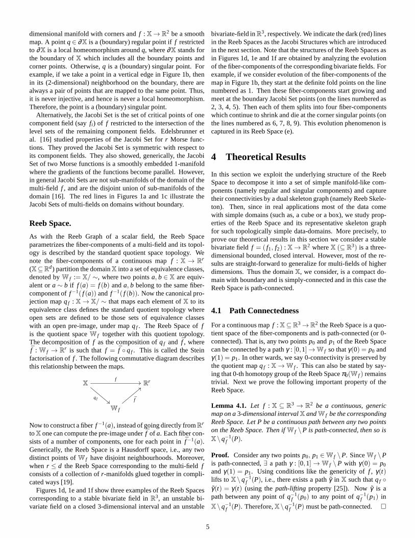
In this section we exploit the underlying structure of the ReebSpace to decompose it into a set of simple manifold-like com-ponents (namely regular and singular components) and capturetheir connectivities by a dual skeleton graph (namely Reeb Skele-ton). Then, since in real applications most of the data comewith simple domains (such as, a cube or a box), we study prop-erties of the Reeb Space and its representative skeleton graphfor such topologically simple data-domains. More precisely, toprove our theoretical results in this section we consider a stablebivariate field f = ( f1, f2) : X→ R2 whereX (⊆ R3) is a three-dimensional bounded, closed interval. However, most of there-sults are straight-forward to generalize for multi-fields of higherdimensions. Thus the domainX, we consider, is a compact do-main with boundary and is simply-connected and in this case theReeb Space is path-connected.
4.1 Path Connectedness
For a continuous mapf : X⊆ R3 →R2 the Reeb Space is a quo-tient space of the fiber-components and is path-connected (or 0-connected). That is, any two pointsp0 andp1 of the Reeb Spacecan be connected by a pathγ : [0,1]→W f so thatγ(0) = p0 andγ(1) = p1. In other wards, we say 0-connectivity is preserved bythe quotient mapqf : X → W f . This can also be stated by say-ing that 0-th homotopy group of the Reeb Spaceπ0(W f ) remainstrivial. Next we prove the following important property of theReeb Space.
Lemma 4.1. Let f : X ⊆ R3 → R2 be a continuous, genericmap on a3-dimensional intervalX andW f be the correspondingReeb Space. Let P be a continuous path between any two pointson the Reeb Space. Then ifW f \P is path-connected, then so isX\q−1
f (P).
Proof. Consider any two pointsp0, p1 ∈W f \P. SinceW f \Pis path-connected,∃ a pathγ : [0,1] → W f \P with γ(0) = p0
andγ(1) = p1. Using conditions like the genericity off , γ(t)lifts to X \q−1
f (P), i.e., there exists a pathγ in X such thatqf ◦
γ(t) = γ(t) (using thepath-lifting property [25]). Nowγ is apath between any point ofq−1
f (p0) to any point ofq−1f (p1) in
X\q−1f (P). Therefore,X\q−1
f (P) must be path-connected.�
5
Thus Lemma 4.1 implies if there exists a pathP in the Reeb Spacewhose preimageq−1
f (P) separates the domain thenP must alsoseparate the Reeb Space. This is a useful property in detachingunimportant components from the Reeb Space.
4.2 Jacobi Structure
As noted in Section 3, the Jacobi Set of a function is not the sameas the set of singular fibers, as each point in the Jacobi Set ismerely a representative of a singular fiber. Moreover, the struc-ture of the Reeb Space is actually given by a projection of theJacobi Set or the singular fibers. For example, in Figures 1c and1f, the Jacobi Set consists of 9 parallel lines in the domain,butthey correspond to 6 1-manifold structures in the Reeb Space.Note that if the input multi-field domain is with boundary, thereare additional edges (corresponding to the boundary JacobiSet)needed to describe the Reeb Space. We therefore introduce theJacobi Structure: the manifold structure of the Reeb Space cor-responding to the Jacobi Set in the domain.
Definition 4.1. TheJacobi Structure of a Reeb SpaceW f corre-sponding to a multi-field f: X⊆ R3 → R2 is denoted byJ f andis defined byJ f := qf (J f ), i.e., the projection of the Jacobi SetJ f to the Reeb Space by the quotient map qf : X→W f .
Note that according to our definition the Jacobi SetJ f consists ofboth the interior and the boundary Jacobi Set, i.e.,J f = J◦f ∪J∂
f .Thus each point of the Jacobi Structure corresponds to a singularfiber-component in the domainX of f , and vice-versa.
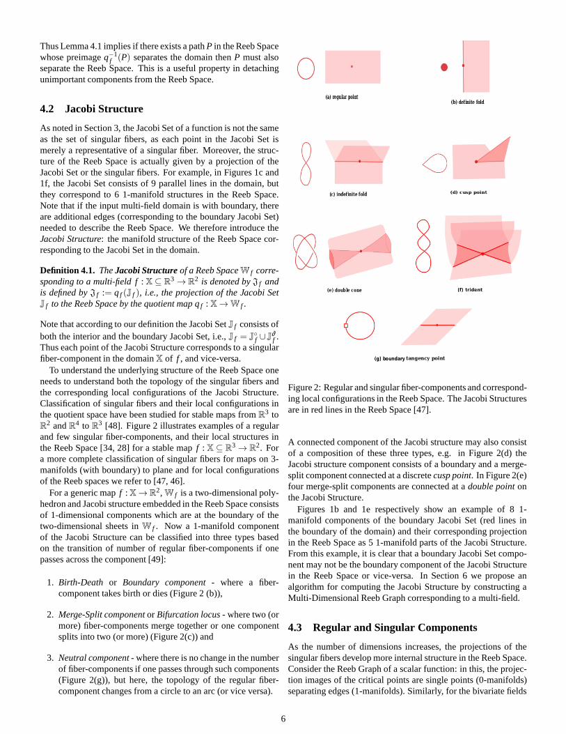
To understand the underlying structure of the Reeb Space oneneeds to understand both the topology of the singular fibers andthe corresponding local configurations of the Jacobi Structure.Classification of singular fibers and their local configurations inthe quotient space have been studied for stable maps fromR3 toR2 andR4 to R3 [48]. Figure 2 illustrates examples of a regularand few singular fiber-components, and their local structures inthe Reeb Space [34, 28] for a stable mapf : X ⊆ R3 → R2. Fora more complete classification of singular fibers for maps on 3-manifolds (with boundary) to plane and for local configurationsof the Reeb spaces we refer to [47, 46].
For a generic mapf : X→R2, W f is a two-dimensional poly-hedron and Jacobi structure embedded in the Reeb Space consistsof 1-dimensional components which are at the boundary of thetwo-dimensional sheets inW f . Now a 1-manifold componentof the Jacobi Structure can be classified into three types basedon the transition of number of regular fiber-components if onepasses across the component [49]:
1. Birth-Death or Boundary component- where a fiber-component takes birth or dies (Figure 2 (b)),
2. Merge-Split componentor Bifurcation locus- where two (ormore) fiber-components merge together or one componentsplits into two (or more) (Figure 2(c)) and
3. Neutral component- where there is no change in the numberof fiber-components if one passes through such components(Figure 2(g)), but here, the topology of the regular fiber-component changes from a circle to an arc (or vice versa).
Figure 2: Regular and singular fiber-components and correspond-ing local configurations in the Reeb Space. The Jacobi Structuresare in red lines in the Reeb Space [47].
A connected component of the Jacobi structure may also consistof a composition of these three types, e.g. in Figure 2(d) theJacobi structure component consists of a boundary and a merge-split component connected at a discretecusp point. In Figure 2(e)four merge-split components are connected at adouble pointonthe Jacobi Structure.
Figures 1b and 1e respectively show an example of 8 1-manifold components of the boundary Jacobi Set (red lines inthe boundary of the domain) and their corresponding projectionin the Reeb Space as 5 1-manifold parts of the Jacobi Structure.From this example, it is clear that a boundary Jacobi Set compo-nent may not be the boundary component of the Jacobi Structurein the Reeb Space or vice-versa. In Section 6 we propose analgorithm for computing the Jacobi Structure by constructing aMulti-Dimensional Reeb Graph corresponding to a multi-field.
4.3 Regular and Singular Components
As the number of dimensions increases, the projections of thesingular fibers develop more internal structure in the Reeb Space.Consider the Reeb Graph of a scalar function: in this, the projec-tion images of the critical points are single points (0-manifolds)separating edges (1-manifolds). Similarly, for the bivariate fields
6
shown in Figures 1d, 1e and 1f, the projections of the singu-lar fibers are arranged in a Reeb Space along 1-manifold curveswhich separate 2-manifold sheets. This induces a natural stratifi-cation or partition of the Reeb Space into disjoint subspaces (orstrata).
To describe a stratification of the Reeb Space and the corre-sponding domain of the multi-field we first classify the fiber-components of the generic mapf : X ⊆ R3 → R2 according totheir complexity or codimension of the subspace where they lie[49]. Given the Stein factorizationf = f ◦qf , fiber-componentsof f can be classified into three classes.
1. C0 = {q−1
f (s) : s ∈ W f andq−1f (s) does not contain any
singular point off}. Fiber-components of this class are theregular fiber-components and theirqf -images form codi-mension 0 subspaces inW f , denoted asW0
f .
2. C 1 = {q−1f (s) : s∈W f andq−1
f (s) contains exactly one de-finite or indefinite fold point}. Singular fiber-componentsof this class are moderately complex and theirqf -imagesform codimension 1 subspaces inW f , denoted asW1
f .
3. C 2 = {q−1f (s) : s ∈ W f andq−1
f (s) contains a cusp pointor two indefinite fold points}. Singular fiber-components ofthis class are the most complex and theirqf -images formcodimension 2 subspaces inW f , denoted asW2
f .
Complexity of a fiber-component increases as the codimensionof the corresponding subspace in the Reeb Space increases. Notethatqf -images of the fiber-components inC 1 andC 2 form the Ja-cobi StructureJ f of the Reeb Space, i.e.,J f =W1
f ∪W2f . Topo-
logically, regular fiber-components are either a circle or an arc[47]. For stable mapsf : X⊆R3 →R2, topologically there are 7different types of singular fibers inC 1 and 21 different types ofsingular fibers inC 2 [47].
Two regular pointsa, b ∈ W0f are topologically equivalentin
the Reeb SpaceW f or a∼ρ b if there exists a path betweena andb without intersecting the Jacobi StructureJ f . It is not difficult tocheck that ‘∼ρ ’ is an equivalence relation. Therefore, the equiv-alence relation ‘∼ρ ’ partitions the regular points ofW f into a setof equivalence classes. Now we prove that each such equivalenceclass is a 2-dimensional sheet.
Lemma 4.2(Partition ). The Jacobi structureJ f of a Reeb spaceW f corresponding to a smooth stable map f: X⊆R3 →R2 sep-arates the Reeb Space into a set of2-manifold components.
Proof. Let D be a small disk in the range consisting of regularvalues (i.e.,D does not intersectf (J f )). Then, by Ehresmann’sfibration theorem,f restricted tof−1(D) is equivalent to the pro-jection D×F → D, whereF is a 1-dimensional compact man-ifold. So, this means thatqf ( f−1(D)) can be identified with adisjoint union of some copies ofD, where the number of copiesis the same as the number of connected components ofF. EvenwhenD intersects withf (J f ), if we restrict f to the componentsof the inverse imagef−1(D) that do not intersectJ f , then thesame consequence holds. So, the regular sheets ofW f are lo-cally homeomorphic toD, and hence is a 2-manifold. �
Thus we have the following definition of regular components.
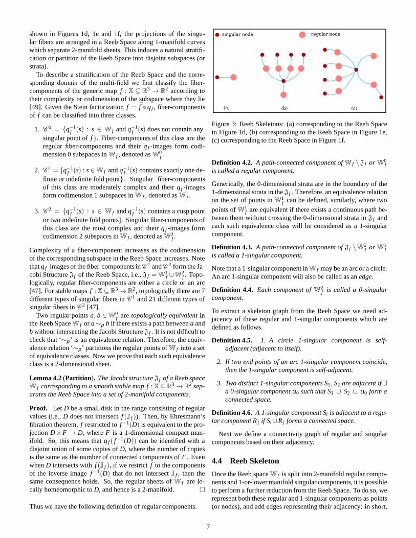
singular node regular node
(a) (b) (c)
Figure 3: Reeb Skeletons: (a) corresponding to the Reeb Spacein Figure 1d, (b) corresponding to the Reeb Space in Figure 1e,(c) corresponding to the Reeb Space in Figure 1f.
Definition 4.2. A path-connected component ofW f \J f or W0f
is called a regular component.
Generically, the 0-dimensional strata are in the boundary of the1-dimensional strata in theJ f . Therefore, an equivalence relationon the set of points inW1
f can be defined, similarly, where two
points ofW1f are equivalent if there exists a continuous path be-
tween them without crossing the 0-dimensional strata inJ f andeach such equivalence class will be considered as a 1-singularcomponent.
Definition 4.3. A path-connected component ofJ f \W2f or W1
fis called a 1-singular component.
Note that a 1-singular component inW f may be an arc or a circle.An arc 1-singular component will also be called as anedge.
Definition 4.4. Each component ofW2f is called a 0-singular
component.
To extract a skeleton graph from the Reeb Space we need ad-jacency of these regular and 1-singular components which aredefined as follows.
Definition 4.5. 1. A circle 1-singular component is self-adjacent (adjacent to itself).
2. If two end points of an arc 1-singular component coincide,then the 1-singular component is self-adjacent.
3. Two distinct 1-singular components S1, S2 are adjacent if∃a 0-singular componentα0 such that S1 ∪ S2 ∪ α0 form aconnected space.
Definition 4.6. A 1-singular component Si is adjacent to a regu-lar component Rj if Si ∪Rj forms a connected space.
Next we define a connectivity graph of regular and singularcomponents based on their adjacency.
4.4 Reeb Skeleton
Once the Reeb spaceW f is split into 2-manifold regular compo-nents and 1-or-lower manifold singular components, it is possibleto perform a further reduction from the Reeb Space. To do so, werepresent both these regular and 1-singular components as points(or nodes), and add edges representing their adjacency: in short,
7

Figure 4: (a) Reeb Space with self-adjacent 1-singular compo-nent (b) Corresponding Reeb Skeleton.
we can build the dual graph of these components of the ReebSpace. This has the merit of further reducing the Reeb Spacefrom a 2-dimensional structure to a fundamentally 1-dimensionalstructure which is easier to represent, to reason about and to vi-sualise. We refer to this as theReeb Skeletonand formally defineas follows.
Definition 4.7. Let R1,R2, . . . ,Rm be the regular components andS1,S2, . . . ,Sn be the 1-singular components ofW f . Then the ReebSkeleton of f , denoted byK f , is the adjacency graph which con-sists of (i) nodes nRi and nSj (i = 1,2, . . . ,m and j= 1,2, . . . ,n)corresponding to each of the regular and 1-singular components,and (ii) edges e(Sj ,Sj ′) and e(Ri ,Sj) that are defined as follows:
1. If Sj is self-adjacent, then e(Sj ,Sj) = 1. In other words, nSj
has a self-loop.
2. If Sj is self-adjacent and Sj is adjacent with a regular com-ponent Ri , then e(Ri ,Sj) = 2. In other words, nSj is con-nected with nRi by two edges.
3. If Sj and Sj ′ are two distinctnon-boundary 1-singular com-ponents, then
e(Sj ,Sj ′) =
{
1, if Sj , Sj ′ are adjacent0, otherwise.
4. For any regular component Ri and any 1-singular compo-nent Sj
e(Ri ,Sj) =
{
1, if Ri , Sj are adjacent0, otherwise.
The regular and 1-singular components of the Reeb Space arerepresented as theregularandsingular nodes, respectively, in theReeb Skeleton. Figure 3 shows some examples of Reeb Skele-tons corresponding to the Reeb Spaces in Figure 1. Figure 4 il-lustrates an example of the Reeb Skeleton with a self-adjacentsingular node. Note that although the Reeb Skeleton gives asimple abstraction of 0-connectivity in the Reeb Space, it losesinformation of higher-dimensional connectivities, like higher di-mensional holes (tunnels, voids) in the Reeb Space. But on theother hand, the Reeb Skeleton is extremely useful for extractingany “fork”-like structure (corresponding to a merge-splitfeature)in the Reeb Space. And we will see later by a little simplifica-tion we can extract the most prominent merge-split feature in theReeb Skeleton and so in the Reeb Space. Therefore, next westudy properties of the Reeb Skeleton to simplify it further.
Figure 5: Example of Reeb Space with a tunnel.
4.5 Simple Domains
We know from scalar fields that topologically simple domainshave a useful property: the Reeb Graph is guaranteed to be a tree- i.e. the contour tree. This not only enables more efficient com-putation, but also provides straightforward mechanisms for fea-ture extraction, simplification and visualisation. Ideally, in multi-fields, the Reeb Space would also be contractible to a point. Butwe show this is not true, in general.
In topology, simple domains are characterised bysimply-connected space. A topological space is simply-connected if itis path-connected and everyloop in that space can be continu-ously shrunk to a point without leaving the space. In terms ofhomotopy theory this means a simply-connected space is withoutany “handle-shaped hole” (as in Figure 5) or it has trivial funda-mental group. For example, a sphere (that has a hollow center)is a simply-connected space whereas a torus (that has a handle-shaped hole) is not. Even a simpler topological space is known ascontractible spacewhich is homotopically equivalent to a point.Note that a contractible space is simply-connected, but thecon-verse is not true. For example, a sphere is simply-connectedasevery loop on it can be contracted to a point on it, although thesphere is not a contractible space because of the center holeinit. In the following lemma, we prove that the Reeb Space cor-responding to a map defined on a simply-connected domain issimply-connected, but later we show it may not be contractible.
Lemma 4.3(Simply-Connected). The Reeb Space of a genericcontinuous map f: X⊆ R3 →R2 is simply-connected.
Proof. We consider any loop in the Reeb spaceW f . Then, it liftsto an arc inX. But, every fiber ofqf is connected, and therefore,it lifts to a loop. AsX is simply-connected, this lifted loop is null-homotopic. Therefore, itsqf -image is also null-homotopic fromthe continuity ofqf . This means thatW f is simply-connected.�
Therefore, if f is good enough (for example, triangulable orpiecewise linear), then the Reeb space is simply-connected. Thisimplies that the 1st homology of the Reeb Space also vanishes(oris the trivial group), and therefore the Reeb space does not havea tunnel or 1-dimensional hole (i.e., a hole inside a circleS1, e.g.Figure 5). Thus we have the following theorem.
Theorem 4.4.The Reeb Space of a generic map f:X⊆R3 →R2
does not contain any tunnel or1-dimensional hole.
On the other hand, for void or 2-dimensional hole (i.e., holeinside a sphereS2), this is no longer true. We can construct
8
xxxxxxxxxxxxxxxxxxxxxxxxxxxxxxxxxxxxxxxxxxxxxxxxxxxxxxxxxxxxxxxxxxxxxxxxxxxxxxxxxxxxxxxxxxxxxxxxxxxxxxxxxxxxxxxxxxxxxxxxxxxxxxxxxxxxxxxxxxxxxxxxxxxxxxxxxxxxxxxxxxxxxxxxxxxxxxxx
Figure 6: Reeb Space with a void.
a (piecewise linear) mapf : X → R2 whose Reeb space doeshave a 2-dimensional hole. For example, consider the Hopf fi-brationS3 → S2 and its composition with a standard projectionS2 → R2. The resulting mapS3 → R2 is not generic, but per-turbing it slightly along its Jacobi set, we can obtain a genericmapS3 → R2, whose Reeb space is the union of a 2-sphere andan annulus attached along the equator (and one boundary compo-nent of the annulus). Then, by extracting a 3-ball in the preimageof a two disk in the interior of the annulus part, we get the desiredmapX → R2. The Reeb space is the same space; the union ofS2 and an annulus (Figure 6). Over each blue point lies a point(definite fold) and it corresponds to a birth-death. Over each redpoint lies a fiber as in Figure 2(c) (with an indefinite fold) andthe splitting of a circle fiber occurs. Over each green point lies acircle touching the boundary of the domain cubeX. Thus, overeach point in the shaded disk bounded by the green circle liesaninterval. Note this disk is a subset of the annulus part. There-fore, a Reeb Space of a multi-field on a contractible domain maynot be contractible and simplification of such space may not besimple as in the scalar case.
According to Theorem 4.4, we can conclude that each regularcomponent ofW f is planar; i.e., each regular component is adisk possibly with holes. For example, torus with holes (or a1-dimensional hole as in Figure 5) never appears! This is essentialin applying our simplification rules for the Reeb Skeleton aswillbe discussed in Section 6.6 (Figure 11). Next we focus on findinga criterion for detachability of such regular components from theReeb Space for simplifying the corresponding the multi-field.
4.6 Detachability
In the case of scalar field in a simply-connected domain, the ReebSpace (Graph) is a contour tree and there always exists a leafedgethat can be detached in a mathematically correct way, unlessthecontour tree consists only of one edge. We find similar criteriafor definingdetachableregular components in the Reeb Space.
We say that it is possible to detach a regular component froma Reeb Space to obtain a simplified Reeb Space if the multi-fieldcorresponding to the initial Reeb Space could be simplified tothe multi-field corresponding to the modified one, and then theregular component is said to be detachable from the Reeb Space.Mathematically, any map could be simplified to a simpler mapin the following sense. SinceR2 is contractible, any two stable
maps f0 and f1 : X → R2 are homotopic. So, using singularitytheory, we can show thatf0 and f1 are connected by a generic1-parameter family of maps. So, if we take an arbitrary stablemap as f0 and a very simple map asf1, then f0 is simplifiedto f1 after the generic 1-parameter family. Such a 1-parameterfamily passes through finitely many bifurcation parameters, andsuch bifurcations can be classified [38].
Such transitions of the Reeb Spaces for generic smooth mapson a closed 3-dimensional manifold intoR2 have been studied in[38], although for maps on a 3-dimensional manifold with bound-ary these results need further extension. In the current paper, weconsider only a simple type of singularities and show that corre-sponding regular component is detachable from the Reeb Space.These components are known aslips and are defined as follows.
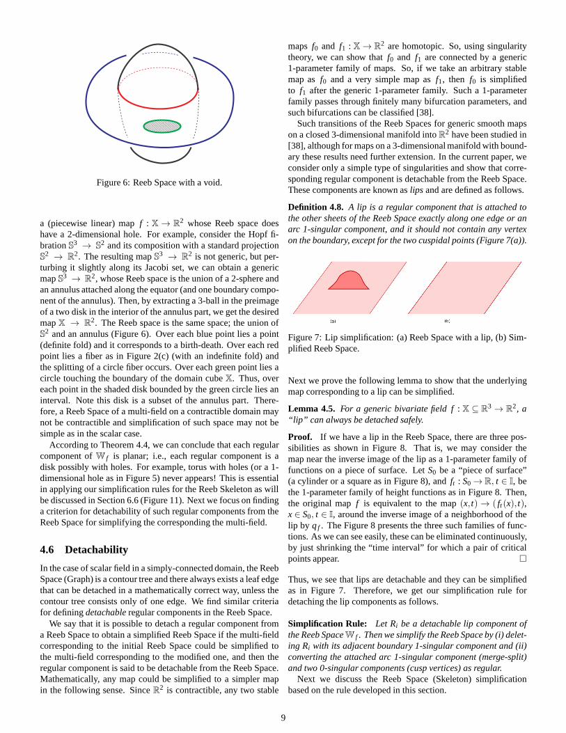
Definition 4.8. A lip is a regular component that is attached tothe other sheets of the Reeb Space exactly along one edge or anarc 1-singular component, and it should not contain any vertexon the boundary, except for the two cuspidal points (Figure 7(a)).
(a) (b)
Figure 7: Lip simplification: (a) Reeb Space with a lip, (b) Sim-plified Reeb Space.
Next we prove the following lemma to show that the underlyingmap corresponding to a lip can be simplified.
Lemma 4.5. For a generic bivariate field f: X ⊆ R3 → R2, a“lip” can always be detached safely.
Proof. If we have a lip in the Reeb Space, there are three pos-sibilities as shown in Figure 8. That is, we may consider themap near the inverse image of the lip as a 1-parameter family offunctions on a piece of surface. LetS0 be a “piece of surface”(a cylinder or a square as in Figure 8), andft : S0 → R, t ∈ I, bethe 1-parameter family of height functions as in Figure 8. Then,the original mapf is equivalent to the map(x, t) → ( ft (x), t),x∈ S0, t ∈ I, around the inverse image of a neighborhood of thelip by qf . The Figure 8 presents the three such families of func-tions. As we can see easily, these can be eliminated continuously,by just shrinking the “time interval” for which a pair of criticalpoints appear. �
Thus, we see that lips are detachable and they can be simplifiedas in Figure 7. Therefore, we get our simplification rule fordetaching the lip components as follows.
Simplification Rule: Let Ri be a detachable lip component ofthe Reeb SpaceW f . Then we simplify the Reeb Space by (i) delet-ing Ri with its adjacent boundary 1-singular component and (ii)converting the attached arc 1-singular component (merge-split)and two 0-singular components (cusp vertices) as regular.
Next we discuss the Reeb Space (Skeleton) simplificationbased on the rule developed in this section.
9
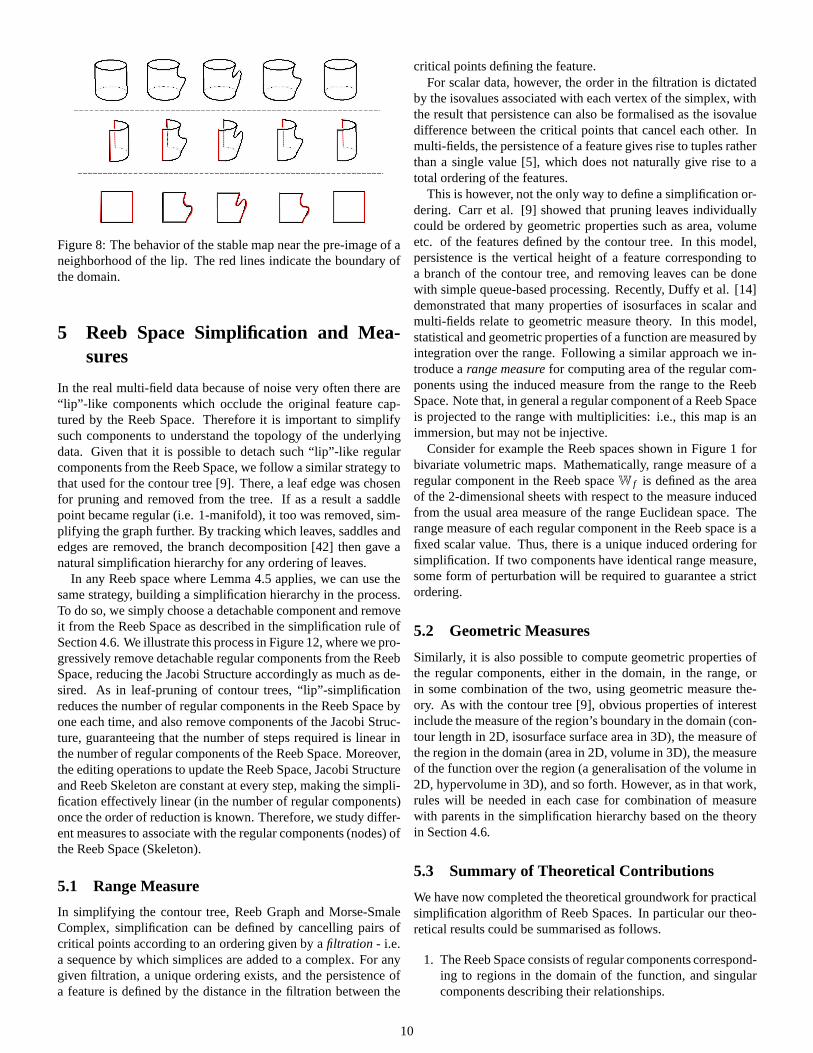
Figure 8: The behavior of the stable map near the pre-image ofaneighborhood of the lip. The red lines indicate the boundaryofthe domain.
5 Reeb Space Simplification and Mea-sures
In the real multi-field data because of noise very often thereare“lip”-like components which occlude the original feature cap-tured by the Reeb Space. Therefore it is important to simplifysuch components to understand the topology of the underlyingdata. Given that it is possible to detach such “lip”-like regularcomponents from the Reeb Space, we follow a similar strategytothat used for the contour tree [9]. There, a leaf edge was chosenfor pruning and removed from the tree. If as a result a saddlepoint became regular (i.e. 1-manifold), it too was removed,sim-plifying the graph further. By tracking which leaves, saddles andedges are removed, the branch decomposition [42] then gave anatural simplification hierarchy for any ordering of leaves.
In any Reeb space where Lemma 4.5 applies, we can use thesame strategy, building a simplification hierarchy in the process.To do so, we simply choose a detachable component and removeit from the Reeb Space as described in the simplification ruleofSection 4.6. We illustrate this process in Figure 12, where we pro-gressively remove detachable regular components from the ReebSpace, reducing the Jacobi Structure accordingly as much asde-sired. As in leaf-pruning of contour trees, “lip”-simplificationreduces the number of regular components in the Reeb Space byone each time, and also remove components of the Jacobi Struc-ture, guaranteeing that the number of steps required is linear inthe number of regular components of the Reeb Space. Moreover,the editing operations to update the Reeb Space, Jacobi Structureand Reeb Skeleton are constant at every step, making the simpli-fication effectively linear (in the number of regular components)once the order of reduction is known. Therefore, we study differ-ent measures to associate with the regular components (nodes) ofthe Reeb Space (Skeleton).
5.1 Range Measure
In simplifying the contour tree, Reeb Graph and Morse-SmaleComplex, simplification can be defined by cancelling pairs ofcritical points according to an ordering given by afiltration - i.e.a sequence by which simplices are added to a complex. For anygiven filtration, a unique ordering exists, and the persistence ofa feature is defined by the distance in the filtration between the
critical points defining the feature.For scalar data, however, the order in the filtration is dictated
by the isovalues associated with each vertex of the simplex,withthe result that persistence can also be formalised as the isovaluedifference between the critical points that cancel each other. Inmulti-fields, the persistence of a feature gives rise to tuples ratherthan a single value [5], which does not naturally give rise toatotal ordering of the features.
This is however, not the only way to define a simplification or-dering. Carr et al. [9] showed that pruning leaves individuallycould be ordered by geometric properties such as area, volumeetc. of the features defined by the contour tree. In this model,persistence is the vertical height of a feature corresponding toa branch of the contour tree, and removing leaves can be donewith simple queue-based processing. Recently, Duffy et al.[14]demonstrated that many properties of isosurfaces in scalarandmulti-fields relate to geometric measure theory. In this model,statistical and geometric properties of a function are measured byintegration over the range. Following a similar approach wein-troduce arange measurefor computing area of the regular com-ponents using the induced measure from the range to the ReebSpace. Note that, in general a regular component of a Reeb Spaceis projected to the range with multiplicities: i.e., this map is animmersion, but may not be injective.
Consider for example the Reeb spaces shown in Figure 1 forbivariate volumetric maps. Mathematically, range measureof aregular component in the Reeb spaceW f is defined as the areaof the 2-dimensional sheets with respect to the measure inducedfrom the usual area measure of the range Euclidean space. Therange measure of each regular component in the Reeb space is afixed scalar value. Thus, there is a unique induced ordering forsimplification. If two components have identical range measure,some form of perturbation will be required to guarantee a strictordering.
5.2 Geometric Measures
Similarly, it is also possible to compute geometric properties ofthe regular components, either in the domain, in the range, orin some combination of the two, using geometric measure the-ory. As with the contour tree [9], obvious properties of interestinclude the measure of the region’s boundary in the domain (con-tour length in 2D, isosurface surface area in 3D), the measure ofthe region in the domain (area in 2D, volume in 3D), the measureof the function over the region (a generalisation of the volume in2D, hypervolume in 3D), and so forth. However, as in that work,rules will be needed in each case for combination of measurewith parents in the simplification hierarchy based on the theoryin Section 4.6.
5.3 Summary of Theoretical Contributions
We have now completed the theoretical groundwork for practicalsimplification algorithm of Reeb Spaces. In particular our theo-retical results could be summarised as follows.
1. The Reeb Space consists of regular components correspond-ing to regions in the domain of the function, and singularcomponents describing their relationships.
10
2. The Jacobi Set in the domain does not capture all of thestructure of the singular components in the Reeb Space, andthe Jacobi Structure is needed to do so.
3. The Jacobi Structure of the Reeb Space can be used to fur-ther collapse the Reeb Space into the Reeb Skeleton.
4. Multifields with topologically simple domains can be sim-plified using a variation on the leaf-pruning used for contourtrees.
5. A Reeb Space measure and other geometric measures areintroduced to guide the Reeb Space simplification process.
We now turn to the practical and algorithmic part of this paper:how to simplify the Joint Contour Net, an approximation of theReeb Space.
6 Algorithm: Simplifying the Joint Con-tour Net
In this section, first we introduce the Joint Contour Net, a graphdata-structure that approximates the Reeb Space. As describedin [7], the Joint Contour Net is a quantized approximation oftheReeb Space. Therefore, to avoid having duplicate terminologywe will use the same terminology for JCN as what we have de-veloped for the Reeb Space, namely, Jacobi Structure, RegularComponent, Singular Components, Reeb Skeleton etc.
6.1 Joint Contour Net
The Joint Contour Net (JCN) [7, 15] approximates the ReebSpaceW f of a multi-field f = ( f1, f2, . . . , fr) : X ⊂ Rd → Rr
in a d-dimensional intervalX. Let f = ( f1, f2, . . . , fr) : M → Rr
be a piecewise-linear (PL) approximation off corresponding to ameshM of X. The idea of computing the JCN is based on quanti-zation of the fiber-components off . The JCN f with a quantiza-tion level (or level of resolution)mQ is denoted asJCN( f ,mQ),wheremQ refers to how fine the rectangular mesh for the rangeis.
A quantized level setof fi at an isovalueh ∈ Z/mQ is de-noted by Qf−1
i (h) and is defined as:Qf−1i (h) :=
{
x ∈ M :( 1
mQ) round(mQ fi(x)) = h}. A connected component of the quan-
tized level set in the mesh is called aquantized contouror acon-tour slab. The part of the contour slab in a single cell of the meshis called acontour fragment.
Now the first step of the JCN algorithm constructs all the con-tour fragments corresponding to a quantization of each compo-nent field. In the second step, thejoint contour fragmentsarecomputed by computing the intersections of these contour frag-ments for the component fields in a cell. The third step is to con-struct an adjacency graph of these joint contour fragments wherea node in the graph corresponds to a joint contour fragment andthere is an edge between two nodes if the corresponding jointcontour fragments are adjacent. Finally, the JCN is obtained bycollapsing the neighbouring redundant nodes with identical iso-values. Thus, each node in the JCN corresponds to ajoint contourslab (or quantized fiber-component) and an edge represents theadjacency between two quantized fiber-components (with quan-tization levelmQ) of f .
(0,0) (3,2)
(5,0)
(5,0)
k
i l
l
i
f
d
e
c
b
a0,0
1,01,1
2,1 2,2
3,2
2,0
3,03,1
4,14,0
2,0
3,0 3,1
4,0 4,1
5,0
1,0
1,1
2,1
2,2
2,0 2,0
4,0
5,04,1
4,0
4,1
3,03,0
3,1 3,1
3,2
a b c d e f
g
g
h
h
i
i
j
j
k
l
0,0 1,0 1,1 2,1 2,2 3,2
2,0
3,0
3,1
4,1
4,0
5,0
2,0
3,0
3,1
4,0
4,1
5,0
Figure 9: (top) The joint contour fragments and their ad-jacency graph for a PL-bivariate field defined by the values{(5,0),(0,0),(5,0),(3,2)} at the vertices of a mesh of two trian-gles. (middle) The Multi-Dimensional Reeb Graph constructedfrom the JCN. The critical nodes of the MDRG are the ‘red’nodes which form the Jacobi Structure. (bottom) CorrespondingJoint Contour Net, with critical nodes from the MDRG markedin colour.
11
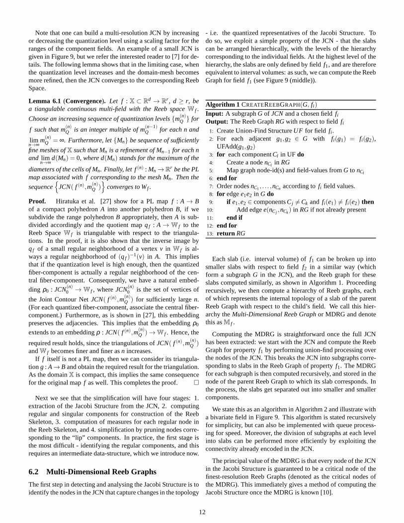
Note that one can build a multi-resolution JCN by increasingor decreasing the quantization level using a scaling factorfor theranges of the component fields. An example of a small JCN isgiven in Figure 9, but we refer the interested reader to [7] for de-tails. The following lemma shows that in the limiting case, whenthe quantization level increases and the domain-mesh becomesmore refined, then the JCN converges to the corresponding ReebSpace.
Lemma 6.1 (Convergence). Let f : X ⊂ Rd → Rr , d ≥ r, bea tiangulable continuous multi-field with the Reeb spaceW f .
Choose an increasing sequence of quantization levels{m(n)Q } for
f such that m(n)Q is an integer multiple of m(n−1)Q for each n and
limn→∞
m(n)Q = ∞. Furthermore, let{Mn} be sequence of sufficiently
fine meshes ofX such that Mn is a refinement of Mn−1 for each nand lim
n→∞d(Mn) = 0, where d(Mn) stands for the maximum of the
diameters of the cells of Mn. Finally, let f(n) : Mn →Rr be the PLmap associated with f corresponding to the mesh Mn. Then the
sequence{
JCN( f (n),m(n)Q )
}
converges to Wf .
Proof. Hiratuka et al. [27] show for a PL mapf : A → Bof a compact polyhedronA into another polyhedronB, if wesubdivide the range polyhedronB appropriately, thenA is sub-divided accordingly and the quotient mapqf : A → W f to theReeb SpaceW f is triangulable with respect to the triangula-tions. In the proof, it is also shown that the inverse image byqf of a small regular neighborhood of a vertexv in W f is al-ways a regular neighborhood of(qf )
−1(v) in A. This impliesthat if the quantization level is high enough, then the quantizedfiber-component is actually a regular neighborhood of the cen-tral fiber-component. Consequently, we have a natural embed-
ding ρ0 : JCN(n)0 → W f , whereJCN(n)
0 is the set of vertices of
the Joint Contour NetJCN( f (n),m(n)Q ) for sufficiently largen.
(For each quantized fiber-component, associate the centralfiber-component.) Furthermore, as is shown in [27], this embeddingpreserves the adjacencies. This implies that the embeddingρ0
extends to an embeddingρ : JCN( f (n),m(n)Q )→W f . Hence, the
required result holds, since the triangulations ofJCN( f (n),m(n)Q )
andW f becomes finer and finer asn increases.If f itself is not a PL map, then we can consider its triangula-
tion g : A→B and obtain the required result for the triangulation.As the domainX is compact, this implies the same consequencefor the original mapf as well. This completes the proof. �
Next we see that the simplification will have four stages: 1.extraction of the Jacobi Structure from the JCN, 2. computingregular and singular components for construction of the ReebSkeleton, 3. computation of measures for each regular node inthe Reeb Skeleton, and 4. simplification by pruning nodes corre-sponding to the “lip” components. In practice, the first stage isthe most difficult - identifying the regular components, andthisrequires an intermediate data-structure, which we introduce now.
6.2 Multi-Dimensional Reeb Graphs
The first step in detecting and analysing the Jacobi Structure is toidentify the nodes in the JCN that capture changes in the topology
- i.e. the quantized representatives of the Jacobi Structure. Todo so, we exploit a simple property of the JCN - that the slabscan be arranged hierarchically, with the levels of the hierarchycorresponding to the individual fields. At the highest levelof thehierarchy, the slabs are only defined by fieldf1, and are thereforeequivalent to interval volumes: as such, we can compute the ReebGraph for fieldf1 (see Figure 9 (middle)).
Algorithm 1 CREATEREEBGRAPH(G, fi)Input: A subgraphG of JCN and a chosen fieldfiOutput: The Reeb GraphRGwith respect to fieldfi
1: Create Union-Find StructureUF for field fi .2: For each adjacentg1,g2 ∈ G with fi(g1) = fi(g2),
UFAdd(g1,g2)3: for each componentCl in UF do4: Create a nodenCl in RG5: Map graph node-id(s) and field-values fromG to nCl
6: end for7: Order nodesnC1, . . . ,nCn according tofi field values.8: for edgee1e2 in G do9: if e1,e2 ∈ componentsCj 6=Ck and fi(e1) 6= fi(e2) then
10: Add edgee(nCj ,nCk) in RG if not already present11: end if12: end for13: return RG
Each slab (i.e. interval volume) off1 can be broken up intosmaller slabs with respect to fieldf2 in a similar way (whichform a subgraphG in the JCN), and the Reeb graph for theseslabs computed similarly, as shown in Algorithm 1. Proceedingrecursively, we then compute a hierarchy of Reeb graphs, eachof which represents the internal topology of a slab of the parentReeb Graph with respect to the child’s field. We call this hier-archy theMulti-Dimensional Reeb Graphor MDRG and denotethis asM f .
Computing the MDRG is straightforward once the full JCNhas been extracted: we start with the JCN and compute the ReebGraph for propertyf1 by performing union-find processing overthe nodes of the JCN. This breaks the JCN into subgraphs corre-sponding to slabs in the Reeb Graph of propertyf1. The MDRGfor each subgraph is then computed recursively, and stored in thenode of the parent Reeb Graph to which its slab corresponds. Inthe process, the slabs get separated out into smaller and smallercomponents.
We state this as an algorithm in Algorithm 2 and illustrate witha bivariate field in Figure 9. This algorithm is stated recursivelyfor simplicity, but can also be implemented with queue process-ing for speed. Moreover, the division of subgraphs at each levelinto slabs can be performed more efficiently by exploiting theconnectivity already encoded in the JCN.
The principal value of the MDRG is that every node of the JCNin the Jacobi Structure is guaranteed to be a critical node ofthefinest-resolution Reeb Graphs (denoted as the critical nodes ofthe MDRG). This immediately gives a method of computing theJacobi Structure once the MDRG is known [10].
12
Algorithm 2 MULTI DIMENSIONALREEBGRAPH(G, fi , . . . , fr)Input: GraphG, fields fi , . . . , fr Output: MDRG M
1: if i ≤ r then2: Let R= CreateReebGraph(G, fi)3: StoreRas root node ofM4: for Each slabsof Rdo5: Extract subgraphGs of nodes ofG belonging tos in
R6: Compute Ms = MultiDimensionalReebGraph(Gs, fi+1,
. . . , fr )7: StoreMs at nodes of R8: end for9: return M
10: else11: return M = /012: end if
6.3 Jacobi Structure Extraction
Since every node belonging to the Jacobi Structure is guaranteedto appear as a critical node of the lowest level of an MDRG, theinitial stage in Jacobi Structure extraction is simply to mark thesenodes. Unmarked nodes are then guaranteed to be regular, andcan be collected into regular components. Once this has beendone, any remaining nodes that are adjacent to each other andtothe same set of regular components are identified, as these forma 1-singular component between the regular components.
The first stage of this can be seen in Figure 9, where the criticalnodes of the lowest level of the MDRG together mark all of theJacobi Structure nodes in the JCN (in colour).
6.4 Reeb Skeleton Construction
Once we have extracted the Jacobi Structure for the JCN, it isstraightforward to compute the corresponding Reeb Skeleton bycreating a single node for each regular or 1-singular component,and connecting them using the adjacency of components in theJacobi Structure. In Figure 6.4 we see an example of the ReebSkeleton construction for a volumetric bivariate field. We note,in this case, the Reeb Skeleton has no detachable lip-like regularnode whereas the Reeb Skeleton Figure 12 (d) has such detach-able nodes.
Now in the simplification algorithm, the order in which de-tachable Reeb Skeleton nodes are removed is determined by themetrics associated with those nodes. Computation of such met-rics are described next.
6.5 Computing Simplification Metrics
Our simplification algorithm can use any desired measure of im-portance for components of the Reeb space, including but notlimited to:
• Range measure.As described in Subsection 5.1, we canmeasure the size of the regular components by the inducedmeasure of the range. This is easy to approximate - in thiscase, by the number of unique JCN slabs (i.e. pixels in therange) that map to a given regular component.
(a) (b)
(c)
1
2
3
4
5
6
7
8
9
10
(d)
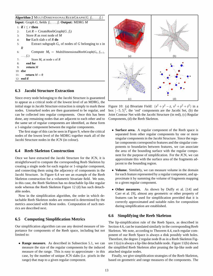
Figure 10: (a) Bivariate Field:(x2 + y2 − z, x2 + y2 + z2) in abox [−5, 5]3, the ‘red’ components are the Jacobi Set, (b) theJoint Contour Net with the Jacobi Structure (in red), (c) RegularComponents, (d) the Reeb Skeleton.
• Surface area. A regular component of the Reeb space isseparated from other regular components by one or moresingular components in the Jacobi Structure. Since the regu-lar components correspond to features and the singular com-ponents to boundaries between features, we can associatethe area of the bounding surface with the regular compo-nent for the purpose of simplification. For the JCN, we canapproximate this with the surface area of the fragments ad-jacent to the bounding region.
• Volume. Similarly, we can measure volume in the domainfor each feature represented by a regular component, and ap-proximate it by summing the volume of fragments mappingto a given regular component.
• Other measures. As shown by Duffy et al. [14] andCarr et al. [9], almost any geometric or other property offeatures can be used for simplification provided that it iscorrectly approximated and suitable rules for compositionduring simplification are established.
6.6 Simplifying the Reeb Skeleton
The lip-simplification rule of the Reeb Space, as described inSection 4.6, can be translated similarly in the corresponding ReebSkeleton. We note, according to Theorem 4.4, each regular com-ponent of our Reeb Space is always a disk possibly with holes.Therefore, the degree 2 regular node B as in a Reeb Skeleton Fig-ure 11(a) is always a lip-like detachable node. Figure 11(b)showsthe simplified Reeb Skeleton after pruning the lip-like nodeandattached singular nodes.
Finally, we give simplification strategies of the Reeb Skeleton,based on geometric and range measures of the components. The
13
Algorithm 3 SIMPLIFY REEBSPACE
Input: JCNJCNOutput: Reeb SkeletonK f
1: Build MDRG M f and Jacobi StructureJ f from JCNJCN.2: Partition JCNinto disjoint regular components
C= {R1, . . . ,Rm} by deletingJ f from JCN.3: PartitionJ f into disjoint 1-singular components{S1, . . . ,Sn}
based on adjacency to regular components inC.4: Use adjacencies of{R1, . . . ,Rm,S1, . . . ,Sn} to constructK f
(following defintion 4.7).5: Push “detachable” nodes ofK f on priority queuePQ with
priority determined by geometric measures.6: while PQ not empty (or priority is below a threshold value)
do7: Pop noder from queue8: Pruner fromK f
9: end while10: return Simplified Reeb SkeletonK f .
(�)
���
B
A
A
"����-pruning
Figure 11: Simplification rule for detaching a lip-like node(reg-ular node B in (a)) from the Reeb skeleton.
Reeb skeleton simplification method simplifies the Reeb skeletonand the corresponding Reeb space given a threshold (between0 and 1) adapting the previous approaches in the literature [6,54]. The threshold represents a “scale”, under which detachableregular nodes of the Reeb skeleton are considered as unimportant(noise). The threshold is expressed as a fraction of the rangeof the metric used. It can vary from 0 (no simplification) to 1(maximal simplification).
Figure 12 demonstrates the simplification of components fromthe Reeb Space, of an unstable bivariate volumetric data. Weuse range measure for ordering the components. We note, regu-lar nodes 4 and 2 in Figure 12 are not strictly the lips accordingto our definition of lips. However, a perturbation can be appliedfirst to convert such components to lips and then lip simplifica-tions can be applied. In Figure 12 we apply our lip-simplificationrule directly at the regular nodes 4 and 2, sequentially (node with
Figure 12: (Simplification Demo) (a) Original JCN/Reeb Spaceof bivariate field (Paraboloid, Height) (b) Jacobi Structure, (c)Regular components (d) Reeb Skeleton (‘blue’ corresponds toregular components and ‘red’ corresponds to adjacent 1-singularcomponents) (e) Simplified JCN (f)-(g) Simplified Reeb Skeletonusing range measure.
smaller measure is pruned first).
7 Implementation and Application
We implement our Reeb Space or JCN simplification algorithmusing the Visualization Toolkit (VTK) [1]. Details of the JCNimplementation can be found in [7, 15]. Our Reeb Space sim-plification implementation takes the JCN (a vtkGraph structure)as input and builds four filters: (1) The first filter computes theJacobi Structure by implementing the Multi-dimensional Reebgraph algorithm, (2) The second filter builds the Reeb Skeletonstructure by partitioning the JCN, (3) The third filter implementspersistence and geometric measures and (4) The fourth filterim-plements the simplification rules of the Reeb Skeleton. We usea vtkTree structure to store the Multi-Dimensional Reeb Graph(MDRG): Reeb graphs at each level of MDRG are stored in avtkReebGraph structure. For capturing the Reeb skeleton weuse
14
the vtkGraph structure.
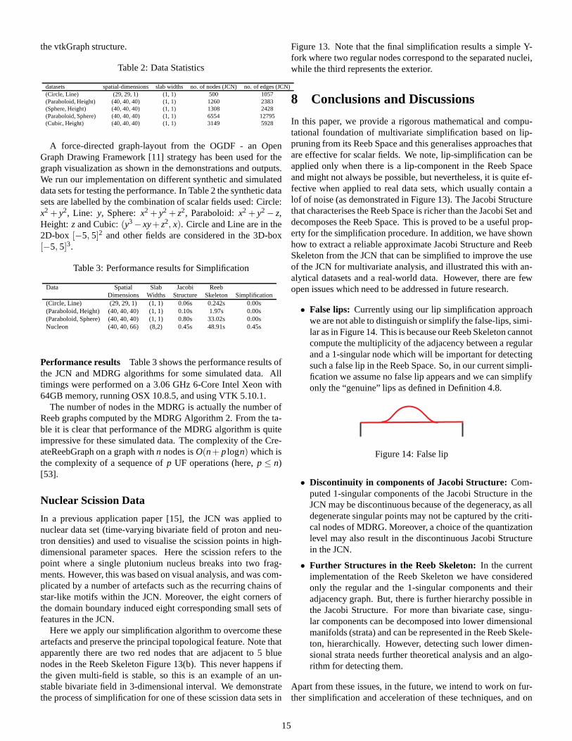
Table 2: Data Statistics
datasets spatial-dimensions slab widths no. of nodes (JCN)no. of edges (JCN)(Circle, Line) (29, 29, 1) (1, 1) 500 1057(Paraboloid, Height) (40, 40, 40) (1, 1) 1260 2383(Sphere, Height) (40, 40, 40) (1, 1) 1308 2428(Paraboloid, Sphere) (40, 40, 40) (1, 1) 6554 12795(Cubic, Height) (40, 40, 40) (1, 1) 3149 5928
A force-directed graph-layout from the OGDF - an OpenGraph Drawing Framework [11] strategy has been used for thegraph visualization as shown in the demonstrations and outputs.We run our implementation on different synthetic and simulateddata sets for testing the performance. In Table 2 the synthetic datasets are labelled by the combination of scalar fields used: Circle:x2 + y2, Line: y, Sphere:x2 + y2 + z2, Paraboloid:x2 + y2 − z,Height: z and Cubic:(y3− xy+ z2, x). Circle and Line are in the2D-box [−5, 5]2 and other fields are considered in the 3D-box[−5, 5]3.
Table 3: Performance results for Simplification
Data Spatial Slab Jacobi ReebDimensions Widths Structure Skeleton Simplification
(Circle, Line) (29, 29, 1) (1, 1) 0.06s 0.242s 0.00s(Paraboloid, Height) (40, 40, 40) (1, 1) 0.10s 1.97s 0.00s(Paraboloid, Sphere) (40, 40, 40) (1, 1) 0.80s 33.02s 0.00sNucleon (40, 40, 66) (8,2) 0.45s 48.91s 0.45s
Performance results Table 3 shows the performance results ofthe JCN and MDRG algorithms for some simulated data. Alltimings were performed on a 3.06 GHz 6-Core Intel Xeon with64GB memory, running OSX 10.8.5, and using VTK 5.10.1.
The number of nodes in the MDRG is actually the number ofReeb graphs computed by the MDRG Algorithm 2. From the ta-ble it is clear that performance of the MDRG algorithm is quiteimpressive for these simulated data. The complexity of the Cre-ateReebGraph on a graph withn nodes isO(n+ plogn) which isthe complexity of a sequence ofp UF operations (here,p ≤ n)[53].
Nuclear Scission Data
In a previous application paper [15], the JCN was applied tonuclear data set (time-varying bivariate field of proton andneu-tron densities) and used to visualise the scission points inhigh-dimensional parameter spaces. Here the scission refers to thepoint where a single plutonium nucleus breaks into two frag-ments. However, this was based on visual analysis, and was com-plicated by a number of artefacts such as the recurring chains ofstar-like motifs within the JCN. Moreover, the eight corners ofthe domain boundary induced eight corresponding small setsoffeatures in the JCN.
Here we apply our simplification algorithm to overcome theseartefacts and preserve the principal topological feature.Note thatapparently there are two red nodes that are adjacent to 5 bluenodes in the Reeb Skeleton Figure 13(b). This never happens ifthe given multi-field is stable, so this is an example of an un-stable bivariate field in 3-dimensional interval. We demonstratethe process of simplification for one of these scission data sets in
Figure 13. Note that the final simplification results a simpleY-fork where two regular nodes correspond to the separated nuclei,while the third represents the exterior.
8 Conclusions and Discussions
In this paper, we provide a rigorous mathematical and compu-tational foundation of multivariate simplification based on lip-pruning from its Reeb Space and this generalises approachesthatare effective for scalar fields. We note, lip-simplificationcan beapplied only when there is a lip-component in the Reeb Spaceand might not always be possible, but nevertheless, it is quite ef-fective when applied to real data sets, which usually contain alof of noise (as demonstrated in Figure 13). The Jacobi Structurethat characterises the Reeb Space is richer than the Jacobi Set anddecomposes the Reeb Space. This is proved to be a useful prop-erty for the simplification procedure. In addition, we have shownhow to extract a reliable approximate Jacobi Structure and ReebSkeleton from the JCN that can be simplified to improve the useof the JCN for multivariate analysis, and illustrated this with an-alytical datasets and a real-world data. However, there arefewopen issues which need to be addressed in future research.
• False lips: Currently using our lip simplification approachwe are not able to distinguish or simplify the false-lips, simi-lar as in Figure 14. This is because our Reeb Skeleton cannotcompute the multiplicity of the adjacency between a regularand a 1-singular node which will be important for detectingsuch a false lip in the Reeb Space. So, in our current simpli-fication we assume no false lip appears and we can simplifyonly the “genuine” lips as defined in Definition 4.8.
Figure 14: False lip
• Discontinuity in components of Jacobi Structure: Com-puted 1-singular components of the Jacobi Structure in theJCN may be discontinuous because of the degeneracy, as alldegenerate singular points may not be captured by the criti-cal nodes of MDRG. Moreover, a choice of the quantizationlevel may also result in the discontinuous Jacobi Structurein the JCN.
• Further Structures in the Reeb Skeleton: In the currentimplementation of the Reeb Skeleton we have consideredonly the regular and the 1-singular components and theiradjacency graph. But, there is further hierarchy possible inthe Jacobi Structure. For more than bivariate case, singu-lar components can be decomposed into lower dimensionalmanifolds (strata) and can be represented in the Reeb Skele-ton, hierarchically. However, detecting such lower dimen-sional strata needs further theoretical analysis and an algo-rithm for detecting them.
Apart from these issues, in the future, we intend to work on fur-ther simplification and acceleration of these techniques, and on
15
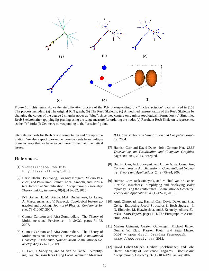
(a) (b) (c)
(d) (e) (f)
Figure 13: This figure shows the simplification process of theJCN corresponding to a “nuclear scission” data set used in [15].The process includes: (a) The original JCN graph; (b) The Reeb Skeleton; (c) A modified representation of the Reeb Skeleton bychanging the colour of the degree 2 singular nodes as “blue”,since they capture only minor topological information, (d)SimplifiedReeb Skeleton after applying lip-pruning using the range measure for ordering the nodes (e) Resultant Reeb Skeleton is representedas the “Y”-fork; (f) Geometry corresponding to the “scission” point.
alternate methods for Reeb Space computation and / or approxi-mation. We also expect to examine more data sets from multipledomains, now that we have solved more of the main theoreticalissues.
References
[1] Visualization Toolkit.http://www.vtk.org/, 2013.
[2] Harsh Bhatia, Bei Wang, Gregory Norgard, Valerio Pas-cucci, and Peer-Timo Bremer. Local, Smooth, and Consis-tent Jacobi Set Simplification.Computational Geometry:Theory and Applications, 48(4):311–332, 2015.
[3] P-T Bremer, E. M. Bringa, M.A. Duchaineau, D. Laney,A. Mascarenhas, and V. Pascucci. Topological feature ex-traction and tracking.Journal of Physics: Conference Se-ries, 78:012007, 2007.
[4] Gunnar Carlsson and Afra Zomorodian. The Theory ofMultidimensional Persistence. InSoCG, pages 71–93,2007.
[5] Gunnar Carlsson and Afra Zomorodian. The Theory ofMultidimensional Persistence.Discrete and ComputationalGeometry - 23rd Annual Symposium on Computational Ge-ometry, 42(1):71–93, 2009.
[6] H. Carr, J. Snoeyink, and M. van de Panne. Simplify-ing Flexible Isosurfaces Using Local Geometric Measures.
IEEE Transactions on Visualization and Computer Graph-ics, 2004.
[7] Hamish Carr and David Duke. Joint Contour Net.IEEETransactions on Visualization and Computer Graphics,pages xxx–xxx, 2013. accepted.
[8] Hamish Carr, Jack Snoeyink, and Ulrike Axen. ComputingContour Trees in All Dimensions.Computational Geome-try: Theory and Applications, 24(2):75–94, 2003.
[9] Hamish Carr, Jack Snoeyink, and Michiel van de Panne.Flexible isosurfaces: Simplifying and displaying scalartopology using the contour tree.Computational Geometry:Theory and Applications, 43(1):42–58, 2010.
[10] Amit Chattopadhyay, Hamish Carr, David Duke, and ZhaoGeng. Extracting Jacobi Structures in Reeb Spaces. InN. Elmqvist, M. Hlawitschka, and J. Kennedy, editors,Eu-roVis - Short Papers, pages 1–4. The Eurographics Associ-ation, 2014.
[11] Markus Chimani, Carsten Gutwenger, Michael Junger,Gunnar W. Klau, Karsten Klein, and Petra Mutzel.OGDF - Open Graph Drawing Framework.http://www.ogdf.net/, 2012.
[12] David Cohen-Steiner, Herbert Edelsbrunner, and JohnHarer. Stability of Persistence Diagrams.Discrete andComputational Geometry, 37(1):103–120, January 2007.
16

[13] Tamal K. Dey, Herbert Edelsbrunner, Sumanta Guha, andDmitry V. Nekhayev. Topology preserving edge contrac-tion. Publ. Inst. Math. (Beograd) (N.S), 66:23–45, 1998.
[14] Brian Duffy, Hamish Carr, and Torsten Moller. IntegratingIsosurface Statistics and Histograms.IEEE Transactionson Visualization and Computer Graphics, 19(2):263–277,2012.
[15] David Duke, Hamish Carr, Nicolas Schunck, Hai AhNam, and Andrzej Staszczak. Visualizing nuclear scis-sion through a multifield extension of topological analysis.IEEE Transactions on Visualization and Computer Graph-ics, 18(12):2033–2040, 2012.
[16] Herbert Edelsbrunner and John Harer. Jacobi Sets of Mul-tiple Morse Functions.In Foundations of ComputationalMatematics, Minneapolis, 2002, pages 37–57, 2004. Cam-bridge Univ. Press, 2004.
[17] Herbert Edelsbrunner, John Harer, Ajith Mascarenhas,andValerio Pascucci. Time-varying Reeb Graphs for Contin-uous Space-Time Data. InSymposium on ComputationalGeometry, pages 366–372, 2004.
[18] Herbert Edelsbrunner, John Harer, Vijay Natarajan, and Va-lerio Pascucci. Local and Global Comparison of Continu-ous Functions. InProceedings of the conference on Visual-ization, pages 275–280, 2004.
[19] Herbert Edelsbrunner, John Harer, and Amit K. Patel. ReebSpaces of Piecewise Linear Mappings. InSoCG, pages242–250, 2008.
[20] Herbert Edelsbrunner, David Letscher, and Afra Zomoro-dian. Topological Persistence and Simplification.Discreteand Computational Geometry, 28(4):511–533, 2002.
[21] Michael Garland and Paul S. Heckbert. Surface simplifi-cation using quadric error metrics. InSIGGRAPH, pages209–216, 1997.
[22] V. Guillemin and A. Pollack. Differential Topology.Prentice-Hall, Inc., Englewood Cliffs, New Jersey, 1974.
[23] Igor Guskov and Zoe J. Wood. Topological Noise Removal,2001.
[24] Attila Gyulassy, Vijay Natarajan, Valerio Pascucci, Peer-Timo Bremer, and Bernd Hamann. A Topological Approachto Simplification of Three-dimensional Scalar Functions.IEEE Transactions on Visualization and Computer Graph-ics, 12(4):474–484, 2006.
[25] Allen Hatcher.Algebraic Topology. Cambridge UniversityPress, 2002.
[26] Masaki Hilaga, Yoshihisa Shinagawa, Taku Kohmura, andTosiyasu L. Kunii. Topology Matching for Fully AutomaticSimilarity Estimation of 3D Shapes. InSIGGRAPH, pages203–212, 2001.
[27] J. T. Hiratuka and O. Saeki. Triangulating stein factor-izations of generic maps and euler characteristic formulas.RIMS Kokyuroku Bessatsu, B38:61–89, 2013.
[28] H.Levine.Classifying immersions intoR4 over stable mapsof 3-manifolds intoR2. Springer-Verlag, Berlin, 1985. Lec-ture Notes in Mathematics, 1157.
[29] Hugues Hoppe. Progressive meshes. InACM SIGGRAPH1996 Proceedings, pages 99–108. ACM New York, NY,USA c©1996, 1996.
[30] Hugues Hoppe, Tony DeRose, Tom Duchamp, John Mc-Donald, and Werner Stuetzle. Mesh optimization. InSIG-GRAPH ’93 Proceedings of the 20th annual conference onComputer graphics and interactive techniques, pages 19–26. ACM New York, NY, USA c©1993, 1993.
[31] L Huettenberger, C Heine, H Carr, G Scheuermann,and C Garth. Towards Multifield Scalar TopologyBased on Pareto Optimality.Computer Graphics Forum,32(3.3):341–350, 2013.
[32] L Huettenberger, C Heine, and C Garth. Decompositionand simplification of multivariate data using pareto sets.IEEE Transactions on Visualization and Computer Graph-ics, 20(12):2684–2693, 2014.
[33] Yi jen Chiang and Xiang Lu. Progressive simplificationof tetrahedral meshes preserving all isosurface topologies.Computer Graphics Forum, 22:493–504, 2003.
[34] L. Kushner, H. Levine, and P. Porto. Mapping Three-Manifolds Into The Plane I. Bol. Soc. Mat. Mexicana,29(2):11–33, 1984.
[35] Peter Lindstrom and Greg Turk. Fast and memory efficientpolygonal simplification. InIEEE Visualization, pages 279–286, 1998.
[36] Peter Lindstrom and Greg Turk. Evaluation of memory-less simplification.IEEE Transactions on Visualization andComputer Graphics, 5(2):98–115, 1999.
[37] C. Luo, I. Safa, and Y. Wang. Approximating gradi-ents for meshes and point cloud via diffusion metric. InIn:Proceedings Symposium on Geometry Processing. Eu-rographics Association, Aire-La-Ville, Switzerland, pages1497–1508, 2009.
[38] L.E. Mata-Lorenzo. Polyhedrons and pi-stable homotopiesfrom 3-manifolds into the plane.Bol. Soc. Brasil. Mat.(N.S.), 20:61–85, 1989.
[39] Xinlai Ni, Michael Garland, and John C. Hart. Fair MorseFunctions for Extracting the Topological Structure of a Sur-face Mesh.ACM Transactions on Graphics (TOG) - Pro-ceedings of ACM SIGGRAPH 2004, 23(3):613–622, 2004.
[40] Fakir S. Nooruddin and Greg Turk. Simplification and Re-pair of Polygonal Models Using Volumetric Techniques.IEEE Transactions on Visualization and Computer Graph-ics, 9(2):191–205, 2003.
[41] V. Pascucci, P-T Bremer, A. Mascarenhas, and G. Scorzelli.Robust On-line Computation of Reeb Graphs.ACM Trans-actions on Graphics (TOG), 26(58), July 2007.
17
[42] Valerio Pascucci, Kree Cole-McLaughlin, and G. Scorzell.Multi-resolution computation and presentation of contourtrees. InProceedings of the IASTED conference on Visual-ization, Imaging and Image Processing (VIIP 2004), pages452–290, 2004.
[43] Konrad Polthier and Eike Preuß. Identifying Vector FieldSingularities using a Discrete Hodge Decomposition.InMathematical Visualization, Springer-Verlag, New York,pages 113–134, 2003.
[44] Jovan Popovic and Hugues Hoppe. Progressive simplicialcomplexes. InACM SIGGRAPH 1997 Proceedings, pages217–224. ACM New York, NY, USAc©1997, 1997.
[45] Jan Reininghaus and Ingrid Hotz. Combinatorial 2d VectorField Topology Extraction and Simplification.TopologicalMethods in Data Analysis and Visualization, pages 103–114, 2011.
[46] O. Saeki and T. Yamamoto. Cobordism group ofmorse functions on surfaces with boundary.Preprinthttp://imi.kyushu-u.ac.jp/˜saeki/research.html#03,2015.
[47] O. Saeki and T. Yamamoto. Singular fibersof stable maps of 3-manifolds with boundaryinto surfaces and their applications. Preprinthttp://imi.kyushu-u.ac.jp/˜saeki/research.html#03,2015.
[48] Osamu Saeki.Topology of Singular Fibers of DifferentiableMaps. Springer, 2004.
[49] Osamu Saeki, Shigeo Takahashi, Daisuke Sakurai, Hsiang-Yun Wu, Keisuke Kikuchi, Hamish Carr, David Duke, andTakahiro Yamamoto.Visualizing Multivariate Data UsingSingularity Theory, volume 1 ofMathematics for Industry,chapter The Impact of Applications on Mathematics, pages51–65. Springer Japan, 2014.
[50] David F. Snyder. Topological Persistence in Jacobi Sets.Technical report, Technical Report July 29, 2004, 2004.
[51] B Strodthoff and B Juttler. Layered Reeb graphsfor three-dimensional manifolds in boundary rep-resentation. Computers & Graphics, 2014.http://dx.doi.org/10.1016/j.cag.2014.09.026i.
[52] N. Suthambhara and Vijay Natarajan. Simplification of ja-cobi sets. InTopoInVis, pages 91–102, 2009.
[53] R. E. Tarjan. Efficiency of a Good but Not Linear Set UnionAlgorithm. Journal of ACM, 22:215–225, 1975.
[54] Julien Tierny and Valerio Pascucci. Generalized topo-logical simplification of scalar fields on surfaces.IEEETransactions on Visualization and Computer Graphics,18(12):2005–2013, 2012.
[55] Yiying Tong, Santiago Lombeyda, Anil N. Hirani, andMathieu Desbrun. Discrete Multiscale Vector Field De-composition. ACM Transactions on Graphics (TOG),22(3):445–452, July 2003.
[56] Xavier Tricoche, Gerik Scheuermann, and Hans Ha-gen. Continuous Topology Simplification of Planar VectorFields. InProceedings of the conference on Visualization’01, pages 159–166. IEEE Computer Society Washington,DC, USA c©2001, 2001.
[57] Marc van Kreveld, Rene van Oostrum, Chandrajit Bajaj,Va-lerio Pascucci, and Dan Schikore. Contour Trees and SmallSeed Sets for Isosurface Traversal. InSymposium on Com-putational Geometry, pages 212–220, 1997.
[58] Zoe Wood, Hugues Hoppe, Mathieu Desbrun, and PeterSchroder. Removing Excess Topology From Isosurfaces.ACM Transactions on Graphics, 23(2):190–208, 2004.
[59] Eugene Zhang, Konstantin Mischaikow, and Greg Turk.Vector Field Design on Surfaces.ACM Transactions onGraphics, 25(4):1294–1326, 2006.
18