municipal capitalism: from state to mixed ownership in local public

Munich Personal RePEc Archive

Municipal Capitalism: from State to

Mixed Ownership in Local Public

Services Provision

Boggio, Margherita

2012

Online at https://mpra.ub.uni-muenchen.de/46245/

MPRA Paper No. 46245, posted 16 Apr 2013 12:06 UTC

Municipal Capitalism: from State to Mixed

Ownership in Local Public Services Provision

Margherita Boggio∗

Abstract

Which are the determinants of the choice of ownership structure for a firm providing local public

services? What are the consequences of this choice on the performance of these firms? To answer

these questions we will use a unique database providing economic and financial data on 321 Italian

firms born in the 2000-2008 period. These data are merged with economic, political, financial

and territorial data on the first municipality (for the number of shares owned) participating them.

To perform the analysis and control for endogeneity, a two-stage multinomial selection model is

employed, in order to identify the causal effects in the case of more than two treatments. The

empirical evidence indicates that the municipality political orientation and budgetary conditions

matter in the choice of ownership structure. Moreover, while for operating efficiency the computed

Average Treatment Effects seems to indicate mixed ownership as a good solution, the ‘canonical’

performance and employment indicators provide evidence in the opposite direction.

JEL classification: D72, L33, H72, G32, G38.

Keywords: political economy, public finance, public and mixed firm performance, municipal

capitalism.

1 Introduction

Starting from the 1980s, privatization has been a major trend in both developed and devel-

oping countries: it consists in the transfer of ownership rights of a State-owned enterprise

∗[email protected]

1

1 Introduction 2

(SOE) to the private sector. This move towards privatization has demonstrated the increas-

ing will to include the private sector in the provision of these traditionally public services,

in order to improve the national public budgets and make these firms more efficient (Vickers

and Yarrow, 1991), and less oriented to political objectives (Shleifer and Vishny, 1994).

Following this trend, when a new firm is born, even after the privatization wave, we should

assist to the increasing role of the private sector in providing local services in those sectors

which have been privatized, but this is not what we always observe in reality. Full privatiza-

tion or private provision are rare. A recent study by the European Centre of Employers and

Enterprises providing Public services (CEEP, 2010) shows that in the majority of European

countries (e.g. Germany, France, Austria, Poland, Estonia, Italy), municipalities organize

utilities in communal enterprises, serving the local jurisdiction; they can be the sole property

of a municipality, in co-management with various municipalities, or in co-participation with

private agents. In the latter case, the municipality has a minority stake in a growing portion

of cases.

As a matter of fact, as a result of the phenomena of reluctant privatization and municipal

capitalism, public services in Italy and Europe are increasingly provided by mixed (i.e. under

jointly public and private ownership) firms. The term ‘reluctant privatization’ (Bortolotti

and Faccio, 2004) refers to the fact that, after the wave of privatization that characterized

countries all over the world in the end of last century, governmental shares have not changed

over time. ‘Municipal capitalism’ is the term used by Bianchi et al. (2009) to define the

diffuse phenomenon of ownership and control of firms from local Italian governments.

The starting point of the present analysis is the fact that a mixed firms could allow the

public shareholder to retain some control on the firm’s management (Marra, 2006; Boggio,

2010), reducing the asymmetric information problem and also the multiprincipal conflicts

arising between the regulator (which is usually the local jurisdiction itself) and the regulated

firm. This in turn could affect positively performance, productivity and efficiency of the firm.

This shift, apart for these (hypothetical) improvements, can help the municipalities to elude

the hard budget constraints imposed by the Patto di Stabilità e Crescita Interno1. What

is more, the participation to the mixed firm can allow the local government to retain some

form of control over it, in order to protect the public interest, given the crucial importance

of utilities in providing services affecting social welfare.

1 This bunch of fiscal rules has been implemented in 1998 to control the level of deficit in local jurisdictions,in order to make local governments more responsible in their spending decisions and, at the same time, ensurethe coherence of subnational fiscal actions with the maintenance of the national obligations coming from theEU Stability Pact (which, however, also account for the level of GDP).

2 Literature review 3

In the present study we try to determine (1) which are the municipal and firm-level

determinants of the choice of ownership structure; (2) how this affects the firm outcomes

(i.e. performance, efficiency, employment). In order to explain this problems we have built

an original database, merging data on both the agents in the participating relation: data on

321 Italian firms born after the privatization wave (i.e. in the 2000-2008 period) and on their

main municipal shareholder are collected and used to answer these research question. The

originality of this study is not only in its database and in its research question, but also in

the methodology used to answer to the second testable prediction, which is the Multinomial

Logit model corrected for selectivity bias.

Given that the trend towards these three forms of public services provision seems to

be diffusing in Europe, the aim of the present analysis is to study whether mixed firms

really provide these services at higher profitability and efficiency levels than their public

counterparts, and we will perform the analysis with Italian data. Our main results can be

summarized as follows. In the first stage we find that not only the industrial sector and

the economic condition of the region in which the firm will operate are important, but also

the political orientation and the budgetary conditions of the municipality do matter. In

the second stage these conditions appear also important in determining the performance

and efficiency of the firm. Finally, in the third stage of the empirical analysis the Average

Treatment effects on the Treated are retrieved: in this case, while the signs of the operating

efficiency coefficient seems to be in line with the theoretical predictions, the evidence on

employment and the ‘canonical’ performance indicators gives more controversial results.

This paper is organized as follows. A short literature review is provided in Section 2; the

data used in the paper are described in Section 3; the empirical framework is presented in

Section 4; the discussion of the results is provided in Section 5; Section 6 concludes.

2 Literature review

As shown by Bortolotti and Faccio (2008), even after the wave of privatization, governmen-

tal control, through voting rights or golden shares, has not decreased over time. This is

particularly true for firms operating in strategic sectors such as utilities and transportation

(Boubakri et al., 2009) whose privatization generally creates public discontent, due to polit-

ical and regulatory issues. Moreover, where national governments have relinquished control,

this has been almost completely compensated by a parallel increase in the control by local

authorities (Boubakri et al., 2005).

2 Literature review 4

In Italy, comuni2 are the main shareholders in the majority of firms: this is why this

phenomenon has been defined ‘municipal capitalism’ (Bianchi et al., 2009). It could be due

to the fact that, after the introduction of privatization in local public services and the im-

position of the Patto di Stabilità e Crescita Interno to municipalities, local administrators

have tried to retain control in firms operating in strategic sectors, and at the same time to

counterbalance negative results of some firms with the revenues coming from others, trying

to elude the hardness of the budget constraint imposed by the national government. In gen-

eral, privatization has been associated with national governments’ financial distress (Roland,

2000; La Porta et al., 1999; Bortolotti et al, 2003). This is why in the present analysis we

include budgetary conditions, since we believe that they can influence not only the change

of ownership structure, but also the choice that is taken when a new firm is formed.

However, politicians have often their own hidden agenda, since they are interested in

maintaining political support; thus, they would implement policies which are meant to win

the next electoral round. Branco and Mello (1991) and Perotti (1995) showed that the

gradualness and underpricing of sales to private investors are used by politicians as signals

of being committed (i.e. right-wing), meaning that they will not expropriate the firm’s profit

(which in their model is assumed to be the left-wing government’s behavior). Thus, the

political orientation of the local government that is a shareholder in the firm seems to be a

very important element. In Biais and Perotti (2002), underpricing is used strategically by

right-wing parties to allocate a significant share of ownership to the median class to increase

their support, making these citizens averse to elect a left-wing politician whose redistributive

policies would reduce the value of their investment. Starting from these considerations, we

could expect that municipalities with conservative mayors are more likely to form a mixed

firm: this is why political orientation is also included.

Furthermore, given that mixed firms have both private and public shareholders, they

can embody both profit-maximization goals and social objectives, but the latter could be

obtained at a lower cost, thanks to the beneficial effect of private shareholders’ monitoring

(Eckel and Vining, 1985). Moreover, the government can have easier and greater access to

the firm’s private information (Boardman and Vining, 1989; Boggio, 2010). This in turn can

positively affect the performance, efficiency and the level of employment in the firm. In the

present study, we want to discover which are the effects of ownership on performance, so that

the recent trend of municipal capitalism could be seen as a not completely negative form of

service provision.

2 A comune is the smallest administrative entity in Italy.

3 Data 5

The empirical literature on privatization, its determinants and its effects, is very large

(Bortolotti et al. 2003, 2008; Boubakri et al., 2005, 2009); however, it focuses on the before-

and-after of this event, since it privatization is a policy shift providing a good natural ex-

periment. What we want to examine is which are the main modes of service provision and

their determinants, and what are the consequences for the environment in which these firms

operate.

3 Data

Given that the data originate from various sources, this data set is unique: it contains firm-

level data together with data on the political orientation and the budgetary conditions of the

local government participating it, plus regional economic indicators. Most of the data are

taken from two databases created by the Bureau Van Dijk: Aida and Aida PA.

The first one contains balance sheets and ownership data on over 500,000 Italian firms.

Through the selection process, we extracted 321 firms with specific characteristics: partial

or full ownership by one or various municipalities; operating in one or more utility sectors

(water, waste, electricity, gas); birth after 1999. The choice of taking into consideration only

the firms born after 1999 is due to a precise motivation: we take the first year after both the

privatization wave and the introduction of the Patto di Stabilità e Crescita Interno to better

understand the local jurisdiction’s reasons behind the choice of a given ownership structure.

Data cover the 2000-2008 period, so that the (unbalanced) panel is formed by 2889 firm-year

observations.

Aida PA provides general, economic and financial data on the lower levels of governments

(comunità montane, municipalities and provinces): we will extract the information on the

comune (i.e. municipality) with the greatest share in the identified firm, since we believe

that it is the one which has the major weight in the decision-making process.

Indicators as the dependency rate, the GDP and the unemployment rate3 are extracted

both for the national and the local level from the section Sistema di Indicatori Territoriali

provided by ISTAT, the Italian institute for statistics.

We complemented these data by drawing information on national and municipal elections

provided by the Ministero dell’Interno.

3 When taken at the local level, these data are retrieved at the lowest level possible, which is the regionalone for all indicators, except the unemployment rate, which is provincial.

3 Data 6

3.1 Variables and hypothesis

3.1.1 Dependent variables

The first research question is which are the determinants of the choice of a given form of

public service provision? Thus, the first indicator needed for our analysis is a polychotomous

variable on the selected ownership structure.

We indicate the choice of ownership4 form through a discrete variable (own) that takes

three values: it is equal to 0 if the firm is public and the shares are mainly concentrated in the

hand of one municipality (more than 90%); it is equal to 1 if the firm is public and ownership

is fragmented among various governments (different municipalities, but also different levels of

government); it is equal to 2 if the ownership is mixed (i.e. partly public and partly private)5.

The second step in our analysis is to find a quantitative indicator about the performance

and the efficiency of the firms in our sample: for this purpose, the dependent variables

analysed in the second part of the paper paper are six. Four of them are classical firm

performance measures: ROE (returns on equity), ROA (returns on assets), ROS (returns

on sales) and ROI (returns on investments). Other two indexes, more oriented to the firm’s

production aspects, are constructed: one is a proxy for operating efficiency6 (ly), and is

obtained by taking the logarithm of operating revenues (deflated for a price index) divided

by the number of employees; the second is the logarithm of the number of employees (occ).

3.1.2 Explanatory variables

Independent variables can be divided into three categories: firm, municipal, and economic.

The variables in the first two categories are needed in order to provide information on the

characteristics of both agents in the ownership relation, while the third category of variables

supplies information on the environment in which they both operate.

4 In order to measure the State’s ultimate control rights (UCR), we do not use the weakest link approach,in which the percentage of ownership is determined by the weakest link along the control chain, but we usethe more ‘classical’ approach. For example, if a municipality owns 50% of firm A, which in turns owns 30%of firm B, then it controls 50%*30%=15% of the firm, and not 30% as in the weakest link approach. Notethat here the focus is on finding the identity of the first owner, and not on the percentage of control it hasin the firm.

5 From now on the firms with public and concentrated ownership will be indicated by pub-conc, the firmswith public and fragmented ownership with pub-fragm, and the firms with mixed ownership with the notationmix.

6 Since there is no direct measure of physical product in the data at hand, to estimate the determinantsof labour productivity we use sales (in millions of Euro) as proxy of production, divided the number ofemployees, to obtain sales per worker. However, sales may increase also for price inflation, so a price indexis used to deflate it. Finally, these real sales per workers are normalized using the logarithm.

3 Data 7

Firm variables

The firm characteristics are the main category of explanatory variables: the dimension, the

industrial sector and the region in which they operate, together with the year in which they

are created contribute to determine their performance and their efficiency, but they could

have also been among the determinants in the local jurisdiction’s decision over the ownership

structure.

First of all, when a local government decides to set up a firm to provide a public service,

it will base its decision on the kind of sector that should be served; this -once the firm has

been set in place- will also affect its performance and its efficiency. In Italy public services

are often produced in pair, in order to exploit economies of scope: this should be captured

thanks to the variable multiutility, which is a multi-response variable that takes a value equal

to 0 if the firm provides only one service, it is 1 if the firm serves two sectors, and is equal to 2

if the number of sector served is more than two. The dimension of the firm is also represented

through the variable size, which is created by taking the logarithm of the firm total assets.

The different types of services provided are also taken into consideration: waste, gas, water

and electricity are dummy variables representing the sectors in which the firm operates.

Then, given the importance of the regional factor in the present analysis, we use the the

dummy variables northwest, northeast, south and centre to indicate the broad area in which

the firm is located in the Italian territory. This division of Italy into macro-areas is obtained

aggregating different regions, and is the one that is also adopted by Eurostat7. Also in the

present case these variables are important in both steps of our study: the comune will base

its decision on the ownership structure also on the way services are traditionally operated in

the region (e.g. the majority of mixed firms are concentrated in the North-West of Italy),

and this in turn is also likely to affect the firm’s outcome (e.g. in the South of Italy firms are

traditionally public and less efficient).

Finally, the year in which the decision of setting up a new firm is taken is also important:

one could think that the distance from 1999 (the year after the privatization process and the

imposition of the Patto di Stabilità e Crescita Interno) could affect it, for example because

the initial ‘enthusiastic’ effect which could have brought to a greater number of mixed firms

formation, has worn off: this is represented in annonascita, a variable containing the year in

which the firm is born. The number of years passed after the birth of the firm in the variable

7 North-east includes Trentino-Alto Adige, Veneto, Friuli-Venezia Giulia and Emilia-Romagna; north-west

encompasses Piemonte, Valle d’Aosta, Liguria and Lombardia; centre is composed by Toscana, Umbria,Marche and Lazio; the region in south are Abruzzo, Molise, Campania, Puglia, Basilicata, Calabria andSicilia.

3 Data 8

nascita represent the years of ‘experience’ of the firm (how many years the firm operated

between its birth and the last year into consideration, 2008), and are used in the second step

of analysis, since we can think that a firm experience and performance would increase thanks

to a learning-by-doing process.

Municipal variables

The selected municipal indicators are of various nature, and are used in order to represent

the financial and political conditions of the municipality.

The first indicator is pdensity, representing the municipality’s population density (i.e. the

ratio between the population and the area of the comune). It is used as a proxy for the

amount of the services to be provided and its dispersion over the territory.

As we already mentioned, the political variables have acquired increasing importance in

both theoretical and empirical studies in regulation (Perotti, 1995; Biais and Perotti, 2002;

Boubakri et al., 2009). To estimate the effect of political influences, we consider the political

affiliation of the major. In particular, one would think that conservative parties are more

prone to introduce private counterparts in the firms: thus, R is a dummy which takes the

value of 1 if the local government is right-wing.

Then we construct the variable polalign, a variable representing political alignment be-

tween central and local level (it is equal to 0 if it the mayor’s affiliation is at the opposition

in the central government, 1 if the list is in the centre, 2 if the affiliation is in line with the

central one): this is done because we can hypothesize that the alignment of the ideological

position of the mayor with the national constituency can help him in softening his budget

constraint, or in obtaining a preferential treatment.

These political variables will be used as instruments for the choice of ownership structure,

since the party affiliation of the government is likely to affect this decision (and not having any

relation with the firm performance): the political factor has gained an increasing importance

in economics in the last years, and its relation with the choice of ownership structure in

utilities has been documented in many theoretical papers (Branco and Mello, 1991; Perotti,

1995).

In relation with the hardness of the budget constraint is the classification of municipali-

ties in five different dimensional classes, since the comuni in the first dimensional class are

not subject to the Patto di Stabilità e Crescita Interno: cl1, cl2, cl3, cl4 and cl5 are the

dummies representing the five dimensional classes in which comuni are classified8. This is

8 A comune is divided in 5 dimensional classes depending on the number of inhabitants: (1) less or equal

3 Data 9

not the only variable related to the local budget constraint, since two other variables for fiscal

independence are also considered: autimpos and autextratrib are two indicators of the taxing

and out of tax autonomy of the municipality, respectively, and are computed by dividing its

revenues from taxes (in the first case) or all its revenues not produced through taxes (in the

second case) by total revenues. Following both the theoretical and empirical insights (Shleifer

and Vishny, 1994; Bianchi et al., 2009) we could hypothesize that the decision of creating a

mixed firms is negatively related to the municipality’s fiscal autonomy: when a comune faces

a very hard budget constraint, it is safer to create a mixed firm, that will (probably) be more

efficient. This is why dimensional classes and fiscal independence indicators are also used as

instruments in the second part of this paper.

Economic variables

Macroeconomic variables are needed to control for the environment in which both the local

jurisdiction and the firm are located.

To control for the level of regional development and growth we use the variable reggdp,

that stands for the regional value of GDP. Given that public firms are usually used by

governments as a device to dampen unemployment, we also consider the variable provunempl,

the provincial rate of unemployment. Finally, we also control for the fraction of needy people

in the population, thanks to the variable deprate, the regional dependency rate9.

However, we also believe that these dimensions, given the local nature of the study at

hand, are better understood if compared to the whole country level, so these three indicators

are divided by their national counterpart and normalized through the logarithmic function:

lgdpratio is the logarithm of the ratio between regional and national GDP; lunempl is the

logarithm of the ratio between provincial and national unemployment rate; ldepratio is the

logarithm of the ratio between regional and national dependency rate.

3.2 Descriptive statistics

In Table 1 the number of firms (N ), and the percentage of firms in each geographic area and

sector are presented, divided by ownership structure: the first row describes the composition

of the ownership variable, while the other variables represent the firm characteristics we have

than 5,000; (2) more than 5,000 and less or equal than 10,000; (3) more than 1,000 and less or equal than20,000; (4) more than 20,000 and less or equal than 60,000; (5) more than 60,000.

9 This indicator is obtained by dividing the number of dependents (aged 0-14 and over the age of 65) bythe population aged 15-64, and compares the number of people of non-working age to the number of thoseof working age.

3 Data 10

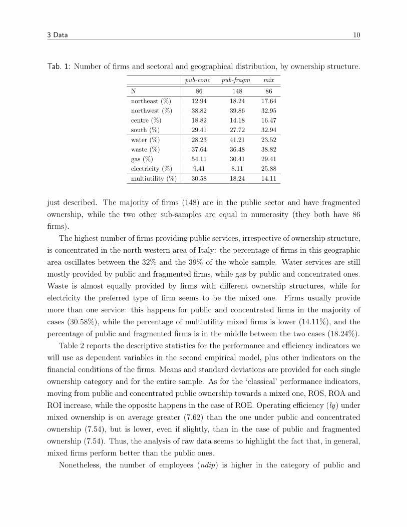
Tab. 1: Number of firms and sectoral and geographical distribution, by ownership structure.

pub-conc pub-fragm mix

N 86 148 86

northeast (%) 12.94 18.24 17.64

northwest (%) 38.82 39.86 32.95

centre (%) 18.82 14.18 16.47

south (%) 29.41 27.72 32.94

water (%) 28.23 41.21 23.52

waste (%) 37.64 36.48 38.82

gas (%) 54.11 30.41 29.41

electricity (%) 9.41 8.11 25.88

multiutility (%) 30.58 18.24 14.11

just described. The majority of firms (148) are in the public sector and have fragmented

ownership, while the two other sub-samples are equal in numerosity (they both have 86

firms).

The highest number of firms providing public services, irrespective of ownership structure,

is concentrated in the north-western area of Italy: the percentage of firms in this geographic

area oscillates between the 32% and the 39% of the whole sample. Water services are still

mostly provided by public and fragmented firms, while gas by public and concentrated ones.

Waste is almost equally provided by firms with different ownership structures, while for

electricity the preferred type of firm seems to be the mixed one. Firms usually provide

more than one service: this happens for public and concentrated firms in the majority of

cases (30.58%), while the percentage of multiutility mixed firms is lower (14.11%), and the

percentage of public and fragmented firms is in the middle between the two cases (18.24%).

Table 2 reports the descriptive statistics for the performance and efficiency indicators we

will use as dependent variables in the second empirical model, plus other indicators on the

financial conditions of the firms. Means and standard deviations are provided for each single

ownership category and for the entire sample. As for the ‘classical’ performance indicators,

moving from public and concentrated public ownership towards a mixed one, ROS, ROA and

ROI increase, while the opposite happens in the case of ROE. Operating efficiency (ly) under

mixed ownership is on average greater (7.62) than the one under public and concentrated

ownership (7.54), but is lower, even if slightly, than in the case of public and fragmented

ownership (7.54). Thus, the analysis of raw data seems to highlight the fact that, in general,

mixed firms perform better than the public ones.

Nonetheless, the number of employees (ndip) is higher in the category of public and

3 Data 11

Tab. 2: Firm descriptive statistics, total and by ownership category.

Own ROS ROA ROE ROI ly ndip ebitdasales

debtequity

totatt∗

pub- 2.13 1.29 8.32 4.28 7.54 183.33 7.27 2.51 42,682.38

conc (8.39) (24.76) (31.92) (9.89) (1.47) (952.71) (33.27) (17.27) (172,976.2)

pub- 2.87 2.01 7.21 4.71 7.64 84.61 11.27 3.53 29,270.88

fragm (8.43) (8.35) (26.61) (9.27) (1.49) (207.87) (23.61) (12.14) (78,215.58)

mix 3.23 4.04 7.05 6.66 7.62 108.48 14.28 1.99 63,723.21

(9.46) (10.27) (27.44) (9.85) (1.57) (342.71) (28.51) (9.72) (250,940.9)

total 2.78 2.42 7.45 5.19 7.61 116.79 11.13 2.79 42,901.38

(8.72) (14.88) (28.28) (9.64) (1.51) (534.55) (27.93) (12.99) (170,901.6)

Notes: N=321 firms. Standard deviations are in parentheses. ∗= values in thousands of euro.

concentrated (183), and lower for public and fragmented firms (84), while is in the middle

in case of mixed firms (108). This can be related to the fact that the number of employees

is both a sign of the size of the firm and excess employment: so public and concentrated

firms could be both big and with excess unemployment, while public and fragmented firms

are generally smaller in size.

Total assets (totatt), that can be used to represent the firm’s size, are higher for mixed

firms (63,723), are in the middle for public and concentrated firms (42,682) and the lowest

when ownership is fragmented (29,270). This, if compared with the data on the number of

employees, can indicate that mixed firms are bigger but with no excess employment with

respect to the public and concentrated firms.

Then, other indicators are provided: they also seem to highlight the fact that mixed

firms’ characteristics are better. Ebitda over sales (ebitda/sales), which is used to assess a

company’s profitability, increases shifting from public and concentrated ownership towards

mixed ownership. The debt-to-equity ratio (debt/equity), which indicates the proportion of

shareholders’ equity and debt used to finance a company’s assets, is higher with public and

fragmented firms (3.53), decreases with the concentration of firm (2.51), and is at its lowest

level (1.99) if the firm is mixed.

Finally, economic, financial and political indicators for the municipalities in the entire

sample and for the sub-sample for each macro area are provided in Table 3. Civic lists

(civica) are more diffused in the North-West, while left-wing mayor (L) are more diffused in

the Centre, and right-wing (R) in the South. Municipalities in north-western and central Italy

have higher taxing autonomy (autimpos). The level of extra-taxing autonomy (autextratrib)

is aligned in northern and central areas, while is lower in southern Italy.

The provincial unemployment rate (provunempl) is very high in the South (13.91), while

4 The empirical framework 12

it attains 5.85 in the Centre and a value around 4 in the North. Northern regions are

wealthier, especially in the West, where regional GDP (reggdp) attains 194,746, while the

Centre is in a middle-range position, with 66,938 of GDP and the South is very far away,

with the level of GDP at 48,395. Northeast and South of Italy are the areas with more

densely populated municipalities, with population density (pdensity) around 1,000 citizens

per squared-kilometer, while in the Centre and North-East local population is more dispersed

over the territory, since it attains 753 and 594 citizen per squared-kilometer, respectively.

Tab. 3: Economic, financial and political indicators for municipalities in the entire sample,and for the sub-sample for each macro area.

Northeast Northwest Centre South Total

civica 0.34 0.44 0.25 0.27 0.34

(0.48) (0.49) (0.43) (0.45) (0.47)

L 0.46 0.28 0.54 0.34 0.37

(0.49) (0.45) (0.49) (0.47) (0.48)

R 0.18 0.26 0.21 0.34 0.26

(0.39) (0.44) (0.41) (0.47) (0.43)

autextratrib 0.28 0.27 0.26 0.19 0.25

(0.12) (0.12) (0.13) (0.12) (0.12)

autimpos 0.43 0.51 0.48 0.38 0.45

(0.18) (0.16) (0.14) (0.15) (0.16)

provunempl 3.54 3.97 5.85 13.91 7.15

(0.94) (1.05) (2.09) (6.51) (5.79)

pdensity 594.34 1,031.18 753.09 983.29 899.17

(706.59) (1,392.27) (896.51) (1,897.97) (1,426.58)

reggdp 90,529.74 194,746 66,938.39 48,395.16 113,495.2

(38,346.36) (88,716.51) (43,082.6 ) (24,157.71) (88,665.9)

Notes: N=321 firms. Standard deviations are in parentheses. ∗= values in thousands of euro.

4 The empirical framework

The two different methods of analysis used to answer our questions are briefly reviewed in

the present Section.

The first research question concerns the determinants of the choice of ownership structure

in the year in which a new firm providing a local service is created. Given that the choice is

between more than two options and the dependent variable is composed by a set of categories

which cannot be ordered in a meaningful way, we will use a Multinomial Logit.

Then, we will study the effect of ownership structure on performance. However, in this


case there is a potential problem of endogeneity, if some unobservables affecting perfor-

mance also explain ownership structure. The endogenous nature of ownership structure and

its relation with performance has been stressed in literature (Palia, 2005; Boubakri et al.,

2005). Furthermore, in the present case the variable suffering from potential endogeneity is

polychotomous and unordered, requiring a special methodology to deal with the mentioned

problem. Thus, we use a relatively new method, developed by Bourguignon, Fournier and

Gurgand (2004), to correct the selection bias when it is specified as a Multinomial Logit.

Finally, given that in the model used to estimate performance and efficiency the outcome

equation depends upon the ownership regime, to retrieve the magnitude of these effects, we

will compute the Average Treatment on the Treated (ATT). The treatment effect measures the

impact of receiving a particular treatment (in this case, the choice of ownership structure),

upon a given outcome variable (i.e. performance and efficiency indicators). As we have

mentioned, the second question in the present study suffers from the problem of selection

bias, so the treated firms can differ from the non-treated for reasons that are different from

the treatment status per se. In the second model used, given its switching nature, the ATT

cannot be directly obtained from the coefficient of the treatment variable (own), as in a linear

Instrumental Variable model, and it will be computed with a procedure that is explained in

the last part of this Section.

4.1 The choice of ownership structure

In the first part of our analysis we try to find the determinants of the choice of ownership

structure through a Multinomial Logit model.

Suppose municipality i in the sample of N municipalities has to choose between 3 types

of ownership structures for the firm to be located in its area. If municipality i chooses the

ownership option j, it attains the level of expected social welfare Wij. In its social welfare

function, the municipality takes into account three components: the consumers’ net surplus

Si (generated by the service provided by the firm), the utility Ui of the manager running

the firm providing the service, and the shareholders’ expected dividends zi (which are partly

received by the municipality itself, proportionally to the shares it owns in the firm)10:

E [Wij] = E [f(Si, Ui, zi)] (1)

10 In principle, each of the elements on the right-hand side of the equation could vary also with j ; howeverwe omit it, since the data do not include choice-specific regressors.


We now redefine the model in terms of the choice that the municipality makes. It is clear

that the municipality i would choose the alternative that gives the highest social welfare,

which in turn is defined as a function of observable characteristics x′

i that are -as we have said-

related to the citizens’ conditions, and those of the firm and of the shareholders, and whose

impact changes across options (public and concentrated ownership, public and fragmented

ownership, mixed ownership), plus an additive error term εij:

Wij = βjx′

i + εij (2)

In this case we take into consideration only the data for the year in which the firm

has born, since the municipality bases its decision on ownership structure on its current

characteristics and those of the firm that is going to create. What is more, in our sample,

once the ownership structure has been chosen, it does not change over time.

Using a discrete variable owni, which takes value equal to 0, 1 or 2 if municipality i picks,

respectively, the alternative ownership structure public and concentrated (PC), public and

fragmented (PF ) or mixed (M), it follows that

P (owni = M) = P (WiM = max {WiPC , WiPF , WiM}) = P (βMx′

i + εiM > max βjx′

i + εij)

(3)

with j = PC, PF . This means that, even if we never observe the utility the municipality

associates with each ownership structure, we can infer from the choices it makes how it ranks

the possible outcomes. In equation (3) we show that mixed ownership (i.e. option M) is

chosen by the i-th municipality if, thanks to this alternative it attains the highest level of

social welfare.

Given that the coefficients are interpreted with respect to a reference ownership category11

(i.e. public and concentrated), we need a normalization of the parameters in order to restrict

the three probabilities to sum up to 1; thus, βPC = 0. Assuming that εij follows a log-

Weibull distribution (i.e. that the errors are mutually independent), the probabilities that a

municipality selects alternative PF or M are, respectively:

11 In the Multinomial Logit regression, one category of the response variable is chosen as a base (or ref-erence) outcome, so that it is omitted from the analysis: in the present case we will choose the first option(public and concentrated ownership). Thus, the obtained beta coefficients for the other two categories (pub-lic and fragmented and mixed ownership) represent the variation, associated with one unit change in thecorresponding regressor, of the odds ratios with respect to the reference category.


P (owni = PF ) =exp (βPF x′

i)

1 + exp (βPF x′

i) + exp (βMx′

i)(4)

P (owni = M) =exp (βMx′

i)

1 + exp (βPF x′

i) + exp (βMx′

i)(5)

Note that the first term in the denominator is 1: this is the logit normalization12 for the

base category, which in our model is public and concentrated ownership (i.e. option 1). This

option in turn has a probability to be selected that is equal to

P (owni = PC) =1

1 + exp (βPF x′

i) + exp (βMx′

i)(6)

The drawback of this model is the assumption that the error terms and, consequently,

the social welfare levels of any two alternatives are independent: the so-called property of

the independence of irrelevant alternatives (IIA)13.

Given that the first research question is “which are the determinants of the choice of

ownership structure made by the municipalities?”, the Multinomial Logit (MNL) model seems

convenient to our needs. We start from the idea that the municipality with the highest shares

in the new born firm is the one making the choice. Given its economic, financial and political

characteristics, the best suited form of public service delivery will be chosen.

Political variables (R, polalign) are needed since we want to test whether a conservative

party is more likely to set in place a mixed firm, and if this is even more likely when the

central government is right-wing as well.

Then, we want to test if the budgetary conditions of the local government do influence

its ownership choices, meaning that a municipality with lower financial autonomy chooses to

create a mixed firm in the hope of partly cutting monetary transfers with respect to a fully

public firm, but also trying to use this as a signal of commitment to a more tight financial

management: this will be done thanks to two indicators for the portion of revenues coming

from taxes and the portion of revenues extra-taxes (autimpos, autextratrib).

A series of variables controlling for the quantity of local services demand (cl1, cl2, cl3, cl5)

and the local economical conditions (in particular the economic development, dependency

12 The logistic function transforms the original range of [+∞;−∞] to one of [0; 1] .13 See McFadden (1974).


and unemployment, lgdpratio, ldepratio and lunempl) are are also included. It should be

pointed out that the latter variables are the (logarithm of) the ratio between the local and

the national indexes, in order to better capture the local conditions also with respect to the

national ones. The economies of scope (multiutility) and the industrial interest (waste, gas,

electricity) are considered, together with he geographical location (northeast, south, centre).

4.2 Selection bias corrections based on the Multinomial Logit

model

Once the municipality has chosen the preferred ownership option, the firm becomes operative,

producing at certain efficiency and profitability levels. To analyze the effects of ownership

structure on performance and efficiency, we will use a two-stage multinomial selection model.

This model is the Multinomial Logit equivalent of Heckman (1979) two-stage selection

model, where the identification strategy is based upon the choice of instrumental variables

and the presence of non-linearity of the selection stage. However, while in the Heckman

model there is only a choice between two options, and so there is only a correction term,

in this model there are as many correction terms as alternative choices14, as suggested by

Bourguignon et al. (2004).

As we said, the second part of the analysis will be dedicated to the study of the influence

of the chosen ownership (owni) and other firm characteristics (zi) on the various performance

and productivity indexes (yi) described in the previous section:

P (owni = j) =exp(x′

ijβj+µij)3

P

j=1

exp(x′

ijβj+µij)

yij = z′

ijδj +3∑

j=1

λ′

ijθj + µij + ξij

(7)

where λi represents the selection correction variable related to choice j. The parameter

θ is directly proportional to the correlation between the error terms in the performance

equation and the selection equation.

For this procedure, we use data covering the 2000-2008 period. Given that the treatment

14 In the MNL model corrected for selectivity bias the coefficients and the error terms for firms who receiveda different treatment are different. The model is an endogenous switching one, so we obtain a consistentestimate of the correction terms in the first step Multinomial Logit, and then we include them as additionalregressors in the corresponding equation. Finally, given that the performance equation has a continuousdependent variable, we run three linear regressions, corrected for the selectivity bias, on three sub-samplesin the second step.


variable (own) does not change over time, we will not use panel data methods, but we will

cluster the standard errors at firm level, since in the present case the only effect obtained

using panel models is to reduce the standard errors, but this will be obtained all the same

by using the data set as a pooled cross-section, using dummies to control for year-effects (µ)

and clustering firm-year observations.

The instruments used in the selection equation are: political variables (R, polalign);

public finance variables (autimpos, autextratrib); four out of the five the dummies (cl1, cl2,

cl3, cl4 ) for the dimensional class of the municipalities; sectoral and regional dummies. It

should be noted that most of them are the same we used to estimate the first model (i.e. the

determinants of the form of ownership). As we already explained in details in the previous

Section, we believe that the variables describing the demographic, financial and political

characteristics of the municipality are highly correlated with the ownership form, and at the

same time are not related to the firm performance.

The other variables added in the second-stage equation are the sectoral and regional

dummies. The sectoral variables are needed since the different sectors often imply different

performance (e.g. the electricity sector is usually more profitable than the waste sector);

the regional variables should capture both the traditional local services management (and,

consequently, performance) and economy of these macro-areas.

The variables lgdpratio and lunempl are added, and they are used to control for demo-

graphic and economic conditions.

4.3 The Average Treatment Effects on the Treated

The main focus of the second part of this analysis is to measure the difference in outcome

(i.e. performance and efficiency) for a given firm between receiving and non receiving the

treatment (i.e. mixed ownership).

However, since it is impossible to observe different treatments -and, consequently, different

outcomes- on the same firm (Holland, 1986) and the effect of treatment varies across firms, we

cannot infer the effect of the treatment: the problem is that we do not have the counterfactual

(i.e. an evidence on what would have happened to the firm if it would have not received this

treatment).

The objective here will be that of estimating the Average Treatment Effects on the Treated

(ATT), a well-known measure in the evaluation treatment literature (Heckman, Tobias, and

Vytlacil, 2001). It measures the average gain (in performance and efficiency) from a given

ownership choice for those who actually chose it. Thus, only those who decided ‘voluntarily’


to receive that treatment are considered, and the effect of this choice on the outcome of

individuals is computed through the ATT.

Given that in this case the evaluation is on multiple treatment, the identification of the

ATT would be implemented through pairwise correlation (Lechner, 2002). The ATT of

treatment k compared to treatment l is given by:

ATTkl = E[yk − yl | s = k] = E[yk | s = k] − E[yl | s = k] (8)

where E[yk | s = k] represents the performance for the firms in the ownership structure k (yk),

conditioning on the characteristics of firms that chose action k. The term E[yl | s = k] is the

performance for the firms in the ownership structure l (yl), conditioning on the characteristics

of firms that chose action k. In particular, since we are interested in the effect partial public

ownership has on firms’ performance and efficiency,with respect to a completely public one,

we estimate ATTM,PC and ATTM,PF :

ATTM,PC = E(yM |s = M) − E(yPC |s = M) (9)

ATTM,PF = E(yM |s = M) − E(yPF |s = M) (10)

In other words, the counterfactual question is: “What would have happened to those who

did receive treatment, if they had not received treatment?”. This means that the performance

indicator (the market outcome) of a mixed enterprise is compared to the performance the

same firm would have attained if it were not mixed (i.e. if it were public and with concentrated

or fragmented shares). Notice that the unconditional treatment effects are computed in the

sample of treated only.

The basic assumption is that firms with different characteristics self-select into one of the

three treatments on the basis of the observable and unobservable gains, so that unobservable

components of the outcomes affect the decision of individuals to participate. This means that

to estimate the ATT we should have not only the consistent estimates of the parameters in

the model, but also a measure of the bias. The unknown bias is obtained using the correction

terms and the probabilities from the selection-corrected MNL model. In the present case,

we will evaluate the choice of mixed ownership (s = M) against the choice of public and

concentrated ownership (s = PC) and against the choice of public and fragmented ownership

(s = PF ). It can be shown that the ATTs15 are given by:

15 Given that the same calculation applies to all municipalities, for simplicity we abstract from the sub-

5 Results and sensitivity analysis 19

ATTM,PC = (µM − µPC) − (δM − δPC) ∗ zj + (θM,M − θM,PC) ∗ λM,M +

+ (θPC,M − θPC,PC) ∗ λPC,M + (θPF,M − θPF,PC) ∗ λPF,M (11)

ATTM,PF = (µM − µPF ) − (δM − δPF ) ∗ zj + (θM,M − θM,PF ) ∗ λM,M +

+ (θPC,M − θPC,PF ) ∗ λPC,M + (θPF,M − θPF,PF ) ∗ λPF,M (12)

where all the λ terms are the selection correction variables connected to the different

choices, whose consistent estimate is obtained from first step Multinomial Logit. In particular,

λj,m represents the selectivity term for choice j, given the characteristics of municipalities who

chose option m.

The θ terms are the coefficients of the selection correction variables; θj,i = σjrj,i, where

σj is the the standard deviation of the error term in the first-step estimation for choice j, and

rj,i are the non-zero covariance parameter between the error term in the second and in the

first step estimation for choice j, given the characteristics of municipalities who chose option

m.

5 Results and sensitivity analysis

In this Section the main findings from our models are presented. In the first part we provide

the results for the determinants of the choice of ownership structure in the cross-section

containing the data on the year of firms’ birth only. The second part is devoted to the two-

step procedure that is used to find the relation between ownership and performance. The

third part of this Section describes the recovered ATTs.

5.1 The choice of ownership structure

In Table 4 we present the results for the determinants of the choice of ownership structure

(i.e. for the Multinomial Logit model): in this case the sample could be defined as a cross-

section, in the sense that we only consider the data related to the year of the firm’s birth

(annonascita).

Five different specifications are tested: we always control for the level of the economies

of scope (multiutility), and the variables for the local jurisdiction’s taxing (autimpos) and

extra-taxing (autextratrib) autonomy are always considered, since we are convinced that bud-

getary conditions are strictly related to the form of ownership chosen. Then we try different

indexes i.


specifications, adding and subtracting various political, regional, sectoral, demographic and

economic variables.

As expected, given that both autimpos and autextratrib have negative sign, the municipal-

ity’s budget autonomy has a negative effect on the choice of public and fragmented ownership,

and this effect is even more negative in case the choice is on the mixed structure: mixed firms

have a coefficient more than double with respect to public and fragmented firms for the first

variable, while it is at least 10% higher in case we consider the extra-taxing autonomy. The

inverse relation between ownership and autonomy entails that the more strict are the lo-

cal jurisdiction’s budgetary conditions, the more prone is the comune to choose the mixed

structure. Moreover, both autonomy indicators are always significant.

The fact that the mayor in power is conservative (R) pushes the choice of ownership

structure towards the public and concentrated one: at first sight, this could seem unexpected.

However, we should recall that in the last 20 years, the greatest moves towards privatization

and liberalization in Italy have been implemented by left-wing governments. Also note that

this political indicator is significant for all choices and specifications, except for the richest

one, in which appears insignificant for public and fragmented firms only. Furthermore, the

fact that the mayor’s ideology is aligned with that of the central government seems to have

a positive effect on the choice of mixed ownership, and a negative one in case of public and

fragmented ownership, even if it does not appear to be significant.

It should be pointed out that if a firm is a multiutility, the coefficient is in all cases highly

significant for mixed firms. The coefficient is negative, so mixed firms are more likely to serve

just one sector: this finding is coherent with what we deduced from the descriptive statistics.

In the richest specification, the number of inhabitants is positively and significantly related

with the choice of mixed ownership, and negatively related (or positively, but by a less extent)

with the choice of public and fragmented ownership, meaning that when the possibility of

economy of scale exploitation is available, mixed firms are preferred. Thus, we can infer that

mixed firms are more likely to exploit economies of scale than economies of scope.

In the southern area of Italy, the preferred form of ownership seems to be the public and

concentrated, and the same form of ownership seems to be preferred in case of high provincial

unemployment rate, which in turn is more likely in southern Italy. This evidence is in line

with the common knowledge about South Italy, and this could explain why coefficients are

significant only for the first of the two variables.

Finally, the preferred sector for mixed firms is electricity, while for public and fragmented

firms it seems to be water: it should be highlighted that electricity has been liberalized thanks

to the implementation of the European normative, starting from the European Directive


96/92/Ce, while the (very timid) attempt to liberalize water is quite recent. Moreover,

majors could have less incentives to provide water through a mixed firm due to the fact that

citizens -as proved by the recent Referendum results- usually believe it is a public good, to

be provided by the public sector.

We can conclude that the comune, in the year in which it has to choose the form of

ownership of the firm that will provide a given service to its community, will not only take

in consideration the number and the type of sectors served, but also the general economic

conditions (captured by the broad-area variables, plus the provincial unemployment rate and

the regional GDP). What is more, the hardness of the municipality budget constraints and

the political orientation seem highly determinant, confirming our theoretical predictions.


Tab. 4: Multinomial Logit for the choice of ownership structure.

(1) (2) (3) (4) (5)

pub-fragm mix pub-fragm mix pub-fragm mix pub-fragm mix pub-fragm mix

autimpos -0.884 -4.500*** -2.521** -5.265*** -2.328* -5.117*** -2.542** -5.059*** -2.472* -5.017***

(0.977) (1.103) (1.254) (1.500) (1.288) (1.559) (1.279) (1.509) (1.314) (1.568)

autextratrib -4.056*** -5.383*** -4.294*** -5.282*** -4.215*** -5.516*** -4.059*** -5.015*** -4.043*** -5.375***

(1.175) (1.293) (1.464) (1.784) (1.535) (1.891) (1.489) (1.798) (1.562) (1.908)

multiutility -0.455* -0.666** 0.165 -1.230** 0.128 -1.285** 0.253 -1.145** 0.227 -1.199**

(0.251) (0.328) (0.366) (0.527) (0.375) (0.529) (0.378) (0.528) (0.384) (0.530)

waste -0.984** 0.140 -0.959** 0.202 -1.073** 0.0842 -1.051** 0.140

(0.423) (0.524) (0.430) (0.530) (0.434) (0.533) (0.440) (0.538)

gas -1.254*** -0.281 -1.261*** -0.356 -1.447*** -0.396 -1.450*** -0.458

(0.417) (0.542) (0.423) (0.547) (0.434) (0.551) (0.439) (0.554)

electricity -0.534 1.753** -0.568 1.757** -0.712 1.663** -0.726 1.689**

(0.624) (0.728) (0.639) (0.734) (0.642) (0.737) (0.654) (0.744)

cl1 -0.455 0.287 -0.498 0.222 -0.608 0.00252 -0.629 -0.0387

(0.451) (0.541) (0.455) (0.544) (0.477) (0.560) (0.480) (0.563)

cl2 -0.719 -2.440** -0.702 -2.503** -0.922* -2.726** -0.900* -2.758**

(0.449) (1.120) (0.451) (1.123) (0.476) (1.127) (0.477) (1.127)

cl3 0.370 1.147** 0.347 1.103** 0.369 1.003* 0.373 0.983*

(0.438) (0.528) (0.440) (0.530) (0.455) (0.537) (0.456) (0.539)

cl5 -0.920* 0.968* -0.930* 0.937* -0.869 0.944 -0.887 0.904

(0.518) (0.565) (0.522) (0.569) (0.542) (0.577) (0.545) (0.579)

northeast 0.101 -0.0830 -0.167 -0.399 -0.0492 -0.215 -0.232 -0.444

(0.464) (0.577) (0.512) (0.628) (0.478) (0.586) (0.522) (0.633)

south -0.819* -0.960* -1.603* -1.222 -0.634 -0.784 -1.192 -0.837

(0.461) (0.562) (0.876) (0.981) (0.475) (0.575) (0.901) (1.000)

centre -0.329 -0.0985 -0.959 -0.508 -0.324 -0.0935 -0.714 -0.291

(0.438) (0.536) (0.633) (0.723) (0.456) (0.549) (0.659) (0.738)

lunempl 0.0989 -0.352 0.0690 -0.390

(0.432) (0.490) (0.445) (0.498)

lgdpratio -0.422 -0.408 -0.307 -0.299

(0.348) (0.366) (0.352) (0.368)

ldepratio 0.382 0.351 -0.491 -0.224

(3.393) (3.822) (3.443) (3.816)

R -0.952*** -0.915** -0.727* -1.024** -0.682 -0.935*

(0.315) (0.374) (0.440) (0.508) (0.446) (0.517)

polalign -0.402* 0.0837 -0.394 0.0988

(0.239) (0.279) (0.241) (0.281)

constant 2.517*** 3.858*** 4.417*** 3.806*** -0.466 -1.188 5.105*** 4.037*** -1.976 -1.904

(0.726) (0.759) (1.114) (1.300) (19.13) (21.06) (1.154) (1.341) (19.29) (20.87)

N. of obs. 312 312 312 312 312 312 312 312 312 312

Pseudo R2 0.078 0.078 0.168 0.168 0.182 0.182 0.194 0.194 0.203 0.203

Dependent variable is ownership choice (own). Standard errors in parentheses. *** p<0.01, ** p<0.05, * p<0.1.


5.2 Performance and efficiency in local services providers

We now turn to the effects ownership structure has on the performance and efficiency of

these firms, using the Multinomial Logit corrections for selectivity bias. Table 5 presents the

results from the first-step estimates of the model. Given that the municipality’s dimensional

class (cl1, cl2, cl3 and cl4 ), its political alignment (R, polalign) and its budgetary conditions

(autimpos, autextratrib) are used as instruments in the second step of the model, it is it

worthy to underline that they frequently appear to be significant, especially for the choice

of mixed ownership. Note that all the variables included were also included in the previous

model: the more similar is specification (4).

As most of the coefficients and their sign are aligned with the previous findings, we will

only briefly comment the results. In particular, the political orientation and the taxing

autonomy are significant for both types of firms, while the dimensional class is significant

only for cl2 and cl3, for mixed and public and fragmented firms, respectively. As for the

other variables, their sign is aligned with those obtained in Table 4, when we were studying

the determinants of the choice of ownership structure in the year of the utility’s formation.


Tab. 5: The Multinomial Logit in the first step of estimation.

pub-fragm mix

Coefficient Standard Error Coefficient Standard Error

R -0.949*** (0.267) -0.768** (0.334)

polalign -0.043 (0.039) -0.004 (0.046)

autimpos -2.395* (1.257) -3.100** (1.465)

autextratrib -2.860** (1.287) -1.870 (1.436)

multiutility 0.251 (0.364) -1.158** (0.528)

nascita 0.092 (0.098) 0.483*** (0.136)

cl1 0.137 (0.571) -0.631 (0.621)

cl2 -0.231 (0.525) -2.494*** (0.772)

cl3 1.040** (0.526) -0.225 (0.599)

cl4 0.820 (0.508) -0.958 (0.608)

waste -0.890** (0.425) 0.191 (0.578)

electricity -0.711 (0.701) 1.697** (0.817)

gas -1.522*** (0.404) -0.694 (0.550)

northeast 0.043 (0.476) 0.072 (0.548)

south -0.650 (0.408) -0.628 (0.510)

centre -0.330 (0.440) -0.163 (0.514)

constant 3.012*** (1.139) 0.395 (1.348)

year dummies yes yes

N. of obs. 2,825 2,825

Pseudo R2 0.189 0.189

Robust standard errors in parentheses. *** p<0.01, ** p<0.05, * p<0.1.

5.2.1 Second step estimation with selection corrected outcomes

In this second step of the second model, three different correction coefficients (λ1, λ2, λ3),

one for each ownership choice, are computed in the first step and are used to eliminate the

selection bias. Recall that we do not use the longitudinal dimension of the data, since the

invariance of the treatment variable (own) over time would not bring additional information

to our estimation. As a matter of fact, we exploit the abundance of firm data clustering

observations at firm-level, and obtaining robust standard errors.

Tables 6-11 show the results of the second stage equation for each efficiency and perfor-

mance indicator for the three ownership categories and compare them with Ordinary Least

Squares results: Return on Sales (Table 6), Return on Assets (Table 7), Return on Equity

(Table 8), Return on Investments (Table 9), employment (Table 10), and technical efficiency


(Table 11). Notice that the model used in this Section is an endogenous switching model;

thus, the lambda’s coefficients are not the ATTs, which will be retrieved in the next Section.

Thus, now we will just highlight the variables which are more significant in determining the

outcomes, and the direction of their contribution.

In case of public and concentrated ownership, the more significant coefficients in determin-

ing performance and efficiency are the geographical location and the local economic conditions

(the logarithm of the ratio between regional and national GDP and between provincial and

national unemployment rate). In general, the most inefficient public and concentrated firms

are in the North-West area of Italy, given that our indicators in all other areas are positive

in sign: this is somehow unexpected. However, given that most of the mixed firms are con-

centrated in North-West, we can think that the firms with public and concentrated firms are

those which would be the most inefficient. The gap of unemployment at provincial level with

respect to the national one (lunempl), has -as one would expect, since big public firms tend

to keep excess employment- a positive effect on the number of employees in the firm, while

it negatively affects all the performance indicators, and the coefficients are significant in the

majority of cases. As for the ratio between regional and national economic development

(lgdpratio), from the positive sign of the coefficient for most of the indicators we can infer

that a relative improvement in the regional economic conditions (i.e. regional development)

increases occupation, efficiency and performance. Sectors have a significant effect only in

determining ROE and productive efficiency, and the fact of serving more than on sector has

a (negative) significant effect only on productive efficiency.

When we turn to public and fragmented firms, the fact that a firm serves more than

one sector has a positive effect on the number of employees and on performance, and it

shows a negative effect for productive efficiency (ly). Multiutility has a negative effect on

all indicators, while firms serving the energy sector (gas and electricity) show a decreasing

number of employees and a positive effect on productive efficiency, and this effect is significant.

It is indeed well known that the sectors of electricity and gas are the most liberalized, and

also the most profitable sectors among utilities. Size has a positive and significant effect for

ROS and ROA only, indicating the the greater contribution of economies of scale to their

increase. Quite predictably, unemployment has a negative effect on all our indicators, except

with the number of employees with which it is positively related. We find that all regional

coefficients are positive for the performance indicators; once again, these coefficients report

the relative effect with respect to the north-western macro area, and it could be a sign that

in that area the most inefficient firms are generally those under public ownership, while in


other areas, as the South of Italy, public ownership is nearly always the preferred choice.

Finally, we turn to the performance and efficiency indicators for the firms that chose the

mixed structure. Note that now the sign of many coefficients is reversed with respect to the

previous cases. Firms serving in more than one sector have better and significant results than

those operating in one sector (except for efficiency and ROE): mixed firms are more able to

exploit economies of scope. Firms operating in regions which are different from northwest

perform generally worst and have a higher number of employees. Quite unexpected is the

effect of ‘experience’ of the firm: while for public and concentrated firms the direction of the

effect was not clear-cut, with low and insignificant coefficients, it now turns negative and

significant for ROS, ROA and ROE: this could explain why, after 2000, the number of mixed

firms born has decreased dramatically. It is possible that mixed firms are more susceptible

to the outside conditions with respect to their public counterparts.


Tab. 6: ROS Ordinary Least Squares and selection correction (using the the Dubin and Mc-Fadden method with the correction suggested by Bourguignon et al. (2004)) esti-mates.

OLS Selmlogall pub-fragm pub-conc mix

nascita -0.035 0.705** -0.387 -1.429***(0.161) (0.301) (0.444) (0.503)

size 0.691*** 0.787*** -0.106 1.111***(0.130) (0.195) (0.323) (0.285)

multiutility -0.815 -3.451*** 0.571 5.006**(0.584) (1.167) (1.408) (1.949)

waste -0.607 2.642** -2.583 -2.415(0.614) (1.146) (1.623) (1.504)

electricity 1.695* 6.811*** -3.398 -5.580*(0.874) (1.765) (2.587) (2.981)

gas 1.331** 5.002*** 0.464 -3.282**(0.634) (1.447) (1.863) (1.669)

lgdpratio -0.148 0.307 3.586** -0.082(0.415) (0.607) (1.469) (0.655)

ldepratio 6.917 16.08* 13.64 -0.024(5.776) (8.871) (19.61) (8.536)

lunempl -3.395*** -6.052*** -2.552 -3.370***(0.771) (1.416) (1.992) (1.069)

northeast 0.355 0.073 7.502*** -3.206(0.781) (1.038) (1.902) (2.054)

south 3.227** 8.727*** 10.02*** -1.223(1.251) (2.265) (3.756) (1.706)

centre 2.115** 3.927** 7.797*** -0.728(0.859) (1.647) (2.178) (1.604)

λ0 27.57*** -6.371* 15.70*(10.01) (3.511) (9.003)

λ1 12.79** -12.69* 14.38**(5.638) (7.307) (6.615)

λ2 31.26*** -17.92** 0.158(9.736) (8.110) (3.294)

constant 14.06 55.83 124.8 0.847(30.76) (45.99) (108.9) (46.03)

N. of obs. 1,406 634 361 388R2 0.069 0.142 0.101 0.186Bootstrapped (200 repetitions) standard errors in parenthesis; observations clustered at the firm level.

Year dummies included. *** p<0.01, ** p<0.05, * p<0.1.


Tab. 7: ROA Ordinary Least Squares and selection correction (using the the Dubin andMcFadden method with the correction suggested by Bourguignon et al. (2004))estimates.


nascita 0.130 0.195 2.169 -1.315***(0.265) (0.245) (1.788) (0.432)

size 0.300 0.012 2.169 0.038(0.213) (0.167) (1.971) (0.339)

multiutility -2.737*** -2.721** -7.777 0.624(0.969) (1.328) (5.338) (1.315)

waste 0.263 2.508** 2.825 -3.912***(1.029) (1.186) (3.768) (1.232)

electricity 4.922*** 2.846 12.66 1.594(1.364) (1.937) (9.741) (2.056)

gas 1.476 3.790*** 3.112 -3.617***(1.058) (1.406) (3.893) (1.375)

lgdpratio -1.688*** 0.164 -3.126 -0.566(0.596) (0.654) (5.480) (0.999)

ldepratio -16.11* 13.28 -123.8 10.75(8.862) (12.58) (103.9) (8.968)

lunempl -4.766*** -3.048* -16.93 -3.872***(1.274) (1.767) (12.83) (0.990)

northeast -2.759** 1.038 -2.524 -5.882***(1.236) (0.963) (5.848) (1.818)

south -0.719 2.096 11.93 -0.385(1.974) (2.021) (7.456) (1.958)

centre 1.160 2.122 16.26* -2.655**(1.395) (1.508) (8.374) (1.286)

λ0 9.710 -22.11 6.880(8.383) (15.33) (8.394)

λ1 5.842 -57.72* 9.919(4.315) (32.54) (7.709)

λ2 13.06 -10.66 -1.705(8.825) (21.08) (3.428)

constant -107.6** 59.15 -664.8 57.83(45.93) (67.51) (584.0) (52.03)

N.of obs. 1,511 668 382 435R2 0.056 0.064 0.154 0.270Bootstrapped (200 repetitions) standard errors in parenthesis; observations clustered at the firm level.



Tab. 8: ROE Ordinary Least Squares and selection correction (using the the Dubin andMcFadden method with the correction suggested by Bourguignon et al. (2004))estimates.


nascita -0.991* -0.940 -1.364 -2.926**(0.508) (1.033) (1.613) (1.192)

size 0.152 0.328 0.531 0.965(0.409) (0.583) (1.011) (0.669)

multiutility -8.603*** -5.698* -9.516** -3.602(1.864) (3.343) (4.047) (4.424)

waste 1.909 2.594 7.963 -8.348**(1.983) (3.352) (6.704) (4.109)

electricity 11.59*** 4.566 19.85*** 2.895(2.603) (6.812) (7.037) (6.436)

gas 9.452*** 13.67*** 16.74** -1.333(2.035) (4.490) (7.625) (5.145)

lgdpratio 0.332 4.122** 7.323* 0.292(1.151) (1.921) (3.747) (1.629)

ldepratio 25.11 44.85 30.62 29.46(17.10) (32.62) (56.81) (26.49)

lunempl -8.808*** -3.682 -21.44*** -12.71***(2.462) (3.731) (7.739) (3.141)

northeast -3.714 5.494 4.194 -19.26***(2.369) (3.730) (5.224) (4.009)

south 6.317* 8.261 40.02*** 3.404(3.813) (5.922) (14.57) (5.927)

centre 3.485 1.563 29.50** -2.794(2.674) (4.320) (11.59) (4.077)

λ0 -13.01 -21.03* 12.81(28.74) (12.19) (26.32)

λ1 -3.555 -70.38*** 11.49(17.75) (24.84) (21.19)

λ2 -8.511 -35.58 -3.816(29.03) (28.38) (9.794)

constant 112.2 256.0 209.1 155.4(88.70) (169.9) (277.3) (131.6)




Tab. 9: ROI Ordinary Least Squares and selection correction (using the the Dubin and Mc-Fadden method with the correction suggested by Bourguignon et al. (2004)) esti-mates.


nascita 0.457** 0.822* 0.069 -0.593(0.205) (0.423) (0.423) (0.526)

size -0.148 -0.141 -0.562 0.172(0.172) (0.306) (0.552) (0.300)

multiutility -0.580 -1.422 0.573 2.206(0.787) (1.480) (2.141) (2.044)

waste 2.394*** 4.867*** 2.836 -2.032(0.834) (1.590) (2.543) (1.946)

electricity 0.779 4.259 -3.781 -1.731(1.072) (2.975) (3.029) (2.323)

gas -0.827 1.231 4.534 -7.087***(0.869) (1.854) (3.147) (2.142)

lgdpratio 0.675 2.336** 3.708* 1.082(0.510) (0.937) (2.129) (0.990)

ldepratio 29.13*** 52.59*** 29.61 33.25**(8.027) (16.49) (27.93) (13.27)

lunempl -3.099*** -0.438 -5.394 -5.769***(1.198) (1.986) (3.707) (2.215)

northeast 0.085 2.530 4.648* -3.394*(0.960) (1.580) (2.453) (1.928)

south 6.081*** 5.453** 20.73*** 7.935**(1.781) (2.622) (6.947) (3.305)

centre 3.272*** 3.787** 12.08** 1.134(1.172) (1.694) (5.605) (1.970)

λ0 0.689 -0.858 -7.094(9.532) (7.223) (10.47)

λ1 -0.0329 -13.98 -2.859(5.515) (16.29) (7.684)

λ2 8.759 -5.366 -6.378*(9.817) (17.49) (3.611)

constant 151.0*** 279.3*** 186.3 178.1**(42.20) (87.16) (144.6) (73.32)

N. of obs. 932 432 214 272R2 0.062 0.112 0.168 0.162Bootstrapped (200 repetitions) standard errors in parenthesis; observations clustered at the firm level.



Tab. 10: OCC Ordinary Least Squares and selection correction (using the the Dubin andMcFadden method with the correction suggested by Bourguignon et al. (2004))estimates.


nascita 0.015 -0.351*** -0.172 -0.217(0.025) (0.131) (0.125) (0.142)

size 0.553*** 0.441*** 0.494*** 0.602***(0.020) (0.045) (0.064 (0.048)

multiutility 0.670*** 2.116*** 1.173*** 1.235***(0.088) (0.450) (0.386) (0.422)

waste 0.644*** 0.041 -0.401 0.462(0.093) (0.347) (0.321) (0.304)

electricity -0.529*** -3.066*** -2.119*** -1.245*(0.138) (0.828) (0.776) (0.676)

gas -1.036*** -1.391*** -2.145*** -0.870***(0.101) (0.374) (0.393) (0.328)

lgdpratio -0.172*** 0.043 -0.348** -0.253***(0.055) (0.098) (0.171) (0.096)

lunempl 0.569*** 0.455** 0.728** 0.194(0.117) (0.232) (0.333) (0.193)

northeast 0.390*** 0.639*** 0.820** -0.135(0.120) (0.222) (0.337) (0.249)

south -0.223 -0.518 -0.405 0.388(0.183) (0.339) (0.615) (0.273)

centre 0.339*** 0.140 -0.024 0.391(0.131) (0.255) (0.428) (0.297)

λ0 -0.282 -0.434 -0.740(2.439) (0.794) (1.724)

λ1 0.601 3.907 -2.302(1.390) (2.411) (1.574)

λ2 -5.215 -2.207 -2.112**(3.184) (2.825) (0.823)

constant -9.424*** -2.769 -8.422** -10.10***(1.050) (2.046) (3.312) (2.867)




Tab. 11: LY Ordinary Least Squares and selection correction (using the the Dubin and Mc-Fadden method with the correction suggested by Bourguignon et al. (2004)) esti-mates.


nascita -0.017 0.138 0.062 0.158(0.024) (0.114) (0.105) (0.116)

size 0.255*** 0.331*** 0.328*** 0.226***(0.019) (0.041) (0.064) (0.044)

multiutility -1.109*** -1.633*** -1.362*** -1.403***(0.083) (0.383) (0.366) (0.391)

waste 0.125 0.196 0.852** 0.009(0.089) (0.279) (0.376) (0.260)

electricity 0.658*** 1.557** 2.021*** 0.875(0.130) (0.717) (0.730) (0.641)

gas 1.614*** 1.290*** 2.215*** 1.666***(0.095) (0.297) (0.447) (0.357)

lgdpratio 0.181*** 0.001 0.259 0.283***(0.052) (0.088) (0.167) (0.095)

lunempl -0.762*** -0.507** -1.144*** -0.740***(0.112) (0.205) (0.292) (0.164)

northeast -0.277** -0.255 -0.377 -0.175(0.114) (0.177) (0.369) (0.232)

south 0.247 0.087 0.965* -0.116(0.174) (0.297) (0.570) (0.262)

centre 0.0814 -0.311 0.706* 0.162(0.124) (0.219) (0.391) (0.280)

λ0 -6.820*** -0.825 2.514*(2.509) (0.770) (1.390)

λ1 -2.921* -5.669*** 1.821(1.555) (1.993) (1.487)

λ2 -2.977 -1.131 1.927***(3.152) (2.512) (0.654)

constant 5.785*** -0.713 1.663 7.954***(1.061) (1.762) (3.429) (2.738)


Year dummies included.*** p<0.01, ** p<0.05, * p<0.1.


During our estimation we subjected our instruments to a series of informal tests (due to

the lack of formal tests in this setting). First of all, we test jointly our instruments after

the multinomial treatment equation and find that they are relevant. The F-test results yield

a Chi-squared statistics of 349.18, which satisfies the Stock and Yogo (2005) rule of thumb

value for the strength of instruments.

Then, we need to check the validity of instruments (i.e. that they are not correlated with

the error term in the second step equation). This assumption can be tested, since we have an

overidentified model (i.e. the number of instrumental variables is greater then the number of

variables suffering from endogeneity), so we have enough information to carry out the Sargan

test. We perform this test by multiplying the number of observations (N) and the R2 of an

auxiliary linear regression of selmlog residuals upon the all instruments (Verbeek, 2004).

When the null of this test is rejected16, this means that the sample evidence is consistent

with the exogeneity of instruments. Results for this tests are shown in Table 12.

Tab. 12: Sargan test results.

ROS ROA ROE ROI occ LY

pub-fragm NR2 19.937 30.244 11.149 13.354 43.256 15.197

p-value 0.174 0.011 0.742 0.575 >0.001 0.437

pub-conc NR2 8.312 10.945 7.082 3.649 12.678 13.760

p-value 0.911 0.756 0.955 0.999 0.627 0.543

mix NR2 19.066 4.926 7.769 3.717 24.622 21.690

p-value 0.211 0.993 0.933 0.998 0.055 0.116

χ2 24.996

5.3 The ATT for mixed firms

As we mentioned above, the ATT answers to the question ‘what would have happened to

those who did receive treatment, if they had not received treatment?’. In this case we take

into consideration various indexes of performance and efficiency, and we check whether the

choice of mixed ownership has a positive effect or not.

First of all, let us consider the canonical performance indicators.

Mixed firms have worst ROS than the public and concentrated firms, since if mixed

firms would have been public and concentrated they would have had a positive and highly

16 When the p-value is higher than 0.05.


significant effect on their ROS (72,338), but the effect is halved when when we consider what

would have happened if ownership would have been public and fragmented (36,445). As this

indicator measures operating efficiency, since it provides information on how much profit is

being produced per euro of sales, we can conclude that -on average- mixed firms are way

worst than public and concentrated but worst than public and fragmented.

When taking into consideration ROA, given that this indicator could give an idea on how

efficient the firm is in using its assets to generate earnings, we can conclude that this is done

better -with respect to a mixed firm- by a public and concentrated firm (since with this kind

of ownership structure the ROA would increase by 75,029) and by a public and fragmented

firm, even if by a much lower extent (given that the effect would be of 6,406).

ROE measures how much profit a firm generates with the money shareholders have in-

vested: given that the sign of the ATT is positive in the first case and negative in the

second, mixed firms are in the middle from this point of view. What is more, public and

fragmented firms have a coefficient which is two times bigger (41,284) than the one for public

and concentrated firms (-29,427), so that we can conclude that public and concentrated firms

badly repay their shareholders. In general, the negative coefficients in this case represent the

fact that mixed firms are more remunerative for shareholders than public concentrated ones,

partly justifying the fact that municipal ownership in mixed firms has been called ‘municipal

capitalism’.

When looking at the efficiency of investments, we see that ROI is much better both in

case of public and concentrated (21,436) and public and fragmented enterprises (13,095).

If we only consider these classic performance indicators, we would have to conclude that

mixed ownership does not improve the firm performance.

We now turn to the efficiency indicators of the firms, referring to the employment and

productive efficiency levels.

Given that the first coefficient is -29,839, the logarithm of the number of workers (occ)

would decrease if the mixed firm would be public and fragmented, while it would decrease by a

lower extent (-17,061) in case of public and concentrated firms. This means that if the mixed

firm would have been public, the number of employees would be lower. The difference in the

magnitude of the effect could be due to the fact that the first type of public firm serves a high

number of municipalities, often dispersed in the territory, while the latter serves just one or

very few municipalities, and it could also exploit the economies of scale due to its dimension.

Even if one would think that mixed ownership would mean less excess employment (Shleifer

and Vishny, 1994), it is also true that the public shareholder is still present in the firm, so

6 Summary and Conclusions 35

that he can still try to purse his own objectives.

Finally, productive efficiency (ly) would be much better with mixed ownership in both

cases; in particular, changing the ownership structure would entail a loss in technical efficiency

of -2.711, while the loss would be higher (-6.668) if the change would be towards public and

concentrated ownership. This last point seems to confirm the theory that a mixed firm could

balance the advantages of private and public firms (Eckel and Vining, 1985; Marra, 2006;

Boggio, 2010), increasing the incentives for the firm’s manager to exert effort and ameliorate

the firm’s productive efficiency.

Tab. 13: Average Treatment Effects (ATT).

ATTM,PF ATTM,PC

Indexes coeff. St. Err. N coeff. St. Err. N

ROS 72.338∗ 1.966 435 36.445∗ 1.935 431

ROA 75.029∗ 1.155 435 6.406∗ 0.893 431

ROE 41.284∗ 0.785 435 -29.427∗ 0.596 431

ROI 21.436∗ 0.669 435 13.095∗ 0.590 431

occ -23.839∗ 0.289 754 -17.161∗ 0.279 754

ly -2.711∗ 0.201 754 -6.668∗ 0.206 754

*** p<0.01, ** p<0.05, * p<0.1.

6 Summary and Conclusions

In this paper we have tried to find the reasons that push a municipality to form a firm with a

given ownership structure, since it faces a number of alternatives (public and concentrated,

public and fragmented, mixed). Then, we also tried to assess which are the consequences of

the choice of a given ownership category for a series of performance and efficiency indicators.

To explore this problem we have used a unique data set, formed through the combination of

various sources.

We have found that not only the municipal sectoral interest is important in the choice

of ownership, but also political variables. Moreover, the local government’s budgetary con-

straints appear always a very important element affecting this choice. However, while more

mixed firms have been formed at the beginning of the century, the enthusiasm for this alter-

native method of provision has progressively worn off.

This could be due to the fact that, taking into consideration the classical performance

indicators, mixed firms appear very often to perform poorly with respect to the two forms of

public provision. This underlines the fact that privatizing the utilities sector ‘as it is’ would


have little sense if this is not accompanied by a dramatic reduction in the level of subsidies

and if the level of liberalization in the system is not increased. However, technical efficiency

seems higher, indicating that the fact that private and public shareholders coexist in the

firm, and that the public shareholder is a regulator as well, could provide better incentives

for the firm.

References

[1] Biais, B., and E. Perotti, (2002). ‘Machiavellian Privatization’. American Economic

Review, 92(1):240–258.

[2] Bianchi, P., B. Bortolotti, L. Pellizzola, and C. Scarpa, (2009). Comuni S.p.A. : il

capitalismo municipale in Italia, Il Mulino.

[3] Boardman, A., and A.R. Vining, (1989). ‘Ownership and Performance in Competitive

Enviroments: a Comparison of the Performance of Private, Mixed, and State-Owned

Enterprises’. Journal of Law & Economics, 32:1-33.

[4] Boggio, M., (2010). Municipal Capitalism, Regulatory Federalism and Politics. Unpub-

lished.

[5] Bortolotti, B., and M. Faccio, (2008). ‘Government Control of Privatized Firms’, Review

of Financial Studies, 1:1-33.

[6] Bortolotti, B., M. Fantini, and D. Siniscalco, (2003). ‘Privatisation around the World:

Evidence from Panel Data’. Journal of Public Economics, 88:305-332.

[7] Boubakri, N., J. Cosset, and O. Guedhami, (2005). ‘Post-Privatization Corporate Gov-

ernance: the Role of Ownership Structure in Investor Protection’. Journal of Financial

Economics, 76(2):369-399.

[8] Boubakri, N., J. Cosset, and O. Guedhami, (2009). ‘From State to Private Ownership:

Issues from Strategic Industries’. Journal of Banking and Finance, 33(2):367-379.

[9] Bourguignon, F., M. Fournier, and M. Gurgand, (2004). ‘Selection Bias Corrections

Based on the Multinomial Logit Model: Monte-Carlo Comparisons’. DELTA Working

Papers n. 2004-20.


[10] Branco, F., and A. Mello, (1991). ‘A Theory of Partial Sales and Underpricing in Pri-

vatization’. MIT, mimeo.

[11] CEEP, (2010). Mapping the Public Services. Technical report.

[12] Dubin, J. A., and D. L. McFadden, (1984). ‘An Econometric Analysis of Residential

Electric Appliance Holdings and Consumption’. Econometrica, 52(2):345-62.

[13] Eckel, C., and A. Vining, (1985). ‘Elements of a Theory of Mixed Enterprise’. Scottish

Journal of Political Economy, 32(1):82-94.

[14] Heckman, J., (1979). ‘Sample Selection Bias as a Specification Error’. Econometrica,

47(1):153-61.

[15] Heckman, J., J. L. Tobias, and E. Vytlacil, (2001). ‘Four Parameters of Interest in the

Evaluation of Social Programs’, Southern Economic Journal, 68(2):210-223.

[16] Holland, P. W., (1986). ‘Statistics and Causal Inference’. Journal of the American Sta-

tistical Association, 81(396):945-960.

[17] La Porta, R., F. Lopez-de-Silanes, A. Shleifer, and R. W. Vishny, (1999). ‘The Quality

of Government’. Journal of Law, Economics, and Organization, 15:222-279.

[18] Lechner, M., (2002). ‘Some Practical Issues in the Evaluation of Heterogeneous Labour.

Market Programmes by Matching Methods’. Journal of the Royal Statistical Society,

165:59-82.

[19] Marra, A., (2006). ‘Mixed Public-Private Enterprises in Europe: Economic Theory and

an Empirical Analysis of Italian Water Utilities,’ Bruges European Economic Research

Papers n.4.

[20] McFadden, D. L., (1974). ‘The Measurement of Urban Travel Demand’. Journal of Public

Economics, 3(4):303-328.

[21] Palia, D., (2001). ‘The Endogeneity of Managerial Compensation in Firm Valuation:a

Solution’. Review of Financial Studies 14:735-764.

[22] Perotti, E., (1995). ‘Credible Privatization’. American Economic Review, 85(4):847-859.

[23] Roland, G., (2000). Transition and Economics. MIT Press, Cambridge, MA.


[24] Shleifer, A., and R. W. Vishny, (1994). ‘Politicians and Firms’. The Quarterly Journal

of Economics, 109(4):995-1025.

[25] Stock, J. H., and M. Yogo, (2005). ‘Testing for Weak Instruments in Linear IV Re-

gression’. In Identification and Inference for Econometric Models: Essays in Honor of

Thomas Rothenberg, ed. Andrews and Stock, pp. 80-108, Cambridge University Press.

[26] Verbeek, M., (2004). A Guide to Modern Econometrics, Wiley.

[27] Vickers, J., and G. Yarrow, (1991). ‘Economics Perspectives on Privatization’. Journal

of Economic Perspectives, 5(2):111-132.

municipal capitalism: from state to mixed ownership in local public

Documents