music: a time-frequency approach - university of … · 2009-01-03 · music: a time-frequency...

$: Music: A time-frequency approach - University of … · 2009-01-03 · Music: A time-frequency approach Gary W. Don Department of Music and Theatre Arts ... fractal music are analysed$
Music: A time-frequency approach

Gary W. Don

Department of Music and Theatre Arts

University of Wisconsin–Eau Claire

Eau Claire, WI 54702–4004

E-mail: [email protected], Tel. 715-836-4216, Fax. 715-836-3952

James S. Walker∗

Department of Mathematics

University of Wisconsin–Eau Claire

Eau Claire, WI 54702–4004

E-mail: [email protected], Tel. 715-836-4835, Fax. 715-836-2924

(Received 00 Month 200x; In final form 00 Month 200x )

∗Corresponding author

1

2 Music: A time-frequency approach

Gabor transforms and scalograms are used for mathematically analysing music, identifying patterns in the time-frequency structure ofmusic at multiple time scales, and providing insight into the nature of music. Passages from classical music, popular song, bird song, andfractal music are analysed using a synthesis of the generative theory of tonal music and the mathematical methods of Gabor transformsand scalograms. Applications to musical processing, and musical synthesis are described using inversion of Gabor transforms.

Keywords: music theory, musical analysis, music processing, time-frequency analysis, Gabor transforms, spectrogramsAMS 2000 Subject Classification Codes: 42A99, 00A06, 00A69

The relation between mathematics and music has a long and rich history, including: Pythagorean harmonic

theory, fundamentals and overtones, and frequency and pitch (see e.g. [2]). In this article, we describe an

approach to music that is a synthesis of ideas from musical theory and techniques of spectral analysis. The

ideas from musical theory are the generative theory of tonal music created by Jackendoff and Lerdahl; while

the techniques of spectral analysis include Gabor transforms and scalograms. We hope this interdisciplinary

work will shed some light on the nature of music and its connection with mathematics.

The paper has three sections. In Section 1, we summarize the mathematical theory of Gabor transforms

and scalograms. We apply Gabor transforms and scalograms in Section 2, where we analyse four musical

passages: (1) the famous ending passage of Stravinsky’s Firebird Suite; (2) a passage of the song, Buenos

Aires, from the popular musical Evita; (3) a warbler’s song; and (4) a fractal musical passage based on

Sierpinski’s triangle. These analyses will show that Gabor transforms and scalograms provide powerful

objective tools for performing the type of multi-timescale analysis of music described by Jackendoff and

Lerdahl. We also contribute some multi-timescale analysis of rhythmic aspects of music that are not

readily accessible using traditional tools of rhythmic analysis. The interaction between rhythm, voice, and

instrumental tones in the Buenos Aires passage, for instance, is a fine example of the rich territory that a

wide variety of music provides for spectral analysis. Section 3 describes four applications to music processing

and synthesis: (1) removing noise from a recording; (2) amplifying a selected instrumental passage while

preserving background accompaniment; (3) changing the timing and emphasis of piano playing with an

orchestra; and (4) creating new sounds.

1 Gabor transforms and scalograms

Our tools for analysing music are Gabor transforms and scalograms [13–15, 18]. Gabor transforms have

been widely employed for over half a century in linguistics and in the study of bird song (where they are

also known as spectrograms or sonograms), and heavily used in speech recognition and communication

theory (where they are also known as short-time Fourier transforms). They deserve to be better known

in the mathematical world as they are as least as useful as the well-known Fourier series. Here we will

show how they provide a powerful tool for analysing and synthesizing music. Scalograms represent a more

recent approach to music based on wavelet analysis. They provide an important complement to our basic

tool of Gabor transforms.

We assume that readers are familiar with the basic notions of Fourier analysis and musical tones: that a

note from a musical instrument can be expressed as a linear combination of sinusoidals whose frequencies

are all integral multiples of a fundamental (the fundamental and its overtones), and that the coefficients

of this linear combination (amplitudes of the sinusoidals) are the Fourier coefficients. Of course, in our

Gary W. Don and James S. Walker 3

(a) (b) (c)

Figure 1. Components of a Gabor transform. (a) Sound signal. (b) Succession of windows. (c) Signal multiplied bymiddle window in (b), an FFT is then applied.

modern, digital world, this Fourier analysis of musical tones is carried out with Fast Fourier Transforms

(FFTs) of digitally recorded sound [1].

Fourier series, however, are only the beginning of the story. For complex sounds like musical passages,

there is no simple resolution of the sounds into fundamentals and overtones: the amplitudes and frequencies

of the component waves of the sound are dynamically evolving over time. To capture this dynamic process

we need Gabor transforms.

1.1 Gabor transforms

A Gabor transform of a discrete signal {f(tk)}, with time values {tk} uniformly spaced, is a localized

frequency analysis of the signal. This localized frequency analysis is accomplished in two stages. The first

stage produces from {f(tk)} a sequence of windowed (time-localized) subsignals {f(tk)w(tk − τm)}Mm=1 by

multiplying {f(tk)} by a sliding sequence of shifted window functions {w(tk − τm)}, with shifts given by

uniformly spaced time values τm, m = 1, . . . , M . These windows are compactly supported and overlap

each other (see Fig. 1). The compact support of w lets us view {f(tk)w(tk − τm)} as a finite sequence, and

that lets us apply an FFT to it for the purpose of frequency analysis. In the second stage we apply an

FFT to each windowed subsignal. Denoting this FFT by F , we obtain the Gabor transform of {f(tk)}:

{F{f(tk)w(tk − τm)}}Mm=1. (1)

The Gabor transforms produced for this paper generally used a Blackman window defined by

w(t) =

{0.42 + 0.5 cos(2πt/λ) + 0.08 cos(4πt/λ), for |t| ≤ λ/2

0, for |t| > λ/2

for a positive parameter λ chosen to provide the width of the window where the FFT is performed.

Typically, λ provides for an FFT of either 512 or 1024 discrete values. For the denoising example in

subsection 3.2, however, we used a boxcar window defined by

w(t) =

{1, for |t| ≤ λ/2

0, for |t| > λ/2


Figure 2. Left: spectrogram of test function graphed at the bottom. The horizontal axis is in seconds, the verticalaxis is in cycles/sec (Hz). Right: scalogram of test function graphed at the top. The horizontal axis is in seconds; the

vertical axis is in multiples of the base frequency of 128 Hz.

where λ is the same width parameter as for the Blackman window.

The Blackman window does not introduce abrupt cutoffs of the signal, as does the boxcar window, so

it introduces less distortion to the Gabor transform. (In Table II of [5] some evidence is provided for the

superiority of Blackman windowing.) The boxcar window will be used for denoising because it is much

easier to justify theoretically the technique we employ when that window is used.

When displaying a Gabor transform, it is standard practice to display a plot of its magnitude-squared

values, with time along the horizontal axis, frequency along the vertical axis, and darker pixels representing

higher square-magnitudes. We shall refer to such a plot as a spectrogram. For example, on the left of Fig. 2

we show spectrograms of a uniform discretization of the test signal e−(t−2)10 cos 512πt+e−(t−6)10 sin 1024πt.

The first term of this signal has a cosine factor of frequency 256 and is effectively limited in duration about

t = 2 by the factor e−(t−2)10 . We can see this reflected in the spectrogram by a dark bar above the portion

of signal corresponding to this term and centered on the frequency 256 on the frequency axis. Similarly,

the second term is effectively limited in duration about t = 6 by the factor e−(t−6)10 and has a sine

factor of frequency 512, and this is reflected in the spectrogram by the second dark bar on the right. This

spectrogram, as well as each of the figures for this paper, was produced with the free software Fawave

downloadable from the following website:

http://www.uwec.edu/walkerjs/TFAM/ (2)

This website also contains the sound files for all the examples discussed in this paper.

For all of the Gabor transforms that we consider, the shifted windows satisfy a property known as

a frame condition. In particular, for both the Blackman and boxcar windowed transforms, because the


windows are bounded with overlapping compact supports, there are constants A > 0 and B > 0 such that

A ≤M∑

m=1

w2(tk − τm) ≤ B (3)

holds for all points tk. This double inequality is called the frame condition for our transform. The second

inequality in (3) ensures that the calculation of the Gabor transform with window w does not blow up.

The first inequality ensures that the Gabor transform is invertible; we will show this in subsection 3.1.

1.2 Scalograms

Scalograms allow for zooming in on portions of a spectrogram, and they display frequency using an octave-

based scale, similar to the 12 divisions per octave of the well-tempered piano scale but allowing for many

more divisions (called voices) than 12. Scalograms are discretizations of continuous wavelet transforms [1].

Continuous wavelet transforms are running correlations of a signal f(t) with scalings s−1g(s−1t) of a basic

wavelet g(t) for the range of scales 0 < s < ∞. To be precise, the continuous wavelet transform Wg[f ] of

a signal f using wavelet g is defined by

Wg[f ](τ, s) =1

s

∫∞

−∞

f(t)g(t − τ

s) dt (4)

for time value −∞ < τ < ∞ and scale parameter s > 0.

The wavelet we shall use is a Gabor wavelet:

g(t) = w−1e−π(t/w)2ei2πηt/w

with width parameter w and frequency parameter η. Because the Gabor wavelet g is concentrated in

frequency about the value η/w and in time about 0, the correlation integrals of the wavelet transform Wg

provide a frequency analysis of a signal f , with frequency inversely proportional to the scale s. We discretize

the wavelet transform by truncating the integral in (4) to a finite interval [−L, L] and then computing a

uniformly-spaced Riemann sum [1]. When discretizing, the time parameter τ is assigned uniformly spaced

discrete values, and the scale parameter is confined to the discrete values

sp = 2−p/J , p = 0, 1, 2, . . . , I · J,

where I is the number of octaves and J is the number of voices per octave. When plotting a scalogram we

typically plot its magnitudes, with larger values as darker pixels.

An example should clarify things. On the right of Fig. 2 we show a scalogram of the test signal defined in

subsection 1.1. This scalogram was produced with Fawave using a Gabor wavelet with width parameter

w = 1 and frequency parameter η = 128. We used 4 octaves and 16 voices for each octave, with the lowest

frequency of 128 corresponding to the value 20 = 1 along the vertical axis. The dark bars at 21 and 22


along the vertical axis correspond to frequencies 21 · 128 = 256 and 22 · 128 = 512. It is clear that this

scalogram is a zooming in, with improved resolution, on the lower portion of the spectrogram in Fig. 2.

2 Musical analysis

In this section we shall use Gabor transforms and scalograms to analyse four musical passages: the ending

of Stravinsky’s Firebird Suite, a portion of the song Buenos Aires, a warbler’s song, and a fractal musical

composition. The latter two examples are non-traditional musical examples. We follow the dictum that

the exceptions prove the rule, by applying our approach to these non-mainstream musical idioms, as well

as the more traditional cases provided by the first two examples. We conclude the section with some brief

counterexamples to our approach.

Our method will be to use spectrograms and scalograms to identify important time-frequency structures

that exemplify the theoretical approach to musical structure described by Jackendoff and Lerdahl in their

generative theory of tonal music [20, 21]. For an essential summary of their theory, we cannot improve on

the following extract from Pinker’s book [24, pp. 532–533]:

Jackendoff and Lerdahl show how melodies are formed by sequences of pitches that are organized in three

different ways, all at the same time. . . The first representation is a grouping structure. The listener feels that

groups of notes hang together in motifs, which in turn are grouped into lines or sections, which are grouped

into stanzas, movements, and pieces. This hierarchical tree is similar to a phrase structure of a sentence,

and when the music has lyrics the two partly line up. . . The second representation is a metrical structure, the

repeating sequence of strong and weak beats that we count off as “ONE-two-THREE-four.” The overall pattern

is summed up in musical notation as the time signature. . . The third representation is a reductional structure.

It dissects the melody into essential parts and ornaments. The ornaments are stripped off and the essential

parts further dissected into even more essential parts and ornaments on them. . . we sense it when we recognize

variations of a piece in classical music or jazz. The skeleton of the melody is conserved while the ornaments

differ from variation to variation.

We encapsulate these three representations as the following Multiresolution Principle.

Multiresolution Principle: Analyze music by looking for repetition of patterns of time-frequency struc-

tures over multiple time-scales, and multiple levels of resolution in the time-frequency plane.

This Multiresolution Principle should be interpreted as music having structured patterning at multiple

time-scales, the structure being provided by the three representations described by Pinker.

2.1 Analysis I: Firebird Suite

For our first musical analysis, we closely examine the famous ending passage of Stravinsky’s Firebird Suite.

A spectrogram of a 60 second recording of a part of this passage, constructed from seven equal duration

clips, is shown at the top of Fig. 3. Playing this recording while watching the spectrogram being traced∗,

∗The free software Audacity [3] provides such tracing ability.


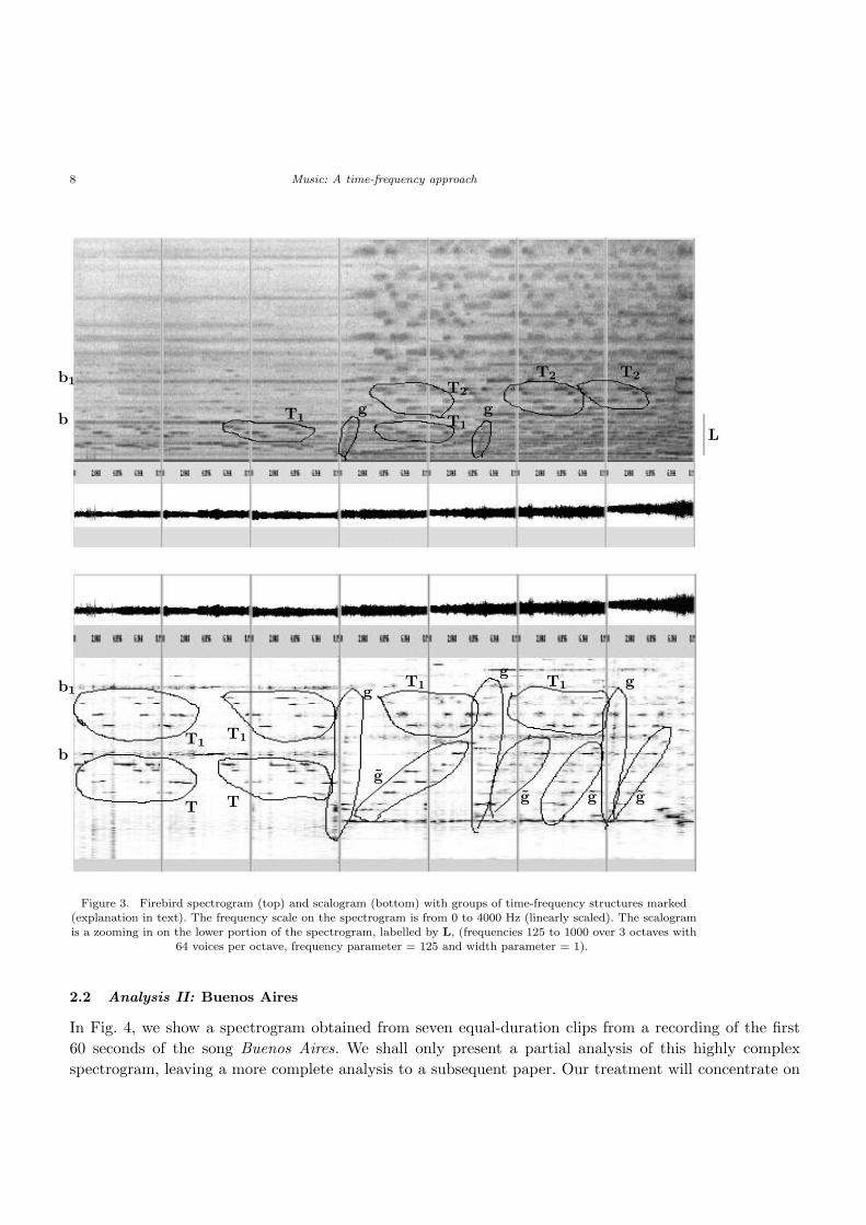
we see that the first three panels of the spectrogram in Fig. 3 contain the horn solo playing the notes of

the theme for the ending passage. Its last four panels contain various orchestral ornamentations combined

with a flute playing the notes of the main theme.

The higher frequency portion of these last four panels mostly appear to be overtones of fundamentals

contained within the lower frequency band marked by L on the right of the spectrogram. To zoom in on

this lower frequency band, we computed the scalogram shown at the bottom of Fig. 3.

We have marked important time-frequency structures in Fig. 3. On the first three panels on the left

of the scalogram we have enclosed two structures labelled T and their overtones labelled T1. These are

the notes of the horn playing the main theme twice. The second overtone structure T1, corresponding to

the overtones of the second playing of the theme, is also marked in the third panel of the spectrogram.

Within the last four panels of the scalogram and spectrogram, we can see this theme repeated at higher

frequencies—structures labelled T1 and T2—which correspond to the notes of the theme played first by

violins at a higher pitch than the horn, and then joined by a flute at even higher pitch (where T2 contains

fundamentals for the flute and first overtones for the violins).

The horn solo in the first three panels is underlayed by a faint string accompaniment providing a constant

tonal background. This background tone appears as line segments, labelled b for the fundamental and b1

for the first overtone, in both the spectrogram and scalogram. This faint accompaniment disappears in the

last four panels, but is replaced by a complex orchestral accompaniment.

The beginning of the complex orchestral accompaniment is announced by a harp glissando, labelled g,

at the beginning of the fourth panel in both spectrogram and scalogram. The structure labelled g, which

begins right after the first glissando g, is a prolongation of the structure g at a longer time-scale with

a more detailed structure. That it is, in fact, a prolongation of g is emphasized by part of its structure

consisting of faint harp notes in addition to string notes (we show how to selectively amplify those harp

notes in subsection 3.3). This combination of g followed by g is then repeated, at shorter time-scales, in

the last three panels. These repeated structures, however, are played by the string section of the orchestra.

Summarizing our analysis, we can say that this piece of music exemplifies our Multiresolution Principle:

repetition of patterns of time-frequency structures over multiple time-scales, and multiple levels of resolution

in the time-frequency plane. In particular, the three representations described by Pinker do occur here: (1)

the first representation, the grouping of notes, corresponds to our classification of the horn theme T, the

violin theme T1, the flute theme T2, the glissando g, and its prolongation g; (2) the second representation,

the metrical structure, is reflected in the precise timings of the repetitions of notes and themes; and (3)

the third representation, the dissection of the melody into essential parts and ornaments, is reflected in

the structures g and their prolongations g being repeatedly overlaid as ornamentations of the repeated

themes T1 and T2. Thus our time-frequency approach to music is able to meet the challenge of analysing

Stravinsky’s Firebird Suite. We again urge the reader to listen to the recording on the website (2) while

the spectrogram is traced. Our analysis enables a new appreciation of the beauty of the piece.


b

b1

L

T1g

T1

T2

g

T2 T2

b

b1

T

T1

T

T1

g

g

T1g

g

T1 g

g g

Figure 3. Firebird spectrogram (top) and scalogram (bottom) with groups of time-frequency structures marked(explanation in text). The frequency scale on the spectrogram is from 0 to 4000 Hz (linearly scaled). The scalogramis a zooming in on the lower portion of the spectrogram, labelled by L, (frequencies 125 to 1000 over 3 octaves with

64 voices per octave, frequency parameter = 125 and width parameter = 1).

2.2 Analysis II: Buenos Aires

In Fig. 4, we show a spectrogram obtained from seven equal-duration clips from a recording of the first

60 seconds of the song Buenos Aires. We shall only present a partial analysis of this highly complex

spectrogram, leaving a more complete analysis to a subsequent paper. Our treatment will concentrate on


Figure 4. Spectrogram of passage from Buenos Aires (frequency scale 0 to 4000 Hz, linearly scaled).

something new, a discussion of rhythmic aspects of the music.

Buenos Aires begins with a richly structured Latin percussion passage, rather than a tonal melody.

Although Jackendoff and Lerdahl’s theory is based in tonal music, we shall see that our time-frequency

approach has something to contribute to analysing this purely rhythmic music. The spectrogram in the

first and second panels of Fig. 4, corresponding to the percussion passage, is mostly composed of a sequence

of vertical line segments. At the top of Fig. 5 we show an expanded view of the second panel. Each vertical

line segment corresponds to a percussive strike on some drum. These sharp strikes on drum heads excite a

continuum of frequencies rather than a discrete tonal sequence of fundamentals and overtones. The rapid

onset and decay of these strikes produces vertical line segments in the time-frequency plane.

To determine what patterns lie within the sequence of time positions of these vertical line segments, we

used the following three-step process: (1) compute a signal consisting of averages of the Gabor transform

square-magnitudes for horizontal slices lying between 2000 and 3000 Hz (those slices lie in a region mostly

composed of the vertical line segments); (2) compute a signal that is 1 whenever the signal from step (1)

is larger than its mean value and 0 otherwise (this new signal tracks the time-positions of the strikes); (3)

compute a Gabor wavelet scalogram of the signal from step (2). The result of step (3) is shown at the

bottom of Fig. 5. We refer to such a scalogram as a percussion scalogram. Percussion scalograms are a new

technique that provides an objective method for analysing percussion performance.

We shall now analyse the percussion scalogram in Fig. 5. Along its top, we see many repeated singletons

similar to the one labelled S. These singletons correspond to individual strikes. For instance, listening to

the first quarter of the percussion clip, we hear several strikes corresponding to singletons.

Several of these singletons are grouped together into larger forks such as the ones we have labelled T1,

T2, . . . , T5. Those forks correspond to triplets of strikes. Listening to the third quarter of the clip, we


S T1 T2 T3 T4 T5

0 2.048 4.096 6.144 8.192sec0.25

0.707

2

5.657

16

strikessec

0

1000

2000 Hz

3000

4000

Figure 5. Top: Percussion clip from Buenos Aires. Bottom: Percussion scalogram (6 octaves, 32 voices, frequencyparameter 1, width 4, hence base frequency 0.25 strikes/sec). Labelled structures explained in text.

hear three triplets of strikes in its middle corresponding to the forks T3, T4, T5. Notice also that the fork

T3 contains a faint line segment between its two tines. Listening closely to the strikes corresponding to

that fork, we hear a more complicated series of strikes beyond just a simple triple. The fork T1 occurs

near the end of the first quarter of the clip and is narrower than the forks T3, T4, T5. Listening to the

first quarter of the clip, we hear a more quickly timed triple of strikes near its end. Finally, we note that

the fork T2 near the middle of the second quarter of the time-interval corresponds to a triple of strikes

occurring near the middle of the second quarter of the clip.

Around the middle level of the percussion scalogram, there are dark blobs lying below some singletons

and forks. For example, there are three conjoined dark blobs lying below the forks T3, T4, T5 in the

middle of the third quarter of the time interval. Moreover, we hear the triplets corresponding to these

forks as part of a larger pattern. Likewise, the conjoined dark blobs below the singletons and forks in the

fourth quarter reflect a larger pattern to the percussive sound, which we perceive on listening to the fourth

quarter of the clip. These dark blobs objectively describe the timings of the singletons and triplets. For

example, the dark blob at the base of the fork T2 is at a lower height than the three dark blobs below the

forks T3, T4, T5. Since the heights of these blobs correspond to strikes/sec, we should hear faster timing

of the three triplets in the middle of the third quarter of the clip than for the triplet in the middle of the

second quarter. Listening to these two quarters of the clip confirms this prediction.

Our percussion scalogram analysis shows how the Multiresolution Principle—patterning of time-

frequency structures over multiple time-scales—applies to this purely rhythmic portion of the music. We

can even see Pinker’s three representations applying as well, if we substitute “strikes” for “notes”. For ex-


a a a

Figure 6. Fourth and fifth panels of the spectrogram from Fig. 4 with related groups of time-frequency structuresmarked a, a, and a. Frequency scale 0 to 4000 Hz linearly scaled.

ample, singletons are grouped together into forks, and these forks are grouped together into longer patterns.

Mathematical analysis of the percussion scalogram technique that allowed us to objectively characterize

this patterning is one direction for future research.

Of course, our time-frequency approach applies to the melodic aspects of this piece as well. Since we

already dealt with a melodic example in Analysis I, we shall just make a few brief remarks here. At the

bottom of Fig. 6 we have labelled three prominent time-frequency structures, a, a, and a. The structure

a is a prolongation with ornamentation of the structure a, while a is a reduction with loss of detail of the

structure a. The components of these structures are formants, arranged in fundamentals and overtones,

corresponding to the words of the song, as sung by Madonna. They follow the note patterns of the music

since they are the lyrics of the song. Similar analyses can be applied to the rest of the spectrogram.

2.3 Analysis III: A warbler’s song

Bird song has long been appreciated for its musical qualities. See [22] for a tour-de-force discussion, and [26]

for important philosophical and musical ruminations. The website for Rothenberg’s book [27], especially the

link, What Musicians Have Done with Bird Song, contains some beautiful examples of avian-inspired music

(including duets of Rothenberg playing along with birds!). More such examples can be found at the avian

music website [4], including the use of human instruments (voice, sax) to produce time-frequency structures

similar in shape and tempo to bird songs. Chapter 5, Zoomusicology, of Francois-Bernard Mache’s classic

book [23] contains a detailed analysis of the musicality of bird song, including: (1) its relation to classical

compositions such as Stravinsky’s Rite of Spring, (2) transcriptions reminiscent of rhyming patterns for


a b c

d

b1 c1

d1

Figure 7. Spectrogram of a warbler’s song.

poetry, and (3) the use of spectrograms as a generalized musical notation. In her thesis on Gabor transforms

and music [9], Dorfler also states that “Diagrams resulting from time-frequency analysis . . . can even be

interpreted as a generalized musical notation”.

We shall analyse a song of a warbler. In Fig. 7, we show a spectrogram of a warbler’s song. Three time-

frequency structures stand out for their similarity. We have labelled these structures a, b, and c. They all

resemble fern leaves, but at larger and larger sizes in the time-frequency plane as time progresses—they

correspond to the chirps of the warbler’s song. Structure b is a larger scale version of structure a with

additional ornamentation, including some additional overtones (structure b1). Similarly, structure c is a

larger scale version of b with additional ornamentation (especially in the first overtone structure c1). Here

we have a clear example of our Multiresolution Principle, and of the three representations listed by Pinker:

(1) The first representation consists of the grouping of sound into the structures a to d; (2) the second

representation consists of the precise timings of the chirps, with each chirp lasting about the same length

of time, but growing in intensity; (3) the third representation consists of the similarity of structures a, b

and c (in fact, although the warbler does not sing with clearly defined notes, the “skeleton of the melody

is conserved while the ornaments differ from variation to variation”). While the final structure d in the

spectrogram is not a larger scale version of the previous structures, it is not completely anomalous, since

it clearly extends the trend of the “leaf structures” of b and c in the time-frequency plane. Summing up,

our sense that the warbler is creating music is in line with our time-frequency approach.

We have seen that iteration at multiple scales of a basic structure (structure a) is an important component

of the warbler’s song. We now turn to an experimental musical composition which makes explicit use of

such iteration, a fractal musical composition.

2.4 Analysis IV: fractal music

Considerable recent work by composers uses ideas from fractal theory. A lot of these new musical compo-

sitions are available on the Internet. See e.g. the websites listed in references [16,19,25]. In this section we


Figure 8. Left: spectrogram of fractal music passage. Right: scalogram of fractal music passage (frequencies 240 to480 on a 1-octave scale with 256 voices, frequency parameter = 240, width parameter = 1). This scalogram is a

zooming in on the lowest triangle in the spectrogram.

use spectrograms and scalograms to examine a musical passage generated by drawing the famous fractal

shape of Sierpinski’s triangle.

Sierpinski’s triangle can be drawn in the plane by iterating a series of randomly chosen affine transfor-

mations, starting from a given point. See [6, p. 85] for a precise description of the affine transformations

used. Reference [6] provides a particularly thorough discussion of the mathematics, so we shall not provide

more details here. Our iterations were done 2500 times using John Rahn’s Common Lisp Kernel for

music synthesis (available from the website [25]) which converts the generated fractal shape into a file of

instrumental tone parameters determining initiation, duration, and pitch. This file of instrumental tone

parameters was then converted into a digital audio file using the software C-Sound [7].

In Fig. 8, we show a spectrogram and a scalogram of this digital audio file. The left of Fig. 8 shows a

spectrogram over a linearly-scaled frequency range from 0 Hz to 1378 Hz. The lowest triangle, between

frequencies 240 Hz and 480 Hz, is an approximate Sierpinski triangle corresponding to the fundamentals

of the generated tones, above it are Sierpinski triangles corresponding to overtones. On the right of Fig. 8,

we show a scalogram that zooms in on the fundamental Sierpinski triangle from 240 Hz to 480 Hz. In this

fractal shape, we can see our Multiresolution Principle exemplified: repetition of patterns of time-frequency

structures over multiple time-scales, and multiple levels of resolution in the time-frequency plane. It also

exemplifies the first two representations described by Pinker. The first representation is exemplified by

the self-similar hierarchy of triangles that together form the full triangle, illustrating how “groups . . . hang

together in motifs, which in turn are grouped into lines or sections”. The second representation is illustrated

by the precise timings of the attacks and decays of the sub-triangles which gives rise to a ghostly chorus.

Finally, Pinker’s third representation is illustrated by the spectrogram on the left of Fig. 8 which exhibits

repetitions with ornamentations, the “skeleton of the melody is conserved while the ornaments differ from

variation to variation”.

Listening to this digital audio file, we hear an overall pitch-ascending series of ghostly voices (each voice

corresponding to a sub-triangle within the overall Sierpinski triangle) until the apex of Sierpinski’s triangle


is reached, and then a series of overall pitch-descending voices complementary to the ascending first half.

This ghostly chorus is not singing in reference to any series of notes composed using classical music theory.

Nevertheless, our time-frequency approach provides an objective basis for its musical analysis.

2.5 Counterexamples

The theory described in this section has limits, not all sounds are musical. Two cases of non-musical sounds

are (1) random environmental noise (see subsection 3.2), where there is no pattern to the time-frequency

structures; and (2) conversational speech, where there can be patterning of time-frequency structures

(e.g. formants from vocal chord vibrations), but this patterning is not structured over multiple time-scales

by the three representations. Thus in neither case do we perceive such sounds as musical.

3 Musical synthesis

In this section we examine musical synthesis based on inverting Gabor transforms. We shall see that this

inversion process allows for several important tasks in musical processing and synthesis, including the

following examples:

(i) removing environmental background noise from the warbler song, as an illustration of the funda-

mental task of digital audio restoration;

(ii) amplifying just the first prolongation g in the passage from the Firebird Suite, while leaving the

remaining music accompanying it at the same intensity, an illustration of changing figure-ground

aspects of a musical recording;

(iii) altering the timings and loudness of piano notes, while keeping a symphonic background unaltered,

to affect the mood of a composition like Rhapsody in Blue, we dub this converting Bernstein to

Gershwin;

(iv) generating new musical sounds.

3.1 Inversion of Gabor transforms

Because the frame condition (3) holds, we can invert the Gabor transform in (1) as follows. First, apply

inverse FFTs:

{F{f(tk)w(tk − τm)}}Mm=1

F−1

−→{{f(tk)w(tk − τm)}}Mm=1.

Then multiply each subsignal {f(tk)w(tk − τm)} by {w(tk − τm)} and sum over m:

{{f(tk)w(tk − τm)}}Mm=1 −→ {

M∑

m=1

f(tk)w2(tk − τm)}.


The last sum equals {f(tk)M∑

m=1

w2(tk − τm)}. Multiplying it by [M∑

m=1

w2(tk − τm)]−1, which is no larger

than A−1, we obtain {f(tk)}. Thus, we can always invert our Gabor transforms.

3.2 Synthesis I: Removing background noise

A vital task of music processing is the removal of extraneous noise from digital audio recordings. In this

subsection we discuss how Gabor transforms can be used for such denoising. There is insufficient space to

properly treat state of the art Gabor transform denoising (see [9]), but through our treatment of one test

case, we shall illustrate the main ideas involved with such methods (see [28] for more details).

In the recording of the warbler’s song discussed in subsection 2.3, there is considerable background noise,

which is most perceptible at the beginning and end of the recording where we do not hear the warbler

singing. Notice that there is no structure to the spectrogram in Fig. 7 on either the left or the right of the

structures that we identified as the warbler’s song. There is just a random array of grey pixels forming a

kind of background.

We shall adopt the standard additive noise model used in audio engineering. We assume that the signal

{f(tk)} in the recording is described by

f(tk) = g(tk) + nk

where g(tk) is the true signal, the warbler’s song uncorrupted by noise, and {nk} are independently identi-

cally distributed normal random variables of mean 0 and standard deviation σ [i.e. they are i.i.d. N (0, σ)].

Using the standard unbiased estimator from elementary statistics, we estimate that the standard deviation

of the beginning of the signal (from t = 0 to t = 0.187), where there is only noise, is σ = 2.0338138. We

shall assume that σ ≈ σ.

We now show how to denoise the signal. We make the following three observations. First, because {nk}are i.i.d. N (0, σ), we expect that more than 99.5% of the noise values nk will satisfy |nk| ≤ 3σ. Second,

because f = g + n, a Gabor transform of {f(tk)} satisfies

{F{f(tk)w(tk − τm)}}Mm=1 = {F{g(tk)w(tk − τm)}}M

m=1 + {F{nkw(tk − τm)}}Mm=1.

If a boxcar window is used, then this last equation simplifies to

{F{f(tk)}tk∈Im}M

m=1 = {F{g(tk)}tk∈Im}M

m=1 + {F{nk}tk∈Im}M

m=1

where Im is the set of values tk satisfying |tk − τm| ≤ λ/2. On the left of Fig. 9, we show this boxcar

windowed spectrogram of the noisy warbler song. Third, the FFT F used by Fawave for computing all


Figure 9. Left: Spectrogram of warbler song. Middle: spectrogram of thresholded Gabor transform. Right:spectrogram of soft-thresholded and clipped Gabor transform.

these spectrograms is given by (for all sequences {ak}N−1k=0 ):

{ak}N−1k=0

F−→{A` =N−1∑

k=0

ake−i2πk`/N}

where N = 512 is a fixed number of points. From Parseval’s equality

N−1∑

k=0

|ak|2 =1

N

N−1∑

`=0

|A`|2 (5)

we conclude that F is√

N times a unitary transformation. Moreover, since the real and imaginary parts

of F (denoted by <F and =F) are mutually orthogonal sine and cosine transformations, it follows that for

all random signals, {xk}, the real-part of the FFT, {<(X`)}, and the imaginary part of the FFT, {=(X`)},satisfy (on average, in terms of expected value):

N−1∑

`=0

|<(X`)|2 =N−1∑

`=0

|=(X`)|2 =1

2

N−1∑

`=0

|X`|2. (6)

From equations (5) and (6), we conclude that both <F and =F can be expected to behave on random sig-

nals as√

N/2 times orthogonal transformations. Hence {<F{nk}} and {=F{nk}} are i.i.d. N (0, σ√

N/2).

Therefore we expect that the transformed noise values <F{nw} and =F{nw} will have more than 99.5%

of their square-magnitudes smaller than 9σ2N/2. Putting all these observations together, we expect that

99% of the values of the noise’s Gabor transform will be smaller in magnitude than 3√

Nσ = 138.05986.

Our first attempt at denoising the warbler’s song is simply to discard (set to 0) all the values of its Gabor

transform whose magnitudes lie below the threshold 138.05986. The spectrogram for this thresholded

Gabor transform is shown in the middle of Fig. 9. As expected, the vast majority of noise values have


gX

XXz

3gX

XXz

Figure 10. Left: spectrogram of portion of Firebird Suite. Right: spectrogram with structure g amplified.

been eliminated by this thresholding. By applying the Gabor transform inversion procedure, we obtained

a denoised signal. We urge readers to listen to this denoised signal to hear how successful we were.

If one listens closely to the denoised signal, one notices a jingling tone underlying the bird call. This

jingling tone is an artifact of the “hard thresholding” we applied to the spectrogram. To remove it, we

did a second denoising, utilizing the idea of soft thresholding (also called shrinkage) from the theory of

wavelet denoising [8]. The soft thresholding described in [8] applies to orthogonal transforms. Since, on

random signals, <F and =F are mutually orthogonal multiples of orthogonal transforms, it makes sense to

apply soft thresholding to the FFT magnitudes from the Gabor transform. We applied the soft threshold

function

T (x) =

{x − 138.05986, for x > 138.05986

0, for x ≤ 138.05986

to the magnitudes of the Gabor transform of the warbler song (leaving the phases unaltered). We also

eliminated the line segment lying just to the left and near the bottom of the first “fern-leaf” structure

in the spectrogram in the middle of Fig. 9—which appeared to us to be an environmental artifact, since

it does not fit the pattern of the structures of the warbler’s call—by retaining only values for t > 0.461.

The result of these two steps is shown in the spectrogram on the right of Fig. 9. This second denoising is

relatively free of artifacts.

3.3 Synthesis II: Altering figure-ground

In [10], Dorfler mentions that one application of Gabor transforms would be to select one instrument, say

a horn, from a musical passage. Here we will illustrate this idea by amplifying the first prolongation of the

glissando, structure g, in the passage from the Firebird Suite analysed in subsection 2.1.

We show on the left of Fig. 10 a spectrogram of a clipping of a portion of the Firebird Suite recording,


where we have marked the structure g. To amplify just this portion of the sound, we multiply the Gabor

transform values by a mask of value 3 within a narrow parallelogram containing g and value 1 outside the

parallelogram (see the right of Fig. 10), and then perform the inverse transform. Notice that the structure

3g stands out more from the background of the remainder of the spectrogram (which is unaltered).

Listening to the processed sound file we hear a much greater emphasis on the harp notes than in the

original. We have altered the figure-ground relationship of the music.

The modification we have performed in this example is a joint time-frequency filtering of the Gabor

transform. It cannot be performed as a frequency domain filtering typically employed by sound engineers

(due to the sloping of the structure g in the time-frequency plane), nor can it be executed purely in the

time-domain. With this example, we have touched on an important field of mathematical research known

as Gabor multipliers. More details can be found in reference [12].

3.4 Synthesis III: Converting Bernstein to Gershwin

In this subsection we describe a dream for future research and development. Consider a recording of

Leonard Bernstein playing piano for Rhapsody in Blue, accompanied by the New York Philharmonic.

Bernstein’s playing is less jazzy in spirit than say George Gershwin’s. If we could isolate the structures in a

spectrogram of the Bernstein recording that correspond to the piano notes (like we isolated the structures

for the horn notes at the beginning of the Firebird Suite passage shown at the top of Fig. 3), then we could

modify the Gabor transform as follows. We could slightly perturb in time (backwards or forwards) the

Gabor transform values corresponding to the piano notes thus altering slightly the timings of Bernstein’s

key strikes. We could also multiply those Gabor transform values by various constants for each note played

to alter the emphasis of Bernstein’s key strikes. In this way we could “jazz up” Bernstein’s playing and

perhaps convert it to more like the style of George Gershwin. We would have converted Bernstein to

Gershwin, while keeping the symphonic background unaltered. George Gershwin would be playing with

the New York Philharmonic instead of Leonard Bernstein.

Clearly there are many technical difficulties that need to be resolved in order for this dream to be

realized. Nevertheless, we believe it offers great potential.

3.5 Synthesis IV: New musical sounds from Gabor transforms

Our final example uses the inverse Gabor transform, in conjunction with ideas from the musical theory

described in Section 2, to create an artificial bird song. This only partially realizes the goal of creating

new music with Gabor transforms, but it is a start.

We begin by creating an artificial bird chirp. In Fig. 11(a) we show the spectrogram of a single chirp

of an oriole. To create our artificial bird chirp we formed a time-frequency matrix of magnitudes, shown

in Fig. 11(b). It consists of a combination of a thickened parabolic segment attached to two thickened

line segments—drawn using the spectrogram plotting procedure of Fawave∗. By performing an inverse

∗Complete details of this plotting procedure are provided at the article webpage (2).


(a) (b) (c)

Figure 11. (a) Oriole chirp. (b) Synthesized bird chirp. (c) Synthesized bird song.

Gabor transform on those magnitudes (phase angles all set to 0), we created an artificial bird chirp. It

is interesting that, even though no phase information was used, the specification of time locations and

magnitudes shown in Fig. 11(b) was sufficient to create a reasonably natural sounding bird chirp.

Our final step was to create an artificial bird song by repeating the process just described. See Fig. 11(c).

To produce this graph we repeated the time-frequency structure in Fig. 11(b) twice more at successively

shrunken time-scales, followed by three more repetitions at a much shorter time-scale and translated

upward in frequency. Our time-frequency approach predicts that a signal with such a time-frequency

graph will sound musical. Indeed, the synthesized signal, obtained by Gabor transform inversion, does

sound like a bird song.

Clearly, this bird song example is just a beginning. We will continue, however, to investigate the synthesis

of new musical sounds using inverse Gabor transforms. We will also investigate how our time-frequency

approach to music can be developed with some of the newest methods of time-frequency analysis, such as

localized Gabor frames [9, 11, 29], and reassigned short-time Fourier transforms [17].

References

[1] Alm, J. and Walker, J., 2002, Time-frequency analysis of musical instruments. SIAM Review, 44, 457–476. Available athttp://siamdl.aip.org/dbt/dbt.jsp?KEY=SIREAD&Volume=44&Issue=3

[2] Assayag, G., Feichtinger, H. and Rodrigues, J.-F. (Eds.), 2002, Mathematics and music: a Diderot Mathematical Forum. Springer,New York.

[3] Audacity is available at http://audacity.sourceforge.net/

[4] Avian music webpage: http://www.avianmusic.com/[5] Balazs, P. et al., 2006, Double preconditioning for Gabor frames. To appear in IEEE Trans. on Signal Processing. Available at

http://www.unet.univie.ac.at/~a8927259/wissenen.html

[6] Barnsley, M., 1993, Fractals Everywhere, Second Edition. Academic Press, Cambridge, MA.[7] C-Sound is available at http://www.csounds.com/

[8] Donoho, D. et al., 1995, Wavelet shrinkage: asymptopia? J. of Royal Stat. Soc. B, 57, 301–369.[9] Dorfler, M., 2002, Gabor Analysis for a Class of Signals called Music. Dissertation, University of Vienna. Available at

http://www.mat.univie.ac.at/~moni/

[10] Dorfler, M., 2001, Time-Frequency Analysis for Music Signals—a Mathematical Approach. J. of New Music Research, 30, 3–12.Available at http://www.mat.univie.ac.at/~moni/

[11] Dorfler, M. and Feichtinger, H., 2004, Quilted Gabor Families I: Reduced Multi-Gabor Frames. Appl. Comput. Harmon. Anal., 356,

2001–2023. Available at http://www.mat.univie.ac.at/~moni/

[12] Feichtinger, H. and Nowak, K., 2003, A First Survey of Gabor Multipliers. In Feichtinger, H. and Strohmer, T. (Eds.), Advances inGabor Analysis. Birkhauser, Boston. Available at http://www.univie.ac.at/nuhag-php/home/feipub_db.php


[13] Feichtinger, H. and Strohmer, T. (Eds.), 1998, Gabor Analysis and Algorithms. Birkauser, Boston, MA.[14] Feichtinger, H. and Strohmer, T. (Eds.), 2003, Advances in Gabor Analysis. Birkauser, Boston, MA.[15] Flandrin, P., 1999, Time-Frequency/Time-Scale Analysis. Academic Press, San Diego, CA.[16] Fractal music webpage: http://www.fractalmusiclab.com/default.asp[17] Gardner, T. and Magnasco, M., 2006, Sparse time-frequency representations. Proc. Nat. Acad. Sci., 103, 6094–6099. Available at

http://www.pnas.org/cgi/reprint/103/16/6094.pdf

[18] Grochenig, K., 2001, Foundations of Time-Frequency Analysis. Birkhauser, Boston, MA.[19] Hatzis, C., webpage: http://www.chass.utoronto.ca/~chatzis/[20] Jackendoff, R. and Lerdahl, F., 1983, A Generative Theory of Tonal Music. MIT Press, Cambridge, MA.[21] Lerdahl, F. and Jackendoff, R., 1992, An Overview of Hierarchical Structure in Music. In Schwanauer, S. and Levitt, D. (Eds.),

Machine Models of Music, MIT Press, Cambridge, MA, 289–312.[22] Kroodsma, D., 2005, The Singing Life of Birds. Houghton-Mifflin, NY.[23] Mache, F., 1993, Music, Myth and Nature. Contemporary Music Studies, Vol. 6. Taylor & Francis, London.[24] Pinker, S., 1997, How the Mind Works. Norton, NY.[25] Rahn, J., webpage: http://faculty.washington.edu/~jrahn/[26] Rothenberg, D., 2005, Why Birds Sing: A Journey Into the Mystery of Bird Song. Basic Books, NY.[27] Rothenberg, D., Why Birds Sing webpage: http://www.whybirdssing.com/[28] Walker, J., 2006, Denoising Gabor transforms. Submitted. Available at http://www.uwec.edu/walkerjs/TFAM/DGT.pdf

[29] Zheng, Z. and Feichtinger, H., 2000, Gabor eigenspace time-variant filter. In Proc. 2000 IEEE Electro/Information TechnologyConference, Chicago, USA.

music: a time-frequency approach - university of … · 2009-01-03 · music: a time-frequency...

Documents