my referred paper

International Electronic Journal of Pure and Applied Mathematics——————————————————————————————Volume 1 No. 3 2010, 303-337

BIFURCATION AND CHAOS IN

HIGHER DIMENSIONAL PIONEER-CLIMAX SYSTEMS

Yogesh Joshi1 §, Denis Blackmore2

1,2Department of Mathematical SciencesNew Jersey Institute of Technology

Newark, NJ 07102-1982, USA1e-mail: [email protected]

2e-mail: [email protected]

Abstract: A discrete dynamical model is formulated for the evolution of a bi-ological system comprised of pioneer and climax species. This hierarchical modelgeneralizes a well-known two-dimensional system for pioneer-climax species thatprovides reliable predictions for actual ecological systems. An extensive dynami-cal systems investigation is conducted using analytical and simulation tools. It isproved, for example, that the model has no Hopf bifurcations, but exhibits a richarray of flip (period-doubling) bifurcations for various (parameter) codimensions. Akey to proving this and other results is that the hierarchical nature of the modelmakes it essentially equivalent to a sequence of one-dimensional systems when itcomes to several dynamical properties (hierarchical principle). For example, thisprinciple is used to prove chaos in the limit of a period-doubling cascade, shift mapchaos on an invariant two-component Cantor set when there is a climax component,and the existence of an interesting small scale strange attractor like set when thereis a pioneer component. Bifurcation diagrams and Lyapunov exponents are com-puted to further illustrate the chaotic dynamics, and it is indicated how chaos canbe proved using higher dimensional horseshoe maps.

AMS Subject Classification: 37C05, 37G10, 37N25, 92D25Key Words: pioneer and climax species, hierarchical principle, flip bifurcation,bifurcation diagrams, chaos, Lyapunov exponents

Received: June 8, 2010 c© 2010 Academic Publications§Correspondence author

Inte

rnati

onalEle

ctr

onic

Journ

alofP

ure

and

Applied

Math

em

ati

cs

–IE

JPA

M,V

olu

me

1,N

o.3

(2010)

304 Y. Joshi, D. Blackmore

1. Introduction

Pioneer and climax species, which usually refer to types of flora, have been studiedfor many years by both ecologists and applied mathematicians, and more recentlyhave been extensively investigated using a variety of dynamical systems models,most of which have been limited to two-dimensional (two-species) models. Thosespecies that first colonize a barren land are called pioneer species. They are veryhardy species that have adapted themselves to harsh conditions of nature, suchas soil with less water retaining properties, and an overall dearth of water. Tosurvive such harsh environments, in the course of time they tend to develop longerroots, leaves that transpire less, and other such adaptations. They are also theones that usually grow first in an ecosystem which is destroyed by a forest fire,flood, earthquake, volcanic eruption or human intervention such as clearance ofland for development and mining. They grow rapidly, but excessive increases intheir density are detrimental to their own growth, leading ultimately to extinction.As the ecosystem grows with time, new species called climax species take over fromthe pioneer species. They now share the environment which was first occupied bythe pioneer species. But they take more time to grow. The initial low density ofclimax species enhances their growth. Once they attain their maximum density, theirgrowth rate starts to decline. Some examples of pioneer species are weeds, marramgrass, some types of Pine and Poplar trees, wind-dispersed microbes, mosses andlichens that grow close to the ground. Hardwood trees like Oak, Maple, and WhiteSpruce are examples of climax species [17], [18], [24].

Many experimental studies (field work) have also been conducted, with [8], [13],[14], [22] being some of the more recent ones. In [8], Jegan, Ramesh and Muthuche-lian showed that pioneer species need light for regeneration and resprouting whichare important processes that allow plant species to remain viable in an ecosystem,but which climax species do not require to the same extent. They evolve in anenvironment that is made easy to grow and thrive in by their predecessors, whichare typically pioneer species. Jegan et al [8] classified their results based on forestopenings (closed, small gap and large gap) which played a pivotal role in the study.

Raaimakers et al [13] investigated whether low phosphorous (P) availability lim-its the process of photosynthesis more than nitrogen (N) does in tree species inGuyana where the soil quality is acidic. The experiment was carried on nine pio-neer and climax tree species. They also studied the relationship between leaf P andN content with photosynthetic capacity. They found at similar P and N content,pioneer species have a higher photosynthetic capacity than the climax species in arange of light climates. Photosynthetic characteristics and pattern of biomass accu-mulation in seedlings of pioneer and climax tree species from Brazil were studied bySilvestrini et al [22]. The seedlings were grown for four months under low light (5% to8% sunlight) and high light (100% sunlight). Both species exhibited characteristicsthat favor growth under conditions that resemble their natural microenvironments.In

tern

ati

onalEle

ctr

onic

Journ

alofP

ure

and

Applied

Math

em

ati

cs

–IE

JPA

M,V

olu

me

1,N

o.3

(2010)

BIFURCATION AND CHAOS IN... 305

They also found that the climax species grow under high light, which is not normallyobserved in climax species. They proposed to explain this behavior using the spatio-temporal light regime of the forest. In [11], Kuijk developed and used a model forforest regeneration and restoration in Vietnam. The model evaluates shoot heightand plant architecture, biomass allocation patterns and leaf physiology in terms oflight capture and photosynthetic gains. Kuijk’s model proved to be quite successfulwhen applied to grasslands. Forest regeneration is a successional process where oldtrees (pioneers) are replaced by the new ones (climax) and a structural change inthe forest canopy occurs.

From the applied mathematical perspective, the challenge is to formulate dynam-ical models for the evolution of ecosystems comprised of pioneer and climax speciesthat can be used to reliably predict the behavior described above as well as a rangeof other qualitative and quantitative properties. Such models are usually either con-tinuous or discrete dynamical systems, and the predictions are made using a varietyof theoretical and computational tools that have been developed to analyze thesemodels. Our approach here is to study a discrete dynamical systems model that isa higher dimensional generalization of a two-species system introduced by Selgradeand Namkoong [17, 18], which has proven to be quite successful in predicting thebehavior of a pair of such species.

2. The Model

In an ecosystem, there are many interactions taking place such as animal-animal,plant-plant, and plant-animal that lead either to decline and possible extinctionof one or more species (survival of the fittest) or coexistence (symbiosis). Therealso is another scenario, where some particular species of plants survive the harshconditions (pioneer) of the environment and later on become extinct after making theenvironment more friendly for other species (climax), thus increasing their chancesfor survival. In the jargon of ecology this is called succession. Then after attainingmaximum density, the climax species typically also start to dwindle. For moredetails, see [17], [18], [24].

This paper is inspired by the work of such researchers as Selgrade & Namkoong[17], [18], Franke & Yakubu [4], Sumner [23], [24], and Hassell & Comins [6] whohave conducted extensive investigations of two-dimensional pioneer-climax systems.These authors usually combine all the individual population densities xi of thespecies into a single entity, called the total weighted density, zi =

∑mj=1 cijxi,

where the |cij | represent the intensity of the effect of the j-th population on thei-th. This helps to take into account all the competition (both interspecies andintraspecies) which takes place among the species. The cij are often called the in-

teraction coefficients, and the cii are invariably chosen as positive numbers. So,while modeling an individual species, we will consider per capita growth rates to beIn

tern

ati

onalEle

ctr

onic

Journ

alofP

ure

and

Applied

Math

em

ati

cs

–IE

JPA

M,V

olu

me

1,N

o.3

(2010)


functions of total weighted density. The per capita growth rate is called the fitness

function, which can have the form

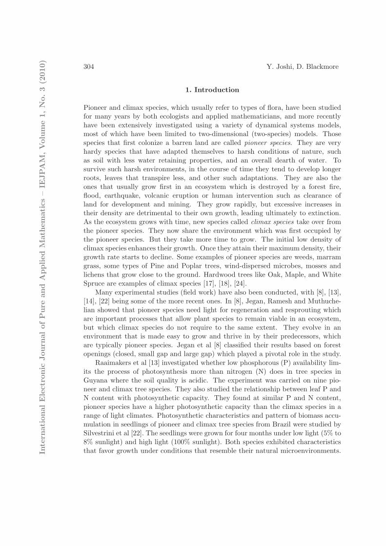
φ(x) = xαea−x,

and is shown in Figure 1, where α = 0 or 1 according as the species is pioneer orclimax, respectively, and a is a positive parameter describing the growth rate ea

of the species. For the i-th species to be a pioneer, it is required that the fitnessfunction φi be smooth, monotonically decreasing and satisfies φi(0) > 1. On theother hand, the species is climax if φi is smooth, initially monotonically increas-ing, reaches some maximum per capita growth rate, and deceases monotonicallythereafter. Note that the density of species i is given as xiφi(xi). Typical growthof pioneer and climax species is shown in Figure 1. A widely accepted and stud-ied 2-species pioneer-climax discrete dynamical model was introduced in Selgradeand Namkoong [17], [18]. Extending it to higher dimensions, we take the followingm-dimensional pioneer-climax model (m > 2) as our starting point:

xi(n + 1) = xi(n)zi(n)αiea−zi(n), (1 ≤ i ≤ m)

where

zi =m∑

j=1

cijxj ,

is the total weighted density, with ai, cij > 0 and all zαi

i ≥ 0 whenever all x1, . . . , xmare nonnegative.

To make our results more relevant to real world ecosystems, we shall concentrateour attention by imposing hierarchical competition [2] on our model. In hierarchicalcompetition, species i affects the growth of another species j if the j-th species liesbelow the i-th in the food chain of the ecosystem under consideration. To be moreprecise, our hierarchical pioneer-climax model (HPCM) assumes the form

xi(n+ 1) = xi(n)(

∑i

j=1cijxj(n)

)αi

exp(

ai −∑i

j=1cijxj(n)

)

(1)

(1 ≤ i ≤ m). The system may be recast into discrete dynamical form in terms ofthe iterates of a smooth (= C∞) map – which is actually real-analytic (= Cω) – bydefining Fα,ν : Rm

+ → Rm+ as

Fα,ν(x) = (f1α,ν(x1), f2α,ν(x1, x2), . . . , fmα,ν(x)) := (x1 (c11x1)α1

× exp (a1 − c11x1) , . . . , xm(

Pmj=1cijxj

)αm exp(

am − Pmj=1cijxj

))

, (2)

where x := (x1, . . . , xm) ∈ Rm+ := {x ∈ Rm : x1, . . . , xm ≥ 0}, α := (α1, . . . , αm),

and the parameters are all grouped into µ := (a1, . . . , am, c11, c12, . . . , c1m, . . . , cm1,Inte

rnati

onalEle

ctr

onic

Journ

alofP

ure

and

Applied

Math

em

ati

cs

–IE

JPA

M,V

olu

me

1,N

o.3

(2010)


0 1 2 3 4 5 6 70

0.2

0.4

0.6

0.8

1

1.2

1.4

1.6

1.8

Density (x)

Fitn

ess

Fun

ctio

n =

e(a

−x)

(a) Pioneer growth, with parameter a = 0.5

0 1 2 3 4 5 6 70

0.2

0.4

0.6

0.8

1

1.2

1.4

Density (x)

Fitn

ess

Fun

ctio

n =

xe(a

−x)

(b) Climax growth, with parameter a = 1.2

Figure 1: Growth of pioneer and climax species

cm2, . . . , cmm). With this, we may rewrite (1) in difference/discrete dynamical sys-tem form as

xn+1 = Fα,ν(xn) ⇐⇒ xn = Fnα,ν(x0), (3)

where Fnα,ν denotes the usual n-fold composition of Fα,ν with itself, which is defined

for all nonnegative integers and for negative integers when the inverse Fnα,ν exists.

We note here for future reference that the subscripts α and µ can and will be omittedwhen they are given and fixed for a particular investigation.

Inte

rnati

onalEle

ctr

onic

Journ

alofP

ure

and

Applied

Math

em

ati

cs

–IE

JPA

M,V

olu

me

1,N

o.3

(2010)


3. Basic Dynamical Properties

In this section we explore some basic dynamical properties of our HPCM includingsimplifications, invariant sets, stability of fixed points and the like. We shall alsodescribe how the hierarchical nature of the system reduces many dynamical consid-erations to one-dimensional maps obtained from the coordinate functions of (2). Byway of simplification, it is easy to see that our map (2) is conjugate via the simplescaling h(x1, . . . , xm) := (x1/c11, . . . , xm/cmm) to a map of precisely the same formwith

(U) c11 = c22 = · · · = cmm = 1,

so we shall assume this to be the case from this point onward.

3.1. Invariant Sets

It is clear that the map (2) is actually defined on all of Euclidean m-space Rm,and it follows directly from our assumptions that Fα,ν(Rm

+ ) = Rm+ , so Rm

+ is Fα,ν-invariant, as well it should be since there should be no populations of negative size.Moreover, it is obvious from (2) that the origin, and all of the coordinate lines, planesand hyperplanes xi1 = xi2 = · · · = xik = 0, where i1, i2, . . . , ik, with 1 ≤ k < m, isany selection of k distinct elements of the set {1, 2, . . . ,m} are F -invariant. Thereappear to be no other subsets that are obviously invariant by inspection withoutadditional specializing restrictions on F .

3.2. Fixed Points

As noted above, the origin is obviously a fixed point of F for any choice of α andthe parameter µ. Any additional fixed points are, by definition, solutions of

x = F (x) ⇐⇒ xi = xi

(

∑i

j=1cijxj

)αi

exp(

ai −∑i

j=1cijxj

)

(4)

(1 ≤ i ≤ m). Thus if xi 6= 0, it must follow that

(

∑i

j=1cijxj

)αi

exp(

ai −∑i

j=1cijxj

)

= 1,

which in the case of a pioneer component (αi = 0) is easily seen to be equivalent to

∑i

j=1cijxj = ai; (5)

on the other hand, when the component is climax (αi = 1), one finds that

∑i

j=1cijxj = V −1

(

e−ai)

= −W(

−e−ai)

, (6)Inte

rnati

onalEle

ctr

onic

Journ

alofP

ure

and

Applied

Math

em

ati

cs

–IE

JPA

M,V

olu

me

1,N

o.3

(2010)


as long as ai ≥ 1 so that the “inverse” V −1 of the function V (s) = se−s is definedfor s ≥ 0. Observe that V −1(u) = −W (−u), where W is the Lambert function [25],and V −1(0) = 0, V −1(e−1) = 1 and V −1(u) = {sl(u), sr(u)} when 0 < u < e−1,with 0 < sl < 1 < sr, and sl ↓ 0 and sr ↑ ∞ as u ↓ 0.

In virtue of (4)-(6), finding the fixed points of F is a simple matter of solvinga system of linear equations. We now consider a couple examples to illustrate this.Suppose first that all of the coordinate functions are pioneer (the all-pioneer case).Then it is easy to show, keeping in mind the assumption (U), that the unique fixedpoint with all nonzero coordinates is (x1, . . . , xm) = (a1, (a2 − c21a1), . . . , (am −cm1x1 − · · · − cm,m−1xm−1)). As another example, we consider a 3-dimensionalsystem in which the first two species are pioneer and the third is climax with a3 > 1.In this case there are a pair of fixed points with all nonzero coordinates; namely(x1, x2, x3) = (a1, (a2−c21x1), (sl(e

−a3)−c31x1−c32x2)) and (x1, x2, x3) = (a1, (a2−c21x1), (sr(e

−a3)−c31x1−c32x2)). In a similar fashion, all fixed points of the HPCMinvolving any combination of pioneer and climax species can be computed.

The linear stability of any fixed point of the system is determined from a spectralanalysis of the derivative (Jacobian) m×m matrix

F ′α,ν(x) =

(

∂xjfiα,ν(x1, . . . , xi)

)

. (7)

This is a lower triangular matrix since ∂xjfiα,ν(x1, . . . , xi) = 0 when i < j; the

diagonal entries (which are the eigenvalues) are

∂xifiα,ν(x1, . . . , xi) =

(1 − ciixi) exp(

ai −∑i

j=1cijxj

)

, αi = 0;

(

∑i

j=1cijxj

)

ciixi + (1 − ciixi)(

i∑

j=1

cijxj)

× exp(

ai −∑i

j=1cijxj

)

, αi = 1.

and the entries below the diagonal (i > j) are

∂xjfiα,ν(x1, . . . , xi) =

−cijxi exp(

ai −∑i

j=1cijxj

)

, αi = 0;

cijxi

(

1 −∑i

j=1cijxj

)

× exp(

ai −∑i

j=1cijxj

)

, αi = 1.

Using formula (7) and the diagonal entries (see above), it is easy to characterize thelinear stability of any fixed point of Fα,ν, thereby obtaining a complete set of resultsof which the following two are just examples:

Inte

rnati

onalEle

ctr

onic

Journ

alofP

ure

and

Applied

Math

em

ati

cs

–IE

JPA

M,V

olu

me

1,N

o.3

(2010)


Lemma 3.1. For the m-dimensional all-pioneer model, the origin x = 0 is arepeller (attractor) if a1, . . . , am > 0 (a1, . . . , am < 0), and for the all-climax case,the origin is superstable (all eigenvalues zero) for all values of a1, . . . , am.

Lemma 3.2. For the m-dimensional all-pioneer HPCM, the unique fixed pointwith positive coordinates (x1, . . . , xm) described above is stable if |1 − xi| < 1 forall 1 ≤ i ≤ m, and unstable if any of |1 − xi| > 1.

3.3. Possible Bifurcations

As is usual, we are interested in bifurcations of our dynamical system caused byvariation of the parameters. We show in the next section that flip (period-doubling)bifurcations are quite ubiquitous for the HPCM. However, most other standardbifurcations cannot occur, and this includes the (codimension-1) Andronov-Hopf (orNeimark-Sacker) bifurcation, which occurs in numerous other dynamical systemsmodels of physical and biological phenomena.

Lemma 3.3. There are no Hopf bifurcations for the HPCM.

Proof. It follows from (3.2) that all eigenvalues of F ′α,ν are real, which precludes

the existence of Hopf bifurcations.We note here that it is actually not too difficult prove that a general (non-

hierarchical) discrete dynamical system of pioneer-climax evolution of the type underconsideration here cannot have a Hopf bifurcation if all of the interaction coefficientsare nonnegative. However, since this does not really play any role in the sequel,we prefer not to go into this here. On the other hand, if some of the interactioncoefficients are negative, the system can experience an Andronov-Hopf (or Neimark-Sacker) bifurcation as illustrated in the following (cf. [24]):

Example 3.4. Consider F : R2+ → R2

+ defined as

F (x, y;µ) := (x exp ((8/3) + µ− x− y) , y exp ((4/3) + (µ/2) + x− y)) ,

where µ is just a real number. It is straightforward to verify that this map has asupercritical Hopf bifurcation for the fixed point (2/3, 2) at µ = 0.

3.4. The Hierarchical Principle

Owing to the hierarchical nature of the map Fα,ν, the analysis of several importantdynamical aspects of the system (3) can be reduced to a sequence of calculationsinvolving the (1-dimensional) coordinate functions of the map. This amounts towhat is essentially a reduction of the analysis of an m-dimensional system to thatof a 1-dimensional system as a result of the hierarchical structure. We shall in thesequel make extensive use of this property, which we call the hierarchical principle,or h-principle. Let us describe how this h-principle works for fixed points, periodicIn

tern

ati

onalEle

ctr

onic

Journ

alofP

ure

and

Applied

Math

em

ati

cs

–IE

JPA

M,V

olu

me

1,N

o.3

(2010)


points, and the existence of chaotic regimes, and leave it to the reader to fathomthe analogs for other types of dynamical phenomena such as bifurcations.

First, suppose we wish to find a fixed point of the system. We may start byobtaining a fixed point of the 1-dimensional first coordinate function f1α,ν, thensubstituting this, call it x1, in the second coordinate function f2α,ν to get a 1-dimensional map depending only on x2, for which we find a fixed point x2. Thenwe substitute x1 and x2 into f3α,ν to obtain a function only of x3. Repeating thisprocess until we exhaust the list of coordinate functions, we obtain a fixed point(x1, x2, . . . , xm) of Fα,ν, and all of its fixed points can be obtained in this manner.Now there is nothing special about starting with the first coordinate function: As-suming the (x1, . . . , xk−1) is a fixed point of the (k − 1)-dimensional map definedby the first (k − 1) coordinate functions of Fα,ν, we can pick up the above processby substituting x1, . . . , xk−1 in fkα,ν to obtain a function only of xk. Then we canfind a fixed point of this map, substitute it in the next coordinate map, and so onto obtain a fixed point for (2).

To find a periodic point of Fα,ν of (least) period k, it suffices to observe that F kα,ν

also is hierarchical. Accordingly the period k points can be computed as fixed pointsof F k

α,ν in the same succession of 1-dimensional calculations as described for fixedpoints of Fα,ν, and once again we essentially have a reduction from m-dimensionsto 1-dimension as a result of the hierarchical structure. Finally, it is easy to see thatchaos for the full system is generated by chaos in any of the coordinate maps, sayfkα,ν. All we need do is set (x1, . . . , xk−1) = (0, . . . , 0), which is a fixed point for themap defined by the first (k−1) coordinate functions, and consider the 1-dimensionalmap fk(xk) := fkα,ν(0, . . . , 0, xk). Then a chaotic orbit for fk naturally leads to achaotic orbit for Fα,ν, the simplest of which has xk+1 = · · · = xm = 0.

4. Period-Doubling Bifurcation

We shall now study the most significant bifurcations that can occur in the HPCMat considerable length. In order to simplify the analysis here and in succeedingsections, we shall confine our attention to 3-dimensional pioneer-climax systems,wherein we redesignate a1, a2 and a3 as a, b and c, respectively. This entails no realloss of generality, for all of our results and conclusions can be extended to the m-dimensional case in an entirely straightforward fashion.

As mentioned above, most of the interesting bifurcation behavior of the HPCMis confined to period-doubling bifurcations. The phenomenon of a period-doubling

bifurcation (or flip bifurcation) occurs in many discrete dynamical systems, andwe expect it to occur in our model based upon numerous numerical simulationsand experimental evidence. In period-doubling bifurcation, a fixed point becomesunstable (stable) and creates a stable (unstable) 2-cycle. Well-known criteria forsuch bifurcations are given in the following result (see [26]):In

tern

ati

onalEle

ctr

onic

Journ

alofP

ure

and

Applied

Math

em

ati

cs

–IE

JPA

M,V

olu

me

1,N

o.3

(2010)


Theorem 4.1. The following are sufficient conditions for the occurrence ofa period-doubling bifurcation in a 1-parameter family of Cr(r ≥ 3) 1-dimensionalmaps

x(k + 1) = f(x(k), µ), x ∈ R, µ ∈ R, k ≥ 0 :

f(x∗, µ∗) = x∗, fx(x∗, µ∗) = −1, f2µ(x

∗, µ∗) = 0, f2xx(x

∗, µ∗) = 0, f2xµ(x

∗, µ∗) 6= 0,and f2

xxx(x∗, µ∗) 6= 0, where x∗ is the fixed point and µ∗ is the bifurcation value.

We now study flip bifurcations in detail: starting with the one-dimensional modeland then generalizing the result to the 3-dimensional case in a step-by-step manner.In light of the h-principle, it makes sense to begin by considering 1-dimensionalpioneer and climax maps represented in the form f, g : R+ → R+, where

f(x) = f(x; a) := xea−x (8)

and

g(x) = g(x; a) := x2ea−x (9)

respectively where a is a positive parameter that we vary, and we have taken (U)into account. For our analysis of flip bifurcations, we could use Theorem 4.1, but weshall find it more convenient to provide direct proofs – revealing more aspects of thedynamics – that take full advantage of the special forms of the maps (8) and (9).

First, we characterize the fixed points of the two functions. Lemma 4.2. The

map f given by (8) has precisely two fixed points: x = 0 and x = a, with f ′(0) =ea and f ′(a) = 1 − a, so the origin is always unstable, and a is stable (unstable)if |1− a| is less than (greater than) one. On the other hand, the function (9) alwayshas 0 as a superstable fixed point, and this is the only fixed point if a < 1. If a =1, g also has the fixed point x = 1, with g′(1) = 1 which is unstable from the left, butstable from the right. If a > 1, g has the superstable fixed point 0, and an unstablefixed point at the smaller of the two positive solutions xl of

xea−x = 1

for which 0 < xl < 1, and another fixed point xr at the larger of the two solu-tions (xr > 1), which is stable or unstable according as the absolute value of g′(xr) =xr(2 − xr)e

a−xr is less than or greater than one, respectively.

Proof. The solutions of

f(x) = xea−x = x,

are obviously x = 0 and x = a, which are the fixed points of f . The stability resultsfor these fixed points of f follows from the formula for the derivative

f ′(x) = (1 − x)ea−x.Inte

rnati

onalEle

ctr

onic

Journ

alofP

ure

and

Applied

Math

em

ati

cs

–IE

JPA

M,V

olu

me

1,N

o.3

(2010)


The fixed points of g are the nonnegative solutions of

g(x) = x2ea−x = x,

so x = 0 is always a solution. For positive solutions, we can divide the above by x toobtain

h(x) := xea−x = 1.

A simple calculation shows that the maximum of h is ea−1, which occurs at x =1. The remaining results concerning the positive fixed points of g follow from thisformula, the derivative

g′(x) = x(2 − x)ea−x

and a simple cobweb argument for the fixed point xl, so the proof is complete.

A necessary condition for a flip bifurcation to occur at a fixed point is that thederivative be equal to −1. Relevant to this is our next result, which follows directlyfrom Lemma 4.1 and the above proof. We leave the elementary verification to thereader.

Lemma 4.3. The fixed point a is stable for 0 < a < 2. The derivative f ′(a) =−1 at a = 2, and decreases thereafter, so a is unstable for a > 2. The deriva-tive g′(xr) is a decreasing function of a, starting at g′(xr) = 1 when a = 1 andxl = xr = 1, and g′(xr) → −∞ as a → ∞. Consequently, there is a unique valueof a > 1 where g′(xr) = −1; namely, xr = 3, which corresponds to a = 3 − ln 3.

We next prove that a supercritical flip bifurcation occurs at the fixed pointsof f and g at which derivatives are equal to −1. Recall that by supercritical wemean that a fixed point transitions from stable to unstable across the bifurcationvalue of a, and gives birth to a stable 2-cycle.

Theorem 4.4. Both the pioneer map f(x) = xea−x and the climax map g(x) =x2ea−x have supercritical flip bifurcations at their largest fixed points given by xp =a and xc = 3, respectively, when f ′(xp) = −1 and g′(xc) = −1 for a = 2 and a =3 − ln 3.

Proof. We give the proof only for the pioneer case since the argument for theclimax function is completely analogous (although admittedly rather more compli-cated). Thus, we only deal with the bifurcation at the fixed point x = a of f(x) =xea−x as the parameter crosses a = 2. To show the flip bifurcation, we study f and f2,where

f2(x) := f(f(x)) = (xea−x) exp(a− xea−x)

for a > 2. Of course, as x = a is a fixed point of f , it is also a fixed point of f2. Itfollows from Lemma 4.3 that f has a unique fixed point in a neighborhood of x =a, and x = a is an unstable fixed point of f for a > 2; therefore, it is also anunstable fixed point of f2 since f2′(a) = (f ′(a))2 > 1 for a > 2. We now showIn

tern

ati

onalEle

ctr

onic

Journ

alofP

ure

and

Applied

Math

em

ati

cs

–IE

JPA

M,V

olu

me

1,N

o.3

(2010)


that f2 has additional fixed points x(−)∗ < x = 2 +µ < x

(+)∗ when µ is a sufficiently

small positive number such that x(−)∗ , x

(+)∗ → 2 as µ → 0. Clearly, this implies

that {x(−)∗ , x

(+)∗ } = {x(−)

∗ , f(x(−)∗ )} = {f(x

(+)∗ ), x

(+)∗ } is a 2-cycle of f . The fixed

points of f2 near x = a, satisfy

xea−x exp(a− xea−x) = x,

and since x 6= 0, this is equivalent to

exp[2a− x(1 + ea−x)] = 1,

which holds iff2a− x(1 + ea−x) = 0. (10)

It is easy to see that x = a is a solution of (10) for every a > 0. Let us nowconsider this equation with a = 2 + µ for small nonnegative values of µ, so thatif x = a+ y = 2 + µ+ y, we have

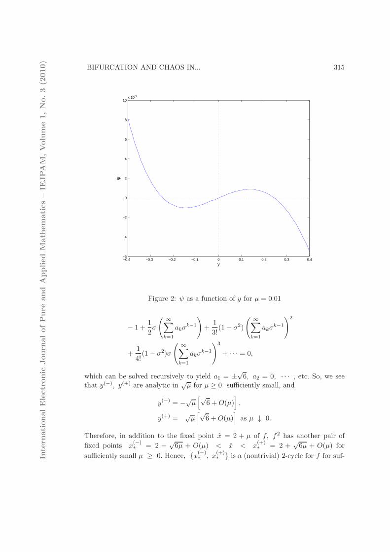
ψ(y) = ψ(y; µ) := 2(2 + µ) − [(2 + µ) + y][1 + e−y] = 0. (11)

Clearly y = 0 is a solution of (11) for every µ ≥ 0, and this corresponds to the fixedpoint x = x = a of f . But, there are two other solutions that comprise a (nontrivial)2-cycle of f . Noting that ψ(0; µ) = 0 for all µ ≥ 0, ψ → −∞ as y → +∞, ψ →+∞ as y → −∞, dψ

dy(0; µ) = µ, and performing a more detailed curve plotting

analysis, we find that graph of ψ has the form shown below for µ > 0. Accordinglyit has a positive and negative zero y(+) = y(+)(µ) and y(−) = y(−)(µ), respectively,for every sufficiently small positive value of the parameter µ. To find the nature ofthese zeros, we assume series solutions of the form

y(−) =

∞∑

k=1

a(−)k σk, y(+) =

∞∑

k=1

a(+)k σk,

where σ =√µ (µ ≥ 0). We then substitute these series in (11), wherein we use the

expansion e−y =∑∞

k=0(−1)kyk! , to obtain

ψ = 2(2 + σ2) − [(2 + σ2) + y][2 +

∞∑

k=1

(−1)kyk

k!] = 0,

− σ2 +σ2y

2+

1

3!(1 − σ2)y2 +

1

4!(1 − σ2)y3 + · · · = 0,

− σ2 +σ2

2σ

( ∞∑

k=1

akσk−1

)

+1

3!(1 − σ2)σ2

( ∞∑

k=1

akσk−1

)2

+1

4!(1 − σ2)σ2σ

( ∞∑

k=1

akσk−1

)3

+ · · · = 0,

Inte

rnati

onalEle

ctr

onic

Journ

alofP

ure

and

Applied

Math

em

ati

cs

–IE

JPA

M,V

olu

me

1,N

o.3

(2010)


−0.4 −0.3 −0.2 −0.1 0 0.1 0.2 0.3 0.4−6

−4

−2

0

2

4

6

8

10x 10

−3

y

ψ

Figure 2: ψ as a function of y for µ = 0.01

− 1 +1

2σ

( ∞∑

k=1

akσk−1

)

+1

3!(1 − σ2)

( ∞∑

k=1

akσk−1

)2

+1

4!(1 − σ2)σ

( ∞∑

k=1

akσk−1

)3

+ · · · = 0,

which can be solved recursively to yield a1 = ±√

6, a2 = 0, · · · , etc. So, we seethat y(−), y(+) are analytic in

√µ for µ ≥ 0 sufficiently small, and

y(−) = −√µ[√

6 +O(µ)]

,

y(+) =√µ[√

6 +O(µ)]

as µ ↓ 0.

Therefore, in addition to the fixed point x = 2 + µ of f, f2 has another pair of

fixed points x(−)∗ = 2 − √

6µ + O(µ) < x < x(+)∗ = 2 +

√6µ + O(µ) for

sufficiently small µ ≥ 0. Hence, {x(−)∗ , x

(+)∗ } is a (nontrivial) 2-cycle for f for suf-In

tern

ati

onalEle

ctr

onic

Journ

alofP

ure

and

Applied

Math

em

ati

cs

–IE

JPA

M,V

olu

me

1,N

o.3

(2010)


ficiently small positive µ, and this is stable since it is easy to verify that |f2′(x(−)∗ )| =

|f ′(x(−)∗ )f ′(x(+)

∗ )| < 1 for µ > 0 sufficiently small. Thus the proof is complete.

4.1. Codimension – One Flip Bifurcations

We now use the above results to show that if any of the parameters a, b or c varies,while the other two are fixed, the whole system exhibits a supercritical flip bifurca-tion. The dynamics of our discrete hierarchical system is determined by the iteratesof the map F : R3

+ → R3+ defined as

F (x) = F (x1, x2, x3) = (f1(x1; a), f2(x1, x2; b), f3(x1, x2, x3; c)), (12)

where f1, f2, f3 are either pioneer or climax type functions, and we have indicatedonly the dependence on the positive parameters a, b and since we are assuming thatonly they, and not the interaction coefficients cij are allowed to vary.

Recall that the derivative matrix of F at any point can be represented by thetriangular Jacobian matrix

F ′(x) =

∂f1∂x1

0 0∂f2∂x1

∂f2∂x2

0∂f3∂x1

∂f3∂x2

∂f3∂x3

(13)

with eigenvalues λ1 = ∂f1∂x1

(x), λ2 = ∂f2∂x2

(x), λ3 = ∂f3∂x3

(x) that may be viewedas associated with the parameters a, b and c respectively. Our codimension-onegeneralization of Theorem 4.4 is the following result, which is proved in Appendix.

Theorem 4.5. Let one of the three eigenvalues be equal to −1 and the othertwo eigenvalues be less than one in absolute value at a fixed point of F . Let v =a, b or c be the parameter associated with eigenvalue equal to −1. Then there is abifurcation value v∗ and corresponding fixed point x of F giving rise to a supercriticalflip bifurcation.

4.2. Codimension – Two Flip Bifurcations

Let us consider the case where two of the parameters a, b and c are varied – sayalong a curve in one of the parameter planes passing through a point where two ofthe eigenvalues of (13) are equal −1, while the remaining eigenvalue is of absolutevalue less than one. A natural question to ask for this codimension −2 parametervariation is, what are the properties of any flip bifurcations that may occur?

To see what flip possibilities there may be, it is instructive to first investigatethe simple, uncoupled all-pioneer map

P (x1, x2, x3) = (x1ea−x1 , x2e

b−x2 , x3ec−x3)In

tern

ati

onalEle

ctr

onic

Journ

alofP

ure

and

Applied

Math

em

ati

cs

–IE

JPA

M,V

olu

me

1,N

o.3

(2010)


with a = b = 2 and 0 < c < 2. Let us fix c and vary a and b along the curve b− a =0 in the a, b-plane, concentrating on a neighborhood of (a, b) = (2, 2) in thisplane. Owing to the fact that the system is uncoupled, Theorem 4.4 applied toeach coordinate function yields the following characterization of the flip bifurcationsat x∗ = (a = 2, b = 2, c): As a and b cross the value 2 in an increasing fashion alongany smooth curve in the a, b-plane passing through (2, 2), flip bifurcations occur.These bifurcations can be described as follows: In addition to the trivial, unstable2-cycle at (a, b, c) we have:

1. There are a pair of (nontrivial) stable 2-cycles; namely {(a+y(−)1 , b+y

(−)2 , c),

(a+ y(+)1 , b+ y

(+)2 , c)} and {(a+ y

(−)1 , b+ y

(+)2 , c), (a+ y

(+)1 , b+ y

(+)2 , c)}.

2. There are also two (nontrivial) stable 2-cycles; namely {(a+ y(−)1 , b, c), (a+

y(+)1 , b, c)} and {(a, b+ y

(−)2 , c), (a, b+ y

(−)1 , c)},

and in all cases the fixed point (a, b, c) changes from an attractor to a repeller uponsuch a crossing of (2, 2) in the a, b-plane.

As one might expect, our general hierarchical 3-dimensional system has analo-gous qualitative, codimension-2 flip bifurcation behavior. We summarize this in thefollowing theorem, which we prove in Appendix.

Theorem 4.6. Suppose that two of the eigenvalues of (13) at a fixed point x areequal to −1, while the remaining eigenvalue is less than one in absolute value. Letthe parameters associated with the eigenvalues equal to −1 be varied across a smoothcurve through the point in their coordinate plane so as to simultaneously increasethe two parameters. Then just as in the uncoupled case above, in a neighborhoodof the fixed point x, x changes from an attractor to a repeller as the parameterspass through the bifurcation point, giving birth to four (nontrivial) 2-cycles; two ofwhich are stable, while the other two are unstable.

4.3. Codimension – Three Flip Bifurcations

To complete our analysis of flip bifurcations, we consider the case where a, b and c aresimultaneously varied past values where all of the eigenvalues of (13) are equalto −1. Again we take our cue from the uncoupled, all pioneer system; this timewith a = b = c = 2, and a, b and c simultaneously exceeding 2 along some curvein a, b, c-space passing through (2, 2, 2). By analogy with our codimension-2 flipbifurcation investigation of (12), it is easy to see that for a = 2+µ1, b = 2+µ2 andc = 2+µ3 with µ1, µ2, µ3 ≥ 0 sufficiently small, we have the following flip bifurcationproperties: There are four stable 2-cycles; namely

{(a+ φ(+)(√µ1), b+ φ(+)(

√µ2), c+ φ(+)(

√µ3)),

(a+ φ(−)(√µ1), b+ φ(−)(

√µ2), c+ φ(−)(

√µ3))},In

tern

ati

onalEle

ctr

onic

Journ

alofP

ure

and

Applied

Math

em

ati

cs

–IE

JPA

M,V

olu

me

1,N

o.3

(2010)


{(a+ φ(+)(√µ1), b+ φ(+)(

√µ2), c+ φ(−)(

√µ3)),

(a+ φ(−)(√µ1), b+ φ(−)(

√µ2), c+ φ(+)(

√µ3))},

{(a+ φ(+)(√µ1), b+ φ(−)(

√µ2), c+ φ(+)(

√µ3)),

(a+ φ(−)(√µ1), b+ φ(+)(

√µ2), c+ φ(−)(

√µ3))},

and

{(a+ φ(+)(√µ1), b+ φ(−)(

√µ2), c+ φ(−)(

√µ3)),

(a+ φ(−)(√µ1), b+ φ(+)(

√µ2), c+ φ(+)(

√µ3))}.

Moreover, there are ten unstable 2-cycles, which are the fixed point (a, b, c) andthe nontrivial 2-cycles

{(a+ φ(+)(√µ1), b, c), (a+ φ(−)(

√µ1), b, c)},

{(a, b+ φ(+)(√µ2), c), (a, b+ φ(−)(

√µ2), c)},

{(a, b, c+ φ(+)(√µ3)), (a, b, c+ φ(−)(

√µ3))},

{(a+ φ(+)(√µ1), b+ φ(+)(

√µ2), c), (a+ φ(−)(

√µ1), b+ φ(−)(

√µ2), c)},

{(a+ φ(+)(√µ1), b+ φ(−)(

√µ2), c), (a+ φ(−)(

√µ1), b+ φ(+)(

√µ1), c)},

{(a+ φ(+)(√µ1), b, c+ φ(+)(

√µ3)), (a+ φ(−)(

√µ1), b, c+ φ(−)(

√µ3))},

{(a+ φ(+)(√µ1), b, c+ φ(−)(

√µ3)), (a+ φ(−)(

√µ1), b, c+ φ(+)(

√µ3))},

{(a, b+ φ(+)(√µ2), c+ φ(+)(

√µ3)), (a, b+ φ(−)(

√µ2), c+ φ(−)(

√µ3))},

{(a, b+ φ(+)(√µ2), c+ φ(−)(

√µ3)), (a, b+ φ(−)(

√µ2), c+ φ(+)(

√µ3))}.

In view of our analysis of codimension-2 flip bifurcations for our hierarchical map,it should come as no surprise that the qualitative behavior of the general case is thesame as for the uncoupled system. More precisely, we have the following result thatcan be proved using the same techniques as in the codimension-1 and codimension-2cases (albeit with many more detailed calculations), so that we omit the proof (cf.[9]).

Theorem 4.7. Suppose that all three of the eigenvalues of (13) are equal to-1 at a fixed point x of F for a particular set of parameter values (a, b, c) =(a0, b0, c0) and consider (a, b, c) = (a0, b0, c0) + (µ1, µ2, µ3) for sufficientlysmall µ1, µ2, µ3 ≥ 0, defining x = x(a, b, c) and x∗ = x(a, b, c)+(y1, y2, y3). Thenfor µ1, µ2, µ3 > 0 sufficiently small, F 2(x∗) = x∗ has 27 solutions comprising a totalof thirteen (non trivial) two-cycles of F near x(a0, b0, c0) and the fixed point. These2-cycles consist of four stable 2-cycles, and nine unstable 2-cycles; while the fixedpoint x is unstable. All of these 2-cycles depend analytically on (

√µ1,

√µ2,

√µ2) for

sufficiently small µ1, µ2, µ3 ≥ 0, and shrink to x(a0, b0, c0) as√µ1+

√µ2+

√µ3 ↓ 0.

Inte

rnati

onalEle

ctr

onic

Journ

alofP

ure

and

Applied

Math

em

ati

cs

–IE

JPA

M,V

olu

me

1,N

o.3

(2010)


5. Chaotic Dynamics

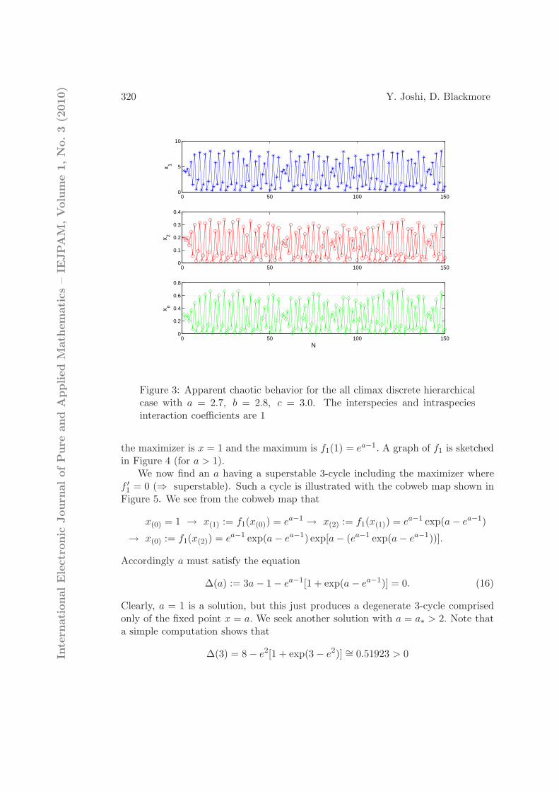
In this section we shall study chaotic regimes for our HPCM. Naturally, we shalltake advantage of the h-principle to reduce the analysis to a 1-dimensional mapin most cases, but we shall also have something to say about finding chaos in thecomplete higher dimensional system. “Perhaps” the most interesting behavior thatone may observe in population dynamics is transition to chaotic regimes, possiblyincluding strange chaotic attractors. From an ecologist’s point of view, chaos playsan important role in predicting (or more accurately not being able to make long-timepredictions about) the growth of plants in an ecosystem. If chaotic dynamics occurs,the behavior of the species can, besides being quite unpredictable to the point ofappearing stochastic, be extremely complex and especially interesting. It appearsfrom our simulations that our 3-dimensional all-climax discrete hierarchical modelcan exhibit chaotic dynamics, as shown in Figure 3 for the case where

F (x1, x2, x3) =(

x21e

2.7−x1 , x2(x1 + x2)e2.8−x1−x2, x3(x1 + x2 + x3)e

3−x1−x2−x3)

.(14)

5.1. Three-Cycle Induced Chaos

We now proceed to prove that the one-dimensional pioneer case has a 3-cycle, whichinduces chaos in the HPCM if it has a pioneer coordinate function in accordancewith the h-principle and [12], [21]. To demonstrate this, we consider the followingall-pioneer version of the HPCM

F (x1, x2, x3) = (f1(x1), f2(x1, x2), f3(x1, x2, x3))

:=(

x1ea−x1 , x2e

b−αx1−x2, x3ec−βx1−γx2−x3

)

, (15)

where a, b, c > 0 and α, β, γ > 0. We restrict our demonstration to showing howchaos in the first coordinate map induced by the existence of a superstable 3-cyclefor x → f1(x) := xea−x generates a chaotic orbit for the whole system. Note firstthat f1(0) = 0 and f1(x) ↓ 0 as x ↑ ∞. The fixed points are x = 0 and x = a. Tosee if these are stable, we compute

f ′1 = (1 − x)ea−x.

Hence,

f ′1(0) = ea > 1 ⇒ 0 is an unstable fixed point,

f ′1(a) = (1 − a) ⇒ x = a is stable if 0 < a < 2 and unstable if a > 2.

Let us find the maximum and maximizer for this function. As

f ′1 = (1 − x)ea−x = 0 ⇒ x = 1,Inte

rnati

onalEle

ctr

onic

Journ

alofP

ure

and

Applied

Math

em

ati

cs

–IE

JPA

M,V

olu

me

1,N

o.3

(2010)


0 50 100 1500

5

10

x 1

0 50 100 1500

0.1

0.2

0.3

0.4

x 2

0 50 100 1500

0.2

0.4

0.6

0.8

N

x n

Figure 3: Apparent chaotic behavior for the all climax discrete hierarchicalcase with a = 2.7, b = 2.8, c = 3.0. The interspecies and intraspeciesinteraction coefficients are 1

the maximizer is x = 1 and the maximum is f1(1) = ea−1. A graph of f1 is sketchedin Figure 4 (for a > 1).

We now find an a having a superstable 3-cycle including the maximizer wheref ′1 = 0 (⇒ superstable). Such a cycle is illustrated with the cobweb map shown inFigure 5. We see from the cobweb map that

x(0) = 1 → x(1) := f1(x(0)) = ea−1 → x(2) := f1(x(1)) = ea−1 exp(a− ea−1)

→ x(0) := f1(x(2)) = ea−1 exp(a− ea−1) exp[a− (ea−1 exp(a− ea−1))].

Accordingly a must satisfy the equation

∆(a) := 3a− 1 − ea−1[1 + exp(a− ea−1)] = 0. (16)

Clearly, a = 1 is a solution, but this just produces a degenerate 3-cycle comprisedonly of the fixed point x = a. We seek another solution with a = a∗ > 2. Note thata simple computation shows that

∆(3) = 8 − e2[1 + exp(3 − e2)] ∼= 0.51923 > 0Inte

rnati

onalEle

ctr

onic

Journ

alofP

ure

and

Applied

Math

em

ati

cs

–IE

JPA

M,V

olu

me

1,N

o.3

(2010)


0 1 2 3 4 50

0.5

1

1.5

2

2.5

3

3.5

4

4.5

5

x

f(x)

= x

ea−x

Figure 4: A cobweb map for pioneer species with the positive parameter a =1.8

and

∆(4) = 11 − e3[1 + exp(4 − e3)] ∼= −9.08554 < 0.

Thus the desired solution of (16) lies between 3 and 4. Using the bisection method[10], we compute that

a∗ ∼= 3.1167,

and conclude that f(x) := xea−x has a superstable 3-cycle comprised of the points{1, ea∗−1, ea∗−1 exp(a∗ − ea∗−1)}.

Returning to the original system (15), let us first consider the case where, α, β, γ =0, so we have the uncoupled system

x1(n+ 1) = x1(n)ea∗−x1(n),

x2(n+ 1) = x2(n)eb−x2(n), (17)

x3(n+ 1) = x3(n)ec−x3(n).

If we set b = c = 1.5, then it is clear from the above that

{(1, b, c), (ea∗−1, b, c), (ea∗−1 exp(a∗ − ea∗−1), b, c)}Inte

rnati

onalEle

ctr

onic

Journ

alofP

ure

and

Applied

Math

em

ati

cs

–IE

JPA

M,V

olu

me

1,N

o.3

(2010)


0 1 2 3 4 5 6 7 8 90

1

2

3

4

5

6

7

8

9

x

f(x)

= x

ea−x

(a) A superstable 3-cycle

0 0.5 1 1.5 20

0.5

1

1.5

2

x

f(x)

= x

ea−x

(b) Zoomed version of Figure 5(a)

Figure 5: Cobweb map for pioneer species with parameters a =3.1167 and c11 = 1

is a stable 3-cycle of (15). We want to consider some coupling, but not to the extentthat it perturbs this stable 3-cycle by much. Therefore, we consider the followingIn

tern

ati

onalEle

ctr

onic

Journ

alofP

ure

and

Applied

Math

em

ati

cs

–IE

JPA

M,V

olu

me

1,N

o.3

(2010)


special case:

x1(n+ 1) = x1(n)ea∗−x1(n),

x2(n+ 1) = x2(n)e1.5−0.3x1(n)−x2(n), (18)

x3(n+ 1) = x3(n)e1.5−0.3x1(n)−0.3x2(n)−x3(n).

It follows from the h-principle that this has a 3-cycle of the form

{(1, x(0)2 , x

(0)3 ), (ea∗−1, x

(1)2 , x

(1)3 ), (ea∗−1 exp(a∗ − ea∗−1), x

(2)2 , x

(2)3 )}.

A bit of straightforward analysis of the corresponding solution of F 3(x) = x (backed

up by numerical simulations) is all that it takes to show that we can choose x(0)2 and

x(0)3 close to b = c = 1.5 in a way that x

(1)2 , x

(1)3 , x

(2)2 and x

(2)3 are also close to 1.5,

and that the 3-cycle is stable. Of course, period three does not necessarily implychaos in more than one dimension, but we do obtain chaos since the 1-dimensionalfirst coordinate has a (superstable) 3-cycle. The difference between orbits startingnear (but not on) the 3-cycles of these two systems is that for (17) only the iterates ofthe x1 coordinate are chaotic, while in the case of (18) all of the coordinate iteratesevolve chaotically.

The existence of a chaotic orbit is additionally supported by the bifurcationdiagrams in Figs. 6 and 7 and computation of the Lyapunov exponent of an orbit forthe first coordinate map starting near x1 = 1 shown in Figure 8. These observationsand calculations also apply to the cases when the second and third coordinate mapshave chaotic orbits, and to a more general HPCM comprised of any permutation ofpioneer and climax coordinate maps.

5.2. Period-Doubling Route to Chaos

It follows from the h-principle that if any pioneer or climax coordinate map inour HPCM exhibits the well-known (for unimodal maps) period-doubling route tochaos, so does the entire system. The bifurcation diagrams in Figs. 6 and 7, andFigure 9 show the behavior of a pioneer and climax species, respectively, for a rangeof values of a. One sees the expected appearance of chaos beyond the limit of aperiod-doubling cascade in each case.

For the pioneer map f(x) = xea−x, as a increases from 0 we have a single stablefixed point at x = a. But at a ∼= 1.985, the fixed point becomes unstable andbifurcates into a stable 2-cycle comprising points just to the right and left of a via aflip bifurcation. This two-cycle further becomes unstable and bifurcates into a stable4-cycle and these period-doubling bifurcations continue with increasing a, generatinga period-doubling cascade that reaches a limit at a ∼= 2.69. There is a period-3window at a ∼= 3.105, showing the existence of chaos for a single species owing to thework of Sharkovski [21] and Li and Yorke [12]. Note that beyond a ∼= 8.575 it appearsIn

tern

ati

onalEle

ctr

onic

Journ

alofP

ure

and

Applied

Math

em

ati

cs

–IE

JPA

M,V

olu

me

1,N

o.3

(2010)


that the bifurcation diagram degenerates to zero, indicating an almost complete lackof stable invariant subsets. The Lyapunov exponent λ graph in Figure 8 confirmsthese observations, indicating the existence of chaotic orbits (since λ > 0) for mostvalues exceeding the period-doubling limit. We also see a very strong positive jumpin the exponent at a ∼= 7.67 followed by monotone increasing values, which we shallhave more to say about shortly.

In the case of a climax coordinate map g(x) = x2ea−x, there is an analogousperiod-doubling cascade leading to chaos depicted in the bifurcation diagram inFigure 9. However, in this case x = 0 remains superstable for all a, and there is apositive stable fixed point for 1 < a < 3 − ln 3. As a increases just beyond 3 − ln 3,the fixed point becomes unstable and gives birth to a stable 2-cycle, which becomesunstable at a ∼= 2.43 and generates a stable 4-cycle. This process continues andgenerates a period-doubling cascade with a limit of a ∼= 2.45, and one can expectthe existence of chaotic regimes beyond this parameter value. There is a period-3 window at a ∼= 2.62, which implies chaos for this 1-dimensional map (and theentire HPCM owing to the h-principle). The bifurcation diagram collapses to thesuperstable attractor at the origin for a ∼= 2.97, and it is not difficult to show (in factit follows directly from our shift map construction in the sequel) that the origin isan almost global attractor for a > 2.97, in the sense that it attracts all orbits exceptthose starting on a set of (Lebesgue) measure zero. The conclusions concerning theexistence of chaotic orbits for the climax map are also supported by the graph ofLyapunov exponents in Figure 10.

5.3. Shift Map Chaos

The existence of chaotic orbits for a climax map can also be proved using a fairlystandard construction that demonstrating that there is a compact invariant set onwhich g acts like a shift map (cf. [1], [5], [7], [15], [26]). Consider the 1-dimensionalclimax species map

g(x) := x2ea−x.

Numerical experiments indicate that we can apply the standard Cantor set argumentto prove existence of chaos when a ≥ 2.98, so we will now focus our attention on thespecific map

g(x) = x2e2.98−x (19)

having the graph shown in Figure 11. The fixed points of g are 0, and approxi-mately 0.0536 and 4.4795. An x ∈ I = [0.0536, 10.6436] has two types of orbits:one which directly or eventually goes to the origin (extinction or saturation of pop-ulation leading to extinction) and a second which does not converge to the origin(flourishing). We are interested in the second case. So, we shall remove all the subin-tervals from I which give rise to orbits converging to the origin and then observethe behavior of (19) on the remainder of I.In

tern

ati

onalEle

ctr

onic

Journ

alofP

ure

and

Applied

Math

em

ati

cs

–IE

JPA

M,V

olu

me

1,N

o.3

(2010)


Figure 6: Bifurcation diagram for a pioneer species. Here the parame-ter a varies from 0-4

Let us denote the set of all points in I whose iterates do not converge to the originby Λ. We clearly have the subinterval I0 = (1.54, 2.55) whose points ultimately go

to the origin. Next we have two more subintervals: I(−)1 = (0.32, 0.45) on the left

of I0 and I(+)1 = (5.42, 6.19) on the right of I0. They represent g−1(I0), the preimage

of I0. So the points in I(−)1 , I

(+)1 are first mapped to I0 and then they go to the origin.

We will remove these three subintervals from I. Now we repeat this procedure,

i.e. to find the preimage of I(−)1 which is I

(−)2 = (0.13, 0.16) ∪ (0.77, 0.86) and

of I(+)1 which is I

(+)2 = (3.85, 4.12)∪ (7.91, 8.36). At any stage k of this process, we

find 2k subintervals whose forward iterates under g converge to the origin, and areto be removed from I. This construction is illustrated in Figure 11.

This process of removal generates a compact, 2-component Cantor set (of mea-sure zero) defined as

Λ := I r

(

I0 ∪(

⋃∞k=1

I(±)k

))

.

It is clear from the construction that g(Λ) ⊂ Λ, so this Cantor set is invariant.Inte

rnati

onalEle

ctr

onic

Journ

alofP

ure

and

Applied

Math

em

ati

cs

–IE

JPA

M,V

olu

me

1,N

o.3

(2010)


Figure 7: Bifurcation diagram for a pioneer species. Here the parame-ter a varies from 4-10

Each x ∈ Λ can be identified with a binary sequence as follows:

x↔ .a0a1a2 . . .

where,

ak :=

{

0, gk(x) ∈ J0;1, gk(x) ∈ J1,

where J0 = [0.0536, 1.54) and J1 = (2.55, 10.6436]. The fixed points 0.0536 and 4.4795 naturally belong to J0 and J1, respectively, since the iterates of these points arefixed. In terms of the identification (homeomorphism), the positive fixed points areidentified with the points .0000 . . . and .1111 . . . respectively. Note here that thisalso shows that the set of initial points whose orbits do not converge to zero hasmeasure zero.

The restriction g|Λ is, by a standard argument (see, e.g. [1], [5], [15], [26]) thatfollows right from its definition, topologically conjugate to the shift map σ : S →S, defined in the space of binary sequences of the form .a0a1a2, . . . as

σ(.a0a1a2 . . .) := .a1a2a3 . . .Inte

rnati

onalEle

ctr

onic

Journ

alofP

ure

and

Applied

Math

em

ati

cs

–IE

JPA

M,V

olu

me

1,N

o.3

(2010)


0 1 2 3 4 5 6 7 8 9 10−35

−30

−25

−20

−15

−10

−5

0

5

10

a

λ

Figure 8: Lyapunov exponents for a pioneer species

Therefore, g is chaotic on Λ and has such features as periodic orbits of all periodsand a dense orbit. Accordingly the h-principle implies the existence of chaotic orbitsfor the HPCM with a climax coordinate function having a sufficiently large growthrate.

5.4. Small Scale Strange Attractor Like Pioneer Behavior

Let us look a little more closely at the dynamics of both pioneer and climax co-ordinate maps for larger growth rates. Denote the pioneer and climax maps byfa(x) := xea−x and ga(x) := x2ea−x respectively, where the subscript a is includedto emphasize the dependence on this parameter. We have already essentially takencare of this for ga: Figure 9 shows that for a > 2.97 the bifurcation diagram col-lapses to a thickened x-axis, and Figure 10 indicates the existence of chaotic orbits.But this follows from our discussion in the preceding subsection, where we showedthat for such parameter values gna (x) converges almost everywhere to the superstableattractor at the origin, and the complement Λ of this attraction set is an unstablecompact, invariant, 2-component Cantor set on which ga acts like a shift map.

The bifurcation diagrams Figs. 6 and 7 and Lyapunov exponent graph Figure8 for fa exhibit analogous behavior, except that this occurs for a > 8.575 and theIn

tern

ati

onalEle

ctr

onic

Journ

alofP

ure

and

Applied

Math

em

ati

cs

–IE

JPA

M,V

olu

me

1,N

o.3

(2010)


Figure 9: Bifurcation diagram for a climax species. Here the parame-ter a varies from 1.1-4

Lyapunov exponent appears to be quite a bit more positive for the pioneer map.For such large values of a, the fixed point at the origin is strongly repelling ratherthan contracting as in the case of ga. Consequently, in spite of the similarities in thebifurcation diagrams and Lyapunov exponent graphs for fa and ga, their dynamicscannot be the same. It remains only to characterize the large growth rate dynamicsfor the pioneer map. What we shall show is that given any small positive ǫ, theorbit of almost every point visits the interval Iǫ := [0, ǫ) infinitely often and this

interval contains an invariant Cantor set for some iterate fN(ǫ)a on which it behaves

like a shift map (i.e. fa is a subshift). Consequently, there is something akin to astrange attractor in any small neighborhood of the origin, except almost all orbitsonly come close to the “attractor” infinitely often instead of converging to it. Thismay explain the thickening of the unstable origin in the bifurcation diagram andrapid increase in the Lyapunov exponent for large values of a.

To verify this behavior, first recall that the maximum, ea−1, of fa occurs atx = 1, so fa (R+) = [0, ea−1]. The image of the right end point of this intervalis f2

a (1) = exp(

2a− 1 − ea−1)

. It follows by a simple calculation that given any0 < ǫ ≪ 1, f2

a (1) < ǫ whenever a > 1 + ln(

ln(ǫ−2))

and a ≥ 4. Now fix an aInte

rnati

onalEle

ctr

onic

Journ

alofP

ure

and

Applied

Math

em

ati

cs

–IE

JPA

M,V

olu

me

1,N

o.3

(2010)


1 1.5 2 2.5 3 3.5 4−6

−5

−4

−3

−2

−1

0

1

a

λ

Figure 10: Lyapunov exponents for a climax species

satisfying these inequalities, and note that a simple calculation shows for examplethat f2

a (1) < 1.0 × 10−6 when a > 8.575. Define

Θ(a) := {x ∈ R+ : fna (x) ∈ Iǫ for infinitely many nonnegative integers n} .

The set Θ(a) is fa-invariant by its very definition, and a straightforward modificationof the Cantor set construction for the climax map above along with some basicmeasure theoretic results can be used to show that its complement has measure zero.Observe that the complement of Θ(a), which we denote as Ξ(a), also is invariant.

It is easy to see, by decreasing ǫ if necessary, that we can choose N = N(ǫ) > 2so large that the (restricted) function ϕ := fN

a|Iǫ has the following properties: (1) It

is unimodal. (2) ϕ has just one maximizer xm > 0 on Iǫ at which ϕ is equal to ea−1

and for which ϕ′(x) is positive (negative) when 0 ≤ x < xm (xm < x < ǫ). (3) Ithas precisely two fixed points: one at zero and the other at xr, where xm < xr < ǫ.(4) xr < ϕ(xm) = ea−1. In all, the graph of ϕ is essentially a strongly horizontallycontracted version of the graph of fa on [0, ea−1]. These properties can readilybe seen to imply that there exists b and an open subinterval U of Iǫ such thatxr < b < ǫ, xm ∈ U and ϕ(U) ∩ [0, b] = ∅. In a manner analogous to that in theIn

tern

ati

onalEle

ctr

onic

Journ

alofP

ure

and

Applied

Math

em

ati

cs

–IE

JPA

M,V

olu

me

1,N

o.3

(2010)


0 2 4 6 8 10 120

2

4

6

8

10

12

x

f(x)

= x

2 e2.98

−x

I0

I1+

I2+

I

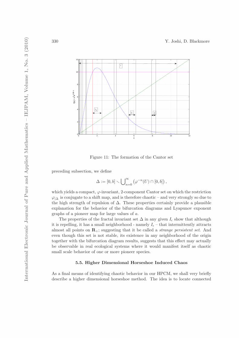
Figure 11: The formation of the Cantor set

preceding subsection, we define

∆ := [0, b] r

⋃∞n=0

(

ϕ−n(U) ∩ [0, b])

,

which yields a compact, ϕ-invariant, 2-component Cantor set on which the restrictionϕ|∆ is conjugate to a shift map, and is therefore chaotic – and very strongly so due tothe high strength of repulsion of ∆. These properties certainly provide a plausibleexplanation for the behavior of the bifurcation diagrams and Lyapunov exponentgraphs of a pioneer map for large values of a.

The properties of the fractal invariant set ∆ in any given Iǫ show that althoughit is repelling, it has a small neighborhood - namely Iǫ – that intermittently attractsalmost all points on R+; suggesting that it be called a strange persistent set. Andeven though this set is not stable, its existence in any neighborhood of the origintogether with the bifurcation diagram results, suggests that this effect may actuallybe observable in real ecological systems where it would manifest itself as chaoticsmall scale behavior of one or more pioneer species.

5.5. Higher Dimensional Horseshoe Induced Chaos

As a final means of identifying chaotic behavior in our HPCM, we shall very brieflydescribe a higher dimensional horseshoe method. The idea is to locate connectedIn

tern

ati

onalEle

ctr

onic

Journ

alofP

ure

and

Applied

Math

em

ati

cs

–IE

JPA

M,V

olu

me

1,N

o.3

(2010)


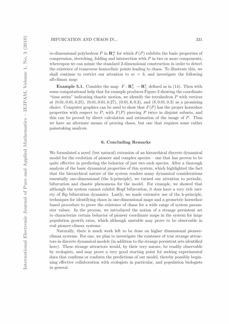
m-dimensional polyhedron P in Rm+ for which F (P ) exhibits the basic properties of

compression, stretching, folding and intersection with P in two or more components,whereupon we can mimic the standard 2-dimensional construction in order to detectthe existence of transverse homoclinic points leading to chaos. To illustrate this, weshall continue to restrict our attention to m = 3, and investigate the followingall-climax map:

Example 5.1. Consider the map F : R3+ → R3

+ defined as in (14). Then withsome computational help that for example produces Figure 3 showing the coordinate“time series” indicating chaotic motion, we identify the tetrahedron P with verticesat (0.01, 0.01, 0.25), (0.01, 0.01, 0.27), (0.01, 6, 0.3), and (8, 0.01, 0.3) as a promisingchoice. Computer graphics can be used to show that F (P ) has the proper horseshoeproperties with respect to P , with F (P ) piercing P twice in disjoint subsets, andthis can be proved by direct calculation and estimation of the image of P . Thuswe have an alternate means of proving chaos, but one that requires some ratherpainstaking analysis.

6. Concluding Remarks

We formulated a novel (but natural) extension of an hierarchical discrete dynamicalmodel for the evolution of pioneer and complex species – one that has proven to bequite effective in predicting the behavior of just two such species. After a thoroughanalysis of the basic dynamical properties of this system, which highlighted the factthat the hierarchical nature of the system renders many dynamical considerationsessentially one-dimensional (the h-principle), we turned our attention to periodic,bifurcation and chaotic phenomena for the model. For example, we showed thatalthough the system cannot exhibit Hopf bifurcation, it does have a very rich vari-ety of flip bifurcation dynamics. Lastly, we made extensive use of the h-principle,techniques for identifying chaos in one-dimensional maps and a geometric horseshoebased procedure to prove the existence of chaos for a wide range of system param-eter values. In the process, we introduced the notion of a strange persistent setto characterize certain behavior of pioneer coordinate maps in the system for largepopulation growth rates, which although unstable may prove to be observable inreal pioneer-climax systems.

Naturally, there is much work left to be done on higher dimensional pioneer-climax systems. For one, we plan to investigate the existence of true strange attrac-tors in discrete dynamical models (in addition to the strange persistent sets identifiedhere). These strange attractors would, by their very nature, be readily observableby ecologists, and may prove a very good starting point for seeking experimentaldata that confirms or confutes the predictions of our model, thereby possibly begin-ning effective collaboration with ecologists in particular, and population biologistsin general.In

tern

ati

onalEle

ctr

onic

Journ

alofP

ure

and

Applied

Math

em

ati

cs

–IE

JPA

M,V

olu

me

1,N

o.3

(2010)


Acknowledgments

A portion of this paper was taken from the dissertation of the first author, completedin partial fulfillment of the requirements for the degree of Doctor of Philosophy inthe Mathematical Sciences at the New Jersey Institute of Technology.

References

[1] D.K. Arrowsmith, C.M. Place, Dynamical Systems: Differential Equations,

Maps and Chaotic Behaviour, Chapman and Hall, London (1992).

[2] J. Best, C. Castillo-Chavez, A.-A. Yakubu, Hierarchical competition in discretetime models with dispersal, Fields Institute Communications, 36 (2004), 59-86.

[3] J.E. Franke, A.-A. Yakubu, Exclusion principle for density-dependent discretepioneer-climax models, J. Math. Anal. Appl., 187 (1994), 1019-1046.

[4] J.E. Franke, A.-A. Yakubu, Pioneer exclusion in a one-hump discrete pioneer-climax competitive system, J. Math. Biol., 32 (1994), 771-787.

[5] J. Guckenheimer, P. Holmes, Nonlinear Oscillations, Dynamical Systems and

Bifurcations of Vector Fields, Springer-Verlag, New York (1983).

[6] M.P. Hassell, M.N. Comins, Discrete time models for two-species competition,Theoret. Population Biol., 9 (1976), 202-221.

[7] M.W. Hirsch, S. Smale, R.L. Devaney, Differential Equations, Dynamical Sys-

tems, and an Introduction to Chaos, Elsevier Academic Press (2004).

[8] G. Jegan, G. Ramesh, K. Muthuchelian, Resprouting of Pioneer and ClimaxSpecies in the Pachakumachi Hills, Cumbum Valley, Western Ghats, India,Ethnobotanical Leaflets, 12 (2008), 343-347.

[9] Y. Joshi, Discrete Dynamical Population Models: Higher Dimensional Pioneer-

Climax Models, Ph.D. Thesis, New Jersey Institute of Technology (2009).

[10] A. Kendall, Introduction to Numerical Analysis, Wiley, New York (1989).

[11] M.V. Kuijk, Forest Regeneration and Restoration in Vietnam, Ph.D. Thesis,Utrecht University (2008).

[12] Y.T. Li, J.A. Yorke, Period three implies chaos, Am. Math. Month., 82 (1975),985-992.Inte

rnati

onalEle

ctr

onic

Journ

alofP

ure

and

Applied

Math

em

ati

cs

–IE

JPA

M,V

olu

me

1,N

o.3

(2010)


[13] D. Raaimakers, R.G.A. Boot, R. Dijkstra, S. Pot, T. Pons, Photosyntheticrates in relation to leaf phosphorus content in pioneer versus climax tropicalrainforest trees, Oecologia, 12 (1995), 120-125.

[14] D. Raaimakers, H. Lambers, Response to phosphorus supply of tropical treeseedlings: a comparison between a pioneer species Tapirira obtusa and a climaxspecies Lecythis corrugata, Netv PhytoL, 132 (1996), 97-102.

[15] C. Robinson, Dynamical Systems: Stability, Symbolic Dynamics, and Chaos,CRC Press Inc., Boca Raton (1995).

[16] J.F. Selgrade, Planting and harvesting for pioneer-climax models, Rocky Moun-

tain J. Math., 24 (1994), 293-310.

[17] J.F. Selgrade, G. Namkoong, Stable periodic behavior in a pioneer-climaxmodel, Nat. Resour. Model, 4 (1990), 215-227.

[18] J.F. Selgrade, G. Namkoong, Population interactions with growth rates depen-dent on weighted densities, Differential Equation Models in Biology, Epidemi-

ology and Ecology, Lecture Notes in Biomath., 92 (1991), 247-256.

[19] J.F. Selgrade, J.H. Roberds, Lumped-density population models of pioneer-climax type and stability analysis of Hopf bifurcations, Math. Biosci., 135

(1996), 1-21.

[20] J.F. Selgrade, J.H. Roberds, Period-doubling bifurcations for systems of differ-ence equations and applications to models in population biology, Nonlin. Anal.:

Theory, Methods and Applications, 29 (1997), 185-199.

[21] A.N. Sharkovski, Co-existence of the cycles of a continuous mapping of the lineinto itself, Ukrainian Math. Z., 16 (1964), 61-71.

[22] M. Silvestrini, I.F.M. Valio, E.A. de. Mattos, Photosynthesis and carbon gainunder contrasting light levels in seedlings of a pioneer and a climax tree from aBrazilian semideciduous tropical forest, Rev. Bras. Bot., 30 (2007), 463-474.

[23] S. Sumner, Dynamical Systems Associated with Pioneer-Climax Models, Ph.D.Thesis, North Carolina State University (1992).

[24] S. Sumner, Hopf bifurcation in pioneer-climax competing species models, Math.

Biosci., 137 (1996), 1-24.

[25] Wikipedia, Lambert W function — Wikipedia, The Free Encyclopedia (2009),http://en.wikipedia.org/w/index.php?title=Lambert W function&oldid=306160Inte

rnati

onalEle

ctr

onic

Journ

alofP

ure

and

Applied

Math

em

ati

cs

–IE

JPA

M,V

olu

me

1,N

o.3

(2010)


[26] S. Wiggins, Introduction to Applied Nonlinear Dynamical Systems and Chaos,Springer, New York (2003).

A. Appendix

We now give detailed proofs of Theorems 4.5 and 4.6.

A.1. Proof of Theorem on Codimension-1 Flip Bifurcations

For simplicity, we consider only the all-pioneer case, noting that all other combina-tions of pioneer and climax coordinate functions (with other interaction coefficients)can be dealt with analogously:

F (x) = (f1(x1; a), f2(x1, x2; b), f3(x1, x2, x3; c))

= (x1ea−x1 , x2e

b−x1−x2, x3ec−x1−x2−x3). (20)

The fixed point in question must be x = (a, b− a, c− b). If it is λ1 that equals −1,with associated v = a, the proof follows directly from the one-dimensional result inTheorem 4.4. If λ2 = −1, or λ3 = −1 with associated parameters b or c, respectively,the proof – in keeping with the h-principle – is only slightly more difficult. Weconsider only λ2 = −1, since the proof for λ3 = −1 is virtually the same. In thiscase, we see from (20) that the eigenvalues of F ′(x) are −1 < λ1 = 1 − a < 1, λ2 =1 − (b − a) = −1 and −1 < λ3 = 1 − (c − b) < 1. Now we fix a and vary b slightlywhile keeping c fixed and maintaining −1 < 1 − (c− b) < 1. Observe that

F 2(x) = F (F (x))

= (f1(f1(x1)), f2(f1(x1), f2(x1, x2)), f3(f1(x1), f2(x1, x2), f3(x1, x2, x3)))

= (x1 exp[2a− x1(1 + ea−x1)], x2 exp[2b− x1(1 + ea−x1) − x2(1 + eb−x1−x2)],

x3 exp[2c − x1(1 + ea−x1) − x2(1 + eb−x1−x2) − x3(1 + ec−x1−x2−x3)]) (21)

and it is easy to see that F 2(x) = F 2(a, b − a, c − b) = x, so naturally x is alsoa fixed point of F 2. To find the bifurcation in the x2 coordinate, we set v = b =a+ 2 + µ = v∗ + µ, x2 = (b− a) + y2 = 2 + µ+ y2 and x3 = c− b+ y3. We want tofind fixed points x∗ = x + (0, y2, y3) of F 2 near x for sufficiently small µ ≥ 0. Itfollows from (21) that x∗ must satisfy the equations

2(2 + µ) − (2 + µ+ y2)(1 + e−y2) = 0,

2(c− a) − (b− a+ y2)(1 + e−y2) − (c− b+ y3)(1 + e−y2−y3) = 0. (22)

We see from the proof of Theorem 4.4 that the first of the above equations has in

addition to y2 = 0 a pair of nonzero solutions y(−)2 = −√

µ[√

6+O(µ)] ≤ 0 ≤ y(+)2 =In

tern

ati

onalEle

ctr

onic

Journ

alofP

ure

and

Applied

Math

em

ati

cs

–IE

JPA

M,V

olu

me

1,N

o.3

(2010)


√µ[√

6 +O(µ)] for all sufficiently small µ ≥ 0. Upon substituting either of these inthe second of equations (22), and taking note of the first equation, we obtain

ψ(y3, µ) := 2(c − b) − (c− b+ y3)(1 + e−y(±)2 (

√µ)−y3) = 0.

We compute that dψdy3

(0, µ) = −1 + [(c − b) − 1]e−y(±)2 (

√µ), whereupon it follows

from −1 < λ3 = 1 − (c − b) < 1 that this derivative is not zero for all sufficientlysmall µ. Hence, we infer from the implicit function theorem that (22) has a unique

solution y(±)3 = y

(±)3 (µ) going to zero with µ, and y3(µ) is actually a smooth function

of y2(µ), which is a smooth function of√µ. Collecting all of the above properties,

we see that

x(+)∗ = (a, b− a+ y

(+)2 , c− b+ y

(+)3 ),

x(−)∗ = F (x

(+)∗ ) = (a, b− a+ y

(−)2 , c− b+ y

(−)3 )

is a 2-cycle of F in a neighborhood of the fixed point x = (a, b − a, c − b) for b =a+2+µ varying and the parameters a and c fixed. In addition, it is straightforward

to show that ||x−x∗|| = O(√µ) and that the eigenvalues of F 2′(x(−)

∗ ) = eigenvalues

of F 2′(x(+)∗ ) all have absolute value less than 1, so {x∗, F (x∗)} is a stable 2-cycle. As

it is clear that the fixed point x∗ is unstable (in the x2 direction) for all sufficientlysmall µ > 0, the proof is complete.

A.2. Proof of Theorem on Codimension-2 Flip Bifurcations

Once again, we shall give the proof only for the all-pioneer system (20), and here weshall only consider the case where λ1 = 1 − a = λ2 = 1 − (b − a) = −1, and −1 <λ3 = 1 − (c − b) < 1. A proof for the most general case, which we leave to thereader can be based on the argument that follows, with only minor modifications.We simply extend the methods of proof of Theorems 4.4 and 4.5. Denote the fixedpoint of F as x := (a, b − a, c − b), and set a = 2 + µ and b = a + 2 + ν =4 + µ + ν, where µ, ν ≥ 0 are sufficiently small. Define x∗ = x + (y1, y2, y3) =(2 + µ+ ν, 2 + ν + y2, c− (4 + µ+ ν) + y3), which denotes solutions of F 2(x∗) =x∗ for µ, ν ≥ 0 sufficiently small, and the y1, y2, y3 are correspondingly smallcoordinate increments. Extending the arguments in the proofs of Theorems 4.4and 4.5 in the obvious ways, it is easy to see that the increments must satisfy thefollowing system of equations:

2(2 + µ) − [(2 + µ) + y1][1 + e−y1] = 0,

2(4 + µ+ ν) − [(2 + µ) + y1][1 + e−y1] − [(2 + ν) + y2][1 + e−y1−y2] = 0,

2c− [(2 + µ)y1][1 + e−y1] − [(2 + ν) + y2][1 + e−y1−y2]

−[(c− 4 − µ− ν) + y3][1 + e−y1−y2−y3] = 0. (23)

Inte

rnati

onalEle

ctr

onic

Journ

alofP

ure

and

Applied

Math

em

ati

cs

–IE

JPA

M,V

olu

me

1,N

o.3

(2010)


Evidently y1 = y2 = y3 = 0 is a solution of (23) for all µ, ν ≥ 0, and this correspondsto x, which is a fixed point of F and therefore trivially a fixed point of F 2. It remainsto find the nontrivial fixed points of F 2 near x, which generate nontrivial 2-cyclesof F for sufficiently small µ, ν ≥ 0. We infer from Theorem 4.4 that along with y1 =

0, there is pair of solutions y(±)1 = φ(±)(

√µ) = ±√

6µ+O(µ), where φ(±) are analyticfunctions for sufficiently small µ ≥ 0. We now proceed to the second of equations(23) for each of y1 = 0, φ(−)(

√µ) and φ(+)(

√µ). Substituting y1 = 0 in the second

equation of (23) yields

2(2 + ν) − [(2 + ν) + y2][1 + e−y2 ] = 0. (24)

Noting the similarity of (24) to the first equation of (23), it is clear that for y1 =0, the second equation of (23) has solutions y2 = 0 and y2 = φ(±)(

√ν) for all

sufficiently small nonnegative ν. On the other hand, substituting y1 = φ(±)(√µ) in

the second equation of (23) and using the fact that φ(±)(√µ) are solutions of the

first of equations (23), we readily compute that

2(2 + ν) − [(2 + ν) + y2][1 + e−φ(±)(

√µ)−y2 ] = 0.

Then again applying our approach in the proof of Theorem 4.4, we find that for each

of φ(−)(√µ) and φ(+)(

√µ) there are three solutions; namely, y2 = η

(−)(+)(

√µ,

√ν),

η(0)(+)(

√µ,

√ν), η

(+)(+)(

√µ,

√ν) for y1 = φ(+)(

√µ) and y2 = η

(−)(−)(

√µ,

√ν),

η(0)(−)(

√µ,

√ν), η

(+)(−)(

√µ,

√ν) for y1 = φ(−)(

√µ). These solutions satisfy the fol-

lowing readily verified properties: all of the functions are analytic for sufficientlysmall µ, ν ≥ 0,

η(−)(−)(

√µ,

√ν) < φ(−)(

√ν) < η

(−)(+)(

√µ,

√ν) < η

(0)(−)(

√µ,

√ν) < 0

< η(0)(+)(

√µ,

√ν) < η

(+)(+)(

√µ,

√ν) < φ(+)(

√ν) < η

(+)(−)(

√µ,

√ν), (25)

for all sufficiently small µ, ν > 0, and η(0, ±)(±) = O(

√µ,

√ν) as µ, ν ↓ 0. To

summarize our analysis so far, we have found that the first two equations of (23)have the following nine solutions for sufficiently small nonnegative values of theparameters µ and ν: (i) y1 = y2 = 0; (ii) y1 = 0, y2 = φ(+)(

√ν); (iii) y1 =

0, y2 = φ(−)(√ν); (iv) y1 = φ(+)(

√µ), y2 = η

(0)(+)(

√µ,

√ν); (v) y1 = φ(+)(

√µ), y2 =

η(+)(+)(

√µ,

√ν); (vi) y1 = φ(+)(

√µ), y2 = η

(−)(+)(

√µ,

√ν); (vii) y1 = φ(−)(

√µ), y2 =

η(0)(−)(

√µ,

√ν); (viii) y1 = φ(−)(

√µ), y2 = η

(+)(−)(

√µ,

√ν); and (ix) y1 = φ(−)(

√µ),

y2 = η(−)(−)(

√µ,

√ν). It remains to solve the last equation of (23), where each of

these nine solutions for the first two variables is substituted; this yields

ψ(y3; µ, ν) := 2(c− b) − [(c − b) + y3][1 + e−y1(√µ,

√ν)−y2(

√µ,

√ν)−y3 ] = 0 (26)In

tern

ati

onalEle

ctr

onic

Journ

alofP

ure

and

Applied

Math

em

ati

cs

–IE

JPA

M,V

olu

me

1,N

o.3

(2010)


where y1 = y1(√µ,

√ν), y2 = y2(

√µ,

√ν) are known analytic functions of (

√µ,

√ν)

for sufficiently small µ, ν ≥ 0 given in turn by each of the solutions (i)-(ix) of thefirst two equations. Now it follows from our assumption, |1 − (c− b)| < 1, that thesame is true for all sufficiently small µ, ν ≥ 0 in (26), which implies that

dψ

dy3(0; µ, ν) 6= 0,

and this completes the proof.

Inte

rnati

onalEle

ctr

onic

Journ

alofP

ure

and

Applied

Math

em

ati

cs

–IE

JPA

M,V

olu

me

1,N

o.3

(2010)

338

International Electronic Journal of Pure and Applied Mathematics – IEJPAM, Volume 1, No. 3 (2010)

my referred paper

Documents