mycsvtu notes() experiment no....
TRANSCRIPT
R.C.E.T. Bhilai/ Department of Computer Science and Engineering / DBMS Laboratory
1
MYcsvtu Notes(www.mycsvtunotes.in)
Experiment No. 1
Aim: Introduction to SQL
Description:
A Brief History of SQL
The history of SQL begins in an IBM laboratory in San Jose, California, where SQL was developed in the
late 1970s. The initials stand for Structured Query Language, and the language itself is often referred to as
"sequel." It was originally developed for IBM's DB2 product (a relational database management system, or
RDBMS, that can still be bought today for various platforms and environments). In fact, SQL makes an
RDBMS possible. SQL is a nonprocedural language, in contrast to the procedural or third-generation
languages (3GLs) such as COBOL and C that had been created up to that time.
The characteristic that differentiates a DBMS from an RDBMS is that the RDBMS provides a set-oriented
database language. For most RDBMSs, this set-oriented database language is SQL. Set oriented means that
SQL processes sets of data in groups.
Two standards organizations, the American National Standards Institute (ANSI) and the International
Standards Organization (ISO), currently promote SQL standards to industry. The ANSI-92 standard is the
standard for the SQL used throughout this book. Although these standard-making bodies prepare standards
for database system designers to follow, all database products differ from the ANSI standard to some
degree. In addition, most systems provide some proprietary extensions to SQL that extend the language into
a true procedural language. We have used various RDBMSs to prepare the examples in this book to give
you an idea of what to expect from the common database systems.
Dr. Codd's 12 Rules for a Relational Database Model
The most popular data storage model is the relational database, which grew from the seminal paper "A
Relational Model of Data for Large Shared Data Banks," written by Dr. E. F. Codd in 1970. SQL evolved to
service the concepts of the relational database model. Dr. Codd defined 13 rules, oddly enough referred to as
Codd's 12 Rules, for the relational model:
0. A relational DBMS must be able to manage databases entirely through its relational capabilities.
1. Information rule-- All information in a relational database (including table and column names) is
represented explicitly as values in tables.
2. Guaranteed access--Every value in a relational database is guaranteed to be accessible by using a
combination of the table name, primary key value, and column name.
3. Systematic null value support--The DBMS provides systematic support for the treatment of null values
(unknown or inapplicable data), distinct from default values, and independent of any domain.
R.C.E.T. Bhilai/ Department of Computer Science and Engineering / DBMS Laboratory
2
4. Active, online relational catalog--The description of the database and its contents is represented at the
logical level as tables and can therefore be queried using the database language.
5. Comprehensive data sublanguage--At least one supported language must have a well-defined syntax and
be comprehensive. It must support data definition, manipulation, integrity rules, authorization, and
transactions.
6. View updating rule--All views that are theoretically updatable can be updated through the system.
7. Set-level insertion, update, and deletion--The DBMS supports not only set-level retrievals but also set-
level inserts, updates, and deletes.
8. Physical data independence--Application programs and ad hoc programs are logically unaffected when
physical access methods or storage structures are altered.
9. Logical data independence--Application programs and ad hoc programs are logically unaffected, to the
extent possible, when changes are made to the table structures.
10. Integrity independence--The database language must be capable of defining integrity rules. They must
be stored in the online catalog, and they cannot be bypassed.
11. Distribution independence--Application programs and ad hoc requests are logically unaffected when
data is first distributed or when it is redistributed.
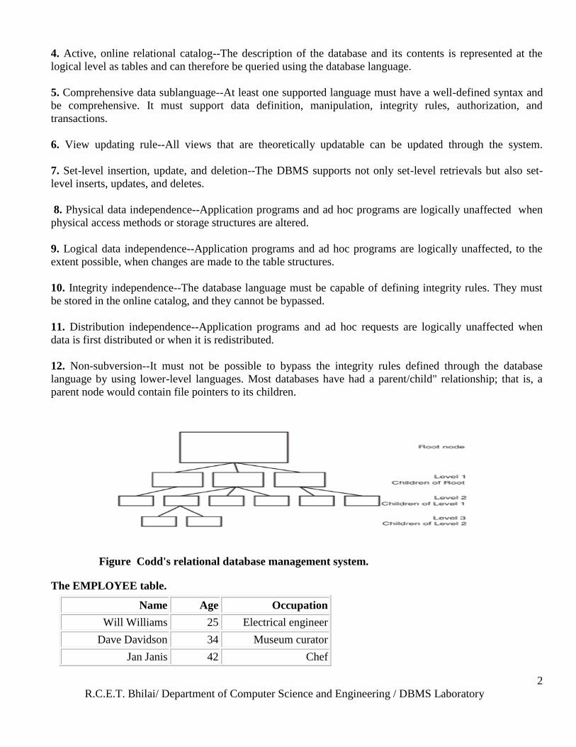
12. Non-subversion--It must not be possible to bypass the integrity rules defined through the database
language by using lower-level languages. Most databases have had a parent/child" relationship; that is, a
parent node would contain file pointers to its children.
Figure Codd's relational database management system.
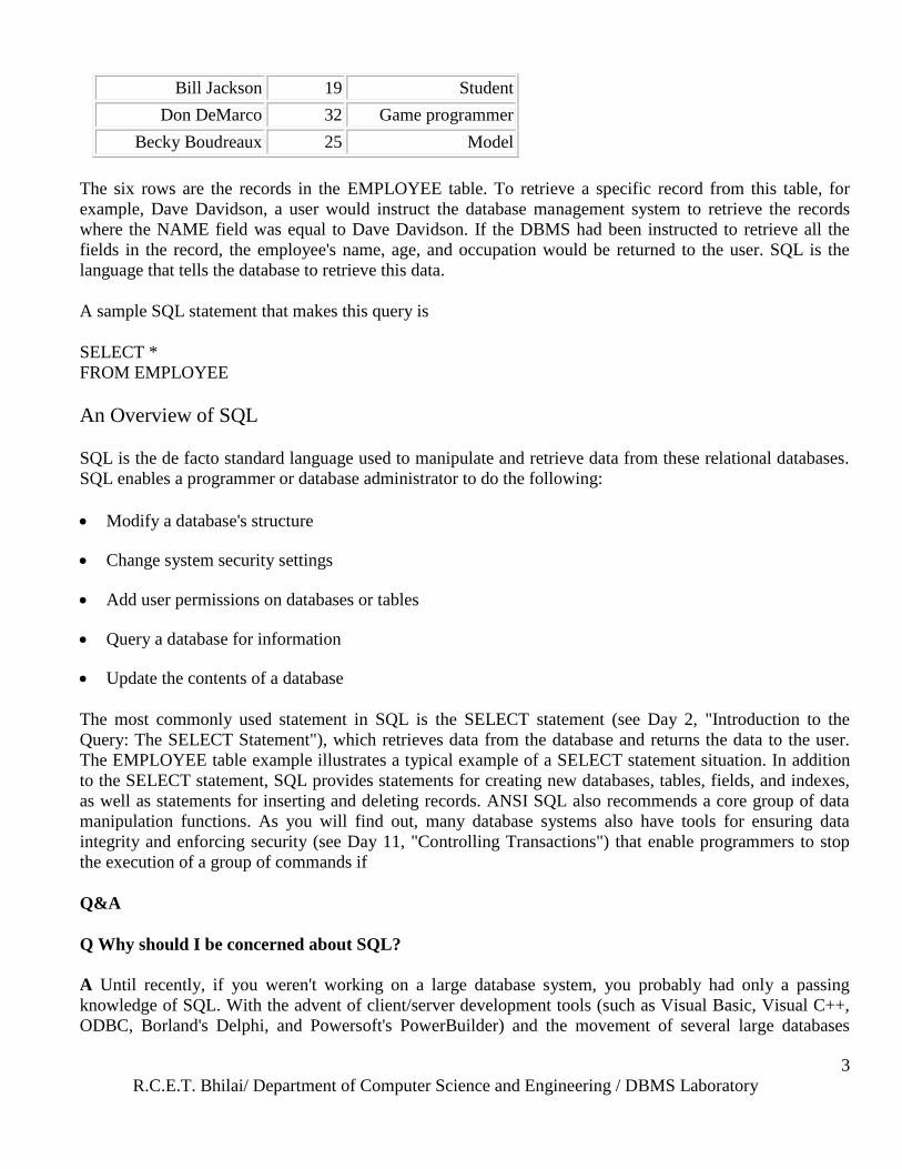
The EMPLOYEE table.
Name Age Occupation
Will Williams 25 Electrical engineer
Dave Davidson 34 Museum curator
Jan Janis 42 Chef
R.C.E.T. Bhilai/ Department of Computer Science and Engineering / DBMS Laboratory
3
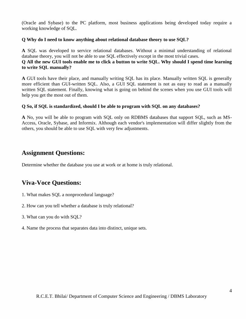
Bill Jackson 19 Student
Don DeMarco 32 Game programmer
Becky Boudreaux 25 Model
The six rows are the records in the EMPLOYEE table. To retrieve a specific record from this table, for
example, Dave Davidson, a user would instruct the database management system to retrieve the records
where the NAME field was equal to Dave Davidson. If the DBMS had been instructed to retrieve all the
fields in the record, the employee's name, age, and occupation would be returned to the user. SQL is the
language that tells the database to retrieve this data.
A sample SQL statement that makes this query is
SELECT *
FROM EMPLOYEE
An Overview of SQL
SQL is the de facto standard language used to manipulate and retrieve data from these relational databases.
SQL enables a programmer or database administrator to do the following:
Modify a database's structure
Change system security settings
Add user permissions on databases or tables
Query a database for information
Update the contents of a database
The most commonly used statement in SQL is the SELECT statement (see Day 2, "Introduction to the
Query: The SELECT Statement"), which retrieves data from the database and returns the data to the user.
The EMPLOYEE table example illustrates a typical example of a SELECT statement situation. In addition
to the SELECT statement, SQL provides statements for creating new databases, tables, fields, and indexes,
as well as statements for inserting and deleting records. ANSI SQL also recommends a core group of data
manipulation functions. As you will find out, many database systems also have tools for ensuring data
integrity and enforcing security (see Day 11, "Controlling Transactions") that enable programmers to stop
the execution of a group of commands if
Q&A
Q Why should I be concerned about SQL?
A Until recently, if you weren't working on a large database system, you probably had only a passing
knowledge of SQL. With the advent of client/server development tools (such as Visual Basic, Visual C++,
ODBC, Borland's Delphi, and Powersoft's PowerBuilder) and the movement of several large databases
R.C.E.T. Bhilai/ Department of Computer Science and Engineering / DBMS Laboratory
4
(Oracle and Sybase) to the PC platform, most business applications being developed today require a
working knowledge of SQL.
Q Why do I need to know anything about relational database theory to use SQL?
A SQL was developed to service relational databases. Without a minimal understanding of relational
database theory, you will not be able to use SQL effectively except in the most trivial cases.
Q All the new GUI tools enable me to click a button to write SQL. Why should I spend time learning
to write SQL manually?
A GUI tools have their place, and manually writing SQL has its place. Manually written SQL is generally
more efficient than GUI-written SQL. Also, a GUI SQL statement is not as easy to read as a manually
written SQL statement. Finally, knowing what is going on behind the scenes when you use GUI tools will
help you get the most out of them.
Q So, if SQL is standardized, should I be able to program with SQL on any databases?
A No, you will be able to program with SQL only on RDBMS databases that support SQL, such as MS-
Access, Oracle, Sybase, and Informix. Although each vendor's implementation will differ slightly from the
others, you should be able to use SQL with very few adjustments.
Assignment Questions:
Determine whether the database you use at work or at home is truly relational.
Viva-Voce Questions:
1. What makes SQL a nonprocedural language?
2. How can you tell whether a database is truly relational?
3. What can you do with SQL?
4. Name the process that separates data into distinct, unique sets.
R.C.E.T. Bhilai/ Department of Computer Science and Engineering / DBMS Laboratory
5
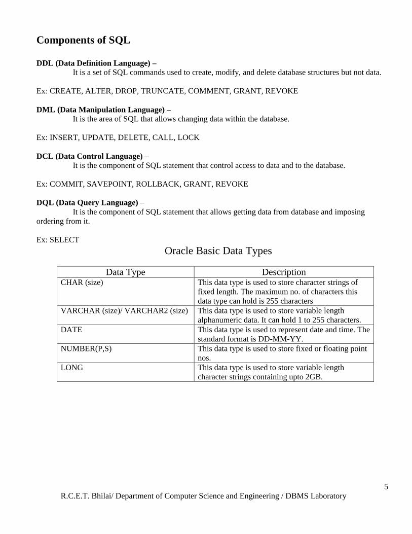
Components of SQL
DDL (Data Definition Language) –
It is a set of SQL commands used to create, modify, and delete database structures but not data.
Ex: CREATE, ALTER, DROP, TRUNCATE, COMMENT, GRANT, REVOKE
DML (Data Manipulation Language) – It is the area of SQL that allows changing data within the database.
Ex: INSERT, UPDATE, DELETE, CALL, LOCK
DCL (Data Control Language) – It is the component of SQL statement that control access to data and to the database.
Ex: COMMIT, SAVEPOINT, ROLLBACK, GRANT, REVOKE
DQL (Data Query Language) –
It is the component of SQL statement that allows getting data from database and imposing
ordering from it.
Ex: SELECT
Oracle Basic Data Types
Data Type Description CHAR (size)
This data type is used to store character strings of
fixed length. The maximum no. of characters this
data type can hold is 255 characters
VARCHAR (size)/ VARCHAR2 (size)
This data type is used to store variable length
alphanumeric data. It can hold 1 to 255 characters.
DATE
This data type is used to represent date and time. The
standard format is DD-MM-YY.
NUMBER(P,S)
This data type is used to store fixed or floating point
nos.
LONG
This data type is used to store variable length
character strings containing upto 2GB.
R.C.E.T. Bhilai/ Department of Computer Science and Engineering / DBMS Laboratory
6
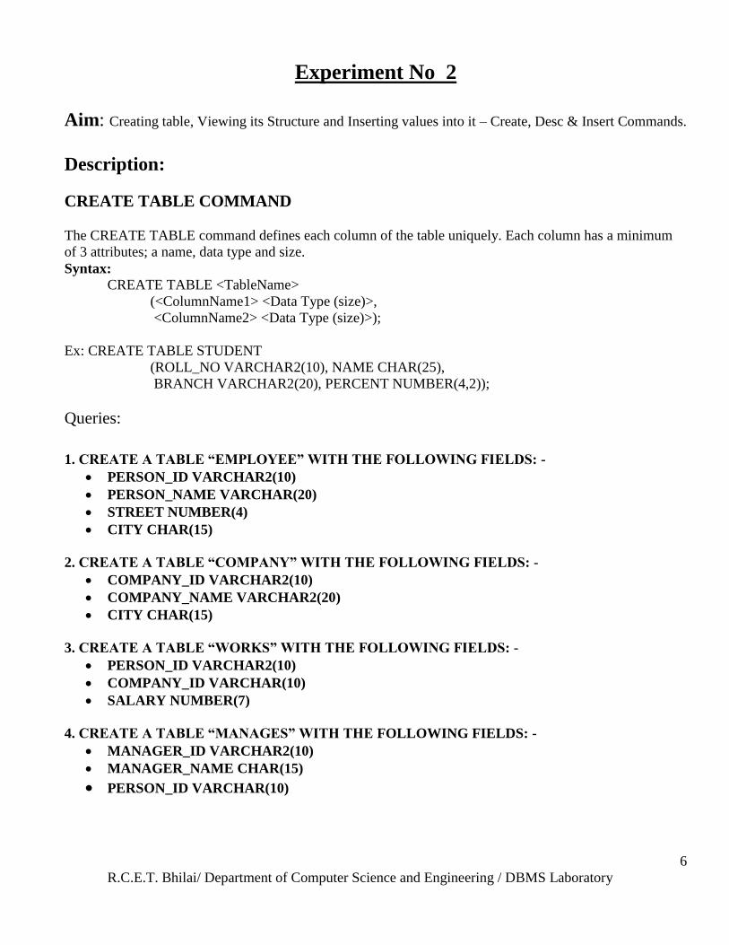
Experiment No 2
Aim: Creating table, Viewing its Structure and Inserting values into it – Create, Desc & Insert Commands.
Description:
CREATE TABLE COMMAND
The CREATE TABLE command defines each column of the table uniquely. Each column has a minimum
of 3 attributes; a name, data type and size.
Syntax:
CREATE TABLE <TableName>
(<ColumnName1> <Data Type (size)>,
<ColumnName2> <Data Type (size)>);
Ex: CREATE TABLE STUDENT
(ROLL_NO VARCHAR2(10), NAME CHAR(25),
BRANCH VARCHAR2(20), PERCENT NUMBER(4,2));
Queries:
1. CREATE A TABLE “EMPLOYEE” WITH THE FOLLOWING FIELDS: -
PERSON_ID VARCHAR2(10)
PERSON_NAME VARCHAR(20)
STREET NUMBER(4)
CITY CHAR(15)
2. CREATE A TABLE “COMPANY” WITH THE FOLLOWING FIELDS: -
COMPANY_ID VARCHAR2(10)
COMPANY_NAME VARCHAR2(20)
CITY CHAR(15)
3. CREATE A TABLE “WORKS” WITH THE FOLLOWING FIELDS: -
PERSON_ID VARCHAR2(10)
COMPANY_ID VARCHAR(10)
SALARY NUMBER(7)
4. CREATE A TABLE “MANAGES” WITH THE FOLLOWING FIELDS: -
MANAGER_ID VARCHAR2(10)
MANAGER_NAME CHAR(15)
PERSON_ID VARCHAR(10)
R.C.E.T. Bhilai/ Department of Computer Science and Engineering / DBMS Laboratory
7
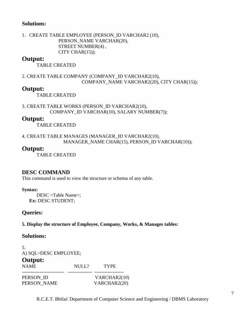
Solutions:
1. CREATE TABLE EMPLOYEE (PERSON_ID VARCHAR2 (10),
PERSON_NAME VARCHAR(20),
STREET NUMBER(4) ,
CITY CHAR(15));
Output: TABLE CREATED
2. CREATE TABLE COMPANY (COMPANY_ID VARCHAR2(10),
COMPANY_NAME VARCHAR2(20), CITY CHAR(15));
Output: TABLE CREATED
3. CREATE TABLE WORKS (PERSON_ID VARCHAR2(10),
COMPANY_ID VARCHAR(10), SALARY NUMBER(7));
Output: TABLE CREATED
4. CREATE TABLE MANAGES (MANAGER_ID VARCHAR2(10),
MANAGER_NAME CHAR(15), PERSON_ID VARCHAR(10));
Output: TABLE CREATED
DESC COMMAND
This command is used to view the structure or schema of any table.
Syntax:
DESC <Table Name>;
Ex: DESC STUDENT;
Queries:
5. Display the structure of Employee, Company, Works, & Manages tables:
Solutions:
5.
A) SQL>DESC EMPLOYEE;
Output: NAME NULL? TYPE
-------------------------- --------------- ------------------
PERSON_ID VARCHAR2(10)
PERSON_NAME VARCHAR2(20)
R.C.E.T. Bhilai/ Department of Computer Science and Engineering / DBMS Laboratory
8
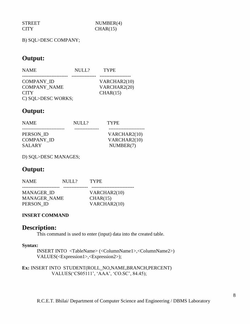
STREET NUMBER(4)
CITY CHAR(15)
B) SQL>DESC COMPANY;
Output:
NAME NULL? TYPE
---------------------------- --------------- -------------------
COMPANY_ID VARCHAR2(10)
COMPANY_NAME VARCHAR2(20)
CITY CHAR(15)
C) SQL>DESC WORKS;
Output:
NAME NULL? TYPE
-------------------------- --------------- ----------------------
PERSON_ID VARCHAR2(10)
COMPANY_ID VARCHAR2(10)
SALARY NUMBER(7)
D) SQL>DESC MANAGES;
Output:
NAME NULL? TYPE
----------------------- --------------- --------------------------
MANAGER_ID VARCHAR2(10)
MANAGER_NAME CHAR(15)
PERSON_ID VARCHAR2(10)
INSERT COMMAND
Description: This command is used to enter (input) data into the created table.
Syntax:
INSERT INTO <TableName> (<ColumnName1>,<ColumnName2>)
VALUES(<Expression1>,<Expression2>);
Ex: INSERT INTO STUDENT(ROLL_NO,NAME,BRANCH,PERCENT)
VALUES(‗CS05111‘, ‗AAA‘, ‗CO.SC‘, 84.45);
R.C.E.T. Bhilai/ Department of Computer Science and Engineering / DBMS Laboratory
9
Queries:
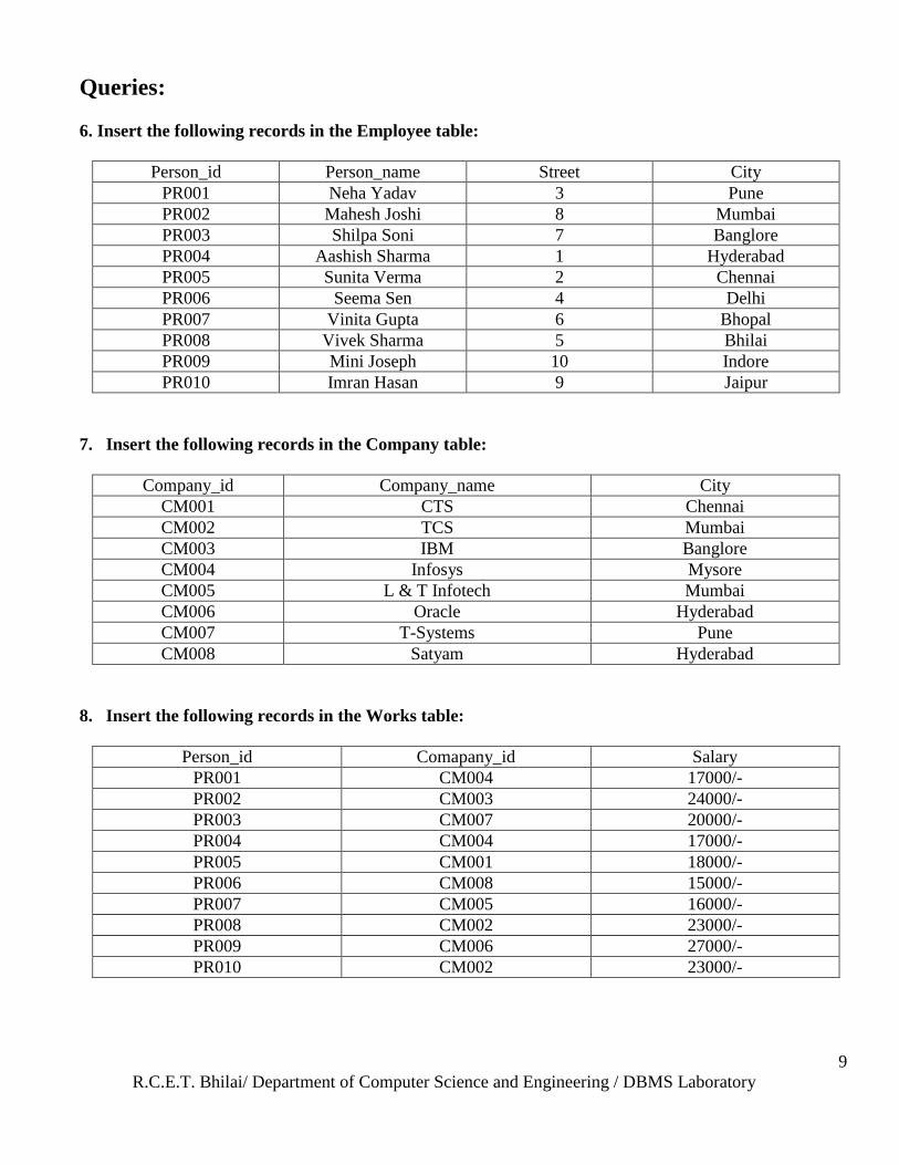
6. Insert the following records in the Employee table:
Person_id Person_name Street City
PR001 Neha Yadav 3 Pune
PR002 Mahesh Joshi 8 Mumbai
PR003 Shilpa Soni 7 Banglore
PR004 Aashish Sharma 1 Hyderabad
PR005 Sunita Verma 2 Chennai
PR006 Seema Sen 4 Delhi
PR007 Vinita Gupta 6 Bhopal
PR008 Vivek Sharma 5 Bhilai
PR009 Mini Joseph 10 Indore
PR010 Imran Hasan 9 Jaipur
7. Insert the following records in the Company table:
Company_id Company_name City
CM001 CTS Chennai
CM002 TCS Mumbai
CM003 IBM Banglore
CM004 Infosys Mysore
CM005 L & T Infotech Mumbai
CM006 Oracle Hyderabad
CM007 T-Systems Pune
CM008 Satyam Hyderabad
8. Insert the following records in the Works table:
Person_id Comapany_id Salary
PR001 CM004 17000/-
PR002 CM003 24000/-
PR003 CM007 20000/-
PR004 CM004 17000/-
PR005 CM001 18000/-
PR006 CM008 15000/-
PR007 CM005 16000/-
PR008 CM002 23000/-
PR009 CM006 27000/-
PR010 CM002 23000/-
R.C.E.T. Bhilai/ Department of Computer Science and Engineering / DBMS Laboratory
10
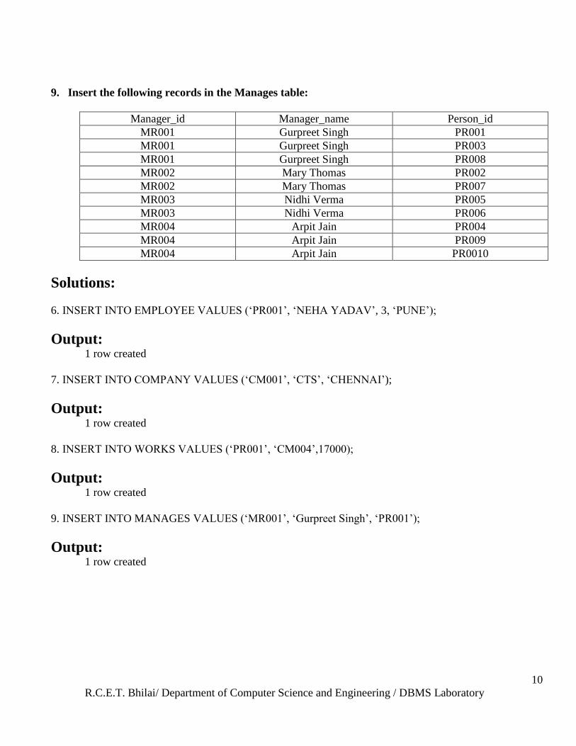
9. Insert the following records in the Manages table:
Manager_id Manager_name Person_id
MR001 Gurpreet Singh PR001
MR001 Gurpreet Singh PR003
MR001 Gurpreet Singh PR008
MR002 Mary Thomas PR002
MR002 Mary Thomas PR007
MR003 Nidhi Verma PR005
MR003 Nidhi Verma PR006
MR004 Arpit Jain PR004
MR004 Arpit Jain PR009
MR004 Arpit Jain PR0010
Solutions:
6. INSERT INTO EMPLOYEE VALUES (‗PR001‘, ‗NEHA YADAV‘, 3, ‗PUNE‘);
Output: 1 row created
7. INSERT INTO COMPANY VALUES (‗CM001‘, ‗CTS‘, ‗CHENNAI‘);
Output: 1 row created
8. INSERT INTO WORKS VALUES (‗PR001‘, ‗CM004‘,17000);
Output: 1 row created
9. INSERT INTO MANAGES VALUES (‗MR001‘, ‗Gurpreet Singh‘, ‗PR001‘);
Output: 1 row created
R.C.E.T. Bhilai/ Department of Computer Science and Engineering / DBMS Laboratory
11
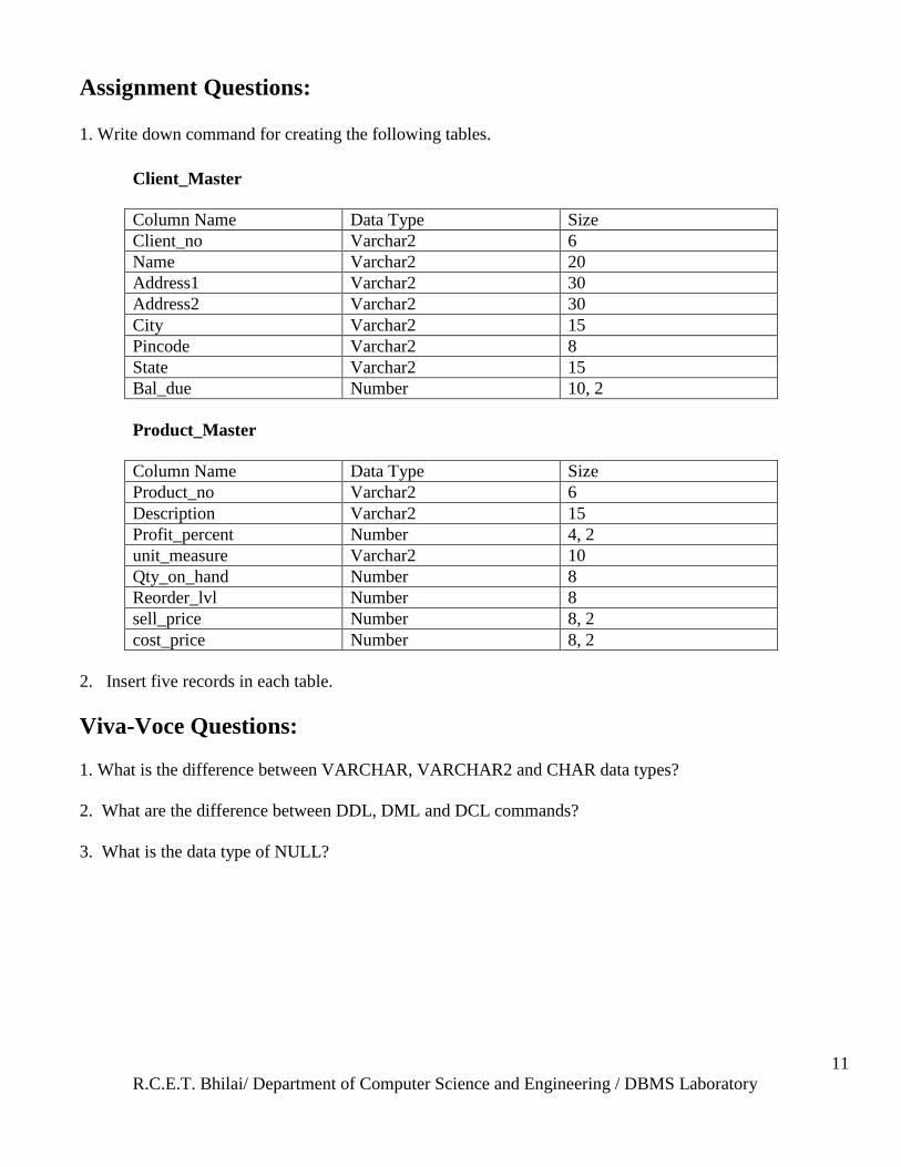
Assignment Questions: 1. Write down command for creating the following tables.
Client_Master
Column Name Data Type Size
Client_no Varchar2 6
Name Varchar2 20
Address1 Varchar2 30
Address2 Varchar2 30
City Varchar2 15
Pincode Varchar2 8
State Varchar2 15
Bal_due Number 10, 2
Product_Master
Column Name Data Type Size
Product_no Varchar2 6
Description Varchar2 15
Profit_percent Number 4, 2
unit_measure Varchar2 10
Qty_on_hand Number 8
Reorder_lvl Number 8
sell_price Number 8, 2
cost_price Number 8, 2
2. Insert five records in each table.
Viva-Voce Questions:
1. What is the difference between VARCHAR, VARCHAR2 and CHAR data types?
2. What are the difference between DDL, DML and DCL commands?
3. What is the data type of NULL?

R.C.E.T. Bhilai/ Department of Computer Science and Engineering / DBMS Laboratory
12
Experiment No 3
Aim: Viewing data from the tables, creating a table from a table – Select Command, As Select Clause.
Description:
WHERE CLAUSE This clause is used to specify any condition within a SQL statement.
Ex:
WHERE clause can be used with CREATE, SELECT, DELETE & UPDATE commands.
VIEWING DATA FROM THE TABLES
All Rows & Columns of a Table-
SELECT * FROM <Table Name>;
Ex: SELECT * FROM STUDENT;
Selected Columns & All Rows –
SELECT <Column Name1>, <Column Name2> FROM <Table Name>;
Ex: SELECT NAME, ROLL_NO FROM STUDENT;
Selected Rows & All Columns –
SELECT * FROM <TableName> WHERE <Condition>;
Ex: SELECT * FROM STUDENT WHERE NAME=‗AAA‘;
Queries:
10. Retrieve the entire contents of employee table.
11. Find out the names of all employees.
12. Find out the names of all companies.
13. Find out the names & cities of all companies.
14. List out names of all employees of „Bhilai‟ city.
15. List out names of all companies located in „Hyderabad‟.
R.C.E.T. Bhilai/ Department of Computer Science and Engineering / DBMS Laboratory
13
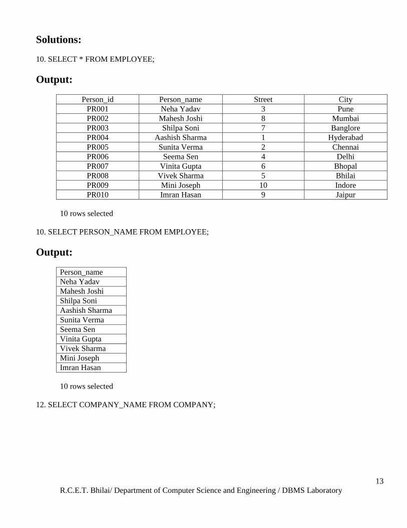
Solutions:
10. SELECT * FROM EMPLOYEE;
Output:
Person_id Person_name Street City
PR001 Neha Yadav 3 Pune
PR002 Mahesh Joshi 8 Mumbai
PR003 Shilpa Soni 7 Banglore
PR004 Aashish Sharma 1 Hyderabad
PR005 Sunita Verma 2 Chennai
PR006 Seema Sen 4 Delhi
PR007 Vinita Gupta 6 Bhopal
PR008 Vivek Sharma 5 Bhilai
PR009 Mini Joseph 10 Indore
PR010 Imran Hasan 9 Jaipur
10 rows selected
10. SELECT PERSON_NAME FROM EMPLOYEE;
Output:
Person_name
Neha Yadav
Mahesh Joshi
Shilpa Soni
Aashish Sharma
Sunita Verma
Seema Sen
Vinita Gupta
Vivek Sharma
Mini Joseph
Imran Hasan
10 rows selected
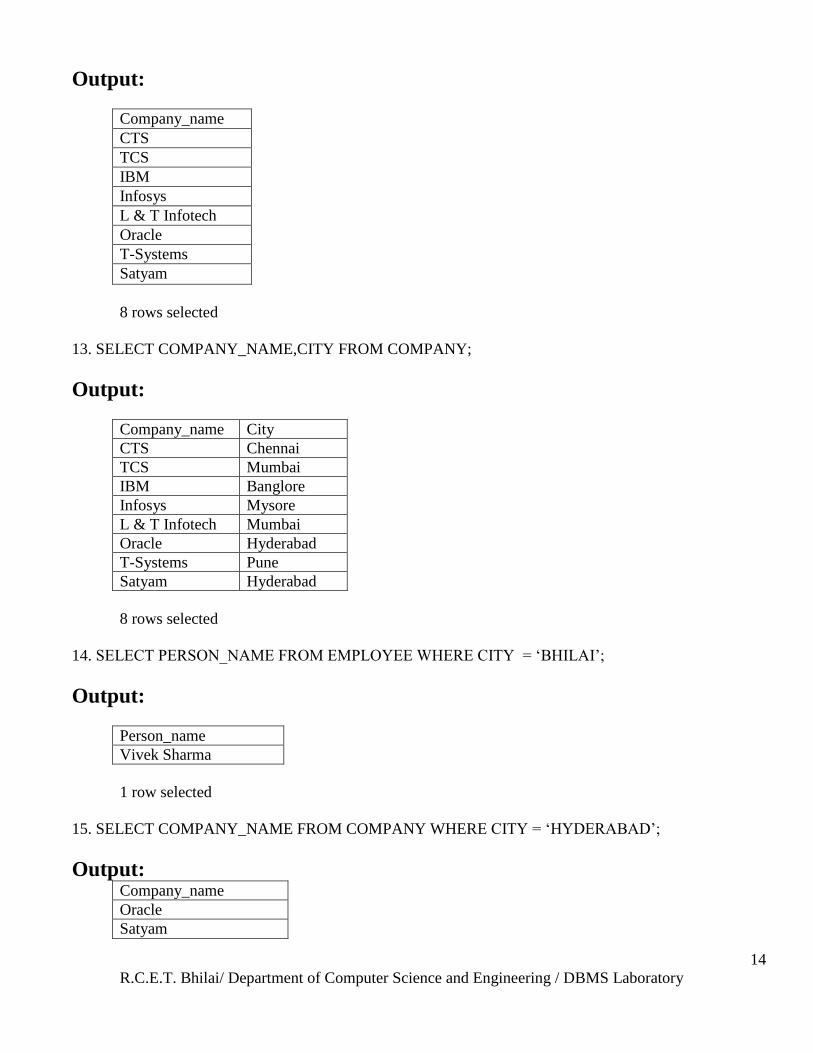
12. SELECT COMPANY_NAME FROM COMPANY;
R.C.E.T. Bhilai/ Department of Computer Science and Engineering / DBMS Laboratory
14
Output:
Company_name
CTS
TCS
IBM
Infosys
L & T Infotech
Oracle
T-Systems
Satyam
8 rows selected
13. SELECT COMPANY_NAME,CITY FROM COMPANY;
Output:
Company_name City
CTS Chennai
TCS Mumbai
IBM Banglore
Infosys Mysore
L & T Infotech Mumbai
Oracle Hyderabad
T-Systems Pune
Satyam Hyderabad
8 rows selected
14. SELECT PERSON_NAME FROM EMPLOYEE WHERE CITY = ‗BHILAI‘;
Output:
Person_name
Vivek Sharma
1 row selected
15. SELECT COMPANY_NAME FROM COMPANY WHERE CITY = ‗HYDERABAD‘;
Output: Company_name
Oracle
Satyam
R.C.E.T. Bhilai/ Department of Computer Science and Engineering / DBMS Laboratory
15
2 rows selected
ELIMINATING DUPLICATE ROWS WHEN USING A SELECT STATEMENT
Syntax:
SELECT DISTINCT <Column Name1>, <Column Name2>
FROM <Table Name>;
Ex: SELECT DISTINCT NAME, PERCENT FROM STUDENT;
Syntax:
SELECT DISTINCT * FROM <TableName>;
Ex: SELECT DISTINCT * FROM STUDENT;
Queries:
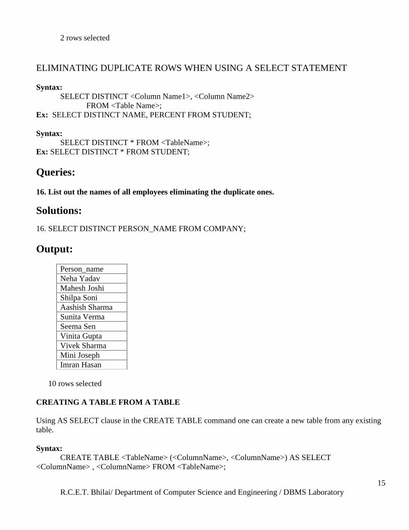
16. List out the names of all employees eliminating the duplicate ones.
Solutions:
16. SELECT DISTINCT PERSON_NAME FROM COMPANY;
Output:
10 rows selected
CREATING A TABLE FROM A TABLE
Using AS SELECT clause in the CREATE TABLE command one can create a new table from any existing
table.
Syntax:
CREATE TABLE <TableName> (<ColumnName>, <ColumnName>) AS SELECT
<ColumnName> , <ColumnName> FROM <TableName>;
Person_name
Neha Yadav
Mahesh Joshi
Shilpa Soni
Aashish Sharma
Sunita Verma
Seema Sen
Vinita Gupta
Vivek Sharma
Mini Joseph
Imran Hasan
R.C.E.T. Bhilai/ Department of Computer Science and Engineering / DBMS Laboratory
16
Ex:
CREATE TABLE GRADE (ROLL_NO, NAME, MARKS)
AS SELECT ROLL_NO, NAME, PERCENT FROM STUDENT;
Queries:
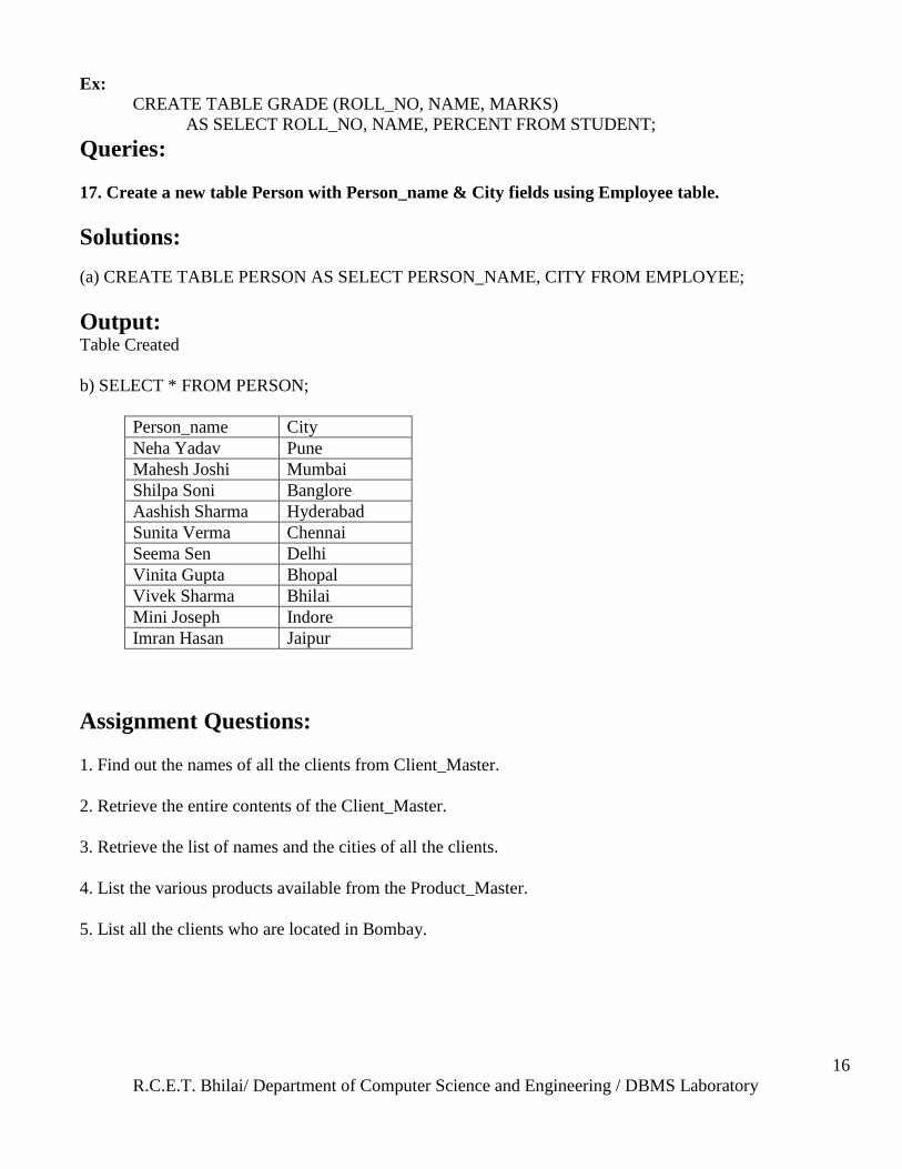
17. Create a new table Person with Person_name & City fields using Employee table.
Solutions:
(a) CREATE TABLE PERSON AS SELECT PERSON_NAME, CITY FROM EMPLOYEE;
Output: Table Created
b) SELECT * FROM PERSON;
Person_name City
Neha Yadav Pune
Mahesh Joshi Mumbai
Shilpa Soni Banglore
Aashish Sharma Hyderabad
Sunita Verma Chennai
Seema Sen Delhi
Vinita Gupta Bhopal
Vivek Sharma Bhilai
Mini Joseph Indore
Imran Hasan Jaipur
Assignment Questions:
1. Find out the names of all the clients from Client_Master.
2. Retrieve the entire contents of the Client_Master.
3. Retrieve the list of names and the cities of all the clients.
4. List the various products available from the Product_Master.
5. List all the clients who are located in Bombay.
R.C.E.T. Bhilai/ Department of Computer Science and Engineering / DBMS Laboratory
17
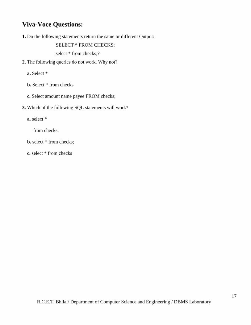
Viva-Voce Questions:
1. Do the following statements return the same or different Output:
SELECT * FROM CHECKS;
select * from checks;?
2. The following queries do not work. Why not?
a. Select *
b. Select * from checks
c. Select amount name payee FROM checks;
3. Which of the following SQL statements will work?
a. select *
from checks;
b. select * from checks;
c. select * from checks
R.C.E.T. Bhilai/ Department of Computer Science and Engineering / DBMS Laboratory
18
Experiment No 4
Aim: Sorting table data, removing rows from table, modifying rows of the table – Order By Clause,
Delete Command, Update Command
Description:
SORTING DATA IN A TABLE The rows retrieved from the table will be sorted in either ascending or descending order.
Syntax:
SELECT * FROM <TableName> ORDER BY <ColumnName1>,<ColumnName2>
<[SORT ORDER]>;
Ex:
i) SELECT * FROM STUDENT ORDER BY ROLL_NO, NAME;
ii) SELECT * FROM STUDENT ORDER BY NAME DESC;
Queries:
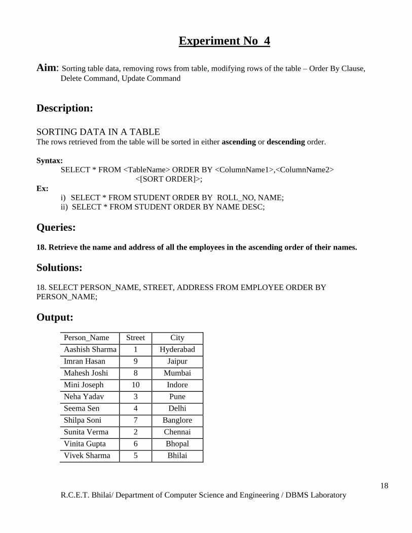
18. Retrieve the name and address of all the employees in the ascending order of their names.
Solutions:
18. SELECT PERSON_NAME, STREET, ADDRESS FROM EMPLOYEE ORDER BY
PERSON_NAME;
Output:
Person_Name Street City
Aashish Sharma 1 Hyderabad
Imran Hasan 9 Jaipur
Mahesh Joshi 8 Mumbai
Mini Joseph 10 Indore
Neha Yadav 3 Pune
Seema Sen 4 Delhi
Shilpa Soni 7 Banglore
Sunita Verma 2 Chennai
Vinita Gupta 6 Bhopal
Vivek Sharma 5 Bhilai
R.C.E.T. Bhilai/ Department of Computer Science and Engineering / DBMS Laboratory
19
DELETE OPERATION
Removal of All Rows:
DELETE FROM <TableName>;
Ex: DELETE FROM MARKS;
Removal of Specific Rows:
DELETE FROM <TableName> WHERE <Condition>;
Ex: DELETE FROM STUDENT WHERE NAME=‗PQR‘;
Queries:
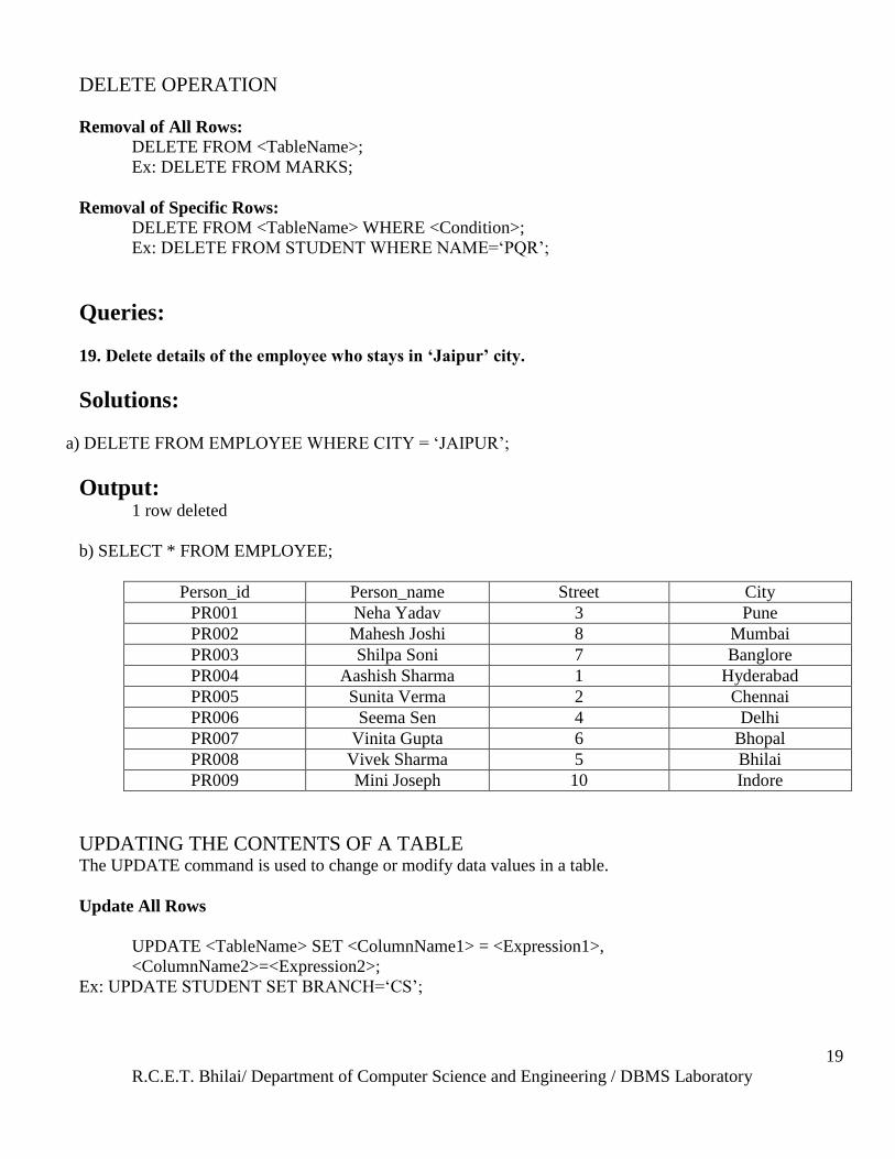
19. Delete details of the employee who stays in „Jaipur‟ city.
Solutions:
a) DELETE FROM EMPLOYEE WHERE CITY = ‗JAIPUR‘;
Output: 1 row deleted
b) SELECT * FROM EMPLOYEE;
Person_id Person_name Street City
PR001 Neha Yadav 3 Pune
PR002 Mahesh Joshi 8 Mumbai
PR003 Shilpa Soni 7 Banglore
PR004 Aashish Sharma 1 Hyderabad
PR005 Sunita Verma 2 Chennai
PR006 Seema Sen 4 Delhi
PR007 Vinita Gupta 6 Bhopal
PR008 Vivek Sharma 5 Bhilai
PR009 Mini Joseph 10 Indore
UPDATING THE CONTENTS OF A TABLE The UPDATE command is used to change or modify data values in a table.
Update All Rows
UPDATE <TableName> SET <ColumnName1> = <Expression1>,
<ColumnName2>=<Expression2>;
Ex: UPDATE STUDENT SET BRANCH=‗CS‘;
R.C.E.T. Bhilai/ Department of Computer Science and Engineering / DBMS Laboratory
20
Update Selected Rows
UPDATE <TableName> SET <ColumnName1> = <Expression1>,
<ColumnName2>=<Expression2> WHERE <Condition>
Ex: UPDATE STUDENT SET PERCENT = 81.25 WHERE ROLL_NO=‗CS/05/119‘;
Queries:
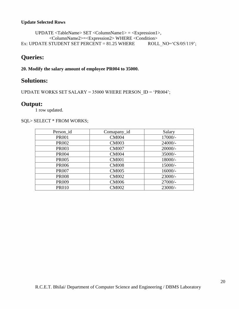
20. Modify the salary amount of employee PR004 to 35000.
Solutions:
UPDATE WORKS SET SALARY = 35000 WHERE PERSON_ID = ‗PR004‘;
Output: 1 row updated.
SQL> SELECT * FROM WORKS;
Person_id Comapany_id Salary
PR001 CM004 17000/-
PR002 CM003 24000/-
PR003 CM007 20000/-
PR004 CM004 35000/-
PR005 CM001 18000/-
PR006 CM008 15000/-
PR007 CM005 16000/-
PR008 CM002 23000/-
PR009 CM006 27000/-
PR010 CM002 23000/-
R.C.E.T. Bhilai/ Department of Computer Science and Engineering / DBMS Laboratory
21
Assignment Questions:
1. Change the city of client_no ‗C00005‘ to Bombay.
2. Change the bal_due of client_no ‗C00001‘ to Rs. 1000.
3. Delete all the products from Product_Master where the quantity on hand is equal to 100.
4. Delete from Client_Master where the column state holds the value ‗Tamil Nadu‘.
5. Display client names in alphabetical order from Client_Master.
Viva-Voce Questions:
1. Which clause allows data from a table to be viewed in a sorted order.
2. The ___________ command is used to change or modify data values in a table.
3. What is wrong with the following statement?
UPDATE COLLECTION ("HONUS WAGNER CARD", 25000, "FOUND IT");
4. What would happen if you issued the following statement?
SQL> DELETE * FROM COLLECTION;
R.C.E.T. Bhilai/ Department of Computer Science and Engineering / DBMS Laboratory
22
Experiment No 5
Aim: Modifying the structure of tables, Renaming tables, dropping table structure – Alter Table, Rename,
Drop, Truncate Command
Description:
MODIFYING THE STRUCTURE OF TABLES
The structure of a table can be modified by using the ALTER TABLE it is possible to add or delete
columns, create or destroy indexes, change the data of existing columns or rename columns or the table
itself.
Adding New Columns:
This command is used to add anew column at the end of the structure of an existing table.
Syntax: ALTER TABLE <TableName> ADD(<NewColumnName> <Datatype>(<size>),
<NewColumnName> <Datatype>(<size>),…….);
Ex: ALTER TABLE STUDENT ADD(AGE NUMBER(2));
Dropping a Column from the Table
This is used for removing a column of any existing table.
Syntax: ALTER TABLE <TableName> DROP COLUMN <ColumnName>;
Ex: ALTER TABLE STUDENT DROP COLUMN AGE;
Modifying Existing Columns
This is used to modify/change the size of any column in a table.
Syntax: ALTER TABLE <TableName> MODIFY (<ColumnName> <NewDataType> (<NewSize>));
Ex: ALTER TABLE STUDENT MODIFY(ROLL_NO VARCHAR2(15);
RENAMING TABLES
RENAME command is used to change the old name of any table to a new one.
Syntax: RENAME <OldTableName> TO <NewTableName>;
Ex: RENAME STUDENT TO STU;
R.C.E.T. Bhilai/ Department of Computer Science and Engineering / DBMS Laboratory
23
DESTROYING TABLES
DROP TABLE command is used to delete/discard any table.
Syntax: DROP <TableName>;
Ex: CREATE TABLE X(N NUMBER(2));
DROP TABLE X;
TRUNCATING TABLES
TRUNCATE TABLE command deletes all the rows of any table.
Syntax: TRUNCATE TABLE <STU>;
Difference between DELETE and TRUNCATE command –
It is similar to a DELETE statement for deleting all rows but there are some differences also:
Truncate operations drop & re-create the table. Deleted rows cannot be recovered i.e. rows are deleted permanently.
Assignment Questions:
1. Add a column called telephone of data type number and size 10 to Client_Master.
2. Change the size of sell_price column in Product_Master to 10, 2.
Viva-Voce Questions:
1. What is the difference among "dropping a table", "truncating a table" and "deleting all records" from a
table.
2. Can I remove columns with the ALTER TABLE statement?
3. True or False: The DROP TABLE command is functionally equivalent to the DELETE FROM
<table_name> command.
R.C.E.T. Bhilai/ Department of Computer Science and Engineering / DBMS Laboratory
24
Experiment No 6
Aim: Introduction to Data constraints (Primary key, Foreign key, Unique,Not Null, Check Constraints)
Description:
DATA CONSTRAINT A constraint is a limitation that you place on the data that users can enter into a column or group of
columns. A constraint is part of the table definition; you can implement constraints when you create the
table or later. You can remove a constraint from the table without affecting the table or the data, and you can
temporarily disable certain constraints.
TYPES OF CONSTRAINTS-
1. I/O Constraint:
Primary Key Constraint
Foreign Key Constraint
Unique Key Constraint
2. Business Rule Constraint
Check Constraint
Not Null Constraint
PRIMARY KEY
The primary key of a relational table uniquely identifies each record in the table. Primary keys may consist
of a single attribute or multiple attributes in combination.
Syntax:
CREATE TABLE <TableName>(<ColumnName> <DataType>(<Size>) PRIMARY KEY,…….);
Ex:
CREATE TABLE Customer
(SID integer PRIMARY KEY,
Last_Name varchar(30),
First_Name varchar(30));
ALTER TABLE Customer ADD PRIMARY KEY (SID);
FOREIGN KEY A foreign key is a field (or fields) that points to the primary key of another table. The purpose of the foreign
key is to ensure referential integrity of the data. In other words, only values that are supposed to appear in
the database are permitted.
Syntax:
<ColumnName> <DataType>(<Size>)
REFERENCES <TableName>[(<ColumnName>)]…
R.C.E.T. Bhilai/ Department of Computer Science and Engineering / DBMS Laboratory
25
Ex:
CREATE TABLE ORDERS
(Order_ID integer primary key,
Order_Date date,
Customer_SID integer references CUSTOMER(SID),
Amount double);
ALTER TABLE ORDERS
ADD (CONSTRAINT fk_orders1) FOREIGN KEY (customer_sid) REFERENCES
CUSTOMER(SID);
UNIQUE KEY In relational database design, a unique key or primary key is a candidate key to uniquely identify each
row in a table. A unique key or primary key comprises a single column or set of columns. No two distinct
rows in a table can have the same value (or combination of values) in those columns. Depending on its
design, a table may have arbitrarily many unique keys but at most one primary key.
A unique key must uniquely identify all possible rows that exist in a table and not only the currently
existing rows.
Syntax:
<ColumnName> <DataType>(<Size>) UNIQUE
DIFFERENCE PRIMARY / UNIQUE KEY
1) Unique key can be null but primary key cant be null.
2) Primary key can be referenced to other table as FK.
3) We can have multiple unique key in a table but PK is one and only one.
4) PK in itself is unique key.
CHECK CONSTRAINT A check constraint allows you to specify a condition on each row in a table.
Note:
A check constraint can NOT be defined on a VIEW.
The check constraint defined on a table must refer to only columns in that table. It can not refer to
columns in other tables.
A check constraint can NOT include a SUBQUERY.
Ex:
CREATE TABLE suppliers (supplier_idnumeric(4),supplier_namevarchar2(50),CONSTRAINT
check_supplier_idCHECK (supplier_id BETWEEN 100 and 9999));
R.C.E.T. Bhilai/ Department of Computer Science and Engineering / DBMS Laboratory
26
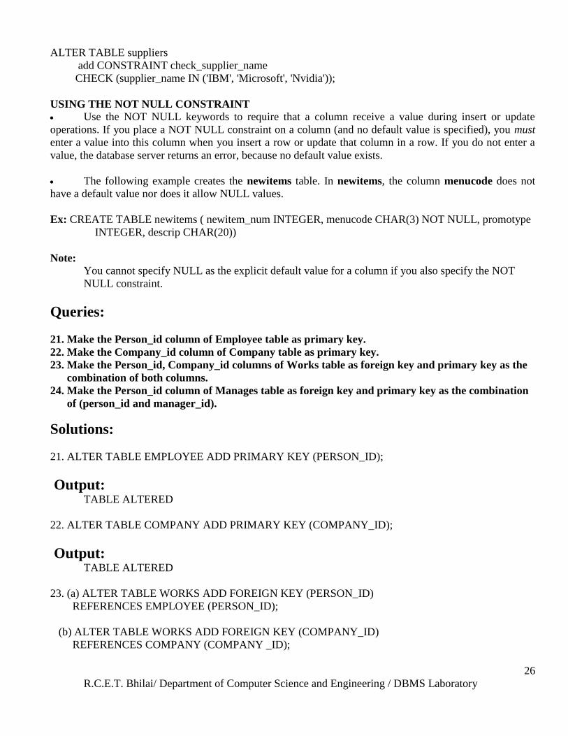
ALTER TABLE suppliers
add CONSTRAINT check_supplier_name
CHECK (supplier_name IN ('IBM', 'Microsoft', 'Nvidia'));
USING THE NOT NULL CONSTRAINT Use the NOT NULL keywords to require that a column receive a value during insert or update
operations. If you place a NOT NULL constraint on a column (and no default value is specified), you must
enter a value into this column when you insert a row or update that column in a row. If you do not enter a
value, the database server returns an error, because no default value exists.
The following example creates the newitems table. In newitems, the column menucode does not
have a default value nor does it allow NULL values.
Ex: CREATE TABLE newitems ( newitem_num INTEGER, menucode CHAR(3) NOT NULL, promotype
INTEGER, descrip CHAR(20))
Note:
You cannot specify NULL as the explicit default value for a column if you also specify the NOT
NULL constraint.
Queries:
21. Make the Person_id column of Employee table as primary key.
22. Make the Company_id column of Company table as primary key.
23. Make the Person_id, Company_id columns of Works table as foreign key and primary key as the
combination of both columns.
24. Make the Person_id column of Manages table as foreign key and primary key as the combination
of (person_id and manager_id).
Solutions:
21. ALTER TABLE EMPLOYEE ADD PRIMARY KEY (PERSON_ID);
Output: TABLE ALTERED
22. ALTER TABLE COMPANY ADD PRIMARY KEY (COMPANY_ID);
Output: TABLE ALTERED
23. (a) ALTER TABLE WORKS ADD FOREIGN KEY (PERSON_ID)
REFERENCES EMPLOYEE (PERSON_ID);
(b) ALTER TABLE WORKS ADD FOREIGN KEY (COMPANY_ID)
REFERENCES COMPANY (COMPANY _ID);
R.C.E.T. Bhilai/ Department of Computer Science and Engineering / DBMS Laboratory
27
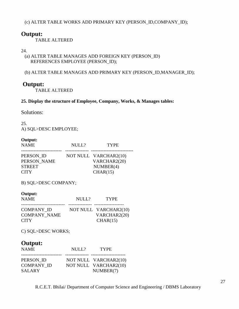
(c) ALTER TABLE WORKS ADD PRIMARY KEY (PERSON_ID,COMPANY_ID);
Output: TABLE ALTERED
24.
(a) ALTER TABLE MANAGES ADD FOREIGN KEY (PERSON_ID)
REFERENCES EMPLOYEE (PERSON_ID);
(b) ALTER TABLE MANAGES ADD PRIMARY KEY (PERSON_ID,MANAGER_ID);
Output: TABLE ALTERED
25. Display the structure of Employee, Company, Works, & Manages tables:
Solutions:
25.
A) SQL>DESC EMPLOYEE;
Output:
NAME NULL? TYPE
-------------------------- --------------- ---------------------------
PERSON_ID NOT NULL VARCHAR2(10)
PERSON_NAME VARCHAR2(20)
STREET NUMBER(4)
CITY CHAR(15)
B) SQL>DESC COMPANY;
Output:
NAME NULL? TYPE
---------------------------- --------------- -------------------
COMPANY_ID NOT NULL VARCHAR2(10)
COMPANY_NAME VARCHAR2(20)
CITY CHAR(15)
C) SQL>DESC WORKS;
Output: NAME NULL? TYPE
-------------------------- --------------- ----------------------
PERSON_ID NOT NULL VARCHAR2(10)
COMPANY_ID NOT NULL VARCHAR2(10)
SALARY NUMBER(7)
R.C.E.T. Bhilai/ Department of Computer Science and Engineering / DBMS Laboratory
28
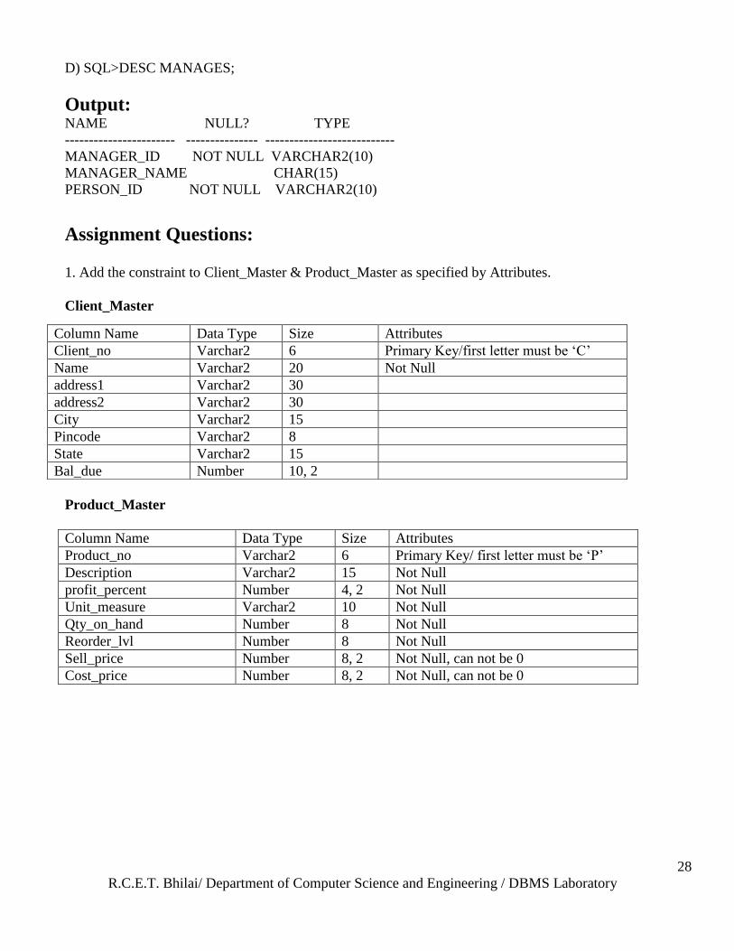
D) SQL>DESC MANAGES;
Output: NAME NULL? TYPE
----------------------- --------------- ---------------------------
MANAGER_ID NOT NULL VARCHAR2(10)
MANAGER_NAME CHAR(15)
PERSON_ID NOT NULL VARCHAR2(10)
Assignment Questions: 1. Add the constraint to Client_Master & Product_Master as specified by Attributes.
Client_Master
Product_Master
Column Name Data Type Size Attributes
Product_no Varchar2 6 Primary Key/ first letter must be ‗P‘
Description Varchar2 15 Not Null
profit_percent Number 4, 2 Not Null
Unit_measure Varchar2 10 Not Null
Qty_on_hand Number 8 Not Null
Reorder_lvl Number 8 Not Null
Sell_price Number 8, 2 Not Null, can not be 0
Cost_price Number 8, 2 Not Null, can not be 0
Column Name Data Type Size Attributes
Client_no Varchar2 6 Primary Key/first letter must be ‗C‘
Name Varchar2 20 Not Null
address1 Varchar2 30
address2 Varchar2 30
City Varchar2 15
Pincode Varchar2 8
State Varchar2 15
Bal_due Number 10, 2
R.C.E.T. Bhilai/ Department of Computer Science and Engineering / DBMS Laboratory
29
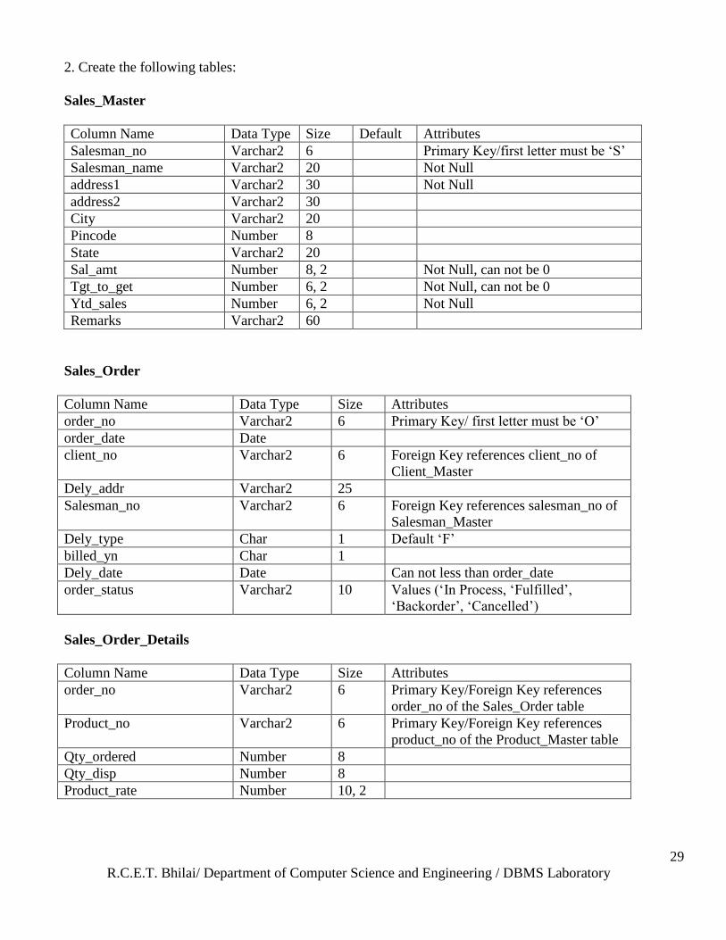
2. Create the following tables:
Sales_Master
Column Name Data Type Size Default Attributes
Salesman_no Varchar2 6 Primary Key/first letter must be ‗S‘
Salesman_name Varchar2 20 Not Null
address1 Varchar2 30 Not Null
address2 Varchar2 30
City Varchar2 20
Pincode Number 8
State Varchar2 20
Sal_amt Number 8, 2 Not Null, can not be 0
Tgt_to_get Number 6, 2 Not Null, can not be 0
Ytd_sales Number 6, 2 Not Null
Remarks Varchar2 60
Sales_Order
Column Name Data Type Size Attributes
order_no Varchar2 6 Primary Key/ first letter must be ‗O‘
order_date Date
client_no Varchar2 6 Foreign Key references client_no of
Client_Master
Dely_addr Varchar2 25
Salesman_no Varchar2 6 Foreign Key references salesman_no of
Salesman_Master
Dely_type Char 1 Default ‗F‘
billed_yn Char 1
Dely_date Date Can not less than order_date
order_status Varchar2 10 Values (‗In Process, ‗Fulfilled‘,
‗Backorder‘, ‗Cancelled‘)
Sales_Order_Details
Column Name Data Type Size Attributes
order_no Varchar2 6 Primary Key/Foreign Key references
order_no of the Sales_Order table
Product_no Varchar2 6 Primary Key/Foreign Key references
product_no of the Product_Master table
Qty_ordered Number 8
Qty_disp Number 8
Product_rate Number 10, 2
R.C.E.T. Bhilai/ Department of Computer Science and Engineering / DBMS Laboratory
30
Viva-Voce Questions:
1. What do you mean by constraints? What is the need of it.
2. What is the difference between Unique and Primary key?
3. Can the value of Foreign key be Null?
4. Is it possible to add primary key in an existing table? If Yes then how?
R.C.E.T. Bhilai/ Department of Computer Science and Engineering / DBMS Laboratory
31
Experiment No 7
Aim: Introduction to Operators used in SQL, Oracle numeric functions.
Description:
OPERATORS USED IN SQL
Arithmetic Operators:
+ Addition
- Subtraction
/ Division
* Multiplication
** Exponential
Logical Operators:
AND: SELECT * FROM STUDENT WHERE PERCENT>=65 AND PERCENT<=75;
OR: SELECT * FROM STUDENT WHERE PERCENT>=65 OR PERECNT<=75;
NOT: SELECT * FROM STUDENT WHERE NOT PERCENT<=40
RANGE SEARCHING
BETWEEN operator is used for searching data in a table within a range of values.
Ex: SELECT * FROM STUDENT WHERE PERCENT BETWEEN 85 AND 93;
PATTERN MATCHING
The LIKE predicate allows comparison of one string value with another string value. This is achieved by
using wildcard characters.
There are 2 types of wildcard characters available in SQL:
1. % -> allows to match any string of any length.
2. _ -> allows to match on a single character.
Ex1: SELECT * FROM STUDENT WHERE NAME LIKE ‗A_C%‘;
Ex2: SELECT * FROM STUDENT WHERE NAME NOT LIKE ‗D%‘;
IN and NOT IN PREDICATE
The IN predicates compares a single value to a list of values.
R.C.E.T. Bhilai/ Department of Computer Science and Engineering / DBMS Laboratory
32
Ex1: SELECT * FROM STUDENT WHERE PERCENT IN (65, 75, 85);
The NOT IN predicate the opposite of the IN predicate. This will select all the rows where values do not
match the values in the list.
Ex2: SELECT * FROM STUDENT WHERE ROLLNO NOT IN (627);
EXISTS and NOT EXISTS OPERATOR
The EXISTS condition is considered "to be met" if the sub query returns at least one row.
The syntax for the EXISTS condition is:
SELECT columns FROM tables WHERE EXISTS ( subquery );
The EXISTS condition can be used in any valid SQL statement - select, insert, update, or delete.
Ex: SELECT * FROM suppliers WHERE EXISTS (select * from orders where suppliers.supplier_id = orders.supplier_id);
This select statement will return all records from the suppliers table where there is at least one record in the
orders table with the same supplier_id.
NOT EXISTS
The EXISTS condition can also be combined with the NOT operator.
Example:
SELECT * FROM suppliers WHERE not exists (select * from orders Where suppliers.supplier_id = orders.supplier_id);
This will return all records from the suppliers table where there are no records in the orders table for the
given supplier_id.
Aggregate & numeric functions
Aggregate Functions:
1. SUM – Returns the sum of values ‗n‘.
Syntax: SUM (n)
Ex: SELECT SUM (PERCENT) FROM STUDENT;
2. AVG – Returns an average of ‗n‘, ignoring null values in a column.
Syntax: AVG (n)
Ex: SELECT AVG (PERCENT) FROM STUDENT;
3. COUNT – Returns the number of rows where expr is null.
Syntax: COUNT (expr)
R.C.E.T. Bhilai/ Department of Computer Science and Engineering / DBMS Laboratory
33
Ex: SELECT COUNT (ROLL_NO) FROM STUDENT;
4. MIN – Returns a minimum value of expr.
Syntax: MIN (expr)
Ex: SELECT MIN (PERCENT) FROM STUDENT;
5. MAX – Returns a maximum value of expr.
Syntax: MAX (expr)
Ex: SELECT MAX (PERCENT) FROM STUDENT;
Numeric functions:
Numeric functions accept numeric input and return numeric values.
1. ABS(n)
ABS returns the absolute value of n.
Example: The following example returns the absolute value of -15:
SELECT ABS(-15) "Absolute" FROM DUAL;
Absolute
----------
15
2. POWER(m,n)
POWER returns m raised to the nth power. The base m and the exponent n can be any numbers, but if m is
negative, then n must be an integer.
Example: The following example returns 3 squared:
SELECT POWER(3,2) "Raised" FROM DUAL;
Raised
----------
9
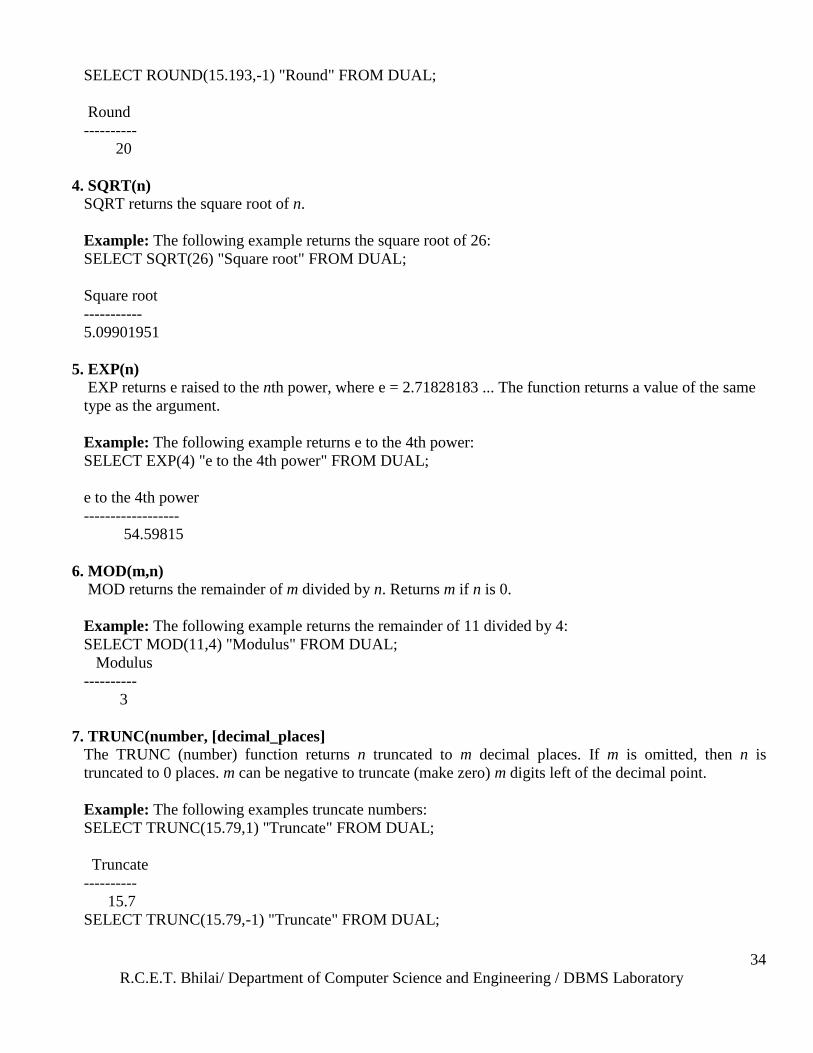
3. ROUND(n,[m])
ROUND returns n rounded to integer places to the right of the decimal point. If you omit integer, then n is
rounded to 0 places. The argument integer can be negative to round off digits left of the decimal point.
Example:
The following example rounds a number to one decimal point:
SELECT ROUND(15.193,1) "Round" FROM DUAL;
Round
----------
15.2
The following example rounds a number one digit to the left of the decimal point:
R.C.E.T. Bhilai/ Department of Computer Science and Engineering / DBMS Laboratory
34
SELECT ROUND(15.193,-1) "Round" FROM DUAL;
Round
----------
20
4. SQRT(n)
SQRT returns the square root of n.
Example: The following example returns the square root of 26:
SELECT SQRT(26) "Square root" FROM DUAL;
Square root
-----------
5.09901951
5. EXP(n)
EXP returns e raised to the nth power, where e = 2.71828183 ... The function returns a value of the same
type as the argument.
Example: The following example returns e to the 4th power:
SELECT EXP(4) "e to the 4th power" FROM DUAL;
e to the 4th power
------------------
54.59815
6. MOD(m,n) MOD returns the remainder of m divided by n. Returns m if n is 0.
Example: The following example returns the remainder of 11 divided by 4:
SELECT MOD(11,4) "Modulus" FROM DUAL;
Modulus
----------
3
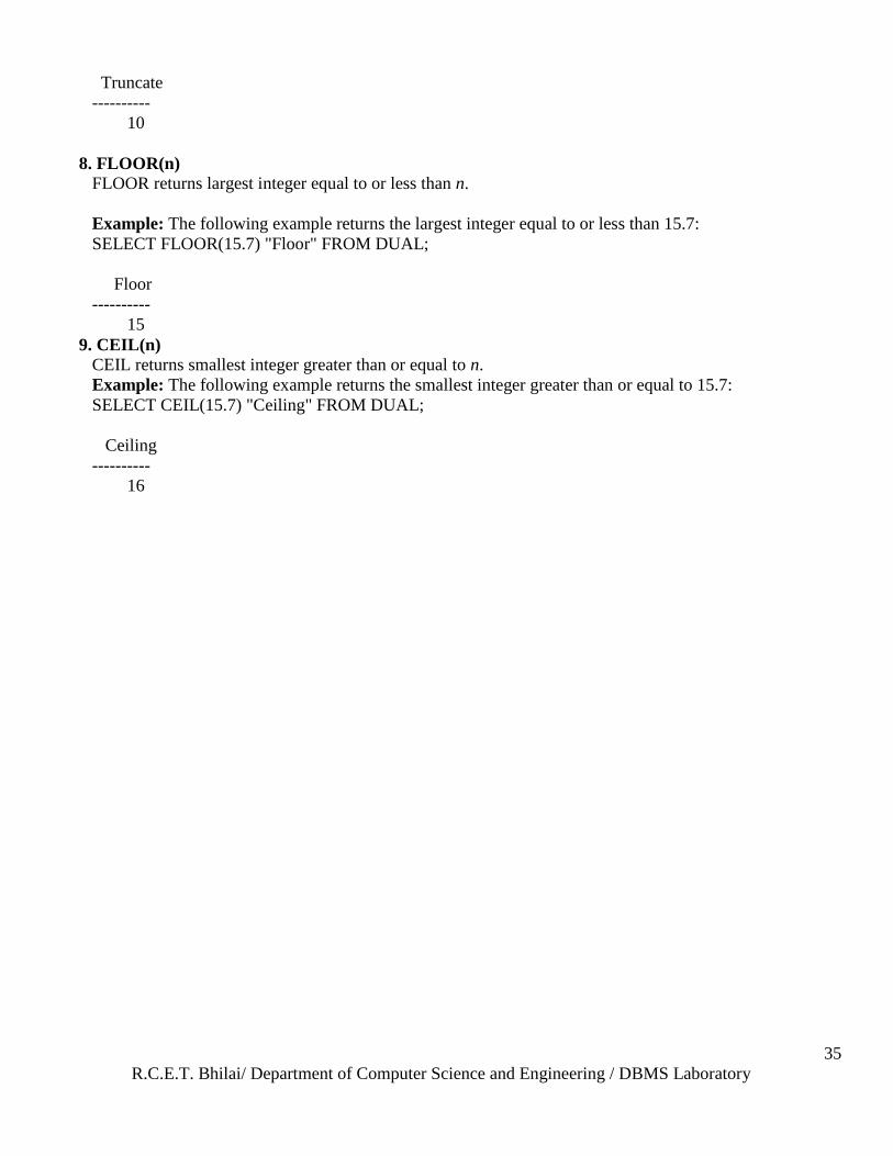
7. TRUNC(number, [decimal_places]
The TRUNC (number) function returns n truncated to m decimal places. If m is omitted, then n is
truncated to 0 places. m can be negative to truncate (make zero) m digits left of the decimal point.
Example: The following examples truncate numbers:
SELECT TRUNC(15.79,1) "Truncate" FROM DUAL;
Truncate
----------
15.7
SELECT TRUNC(15.79,-1) "Truncate" FROM DUAL;
R.C.E.T. Bhilai/ Department of Computer Science and Engineering / DBMS Laboratory
35
Truncate
----------
10
8. FLOOR(n)
FLOOR returns largest integer equal to or less than n.
Example: The following example returns the largest integer equal to or less than 15.7:
SELECT FLOOR(15.7) "Floor" FROM DUAL;
Floor
----------
15
9. CEIL(n)
CEIL returns smallest integer greater than or equal to n.
Example: The following example returns the smallest integer greater than or equal to 15.7:
SELECT CEIL(15.7) "Ceiling" FROM DUAL;
Ceiling
----------
16
R.C.E.T. Bhilai/ Department of Computer Science and Engineering / DBMS Laboratory
36
Assignment Questions:
1. Find the names of all clients having ‗a‘ as the second letter in their names.
2. Find out the clients who stay in a city whoes second letter is ‗a‘.
3. Find the list of all clients who stay in Bombay or Delhi.
4. Find the list of clients whose bal_due is greater than value 10000.
5. Find the products whose selling price is greater than 2000 and less than or equal to 5000.
6. List the names, city and state of clients who are not in the state of Maharashtra.
7. Find all the products whose qty_on_hand is less than reorder_lvl.
8. Count the number of products having price greater than or equal to 1500.
9. Calculate the average price of all the products.
10. Determine the maximum and minimum product prices. Rename the Output as max_price and
min_price respectively.
Viva-Voce Questions:
1. What do you mean by aggregate functions?
2. Functions that act on a set of values are called as _________.
3. Variables or constants accepting by functions are called _________.
4. The ________ predicate allows for a comparison of one string value with another string value, which
is not identical.
5. For character datatypes the ________ sign matches any string.
R.C.E.T. Bhilai/ Department of Computer Science and Engineering / DBMS Laboratory
37
Experiment No 8
Aim: Introduction to Oracle string & date functions.
Description:
Oracle string functions:
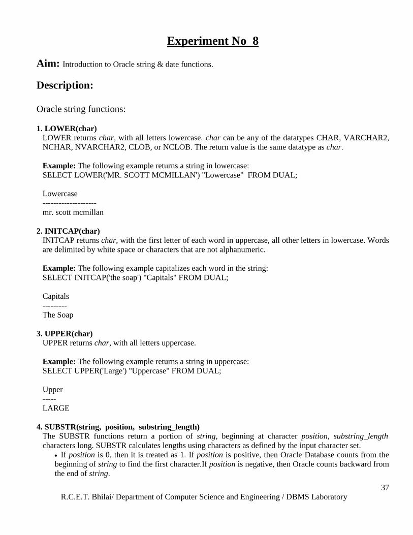
1. LOWER(char)
LOWER returns char, with all letters lowercase. char can be any of the datatypes CHAR, VARCHAR2,
NCHAR, NVARCHAR2, CLOB, or NCLOB. The return value is the same datatype as char.
Example: The following example returns a string in lowercase:
SELECT LOWER('MR. SCOTT MCMILLAN') "Lowercase" FROM DUAL;
Lowercase
--------------------
mr. scott mcmillan
2. INITCAP(char)
INITCAP returns char, with the first letter of each word in uppercase, all other letters in lowercase. Words
are delimited by white space or characters that are not alphanumeric.
Example: The following example capitalizes each word in the string:
SELECT INITCAP('the soap') "Capitals" FROM DUAL;
Capitals
---------
The Soap
3. UPPER(char)
UPPER returns char, with all letters uppercase.
Example: The following example returns a string in uppercase:
SELECT UPPER('Large') "Uppercase" FROM DUAL;
Upper
-----
LARGE
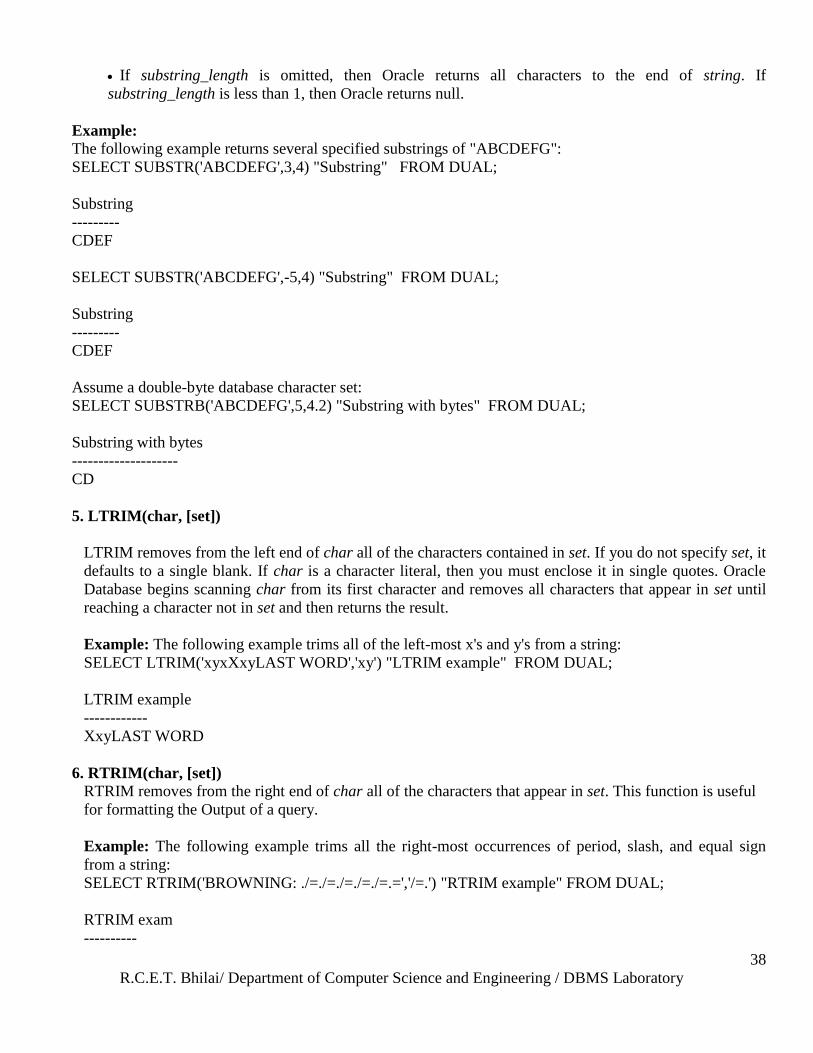
4. SUBSTR(string, position, substring_length)
The SUBSTR functions return a portion of string, beginning at character position, substring_length
characters long. SUBSTR calculates lengths using characters as defined by the input character set.
If position is 0, then it is treated as 1. If position is positive, then Oracle Database counts from the
beginning of string to find the first character.If position is negative, then Oracle counts backward from
the end of string.
R.C.E.T. Bhilai/ Department of Computer Science and Engineering / DBMS Laboratory
38
If substring_length is omitted, then Oracle returns all characters to the end of string. If
substring_length is less than 1, then Oracle returns null.
Example:
The following example returns several specified substrings of "ABCDEFG":
SELECT SUBSTR('ABCDEFG',3,4) "Substring" FROM DUAL;
Substring
---------
CDEF
SELECT SUBSTR('ABCDEFG',-5,4) "Substring" FROM DUAL;
Substring
---------
CDEF
Assume a double-byte database character set:
SELECT SUBSTRB('ABCDEFG',5,4.2) "Substring with bytes" FROM DUAL;
Substring with bytes
--------------------
CD
5. LTRIM(char, [set])
LTRIM removes from the left end of char all of the characters contained in set. If you do not specify set, it
defaults to a single blank. If char is a character literal, then you must enclose it in single quotes. Oracle
Database begins scanning char from its first character and removes all characters that appear in set until
reaching a character not in set and then returns the result.
Example: The following example trims all of the left-most x's and y's from a string:
SELECT LTRIM('xyxXxyLAST WORD','xy') "LTRIM example" FROM DUAL;
LTRIM example
------------
XxyLAST WORD
6. RTRIM(char, [set])
RTRIM removes from the right end of char all of the characters that appear in set. This function is useful
for formatting the Output of a query.
Example: The following example trims all the right-most occurrences of period, slash, and equal sign
from a string:
SELECT RTRIM('BROWNING: ./=./=./=./=./=.=','/=.') "RTRIM example" FROM DUAL;
RTRIM exam
----------
R.C.E.T. Bhilai/ Department of Computer Science and Engineering / DBMS Laboratory
39
BROWNING:
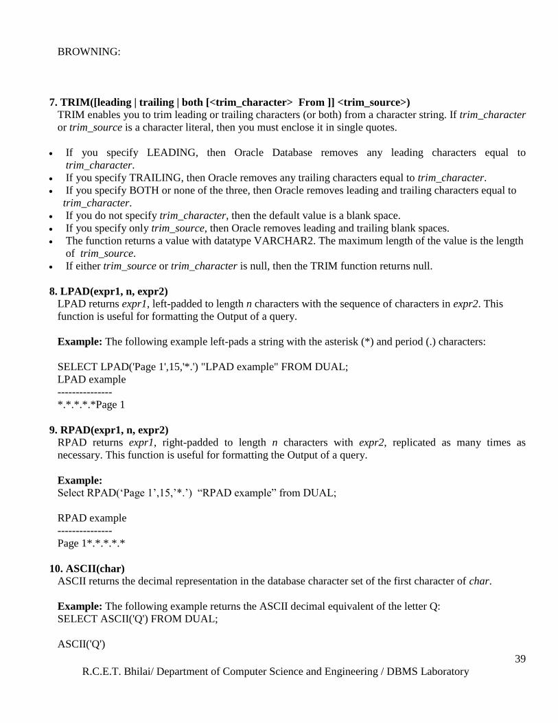
7. TRIM([leading | trailing | both [<trim_character> From ]] <trim_source>)
TRIM enables you to trim leading or trailing characters (or both) from a character string. If trim_character
or trim_source is a character literal, then you must enclose it in single quotes.
If you specify LEADING, then Oracle Database removes any leading characters equal to
trim_character.
If you specify TRAILING, then Oracle removes any trailing characters equal to trim_character.
If you specify BOTH or none of the three, then Oracle removes leading and trailing characters equal to
trim_character.
If you do not specify trim_character, then the default value is a blank space.
If you specify only trim_source, then Oracle removes leading and trailing blank spaces.
The function returns a value with datatype VARCHAR2. The maximum length of the value is the length
of trim_source.
If either trim_source or trim_character is null, then the TRIM function returns null.
8. LPAD(expr1, n, expr2)
LPAD returns expr1, left-padded to length n characters with the sequence of characters in expr2. This
function is useful for formatting the Output of a query.
Example: The following example left-pads a string with the asterisk (*) and period (.) characters:
SELECT LPAD('Page 1',15,'*.') "LPAD example" FROM DUAL;
LPAD example
---------------
*.*.*.*.*Page 1
9. RPAD(expr1, n, expr2)
RPAD returns expr1, right-padded to length n characters with expr2, replicated as many times as
necessary. This function is useful for formatting the Output of a query.
Example:
Select RPAD(‗Page 1‘,15,‘*.‘) ―RPAD example‖ from DUAL;
RPAD example
---------------
Page 1*.*.*.*.*
10. ASCII(char)
ASCII returns the decimal representation in the database character set of the first character of char.
Example: The following example returns the ASCII decimal equivalent of the letter Q:
SELECT ASCII('Q') FROM DUAL;
ASCII('Q')
R.C.E.T. Bhilai/ Department of Computer Science and Engineering / DBMS Laboratory
40
----------
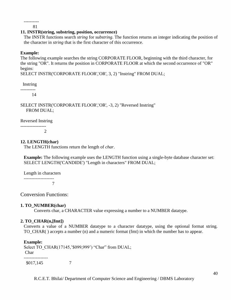
81
11. INSTR(string, substring, position, occurrence)
The INSTR functions search string for substring. The function returns an integer indicating the position of
the character in string that is the first character of this occurrence.
Example:
The following example searches the string CORPORATE FLOOR, beginning with the third character, for
the string "OR". It returns the position in CORPORATE FLOOR at which the second occurrence of "OR"
begins:
SELECT INSTR('CORPORATE FLOOR','OR', 3, 2) "Instring" FROM DUAL;
Instring
----------
14
SELECT INSTR('CORPORATE FLOOR','OR', -3, 2) "Reversed Instring"
FROM DUAL;
Reversed Instring
-----------------
2
12. LENGTH(char)
The LENGTH functions return the length of char.
Example: The following example uses the LENGTH function using a single-byte database character set:
SELECT LENGTH('CANDIDE') "Length in characters" FROM DUAL;
Length in characters
--------------------
7
Conversion Functions:
1. TO_NUMBER(char)
Converts char, a CHARACTER value expressing a number to a NUMBER datatype.
2. TO_CHAR(n,[fmt])
Converts a value of a NUMBER datatype to a character datatype, using the optional format string.
TO_CHAR( ) accepts a number (n) and a numeric format (fmt) in which the number has to appear.
Example:
Select TO_CHAR(17145,‘$099,999‘) ―Char‖ from DUAL;
Char
----------------
$017,145 7
R.C.E.T. Bhilai/ Department of Computer Science and Engineering / DBMS Laboratory
41
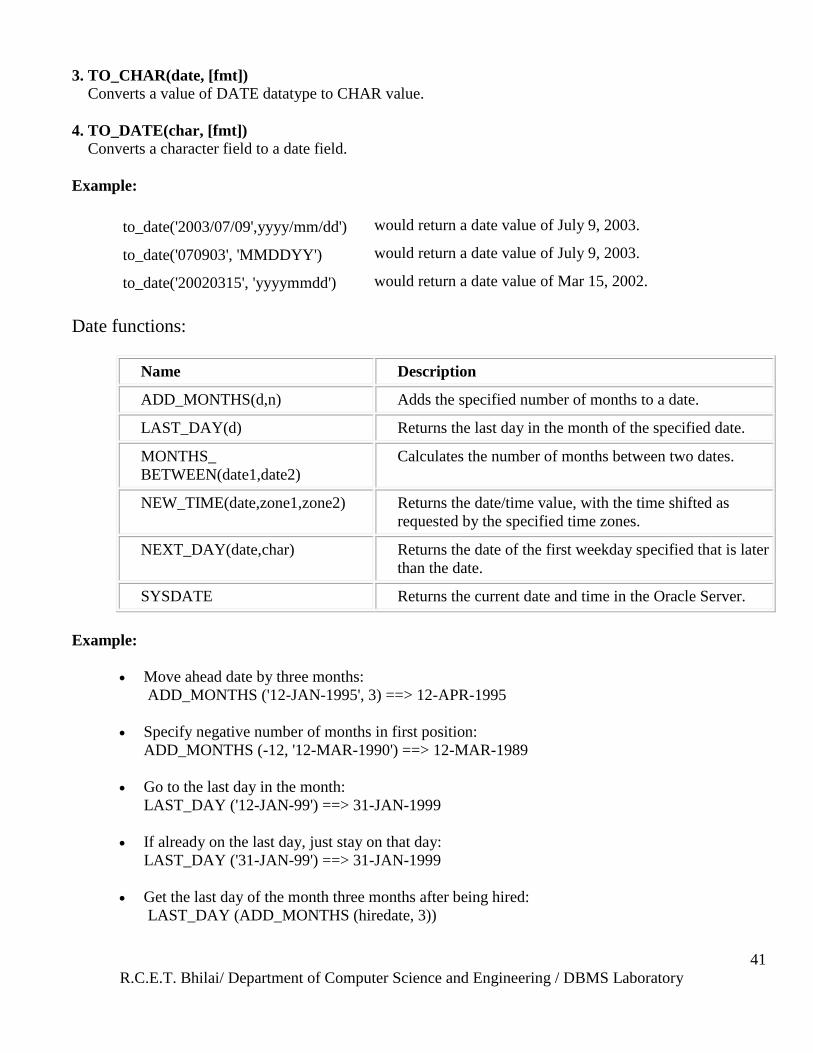
3. TO_CHAR(date, [fmt])
Converts a value of DATE datatype to CHAR value.
4. TO_DATE(char, [fmt])
Converts a character field to a date field.
Example:
to_date('2003/07/09',yyyy/mm/dd') would return a date value of July 9, 2003.
to_date('070903', 'MMDDYY') would return a date value of July 9, 2003.
to_date('20020315', 'yyyymmdd') would return a date value of Mar 15, 2002.
Date functions:
Name Description
ADD_MONTHS(d,n) Adds the specified number of months to a date.
LAST_DAY(d) Returns the last day in the month of the specified date.
MONTHS_
BETWEEN(date1,date2)
Calculates the number of months between two dates.
NEW_TIME(date,zone1,zone2) Returns the date/time value, with the time shifted as
requested by the specified time zones.
NEXT_DAY(date,char) Returns the date of the first weekday specified that is later
than the date.
SYSDATE Returns the current date and time in the Oracle Server.
Example:
Move ahead date by three months:
ADD_MONTHS ('12-JAN-1995', 3) ==> 12-APR-1995
Specify negative number of months in first position:
ADD_MONTHS (-12, '12-MAR-1990') ==> 12-MAR-1989
Go to the last day in the month:
LAST_DAY ('12-JAN-99') ==> 31-JAN-1999
If already on the last day, just stay on that day:
LAST_DAY ('31-JAN-99') ==> 31-JAN-1999
Get the last day of the month three months after being hired:
LAST_DAY (ADD_MONTHS (hiredate, 3))

R.C.E.T. Bhilai/ Department of Computer Science and Engineering / DBMS Laboratory
42
Tell me the number of days until the end of the month:
LAST_DAY (SYSDATE) – SYSDATE
Calculate two ends of month, the first earlier than the second:
MONTHS_BETWEEN ('31-JAN-1994', '28-FEB-1994') ==> -1
Calculate two ends of month, the first later than the second:
MONTHS_BETWEEN ('31-MAR-1995', '28-FEB-1994') ==> 13
Calculate when both dates fall in the same month:
MONTHS_BETWEEN ('28-FEB-1994', '15-FEB-1994') ==> 0
Perform months_between calculations with a fractional component:
MONTHS_BETWEEN ('31-JAN-1994', '1-MAR-1994') ==> -1.0322581
MONTHS_BETWEEN ('31-JAN-1994', '2-MAR-1994') ==> -1.0645161
MONTHS_BETWEEN ('31-JAN-1994', '10-MAR-1994') ==> -1.3225806
TO_CHAR (NEW_TIME (TO_DATE ('09151994 12:30 AM', 'MMDDYYYY HH:MI AM'),
'CST', 'hdt'), 'Month DD, YYYY HH:MI AM')
==> 'September 14, 1994 09:30 PM'
You can use both full and abbreviated day names:
NEXT_DAY ('01-JAN-1997', 'MONDAY') ==> 06-JAN-1997
NEXT_DAY ('01-JAN-1997', 'MON') ==> 06-JAN-1997
The case of the day name doesn't matter a whit:
NEXT_DAY ('01-JAN-1997', 'monday') ==> 06-JAN-1997
If the date language were Spanish:
NEXT_DAY ('01-JAN-1997', 'LUNES') ==> 06-JAN-1997
NEXT_DAY of Wednesday moves the date up a full week:
NEXT_DAY ('01-JAN-1997', 'WEDNESDAY') ==> 08-JAN-1997
R.C.E.T. Bhilai/ Department of Computer Science and Engineering / DBMS Laboratory
43
Assignment Questions: 1. List the order number and day on which clients placed their order.
2. List the month(in alphabets) and date when the orders must be delivered.
3. List the Order date in the format ‗DD-Month-YY‘ e.g. 12-February-08.
4. List the date, 15 days after today‘s date.
5. Add Mr. to all the names in Client_Master.
Viva-Voce Questions: 1. The __________ function converts a value of a Date data type to CHAR value.
2. The ___________ function returns number of months between two dates.
3. The __________ function converts char a Character value expressing a number to a Number data type.
4. The __________ function returns a string with the first letter of each word in upper case.
5. The __________ function removes characters from the left of char with initial characters removed upto
the first character not in set.

R.C.E.T. Bhilai/ Department of Computer Science and Engineering / DBMS Laboratory
44
Experiment No 9
Aim: Introduction to Grouping data and Sub queries.
Description:
GROUP BY CLAUSE
This clause is used to filter data. This clause creates a data set , containing several sets of records grouped
together based on a condition.
Syntax:
SELECT <ColumnName1>, <ColumnName2>, <ColumnName1>,Aggregate_Function
(<Expression>) GROUP BY <ColumnName1>, <ColumnName2>, <ColumnNameN>;
Ex: SELECT PERCENT, COUNT (ROLL_NO) ―No.of Students‖ FROM STUDENT
GROUP BY PERCENT;
Example using the SUM function
SELECT department, SUM(sales) as "Total sales" FROM order_details GROUP BY department;
Example using the COUNT function
SELECT department, COUNT(*) as "Number of employees" FROM employees WHERE salary > 25000 GROUP BY department;
Example using the MIN function
SELECT department, MIN(salary) as "Lowest salary" FROM employees GROUP BY department;
Example using the MAX function
SELECT department, MAX(salary) as "Highest salary" FROM employees GROUP BY department;
HAVING CLAUSE
This can be used in conjunction with the GROUP BY clause. Having imposes (puts) a condition on the
GROUP BY clause, which further filters the groups created by the Group By clause.
R.C.E.T. Bhilai/ Department of Computer Science and Engineering / DBMS Laboratory
45
Syntax:
SELECT <ColumnName1>, <ColumnName2>, <ColumnName1>,Aggregate_Function
(<Expression>) GROUP BY <ColumnName1>, <ColumnName2>, <ColumnNameN> HAVING
<Condition>;
Ex: SELECT PERCENT, COUNT (ROLL_NO) ―No.of Students‖ FROM STUDENTGROUP BY
PERCENT
HAVING ROLL_NO > 15;
SUB-QUERY
A Sub-query is the form of an SQL statement that appears inside another SQL statement. It is also termed as
nested query.
It can be used for the following:
To insert records in a target table.
To create tables & insert records in the table created.
To update records in a target table.
To create views.
To provide values for conditions in WHERE, HAVING, IN & so on used with SELECT, UPDATE
&
DELETE statements.=
Ex1: SELECT * FROM employees WHERE id = (SELECT EmployeeID FROM invoices WHERE EmployeeID =1 );
Ex2: SELECT MODEL FROM PRODUCT WHERE ManufactureID IN (SELECT ManufactureID FROM Manufacturer WHERE Manufacturer = ‘DELL’)
Ex3: SELECT SUM(Sales) FROM Store_Information WHERE Store_name IN (SELECT store_name FROM Geography WHERE region_name = 'West')
R.C.E.T. Bhilai/ Department of Computer Science and Engineering / DBMS Laboratory
46
Assignment Questions: Exercise on using Having and Group By Clauses:
1. Print the description and total qty sold for each product.
2. Find the value of each product sold.
3. Calculate the average qty sold for each client that has a maximum order value of
15000.00.
4. Find out the sum total of all the billed orders for the month of January.
Exercise on sub-queries:
a) Find the customer name, address1, address2, city and pincode for the client who hase placed order_no
‗O19001‘.
b) Find the client names who have placed orders before the month of May‘96.
c) Find the names of clients who have placed orders worth rs. 10000 or more.
Viva-Voce Questions:
1. Are the following statements true or false?
The aggregate functions SUM, COUNT, MIN, MAX, and AVG all return multiple values.
The maximum number of subqueries that can be nested is two.
Correlated subqueries are completely self-contained.
R.C.E.T. Bhilai/ Department of Computer Science and Engineering / DBMS Laboratory
47
Experiment No 10
Aim: Introduction to Joins.
Description:
JOINS
Joins are used to work with multiple tables as though they were a single entity. Tables are joined on
columns that have the same data type and data width in the tables.
.
Types of Joins –
Equi Join
Inner Join
Outer Join
Cross Join
Self Join
Inner join
An inner join does require each record in the two joined tables to have a matching record. An inner join
essentially combines the records from two tables (A and B) based on a given join-predicate. The SQL-
engine computes the Cartesian product of all records in the tables. Thus, processing combines each record in
table A with every record in table B. Only those records in the joined table that satisfy the join predicate
remain. This type of join occurs most commonly in applications, and represents the default join-type.
SQL specifies two different syntactical ways to express joins. The first, called "explicit join notation", uses
the keyword JOIN, whereas the second uses the "implicit join notation". The implicit join notation lists the
tables for joining in the FROM clause of a SELECT statement, using commas to separate them. Thus, it always
computes a cross-join, and the WHERE clause may apply additional filter-predicates. Those filter-predicates
function comparably to join-predicates in the explicit notation.
One can further classify inner joins as equi-joins, as natural joins, or as cross-joins.
Programmers should take special care when joining tables on columns that can contain NULL values, since
NULL will never match any other value (or even NULL itself), unless the join condition explicitly uses the
IS NULL or IS NOT NULL predicates.
As an example, the following query takes all the records from the Employee table and finds the matching
record(s) in the Department table, based on the join predicate. The join predicate compares the values in the
DepartmentID column in both tables. If it finds no match (i.e., the department-id of an employee does not
match the current department-id from the Department table), then the joined record remains outside the
joined table, i.e., outside the (intermediate) result of the join.
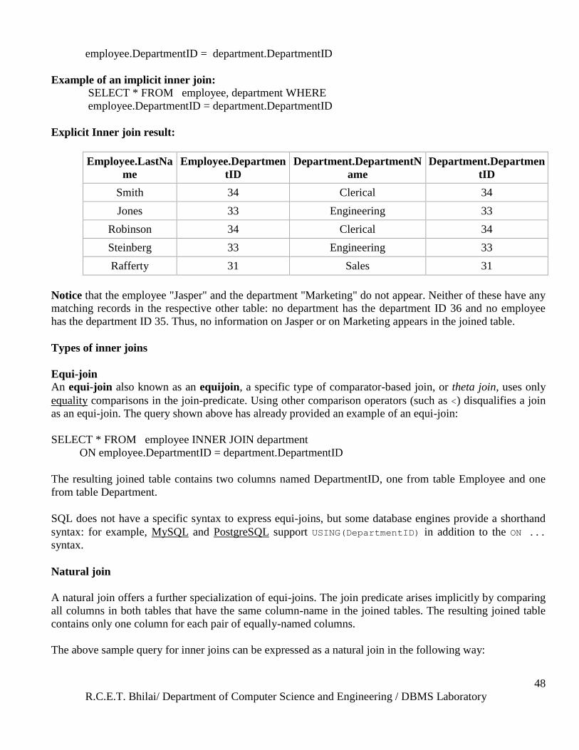
Example of an explicit inner join:
SELECT * FROM employee INNER JOIN department ON
R.C.E.T. Bhilai/ Department of Computer Science and Engineering / DBMS Laboratory
48
employee.DepartmentID = department.DepartmentID
Example of an implicit inner join:
SELECT * FROM employee, department WHERE
employee.DepartmentID = department.DepartmentID
Explicit Inner join result:
Employee.LastNa
me
Employee.Departmen
tID
Department.DepartmentN
ame
Department.Departmen
tID
Smith 34 Clerical 34
Jones 33 Engineering 33
Robinson 34 Clerical 34
Steinberg 33 Engineering 33
Rafferty 31 Sales 31
Notice that the employee "Jasper" and the department "Marketing" do not appear. Neither of these have any
matching records in the respective other table: no department has the department ID 36 and no employee
has the department ID 35. Thus, no information on Jasper or on Marketing appears in the joined table.
Types of inner joins
Equi-join
An equi-join also known as an equijoin, a specific type of comparator-based join, or theta join, uses only
equality comparisons in the join-predicate. Using other comparison operators (such as <) disqualifies a join
as an equi-join. The query shown above has already provided an example of an equi-join:
SELECT * FROM employee INNER JOIN department
ON employee.DepartmentID = department.DepartmentID
The resulting joined table contains two columns named DepartmentID, one from table Employee and one
from table Department.
SQL does not have a specific syntax to express equi-joins, but some database engines provide a shorthand
syntax: for example, MySQL and PostgreSQL support USING(DepartmentID) in addition to the ON ...
syntax.
Natural join
A natural join offers a further specialization of equi-joins. The join predicate arises implicitly by comparing
all columns in both tables that have the same column-name in the joined tables. The resulting joined table
contains only one column for each pair of equally-named columns.
The above sample query for inner joins can be expressed as a natural join in the following way:
R.C.E.T. Bhilai/ Department of Computer Science and Engineering / DBMS Laboratory
49
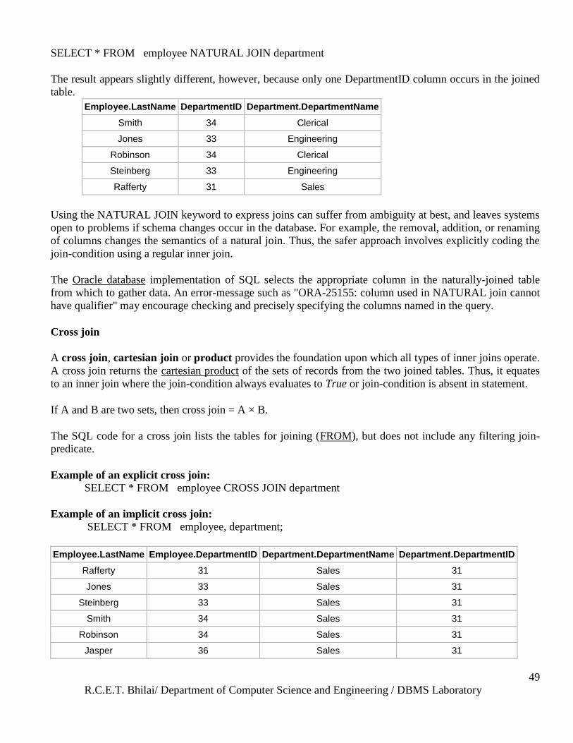
SELECT * FROM employee NATURAL JOIN department
The result appears slightly different, however, because only one DepartmentID column occurs in the joined
table.
Employee.LastName DepartmentID Department.DepartmentName
Smith 34 Clerical
Jones 33 Engineering
Robinson 34 Clerical
Steinberg 33 Engineering
Rafferty 31 Sales
Using the NATURAL JOIN keyword to express joins can suffer from ambiguity at best, and leaves systems
open to problems if schema changes occur in the database. For example, the removal, addition, or renaming
of columns changes the semantics of a natural join. Thus, the safer approach involves explicitly coding the
join-condition using a regular inner join.
The Oracle database implementation of SQL selects the appropriate column in the naturally-joined table
from which to gather data. An error-message such as "ORA-25155: column used in NATURAL join cannot
have qualifier" may encourage checking and precisely specifying the columns named in the query.
Cross join
A cross join, cartesian join or product provides the foundation upon which all types of inner joins operate.
A cross join returns the cartesian product of the sets of records from the two joined tables. Thus, it equates
to an inner join where the join-condition always evaluates to True or join-condition is absent in statement.
If A and B are two sets, then cross join = A × B.
The SQL code for a cross join lists the tables for joining (FROM), but does not include any filtering join-
predicate.
Example of an explicit cross join:
SELECT * FROM employee CROSS JOIN department
Example of an implicit cross join:
SELECT * FROM employee, department;
Employee.LastName Employee.DepartmentID Department.DepartmentName Department.DepartmentID
Rafferty 31 Sales 31
Jones 33 Sales 31
Steinberg 33 Sales 31
Smith 34 Sales 31
Robinson 34 Sales 31
Jasper 36 Sales 31
R.C.E.T. Bhilai/ Department of Computer Science and Engineering / DBMS Laboratory
50
Rafferty 31 Engineering 33
Jones 33 Engineering 33
Steinberg 33 Engineering 33
Smith 34 Engineering 33
Robinson 34 Engineering 33
Jasper 36 Engineering 33
Rafferty 31 Clerical 34
Jones 33 Clerical 34
Steinberg 33 Clerical 34
Smith 34 Clerical 34
Robinson 34 Clerical 34
Jasper 36 Clerical 34
Rafferty 31 Marketing 35
Jones 33 Marketing 35
Steinberg 33 Marketing 35
Smith 34 Marketing 35
Robinson 34 Marketing 35
Jasper 36 Marketing 35
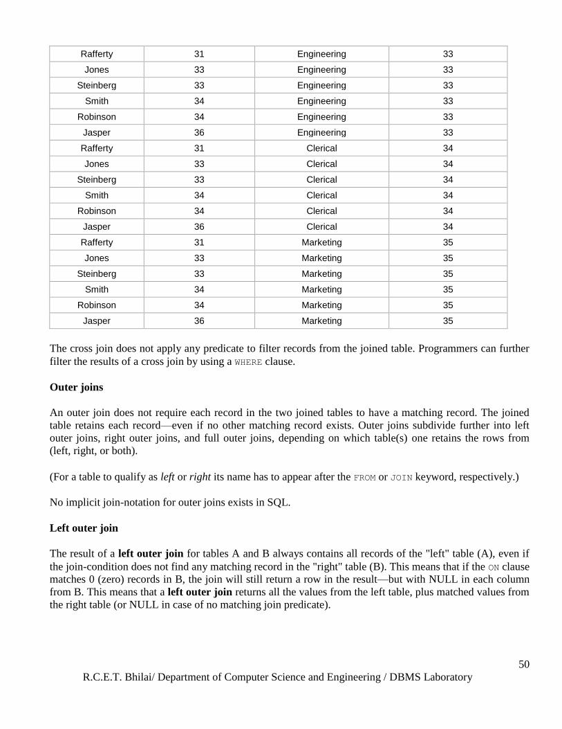
The cross join does not apply any predicate to filter records from the joined table. Programmers can further
filter the results of a cross join by using a WHERE clause.
Outer joins
An outer join does not require each record in the two joined tables to have a matching record. The joined
table retains each record—even if no other matching record exists. Outer joins subdivide further into left
outer joins, right outer joins, and full outer joins, depending on which table(s) one retains the rows from
(left, right, or both).
(For a table to qualify as left or right its name has to appear after the FROM or JOIN keyword, respectively.)
No implicit join-notation for outer joins exists in SQL.
Left outer join
The result of a left outer join for tables A and B always contains all records of the "left" table (A), even if
the join-condition does not find any matching record in the "right" table (B). This means that if the ON clause
matches 0 (zero) records in B, the join will still return a row in the result—but with NULL in each column
from B. This means that a left outer join returns all the values from the left table, plus matched values from
the right table (or NULL in case of no matching join predicate).
R.C.E.T. Bhilai/ Department of Computer Science and Engineering / DBMS Laboratory
51
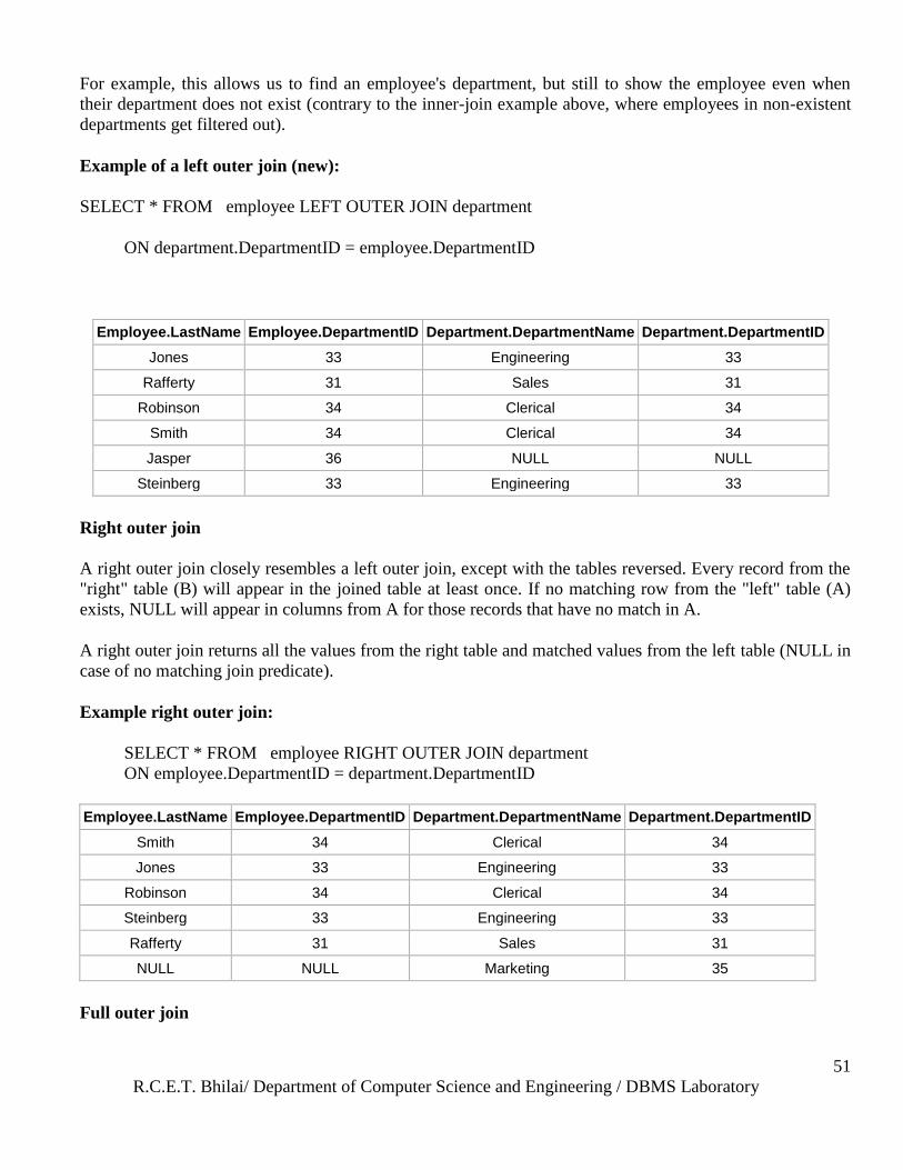
For example, this allows us to find an employee's department, but still to show the employee even when
their department does not exist (contrary to the inner-join example above, where employees in non-existent
departments get filtered out).
Example of a left outer join (new):
SELECT * FROM employee LEFT OUTER JOIN department
ON department.DepartmentID = employee.DepartmentID
Employee.LastName Employee.DepartmentID Department.DepartmentName Department.DepartmentID
Jones 33 Engineering 33
Rafferty 31 Sales 31
Robinson 34 Clerical 34
Smith 34 Clerical 34
Jasper 36 NULL NULL
Steinberg 33 Engineering 33
Right outer join
A right outer join closely resembles a left outer join, except with the tables reversed. Every record from the
"right" table (B) will appear in the joined table at least once. If no matching row from the "left" table (A)
exists, NULL will appear in columns from A for those records that have no match in A.
A right outer join returns all the values from the right table and matched values from the left table (NULL in
case of no matching join predicate).
Example right outer join:
SELECT * FROM employee RIGHT OUTER JOIN department
ON employee.DepartmentID = department.DepartmentID
Employee.LastName Employee.DepartmentID Department.DepartmentName Department.DepartmentID
Smith 34 Clerical 34
Jones 33 Engineering 33
Robinson 34 Clerical 34
Steinberg 33 Engineering 33
Rafferty 31 Sales 31
NULL NULL Marketing 35
Full outer join
R.C.E.T. Bhilai/ Department of Computer Science and Engineering / DBMS Laboratory
52
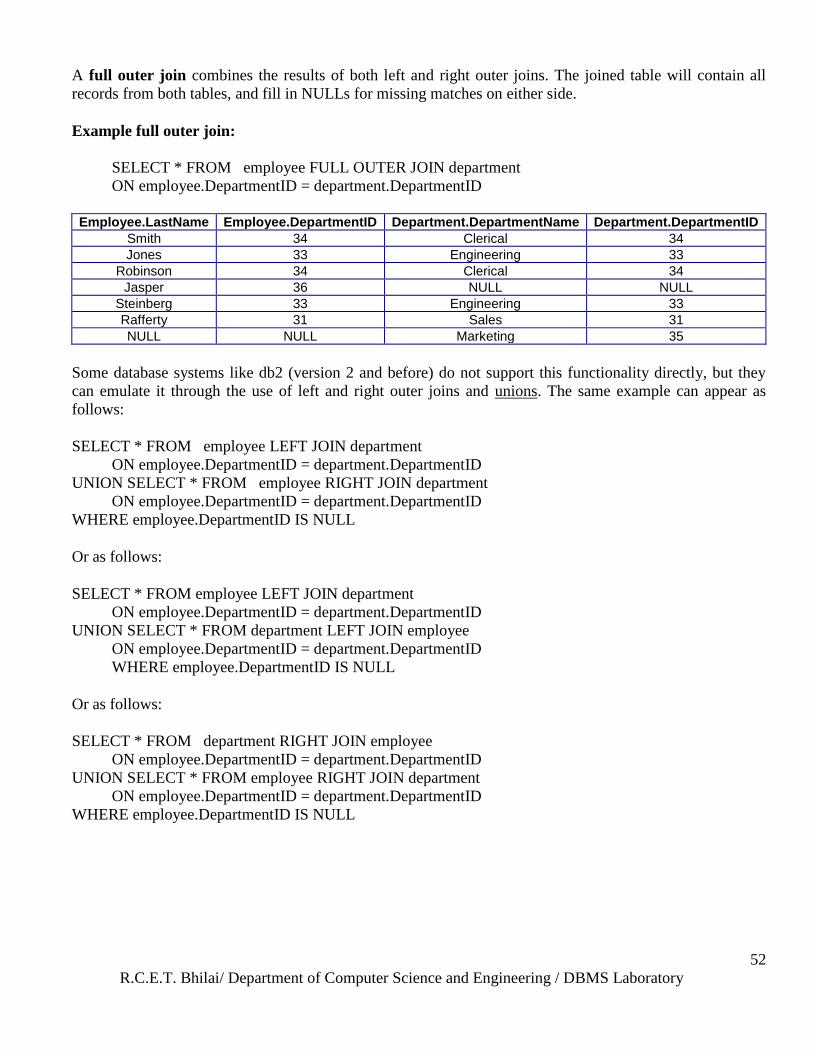
A full outer join combines the results of both left and right outer joins. The joined table will contain all
records from both tables, and fill in NULLs for missing matches on either side.
Example full outer join:
SELECT * FROM employee FULL OUTER JOIN department
ON employee.DepartmentID = department.DepartmentID
Employee.LastName Employee.DepartmentID Department.DepartmentName Department.DepartmentID
Smith 34 Clerical 34
Jones 33 Engineering 33
Robinson 34 Clerical 34
Jasper 36 NULL NULL
Steinberg 33 Engineering 33
Rafferty 31 Sales 31
NULL NULL Marketing 35
Some database systems like db2 (version 2 and before) do not support this functionality directly, but they
can emulate it through the use of left and right outer joins and unions. The same example can appear as
follows:
SELECT * FROM employee LEFT JOIN department
ON employee.DepartmentID = department.DepartmentID
UNION SELECT * FROM employee RIGHT JOIN department
ON employee.DepartmentID = department.DepartmentID
WHERE employee.DepartmentID IS NULL
Or as follows:
SELECT * FROM employee LEFT JOIN department
ON employee.DepartmentID = department.DepartmentID
UNION SELECT * FROM department LEFT JOIN employee
ON employee.DepartmentID = department.DepartmentID
WHERE employee.DepartmentID IS NULL
Or as follows:
SELECT * FROM department RIGHT JOIN employee
ON employee.DepartmentID = department.DepartmentID
UNION SELECT * FROM employee RIGHT JOIN department
ON employee.DepartmentID = department.DepartmentID
WHERE employee.DepartmentID IS NULL
R.C.E.T. Bhilai/ Department of Computer Science and Engineering / DBMS Laboratory
53
Queries:
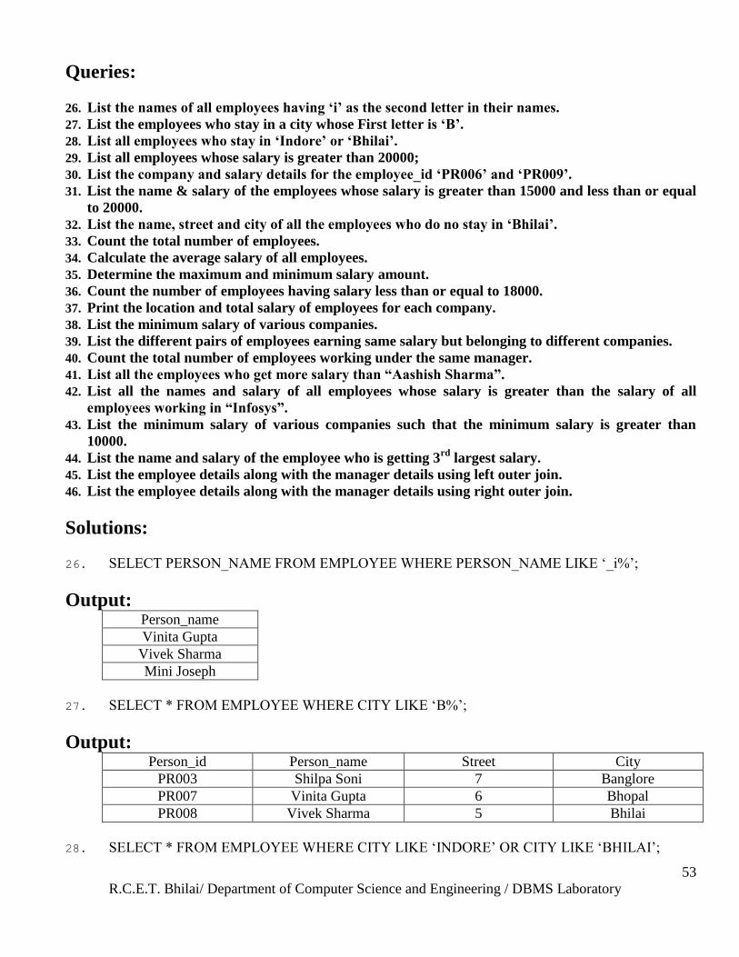
26. List the names of all employees having „i‟ as the second letter in their names.
27. List the employees who stay in a city whose First letter is „B‟.
28. List all employees who stay in „Indore‟ or „Bhilai‟.
29. List all employees whose salary is greater than 20000;
30. List the company and salary details for the employee_id „PR006‟ and „PR009‟.
31. List the name & salary of the employees whose salary is greater than 15000 and less than or equal
to 20000.
32. List the name, street and city of all the employees who do no stay in „Bhilai‟.
33. Count the total number of employees.
34. Calculate the average salary of all employees.
35. Determine the maximum and minimum salary amount.
36. Count the number of employees having salary less than or equal to 18000.
37. Print the location and total salary of employees for each company.
38. List the minimum salary of various companies.
39. List the different pairs of employees earning same salary but belonging to different companies.
40. Count the total number of employees working under the same manager.
41. List all the employees who get more salary than “Aashish Sharma”.
42. List all the names and salary of all employees whose salary is greater than the salary of all
employees working in “Infosys”.
43. List the minimum salary of various companies such that the minimum salary is greater than
10000.
44. List the name and salary of the employee who is getting 3rd
largest salary.
45. List the employee details along with the manager details using left outer join.
46. List the employee details along with the manager details using right outer join.
Solutions:
26. SELECT PERSON_NAME FROM EMPLOYEE WHERE PERSON_NAME LIKE ‗_i%‘;
Output: Person_name
Vinita Gupta
Vivek Sharma
Mini Joseph
27. SELECT * FROM EMPLOYEE WHERE CITY LIKE ‗B%‘;
Output: Person_id Person_name Street City
PR003 Shilpa Soni 7 Banglore
PR007 Vinita Gupta 6 Bhopal
PR008 Vivek Sharma 5 Bhilai
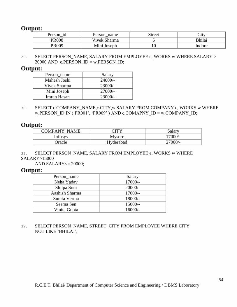
28. SELECT * FROM EMPLOYEE WHERE CITY LIKE ‗INDORE‘ OR CITY LIKE ‗BHILAI‘;
R.C.E.T. Bhilai/ Department of Computer Science and Engineering / DBMS Laboratory
54
Output: Person_id Person_name Street City
PR008 Vivek Sharma 5 Bhilai
PR009 Mini Joseph 10 Indore
29. SELECT PERSON_NAME, SALARY FROM EMPLOYEE e, WORKS w WHERE SALARY >
20000 AND e.PERSON_ID = w.PERSON_ID;
Output: Person_name Salary
Mahesh Joshi 24000/-
Vivek Sharma 23000/-
Mini Joseph 27000/-
Imran Hasan 23000/-
30. SELECT c.COMPANY_NAME,c.CITY,w.SALARY FROM COMPANY c, WORKS w WHERE
w.PERSON_ID IN (‗PR001‘, ‗PR009‘ ) AND c.COMAPNY_ID = w.COMPANY_ID;
Output: COMPANY_NAME CITY Salary
Infosys Mysore 17000/-
Oracle Hyderabad 27000/-
31. SELECT PERSON_NAME, SALARY FROM EMPLOYEE e, WORKS w WHERE
SALARY>15000
AND SALARY<= 20000;
Output: Person_name Salary
Neha Yadav 17000/-
Shilpa Soni 20000/-
Aashish Sharma 17000/-
Sunita Verma 18000/-
Seema Sen 15000/-
Vinita Gupta 16000/-
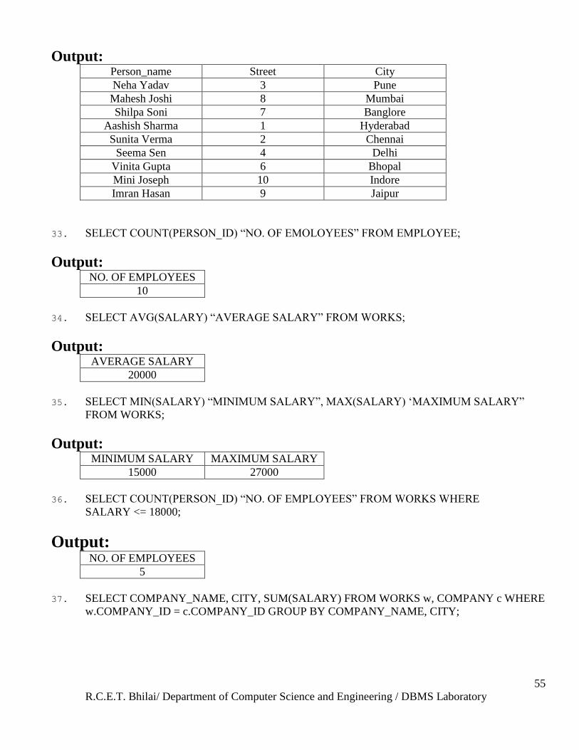
32. SELECT PERSON_NAME, STREET, CITY FROM EMPLOYEE WHERE CITY
NOT LIKE ‗BHILAI‘;
R.C.E.T. Bhilai/ Department of Computer Science and Engineering / DBMS Laboratory
55
Output: Person_name Street City
Neha Yadav 3 Pune
Mahesh Joshi 8 Mumbai
Shilpa Soni 7 Banglore
Aashish Sharma 1 Hyderabad
Sunita Verma 2 Chennai
Seema Sen 4 Delhi
Vinita Gupta 6 Bhopal
Mini Joseph 10 Indore
Imran Hasan 9 Jaipur
33. SELECT COUNT(PERSON_ID) ―NO. OF EMOLOYEES‖ FROM EMPLOYEE;
Output: NO. OF EMPLOYEES
10
34. SELECT AVG(SALARY) ―AVERAGE SALARY‖ FROM WORKS;
Output: AVERAGE SALARY
20000
35. SELECT MIN(SALARY) ―MINIMUM SALARY‖, MAX(SALARY) ‗MAXIMUM SALARY‖
FROM WORKS;
Output: MINIMUM SALARY MAXIMUM SALARY
15000 27000
36. SELECT COUNT(PERSON_ID) ―NO. OF EMPLOYEES‖ FROM WORKS WHERE
SALARY <= 18000;
Output: NO. OF EMPLOYEES
5
37. SELECT COMPANY_NAME, CITY, SUM(SALARY) FROM WORKS w, COMPANY c WHERE
w.COMPANY_ID = c.COMPANY_ID GROUP BY COMPANY_NAME, CITY;
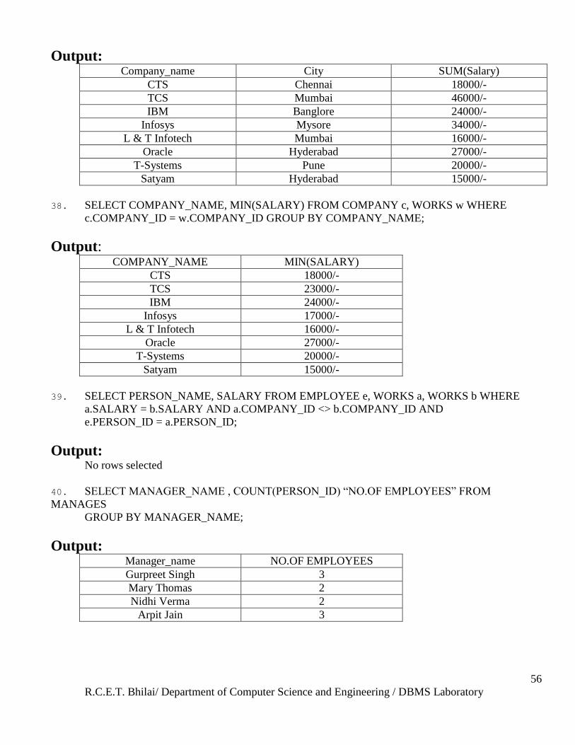
R.C.E.T. Bhilai/ Department of Computer Science and Engineering / DBMS Laboratory
56
Output: Company_name City SUM(Salary)
CTS Chennai 18000/-
TCS Mumbai 46000/-
IBM Banglore 24000/-
Infosys Mysore 34000/-
L & T Infotech Mumbai 16000/-
Oracle Hyderabad 27000/-
T-Systems Pune 20000/-
Satyam Hyderabad 15000/-
38. SELECT COMPANY_NAME, MIN(SALARY) FROM COMPANY c, WORKS w WHERE
c.COMPANY_ID = w.COMPANY_ID GROUP BY COMPANY_NAME;
Output: COMPANY_NAME MIN(SALARY)
CTS 18000/-
TCS 23000/-
IBM 24000/-
Infosys 17000/-
L & T Infotech 16000/-
Oracle 27000/-
T-Systems 20000/-
Satyam 15000/-
39. SELECT PERSON_NAME, SALARY FROM EMPLOYEE e, WORKS a, WORKS b WHERE
a.SALARY = b.SALARY AND a.COMPANY_ID <> b.COMPANY_ID AND
e.PERSON_ID = a.PERSON_ID;
Output: No rows selected
40. SELECT MANAGER_NAME , COUNT(PERSON_ID) ―NO.OF EMPLOYEES‖ FROM
MANAGES
GROUP BY MANAGER_NAME;
Output: Manager_name NO.OF EMPLOYEES
Gurpreet Singh 3
Mary Thomas 2
Nidhi Verma 2
Arpit Jain 3
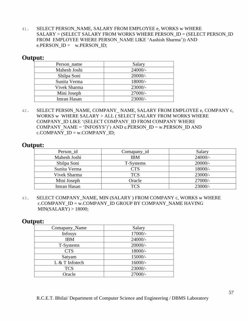
R.C.E.T. Bhilai/ Department of Computer Science and Engineering / DBMS Laboratory
57
41. SELECT PERSON_NAME, SALARY FROM EMPLOYEE e, WORKS w WHERE
SALARY > (SELECT SALARY FROM WORKS WHERE PERSON_ID = (SELECT PERSON_ID
FROM EMPLOYEE WHERE PERSON_NAME LIKE ‗Aashish Sharma‘)) AND
e.PERSON_ID = w.PERSON_ID;
Output: Person_name Salary
Mahesh Joshi 24000/-
Shilpa Soni 20000/-
Sunita Verma 18000/-
Vivek Sharma 23000/-
Mini Joseph 27000/-
Imran Hasan 23000/-
42. SELECT PERS0N_NAME, COMPANY_ NAME, SALARY FROM EMPLOYEE e, COMPANY c,
WORKS w WHERE SALARY > ALL ( SELECT SALARY FROM WORKS WHERE
COMPANY_ID LIKE ‗(SELECT COMPANY_ID FROM COMPANY WHERE
COMPANY_NAME = ‗INFOSYS‘)‘) AND e.PERSON_ID = w.PERSON_ID AND
c.COMPANY_ID = w.COMPANY_ID;
Output: Person_id Comapany_id Salary
Mahesh Joshi IBM 24000/-
Shilpa Soni T-Systems 20000/-
Sunita Verma CTS 18000/-
Vivek Sharma TCS 23000/-
Mini Joseph Oracle 27000/-
Imran Hasan TCS 23000/-
43. SELECT COMPANY_NAME, MIN (SALARY ) FROM COMPANY c, WORKS w WHERE
c.COMPANY_ID = w.COMPANY_ID GROUP BY COMPANY_NAME HAVING
MIN(SALARY) > 18000;
Output: Comapany_Name Salary
Infosys 17000/-
IBM 24000/-
T-Systems 20000/-
CTS 18000/-
Satyam 15000/-
L & T Infotech 16000/-
TCS 23000/-
Oracle 27000/-
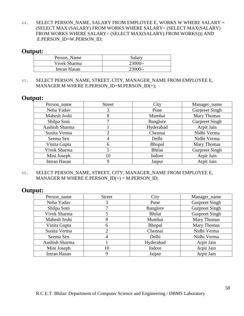
R.C.E.T. Bhilai/ Department of Computer Science and Engineering / DBMS Laboratory
58
44. SELECT PERSON_NAME, SALARY FROM EMPLOYEE E, WORKS W WHERE SALARY =
(SELECT MAX (SALARY) FROM WORKS WHERE SALARY< (SELECT MAX(SALARY)
FROM WORKS WHERE SALARY< (SELECT MAX(SALARY) FROM WORKS))) AND
E.PERSON_ID=W.PERSON_ID;
Output: Person_Name Salary
Vivek Sharma 23000/-
Imran Hasan 23000/-
45. SELECT PERSON_NAME, STREET, CITY, MANAGER_NAME FROM EMPLOYEE E,
MANAGER M WHERE E.PERSON_ID=M.PERSON_ID(+);
Output: Person_name Street City Manager_name
Neha Yadav 3 Pune Gurpreet Singh
Mahesh Joshi 8 Mumbai Mary Thomas
Shilpa Soni 7 Banglore Gurpreet Singh
Aashish Sharma 1 Hyderabad Arpit Jain
Sunita Verma 2 Chennai Nidhi Verma
Seema Sen 4 Delhi Nidhi Verma
Vinita Gupta 6 Bhopal Mary Thomas
Vivek Sharma 5 Bhilai Gurpreet Singh
Mini Joseph 10 Indore Arpit Jain
Imran Hasan 9 Jaipur Arpit Jain
46. SELECT PERSON_NAME, STREET, CITY, MANAGER_NAME FROM EMPLOYEE E,
MANAGER M WHERE E.PERSON_ID(+) = M.PERSON_ID;
Output: Person_name Street City Manager_name
Neha Yadav 3 Pune Gurpreet Singh
Shilpa Soni 7 Banglore Gurpreet Singh
Vivek Sharma 5 Bhilai Gurpreet Singh
Mahesh Joshi 8 Mumbai Mary Thomas
Vinita Gupta 6 Bhopal Mary Thomas
Sunita Verma 2 Chennai Nidhi Verma
Seema Sen 4 Delhi Nidhi Verma
Aashish Sharma 1 Hyderabad Arpit Jain
Mini Joseph 10 Indore Arpit Jain
Imran Hasan 9 Jaipur Arpit Jain
R.C.E.T. Bhilai/ Department of Computer Science and Engineering / DBMS Laboratory
59
Assignment Questions:
a) Find out the products, which have been sold to ‗Ivan Bayross‘.
b) Find out the products and their quantities that will have to be delivered in the current month.
c) Find the products and their quantities for the orders placed by client_no ‗C00001‘ and ‗C00002‘.
Viva-Voce Questions:
1. Explain the difference between ―Where‖ and ―Having‖ Clause.
2. When using the HAVING clause, do you always have to use a GROUP BY also?
3. Why cover outer, inner, left, and right joins when I probably won't ever use them?
4. How many tables can you join on?
5. Would it be fair to say that when tables are joined, they actually become one table?
6. How many rows would a two-table join produce if one table had 50,000 rows and the other had 100,000?
7. What type of join appears in the following SELECT statement? select e.name, e.employee_id, ep.salary
from employee_tbl e,
employee_pay_tbl ep
where e.employee_id = ep.employee_id;
R.C.E.T. Bhilai/ Department of Computer Science and Engineering / DBMS Laboratory
60
Experiment No 11
Aim: Introduction to Views (create, update, drop), sequences (create, alter, drop).
Description:
VIEWS
A view is often referred to as a virtual table. Views are created by using the CREATE VIEW statement.
After the view has been created, you can use the following SQL commands to refer to that view:
SELECT
INSERT
INPUT
UPDATE
DELETE
Views can be created using CREATE VIEW.
The syntax for the CREATE VIEW statement is
Syntax:
CREATE VIEW <view_name> AS
SELECT columnname, columnname
FROM <table_name>
Where columnname = expression list;
Group By grouping criteria
Having predicate
Note: The Order By clause cannot be used while creating a view.
Selecting a data set from the view:
Once a view has been created, it can be queried exactly like a base table.
Syntax:
Select columnname, columnname
From viewname;
Updating views;
Views can also be used for data manipulation(i.e. the user can perform the Insert, Update and Delete
operations).
Views on which data manipulation can be done are called Updatable Views. When you give an updatable
view name in the Update, Insert or Delete SQL statement, modifications to data will be passed to the
underlying table.
R.C.E.T. Bhilai/ Department of Computer Science and Engineering / DBMS Laboratory
61
Views defined from single table
If the user want to Insert records with the help of a view, then the Primary Key column/s and all the NOT
NULL columns must be included in the view.
The user can Update, Delete records with the help of a view even if the Primary Key column and NOT
NULL column/s are excluded from the view definition.
Views defined from multiple tables(Which have no Referencing clause)
In this case even though the Primary Key column/s as well as NOT NULL columns are included in the
View definition the view‘s behavior will be as follows:
The Insert, Update or Delete operation is not allowed. If attempted the Oracle displays an error message.
Views defined from multiple tables(Which have been created with a Referencing clause)
In this case even though the Primary Key and NOT NULL columns are included in the View definition the
view‘s behavior will be as follows:
An Insert operation is not allowed.
The Delete or Modify do not affect the Master Table.
The view can be used to Modify the columns of the detail table included in the view.
If a Delete operation is executed on the view, the corresponding records from the detail table will be
deleted.
Destroying a view:
The drop view command is used to remove a view from the database.
Syntax:
Drop View viewname;
SEQUENCE
Oracle provides an object called a Sequence that can generate numeric values. A sequence can be defined
to:
Generate numbers in ascending or descending order
Provide intervals between numbers.
Caching of sequence numbers in memory to speed up their availability.
CREATE [ TEMPORARY | TEMP ] SEQUENCE seqname [ INCREMENT increment]
[ MINVALUE minvalue ] [ MAXVALUE maxvalue ]
[ START start ] [ CACHE cache ] [ CYCLE ]
Inputs
TEMPORARY or TEMP
If specified, the sequence object is created only for this session, and is automatically dropped on session
exit. Existing permanent sequences with the same name are not visible (in this session) while the temporary
sequence exists, unless they are referenced with schema-qualified names.
seqname
R.C.E.T. Bhilai/ Department of Computer Science and Engineering / DBMS Laboratory
62
The name (optionally schema-qualified) of a sequence to be created.
increment
The INCREMENT increment clause is optional. A positive value will make an ascending sequence, a
negative one a descending sequence. The default value is one (1).
minvalue
The optional clause MINVALUE minvalue determines the minimum value a sequence can generate. The
defaults are 1 and -2^63-1 for ascending and descending sequences, respectively.
maxvalue
The optional clause MAXVALUE maxvalue determines the maximum value for the sequence. The defaults
are 2^63-1 and -1 for ascending and descending sequences, respectively.
start
The optional START start clause enables the sequence to begin anywhere. The default starting value is
minvalue for ascending sequences and maxvalue for descending ones.
cache
The CACHE cache option enables sequence numbers to be preallocated and stored in memory for faster
access. The minimum value is 1 (only one value can be generated at a time, i.e., no cache) and this is also
the default.
CYCLE
The optional CYCLE keyword may be used to enable the sequence to wrap around when the maxvalue or
minvalue has been reached by an ascending or descending sequence respectively. If the limit is reached, the
next number generated will be the minvalue or maxvalue, respectively. Without CYCLE, after the limit is
reached nextval calls will return an error.
Outputs
CREATE SEQUENCE
Message returned if the command is successful.
ERROR: Relation 'seqname' already exists
If the sequence specified already exists.
ERROR: DefineSequence: MINVALUE (start) can't be >= MAXVALUE (max)
If the specified starting value is out of range.
ERROR: DefineSequence: START value (start) can't be < MINVALUE (min)
If the specified starting value is out of range.
ERROR: DefineSequence: MINVALUE (min) can't be >= MAXVALUE (max)
If the minimum and maximum values are inconsistent.
Description CREATE SEQUENCE will enter a new sequence number generator into the current database. This involves
creating and initializing a new single-row table with the name seqname. The generator will be owned by the
user issuing the command.
If a schema name is given then the sequence is created in the specified schema. Otherwise it is created in the
current schema (the one at the front of the search path; see CURRENT_SCHEMA()). TEMP sequences exist
R.C.E.T. Bhilai/ Department of Computer Science and Engineering / DBMS Laboratory
63
in a special schema, so a schema name may not be given when creating a TEMP sequence. The sequence
name must be distinct from the name of any other sequence, table, index, or view in the same schema.
After a sequence is created, you use the functions nextval, currval and setval to operate on the sequence.
These functions are documented in the User's Guide.
Although you cannot update a sequence directly, you can use a query like
SELECT * FROM seqname;
To examine the parameters and current state of a sequence. In particular, the last_value field of the sequence
shows the last value allocated by any backend process.
Assignment Questions:
1. Create a sequence inv_seq with the following parameters, increment by 3, cycle, cache 4 and which will
generate the numbers from 1 to 9999 in ascending order.
2. Create view on OrderNo, OrderDate, OrderStatus of the Sales_Order table table and ProductNo,
ProductRate and QtyOrdered of Sales_Order_Details.
Viva-Voce Questions:
1. Are the following statements true or false?
2. Both views and indexes take up space in the database and therefore must be factored in the planning of
the database size.
3. If someone updates a table on which a view has been created, the view must have an identical update
performed on it to see the same data.
4. Is the following CREATE statement correct?
SQL> create view credit_debts as
(select all from debts
where account_id = 4);
5. Is the following CREATE statement correct?
SQL> create unique view debts as
select * from debts_tbl;
6. Is the following CREATE statement correct?
SQL> drop * from view debts;
7. Is the following CREATE statement correct?
SQL> create index id_index on bills
(account_id);
R.C.E.T. Bhilai/ Department of Computer Science and Engineering / DBMS Laboratory
64
Experiment No 12
Aim: Introduction to Synonyms (create, drop), index(create, drop)
Description:
SYNONYMS
A SYNONYM is an alias for one of the following objects:
table
view
sequence
stored procedure
stored function
package
Syntax:
CREATE SYNONYM <SynonymName> FOR <ObjectName>;
Note:
The Object does not need to exist at the time if its creation.
Synonyms cannot be used in a drop table, drop view or truncate table statements.
Ex:
CREATE TABLE TEST(B NUMBER);
CREATE SYNONYM T FOR TEST;
INSERT INTO T VALUES(4);
INSERT INTO T VALUES(5);
UPDATE T SET a = 40 WHERE a = 4;
DELETE FROM T WHERE a=5;
TRUNCATE TABLE T;
Error: table or view does not exist.
INDEXES
Another way to present data in a different format than it physically exists on the disk is to use an index. In
addition, indexes can also reorder the data stored on the disk (something views cannot do).
Indexes are used in an SQL database for three primary reasons:
To enforce referential integrity constraints by using the UNIQUE keyword
To facilitate the ordering of data based on the contents of the index's field or fields
To optimize the execution speed of queries
When the user fires a Select statement to search for a particular record, the Oracle engine must first locate
the table on the hard disk. The Oracle engine reads system information and locates the starting location of a
R.C.E.T. Bhilai/ Department of Computer Science and Engineering / DBMS Laboratory
65
table‘s record on the current storage media. The Oracle engine then performs a sequential search to locate
records that match user-defined criteria.
Adding indexes to your database enables SQL to use the Direct Access Method. An index is an ordered list
of the contents of a column, (or a group of columns) of a table.Indexing involves forming a two dimensional
Create Index
Indices are created in an existing table to locate rows more quickly and efficiently. It is possible to create an
index on one or more columns of a table, and each index is given a name. The users cannot see the indexes,
they are just used to speed up queries.
Note: Updating a table containing indexes takes more time than updating a table without, this is because the
indexes also need an update. So, it is a good idea to create indexes only on columns that are often used for a
search.
A Unique Index
Creates a unique index on a table. A unique index means that two rows cannot have the same index value.
CREATE UNIQUE INDEX index_name
ON table_name (column_name)
The "column_name" specifies the column you want indexed.
A Simple Index
Creates a simple index on a table. When the UNIQUE keyword is omitted, duplicate values are allowed.
CREATE INDEX index_name
ON table_name (column_name)
The "column_name" specifies the column you want indexed.
Example: This example creates a simple index, named "PersonIndex", on the LastName field of the Person
table:
CREATE INDEX PersonIndex
ON Person (LastName)
If you want to index the values in a column in descending order, you can add the reserved word DESC after
the column name:
CREATE INDEX PersonIndex
ON Person (LastName DESC)
R.C.E.T. Bhilai/ Department of Computer Science and Engineering / DBMS Laboratory
66
If you want to index more than one column you can list the column names within the parentheses, separated
by commas:
CREATE INDEX PersonIndex
ON Person (LastName, FirstName)
Assignment Questions: 1. Create a simple index idx_Prod on product cost price from the Product_Master table.
Viva-Voce Questions: 1. If the data within my table is already in sorted order, why should I use an index on that table?
2. Can I create an index that contains fields from multiple tables?
3. What will happen if a unique index is created on a nonunique field?
4. If you have the disk space and you really want to get your queries smoking, the more indexes the better.
R.C.E.T. Bhilai/ Department of Computer Science and Engineering / DBMS Laboratory
67
Experiment No 13
Aim: Introduction to Data control (grant, revoke).
Description:
Grant
The GRANT command gives specific permissions on an object (table, view, sequence, database, function,
procedural language, or schema) to one or more users or groups of users. These permissions are added to
those already granted, if any.
GRANT { { SELECT | INSERT | UPDATE | DELETE | RULE | REFERENCES | TRIGGER }
[,...] | ALL [ PRIVILEGES ] }
ON [ TABLE ] tablename [, ...]
TO { username | GROUP groupname | PUBLIC } [, ...]
GRANT { { CREATE | TEMPORARY | TEMP } [,...] | ALL [ PRIVILEGES ] }
ON DATABASE dbname [, ...]
TO { username | GROUP groupname | PUBLIC } [, ...]
GRANT { EXECUTE | ALL [ PRIVILEGES ] }
ON FUNCTION funcname ([type, ...]) [, ...]
TO { username | GROUP groupname | PUBLIC } [, ...]
GRANT { USAGE | ALL [ PRIVILEGES ] }
ON LANGUAGE langname [, ...]
TO { username | GROUP groupname | PUBLIC } [, ...]
GRANT { { CREATE | USAGE } [,...] | ALL [ PRIVILEGES ] }
ON SCHEMA schemaname [, ...]
TO { username | GROUP groupname | PUBLIC } [, ...]
The key word PUBLIC indicates that the privileges are to be granted to all users, including those that may
be created later. PUBLIC may be thought of as an implicitly defined group that always includes all users.
Note that any particular user will have the sum of privileges granted directly to him, privileges granted to
any group he is presently a member of, and privileges granted to PUBLIC.
There is no need to grant privileges to the creator of an object, as the creator has all privileges by
default. (The creator could, however, choose to revoke some of his own privileges for safety.) Note that the
ability to grant and revoke privileges is inherent in the creator and cannot be lost. The right to drop an
object, or to alter it in any way not described by a grantable right, is likewise inherent in the creator, and
cannot be granted or revoked.
Depending on the type of object, the initial default privileges may include granting some privileges
to PUBLIC. The default is no public access for tables and schemas; TEMP table creation privilege for
R.C.E.T. Bhilai/ Department of Computer Science and Engineering / DBMS Laboratory
68
databases; EXECUTE privilege for functions; and USAGE privilege for languages. The object creator may
of course revoke these privileges. (For maximum security, issue the REVOKE in the same transaction that
creates the object; then there is no window in which another user may use the object.)
The possible privileges are:
SELECT
Allows SELECT from any column of the specified table, view, or sequence. Also allows the use of COPY
TO. For sequences, this privilege also allows the use of the currval function.
INSERT
Allows INSERT of a new row into the specified table. Also allows COPY FROM.
UPDATE
Allows UPDATE of any column of the specified table. SELECT ... FOR UPDATE also requires this
privilege (besides the SELECT privilege). For sequences, this privilege allows the use of the nextval and
setval functions.
DELETE
Allows DELETE of a row from the specified table.
RULE
Allows the creation of a rule on the table/view. (See CREATE RULE statement.)
REFERENCES
To create a foreign key constraint, it is necessary to have this privilege on both the referencing and
referenced tables.
TRIGGER
Allows the creation of a trigger on the specified table. (See CREATE TRIGGER statement.)
CREATE
For databases, allows new schemas to be created within the database. For schemas, allows new objects to be
created within the schema. To rename an existing object, you must own the object and have this privilege
for the containing schema.
TEMPORARY
TEMP
R.C.E.T. Bhilai/ Department of Computer Science and Engineering / DBMS Laboratory
69
Allows temporary tables to be created while using the database.
EXECUTE
Allows the use of the specified function and the use of any operators that are implemented on top of the
function. This is the only type of privilege that is applicable to functions. (This syntax works for aggregate
functions, as well.)
USAGE
For procedural languages, allows the use of the specified language for the creation of functions in that
language. This is the only type of privilege that is applicable to procedural languages.
For schemas, allows access to objects contained in the specified schema (assuming that the objects' own
privilege requirements are also met). Essentially this allows the grantee to "look up" objects within the
schema.
ALL PRIVILEGES
Grant all of the privileges applicable to the object at once. The PRIVILEGES key word is optional in
PostgreSQL, though it is required by strict SQL.
The privileges required by other commands are listed on the reference page of the respective command.
Revoke
The REVOKE command is used to revoke access privileges.
REVOKE [ GRANT OPTION FOR ] <permission> [ ,...n ] ON
[ OBJECT:: ][ schema_name ]. object_name [ ( column [ ,...n ] ) ]
{ FROM | TO } <database_principal> [ ,...n ]
[ CASCADE ]
[ AS <database_principal> ]
<permission>::=
ALL [ PRIVILEGES ] | permission [ ( column [ ,...n ] ) ]
<database_principal>::=
Database_user
| Database_role
| Application_role
R.C.E.T. Bhilai/ Department of Computer Science and Engineering / DBMS Laboratory
70
| Database_user_mapped_to_Windows_User
| Database_user_mapped_to_Windows_Group
| Database_user_mapped_to_certificate
| Database_user_mapped_to_asymmetric_key
| Database_user_with_no_login
Arguments
permission
Specifies a permission that can be revoked on a schema-contained object. For a list of the permissions, see
the Remarks section later in this topic.
ALL
Revoking ALL does not revoke all possible permissions. Revoking ALL is equivalent to revoking all ANSI-
92 permissions applicable to the specified object. The meaning of ALL varies as follows:
Scalar function permissions: EXECUTE, REFERENCES.
Table-valued function permissions: DELETE, INSERT, REFERENCES, SELECT, UPDATE.
Stored Procedure permissions: EXECUTE.
Table permissions: DELETE, INSERT, REFERENCES, SELECT, UPDATE.
View permissions: DELETE, INSERT, REFERENCES, SELECT, UPDATE.
PRIVILEGES
Included for ANSI-92 compliance. Does not change the behavior of ALL.
column
Specifies the name of a column in a table, view, or table-valued function on which the permission is being
revoked. The parentheses ( ) are required. Only SELECT, REFERENCES, and UPDATE permissions can
be denied on a column. column can be specified in the permissions clause or after the securable name.
ON [ OBJECT:: ] [ schema_name ] . object_name
Specifies the object on which the permission is being revoked. The OBJECT phrase is optional if
schema_name is specified. If the OBJECT phrase is used, the scope qualifier (::) is required. If
schema_name is not specified, the default schema is used. If schema_name is specified, the schema scope
qualifier (.) is required.
R.C.E.T. Bhilai/ Department of Computer Science and Engineering / DBMS Laboratory
71
{ FROM | TO } <database_principal>
Specifies the principal from which the permission is being revoked.
GRANT OPTION
Indicates that the right to grant the specified permission to other principals will be revoked. The permission
itself will not be revoked.
CASCADE
Indicates that the permission being revoked is also revoked from other principals to which it has been
granted or denied by this principal.
AS <database_principal>
Specifies a principal from which the principal executing this query derives its right to revoke the
permission.
Database_user
Specifies a database user.
Database_role
Specifies a database role.
Application_role
Specifies an application role.
Database_user_mapped_to_Windows_User
Specifies a database user mapped to a Windows user.
Database_user_mapped_to_Windows_Group
Specifies a database user mapped to a Windows group.
Database_user_mapped_to_certificate
Specifies a database user mapped to a certificate.
Database_user_mapped_to_asymmetric_key
Specifies a database user mapped to an asymmetric key.
Database_user_with_no_login
Specifies a database user with no corresponding server-level principal.
Remarks
Information about objects is visible in various catalog views.
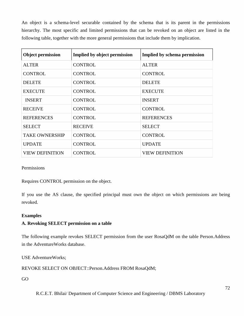
R.C.E.T. Bhilai/ Department of Computer Science and Engineering / DBMS Laboratory
72
An object is a schema-level securable contained by the schema that is its parent in the permissions
hierarchy. The most specific and limited permissions that can be revoked on an object are listed in the
following table, together with the more general permissions that include them by implication.
Object permission Implied by object permission Implied by schema permission
ALTER CONTROL ALTER
CONTROL CONTROL CONTROL
DELETE CONTROL DELETE
EXECUTE CONTROL EXECUTE
INSERT CONTROL INSERT
RECEIVE CONTROL CONTROL
REFERENCES CONTROL REFERENCES
SELECT RECEIVE SELECT
TAKE OWNERSHIP CONTROL CONTROL
UPDATE CONTROL UPDATE
VIEW DEFINITION CONTROL VIEW DEFINITION
Permissions
Requires CONTROL permission on the object.
If you use the AS clause, the specified principal must own the object on which permissions are being
revoked.
Examples
A. Revoking SELECT permission on a table
The following example revokes SELECT permission from the user RosaQdM on the table Person.Address
in the AdventureWorks database.
USE AdventureWorks;
REVOKE SELECT ON OBJECT::Person.Address FROM RosaQdM;
GO
R.C.E.T. Bhilai/ Department of Computer Science and Engineering / DBMS Laboratory
73
B. Revoking EXECUTE permission on a stored procedure
The following example revokes EXECUTE permission on the stored procedure
HumanResources.uspUpdateEmployeeHireInfo from an application role called Recruiting11.
USE AdventureWorks;
REVOKE EXECUTE ON OBJECT::HumanResources.uspUpdateEmployeeHireInfo
FROM Recruiting11;
GO
C. Revoking REFERENCES permission on a view with CASCADE
The following example revokes REFERENCES permission on the column EmployeeID in the view
HumanResources.vEmployee from the user Wanida with CASCADE.
Examples:
Grant insert privilege to all users on table films:
GRANT INSERT ON films TO PUBLIC;
Grant all privileges to user manuel on view kinds:
GRANT ALL PRIVILEGES ON kinds TO manuel;
Assignment Questions:
1. Give the user Sanjay the permission only to view records in the tables Sales_Order and
Sales_Order_Details, along with an option to further grant permission on these tables to other users.
2. Give the user Ashish all data manipulation privileges on the table Client_Master without an option to
further grant permissions on the Client_Master to other users.
3. View the product_no, description of the Product_Master table that belong to Ajay.
4. Take all privileges on the table Client_Master from ashish.
Viva-Voce Questions: 1. The rights that allow the use of some or all of Oracle‘s resources on the Server are called ___________.
2. The __________ statement provides various types of access to database objects.
3. The ____________ privilege allows the grantee to remove records from the table.
4. __________ privilege allow the grantee to query the table.
5. The _____________ allows the grantee to in turn grant object privileges to other users.
6. Privileges once given can be denied to a user using the ______________ command.
7. The Revoke command cannot be used to revoke the privileges granted through the ________.
R.C.E.T. Bhilai/ Department of Computer Science and Engineering / DBMS Laboratory
74
Experiment No 14
Aim: Introduction to PL/SQL
Description:
PL/SQL (Procedural Language/SQL) is a procedural extension of Oracle-SQL that offers language
constructs similar to those in imperative programming languages. PL/SQL allows users and designers to
develop complex database applications that require the usage of control structures and procedural elements
such as procedures, functions, and modules.
Advantages of PL/SQL
These are the advantages of PL/SQL.
Block Structures: PL SQL consists of blocks of code, which can be nested within each other. Each
block forms a unit of a task or a logical module. PL/SQL Blocks can be stored in the database and
reused.
Procedural Language Capability: PL SQL consists of procedural language constructs such as
conditional statements (if else statements) and loops like (FOR loops).
Better Performance: PL SQL engine processes multiple SQL statements simultaneously as a
single block, thereby reducing network traffic.
Error Handling: PL/SQL handles errors or exceptions effectively during the execution of a
PL/SQL program. Once an exception is caught, specific actions can be taken depending upon the
type of the exception or it can be displayed to the user with a message.
The Structure of a PL/SQL Block
PL/SQL is a block-structured language, meaning that PL/SQL programs are divided and written in logical
blocks of code. Within a PL/SQL block of code, processes such as data manipulation or queries can occur.
The following parts of a PL/SQL block are discussed in this section:
The DECLARE section contains the definitions of variables and other objects such as constants and
cursors. This section is an optional part of a PL/SQL block.
The PROCEDURE section contains conditional commands and SQL statements and is where the
block is controlled. This section is the only mandatory part of a PL/SQL block.
The EXCEPTION section tells the PL/SQL block how to handle specified errors and user-defined
exceptions. This section is an optional part of a PL/SQL block.
Here is the basic structure of a PL/SQL block:
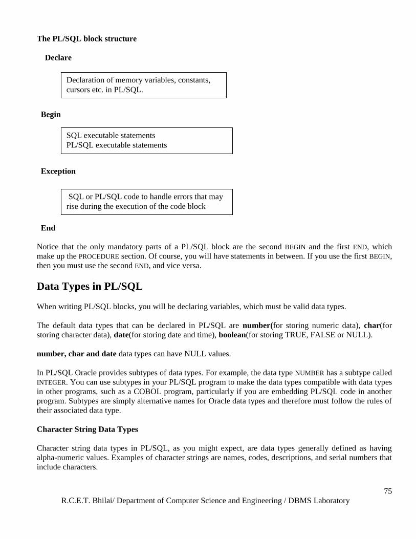
R.C.E.T. Bhilai/ Department of Computer Science and Engineering / DBMS Laboratory
75
The PL/SQL block structure
Declare
Begin
Exception
End
Notice that the only mandatory parts of a PL/SQL block are the second BEGIN and the first END, which
make up the PROCEDURE section. Of course, you will have statements in between. If you use the first BEGIN,
then you must use the second END, and vice versa.
Data Types in PL/SQL
When writing PL/SQL blocks, you will be declaring variables, which must be valid data types.
The default data types that can be declared in PL/SQL are number(for storing numeric data), char(for
storing character data), date(for storing date and time), boolean(for storing TRUE, FALSE or NULL).
number, char and date data types can have NULL values.
In PL/SQL Oracle provides subtypes of data types. For example, the data type NUMBER has a subtype called
INTEGER. You can use subtypes in your PL/SQL program to make the data types compatible with data types
in other programs, such as a COBOL program, particularly if you are embedding PL/SQL code in another
program. Subtypes are simply alternative names for Oracle data types and therefore must follow the rules of
their associated data type.
Character String Data Types
Character string data types in PL/SQL, as you might expect, are data types generally defined as having
alpha-numeric values. Examples of character strings are names, codes, descriptions, and serial numbers that
include characters.
Declaration of memory variables, constants,
cursors etc. in PL/SQL.
SQL executable statements
PL/SQL executable statements
SQL or PL/SQL code to handle errors that may
rise during the execution of the code block
R.C.E.T. Bhilai/ Department of Computer Science and Engineering / DBMS Laboratory
76
CHAR stores fixed-length character strings. The maximum length of CHAR is 32,767 bytes, although it is
hard to imagine a set of fixed-length values in a table being so long.
SYNTAX:
CHAR ( max_length )
Subtype: CHARACTER
VARCHAR2 stores variable-length character strings. You would normally user VARCHAR2 instead of
CHAR to store variable-length data, such as an individual's name. The maximum length of VARCHAR2 is
also 32,767 bytes.
SYNTAX:
VARCHAR2 ( max_length )
Subtypes: VARCHAR, STRING
LONG also stores variable-length character strings, having a maximum length of 32,760 bytes. LONG is
typically used to store lengthy text such as remarks, although VARCHAR2 may be used as well.
Numeric Data Types
NUMBER stores any type of number in an Oracle database.
SYNTAX:
NUMBER ( max_length )
You may specify a NUMBER's data precision with the following syntax:
NUMBER (precision, scale)
Subtypes: DEC, DECIMAL, DOUBLE PRECISION, INTEGER, INT, NUMERIC, REAL, SMALLINT,
FLOAT
PLS_INTEGER defines columns that may contained integers with a sign, such as negative numbers.
Binary Data Types
Binary data types store data that is in a binary format, such as graphics or photographs. These data types
include RAW and LONGRAW.
The DATE Data Type
R.C.E.T. Bhilai/ Department of Computer Science and Engineering / DBMS Laboratory
77
DATE is the valid Oracle data type in which to store dates. When you define a column as a DATE, you do
not specify a length, as the length of a DATE field is implied. The format of an Oracle date is, for example,
01-OCT-97.
BOOLEAN
BOOLEAN stores the following values: TRUE, FALSE, and NULL. Like DATE, BOOLEAN requires no
parameters when defining it as a column's or variable's data type.
ROWID
ROWID is a pseudocolumn that exists in every table in an Oracle database. The ROWID is stored in binary
format and identifies each row in a table. Indexes use ROWIDs as pointers to data.
The %TYPE Attribute
%TYPE declares a variable or constant to have the same data type as that of a previously defined variable or
of a column in a table or view.
NOT NULL
It causes creation of a variable or a constant that cannot be assigned a null value.
For example: Sudent_id number(2) NOT NULL:= '97';
Comments
A comment can have two forms:
SYNTAX:
-- This is a one-line comment.
/* This is a
multiple-line comment.*/
Variable
Variables are values that are subject to change within a PL/SQL block. PL/SQL variables must be assigned
a valid data type upon declaration and can be initialized if necessary. The following example defines a set of
variables in the DECLARE portion of a block:
DECLARE
owner char(10);
tablename char(30);
bytes number(10);
today date;
R.C.E.T. Bhilai/ Department of Computer Science and Engineering / DBMS Laboratory
78
ANALYSIS:
The individual variables are defined on separate lines. Notice that each variable declaration ends with a
semicolon.
Variables may also be initialized in the DECLARE section.
For example:
DECLARE
customer char(30);
fiscal_year number(2):= '97';
You can use the symbol:= to initialize, or assign an initial value, to variables in the DECLARE section. You
must initialize a variable that is defined as NOT NULL.
DECLARE
customer char(30);
fiscal_year number(2) NOT NULL:= '97';
ANALYSIS:
The NOT NULL clause in the definition of fiscal_year resembles a column definition in a CREATE
TABLE statement.
Constant
Constants are defined the same way that variables are, but constant values are static; they do not change. In
the previous example, fiscal_year is probably a constant.
Displaying user messages on the screen
PL/SQL does not provide a direct method for displaying Output as a part of its syntax, but it does allow you
to call a package that serves this function from within the block. The package is called DBMS_OUTPUT.
PUT_LINE expects a single parameter of character data type. If used to display a message, it is the message
string.
To display message, the SERVEROUTPUT should be set to ON.
SERVEROUTPUT is a SQL *PLUS environment parameter that displays the information passed as a
parameter to the PUT_LINE function.
Example:
DBMS_OUTPUT.PUT_LINE( ‗Holiday‘ );
R.C.E.T. Bhilai/ Department of Computer Science and Engineering / DBMS Laboratory
79
Control Flow in PL/SQL
This structure tests a condition, depending on the condition is true or false it decides the sequence of
statements to be executed.
IF...THEN
IF...THEN statement dictates the performance of certain actions if certain conditions are met.
The structure of an IF...THEN statement is as follows:
IF <condition>
THEN <statement_list>
ELSE <statement_list>
END IF;
The ELSE part is optional. If you want a multiway branch, use:
IF <condition_1> THEN ...
ELSIF <condition_2> THEN ...
... ...
ELSIF <condition_n> THEN ...
ELSE ...
END IF;
For example:
Begin
If TO_CHAR( SYSDATE , ‘DY‘ ) = ‘SUN‘ Then
DBMS_OUTPUT.PUT_LINE( ‗Holiday‘ );
End If;
End;
LOOPS
Loops in a PL/SQL block allow statements in the block to be processed continuously for as long as the
specified condition exists.
There are three types of loops:
R.C.E.T. Bhilai/ Department of Computer Science and Engineering / DBMS Laboratory
80
LOOP- END LOOP
LOOP is an infinite loop, most often used to scroll a cursor. To terminate this type of loop, you must specify
when to exit. For example, in scrolling a cursor you would exit the loop after the last row in a cursor has
been processed:
Syntax:
LOOP
Statements
END LOOP;
For example:
BEGIN
LOOP
DBMS_OUTPUT.PUT_LINE (‗Hello‘);
END LOOP;
END;
FOR – LOOP
The FOR – LOOP is used to repeatedly execute a set of statements for certain number of times specified by
a starting number and an ending number. The variable value starts at the starting value given and increments
by 1(default and can not be changed) with each iteration. The iteration stops when the variable value reaches
end value specified.
Syntax:
FOR variable IN [Reverse] start...end
LOOP
Statements
END LOOP;
For example:
Declare
R.C.E.T. Bhilai/ Department of Computer Science and Engineering / DBMS Laboratory
81
n Number;
Begin
For n in 1..5
Loop
DBMS_OUTPUT.PUT_LINE(n);
End Loop;
End;
WHILE-LOOP
This is similar to LOOP. A condition placed between WHILE and LOOP is evaluated before each iteration.
If the condition evaluates to TRUE the statements are executed and the control resumes at the top of the
LOOP. If the condition evaluates to FALSE or NULL then control comes out of the loop.
Syntax:
While <condition>
Loop
<action>
End Loop;
For example:
Declare
n Number:= 1;
Begin
While n<=5
Loop
DBMS_OUPUT.PUT_LINE(n);
n:= n + 1;
End Loop;
R.C.E.T. Bhilai/ Department of Computer Science and Engineering / DBMS Laboratory
82
End;
Sequential Control Statements
The GOTO statement is used for doing unconditional branching to a named label.
Syntax:
GOTO <codeblock name>
For example:
BEGIN
...
GOTO insert_row;
...
<<insert_row>>
INSERT INTO emp VALUES ...
END;
Points To be remembered while working with GOTO:
A statement, at least NULL statement, must follow every GOTO statement
A GOTO statement can branch to enclosing block from the current block
A GOTO statement cannot branch from one IF statement clause to another.
A GOTO statement cannot branch from an enclosing block into a sub-block.
A GOTO statement cannot branch out of a subprogram. A GOTO cannot branch from an exception handler to current block. But it can branch from the exception handler to
an enclosing block
Exception Handling
A PL/SQL block may contain statements that specify exception handling routines. Each error or warning
during the execution of a PL/SQL block raises an exception. One can distinguish between two types of
exceptions:
• System defined exceptions
• User defined exceptions (which must be declared by the user in the declaration part of a block where the
exception is used/implemented)
System defined exceptions are always automatically raised whenever corresponding errors or warnings
occur.
The most common errors that can occur during the execution of PL/SQL programs are handled by system
defined exceptions. The table below lists some of these exceptions with their names and a short description.
R.C.E.T. Bhilai/ Department of Computer Science and Engineering / DBMS Laboratory
83
Error Named Exception Remark
ORA-01001 INVALID_CURSOR Invalid cursor operation such as fetchingfrom a
closed cursor
ORA-01403 NO_DATA_FOUND A select . . . into or fetch statement returned no tuple
ORA-01422 TOO_MANY_ROWS A select . . . into statement returned more than one
tuple
ORA-01476 ZERO_DIVIDE You have tried to divide a number by 0
ORA-06511 CURSOR_ALREADY_OPEN You have tried to open a cursor which is already
open
User Defined Exception Handling
When you declare your own exception, you must raise it explicitly. Exceptions are raised in a block by
using the command RAISE. Exceptions can be raised explicitly by the programmer, whereas internal
database errors are automatically, or implicitly, raised by the database server.
SYNTAX:
BEGIN
DECLARE
exception_name EXCEPTION;
BEGIN
IF condition THEN
RAISE exception_name;
END IF;
EXCEPTION
WHEN exception_name THEN
statement;
END;
END;
ANALYSIS:
This block shows the fundamentals of explicitly raising an exception. First exception_name is declared
using the EXCEPTION statement. In the PROCEDURE section, the exception is raised using RAISE if a given
condition is met. The RAISE then references the EXCEPTION section of the block, where the appropriate
action is taken.
Example:
Declare
emp_sal EMP.SAL%TYPE;
emp_no EMP.EMPNO%TYPE;
R.C.E.T. Bhilai/ Department of Computer Science and Engineering / DBMS Laboratory
84
too high sal exception;
Begin
select EMPNO, SAL into emp_no, emp_sal from EMP where ENAME = ‘KING‘;
if emp_sal * 1.05 > 4000 then raise too high sal
else update EMP set SQL . . .
end if ;
Exception
when NO DATA FOUND – – no tuple selected
then Rollback;
when too high sal then insert into high_sal_emps values(emp no);
Commit;
End;
After the keyword when a list of exception names connected with or can be specified. The last when clause
in the exception part may contain the exception name others. This introduces the default exception handling
routine, for example, a rollback.
All declared exceptions have an error code of 1 and the error message "User-defined exception," unless you
use the EXCEPTION_INIT pragma.
You can associate an error number with a declared exception with the PRAGMA EXCEPTION_INIT
statement:
DECLARE
exception_name EXCEPTION;
PRAGMA EXCEPTION_INIT (exception_name,error_number);
where error_number is a literal value (variable references are not allowed). This number can be an Oracle
error, such as -1855, or an error in the user-definable -20000 to -20999 range.
Transactional Control in PL/SQL
A series of one or more SQL statements that are logically related, or a series of operations performed on
table data is termed as Transaction.
A transaction is a group of events that occurs between any of the following events:
Connecting to Oracle
Disconnecting from oracle
Committing changes to the database table
Rollback
SYNTAX:
BEGIN
DECLARE
...
R.C.E.T. Bhilai/ Department of Computer Science and Engineering / DBMS Laboratory
85
BEGIN
statements...
IF condition THEN
COMMIT;
ELSE
ROLLBACK;
END IF;
...
EXCEPTION
...
END;
END;
Closing Transaction
A trasaction can be closed by using either a Commit or a Rollback statement. By using these statements,
table data can be changed or all the changes made to the table data undone.
COMMIT
The COMMIT statement ends the current transaction and makes permanent any changes made during that
transaction. Until you commit the changes, other users cannot access the changed data; they see the data as
it was before you made the changes.
Syntax:
COMMIT;
Consider a simple transaction that transfers money from one bank account to another. The transaction
requires two updates because it debits the first account, then credits the second. In the example below, after
crediting the second account, you issue a commit, which makes the changes permanent. Only then do other
users see the changes.
BEGIN
...
UPDATE accts SET bal = my_bal - debit
WHERE acctno = 7715;
...
UPDATE accts SET bal = my_bal + credit
WHERE acctno = 7720;
COMMIT;
END;
ROLLBACK
The ROLLBACK statement ends the current transaction and undoes any changes made during that
transaction.
R.C.E.T. Bhilai/ Department of Computer Science and Engineering / DBMS Laboratory
86
Syntax:
ROLLBACK [WORK] [TO SAVEPOINT] savepoint]
Where
WORK: is optional and is provided for ANSI compatibility.
SAVEPOINT: is optional and is used to rollback a partial transaction, as far as the specified savepoint.
savepoint: is a savepoint created during the current transaction.
Example:
Consider the example below, in which you insert information about an employee into three different
database tables. All three tables have a column that holds employee numbers and is constrained by a unique
index. If an INSERT statement tries to store a duplicate employee number, the predefined exception
DUP_VAL_ON_INDEX is raised. In that case, you want to undo all changes, so you issue a rollback in the
exception handler.
DECLARE
emp_id INTEGER;
...
BEGIN
SELECT empno, ... INTO emp_id, ... FROM new_emp WHERE ...
...
INSERT INTO emp VALUES (emp_id, ...);
INSERT INTO tax VALUES (emp_id, ...);
INSERT INTO pay VALUES (emp_id, ...);
...
EXCEPTION
WHEN DUP_VAL_ON_INDEX THEN
ROLLBACK;
...
END;
SAVEPOINT
SAVEPOINT names and marks the current point in the processing of a transaction. Used with the
ROLLBACK TO statement, savepoints let you undo parts of a transaction instead of the whole transaction.
In the example below, you mark a savepoint before doing an insert. If the INSERT statement tries to store a
duplicate value in the empno column, the predefined exception DUP_VAL_ON_INDEX is raised. In that
case, you roll back to the savepoint, undoing just the insert.
DECLARE
emp_id emp.empno%TYPE;
BEGIN
UPDATE emp SET ... WHERE empno = emp_id;
R.C.E.T. Bhilai/ Department of Computer Science and Engineering / DBMS Laboratory
87
DELETE FROM emp WHERE ...
...
SAVEPOINT do_insert;
INSERT INTO emp VALUES (emp_id, ...);
EXCEPTION
WHEN DUP_VAL_ON_INDEX THEN
ROLLBACK TO do_insert;
END;
What are Cursors?
A cursor is a temporary work area created in the system memory when a SQL statement is executed. A
cursor contains information on a select statement and the rows of data accessed by it. This temporary work
area is used to store the data retrieved from the database, and manipulate this data. A cursor can hold more
than one row, but can process only one row at a time. The set of rows the cursor holds is called the active
set.
There are two types of cursors in PL/SQL:
Implicit cursors:
These are created by default when DML statements like, INSERT, UPDATE, and DELETE statements are
executed. They are also created when a SELECT statement that returns just one row is executed.
Explicit cursors:
They must be created when you are executing a SELECT statement that returns more than one row. Even
though the cursor stores multiple records, only one record can be processed at a time, which is called as
current row. When you fetch a row the current row position moves to next row.
Both implicit and explicit cursors have the same functionality, but they differ in the way they are accessed.
Implicit Cursors:
When you execute DML statements like DELETE, INSERT, UPDATE and SELECT statements, implicit
statements are created to process these statements.
Oracle provides few attributes called as implicit cursor attributes to check the status of DML operations.
The cursor attributes available are %FOUND, %NOTFOUND, %ROWCOUNT, and %ISOPEN.
The status of the cursor for each of these attributes are defined in the below table.
Attributes Return Value Example
%FOUND The return value is TRUE, if the DML
statements like INSERT, DELETE and
UPDATE affect at least one row and if
SELECT ….INTO statement return at least one
SQL%FOUND
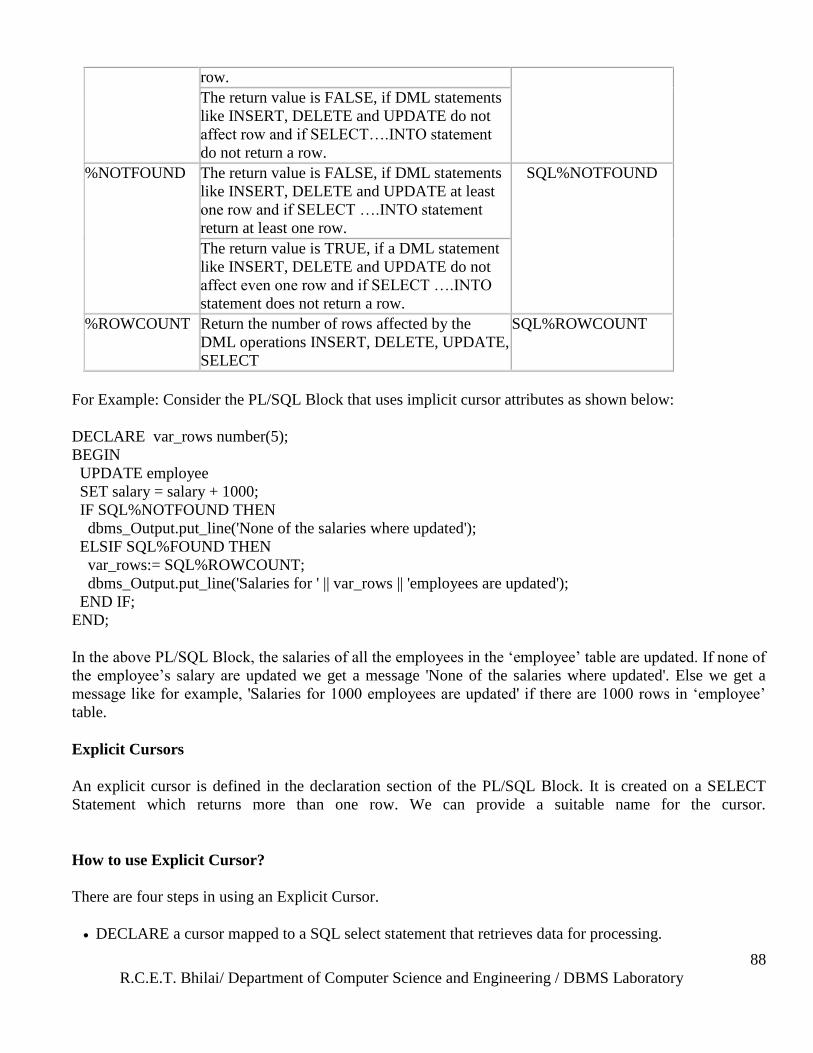
R.C.E.T. Bhilai/ Department of Computer Science and Engineering / DBMS Laboratory
88
row.
The return value is FALSE, if DML statements
like INSERT, DELETE and UPDATE do not
affect row and if SELECT….INTO statement
do not return a row.
%NOTFOUND The return value is FALSE, if DML statements
like INSERT, DELETE and UPDATE at least
one row and if SELECT ….INTO statement
return at least one row.
SQL%NOTFOUND
The return value is TRUE, if a DML statement
like INSERT, DELETE and UPDATE do not
affect even one row and if SELECT ….INTO
statement does not return a row.
%ROWCOUNT Return the number of rows affected by the
DML operations INSERT, DELETE, UPDATE,
SELECT
SQL%ROWCOUNT
For Example: Consider the PL/SQL Block that uses implicit cursor attributes as shown below:
DECLARE var_rows number(5);
BEGIN
UPDATE employee
SET salary = salary + 1000;
IF SQL%NOTFOUND THEN
dbms_Output.put_line('None of the salaries where updated');
ELSIF SQL%FOUND THEN
var_rows:= SQL%ROWCOUNT;
dbms_Output.put_line('Salaries for ' || var_rows || 'employees are updated');
END IF;
END;
In the above PL/SQL Block, the salaries of all the employees in the ‗employee‘ table are updated. If none of
the employee‘s salary are updated we get a message 'None of the salaries where updated'. Else we get a
message like for example, 'Salaries for 1000 employees are updated' if there are 1000 rows in ‗employee‘
table.
Explicit Cursors
An explicit cursor is defined in the declaration section of the PL/SQL Block. It is created on a SELECT
Statement which returns more than one row. We can provide a suitable name for the cursor.
How to use Explicit Cursor?
There are four steps in using an Explicit Cursor.
DECLARE a cursor mapped to a SQL select statement that retrieves data for processing.
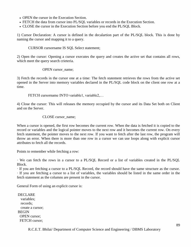
R.C.E.T. Bhilai/ Department of Computer Science and Engineering / DBMS Laboratory
89
OPEN the cursor in the Execution Section.
FETCH the data from cursor into PL/SQL variables or records in the Execution Section.
CLOSE the cursor in the Execution Section before you end the PL/SQL Block.
1) Cursor Declaration: A cursor is defined in the decalartion part of the PL/SQL block. This is done by
naming the cursor and mapping it to a query.
CURSOR cursorname IS SQL Select statement;
2) Open the cursor: Opening a cursor executes the query and creates the active set that contains all rows,
which meet the query search crieteria.
OPEN cursor_name;
3) Fetch the records in the cursor one at a time: The fetch statement retrieves the rows from the active set
opened in the Server into memory variables declared in the PL/SQL code block on the client one row at a
time.
FETCH cursorname INTO variable1, variable2,…
4) Close the cursor: This will releases the memory occupied by the cursor and its Data Set both on Client
and on the Server.
CLOSE cursor_name;
When a cursor is opened, the first row becomes the current row. When the data is fetched it is copied to the
record or variables and the logical pointer moves to the next row and it becomes the current row. On every
fetch statement, the pointer moves to the next row. If you want to fetch after the last row, the program will
throw an error. When there is more than one row in a cursor we can use loops along with explicit cursor
attributes to fetch all the records.
Points to remember while fetching a row:
· We can fetch the rows in a cursor to a PL/SQL Record or a list of variables created in the PL/SQL
Block.
· If you are fetching a cursor to a PL/SQL Record, the record should have the same structure as the cursor.
· If you are fetching a cursor to a list of variables, the variables should be listed in the same order in the
fetch statement as the columns are present in the cursor.
General Form of using an explicit cursor is:
DECLARE
variables;
records;
create a cursor;
BEGIN
OPEN cursor;
FETCH cursor;
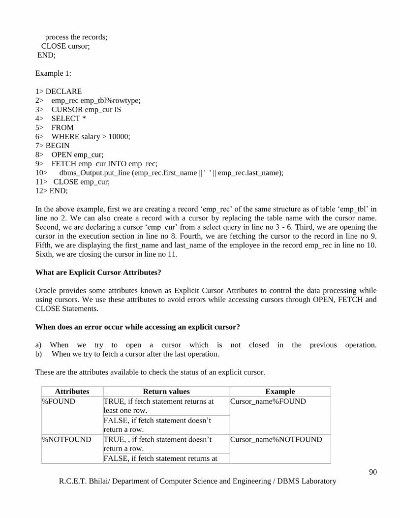
R.C.E.T. Bhilai/ Department of Computer Science and Engineering / DBMS Laboratory
90
process the records;
CLOSE cursor;
END;
Example 1:
1> DECLARE
2> emp_rec emp_tbl%rowtype;
3> CURSOR emp_cur IS
4> SELECT *
5> FROM
6> WHERE salary > 10000;
7> BEGIN
8> OPEN emp_cur;
9> FETCH emp_cur INTO emp_rec;
10> dbms_Output.put_line (emp_rec.first_name || ' ' || emp_rec.last_name);
11> CLOSE emp_cur;
12> END;
In the above example, first we are creating a record ‗emp_rec‘ of the same structure as of table ‗emp_tbl‘ in
line no 2. We can also create a record with a cursor by replacing the table name with the cursor name.
Second, we are declaring a cursor ‗emp_cur‘ from a select query in line no 3 - 6. Third, we are opening the
cursor in the execution section in line no 8. Fourth, we are fetching the cursor to the record in line no 9.
Fifth, we are displaying the first_name and last_name of the employee in the record emp_rec in line no 10.
Sixth, we are closing the cursor in line no 11.
What are Explicit Cursor Attributes?
Oracle provides some attributes known as Explicit Cursor Attributes to control the data processing while
using cursors. We use these attributes to avoid errors while accessing cursors through OPEN, FETCH and
CLOSE Statements.
When does an error occur while accessing an explicit cursor?
a) When we try to open a cursor which is not closed in the previous operation.
b) When we try to fetch a cursor after the last operation.
These are the attributes available to check the status of an explicit cursor.
Attributes Return values Example
%FOUND TRUE, if fetch statement returns at
least one row.
Cursor_name%FOUND
FALSE, if fetch statement doesn‘t
return a row.
%NOTFOUND TRUE, , if fetch statement doesn‘t
return a row.
Cursor_name%NOTFOUND
FALSE, if fetch statement returns at
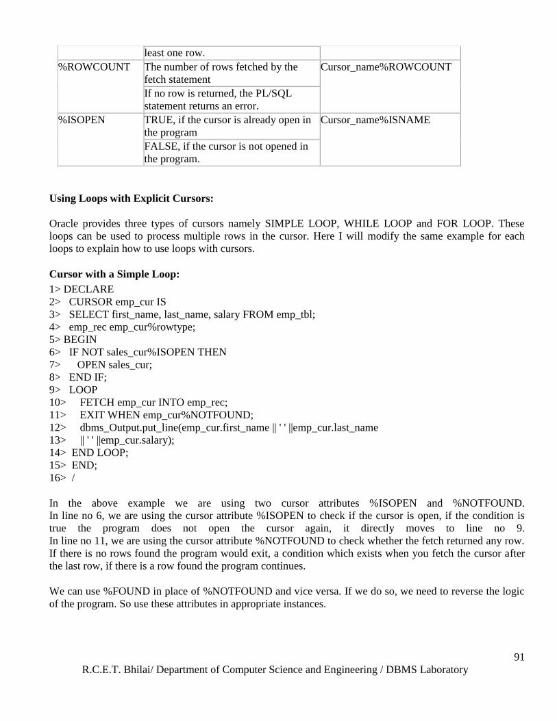
R.C.E.T. Bhilai/ Department of Computer Science and Engineering / DBMS Laboratory
91
least one row.
%ROWCOUNT The number of rows fetched by the
fetch statement
Cursor_name%ROWCOUNT
If no row is returned, the PL/SQL
statement returns an error.
%ISOPEN TRUE, if the cursor is already open in
the program
Cursor_name%ISNAME
FALSE, if the cursor is not opened in
the program.
Using Loops with Explicit Cursors:
Oracle provides three types of cursors namely SIMPLE LOOP, WHILE LOOP and FOR LOOP. These
loops can be used to process multiple rows in the cursor. Here I will modify the same example for each
loops to explain how to use loops with cursors.
Cursor with a Simple Loop:
1> DECLARE
2> CURSOR emp_cur IS
3> SELECT first_name, last_name, salary FROM emp_tbl;
4> emp_rec emp_cur%rowtype;
5> BEGIN
6> IF NOT sales_cur%ISOPEN THEN
7> OPEN sales_cur;
8> END IF;
9> LOOP
10> FETCH emp_cur INTO emp_rec;
11> EXIT WHEN emp_cur%NOTFOUND;
12> dbms_Output.put_line(emp_cur.first_name || ' ' ||emp_cur.last_name
13> || ' ' ||emp_cur.salary);
14> END LOOP;
15> END;
16> /
In the above example we are using two cursor attributes %ISOPEN and %NOTFOUND.
In line no 6, we are using the cursor attribute %ISOPEN to check if the cursor is open, if the condition is
true the program does not open the cursor again, it directly moves to line no 9.
In line no 11, we are using the cursor attribute %NOTFOUND to check whether the fetch returned any row.
If there is no rows found the program would exit, a condition which exists when you fetch the cursor after
the last row, if there is a row found the program continues.
We can use %FOUND in place of %NOTFOUND and vice versa. If we do so, we need to reverse the logic
of the program. So use these attributes in appropriate instances.
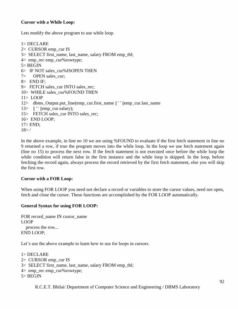
R.C.E.T. Bhilai/ Department of Computer Science and Engineering / DBMS Laboratory
92
Cursor with a While Loop:
Lets modify the above program to use while loop.
1> DECLARE
2> CURSOR emp_cur IS
3> SELECT first_name, last_name, salary FROM emp_tbl;
4> emp_rec emp_cur%rowtype;
5> BEGIN
6> IF NOT sales_cur%ISOPEN THEN
7> OPEN sales_cur;
8> END IF;
9> FETCH sales_cur INTO sales_rec;
10> WHILE sales_cur%FOUND THEN
11> LOOP
12> dbms_Output.put_line(emp_cur.first_name || ' ' ||emp_cur.last_name
13> || ' ' ||emp_cur.salary);
15> FETCH sales_cur INTO sales_rec;
16> END LOOP;
17> END;
18> /
In the above example, in line no 10 we are using %FOUND to evaluate if the first fetch statement in line no
9 returned a row, if true the program moves into the while loop. In the loop we use fetch statement again
(line no 15) to process the next row. If the fetch statement is not executed once before the while loop the
while condition will return false in the first instance and the while loop is skipped. In the loop, before
fetching the record again, always process the record retrieved by the first fetch statement, else you will skip
the first row.
Cursor with a FOR Loop:
When using FOR LOOP you need not declare a record or variables to store the cursor values, need not open,
fetch and close the cursor. These functions are accomplished by the FOR LOOP automatically.
General Syntax for using FOR LOOP:
FOR record_name IN cusror_name
LOOP
process the row...
END LOOP;
Let‘s use the above example to learn how to use for loops in cursors.
1> DECLARE
2> CURSOR emp_cur IS
3> SELECT first_name, last_name, salary FROM emp_tbl;
4> emp_rec emp_cur%rowtype;
5> BEGIN
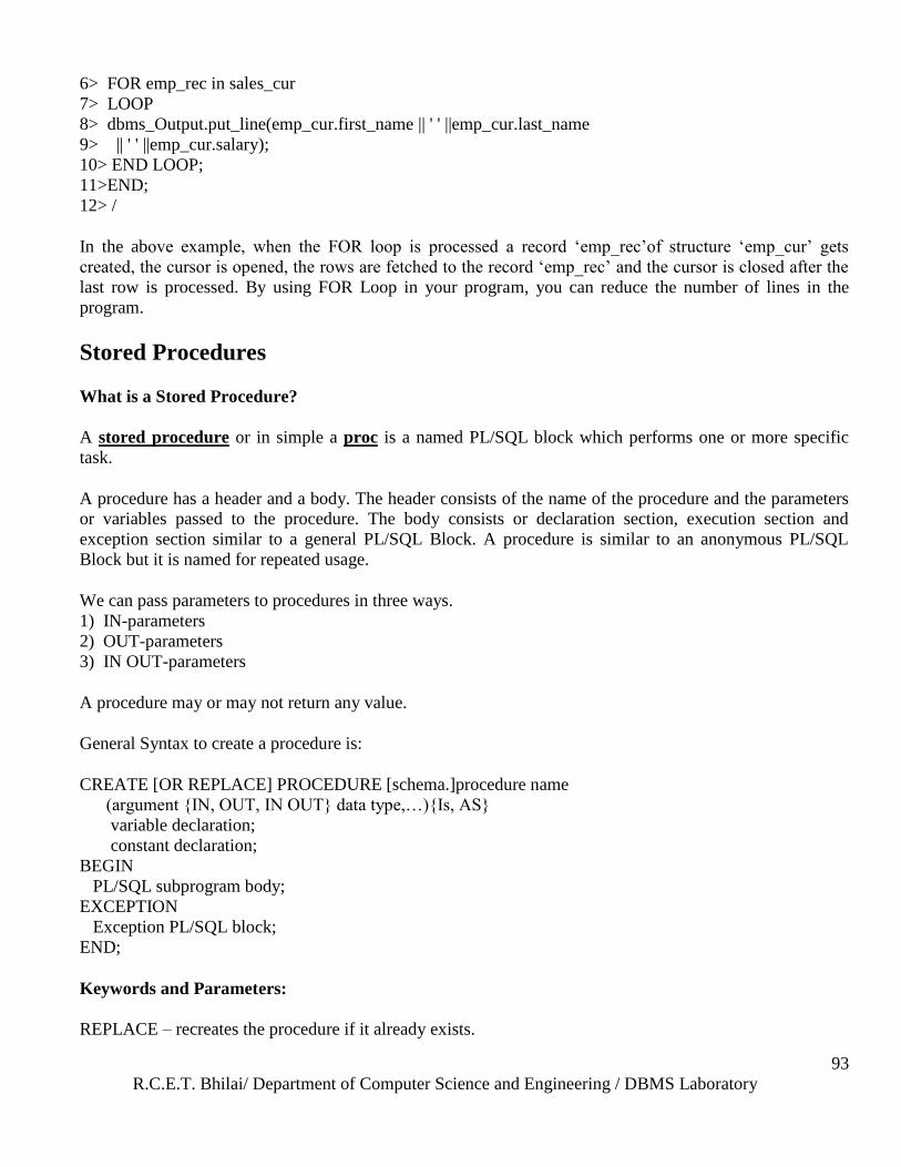
R.C.E.T. Bhilai/ Department of Computer Science and Engineering / DBMS Laboratory
93
6> FOR emp_rec in sales_cur
7> LOOP
8> dbms_Output.put_line(emp_cur.first_name || ' ' ||emp_cur.last_name
9> || ' ' ||emp_cur.salary);
10> END LOOP;
11>END;
12> /
In the above example, when the FOR loop is processed a record ‗emp_rec‘of structure ‗emp_cur‘ gets
created, the cursor is opened, the rows are fetched to the record ‗emp_rec‘ and the cursor is closed after the
last row is processed. By using FOR Loop in your program, you can reduce the number of lines in the
program.
Stored Procedures
What is a Stored Procedure?
A stored procedure or in simple a proc is a named PL/SQL block which performs one or more specific
task.
A procedure has a header and a body. The header consists of the name of the procedure and the parameters
or variables passed to the procedure. The body consists or declaration section, execution section and
exception section similar to a general PL/SQL Block. A procedure is similar to an anonymous PL/SQL
Block but it is named for repeated usage.
We can pass parameters to procedures in three ways.
1) IN-parameters
2) OUT-parameters
3) IN OUT-parameters
A procedure may or may not return any value.
General Syntax to create a procedure is:
CREATE [OR REPLACE] PROCEDURE [schema.]procedure name
(argument {IN, OUT, IN OUT} data type,…){Is, AS}
variable declaration;
constant declaration;
BEGIN
PL/SQL subprogram body;
EXCEPTION
Exception PL/SQL block;
END;
Keywords and Parameters:
REPLACE – recreates the procedure if it already exists.
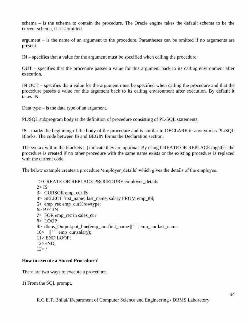
R.C.E.T. Bhilai/ Department of Computer Science and Engineering / DBMS Laboratory
94
schema – is the schema to contain the procedure. The Oracle engine takes the default schema to be the
current schema, if it is omitted.
argument – is the name of an argument to the procedure. Parantheses can be omitted if no arguments are
present.
IN – specifies that a value for the argument must be specified when calling the procedure.
OUT – specifies that the procedure passes a value for this argument back to its calling environment after
execution.
IN OUT – specifies tha a value for the argument must be specified when calling the procedure and that the
procedure passes a value for this argument back to its calling environment after execution. By default it
takes IN.
Data type – is the data type of an argument.
PL/SQL subprogram body is the definition of procedure consisting of PL/SQL statements.
IS - marks the beginning of the body of the procedure and is similar to DECLARE in anonymous PL/SQL
Blocks. The code between IS and BEGIN forms the Declaration section.
The syntax within the brackets [ ] indicate they are optional. By using CREATE OR REPLACE together the
procedure is created if no other procedure with the same name exists or the existing procedure is replaced
with the current code.
The below example creates a procedure ‗employer_details‘ which gives the details of the employee.
1> CREATE OR REPLACE PROCEDURE employer_details
2> IS
3> CURSOR emp_cur IS
4> SELECT first_name, last_name, salary FROM emp_tbl;
5> emp_rec emp_cur%rowtype;
6> BEGIN
7> FOR emp_rec in sales_cur
8> LOOP
9> dbms_Output.put_line(emp_cur.first_name || ' ' ||emp_cur.last_name
10> || ' ' ||emp_cur.salary);
11> END LOOP;
12>END;
13> /
How to execute a Stored Procedure?
There are two ways to execute a procedure.
1) From the SQL prompt.
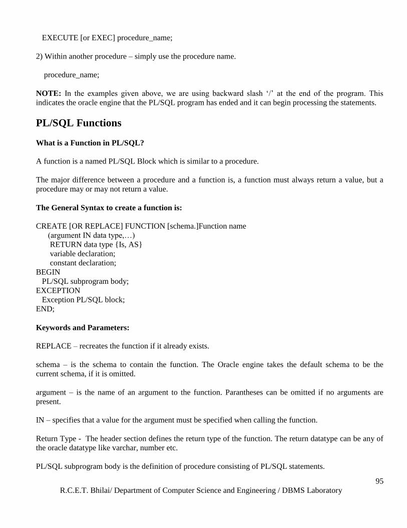
R.C.E.T. Bhilai/ Department of Computer Science and Engineering / DBMS Laboratory
95
EXECUTE [or EXEC] procedure_name;
2) Within another procedure – simply use the procedure name.
procedure_name;
NOTE: In the examples given above, we are using backward slash ‗/‘ at the end of the program. This
indicates the oracle engine that the PL/SQL program has ended and it can begin processing the statements.
PL/SQL Functions
What is a Function in PL/SQL?
A function is a named PL/SQL Block which is similar to a procedure.
The major difference between a procedure and a function is, a function must always return a value, but a
procedure may or may not return a value.
The General Syntax to create a function is:
CREATE [OR REPLACE] FUNCTION [schema.]Function name
(argument IN data type,…)
RETURN data type {Is, AS}
variable declaration;
constant declaration;
BEGIN
PL/SQL subprogram body;
EXCEPTION
Exception PL/SQL block;
END;
Keywords and Parameters:
REPLACE – recreates the function if it already exists.
schema – is the schema to contain the function. The Oracle engine takes the default schema to be the
current schema, if it is omitted.
argument – is the name of an argument to the function. Parantheses can be omitted if no arguments are
present.
IN – specifies that a value for the argument must be specified when calling the function.
Return Type - The header section defines the return type of the function. The return datatype can be any of
the oracle datatype like varchar, number etc.
PL/SQL subprogram body is the definition of procedure consisting of PL/SQL statements.
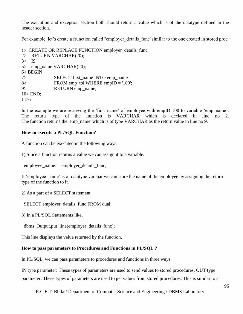
R.C.E.T. Bhilai/ Department of Computer Science and Engineering / DBMS Laboratory
96
The execution and exception section both should return a value which is of the datatype defined in the
header section.
For example, let‘s create a frunction called ''employer_details_func' similar to the one created in stored proc
1> CREATE OR REPLACE FUNCTION employer_details_func
2> RETURN VARCHAR(20);
3> IS
5> emp_name VARCHAR(20);
6> BEGIN
7> SELECT first_name INTO emp_name
8> FROM emp_tbl WHERE empID = '100';
9> RETURN emp_name;
10> END;
11> /
In the example we are retrieving the ‗first_name‘ of employee with empID 100 to variable ‗emp_name‘.
The return type of the function is VARCHAR which is declared in line no 2.
The function returns the 'emp_name' which is of type VARCHAR as the return value in line no 9.
How to execute a PL/SQL Function?
A function can be executed in the following ways.
1) Since a function returns a value we can assign it to a variable.
employee_name:= employer_details_func;
If ‗employee_name‘ is of datatype varchar we can store the name of the employee by assigning the return
type of the function to it.
2) As a part of a SELECT statement
SELECT employer_details_func FROM dual;
3) In a PL/SQL Statements like,
dbms_Output.put_line(employer_details_func);
This line displays the value returned by the function.
How to pass parameters to Procedures and Functions in PL/SQL ?
In PL/SQL, we can pass parameters to procedures and functions in three ways.
IN type parameter: These types of parameters are used to send values to stored procedures. OUT type
parameter: These types of parameters are used to get values from stored procedures. This is similar to a
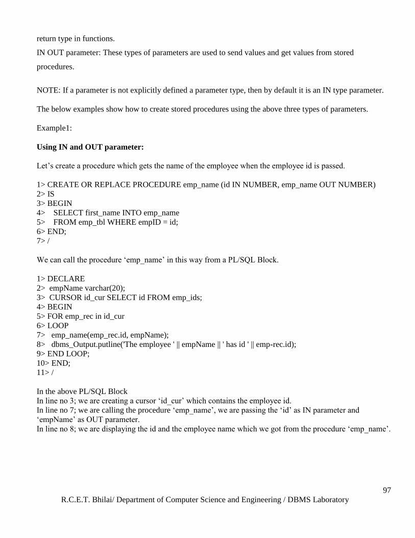
R.C.E.T. Bhilai/ Department of Computer Science and Engineering / DBMS Laboratory
97
return type in functions.
IN OUT parameter: These types of parameters are used to send values and get values from stored
procedures.
NOTE: If a parameter is not explicitly defined a parameter type, then by default it is an IN type parameter.
The below examples show how to create stored procedures using the above three types of parameters.
Example1:
Using IN and OUT parameter:
Let‘s create a procedure which gets the name of the employee when the employee id is passed.
1> CREATE OR REPLACE PROCEDURE emp_name (id IN NUMBER, emp_name OUT NUMBER)
2> IS
3> BEGIN
4> SELECT first_name INTO emp_name
5> FROM emp_tbl WHERE empID = id;
6> END;
7> /
We can call the procedure ‗emp_name‘ in this way from a PL/SQL Block.
1> DECLARE
2> empName varchar(20);
3> CURSOR id_cur SELECT id FROM emp_ids;
4> BEGIN
5> FOR emp_rec in id_cur
6> LOOP
7> emp_name(emp_rec.id, empName);
8> dbms_Output.putline('The employee ' || empName || ' has id ' || emp-rec.id);
9> END LOOP;
10> END;
11> /
In the above PL/SQL Block
In line no 3; we are creating a cursor ‗id_cur‘ which contains the employee id.
In line no 7; we are calling the procedure ‗emp_name‘, we are passing the ‗id‘ as IN parameter and
‗empName‘ as OUT parameter.
In line no 8; we are displaying the id and the employee name which we got from the procedure ‗emp_name‘.
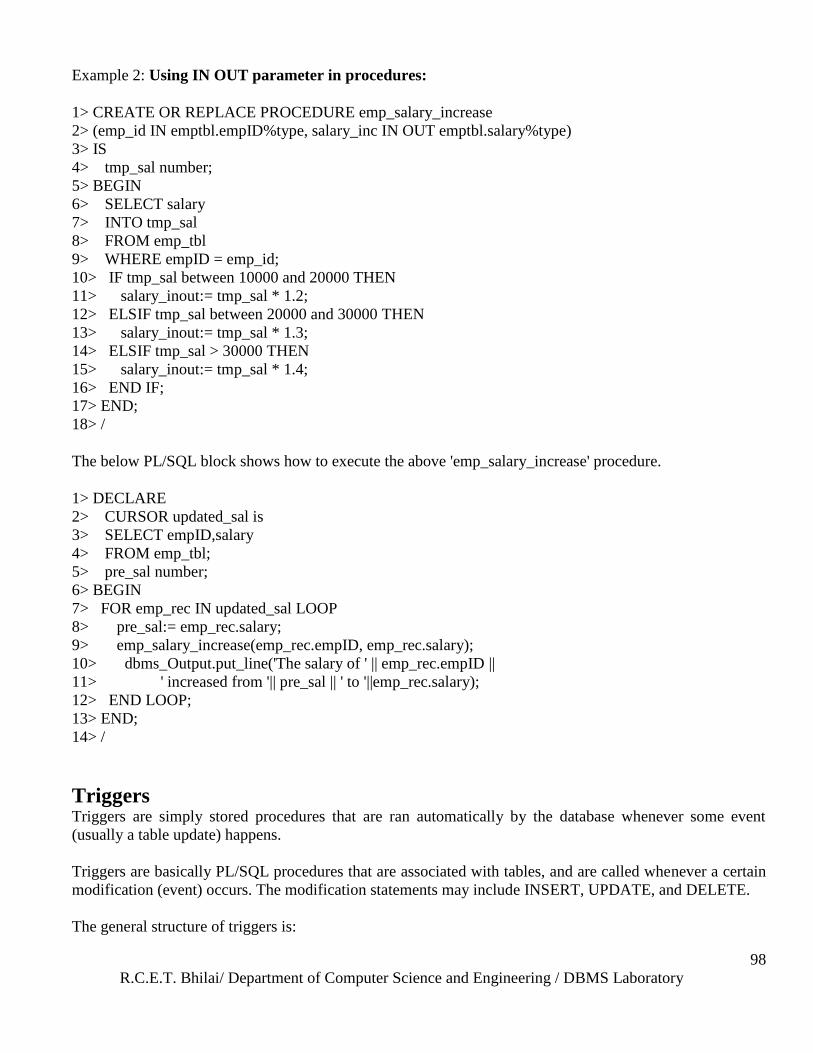
R.C.E.T. Bhilai/ Department of Computer Science and Engineering / DBMS Laboratory
98
Example 2: Using IN OUT parameter in procedures:
1> CREATE OR REPLACE PROCEDURE emp_salary_increase
2> (emp_id IN emptbl.empID%type, salary_inc IN OUT emptbl.salary%type)
3> IS
4> tmp_sal number;
5> BEGIN
6> SELECT salary
7> INTO tmp_sal
8> FROM emp_tbl
9> WHERE empID = emp_id;
10> IF tmp_sal between 10000 and 20000 THEN
11> salary_inout:= tmp_sal * 1.2;
12> ELSIF tmp_sal between 20000 and 30000 THEN
13> salary_inout:= tmp_sal * 1.3;
14> ELSIF tmp_sal > 30000 THEN
15> salary_inout:= tmp_sal * 1.4;
16> END IF;
17> END;
18> /
The below PL/SQL block shows how to execute the above 'emp_salary_increase' procedure.
1> DECLARE
2> CURSOR updated_sal is
3> SELECT empID,salary
4> FROM emp_tbl;
5> pre_sal number;
6> BEGIN
7> FOR emp_rec IN updated_sal LOOP
8> pre_sal:= emp_rec.salary;
9> emp_salary_increase(emp_rec.empID, emp_rec.salary);
10> dbms_Output.put_line('The salary of ' || emp_rec.empID ||
11> ' increased from '|| pre_sal || ' to '||emp_rec.salary);
12> END LOOP;
13> END;
14> /
Triggers Triggers are simply stored procedures that are ran automatically by the database whenever some event
(usually a table update) happens.
Triggers are basically PL/SQL procedures that are associated with tables, and are called whenever a certain
modification (event) occurs. The modification statements may include INSERT, UPDATE, and DELETE.
The general structure of triggers is:
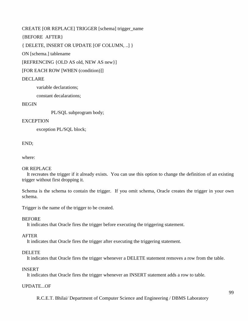
R.C.E.T. Bhilai/ Department of Computer Science and Engineering / DBMS Laboratory
99
CREATE [OR REPLACE] TRIGGER [schema] trigger_name
{BEFORE AFTER}
{ DELETE, INSERT OR UPDATE [OF COLUMN, ..] }
ON [schema.] tablename
[REFRENCING {OLD AS old, NEW AS new}]
[FOR EACH ROW [WHEN (condition)]]
DECLARE
variable declarations;
constant decalarations;
BEGIN
PL/SQL subprogram body;
EXCEPTION
exception PL/SQL block;
END;
where:
OR REPLACE
It recreates the trigger if it already exists. You can use this option to change the definition of an existing
trigger without first dropping it.
Schema is the schema to contain the trigger. If you omit schema, Oracle creates the trigger in your own
schema.
Trigger is the name of the trigger to be created.
BEFORE
It indicates that Oracle fires the trigger before executing the triggering statement.
AFTER
It indicates that Oracle fires the trigger after executing the triggering statement.
DELETE
It indicates that Oracle fires the trigger whenever a DELETE statement removes a row from the table.
INSERT
It indicates that Oracle fires the trigger whenever an INSERT statement adds a row to table.
UPDATE...OF
R.C.E.T. Bhilai/ Department of Computer Science and Engineering / DBMS Laboratory
100
It indicates that Oracle fires the trigger whenever an UPDATE statement changes a value in one of the
columns specified in the OF clause.
If you omit the OF clause, Oracle fires the trigger whenever an UPDATE statement changes a value in any
column of the table.
ON
It specifies the schema and name of the table on which the trigger is to be created. If you omit schema,
Oracle assumes the table is in our own schema. You cannot create a trigger on a table in the schema SYS.
REFERENCING
It specifies correlation names. You can use correlation names in the PL/SQL block and WHEN clause of
a row triggers to refer specifically to old and new values of the current row. The default correlation
names are OLD and NEW. If your row trigger is associated with a table named OLD or NEW, you can use
this clause to specify different correlation names to avoid confusion between the table name and the
correlation name.
FOR EACH ROW
It designates the trigger to be a row trigger. Oracle fires a row trigger once for each row that is affected
by the triggering statement and meets the optional trigger constraint defined in the WHEN clause.
If you omit this clause, the trigger is a statement trigger. Oracle fires a statement trigger only once when
the triggering statement is issued if the optional trigger constraint is met.
WHEN
It specifies the trigger restriction. The trigger restriction contains a SQL condition that must be satisfies
for Oracle to fire the trigger. This condition must contain correlation names and cannot contain a query.
You can only specify a trigger restriction for a row trigger. Oracle evaluates this condition for each row
affected by the triggering statement.
pl/sql_block
It is the PL/SQL block that Oracle executes to fire the trigger.
Example:
Sample Table to be Triggered
Before we begin playing with triggers, let‘s create a simple table with which we can experiment:
CREATE TABLE PERSON (
ID INT,
NAME VARCHAR(30),
DOB DATE,
PRIMARY KEY(ID)
);
The above creates a PERSON table with an ID, a NAME and a DOB columns (fields). Whatever triggers we
define in these notes will relate to this table.
R.C.E.T. Bhilai/ Department of Computer Science and Engineering / DBMS Laboratory
101
Also, let‘s not forget to setup: SET SERVEROUTPUT ON
Before Insert Trigger
Let‘s start out our quest to learn triggers with the simplest case. We have nothing in the database (our
PERSON table is empty). Before we insert any data, we‘d like to perform some operation (let‘s say for
logging purposes, or whatever). We write a trigger to fire before the insert takes place.
CREATE OR REPLACE
TRIGGER PERSON_INSERT_BEFORE
BEFORE
INSERT
ON PERSON
FOR EACH ROW
BEGIN
DBMS_OUTPUT.PUT_LINE(‘BEFORE INSERT OF ‘ ||:NEW.NAME);
END;
Now let us test it out:
INSERT INTO PERSON(ID,NAME,DOB) VALUES (1,‘JOHN DOE‘,SYSDATE);
The single INSERT statement fires the trigger. When we run it, we get the print out of
‘BEFORE INSERT OF JOHN DOE‘.
SQL> INSERT INTO PERSON(ID,NAME,DOB) VALUES (1,‘JOHN DOE‘,SYSDATE);
BEFORE INSERT OF JOHN DOE
1 row created.
Before Update Statement Trigger
Now that we have some data in the table, we can create an update trigger, that would fire whenever
someone tries to update any person (or persons).
CREATE OR REPLACE
TRIGGER PERSON_UPDATE_S_BEFORE
BEFORE UPDATE
ON PERSON
R.C.E.T. Bhilai/ Department of Computer Science and Engineering / DBMS Laboratory
102
BEGIN
DBMS_OUTPUT.PUT_LINE(‘BEFORE UPDATING SOME PERSON(S)‘);
END;
Now, let‘s run an update...
UPDATE PERSON SET DOB = SYSDATE;
Which produces the result:
SQL> UPDATE PERSON SET DOB = SYSDATE;
BEFORE UPDATING SOME PERSON(S)
Trigger Exceptions (introduction)
Triggers become part of the transaction of a statement, which implies that it causes (or raises) any
exceptions (which we‘ll talk about later), the whole statement is rolled back.
For example, to prevent some action that improperly modifies the database. Let‘s say that our database
should not allow anyone to modify their DOB (after the person is in the database, their DOB is assumed to
be static). Anyway, we can create a trigger that would prevent us from updating the DOB:
CREATE OR REPLACE
TRIGGER PERSON_DOB
BEFORE UPDATE OF DOB ON PERSON
FOR EACH ROW
BEGIN
RAISE_APPLICATION_ERROR(-20000,‘CANNOT CHANGE DATE OF BIRTH‘);
END;
Notice the format of the trigger declaration. We explicitly specify that it will be called
BEFORE UPDATE OF DOB ON PERSON.
RAISE_APPLICATION_ERROR
The Oracle engine provides a procedure named RAISE_APPLICATION_ERROR that allows programmers
to issue user-defined error messages.
Syntax:
RAISE_APPLICATION_ERROR(error_number, message);
R.C.E.T. Bhilai/ Department of Computer Science and Engineering / DBMS Laboratory
103
Where,
error_number: is a negative integer in the range -20000 to -20999
message: is a character string up to 2048 bytes in length
The next thing you should notice is the procedure call RAISE_APPLICATION_ERROR, which accepts an
error code, and an explanation string. This effectively halts our trigger execution, and raises an error,
preventing our DOB from being modified. An error (exception) in a trigger stops the code from updating the
DOB.
When we do the actual update for example:
UPDATE PERSON SET DOB = SYSDATE;
We end up with an error, that says we CANNOT CHANGE DATE OF BIRTH.
SQL> UPDATE PERSON SET DOB = SYSDATE;
UPDATE PERSON SET DOB = SYSDATE
*
ERROR at line 1:
ORA-20000: CANNOT CHANGE DATE OF BIRTH
ORA-06512: at "PARTICLE.PERSON_DOB", line 2
ORA-04088: error during execution of trigger ‘PARTICLE.PERSON_DOB‘
You should also notice the error code of ORA-20000. This is our -20000 parameter to RAISE
APPLICATION ERROR.
Viewing Triggers
You can see all your user defined triggers by doing a select statement on USER_TRIGGERS.
For example:
SELECT TRIGGER_NAME FROM USER_TRIGGERS;
Which produces the names of all triggers. You can also select more columns to get more detailed trigger
information.
Dropping Triggers
You can DROP triggers just like anything. The general format would be something like:
DROP TRIGGER trigger_name;
R.C.E.T. Bhilai/ Department of Computer Science and Engineering / DBMS Laboratory
104
Assignment Questions:
1. Create a trigger to restrict insert and update if the entered salary is less than 1000.
2. Create a trigger to display the salary difference when an employee‘s salary is changed.
3. Update the column name, Nmae in Client_Master by adding Mr. to all the names.
4. Write PL/SQL code to display a message when employee with the given employee id does not exist in
employee table.
5. Write down the PL/SQL code to give a salary raise of 5% to all the employees whose salary is greater
than 3000.
6. Write a PL/SQL code block that determines the top three highest paid employees from the Employee
table. Use appropriate cursor attributes for the same. Display the name and the salary of these employees.
Viva-Voce Questions:
1. What is PL/SQL and what is it used for?
2. Can one print to the screen from PL/SQL?
3. What is the difference between Commit and Rollback.
4. What are cursors opened and managed by the Oracle engine.
5. What are the steps to be followed while using Explicit Cursors?
6. Where is the cursor pointer when the cursor is first opened?
7. The data that is stored in a cursor is called ___________
8. Cursors defined by the users are called ______________
9. _____________ is always evaluated to false in case of implicit cursor.
10. What statement/s allow processing of a loop to be aborted?
11. The values that a Boolean variable can take are?
12. What do you mean by exception? Explain.
13. Give some uses of triggers.
14. What is the difference between %TYPE and %ROWTYPE?
15. What is the difference between SQL and PL/SQL?
R.C.E.T. Bhilai/ Department of Computer Science and Engineering / DBMS Laboratory
105
Experiment No 15
Aim: Introduction to ORACLE.
Description:
Every business enterprise maintains large volumes of data for its operations. With more and more people
accessing this data for their work the to maintain its integrity and relevance increases. Normally with
traditional methods of storing data and information in files, the chances that the data loses integrity and
validity are very high.
Oracle is an object relational database management system. It offers capabilities of both relational and
object oriented database systems. In general objects can be defined as reusable software codes which are
location independent and perform a specific task on any application environment with little or no change to
the code.
Oracle products are based on a concept known as client/server technology. This concept involves
segregating the processing of an application between two systems. One performs all activities related to the
database and the other performs activities that help the user to interact with the application.
An Oracle database consists of a collection of data managed by an Oracle database management system.
Popular generic usage also uses the term to refer to the Oracle DBMS management software, but not
necessarily to a specific database under its control.
One can refer to the Oracle database management system unambiguously as Oracle DBMS or (since it
manages databases which have relational characteristics) as Oracle RDBMS.
Oracle Corporation itself blurs the very useful distinction between:
1. data managed by an Oracle RDBMS
2. an Oracle database, and
3. the Oracle RDBMS software itself
When it refers nowadays to the Oracle RDBMS (the software it sells for the purpose of managing databases)
as the Oracle Database. The distinction between the managed data (the database) and the software which
manages the data (the DBMS / RDBMS) relies, in Oracle's marketing literature, on the capitalisation of the
word database.
Oracle Corporation produces and markets the Oracle DBMS, which many database applications use
extensively on many popular computing platforms.
TOOLS OF ORACLE:- The tools provided by oracle are so user friendly that a person with minimum skills in the field of computers
can access them with ease. The main tools are
1. SQL* plus
R.C.E.T. Bhilai/ Department of Computer Science and Engineering / DBMS Laboratory
106
2. PL/SQL
3. isql*plus
SQL stands for structured query language. It is often referred as ―sequel‖. It is originally developed for
IBM‘s DB2 product .It is a nonprocedural language that means SQL describes what data to retrieve, delete
or insert rather than how to perform the operation.
The characteristic that differentiates a DBMS from an RDBMS is that an RDBMS uses a set oriented
database language. For most RDBMS, this set oriented database language is SQL. Set oriented refers to the
way that SQL processes data in sets or groups.
SQL is the de facto standard language used to manipulate and retrieve data from these relational databases.
Through SQL, a programmer can do the following:
1. Modify a databases structure.
2. Change system security settings.
3. Add user permissions to databases or tables.
4. Query a database for information.
5. Updates the concepts of a database.
SQL is basically divided into four parts;
1. DDL
2. DML
3. DCL
4. TCL
DDL stands for data definition language which is to define any table as well as creation of tables. It includes
four basic commands create, drop, alter, truncate.
DML stands for data manipulation language which is used to perform any manipulation, updating the
existing data. We are using four basic commands that are insert, update, select, delete.
TCL stands for transaction control language which is used to control the transactions just performed? In this
we are basically using two commands, ie. Commit and rollback. Commit is used to save the transactions and
rollback is used to unsave the transaction and it backs to its original position.
DCL stands for data control language. It is used to control the data access by the user. If u don‘t want to
give permission to anybody to access any data in that we can. It includes basically two commands that are
grant and revoke.
PL/SQL
It is an extension of SQL. It contain can contain any no. of sql statements integrated with flow of control
statements. It combines the data manipulating power of sql with data processing power of procedural
language.
Architecture Overview
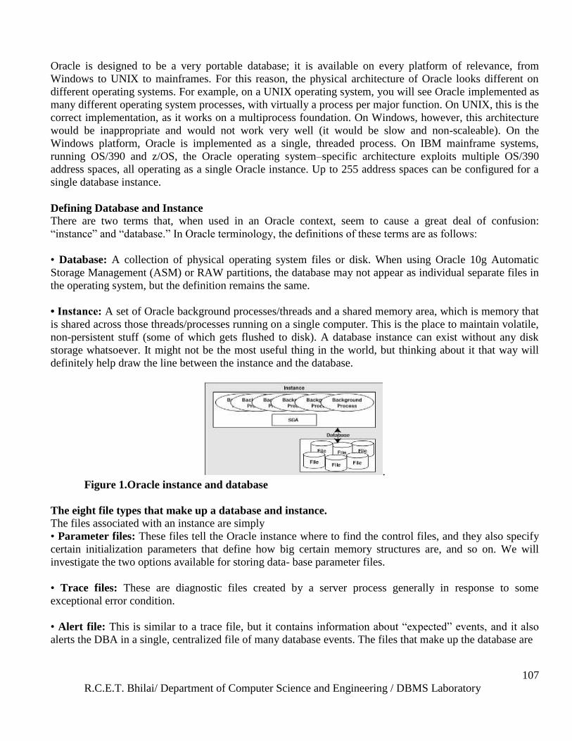
R.C.E.T. Bhilai/ Department of Computer Science and Engineering / DBMS Laboratory
107
Oracle is designed to be a very portable database; it is available on every platform of relevance, from
Windows to UNIX to mainframes. For this reason, the physical architecture of Oracle looks different on
different operating systems. For example, on a UNIX operating system, you will see Oracle implemented as
many different operating system processes, with virtually a process per major function. On UNIX, this is the
correct implementation, as it works on a multiprocess foundation. On Windows, however, this architecture
would be inappropriate and would not work very well (it would be slow and non-scaleable). On the
Windows platform, Oracle is implemented as a single, threaded process. On IBM mainframe systems,
running OS/390 and z/OS, the Oracle operating system–specific architecture exploits multiple OS/390
address spaces, all operating as a single Oracle instance. Up to 255 address spaces can be configured for a
single database instance.
Defining Database and Instance
There are two terms that, when used in an Oracle context, seem to cause a great deal of confusion:
―instance‖ and ―database.‖ In Oracle terminology, the definitions of these terms are as follows:
• Database: A collection of physical operating system files or disk. When using Oracle 10g Automatic
Storage Management (ASM) or RAW partitions, the database may not appear as individual separate files in
the operating system, but the definition remains the same.
• Instance: A set of Oracle background processes/threads and a shared memory area, which is memory that
is shared across those threads/processes running on a single computer. This is the place to maintain volatile,
non-persistent stuff (some of which gets flushed to disk). A database instance can exist without any disk
storage whatsoever. It might not be the most useful thing in the world, but thinking about it that way will
definitely help draw the line between the instance and the database.
.
Figure 1.Oracle instance and database
The eight file types that make up a database and instance.
The files associated with an instance are simply
• Parameter files: These files tell the Oracle instance where to find the control files, and they also specify
certain initialization parameters that define how big certain memory structures are, and so on. We will
investigate the two options available for storing data- base parameter files.
• Trace files: These are diagnostic files created by a server process generally in response to some
exceptional error condition.
• Alert file: This is similar to a trace file, but it contains information about ―expected‖ events, and it also
alerts the DBA in a single, centralized file of many database events. The files that make up the database are
R.C.E.T. Bhilai/ Department of Computer Science and Engineering / DBMS Laboratory
108
• Data files: These files are for the database; they hold your tables, indexes, and all other segments.
• Temp files: These files are used for disk-based sorts and temporary storage.
• Control files: These files tell you where the data files, temp files, and redo log files are, as well as other
relevant metadata about their state.
• Redo log files: These are your transaction logs.
• Password files: These files are used to authenticate users performing administrative
Assignment/Viva-Voce Questions:
1. What is database management system and database system?
2. What are the advantages of RDBMS?
3. What is difference between database and instance?
4. Explain difference between RDBMS and DBMS?
R.C.E.T. Bhilai/ Department of Computer Science and Engineering / DBMS Laboratory
109
Experiment No 16
Aim: Study of Oracle Architectural Components.
Description:
Overview of Primary Components
The Oracle architecture includes a number of primary components, which are discussed further in this
lesson.
Oracle server: There are several files, processes, and memory structures in an Oracle server; however, not
all of them are used when processing a SQL statement. Some are used to improve the performance of the
database, ensure that the database can be recovered in the event of a software or hardware error, or perform
other tasks necessary to maintain the database. The Oracle server consists of an Oracle instance and an
Oracle database.
Oracle instance: An Oracle instance is the combination of the background processes and memory
structures. The instance must be started to access the data in the database. Every time an instance is started,
a System Global Area (SGA) is allocated and Oracle background processes are started. Background
processes perform functions on behalf of the invoking process. They consolidate functions that would
otherwise be handled by multiple Oracle programs running for each user. The background processes
perform input/Output (I/O) and monitor other Oracle processes to provide increased parallelism for better
performance and reliability.
Oracle database: An Oracle database consists of operating system files, also known as database files, that
provide the actual physical storage for database information. The database files are used to ensure that the
data is kept consistent and can be recovered in the event of a failure of the instance.
Other key files: Nondatabase files are used to configure the instance, authenticate privileged users, and
recover the database in the event of a disk failure.
User and server processes: The user and server processes are the primary processes involved when a SQL
statement is executed; however, other processes may help the server complete the processing of the SQL
statement.
Other processes: Many other processes exist that are used by other options within Oracle, such as
Advanced Queuing, Real Application Clusters, Shared Server, Advanced Replication, and so on. These
processes are discussed within their respective courses.
Oracle Server
The Oracle server can run on a number of different computers in one of the following ways:
Client-Application Server-Server
Client-Server
Host-Based
R.C.E.T. Bhilai/ Department of Computer Science and Engineering / DBMS Laboratory
110
Client-Application Server-Server: (Three-tier) Users access the database from their personal computers
(clients) through an application server, which is used for the application‘s processing requirements.
Client-Server: (Two-tier) Users access the database from their personal computer (client) over a network,
and the database sits on a separate computer (server).
Host-Based: Users are connected directly to the same computer on which the database resides.
Oracle Instance An Oracle instance consists of the System Global Area (SGA) memory structure and the background
processes used to manage a database. An instance is identified by using methods specific to each operating
system. The instance can open and use only one database at a time.
Connecting to an Oracle Instance
Before users can submit SQL statements to an Oracle database, they must connect to an instance.
The user starts a tool such as SQL*Plus or runs an application developed using a tool such as Oracle Forms.
This application or tool is executed as a user process.
In the most basic configuration, when a user logs on to the Oracle server, a process is created on the
computer running the Oracle server. This process is called a server process. The server process
communicates with the Oracle instance on behalf of the user process that runs on the client. The server
process executes SQL statements on behalf of the user.
Connection
A connection is a communication pathway between a user process and an Oracle server. A database user can
connect to an Oracle server in one of three ways:
The user logs on to the operating system running the Oracle instance and starts an application or tool that
accesses the database on that system. The communication pathway is established using the interprocess
communication mechanisms available on the host operating system.
The user starts the application or tool on a local computer and connects over a network to the computer
running the Oracle instance. In this configuration, called client-server, network software is used to
communicate between the user and the Oracle server.
In a three-tiered connection, the user‘s computer communicates over the network to an application or a
network server, which is connected through a network to the machine running the Oracle instance. For
example, the user runs a browser on a computer on a network to use an application residing on an NT server
that retrieves data from an Oracle database running on a UNIX host.
Sessions
A session is a specific connection of a user to an Oracle server. The session starts when the user is validated
by the Oracle server, and it ends when the user logs out or when there is an abnormal termination. For a
given database user, many concurrent sessions are possible if the user logs on from many tools, applications,
or terminals at the same time. Except for some specialized database administration tools, starting a database
session requires that the Oracle server be available for use.
An Oracle Database
The general purpose of a database is to store and retrieve related information. An Oracle database has a
logical and a physical structure. The physical structure of the database is the set of operating system files in
the database. An Oracle database consists of three file types.
Data files containing the actual data in the database
Redo logs containing a record of changes made to the database to enable recovery of the data in case of
failures
Control files containing information necessary to maintain and verify database integrity
R.C.E.T. Bhilai/ Department of Computer Science and Engineering / DBMS Laboratory
111
Other Key File Structures The Oracle server also uses other files that are not part of the database:
The parameter file defines the characteristics of an Oracle instance. For example, it contains parameters that
size some of the memory structures in the SGA.
The password file authenticates users privileged to start up and shut down an Oracle instance.Archived redo
log files are offline copies of the redo log files that may be necessary to recover from media failures.
Physical Structure Other key files exist and are required to start up and use a database, for example: parameter files,
configuration files, password files and so on. However, the physical structure of an Oracle database includes
only three types of files: control files, data files, and redo log files.
System Global Area
The SGA is also called the shared global area. It is used to store database information that is shared by
database processes. It contains data and control information for the Oracle server and is allocated in the
virtual memory of the computer where Oracle resides.
Dynamic SGA
A dynamic SGA implements an infrastructure that allows the SGA configuration to change without shutting
down the instance. This then allows the sizes of the database buffer cache, shared pool, and large pool to be
changed without shutting down the instance. Conceivably, the database buffer cache, shared pool, and large
pool could be initially under configured and would grow and shrink depending upon their respective work
loads, up to a maximum of SGA_MAX_SIZE.
Sizing the SGA
The size of the SGA is determined by several initialization parameters. The parameters that most affect
SGA size are:
DB_CACHE_SIZE: The size of the cache of standard blocks.
LOG_BUFFER: The number of bytes allocated for the redo log buffer cache.
SHARED_POOL_SIZE: The size in bytes of the area devoted to shared SQL and PL/SQL.
LARGE_POOL_SIZE: The size of the large pool; the default is zero.
Note: Dynamic SGA and sizing are covered in further detail in the Oracle9i Performance Tuning course.
System Global Area
Unit of Allocation
A granule is a unit of contiguous virtual memory allocation. The size of a granule depends on the
estimated total SGA size whose calculation is based on the value of the parameter SGA_MAX_SIZE.
4 MB if estimated SGA size is < 128 MB
16 MB otherwise
The components (buffer cache, shared pool, and large pool) are allowed to grow and shrink based on
granule boundaries. For each component which owns granules, the number of granules allocated to the
component, any pending operations against the component (e.g., allocation of granules via ALTER
SYSTEM, freeing of granules via ALTER SYSTEM, corresponding self-tuning), and target size in granules
will be tracked and displayed by the V$BUFFER_POOL view. At instance startup, the Oracle server
R.C.E.T. Bhilai/ Department of Computer Science and Engineering / DBMS Laboratory
112
allocates granule entries, one for each granule to support SGA_MAX_SIZE bytes of address space. As
startup continues, each component acquires as many granules as it requires. The minimum SGA
configuration is three granules (one granule for fixed SGA (includes redo buffers; one granule for buffer
cache; one granule for shared pool).
Shared Pool
The shared pool environment contains both fixed and variable structures. The fixed structures remain
relatively the same size, whereas the variable structures grow and shrink based on user and program
requirements. The actual sizing for the fixed and variable structures is based on an initialization parameter
and the work of an Oracle internal algorithm.
Sizing the Shared Pool Since the shared pool is used for objects that can be shared globally, such as reusable SQL execution plans;
PL/SQL packages, procedures, and functions; and cursor information, it must be sized to accommodate the
needs of both the fixed and variable areas. Memory allocation for the shared pool is determined by the
SHARED_POOL_SIZE initialization parameter. It can be dynamically resized using ALTER SYSTEM
SET. After performance analysis, this can be adjusted but the total SGA size cannot exceed
SGA_MAX_SIZE.
Library Cache
The library cache size is based on the sizing defined for the shared pool. Memory is allocated when a
statement is parsed or a program unit is called. If the size of the shared pool is too small, statements are
continually reloaded into the library cache, which affects performance. The library cache is managed by a
least recently used (LRU) algorithm. As the cache fills, less recently used execution paths and parse trees
are removed from the library cache to make room for the new entries. If the SQL or PL/SQL statements are
not reused, they eventually are aged out.
The library cache consists of two structures:
Shared SQL: The Shared SQL stores and shares the execution plan and parse tree for SQL statements run
against the database. The second time that an identical SQL statement is run, it is able to take advantage of
the parse information available in the shared SQL to expedite its execution. To ensure that SQL statements
use a shared SQL area whenever possible, the text, schema, and bind variables must be exactly the same.
Shared PL/SQL: The shared PL/SQL area stores and shares the most recently executed PL/SQL
statements. Parsed and compiled program units and procedures (functions, packages, and triggers) are stored
in this area.
Data Dictionary Cache
The data dictionary cache is also referred to as the dictionary cache or row cache. Caching data dictionary
information into memory improves response time. Information about the database (user account data, data
file names, segment names, extent locations, table descriptions, and user privileges) is stored in the data
dictionary tables. When this information is needed by the database, the data dictionary tables are read, and
the data that is returned is stored in the data dictionary cache.
Sizing the Data Dictionary The overall size is dependent on the size of the shared pool size and is managed internally by the database.
If the data dictionary cache is too small, then the database has to query the data dictionary tables repeatedly
for information needed by the database. These queries are called recursive calls and are slower than the
queries that are handled by the data dictionary cache.
R.C.E.T. Bhilai/ Department of Computer Science and Engineering / DBMS Laboratory
113
Database Buffer Cache
When a query is processed, the Oracle server process looks in the database buffer cache for any blocks it
needs. If the block is not found in the database buffer cache, the server process reads the block from the data
file and places a copy in the database buffer cache. Because subsequent requests for the same block may
find the block in memory, the requests may not require physical reads. The Oracle server uses a least
recently used algorithm to age out buffers that have not been accessed recently to make room for new blocks
in the database buffer cache.
Sizing the Database Buffer Cache
The size of each buffer in the buffer cache is equal to the size of an Oracle block, and it is specified by the
DB_BLOCK_SIZE parameter. The database buffer cache consists of independent sub-caches for buffer
pools and for multiple block sizes. The parameter DB_BLOCK_SIZE determines the primary block size,
which is used for the SYSTEM tablespace.
Three parameters define the sizes of the buffer caches:
DB_CACHE_SIZE: Sizes the default buffer cache size only, it always exists and cannot be set to zero.
DB_KEEP_CACHE_SIZE: Sizes the keep buffer cache, which is used to retain blocks in memory that are
likely to be reused.
DB_RECYCLE_CACHE_SIZE: Sizes the recycle buffer cache, which is used to eliminate blocks from
memory that have little change of being reused.
Multiple Block Sizes
An Oracle database can be created with a standard block size and up to four non-standard block sizes. Non-
standard block sizes can have any power-of-two value between 2 KB and 32 KB.
Note: Multiple block sizing is covered further in the Oracle9i Performance Tuning course.
Buffer Cache Advisory Parameter
The buffer cache advisory feature enables and disables statistics gathering for predicting behavior with
different cache sizes. The information provided by these statistics can help DBA size the buffer cache
optimally for a given workload. The buffer cache advisory information is collected and displayed through
the V$DB_CACHE_ADVICE view.
The buffer cache advisory is enabled via the initialization parameter DB_CACHE_ADVICE. It is a dynamic
parameter via ALTER SYSTEM. Three values (OFF, ON, READY) are available.
DB_CACHE_ADVICE Parameter Values
OFF: Advisory is turned off and the memory for the advisory is not allocated
ON: Advisory is turned on and both cpu and memory overhead is incurred
Attempting to set the parameter to this state when it is in the OFF state may lead to ORA-4031 Inability to
allocate from the shared pool when the parameter is switched to ON. If the parameter is in a READY state it
can be set to ON without error since the memory is already allocated.
READY: Advisory is turned off but the memory for the advisory remains allocated. Allocating the memory
before the advisory is actually turned on will avoid the risk of ORA-4031. If the parameter is switched to
this state from OFF, it is possible than an ORA-4031 will be raised
Note: Resizing the buffer caches dynamically, the database buffer advisory, and the use and interpretation of
the V$DB_CACHE_ADVICE are covered further in the Oracle9i Performance Tuning course
R.C.E.T. Bhilai/ Department of Computer Science and Engineering / DBMS Laboratory
114
Redo Log Buffer Cache
The redo log buffer cache is a circular buffer that contains changes made to data file blocks. This
information is stored in redo entries. Redo entries contain the information necessary to recreate the data
prior to the change made by INSERT, UPDATE, DELETE, CREATE, ALTER, or DROP operations.
Sizing the Redo Log Buffer Cache
The size of the redo log buffer cache is defined by the initialization parameter LOG_BUFFER.
Note: Sizing the Redo Log Buffer Cache is covered in further detail in the Oracle9i Performance Tuning
course. Refer to the Managing Redo Log Files lesson for details regarding redo log files.
Large Pool
When users connect through the shared server, Oracle needs to allocate additional space in the shared pool
for storing information about the connections between the user processes, dispatchers, and servers. The
large pool relieves the burden on areas within the shared pool. The shared pool does not have to give up
memory for caching SQL parse trees in favor of shared server session information, I/O, and backup and
recover processes. The performance gain is from the reduction of overhead from increasing and shrinkage of
the shared SQL cache.
Backup and Restore
Recovery Manager (RMAN) uses the large pool when the BACKUP_DISK_IO= n and
BACKUP_TAPE_IO_SLAVE = TRUE parameters are set. If the large pool is configured but is not large
enough, the allocation of memory from the large pool fails. RMAN writes an error message to the alert log
file and does not use I/O slaves for backup or restore.
Sizing the Large Pool
The large pool is sized in bytes defined by the LARGE_POOL_SIZE parameter.
Java Pool
The Java pool is an optional setting but is required if installing and using Java. Its size is set, in bytes, using
the JAVA_POOL_SIZE parameter. In Oracle9i, the default size of the Java Pool is 24M.
Program Global Area Components
The Program Global Area or Process Global Area (PGA) is a memory region that contains data and control
information for a single server process or a single background process. The PGA is allocated when a process
is created and deallocated when the process is terminated. In contrast to the SGA, which is shared by several
processes, the PGA is an area that is used by only one process. In a dedicated server configuration, the PGA
includes these components:
Sort area: Used for any sorts that may be required to process the SQL statement
Session information: Includes user privileges and performance statistics for the session
Cursor state: Indicates the stage in the processing of the SQL statements that are currently used by the
session
Stack space: Contains other session variables
Note: Some of these structures are stored in the SGA when using a shared server configuration. If using a
shared server configuration, it is possible for multiple user processes to share server processes. If a large
pool is created, the structures are stored in the large pool; otherwise, they are stored in the shared pool.
User Process
A database user who needs to request information from the database must first make a connection with the
Oracle server. The connection is requested using a database interface tool, such as SQL*Plus, and beginning
R.C.E.T. Bhilai/ Department of Computer Science and Engineering / DBMS Laboratory
115
the user process. The user process does not interact directly with the Oracle server. Rather it generates calls
through the user program interface (UPI), which creates a session and starts a server process.
Server Process
Once a user has established a connection, a server process is started to handle the user processes requests. A
server process can be either a dedicated server process or a shared server process. In a dedicated server
environment, the server process handles the request of a single user process. Once a user process
disconnects, the server process is terminated. In a shared server environment, the server process handles the
request of several user processes. The server process communicates with the Oracle server using the Oracle
Program Interface (OPI).
Note: Allocation of server process in a dedicated environment versus a shared environment is covered in
further detail in the Oracle9i Performance Tuning course.
Background Processes
The Oracle architecture has five mandatory background processes that are discussed further in this lesson. In
addition to the mandatory list, Oracle has many optional background process that are started when their
option is being used. These optional processes are not within the scope of this course, with the exception of
the ARCn background process. Following is a list of some optional background processes:
RECO: Recoverer
QMNn: Advanced Queuing
ARCn: Archiver
LCKn: RAC Lock Manager—Instance Locks
LMON: RAC DLM Monitor—Global Locks
LMDn: RAC DLM Monitor—Remote Locks
CJQ0: Snapshot Refresh
Dnnn: Dispatcher
Snnn: Shared Server
Pnnn: Parallel Query Slaves
Database Writer
The server process records changes to rollback and data blocks in the buffer cache. Database Writer
(DBWn) writes the dirty buffers from the database buffer cache to the data files. It ensures that a sufficient
number of free buffers—buffers that can be overwritten when server processes need to read in blocks from
the data files—are available in the database buffer cache. Database performance is improved because server
processes make changes only in the buffer cache.
DBWn defers writing to the data files until one of the following events occurs:
Incremental or normal checkpoint
The number of dirty buffers reaches a threshold value
A process scans a specified number of blocks when scanning for free buffers and cannot fine any.
Timeout occurs.
A ping request in Real Application Clusters environment.
Placing a normal or temporary tablespace offline.
Placing a tablespace in read only mode.
Dropping or Truncating a table.
ALTER TABLESPACE tablespace name BEGIN BACKUP
R.C.E.T. Bhilai/ Department of Computer Science and Engineering / DBMS Laboratory
116
LOG Writer LGWR performs sequential writes from the redo log buffer cache to the redo log file under the following
situations:
When a transaction commits
When the redo log buffer cache is one-third full
When there is more than a megabyte of changes records in the redo log buffer cache
Before DBWn writes modified blocks in the database buffer cache to the data files
Every 3 seconds.
Because the redo is needed for recovery, LGWR confirms the commit only after the redo is written to disk.
LGWR can also call on DBWn to write to the data files.
Note: DBWn does not write to the online redo logs.
Process Monitor
The background process PMON cleans up after failed processes by:
Rolling back the user‘s current transaction
Releasing all currently held table or row locks
Freeing other resources currently reserved by the user
Checkpoint
An event called a checkpoint occurs when the Oracle background process DBWn writes all the modified
database buffers in the SGA, including both committed and uncommitted data, to the data files.
Checkpoints are implemented for the following reasons:
Checkpoints ensure that data blocks in memory that change frequently are written to data files regularly.
Because of the least recently used algorithm of DBWn, a data block that changes frequently might never
qualify as the least recently used block and thus might never be written to disk if checkpoints did not occur.
Because all database changes up to the checkpoint have been recorded in the data files, redo log entries
before the checkpoint no longer need to be applied to the data files if instance recovery is required.
Therefore, checkpoints are useful because they can expedite instance recovery.
At a checkpoint, the following information is written:
Checkpoint number into the data file headers
Checkpoint number, log sequence number, archived log names, and system change numbers into the control
file.
CKPT does not write data blocks to disk or redo blocks to the online redo logs.
Assignment/Viva-Voce Questions:
1. Explain difference between SGA and PGA?
2. Explain the working of redo log files?
3. Explain log switching?
4. Explain checkpoint in contrast to DBWR?
5. Explain the sizing parameter of db block size?
R.C.E.T. Bhilai/ Department of Computer Science and Engineering / DBMS Laboratory
117
Experiment No 17
Aim: Installation and configuration of oracle database using OUI.
Description:
Features of the Oracle Universal Installer
The Java-based Oracle Universal Installer offers an installation solution for all Java-enabled platforms,
allowing for a common installation flow and user experience independent of the platform.
The Universal Installer:
Detects dependencies among components and performs an installation accordingly.
Can be used to point to a URL where a release or staging area was defined and install software
remotely over HTTP.
Can be used to remove products installed. The deinstallation actions are the ―undo‖ of installation
actions.
Maintains an inventory of all the Oracle homes on a target machine, their names, products, and version
of products installed on them.
Detects the language of the operating system and runs the installation session in that language.
Can be run in interactive mode or silent mode. Oracle Universal Installer is run in silent (or non-
interactive) mode using a response file.
Interactive Installation
Unix:
From the top directory of the CD-ROM
$ ./runInstaller
On Unix do not run the Installer as a root user.
Non-Interactive Installation Using Response Files
Non-interactive installation is done when no user action is intended or if non-graphical terminals are used
for installation.
Installation parameters are customized using a response file. Response file is a text file containing variables
and values used by OUI during the installation process. Example of installation parameters include values
for ORACLE_HOME and installation types (i.e., Typical or Custom Install).
The user first needs to edit the response file to specify the components to install. Response file templates are
available in the stage/response directory on Unix platforms. Copy the response files and modify them to suit
your environment.
./runInstaller -responsefile FILENAME [-silent] [-nowelcome]
How to Launch the Oracle Universal Installer in Non-Interactive mode
Example: Launch the Oracle Universal Installer in non-interactive mode.
Unix
./runInstaller –responsefile FILENAME [-SILENT] [-NOWELCOME]
Where: FILENAME: Identifies the response file
SILENT: Runs OUI in silent mode
NOWELCOME: Does not display the Welcome window. If you use
R.C.E.T. Bhilai/ Department of Computer Science and Engineering / DBMS Laboratory
118
SILENT, this parameter is not necessary.
Sample Response File for Unix
[General]
RESPONSEFILE_VERSION=1.0.0.0.0
[Session]
UNIX_GROUP_NAME="dba"
FROM_LOCATION="/u01/stage/products.jar"
ORACLE_HOME="/u01/app/oracle/ora9i"
ORACLE_HOME_NAME="Ora9i"
TOPLEVEL_COMPONENT={"oracle.server", "9.0.1.0.0"}
SHOW_COMPONENT_LOCATIONS_PAGE=false
SHOW_SUMMARY_PAGE=false
SHOW_INSTALL_PROGRESS_PAGE=false
SHOW_REQUIRED_CONFIG_TOOL_PAGE=false
SHOW_OPTIONAL_CONFIG_TOOL_PAGE=false
SHOW_END_SESSION_PAGE=false
NEXT_SESSION=true
SHOW_SPLASH_SCREEN=true
SHOW_WELCOME_PAGE=false
SHOW_ROOTSH_CONFIRMATION=true
SHOW_EXIT_CONFIRMATION=true
INSTALL_TYPE="Typical‖
s_GlobalDBName="u01.us.oracle.com"
s_mountPoint="/u01/app/oracle/ora9i/dbs"
s_dbSid="db09"
b_createDB=true
The General section specifies the version number of the response file
The Sessions section lists various dialogs of the Universal Installer. Some of the dialogs include:
FROM LOCATION specifies the location of the source of the products to be installed
ORACLE_HOME, value for ORACLE_HOME
ORACLE_HOME_NAME, value for ORACLE_HOME_NAME
SHOW INSTALL PROGRESS is the install progress page that appears during the install phase
SHOW ROOTISH CONFIRMATION is set to true if the confirmation dialog to run the root.sh script needs
to be shown
SHOW EXIT CONFIRMATION is set to true if the confirmation when exiting the installer needs to be
shown
Oracle Database Configuration Assistant
Creating a database using Oracle Database Configuration Assistant is covered in lesson Creating a
Database.
Optimal Flexible Architecture (OFA)
Installation and configuration on all supported platforms complies with Optimal Flexible Architecture
(OFA). OFA organizes database files by type and usage. Binary files, control files, log files, and
administrative files can be spread across multiple disks.
Consistent naming convention provides the following benefits:
Database files can be easily differentiated from other files
It is easy to identify control files, redo log files, and data files
R.C.E.T. Bhilai/ Department of Computer Science and Engineering / DBMS Laboratory
119
Easier administration of multiple Oracle Homes on the same machine by separating files on different
disks and directories
Better performance is achieved by decreasing disk contention among data files, binary files, and
administrative files which can now reside on separate directories and disks
Oracle Software Locations
The directory tree above shows an example of OFA-complaint database.
Optimal Flexible Architecture
Another important issue during installation and creation of a database is organizing the file system so that it
is easy to administer growth by adding data into an existing database, adding users, creating new databases,
adding hardware and distributing I/O load across sufficiently many drives.
The Database Administrator Users
Extra privileges are necessary to execute administrative duties on the Oracle server, such as creating users.
Two database user accounts, SYS and SYSTEM, are created automatically with the database and granted
the DBA role. That is, a predefined role that is created automatically with every database. The DBA role has
all database system privileges.
SYS
When a database is created, the user SYS, identified initially by the password change_on_install, is created.
SYS owns the vitally important data dictionary.
SYSTEM
When a database is created, the user SYSTEM, identified initially by the password manager, is also created
automatically. Additional tables and views owned by the user SYSTEM are created. They contain
administrative information used by Oracle tools.
Additional users may be created depending on the mode of database creation i.e., manually, or using
Database Creation Assistant. You will want to create at least one additional administrator username to use
when performing daily administrative tasks.
For security reasons, the default passwords of SYS and SYSTEM should be changed immediately after
database creation.
SQL*Plus
SQL*Plus is Oracle's command line tool to run the standard SQL (Structured Query Language) suite of
commands. SQL is a functional language that users use to communicate with Oracle to retrieve, add, update,
or modify data in the database.
Oracle Enterprise Manager
The Oracle Enterprise Manager is a unified management framework consisting of a Java-based Console, a
suite of tools and services, and a network of management servers and intelligent agents. It includes both
hierarchical tree and graphical representations of the objects and their relationships in the system.
The common services, which include Job Scheduling System, Event Management System,
Repository, Service Discovery, Security, and Paging/Email Blackouts, complete the Oracle Enterprise
Manager framework.
Oracle Enterprise Manager includes integrated applications that allow you to perform both routine and
advanced administration tasks. They include the optional packs such as the Diagnostics Pack, Tuning Pack
and Change Management Pack, and other applications such as Oracle Applications Manager.
R.C.E.T. Bhilai/ Department of Computer Science and Engineering / DBMS Laboratory
120
Note: Optional packs require a separate license.
Oracle Enterprise Manager Architecture
Oracle Enterprise Manager is based on a highly scalable three tier model architecture.
Console
The first tier is comprised of clients such as consoles and management applications, which present graphical
user interfaces to administrators for all management tasks. The first tier depends on the second tier Oracle
Management Server for the bulk of their application logic.
Oracle Management Server
The second tier component of Oracle Enterprise Manager is the Oracle Management Server (OMS). The
OMS is the core of the Enterprise Manager framework and provides administrative user accounts, processes
functions such as jobs, events and manages the flow of information between the Console (first tier) and the
managed nodes (third tier).The OMS uses a repository to store all system data, application data, information
about the state of the managed nodes and information about any system managed packs.
Oracle Enterprise Manager Repository
The Repository is a set of tables, and is created when you set up the OMS. The OMS uses the Oracle
Enterprise Manager repository as its persistent back-end store. If necessary, more than one OMS can be
used. Multiple OMSs share a repository and provide reliability and fault tolerance.
Nodes
The third tier is comprised of managed nodes which contains targets such as databases and other managed
services. Residing on each node is an Oracle Intelligent Agent, which communicates with the OMSs and
performs tasks sent by consoles and client applications.
Only one Intelligent Agent is required per node.
Intelligent Agent functions independently of the database as well as the Console and Management Server.
By running independently of other components, Intelligent Agents can perform such tasks as starting up and
shutting down a database and staying operational if another part of the system is down.
Console Features
The Console provides a graphical interface for administrators and a central launching point for all
applications. Applications such as Instance Manager, Schema Manager, Storage Manager, SQL*Plus
Worksheet can be launched from the Console.
The Console can be run either in thin mode via the web or as a fat client. Thin clients use a web browser to
connect to a server where Console files are installed, whereas fat clients require Console files to be installed
locally. The Console can be launched either in standalone mode or by connecting to Oracle Management
Server.
How to Launch the Oracle Enterprise Manager Console
1. Example: Launch the console and add a database to it.
2. Launch the console: % oemapp console
3. At the Login dialog box choose to launch the application in standalone mode
4. Add Databases to tree: The Add Database to Tree dialog allows you to either add a database
manually by supplying the Hostname, Port number, SID and Net Service name or add selected
databases from your local tnsnames.ora file.
5. Select Add Database To Tree from the Navigator menu
R.C.E.T. Bhilai/ Department of Computer Science and Engineering / DBMS Laboratory
121
6. Enter values for Hostname, SID, Port number and Net Service name
7. Expand your working database from the databases folder
8. Right click your working database and select Connect
9. Enter the username, password and service name for the database and click OK.
Initialization Parameter Files
To start an instance, the Oracle server must read the initialization parameter file.
Initialization Parameter Files
To start an instance, the Oracle server reads the initialization parameter file. Two types of initialization
parameter files exist:
Static parameter file, PFILE, commonly referred to as initSID.ora
Persistent parameter file, SPFILE, commonly referred to as spfileSID.ora
Oracle Managed Files
Oracle Managed Files (OMF) simplify file administration by eliminating the need to directly manage the
files within an Oracle database.
For example: On Solaris, OMF files are named as follows:
Control files: ora_%u.ctl
Redo log files: ora_%g_%u.log
Data files: ora_%t_%u.dbf
Temporary data files: ora_%t_%u.tmp
The following characters are defined as:
%u is an 8-character string that guarantees uniqueness.
%t is the tablespace name, truncated if necessary to fit into the maximum length file name. Placing the
tablespace name before the uniqueness string means that all the data files for a tablespace appear next to
each other in an alphabetic file listing.
%g is the redo log file group number.
ora_ identifies the file as an Oracle Managed File.
Undo files do not have a special extension. As with temporary files, they are considered to be just like any
other data files.
The parameters DB_CREATE_FILE_DEST and DB_CREATE_ONLINE_LOG_DEST_N do not both have
to be set, one or the other or both can be used.
OMF Example
The DB_CREATE_FILE_DEST parameter sets the default file system directory for the data files
(/u01/oradata).
The DB_CREATE_ONLINE_LOG_DEST_1 and DB_CREATE_ONLINE_LOG_DEST_2 parameters set
the default file system directories for online redo log and control file creation. Each online redo log and
control file is multiplexed across the two directories, /u02/oradata and /u03/oradata.
After the initialization parameters are set, the database can be created using the CREATE DATABASE
command. If the command fails, any OMF files created are removed. The internally generated file names
can be seen when the user selects from DBA_DATAFILES and V$LOGFILE.
Both DB_CREATE_FILE_DEST and DB_CREATE_ONLINE_LOG_DEST_N can be modified
dynamically with the ALTER SYSTEM SET command.
R.C.E.T. Bhilai/ Department of Computer Science and Engineering / DBMS Laboratory
122
Starting Up a Database
When starting the database, you select the state in which it starts. The following scenarios describe different
stages of starting up an instance.
Starting the Instance (NOMOUNT) Usually you would start an instance without mounting a database only during database creation or the re-
creation of control files.
Starting an instance includes the following tasks:
Reading the initialization file from $ORACLE_HOME/dbs in the following order:
First spfileSID.ora. If not found then
spfile.ora
initSID.ora
Specifying the PFILE parameter with STARTUP overrides the default behavior
Allocating the SGA
Starting the background processes
Opening the alertSID.log file and the trace files
The database must be named with the DB_NAME parameter either in the initialization file or in the
STARTUP command.
Starting Up a Database
Mounting the Database To perform specific maintenance operations, you start an instance and mount a
database but do not open the database.
For example, the database must be mounted but not open during the following tasks:
Renaming data files
Enabling and disabling redo log archiving options
Performing full database recovery
Mounting a database includes the following tasks:
Associating a database with a previously started instance
Locating and opening the control files specified in the parameter file
Reading the control files to obtain the names and status of the datafiles and redo log files. (However, no
checks are performed to verify the existence of the data files and online redo log files at this time.)
Starting Up a Database
Opening the Database Normal database operation means that an instance is started and the database is
mounted and open; with normal database operation, any valid user can connect to the database and perform
typical data access operations.
Opening the database includes the following tasks:
Opening the online data files
Opening the online redo log files
If any of the data files or online redo log files are not present when you attempt to open the database, the
Oracle server returns an error.
During this final stage, the Oracle server verifies that all the data files and online redo log files can be
opened and checks the consistency of the database. If necessary, the System Monitor background process
(SMON) initiates instance recovery.
Starting Up
To start up an instance, use the following command:
STARTUP [FORCE] [RESTRICT] [PFILE=filename]
R.C.E.T. Bhilai/ Department of Computer Science and Engineering / DBMS Laboratory
123
[OPEN [RECOVER][database]
|MOUNT
|NOMOUNT]
Note: This is not the complete syntax.
where:
OPEN enables users to access the database
MOUNT mounts the database for certain DBA activities but does not provide user access to the database
NOMOUNT creates the SGA and starts up the background processes but does not provide access to the
database
PFILE=parfile enables a nondefault parameter file to be used to configure the instance
FORCE aborts the running instance before performing a normal startup
RESTRICT enables only users with RESTRICTED SESSION privilege to access the database
RECOVER begins media recovery when the database starts
Initialization Parameter File
By default, when the database is started, the Oracle server looks in $ORACLE_HOME/dbs for an
initialization parameter file. The Oracle server first attempts to read file spfilesid.ora and if not found then
file initsid.ora. If neither file is located, an error message is received.
Automating Database Startup
On Unix Automating database startup and shutdown can be controlled by the entries in a special operating
system file; for example, oratab in the /var/opt/oracle directory. Note: Refer to the installation guide for
your operating system for more information.
Troubleshooting Attempting to start the Oracle Utilities without starting these services results in the following error message:
ORA-12547: TNS: lost contact
Changing the Status of the Database
To open the database from STARTUP NOMOUNT to a MOUNT stage or from MOUNT to an OPEN stage,
use the ALTER DATABASE command:
ALTER DATABASE { MOUNT | OPEN }
To prevent data from being modified by user transactions, the database can be opened in read-only mode.
To start up an instance, use the following command:
ALTER DATABASE OPEN [READ WRITE| READ ONLY]
where:
READ WRITE opens the database in read-write mode, so that users can generate redo logs
READ ONLY restricts users to read-only transactions, preventing them from generating redo log
information
Opening a Database in Restricted Mode
A restricted session is useful, for example, when you perform structure maintenance or a database export
and import. The database can be started in restricted mode so that it is available only to users with the
R.C.E.T. Bhilai/ Department of Computer Science and Engineering / DBMS Laboratory
124
RESTRICTED SESSION privilege. The database can also be put in restricted mode by using the ALTER
SYSTEM SQL command:
ALTER SYSTEM [ {ENABLE|DISABLE} RESTRICTED SESSION ]
where:
ENABLE RESTRICTED SESSION: enables future logins only for users who have the RESTRICTED
SESSION privilege
DISABLE RESTRICTED SESSION: disables RESTRICTED SESSION so that users who do not have the
privilege can log on
Terminate Sessions
After placing an instance in restricted mode, you may want to kill all current user sessions before
performing administrative tasks. This can be done by the following:
ALTER SYSTEM KILL SESSION 'integer1,integer2'
where:
integer1: is the value of the SID column in the V$SESSION view
integer2: is the value of the SERIAL# column in the V$SESSION view
Note: The session ID and serial number are used to uniquely identify a session. This guarantees that the
ALTER SYSTEM KILL SESSION command is applied to the correct session even if the user logs off and a
new session uses the same session ID.
Effects of Terminating a Session
The ALTER SYSTEM KILL SESSION command causes the background process PMON to perform the
following steps upon execution:
Roll back the user‘s current transaction
Release all currently held table or row locks
Free all resources currently reserved by the user
Shutting Down the Database
Shut down the database to make operating system offline backups of all physical structures and to have
modified static initialization parameters take effect.
To shut down an instance you must connect as SYSOPER or SYSDBA and use the following command:
SHUTDOWN [NORMAL | TRANSACTIONAL | IMMEDIATE | ABORT ]
Shutdown Options
Shutdown Normal
Normal is the default shutdown mode. Normal database shutdown proceeds with the following conditions:
No new connections can be made.
The Oracle server waits for all users to disconnect before completing the shutdown.
Database and redo buffers are written to disk.
Background processes are terminated, and the SGA is removed from memory.
Oracle closes and dismounts the database before shutting down the instance.
The next startup does not require an instance recovery.
R.C.E.T. Bhilai/ Department of Computer Science and Engineering / DBMS Laboratory
125
Shutdown Transactional
A transactional shutdown prevents clients from losing work. A transactional database shutdown proceeds
with the following conditions:
No client can start a new transaction on this particular instance.
A client is disconnected when the client ends the transaction that is in progress.
When all transactions have finished, a shutdown immediately occurs.
The next startup does not require an instance recovery.
Shutdown Immediate
Immediate database shutdown proceeds with the following conditions:
Current SQL statements being processed by Oracle are not completed.
The Oracle server does not wait for users currently connected to the database to disconnect.
Oracle rolls back active transactions and disconnects all connected users.
Oracle closes and dismounts the database before shutting down the instance.
The next startup does not require an instance recovery.
Shutdown Abort
If the normal and immediate shutdown options do not work, you can abort the current database instance.
Aborting an instance proceeds with the following conditions:
Current SQL statements being processed by the Oracle server are immediately terminated.
Oracle does not wait for users currently connected to the database to disconnect.
Database and redo buffers are not written to disk.
Uncommitted transactions are not rolled back.
The instance is terminated without closing the files.
The database is not closed or dismounted.
The next startup requires instance recovery, which occurs automatically.
Assignment/Viva-Voce Questions:
1. Explain the difference between pfile and spfile?
2. Explain the parameters involved with pfile?
3. How spfile is created with help of pfile?
4. Explain different ways of shutting down database?
5. Explain startup of database using OMF?
6. Explain the status of database in read only mode?
7. Explain how OEM can be used to configure the database?
R.C.E.T. Bhilai/ Department of Computer Science and Engineering / DBMS Laboratory
126
Experiment No 18
Aim: Managing Tablespace and datafiles in oracle database.
Description:
Overview A small database might need only the SYSTEM tablespace; however, Oracle recommends that you create
additional tablespaces to store user data, user indexes, undo segments, and temporary segments separate
from data dictionary. This gives you more flexibility in various database administration operations and
reduces contention among dictionary objects and schema objects for the same data files.
The DBA can create new tablespaces, resize data files, add data files to tablespaces, set and alter default
segment storage settings for segments created in a tablespace, make a tablespace read-only or read-write,
make a tablespace temporary or permanent, and drop tablespaces.
Database Architecture
The Oracle database architecture includes logical and physical structures that make up the database.
The physical structure includes the control files, online redo log files, and data files that make up the
database.
The logical structure includes tablespaces, segments, extents, and data blocks.
The Oracle server enables fine-grained control of disk space use through tablespace and logical storage
structures, including segments, extents, and data blocks.
Tablespaces
The data in an Oracle database are stored in tablespaces.
An Oracle database can be logically grouped into smaller logical areas of space known as tablespaces.
A tablespace can belong to only one database at a time.
Each tablespace consists of one or more operating system files, which are called data files.
A tablespace may consist of zero or more segments.
Tablespaces can be brought online while the database is running.
Except for the SYSTEM tablespace or a tablespace with an active undo segment, tablespaces can be
taken offline, leaving the database running.
Tablespaces can be switched between read-write and read-only status.
Data Files
Each tablespace in an Oracle database consists of one or more files called data files. These are physical
structures that conform with the operating system on which the Oracle server is running.
A data file can belong to only one tablespace.
An Oracle server creates a data file for a tablespace by allocating the specified amount of disk space plus
a small amount of overhead.
The database administrator can change the size of a data file after its creation or can specify that a data
file should dynamically grow as objects in the tablespace grow.
Segments
A segment is the space allocated for a specific logical storage structure within a tablespace. For
example, all of the storage allocated to a table is a segment.
A tablespace may consist of one or more segments.
R.C.E.T. Bhilai/ Department of Computer Science and Engineering / DBMS Laboratory
127
A segment cannot span tablespaces; however, a segment can span multiple data files that belong to the
same tablespace.
Each segment is made up of one or more extents.
Extents
Space is allocated to a segment by extents.
One or more extents make up a segment.
When a segment is created, it consists of at least one extent.
As the segment grows, extents get added to the segment.
The DBA can manually add extents to a segment.
An extent is a set of contiguous Oracle blocks.
An extent cannot span a data file but must exist in one data file.
Data Blocks
The Oracle server manages the storage space in the data files in units called Oracle blocks or data blocks. At
the finest level of granularity, the data in an Oracle database is stored in data blocks. Oracle data blocks are
the smallest units of storage that the Oracle server can allocate, read, or write. One data block corresponds
to one or more operating system blocks allocated from an existing data file. The standard data block size for
an Oracle database is specified by the DB_BLOCK_SIZE initialization parameter when the database is
created. The data block size should be a multiple of the operating system block size to avoid unnecessary
I/O. The maximum data block size is dependent on the operating system.
Types of Tablespaces
The DBA creates tablespaces for increased control and ease of maintenance. The Oracle server perceives
two types of tablespaces: SYSTEM and all others.
SYSTEM Tablespace
Created with the database
Required in all databases
Contains the data dictionary, including stored program units
Contains the SYSTEM undo segment
Should not contain user data, although it is allowed
Non-SYSTEM Tablespaces
Enable more flexibility in database administration
Separate undo, temporary, application data, and application index segments
Separate data by backup requirements
Separate dynamic and static data
Control the amount of space allocated to user‘s objects
CREATE TABLESPACE Command
You create a tablespace with the CREATE TABLESPACE command:
CREATE TABLESPACE tablespace
[DATAFILE clause]
[MINIMUM EXTENT integer[K|M]]
[BLOCKSIZE integer [K]]
[LOGGING|NOLOGGING]
[DEFAULT storage_clause ]
[ONLINE|OFFLINE]
R.C.E.T. Bhilai/ Department of Computer Science and Engineering / DBMS Laboratory
128
[PERMANENT|TEMPORARY]
where:
tablespace is the name of the tablespace to be created
DATAFILE specifies the data file or data files that make up the tablespace.
MINIMUM EXTENT ensures that every used extent size in the tablespace is a multiple of the integer. Use
Kor M to specify this size in kilobytes or megabytes.
LOGGING specifies that, by default, all tables, indexes, and partitions within the tablespace have all
changes written to redo.LOGGING is the default.
NOLOGGINGspecifies that, by default, all tables, indexes, and partitions within the tablespace do not have
all changes written to redo.
NOLOGGING affects only some DML and DDL commands, for example, direct loads.
DEFAULT specifies the default storage parameters for all objects created in the tablespace creation
OFFLINE makes the tablespace unavailable immediately after creation
PERMANENT specifies that the tablespace can be used to hold permanent objects
TEMPORARY specifies that the tablespace be used only to hold temporary objects; for example, segments
used by implicit sorts caused by an ORDER BY clause extent_management_clause specifies how the
extents of the tablespace are managed. This clause is discussed in a subsequent section of this lesson.
datafile_clause:== filename
[SIZE integer[K|M] [REUSE] | REUSE ] [ autoextend_clause ]
where: filename is the name of a data file in the tablespace
SIZE specifies the size of the file. Use K or M to
specify the size in kilobytes or megabytes.
REUSE allows the Oracle server to reuse an existing file
autoextend_clause enables or disables the automatic extension of
the data file. This clause is discussed in a subsequent section of this
lesson.
Using Console to Create a New Tablespace
1. Launch the Console:
% oemapp console
2. Choose Launch Standalone
3. Expand your working database from the Databases folder
4. Expand Storage folder
5. Select the Tablespaces folder, and select Create from the right mouse menu.
6. In the General tab of the property sheet, enter the tablespace name.
7. In the Datafiles region, specify data file.
8. In the Storage Tab of the property sheet, enter storage information.
9. Click Create.
Note: You can also launch the Console from Windows NT Start menu
Choosing a Space Management Method
Tablespace extents can be managed with data dictionary tables or bitmaps. When you create a tablespace,
you choose one of these methods of space management. You cannot alter the method at a later time.
Locally Managed Tablespaces
R.C.E.T. Bhilai/ Department of Computer Science and Engineering / DBMS Laboratory
129
A tablespace that manages its own extents maintains a bitmap in each datafile to keep track of the free or
used status of blocks in that data file. Each bit in the bitmap corresponds to a block or a group of blocks.
When an extent is allocated or freed for reuse, the Oracle server changes the bitmap values to show the new
status of the blocks.
Dictionary-Managed Tablespaces
For a tablespace that uses the data dictionary to manage its extents, the Oracle server updates the appropriate
tables in the data dictionary whenever an extent is allocated or deallocated.
Locally Managed Tablespaces
The LOCAL option of the EXTENT MANAGEMENT clause specifies that a tablespace is to be locally
managed. By default a tablespace is locally managed.
extent_management_clause:==
[ EXTENT MANAGEMENT
[ DICTIONARY | LOCAL
[ AUTOALLOCATE | UNIFORM [SIZE integer[K|M]] ] ] ]
where:
DICTIONARY specifies that the tablespace is managed using dictionary tables.
LOCAL specifies that tablespace is locally managed with a bitmap. If you specify LOCAL, you cannot
specify DEFAULT storage_clause, MINIMUM EXTENT, or TEMPORARY.
AUTOALLOCATE specifies that the tablespace is system managed. Users cannot specify an extent size.
This is the default.
UNIFORM specifies that the tablespace is managed with uniform extents of SIZE bytes. Use K or M to
specify the extent size in kilobytes or megabytes. The default size is 1 megabyte.
The EXTENT MANAGEMENT clause can be used in various CREATE commands:
For a permanent tablespace other than SYSTEM, you can specify EXTENT MANAGEMENT LOCAL in
the CREATE TABLESPACE command.
For a temporary tablespace, you can specify EXTENT MANAGEMENT LOCAL in the CREATE
TEMPORARY TABLESPACE command.
Advantages of Locally Managed Tablespaces
Locally managed tablespaces have the following advantages over dictionary-managed tablespaces:
Local management avoids recursive space management operations, which can occur in dictionary-managed
tablespaces if consuming or releasing space in an extent results in another operation that consumes or
releases space in a undo segment or data dictionary table.
Because locally managed tablespaces do not record free space in data dictionary tables, it reduces contention
on these tables.
Local management of extents automatically tracks adjacent free space, eliminating the need to coalesce free
extents.
The sizes of extents that are managed locally can be determined automatically by the system. Alternatively,
all extents can have the same size in a locally managed tablespace.
Changes to the extent bitmaps do not generate undo information because they do not update tables in the
data dictionary (except for special cases such as tablespace quota information).
Dictionary Managed Tablespaces
R.C.E.T. Bhilai/ Department of Computer Science and Engineering / DBMS Laboratory
130
Segments in dictionary managed tablespaces can have a customized storage, this is more flexible than
locally managed tablespaces but much less efficient.
Changing Default Storage Settings
Use the ALTER TABLESPACE command to alter the default storage definition of a tablespace:
ALTER TABLESPACE tablespace
[MINIMUM EXTENT integer[K|M]
|DEFAULT storage_clause ]
The storage settings for locally managed tablespaces cannot be altered.
Using Console to Change the Storage Settings
1. Launch the Console:
% oemapp console
2. Choose Launch Standalone
3. Expand your working database from the Databases folder
4. Expand Storage folder
5. Expand the Tablespaces folder.
6. Right-click the tablespace, and select View/Edit Details from the menu.
7. Click the Storage tab.
8. Make changes, and click Apply.
Note: You can also launch the Console from Windows NT Start menu
Undo Tablespace
An undo tablespace is used with automatic undo management. Automatic undo management is covered in
the lesson ―Managing Undo Data.‖ Unlike other tablespaces, the undo tablespace is limited to the
DATAFILE.
CREATE UNDO TABLESPACE tablespace
[DATAFILE clause]
Temporary Segments
You can manage space for sort operations more efficiently by designating temporary tablespaces
exclusively for sort segments. No permanent schema objects can reside in a temporary tablespace. Sort, or
temporary, segments are used when a segment is shared by multiple sort operations. Temporary tablespaces
provide performance improvements when you have multiple sorts that are too large to fit into memory. The
sort segment of a given temporary tablespace is created at the time of the first sort operation of the instance.
The sort segment expands by allocating extents until the segment size is equal to or greater than the total
storage demands of all of the active sorts running on that instance.
CREATE TEMPORARY TABLESPACE Command
Although the ALTER/CREATE TABLESPACE...TEMPORARY command can be used to create a
temporary tablespace, it is recommended that the CREATE TEMPORARY TABLESPACE command be
used.
R.C.E.T. Bhilai/ Department of Computer Science and Engineering / DBMS Laboratory
131
Locally managed temporary tablespaces have temporary data files (tempfiles), which are similar to ordinary
data files except that:
Tempfiles are always set to NOLOGGING mode.
You cannot make a tempfile read-only.
You cannot rename a tempfile.
You cannot create a tempfile with the ALTER DATABASE command.
Tempfiles are required for read-only databases.
Media recovery does not recover tempfiles.
BACKUP CONTROLFILE does not generate any information for tempfiles.
CREATE CONTROLFILE cannot specify any information about tempfiles.
To optimize the performance of a sort in a temporary tablespace, set the UNIFORM SIZE to be a multiple
of the parameter SORT_AREA_SIZE.
Using Console to Create a Temporary Tablespace
1. Launch the Console:
% oemapp console
2. Choose Launch Standalone
3. Expand your working database from the Databases folder
4. Expand Storage folder
5. Select the Tablespaces folder, and select Create from the right mouse menu.
6. Supply details in the General tab of the property sheet, and select the Temporary option in the Type
region
7. Click the Storage tab, and enter the storage information.
8. Click Create.
Note: You can also launch the Console from Windows NT Start menu
Default Temporary Tablespace
When creating a database without a default temporary tablespace the default tablespace, assigned to any
user created without a TEMPORARY TABLESPACE clause is the SYSTEM tablespace. Also a warning is
placed in the alert_sid.log stating that the SYSTEM tablespace is the default temporary tablespace. Creating
a default temporary tablespace during database creation prevents the SYSTEM tablespace from being used
for temporary space.
After database creation, a default temporary tablespace can be set by creating a temporary tablespace and
then altering the database.
ALTER DATABASE DEFAULT TEMPORARY TABLESPACE temp;
Once defined, users not explicitly assigned to a temporary tablespace are assigned to the default temporary
tablespace.
The default temporary database can be changed at any time by using the ALTER DATABASE DEFAULT
TEMPORARY TABLESPACE command. When the default temporary tablespace is changed, all users
assigned the default temporary tablespace are reassigned to the new default.
Restrictions on Default Temporary Tablespace
Dropping a Default Temporary Tablespace
R.C.E.T. Bhilai/ Department of Computer Science and Engineering / DBMS Laboratory
132
You cannot drop the default temporary tablespace until after a new default is made available. The ALTER
DATABASE command must be used to change the default temporary tablespace to a new default. The old
default temporary tablespace is then dropped only after a new default temporary tablespace is made
available. Users assigned to the old default temporary tablespace are automatically reassigned to the new
default temporary tablespace.
Changing to a Permanent Type Versus Temporary Type
Because a default temporary tablespace must be either the SYSTEM tablespace or a Temporary tablespace,
you cannot change the default temporary tablespace to a permanent type.
Taking Default Temporary Tablespace Offline
Tablespaces are taken offline to make that part of the database unavailable to other users (for example, an
offline backup, maintenance, or making a change to an application that uses the tablespace). Becuase none
of these situations apply to a temporary tablespace, you cannot take a default temporary tablespace offline.
Taking a Tablespace Offline
A tablespace is normally online so that the data contained within it is available to database users. However,
the database administrator might take a tablespace offline to:
Make a portion of the database unavailable, while allowing normal access to the remainder of the
database. Perform an offline tablespace backup (although a tablespace can be backed up while online and in
use) Recover a tablespace or data file while the database is open
Move a data file while the database is open
The Offline Status of a Tablespace
When a tablespace goes offline, Oracle does not permit any subsequent SQL statements to reference objects
contained in that tablespace. Users trying to access objects in a tablespace that is offline receive an error.
When a tablespace goes offline or comes back online, the event is recorded in the data dictionary and in the
control file. If a tablespace is offline when you shut down a database, the tablespace remains offline and is
not checked when the database is subsequently mounted and reopened.
The Oracle instance automatically switches a tablespace from online to offline when certain errors are
encountered (for example, when the Database Writer process, DBW0, fails in several attempts to write to a
data file of the tablespace). The different error situations are covered in more detail in the course Oracle9i:
Equivalent of Backup and Recovery Workshop.
Taking Tablespaces Offline
Whenever the database is open, a database administrator can take any tablespace, except the SYSTEM
tablespace or any tablespace with active undo segments or temporary segments, offline. When a tablespace
is taken offline, the Oracle server takes all the associated data files offline.
ALTER TABLESPACE tablespace
{ONLINE
|OFFLINE [NORMAL|TEMPORARY|IMMEDIATE|FOR RECOVER]}
where:
NORMAL flushes all blocks in all data files in the tablespace out of the SGA. This is the default. You need
not perform media recovery on this tablespace before bringing it back online. Use the NORMAL clause
whenever possible.
R.C.E.T. Bhilai/ Department of Computer Science and Engineering / DBMS Laboratory
133
TEMPORARY performs a checkpoint for all online data files in the tablespace only. Any offline files may
require media recovery.
IMMEDIATE does not ensure that tablespace files are available and does not perform a checkpoint. You
must perform media recovery on the tablespace before bringing it back online.
FOR RECOVER takes tablespaces offline for tablespace point-in-time recovery.
Using Console to Take a Tablespace Offline
1. Launch the Console:
% oemapp console
2. Choose Launch Standalone
3. Expand your working database from the Databases folder
4. Expand Storage folder
5. Expand the Tablespaces folder.
6. Select the tablespace.
7. In the Status region of the General tab, select Offline.
8. Select the Mode from the drop-down menu.
9. Click Apply.
Note: You can also launch the Console from Windows NT Start menu
The ALTER TABLESPACE...READ ONLY Command
Making tablespaces read-only prevents further write operations on the data files in the tablespace.
Therefore, the data files can reside on read-only media, such as CD-ROMs or write-once (WORM) drives.
Read-only tablespaces eliminate the need to perform backups of large, static portions of a database. Use the
SQL command ALTER TABLESPACE to change a tablespace to read-only or read-write:
ALTER TABLESPACE tablespace READ [ONLY | WRITE]
To create a read-only tablespace on a write-once device:
1. ALTER TABLESPACE...READ ONLY.
2. Use an operating system command to move the data files of the tablespace to the read-only device.
3. ALTER TABLESPACE...RENAME DATAFILE.
Making Tablespaces Read-Only
The ALTER TABLESPACE...READ ONLY command places the tablespace in a transitional read-only
mode. In this transitional state, no further write operations can take place in the tablespace except for the
rollback of existing transactions that previously modified blocks in the tablespace. After all of the existing
transactions have been either committed or rolled back, the ALTER TABLESPACE...READ ONLY
command completes, and the tablespace is placed in read-only mode.
You can drop items, such as tables and indexes, from a read-only tablespace, because these commands
affect only the data dictionary. This is possible because the DROP command updates only the data
dictionary, but not the physical files that make up the tablespace. For locally managed tablespaces, the
dropped segment is changed to a temporary segment, to prevent the bitmap from being updated. To make a
read-only tablespace writable, all of the data files in the tablespace must be online. Making tablespaces read-
only causes a checkpoint on the data files of the tablespace.
R.C.E.T. Bhilai/ Department of Computer Science and Engineering / DBMS Laboratory
134
Using the Console to Make a Tablespace Read-Only
1. Launch the Console:
% oemapp console
2. Choose Launch Standalone
3. Expand your working database from the Databases folder
4. Expand Storage folder
5. Expand the Tablespaces folder.
6. Select the tablespace.
7. Select the Read Only check box in the Status region of the General tab.
8. Click Apply.
Note: You can also launch the Console from Windows NT Start menu
DROP TABLESPACE Command
You can remove a tablespace from the database when the tablespace and its contents are no longer required
with the following DROP TABLESPACE SQL command:
DROP TABLESPACE tablespace
[INCLUDING CONTENTS [AND DATAFILES] [CASCADE CONSTRAINTS]]
where: tablespace specifies the name of the tablespace to be dropped
INCLUDING CONTENTS drops all the segments in the tablespace.
AND DATAFILES deletes the associated operating system files
CASCADE CONSTRAINTS drops referential integrity constraints from tables outside the tablespace that
refer to primary and unique keys in the tables in the dropped tablespace
Guidelines
A tablespace that still contains data cannot be dropped without the INCLUDING CONTENTS option. This
option may generate a lot of undo when the tablespace contains many objects.
After a tablespace has been dropped, its data is no longer in the database.
When a tablespace is dropped, only the file pointers in the control file of the associated database are
dropped. The operating system files still exist and must be deleted explicitly using the appropriate operating
system command unless the AND DATAFILES clause is used.
Even if a tablespace is switched to read-only, it can still be dropped, along with segments within it.
It is recommended that you take the tablespace offline before dropping it to ensure that no transactions
access any of the segments in the tablespace.
Using the Console to Drop a Tablespace
1. Launch the Console:
% oemapp console
2. Choose Launch Standalone
3. Expand your working database from the Databases folder
4. Expand Storage folder
5. Expand the Tablespaces folder, and select the tablespace.
6. Select Object > Remove from menu.
7. Click Yes in the dialog box to confirm.
R.C.E.T. Bhilai/ Department of Computer Science and Engineering / DBMS Laboratory
135
Note: You can also launch the Console from Windows NT Start menu
Increasing the Tablespace Size
You can enlarge a tablespace in two ways:
Change the size of a data file, either automatically or manually.
Add a data file to a tablespace.
Specifying AUTOEXTEND for a New Data File
The AUTOEXTEND clause enables or disables the automatic extension of data files.
When a data file is created, the following SQL commands can be used to enable automatic extension of the
data file:
CREATE DATABASE
CREATE TABLESPACE ... DATAFILE
ALTER TABLESPACE ... ADD DATAFILE
Use the ALTER DATABASE command to modify a data file and enable automatic extension:
ALTER DATABASE DATAFILE filespec [autoextend_clause]
autoextend_clause:== [ AUTOEXTEND { OFF|ON[NEXT integer[K|M]]
[MAXSIZE UNLIMITED | integer[K|M]] } ]
where: AUTOEXTEND OFF disables the automatic extension of the data file
AUTOEXTEND ON enables the automatic extension of the data file
NEXT specifies the disk space to allocate to the data file
when more extents are required
MAXSIZE specifies the maximum disk space allowed for
allocation to the data file
UNLIMITED sets no limit on allocating disk space to the
data file
Specifying AUTOEXTEND for an Existing Data File
Use the SQL command ALTER DATABASE to enable or disable automatic file extension for existing
datafiles:
ALTER DATABASE [database]
DATAFILE 'filename'[, 'filename']... autoextend_clause
Using the Console to Enable Automatic Resizing
1. Launch the Console:
% oemapp console
2. Choose Launch Standalone
3. Expand your working database from the Databases folder
4. Expand the Storage folder
5. Expand the Datafiles folder.
6. Select the data file.
7. In the Storage tab of the property sheet, select the "Automatically extend datafile when full‖ check
box.
8. Set the values for the increment and the maximum size.
R.C.E.T. Bhilai/ Department of Computer Science and Engineering / DBMS Laboratory
136
9. Click Apply.
Note: You can also launch the Console from Windows NT Start menu
The ALTER DATABASE DATAFILE RESIZE Command
Instead of adding space to the database by adding data files, the DBA can change the size of a data file. Use
the ALTER DATABASE command to manually increase or decrease the size of a data file:
ALTER DATABASE [database]
DATAFILE ‗filename‘[, ‗filename‘]...
RESIZE integer[K|M]
where: integer is the absolute size, in bytes, of the resulting data file.
If there are database objects stored above the specified size, then the data file size is decreased only to the
last block of the last objects in the data file.
The ALTER TABLESPACE ADD DATAFILE Command
You can add data files to a tablespace to increase the total amount of disk space allocated for the tablespace
with the ALTER TABLESPACE ADD DATAFILE command:
ALTER TABLESPACE tablespace
ADD DATAFILE filespec [autoextend_clause] [,filespec [autoextend_clause]]...
Using the Console to Add a Data file
1. Launch the Console:
% oemapp console
2. Choose Launch Standalone
3. Expand your working database from the Databases folder
4. Expand Storage folder
5. Expand the Tablespaces folder.
6. Right click the tablespace, and select Add Datafile.
7. In the General tab of the property sheet, enter the file information.
8. Click Create.
Note: You can also launch the Console from Windows NT Start menu
Methods for Moving Data Files
Depending on the type of tablespace, the database administrator can move data files using one of the
following two methods:
The ALTER TABLESPACE Command
The following ALTER TABLESPACE command is applied only to data files in a non-SYSTEM tablespace
that does not contain active undo or temporary segments:
ALTER TABESPACE tablespace
RENAME DATAFILE 'filename'[, 'filename']...
TO 'filename'[, 'filename']...
R.C.E.T. Bhilai/ Department of Computer Science and Engineering / DBMS Laboratory
137
Use the following process to rename a data file:
1. Take the tablespace offline.
2. Use an operating system command to move or copy the files.
3. Execute the ALTER TABLESPACE RENAME DATAFILE command.
4. Bring the tablespace online.
5. Use an operating system command to delete the file if necessary.
The source filenames must match the names stored in the control file.
The ALTER DATABASE Command
The ALTER DATABASE command (see the lesson ―Maintaining Redo Log Files‖) can be used to move
any type of data file:
ALTER DATABASE [database]
RENAME FILE 'filename'[, 'filename']...
TO 'filename'[, 'filename']...
Because the SYSTEM tablespace cannot be taken offline, you must use this method to move data files in the
SYSTEM tablespace.
Use the following process to rename files in tablespaces that cannot be taken offline:
1. Shut down the database.
2. Use an operating system command to move the files.
3. Mount the database.
4. Execute the ALTER DATABASE RENAME FILE command.
5. Open the database.
Using Oracle DBA Studio to Add a Data File
1. Launch the Console:
% oemapp console
2. Choose Launch Standalone
3. Expand the Tablespaces folder
4. Select the data file.
5. In the General tab of the property sheet, update the file information.
6. Click Apply.
Note:
These commands verify that the file exists in the new location; they do not create or move files.
Always provide complete filenames (including their paths) to identify the old and new data files.
OMF Configurations
When configuring Oracle Managed Files (OMF) for creating tablespaces, a single initialization parameter,
DB_CREATE_FILE_DEST, is specified. All data files are created in the specified file system location. The
parameter can be set in the initialization file or set dynamically using the ALTER SYSTEM command.
Creating Tablespaces with OMF
Creating tablespaces with OMF does not require a DATAFILE clause. Tablespaces omitting the
DATAFILE clause take the defaults of a 100M data file set to autoextend with an unlimited MAXSIZE.
Optionally a file size may be specified.
CREATE TABLESPACE tablespace
[ DATAFILE [ filename ] [ SIZE integer [K|M] ] ];
R.C.E.T. Bhilai/ Department of Computer Science and Engineering / DBMS Laboratory
138
Data files from OMF created tablespaces are deleted at the OS level when the associated tablespace is
dropped.
DB_CREATE_ONLINE_LOG_DEST_n should be set to prevent log files and control files from being
placed with data files.
Practice Managing Tablespaces and Data Files
1. Create permanent tablespaces with the following names and storage:
a DATA01 data dictionary managed.
b DATA02 locally managed with uniform sized extents (Ensure that every used extent size in the
tablespace is a multiple of 100 KB.)
c INDX01 locally managed with uniform sized extents of 4K ( Enable automatic extension of 500 KB
when more extents are required with a maximum size of 2 MB. )
d RONLY for read-only tables with the default storage. DO NOT make the tablespace read only at this
time. Display the information from the data dictionary.
2. Allocate 500K more disk space to tablespace DATA02. Verify the result.
3. Relocate tablespace INDX01 to subdirectory u06.
4. Create a table in tablespace RONLY. Make tablespace RONLY read-only.
Attempt to create an additional table. Drop the first created table.
What happens and why?
5. Drop tablespace RONLY and the associated datafile. Verify it.
6. Set DB_CREATE_FILE_DEST to $HOME/ORADATA/u05 in memory only.
Create tablespace DATA03 size 5M. Do not specify a file location. Verify the creation of the data file.
Assignment/Viva-Voce Questions: 1. Explain different types of tablespaces in Oracle?
2. Explain the difference between tablespace and datafiles?
3. Explain how datafiles are managed using OMF?
4. Explain the difference between locally managed and auto managed space management?
5. Which keyword decides the space management is of which type?
6. What is the need of autoextend clause in oracle.
R.C.E.T. Bhilai/ Department of Computer Science and Engineering / DBMS Laboratory
139
Experiment No 19
Aim: Managing tables in oracle database.
Description:
Using Different Methods for Storing User Data There are several methods for storing user data in an Oracle database:
Regular tables
Partitioned tables
Index-organized tables
Clustered tables
Regular Table
A regular table (generally referred to as a ―table‖) is the most commonly used form of storing user data.
This is the default table and is the main focus of discussion in this lesson. A database administrator has very
limited control over the distribution of rows in an unclustered table. Rows can be stored in any order
depending on the activity on the table.
Partitioned Table
A partitioned table enables the building of scalable applications. It has the following characteristics:
A partitioned table has one or more partitions, each of which stores rows that have been partitioned
using range partitioning, hash partitioning, composite partitioning, or list partitioning.
Each partition in a partitioned table is a segment and can be located in a different tablespace.
Partitions are useful for large tables that can be queried or manipulated using several processes concurrently.
Special commands are available to manage partitions within a table.
Index-Organized Table
An index-organized table is like a heap table with a primary key index on one or more of its columns.
However, instead of maintaining two separate storage spaces for the table and a B-tree index, an index-
organized table maintains a single B-tree containing the primary key of the table and other column values.
An overflow segment may exist due to the PCTTHRESHOLD value being set and the result of longer row
lengths requiring the overflow area.
Index-organized tables provide fast key-based access to table data for queries involving exact
matches and range searches.
Also, storage requirements are reduced because key columns are not duplicated in the table and
index. The remaining non-key columns are stored in the index unless the index entry becomes very large; in
that case, the Oracle server provides an OVERFLOW clause to handle the problem.
Clustered Table
A clustered table provides an optional method for storing table data. A cluster is made up of a table or group
of tables that share the same data blocks, which are grouped together because they share common columns
and are often used together.
Clusters have the following characteristics:
Clusters have a cluster key, which is used to identify the rows that need to be stored together.
The cluster key can consist of one or more columns.
R.C.E.T. Bhilai/ Department of Computer Science and Engineering / DBMS Laboratory
140
Tables in a cluster have columns that correspond to the cluster key.
Clustering is a mechanism that is transparent to the applications using the tables. Data in a clustered table
can be manipulated as though it were stored in a regular table.
Updating one of the columns in the cluster key may entail physically relocating the row.
The cluster key is independent of the primary key. The tables in a cluster can have a primary key, which
may be the cluster key or a different set of columns.
Clusters are usually created to improve performance. Random access to clustered data may be faster, but full
table scans on clustered tables are generally slower.
Clusters renormalize the physical storage of tables without affecting the logical structure.
Oracle Built-in Data Types
The Oracle server provides several built-in data types to store scalar data, collections, and relationships.
Scalar Data Types
Character Data Character data can be stored as either fixed-length or variable-length strings in the database.
Fixed-length character data types, such as CHAR and NCHAR, are stored with padded blanks. NCHAR is a
Globalization Support data type that enables the storage of either fixed-width or variable-width character
sets. The maximum size is determined by the number of bytes required to store one character, with an upper
limit of 2,000 bytes per row. The default is 1 character or 1 byte, depending on the character set.
Variable-length character data types use only the number of bytes needed to store the actual column value,
and can vary in size for each row, up to 4,000 bytes. VARCHAR2 and NVARCHAR2 are examples of
variable-length character data types.
Numeric Data Numbers in an Oracle database are always stored as variable-length data. They can store
up to 38 significant digits. Numeric data types require:
One byte for the exponent
One byte for every two significant digits in the mantissa
One byte for negative numbers if the number of significant digits is less than 38 bytes
DATE Data Type The Oracle server stores dates in fixed-length fields of seven bytes. An Oracle DATE
always includes the time.
TIMESTAMP Data Type This data type stores the date and time including fractional seconds up to 9
decimal places. TIMESTAMP WITH TIME ZONE and TIMESTAMP WITH LOCAL TIME ZONE can
use time zones to factor items such as Daylight Savings Time. TIMESTAMP and TIMESTAMP WITH
LOCAL TIME ZONE can be used in primary keys, TIMESTAMP WITH TIME ZONE can not.
RAW Data Type This data type enables the storage of small binary data. The Oracle server does not
perform character set conversion when RAW data is transmitted across machines in a network or if RAW
data is moved from one database to another using Oracle utilities. The number of bytes needed to store the
actual column value, and can vary in size for each row, up to 2,000 bytes.
Long, Long Raw and Large Object (LOBs) Data Types
Oracle provides six data types for storing LOBs:
CLOB and LONG for large fixed-width character data

R.C.E.T. Bhilai/ Department of Computer Science and Engineering / DBMS Laboratory
141
NCLOB for large fixed-width national character set data
BLOB and LONG RAW for storing unstructured data
BFILE for storing unstructured data in operating system files
LONG and LONG RAW data types were previously used for unstructured data, such as binary images,
documents, or geographical information, and are primarily provided for backward compatibility. These data
types are superseded by the LOB data types. LOB data types are distinct from LONG and LONG RAW, and
they are not interchangeable. LOBs will not support the LONG application programming interface (API),
and vice versa.
It is beneficial to discuss LOB functionality in comparison to the older types (LONG and LONG RAW).
Below, LONGs refers to LONG and LONG RAW, and LOBs refer to all LOB data types.
LOBs store a locator in the table and the data elsewhere, unless the size is less than the maximum size for a
VARCHAR2 data type, which is 4,000 bytes; LONGs store all data in-line. In addition, LOBs allow data to
be stored in a separate segment and tablespace, or in a host file.
LOBs support object type attributes (except NCLOBs) and replication; LONGs do not.
LONGs are primarily stored as chained row pieces, with a row piece in one block pointing to the next row
piece stored in another block. Therefore, they need to be accessed sequentially. In contrast, LOBs support
random piece-wise access to the data through a file-like interface.
ROWID and UROWID Data Type
ROWID is a data type that can be queried along with other columns in a table. It has the following
characteristics:
ROWID is a unique identifier for each row in the database.
ROWID is not stored explicitly as a column value.
Although the ROWID does not directly give the physical address of a row, it can be used to locate the row.
ROWID provides the fastest means of accessing a row in a table.
ROWIDs are stored in indexes to specify rows with a given set of key values.
With release 8.1, the Oracle server provides a single datatype called the universal rowid or UROWID. It
supports rowids of foreign tables (non-Oracle tables) and can store all kinds of rowids. For example: A
UROWID datatype is required to store a ROWID for rows stored in an IOT. The value of the parameter
COMPATIBLE must be set to 8.1 or higher to use UROWID.
Collections Data Types
Two types of collection data types are available to store data that is repetitive for a given row in a table.
Prior to Oracle8i, the Objects option was needed to define and use collections. A brief discussion of these
types follows.
Varying Arrays (VARRAY) Varying arrays are useful to store lists that contain a small number of
elements, such as phone numbers for a customer.
VARRAYS have the following characteristics:
An array is an ordered set of data elements.
R.C.E.T. Bhilai/ Department of Computer Science and Engineering / DBMS Laboratory
142
All elements of a given array are of the same data type.
Each element has an index, which is a number corresponding to the position of the element in the array. The
number of elements in an array determines the size of the array.
The Oracle server allows arrays to be of variable size, which is why they are called VARRAYs, but the
maximum size must be specified when declaring the array type.
Nested Tables Nested tables provide a means of defining a table as a column within a table. They can be
used to store sets that may have a large number of records such as number of items in an order.
Nested tables generally have the following characteristics:
A nested table is an unordered set of records or rows.
The rows in a nested table have the same structure.
Rows in a nested table are stored separate from the parent table with a pointer from the corresponding row
in the parent table.
Storage characteristics for the nested table can be defined by the database administrator.
There is no predetermined maximum size for a nested table.
Relationship Data Types (REFs)
Relationship types are used as pointers within the database. The use of these types requires the Objects
option. As an example, each item that is ordered could point to or reference a row in the PRODUCTS table,
without having to store the product code.
Oracle User-Defined Data Types
The Oracle server allows a user to define abstract data types and use them within the application.
ROWID Format
An Extended ROWID needs 10 bytes of storage on disk and is displayed using 18 characters. It consists of
the following components:
Data object number is assigned to each data object, such as table or index when it is created, and it is unique
within the database.
Relative file number is unique to each file within a tablespace.
Block number represents the position of the block, containing the row, within the file.
Row number identifies the position of the row directory slot in the block header.
Internally, the data object number needs 32 bits, the relative file number needs 10 bits, block number needs
22 bits, and the row number needs 16 bits, adding up to a total of 80 bits or 10 bytes.
An extended ROWID is displayed using a base-64 encoding scheme, which uses six positions for the data
object number, three positions for the relative file number, six positions for the block number, and three
positions for the row number. The base-64 encoding scheme uses characters ―A-Z,‖ ―a-z,‖ ―0-9,‖ ―+,‖ and
―/‖—a total of 64 characters, as in the example below:
SQL> SELECT department_id, rowid FROM hr.departments;
DEPARTMENT_ID ROWID
------------- ------------------
10 AAABQMAAFAAAAA6AAA
20 AAABQMAAFAAAAA6AAB
R.C.E.T. Bhilai/ Department of Computer Science and Engineering / DBMS Laboratory
143
30 AAABQMAAFAAAAA6AAC
40 AAABQMAAFAAAAA6AAD
50 AAABQMAAFAAAAA6AAE
60 AAABQMAAFAAAAA6AAF
In this example:
AAABQM is the data object number.
AAF is the relative file number.
AAAAA6 is the block number.
AAA is the row number for the department with ID=10.
Restricted ROWID in Oracle7 and Earlier
Versions of Oracle prior to Oracle8 used the restricted ROWID format. A restricted ROWID used only six
bytes internally and did not contain the data object number. This format was acceptable in Oracle7 or an
earlier release because the file numbers were unique within a database. Thus, earlier releases did not permit
more than 1,022 data files. Now it is the limit for a tablespace.
Even though Oracle8 removed this restriction by using tablespace-relative file numbers, the restricted
ROWID is still used in objects like nonpartitioned indexes on nonpartitioned tables where all the index
entries refer to rows within the same segment.
Locating a Row Using ROWID
Because a segment can only reside in one tablespace, using the data object number, the Oracle server can
determine the tablespace that contains a row.
The relative file number within the tablespace is used to locate the file, the block number is used to locate
the block containing the row, and the row number is used to locate the row directory entry for the row.
The row directory entry can be used to locate the beginning of the row.
Thus, ROWID can be used to locate any row within a database.
Structure of a Row
Row data is stored in database blocks as variable-length records. Columns for a row are generally stored in
the order in which they are defined and any trailing NULL columns are not stored. Note: A single byte for
column length is required for non trailing NULL columns. Each row in a table may have a different number
of columns. Each row in a table has:
A row header: Used to store the number of columns in the row, the chaining information, and the row lock
status
Row data: For each column, the Oracle server stores the column length and value (One byte is needed to
store the column length if the column cannot exceed 250 bytes. A column that can be longer needs three
length bytes. The column value is stored immediately following the column length bytes.)
Adjacent rows do not need any space between them. Each row in the block has a slot in the row directory.
The directory slot points to the beginning of the row.
Create Table
The CREATE TABLE command is used to create relational tables or object tables.
Relational table: is the basic structure to hold user data.
R.C.E.T. Bhilai/ Department of Computer Science and Engineering / DBMS Laboratory
144
Object table: is a table that uses an object type for a column definition. An object table is a tale explicitly
defined to hold object instance of a particular type.
Note: Object tables will not be covered within this lesson.
Creating Table Guidelines Place tables in separate tablespaces.
Use locally-managed tables to avoid fragmentation.
The above table contains eleven columns and has been created as locally managed.
The example below creates a departments table as data dictionary managed.
CREATE TABLE hr.departments(
department_id NUMBER(4),
department_name VARCHAR2(30),
manager_id NUMBER(6)
location_id NUMBER(4))
STORAGE(INITIAL 200K NEXT 200K
PCTINCREASE 0 MINEXTENTS 1 MAXEXTENTS 5)
TABLESPACE data;
The above syntax is a subset of the CREATE TABLE clause.
STORAGE Clause The STORAGE clause specifies storage characteristics for the table. The storage allocated for the first
extent is 200K. When a second extent is required it will be created at 200K also defined by the NEXT
value. When a third extent is required, it will be created at 200K because the PCTINCREASE has been set
to 0. The maximum amount of extents that can be used is set at 5. With the minimum set to 1.
MINEXTENTS: The minimum number of extents to be allocated.
MAXEXTENTS: The maximum number of extents to be allocated.
PCTINCREASE: The percent of increase in extent size after NEXT extent and thereafter.
Block Utilization Parameters can also be specified in the physical_attributes_clause for the table.
PCTFREE: Specifies the percentage of space in each data block of the table. The value of PCTFREE must
be a value from 0-99. A value of 0 means that the entire block can be filled by inserts of new rows. The
default value is 10. This value reserves 10% of each block for updates to existing rows and allows inserts of
new rows to fill a maximum of 90% of each block.
PCTUSED: Specifies the minimum percentage of used space that is maintained for each data block of the
table. A block becomes a candidate for row insertion when its used space falls below PCTUSED.
PCTUSED is specified as integer from 0-99 and defaults to 40.
The combination of PCTFREE and PCTUSED determines whether new rows will be inserted into
existing data blocks or into new bocks. The sum of these two must be equal to or less than 100. These
parameters are used to utilize space within a table more efficiently.
INITRANS: Specifies the initial number of transaction entries allocated within each data block allocated to
the table. This value can range from 1-255 and default to 1 INITRANS ensures that a minimum number of
concurrent transaction can update the block. In general, this value should not be changed from its default.
R.C.E.T. Bhilai/ Department of Computer Science and Engineering / DBMS Laboratory
145
MAXTRANS: Specifies the maximum number of concurrent transaction that can update a data block
allocated to the table. This limit does not apply to queries. The value can range from 1-255 and the default
is a function of the data block size.
TABLESPACE Clause
The TABLESPACE clause specifies the tablespace where the table will be created. The table in the
example will reside within the data tablespace. If you omit TABLESPACE, then Oracle creates the object
in the default tablespace of the owner of the schema containing the table.
How to Create a Table Using Schema Manager
Launch Schema Manager from the Console.
Launch the Console
%oemapp console
Choose to Launch standalone
1. Expand your working database from the databases folder
2. Expand Schema folder and select Table in the navigator tree
3. Select Object—>Create from the menu bar.
4. Choose Table in the list of objects, select the Use Wizard option, and click Create.
5. Enter your table information in the table wizard, such as table name, tablespace, owner, columns,
and data types and sizes. Click Finish.
6. Expand the Tables folder to verify that your table was created.
7. Alternatively, select an existing table from the navigator, and use Object—>Create Like to create a
new table with the same column and storage characteristics as an existing table.
Other Options
While using Schema Manager, the user also has the option to let the tool automatically define
the storage and block utilization parameters based on an estimate of the initial volume, the growth rate, and
the DML activity on the table.
Note: You can also launch the Console from Windows NT Start menu
Temporary Tables
Temporary tables can be created to hold session-private data that exists only for the duration of a transaction
or session.
The CREATE GLOBAL TEMPORARY TABLE command creates a temporary table that can be
transaction specific or session specific. For transaction-specific temporary tables, data exists for the duration
of the transaction, while for session-specific temporary tables, data exists for the duration of the session.
Data in a session is private to the session. Each session can only see and modify its own data. DML locks
are not acquired on the data of the temporary tables. The clauses that control the duration of the rows are:
ON COMMIT DELETE ROWS to specify that rows are only visible within the transaction
ON COMMIT PRESERVE ROWS to specify that rows are visible for the entire session
You can create indexes, views, and triggers on temporary tables and you can also use the Export and Import
utilities to export and import the definition of a temporary table. However, no data is exported, even if you
use the ROWS option. The definition of a temporary table is visible to all sessions.
Guidelines for Creating a Table
R.C.E.T. Bhilai/ Department of Computer Science and Engineering / DBMS Laboratory
146
Place tables in a separate tablespace—not in the tablespace that has undo segments, temporary segments,
and indexes.
Place tables in locally-managed tablespaces to avoid fragmentation.
Using Oracle Enterprise Manager to Change Storage Parameters
Launch Schema Manager from the Console.
Launch the Console
%oemapp console
Choose to Launch standalone
1. Expand your working database from the databases folder
2. Expand Schema folder
3. Expand the Tables folder.
4. Expand the user name (or schema).
5. Select the table.
6. Modify the values in the Storage tab of the property sheet. Note that the minimum extents and initial
number of transactions cannot be modified using this method.
7. Click Apply.
Note: You can also launch the Console from Windows NT Start menu
Relocating or Reorganizing a Table
A nonpartitioned table can be moved without having to run the Export or Import utility. In addition, it
allows the storage parameters to be changed. This is useful when:
Moving a table from one tablespace to another
Reorganizing the table to eliminate row migration
After moving a table you will have to rebuild the indexes to avoid the following error:
SQL> select * from employee where id=23;
select * from employee where id=23
*
ERROR at line 1:
ORA-01502: index 'SUMMIT.EMPLOYEE_ID_PK' or partition of such index is in unusable state
Truncating a Table
Syntax
TRUNCATE TABLE [schema.] table
[{DROP | REUSE} STORAGE]
The effects of using this command are as follows:
All rows in the table are deleted.
No undo data is generated and the command commits implicitly because TRUNCATE TABLE is a DDL
command.
Corresponding indexes are also truncated.
A table that is being referenced by a foreign key cannot be truncated.
The delete triggers do not fire when this command is used.
Using Oracle Enterprise Manager to Drop a Table
1. Use Schema Manager.
R.C.E.T. Bhilai/ Department of Computer Science and Engineering / DBMS Laboratory
147
2. Expand the Tables folder.
3. Expand the user name (or schema).
4. Select the table.
5. Select Object—>Remove.
6. Select Yes in the dialog box.
Dropping a Table
A table may be dropped if it is no longer needed or if it is to be reorganized.
Syntax
Use the following command to drop a table:
DROP TABLE [schema.] table
[CASCADE CONSTRAINTS]
When a table is dropped, the extents used by the table are released. If they are contiguous, they may be
coalesced either automatically or manually at a later stage.
The CASCADE CONSTRAINTS option is necessary if the table is the parent table in a foreign key
relationship.
Note: Refer to the Maintaining Data Integrity lesson for details regarding CASCADE CONSTRAINTS.
Removing a Column From a Table
The Oracle server enables you to drop columns from rows in a table. Dropping columns cleans unused and
potentially space-demanding columns without having to export or import data, and recreate indexes and
constraints.
Dropping a column can take a significant amount of time because all the data for the column is deleted from
the table.
Before Oracle8i, it was not possible to drop a column from a table.
Using a Checkpoint When Dropping a Column
Dropping a column can be time consuming and require a large amount of undo space. While dropping
columns from large tables, checkpoints can be specified to minimize the use of undo space. In the example
in the slide, a checkpoint occurs every 1,000 rows. The table is marked INVALID until the operation
completes. If the instance fails during the operation, the table remains INVALID on start up, and the
operation will have to be completed.
Use the following statement to resume an interrupted drop operation:
ALTER TABLE hr.employees
DROP COLUMNS CONTINUE;
Use of this will generate an error if the table is in a VALID state.
Marking a Column as Unused
Instead of removing a column from a table, the column can be marked as unused and then removed later.
This has the advantage of being relatively quick, as it does not reclaim the disk space because the data is not
removed. Columns marked as unused can be removed at a later time from the table when there is less
activity on the system.
Unused columns act as if they are not part of the table. Queries cannot see data from unused columns. In
addition, the names and data types of those columns are not displayed when a DESCRIBE command is
executed. A user can add a new column with the same name as an unused column.
An example of setting a column to unused before dropping it would be if you want to drop two columns in
the same table. When dropping two columns all rows in the table are updated twice, by setting the columns
to unused and then drop the columns the rows will only be updated once.
R.C.E.T. Bhilai/ Department of Computer Science and Engineering / DBMS Laboratory
148
Identifying Tables with Unused Columns
To identify tables with unused columns, you can query the view DBA_UNUSED_COL_TABS. It obtains
the names of tables that have unused columns and the number of columns that are marked unused in them.
The following query shows that the table EMPLOYEES owned by HR has one unused column:
SELECT * FROM dba_unused_col_tabs;
OWNER TABLE_NAME COUNT
----- -------------- ------
HR EMPLOYEES 1
To identify tables that have partially completed DROP COLUMN operations the
DBA_PARTIAL_DROP_TABS view can be queried.
SELECT * FROM dba_partial_drop_tabs;
OWNER TABLE_NAME COUNT
----- -------------- ------
no rows selected
Obtaining Table Information
Information about tables can be obtained from the data dictionary. To obtain the data object number and the
location of the table header for all tables owned by HR, use the following query:
SELECT table_name FROM dba_tables WHERE owner = 'HR';
TABLE_NAME
-------------------
COUNTRIES
DEPARTMENTS
DEPARTMENTS_HIST
EMPLOYEES
EMPLOYEES_HIST
JOBS
JOB_HISTORY
LOCATIONS
REGIONS
SQL> select object_name, created
2 from DBA_OBJECTS
3 where object_name like 'EMPLOYEES'
4 and owner = 'HR';
OBJECT_NAME CREATED
----------- ---------
EMPLOYEES 16-APR-01
R.C.E.T. Bhilai/ Department of Computer Science and Engineering / DBMS Laboratory
149
Assignment/Viva-Voce Questions: 1. Explain different types of tables in oracle database?
2. Explain the need of index in create table command.
3. Explain different datatypes associated with create table command?
4. Explain the method of finding table name with column name?
5. When a column should be marked as unused?
6. What cascade option do in drop tablespace command?
R.C.E.T. Bhilai/ Department of Computer Science and Engineering / DBMS Laboratory
150
SYLLABUS CHHATTISGARH SWAMI VIVEKANAND TECHNICAL UNIVERSITY
BHILAI (C.G.)
Semester: VI Branch: Information Technology Subject: Database Management System Lab Code: 333 621 (33) Total Practical Periods: 40 Total Marks in End Semester Exam: 40 Schema for table creation
Employee (person name, street, city)
Works (person name, company name, salary)
Company (company name, city)
Manages (person name, manager name)
1. Viewing data in tables
2. Filtering Table data.
3. Creating a table from another cable.
4. Inserting data into a table from another cable
5. Delete-after-update-operations.
6. Renaming tables
7. Data constraints (Primary key, foreign key, unique, not null, check.)
8. Grouping data.
9. Set operations
10. Sub queries.
11. Joins.
12. Cursor.
13. PL-SQL.
Text Books:-
1. SQL & PL/SQL, Ivan Bayross, SPD.
2. Database Design Fundamentals, Rishe, PHI.
Reference Books 1. Principles of Database Systems‖, 2nd Edn., Ullman, J.O, Galgotia Publications.
2. Introduction to Database Systems, C.J.Date, Pearson Education.
3. Fundamentals of Database Systems, Elmasri & Navathe, Pearson Education.