' / N - 0 8 15 -7 /38

DEVELOPMENT AND DEMONSTRATION OF AN ON-BOARD MISSION PLANNER FOR HELICOPTERS

OWEN L. DEUTSCH MUKUND DESAI

(1ALSB-CR- 1774E2) LEVELGPl'IEYT AN& && 8-2 4 8 17 C E B C I W X B A ~ I G N OJ a h cb-Ecam USSICA PLAWEB E C I i bELICCEl€ZS ( D I a F E K ( C h a r l e s S t a r k ) L a L ) 126 f C S C L 01c Unclas

63/08 0 157 138

CONTRACT NAS2-12419 4 MAY 1988

National Aeronautlcs and Space Admlnlstratton

Ames Research Center Moffett Field, Californla 94035

https://ntrs.nasa.gov/search.jsp?R=19880020433 2018-07-12T06:53:54+00:00Z

~

NASA CONTRACTOR REPORT 177482

r

.

DEVELOPMENT AND DEMONSTRATION OF AN ON-BOARD MISSION PLANNER FOR HELICOPTERS

OWEN L. DEUTSCH MUKUND DESAI

THE CHARLES STARK DRAPER LABORATORY, INC. 555 TECHNOLOGY SQUARE CAMBRIDGE, MA 02139

PREPARED FOR AMES RESEARCH CENTER UNDER CONTRACT NASE-12419 .

National Aeronautics and Swce Administration

ABSTRACT

. Mission management, including on-board replanning, is a task that can benefit

significantly from automation. On-board replanning is required to respond to departures from nominal plan execution that result from imperfect knowledge of and temporal variability in the mission environment Automation is particularly valuable in the high-risk Nap-Of-Earth (NOE) environment, where crew warkloads for tasks of immediate concern (such as obstacle avoidance and h a t engagement) can be quite high. In this situation, an on-board, automated planning advisor can continuously monitor resource usage (i.e., fuel, ordinance, other expendables), assess risk along the cumnt mission plan and also suggest alternative plans that might better satisfy time, resource, and survivability constraints. The planning advisor requires an on-board environmental database of terrain, threat locations, and winds that is loaded preflight and updated during the mission by vehicle sensors and received communications. Also required is a mission database (also updated) indicating alternative objectives or bases, their locations, their relative values, and time of arrival constraints to ensure coordination with other force elements. Access to current vehicle navigation, fuel and expendables, and the absolute timt is essential to the planning advisor. Using a l l of this information in simple models to predict fuel and expendable use, time of d v a l and lethality risk, the planning advisor evaluates the current and alternative mission plans according to the probability of successfully accomplishing multiple mission objectives while satisfying mission constraints (exs. fuel, time, survivability, exclusion zones).

Mission management tasks can be distributed within a planning hierarchy, where each level of the hierarchy addresses a scope of action, an associated time scale or "planning horizon", and requirements for plan generation response time. The current work is focused on the far-field planning subproblem, with a scope and planning horizon encompasing the entire mission and with a response time quired to be about two minutes. The far-field planning problem is posed as a constrained optimization problem and algorithms and structural organization are proposed for the solution. Algorithms are implemented in a development environment, and performance is assessed with respect to optimality and feasibility for the intended application and in comparison with alternative algorithms. This is done for the h e major components of far-field planning: goal planning, waypoint path planning, and timeline management. It appears feasible to meet Performance requirements on a 1.0 Mips flyable m e s s o r (dedicated to far-field planning) using a heuristically-guided simulated annealing technique for the goal planner, a modifred A* search technique for the waypoint path planner, and a speed scheduling technique developed for this project.

i

FOREWORDANDACKNOWLEDGEMENTS

This study was sponsored by the Aimaft Guidance and Navigation Branch (Code FSN), Flight Systems and Simulation Resemh Division, Aerospace Systems Directorate, Ames Research Center, National Aeronautics and Space Administration. Mr. Leonard McGee served as Project Monitor for the FSN Branch. The work was performed by the Charles Stark Draper Laboratory, Inc., at Cambridge, Massachusetts. Dr. Owen L. Deutsch was the Project Manager and principal investigator and Dr. Mukund Desai the principal technical contributor. The authors wish to acknowledge the cooperation and encouragement provided by FSN personnel, and the many useful discussions with Mr. Leonard McGe that suvd to keep the technical objective in focus.

PRECJCDING PAGE BLANK NOT FILMED iii

TABLEOFCONTENTS

Section 1 INTRODUCr’ION ................................................................. 1

1.1 Background .................................................................. 1 1.2 Project Scope ................................................................. 2 1.3 Far-Field Planning Conceptual Basis ..................................... 4

1.3.1 Goalplanning ....................................................... 4

1.3.2 Waypoint Planning ................................................. 9 1.3.3 T i i M a n a g e m e n t .............................................. 11

1.4 Report Preview .............................................................. 12

2 GOALPLANNING ............................................................... 13

2.1 Background .................................................................. 13 2.2 overview ..................................................................... 15 2.3 Objective Function Evaluation ............................................. 20 2.4 Sirnuladed Annealing ........................................................ 26 2.5 Heuristics ..................................................................... 32

2.5.1 Modification Types ................................................. 32

2.6 Interfaces To other Planning Elemnts ................................... 41 2.5.2 Heuristic Structure .................................................. 37

3 WAYPOINTPLANNING ........................................................ 45

3.2 ovesview ..................................................................... 45 3.2.1 Path In&pcndent performance Detexmination Technique ..... 47 3.2.2 Results ............................................................... 48

3.1 Background .................................................................. 45

3.3 Path Functions ............................................................... 51 3.4 A* Search Mechanics ....................................................... 52 3.5 PlPD SearchMcchanics .................................................... 57

V .. Y’

PREXEDING PAGE BLANK NOT FILMED

TABLE OF CONTENTS (Cont)

3.6 Computation Time Constraints ............................................. 62 3.7 Dead-Ends .................................................................... 64

4 TIMELINE ~ A G ..................................................... 67 4.1 Background .................................................................. 67 4.2 ArrivalTunt/speed Scheduling ............................................ 68 4.3 Results ........................................................................ 74 4.4 ArrivalTiiSpcedConml ................................................ 82 4.5 Situation Assessment ........................................................ 84

5 MODELS ........................................................................ 89 5.1 Background .................................................................. 89 5.2 Fuel Use ...................................................................... 90

5.2.1 RotorPower Determination ....................................... 91 5.2.2 Engine Fuel Flow Model .......................................... 96 5.2.3 Selection of Hypothetical NOE Mission

HelicopmParamtters .............................................. 97 . . 5.3 Survivability .................................................................. 103

5.4 Navigation Error ............................................................. 105 5.5 Windfield Model ............................................................. 109

6 CONCLUSION .................................................................... 111 6.1 Summary ..................................................................... 111 6.2 Future Work .................................................................. 113

REFERENCES ..............................

.

....................................... 115

vi

LIST OF ILLUSTRATIONS

c

Figure Numbq

1

2

3

4

5

6

7

8

9

10

11

12

13

14

15

16

17

Overall Plannins/Control Hierarchy and Components of

Event Enumeration Far Evaluation of Pr(GilMP) ................. Far-Field Planning .................................................... 3

8

Goal Planner Functional Architecture .............................. 18

Steps In The Utility Evaluation Process For A Mission Plan .... 20

22 Enurnration of Event Tree Possibilities ........................... Computation Time For DifFmnt Methods For Objective Function Evaluation ....................................... 23

Macplus Execution Time For The Gaussian 26

Proposed Annealing Temperature Schedules ...................... 29

"JVH" Recipe Adaptive Tempe- Schedule ................... 31

"OLD" Recipe Adaptive Tempcranuc Schedule ................... 32

Inactive/active Goal Swap Modification Type ..................... 34

Addition Of An Inacavc Goal Modification Type ................. 34

Reodering Of An Active Goal Modification Type ................ 34

35

Approximation For The Utility ......................................

Segment Deletion Modification Type ............................... Segment Reversal Modification Type .............................. Two-opt Modification Type ......................................... 36

ModificationTypc .................................................... 36

35

order Swap Between Two Active Goals

Trial Plan Generation Heuristic Structure .......................... 40 18

vii

LIST OF ILLUSTRATIONS (Cont)

&gre Nu mber

19

20

21

22

23

24

25

26

27

28

29

30

31

Cost Map AndOptimal Waypoint Paths ........................... Operating C u m For Constrained Optimal Paths As Determined By PPD Method . . . .. . . . .. . . . .. . . . . . . . .. . . . . . . . . . . . Functional Block Diagram For A* Uniform Cost and Uniform Resource Search . . . .. . . . . . . . . . . . . . . . . . . . . . . . . . . . . . . . . .

49

50

53

Near Linear Cost Growth Far A* (uniform cost, Djiksaa method) Expansion .. . . . .. . . .. . .. . . . . . .. . . Exponential Cost Growth Versus Network Size For DP Expansion .................................................... 55

Functional Block Diagram For PIPD Search.. . .. . . . . . . .. . . . . . . . . . 58

Part Two Of Functional Block Diagram For PIPD Search ...................................................... 59

55

Variation Of PIPD Computation T i e With Number of Nodes .......... .. ...... .. .. .. .. ... .. .. . ... .... ..... 61

Variation Of Computation T i With Number Of Nodes For All Methods ...................................... .... 61

Variation Of Computation Tim For PIPD With Start-Goal Node Separation.. .. . . . . .. . . . .. . . . .. . . .. . . . . . . . . . . . Hypothetical Mission Profile In 20 By 30 h a Contained In 30 By 40 Network .............. ... . ... . . . .. . . .. . . . .. . Proposed Integration Of Speed Scheduling In

Functional Diagram Of The LASS Algorithm.. . . . . . . . . . . . . . . . . . . .

62

64

Far-Fkld Planning. .. . ... . . .. . . . . . . .. . . .. . . .. . . .. . . . . . . . . . . .. . . .. . . . . . 68

70

LIST OF ILLUSTRATIONS (Cont.)

Number

32

33

34

35

36

37

38

39

40

41

42

43

44

Spedanival Tim Relationships For Goal Pair Consistency.. .......................................................... 7 1

Logic For Scheduling NOE And Contour Flight Airspeeds Given Tim Aimpoint.. .................................. 73

Goal Arrival Times For NGSS, LASS and Specified Constraints For P1 .................................................... 76

Comparison of Scheduled Airspeeds For NGSS and LASS Algorithms For P1 ............................................ 77

Satisfaction Of Tme Constraints By NGSS And LASS Schedules For P1 ..................................................... 78

Goal Arrival T i i s For NGSS, LASS and Specified Constraints For P2 .................................................... 79

Comparison of Scheduled Airspeeds For NGSS and LASS Algorithms For P2 ............................................ 79

Satisfaction Of Time Constraints By NGSS And LASS Schedules For P2.. ................................................... 80

Goal Arrival Times For NGSS, LASS and Specified Constraints For P3 .................................................... 81

Comparison of Scheduled Airspeeds For NGSS and -LASS Algorithms For p3.. .......................................... 81

Satisfaction Of Time Constraints By NGSS And LASS Schedules For p3 ..................................................... 82

Lift Vector Components Along Longitudinal Axis AndInLatcraiPlane .................................................. 99

Power, Fuel Rate, And Fuel Economy For Vehicle Weight 6000-7500 lbs ................................................ 101

ix

LIST OF ILLUSTRATIONS (Cont.)

Fipure Numw

45

46

47

48

Table Number

1

2

3

Page

Power Requirements For Level Flight And 2G Maneuvers (Sea Level Std.) ....................................................... 102

Power Requirements For 20 And 40 Ws Climb Rates (Sea Level Std) ........................................................ 103

Position Emr Trajectory For First-Order Markov Process ...... 108

Position Error And Uncertainty (Covariance) Without Landmark Updates .................................................... 108

LIST OF TABLES

Interface Information Inputs To The Goal Planner ............... Cumulative Distances And T i Constraints For Problem P1. NOE Segments Terminate On Goal #s 5.6 and7 ............................................................... 75

42

Rotor Parameters For Baseline Helicopter Model ................. 98

X

i

SECTION 1

INTRODUCTION

This report describes sponsored research performed at the Charles Stark Draper Laboratory, Inc. that is directed at developing automation technology for mission management functions in new generations of rotorcraft avionics. The research is focused on the development and testing of a conceptual framework, algorithmic solutions and implementation details to assess performance with respect to alternative approaches and hardware requirements. This research was performed over a period of one year but has been built upon technology developed for other applications over a period of several years at the Charles Stark Draper Laboratory, Inc. The methodology explored in this project is one of three alternative approaches that are being investigated for "far-field planning" in the Automated Nap-of-the-Earth Flight program for roturcrafl at NASA Ames Research Center r11.

Automation of mission management functions, and the implied integration of vehicle control, propulsion, sensor, and weapon subsystems, is viewed as one of the

technologies that will permit evolutionary improvement in piloVvehicle capabilities. The improved capabilities derive from superior assimilation of knowledge of the mission environment and superior quantitative planning to take advantage of this knowledge. For example, mission effectiveness can be imprdved if vehicles can be coordinated more closely and missions executed with lower margins for reserve fuel by use of on-board planning. Also, the ability to deal responsively with departures from nominal plan execution and with temporal variability in the mission environment will expand the envelope of scenarios that nsult in satisfactory outcomes.

The remainder of this section defies and delimits the scope of this project. Since the scope has been limited by timc (one year) and level of effort (one man-year), the current

1

project encompasses but a small piece of an overall (ultimate) decision support system for future generation cockpits. Hence, while delimiting the scope of this project, we also illustrate the larger context and framework. The first topic discussed is a proposed planning/control hierarchy and the role of "far-term planning" within that hierarchy. Next the conceptual basis for far-tum planning is introduced, including the identification of three key task areas: goal planning, waypoint planning, and timeline management. These task areas also serve as segmentation boundaries for computations performed within far-field planning.

1.2

The scope of this project is limited to the on-board mission planning function for the "far-field" portion of the "planning/control hierarchy." A planningkontrol hierarchy is envisioned as an architectural concept for software design to segment the computationally intensive components of planning/conml. This segmentation provides for modularity in development and maintenance as well as for implementation on limited and/or distributed hardware resou~ccs. Each level of the hierarchy addrcsscs a scope of action, an associated time scale or "planning horizon," and requirements for planner response time. The "planning horizon" is that time interval into the fume after which predictive uncertainties render it futile to plan further at that level of detail. Generically, actions that depend on sensor inputs are limited to the physical range and information rate for the associated sensors. For example, flight control actions such as trimming the vehicle using attitude sensor information are not calculated beyond the immediate time frame. To take another example, detailed terrain avoidance paths are not planned beyond the ability to predict the entry location to a "patch" of tcnain which the vehicle will traverse.

One example of a hierarchy is illustrated schematically in Figure 1. Starting from the bottom at the control level, the vehicle control system translates acceleration and attitude commands from the pilot or autopilot into specific actuation commands at an update rate of tens of milliseconds. At the next higher (trajectory planning) level, on a time scale of one second to one minute, the pilot is constructing a six degree of freedom trajectory to accomplish specific tactical objectives in the face of information and situational awareness that is available with only a short lead time. The pilot has trained generically for these tactics, and perhaps for this specific mission, but the detailed responses to circumstances

I

2

encountered at the time of execution cannot be pnplanned. This is true because of the uncertainties in our knowledge base and limited ability to predict an uncertain future.

a

Figure 1. Overall PlanningControl Hiemchy and Components of Far-Field Planning

Above the trajcctoxy level, near-field planning detcmines detailed ground track and tactical maneuvcfs for terrain avoidance and h a t engagement/avoidance on a time scale of several seconds to a few minutes. Far-field planning is the only level whose planning horizon encompasses the enthe mission. Although the plan may be changed several times during the mission, the far-field planning task generates and maintains a (skeletal) mission plan, or several alternative plans, for the entirety of the mission. Each complete plan allows for uncertainties in plan execution at lower levels and ensures that fuel use and survivability constraints arc obeyed and that goal arrival times are scheduled to permit combined forces coordination. Each far-field plan provides information to the next lower- level planning task for use as constraints in decision or optimization processes, including situation assessment indigenous to each level. The far-field plan is the master plan, the glue that holds together all of the specific actions at the lower Ievcls. It is defined at a level of detail that is consistent with ability to predict into an uncertain future with imperfect knowledge and modcls. Hence, the far-field "plan skeleton" is fleshed out within the time scale appropriate to the lower level planning tasks as detailed, lower uncertainty infofination becomes available.

It is important to note that the present concept for far-field planning encompasses more than a simple extension of near-field path-planning on a coarser grid. In addition to providing information on patch location to initialize near- field planning, far-field planning docs significantly more in cases whcre the mission plan contains more than a single objective. The present concept specifically addresses highly structured mission specifications including: multiple, competing objectives; global and local constraints; goalsrdering constraints; mission timeline constraints; the use of multiple waypoint paths between goal locations; the use of landmarks for navigation updates; the

3

use of multiple optimization criteria; and the use of time available to replan as a variable in the planning process. Constraints are all handled in a direct manner, without resorting to an arbitrary apportionment of resource and time use between different objectives and without an arbitrary concoction of weightings of different planning factors. Although it may be possible to "tune up" a network search to successfully execute a given scenario, even small changes from the nominal conditions will demonstrate lack of robustness of the pure network search approach. All of these points a1-6 addressed in subsequent sections of this report.

Within the area of far-field planning, the project scope is further limited to development of a solution methodology, including setting up the problem, developing algorithms, and developing implementations to prove feasibility and demonstrate performance. The implementations have all been done in the Macintosh Fortran environment, and include modular software with associated data structures for goal planning, waypoint path planning, and timeline management functions. Each of these pieces has been separately unit-tested. Modcls for fuel useagc, survivability and navigation er ro~ have been built in support of these functions. These models are required to be fast- running and to exhibit correct functional a n & , if not high fidelity. Software to synthesize data for test scenarios, simulation test drivers and portable demonstration software has also bctn d~i iv~red .

Items that are of great importance but are llp~ within the present project scope include the pilot-planner interface, software and tools for synthesis of the waypoint network from terrain and threat databases, information fusion of sensor or communications data into the on-board database, situation assessment for mggering of replanning processes, near-term planning and tactical maneuvering, and integration of a far-term planner with other elements of the planning/control hierarchy.

4

.

1.3 Far-Field Plannine ConceDw Basis

The overall structure of the far-field planner includes three principle components: goal planning, waypoint planning and timeline management

4

1.3.1

The focus of the far-field planning process is the mission timeline, fuel use and sunrivability. Candidate fax-field plans an evaluated using predictive models, fuel and navigation sensor inputs and on-board databases. The models facilitate evaluation of plans with different tradeoffs between survivability and probability of accomplishing certain objectives. Specifically, a mission plan objective function may be formulated as follows. A set of g d s (objectives) is defhed, usually involving the perfbrmance of some activity at some location within some specified time window. The activity may involve reconnaissance, patrol, transport, vertical assault, fin support, etc.

The goal set typically includes mare goals than arc achievable in a single mission by virtue of rtsource (i.e., fuel, ordinance) constraints, time constraints or survivability constraints. In other words, some of the goals arc necessarily viewed as secondary or contingency goals. That is, at any point during the mission, the mission plan includes some of the goals as active goals with the remainder being contingency goals. Upon replanning during the c o w of the mission, goals may be migrated between the two categories. For example, larger than anticipated fuel usc during the early part of a mission may force replanning to adopt a plan with different or fewer goals. More favorable fuel use experience during the replanned mission may subsequently permit replanning to include some of the goals that were previously dropped or had not been previously included.

5

A relative value (importance) is preassigned to each goal. The expected value or "utility" of the entire mission plan is defined to be [2]:

where

U r n = expected value of mission plan MP Pr (Gi IMP) = probability that goal Gi is successfully

accomplished given that mission plan MP is pursued Vi (MP) = pnassigned relative value of goal Gi (potentially a

function of goals in MP and their ordering) PFi (MP) = penalty function used to express intergoal or global

constraints

Plan utility (Urn) is used to select among candidate far-field plans, the plans with the higher utility ranking more favorably. In this manner, goal planning may be posed as an opbhtion problem Constraints that a f f ec t each goal individually are expressed in the fornulation of the Pr (Gi I MP). Constraints with intergoal or global impacts such as goal- ordering or fuel use and survivability constraints can be expressed by a penalty function PFi (MP) applied to those goal values that are involved in the constraint definition.

The plan utility is uscd to compare candidate plans using the same initial conditions (current position, resource levels, absolute time, etc.). As new information is gathered during the course of mission execution, through sensor inputs or communications, for example, the utility of candidate plans is reassessed in light of the new information.

The crux of the utility theory formulation is the evaluation of the conditional probabilities, Pr(Gi IMP). From the point of view of far-field prediction, a goal is anticipated to be successfully accomplished if the following arc all true:

the vehicle arrives within a statcd position tolerance of the specifled goal location

thc vehicle arrives at that location within a specifled time window

the vehicle arrives with sufficient resources and capabilities to perform the tasks that are necessary to thc objective

6

Additional factors determine the true likelihood of goal accomplishment in the field, including d e p of difficulty in achieving a firing solution and weapon effectiveness. To the extent that these factors arc known a priori (from experience, simulation, or good judgement) they can be appended as conditional probabilities to the utility evaluation.

"le variability of mission progress and resource usage resulting h m uncertainties in h a t deployments and engagements may be modeled as a "bifurcating" event tree as illustrated in Figure 2. For each remaining leg of a prospective mission, a threat model, using map data, intelligence data, and the planned flight parameters (altitude, speed, Sensor mode, etc.), determines the probability of threat engagement or evasive action and the resource and time consequences of such. The model Ilcfd not be elaborate, but should give statistically Ieprcsentative estimates of the probabilities, resources and time used for each branch. The underlying assumption for this discretization of outcomes is that the principle contribution to variability in arrival time and resource use is encounters with threats. In Figure 2, each node represents a sequence of events in transit to specified objectives, with associated probability of having experienced a particular history of threat encounters. Given this history, the resources expended in arriving at the objective can be estimated. The m w s emanating from the nodes represent potential alternative events during vehicle transit between pairs of goals in a specified mission plan. The probabilities conesponding to each transition or branch are calculated from the threat model. The legs arc of arbitrary length and orientation, and may contain an arbitrary number of waypoints (a waypoint being a latitudeflongitude point defining the vertices of line segments that approximate a planned course). For simplicity, t h m are two outcomes shown for each leg. The enumeration of discrete outcomes can utilize whatever number of event types that is sensible for the application. (The msunrival event never needs to be explicitly enumerated since the suryival probability can be included implicitly in all enumerated nodes.)

7

No

Location Location Location Location Goal #1 Goal #2 Goal #3 Goal #4

Figure 2. Event Enumeration For Evaluation of Pr (Gi I h4P)

For each goal in the mission plan, the s u m of the node probabilities represents the total predicted survival probability for that point in the plan. The Pr (Gi I MP) for each goal Gi is obtained by summing the probabilities of the subset of nodes whose predicted resource, capability, and arrival times fall within the constraints defined for successfully accomplishing activities at that goal. If then are more than a handful of goals in the mission plan, the total number of branches in the event me becomes formidably large, even with only two branches per leg. This influences the selection of solution methods for this pomon of the far-field planning problem

8

1.3.2

In order to predict resource usc and arrival times for each of the enumerated event outcomes, fast-running models an applied for fuel and time use as a function of transit mode (Le., NOE, contour, cruise), underlying terrain, winds, known threats in the database, and intended coarse-level ground track between goal locations. These models are initialized to the current time, r~source supply, and estimated location of the vehicle. The ground track between goal locations will depart from a great circle or minimum distance path for the following nasons:

ITIhimbtinn of fuel use or transit tim in low altitude flight modes

usc of t a n i n features to provide masking of vehicle from threat emitters

avoidance of known threat concentrations or political exclusion zones

prescription of conidon for ingresdegrcss that have been covered by lethal or nonlethal threat suppression

requirements for landxnark navigation updates or waypoints for low power communications

A succinct description of the coarse-level paths between goal locations is given by the locations of a set of waypoints in two dimensions (e.g., latitude, longitude) between goals. The paths between these waypoints (for planning purposes) arc assumed to be great circle, or for short helicopter missions, routes with constant heading. In addition to location information, waypoint data includes flight parameters (transit mode, relative or absolute altitude), arrival time constraints and scheduled arrival t imes that have been set by the timeline manager and that arc passed along to determine an airspeed advisory during mission execution.

The waypoint planning process utilizes a grided map database that contains elevation and threat information. Apart from the map, the inputs to the waypoint planner arc the locations of a pair of goals and the anticipated vehicle state (principally the estimated weight) at the beginning of the path. The outputs consist of an ordered set of waypoints (defining a "waypoint path") between the goal locations and the associated resource use and survivability cost for transit along that path. The waypoint path is more detailed than the straight line between goal locations, but coarser than the near-field ground track or

9

trajectory planner outputs. The waypoint path sexves as an input to the lower level planners, along with the sensot data that support those planners.

For limited-range helicopter missions, the grided map that supports the waypoint planner may encompass a nominal arca of perhaps 60 by 80 kilometers, with two kilometer grid resolution. Depending on the speed of the microprocessor on which the waypoint search task is to be implemented, larger map arrays may be accommodated. On-board processing may be reduced by storing as map data the results of models of resource use and lethality cost. The resources used and cost i n c m d arc then evaluated by simplified operations on storcd data. For example, the fuel used in the NOE transit mode between each grid box and its eight surrounding nearest neighbors would be precalculated and tabulated as a function of vehicle weight or as coefficients of a C U N ~ fitted to represent weight variations. The model used to precalculate fuel use may use more detailed map information, equivalent to 50 or 100 foot elevation contours, but the results need only be stored on the two kilometer grid for use by on-board waypoint planning.

The waypoint path between each goal pair is solved (in two dimensions) as a constrained optimization problem on a regular network of grid points. The optimization criterion is survivability; the constraints arc rtsource (e.g., fuel) and time use. The goal planner uses the waypoint paths determined for each goal pair, with resulting cost and rcsource use, to determine the ovefau mission plan outiie. Hence, the resource constraints to be applied to each waypoint path art not known a priori. Paths corresponding to the extreme points of the operating m e , the minimum (unconstrained resource) cost (i.e. maximum survivability) and the minimum nsource paths, may not be the most sensible paths for all legs of a mission plan. The approach taken here in the formulation of waypoint planning is to provide the goal planner with paths corresponding to several points along the cost-resource operating c w e , for each mission leg. Each path represents an optimum minimum cost path subject to the value selected for the resource constraint. The goal planner then decides which of the paths to utilize for each mission leg according to the optbization criteria of maximum expected utility.

To recapitulate the role of waypoint planning, the waypoint path provides a coarse flight path and more accurate estimates of cost and resource use for purposes of selecting and sequencing the goal subset by the goal planner. The selected waypoint path also serves as a key output to lower levels of planning, such as near-field planning. The latter may utilize a simple valley-following metric for terrain following/threat avoidance (V/TA), the

10

far-field waypoint path serving to define the "patch" in which the TF/TA algorithm is exccutcd as well as the law deviation of the ground track [3].

1.3.3 -Man-

The specification of absolute time constraints for goal arrival times for an individual vehicle is usually related to the need to achieve coordination with other operational elements in a larger planning/battle management context. The use of absolute time constraints on multiple individual players has been used throughout military histgr, and will continue to find use because it docs not n ly on inter-player communication. Such communication may be infeasible or unnliable in situations involving covertness, jamming, large inter-player separations, low altitude operations and in situations involving large numbers of players.

The tim constraint farmulaton for each goal can be stated in the following way: for a goal to be successfully accomplished, the vehicle must arrive no earlier than a certain absolute mission time, the "lower time window limit," and no later than a second limit, the "upper time window limit" F I I I ~ ~ ~ I T I I ~ , there may be a specification of a desired arrival time within the window. Indeed, window limits may not be symmetrical with respect to the desired time of arrival (TOA), hereafter referred to as the "designated TOA." The interval between the upper and lower limits, the "window width," will usually, but not always be small relative to the duration of the mission. Finally, the window constraints may be one-sided, with or without specification of a designated TOA. Any given mission plan may include goals representing a variety of time constraint specifications, including the abscncc of time constraints on many goals.

The specification of a time window of finite width is a recognition of the practical difficulty in managing anival time to be at a specific instant. In the simplest incarnation, the window limits are "hard constraints" in that the potential conmbution of a goal's value to the mission plan utility is forfeited completely as the predicted arrival time crosses the constraint boundary. When the pndicted arrival time falls anywhere within the window limits, the full contribution is allowed, resource constraints permitting.

Timeline management requires at least two components. There is a planning component and a mission execution component. The planning component selects and sequences goal points that ase consistent with vehicle speed capabilities along the planned

11

trajectory. It also &texmines an arrival time schedule for the entire mission that can serve as the basis for speed advisories to the pilot during mission execution. The execution component &als with discrepancies between planned and actual winds, threat encounters, navigation, etc., making on-line adjustments to null the difference between actual and scheduled arrival times. The adjustments can be in the form of speed control, path stretching or, in the case of vertical take-off aircraft, loitering to burn up time. Path stretching can be accomplished by inserting a zig-zag tacking pattern or adjustable &lay orbits distributed throughout each mission leg. Speed control may be preferrable to path stretching, since the latter involves a more complicated trajectory, necessarily overflies more ground track and may suffer greater survivability cost. Loitering in mid-mission to burn up excess time also may not be viable from a survivability point of view.

If there are delays in progressing along the mission plan, the flexibility afforded by speed scheduling may enable the successful completion of downstream goals with time constraints without massive alteration of the mission plan or sacrifice of goals along the

way. The execution component of specd control cannot handle these situations in general because its authority to adjust the vehicle's s p u d is limited to the speed required to reach the next goal. It docs not have the look-ahead capability nor authority to make global speed cornctions. Such comctions may significantly impact resource utilization and need to be proc~ssed through the far-field planning a h i n q .

1.4

In the following three sections, a quantitative formulation of the far-field planning problem is presented, including a discussion of the complexity of the problem and proposed algorithmic and structural solutions to the problem for each of the three task areas within far-term planning. A solution methodology is &scribed to address requirements in the context of the NOE application. Preliminary results for unit testing of a microcomputer implementation in each task area are presented. Modeling issues are discussed in Section 5.

12

SECTION 2

G 0 A L P L A " G

2.1

The goal planning problem contains two combinatorially complex components. The evaluation of the goal completion probabilities, R (Gi I MP), is exponentially complex. If there axe only two event types and ten mission legs, the number of possible outcomes for the mission is 210 = 1024. This is not prohibitively expensive to evaluate a single time, but it is excessive when the evaluation is nested inside a loop requiring evaluation for numcrOus candidate plans. Also, if the number of event types is increased to four, or the number of mission legs doubled, the computation time for only a single evaluation can be excessive for an on-board processor. The second combinatorially complex component of goal planning is akin to the travelling salesman problem, with factorial complexity. In the classical travelling salesman problem, the list of N cities to be visited is given, each city is visited exactly one time, and the objective is to construct a "tour" that minimizes the total distance travelled. Because the distance metric is unaffected by the direction of the tour, there is a twofold degeneracy resulting in only N!/2 unique tours. For a ten city problem, this number is 1,814,400. In the goal planning problem, the number of goals to be visited

may range from one to the maximum number of goals, the utility is to be maximized, and the equivalent of tour costs for each leg axe not symmetrical with respect to direction of travel. "he complexity for the ten goal problem is thus:

lo! + ('i )(9!) + ( '! )(8!) +.. ( ' y )(1!) = 9,864,100.

The solution for the optimal tour can be visualized as the construction of a search me. Systematic pruning of the search tree is possible by the use of dynamic programming techniques. In this case, the complexity of the N goal problem is reduced to exponential growth. For a fixed number of goals, the complexity by dynamic programming is:

(N-1)(N-2)[2N-2-1]

13

When the number of goals to be included is not a priori known, the complexity for the problem with a maximum of ten goals is 1,129,095. Although this is a dramatic improvement over direct enumeration of all possible plans, the computational cost and memory required by the dynamic programming technique axe prohibitive even for ten goal missions.

In general, algorithmic approaches that arc feasible for this problem trade computational cost for guarantees of optimality. Specifically, the guarantee of finding an optimal solution is sacrificed for the alternative objective of finding a near-optimal, or very good plan in a constrained time available for planning.

The relative performance of different algorithmic approaches to the goal planning problem has recently been explored in the "Artificial Intelligence Design Challenge" conference session [4]. A modified travelling salesman problem was posed, with a utility theory-bascd, stochastic optimization function and local and global constraints. University and industry (team) participants submitted algorithmic solutions that were implemented in executable computer code for desktop microcomputers. The different solutions were then evaluated for optimality, robustness and computational speed with a battery of problem variations that were not known a priori to the participants. There were eleven submissions, with implementations in Pascal, Foman and C languages for execution on the IBM W A T , Apple Macintosh and Commodore cornputen. The methods were mostly heuristically-based, including simulated annealing [J], multi-algorithm heuristics, an expert system approach, bounding + enumeration approaches and a linear programming approach. For a problem with ten "frec" goals (the initial and final goals were specified), optimal solutions wcrc consistently obtained in under ten seconds computation time on 0.1 Mips class microcomputers.

Addressing the inner loop problem of evaluating the R(Gi IMP), there appear to be two feasible approaches. The first approach involves approximating the discrete probability density represented by the node probabilities in Figure 2 by a Gaussian appximation. Calculation of the two paramters of the Gaussian approximation involves summing the costs and the square of the costs for all of the intcrgoal waypoint paths in the mission plan. If more than two event types are enumerated for each mission leg, the calculation of the standard deviation of the discrete probability density is only slightly more complicated. The use of the Gaussian approximation introduces both Type I and Type II crrors with respect to the hypothesis that a candidate plan satisfies global constraints (e.g., minimum survivability, maximum fuel use). In the former case, candidate plans that are

14

not.feasible within the problem constraints a erroneously accepted in the approximation; in the latter, candidate plans that are feasible are enoneously rejected by the use of the approximation. The Type I errors are easy to filter out by use of a mort accurate evaluation to be described shortly. That is, all candidate plans that are accepted as new "best plans" are reevaluated. Since the number of new "best plans" is relatively small, there is little computational cost to avoiding Type I mors. The Type 11 errors arc more insidious, and have been addressed by relaxing constraints when using the Gaussian approximation. This reduces the frequency of Type 11 e m at the expense of increased frequency of the more benign Type I errors.

The second approach to the inner loop problem is a Monte Carlo approach. This involves estimating the Pr (Gi I MI) by repeated independent niah or sampling of the event me represented in Figure 2. For each trial, a random number is used to select which branch to follow fix each leg to the end of the plan. The variance of the estimate is reduced by the use of importance sampling techniques, and sample sizes as small as 25 to 100 trials may yield acceptable accuracy in the evaluation of the utility. The technique is akin to executing a "mini-simulation" of the remainder of the mission, using the current vehicle state as the initial condition. A large number of event typcs (branches per leg in Figure 2) arc easily accommodated with little degradation in performance (variance per unit computational cost). Whereas the exact evaluation of the Pr (Gi I MP) exhibits exponential cost growth with the number of goals in the mission plan, the Gaussian and the Monte Carlo approximations exhibit linear cost growth. The Gaussian approximation method is generally more economical than the Monte Carlo method, but the latter may be used in conjunction with the Gaussian method to deal with the Type I and Type 11 errors.

2.2 overview

This section provides an overview of the methodology for each subproblem in far- field planning. Detaikk are &cussed in succeeding sections.

The solution method for the NOE goal planner application is the heuristically- guided simulated annealing approach [2]. The basis of the method is the "generate and test" search paradigm. Candidate plans are generated, the utility evaluated and the plan with the best utility is selected. The candidate plans arc built up incrementally, by applying successive modifications of a simple type to a "working plan." The initial "working plan"

15

may be the current mission plan or the "degenerate" plan that includes only the return home goal. Other candidate plans are generated by modifications such as adding inactive goals, deleting or reordering active goals, reversal of goal sequences, etc. To guide the working plan toward optimality, a variation of the "hill-climbing" paradigm, simulated annealing, is employed as follows. A candidate plan whose utility value is superior to the previous candidate plan is accepted unconditionally as the new working plan from which new candidates will be generated by plan modifications. Caddate plans with inferior utility are generally (but not always) rejected Le., they do not replace the current working plan from which they were g e n e r a d

Because the optimality criteria is a surface with many local maxima, a strict hill- climbing approach will fiqucntly get trapped in one of these locally optimal solutions. The simulated annealing method allows downhill moves to be conditionally accepted, thereby providing a mechanism to transition out of locally optimal solutions. The probability of accepting downhill moves is a function of the size of the downhill jump and the current "annealing temperature." The "annealing tempcram" is initially set to a large value and is gradually reduced. The simulated annealing process is analogous to the physical annealing process wherein the crystalline structure of a metal is established by slow cooling from a high-temperam, disordered state. Rapid cooling does not permit complete crystal growth and results in trapping of crystalline defects. This is reflected in the *-energy function of the metal failing to relax to the ground state. In the simulated annealing process, plan modifications are the analog of the t h d motion of atoms, and the achievement of a working plan that exhibits the optimal utility is akin to the achievement of the lowest energy, most perfect crystalline state of the metal.

The goal planner structure with simulated annealing is illustrated in Figure 3. The heavy lines indicate the primary dataflow of mission plans. As already mentioned, the initialization box installs either the current plan or a degenerate plan in the working plan buffer. The plan modification box then generates a new candidate plan based on a heuristically-guided modification of the working plan. The candidate plan is evaluated to determine its objective value (Le., utility) and the result is passed to the decision box for accepting or rejecting this candidate as a new working plan on which to base subsequent modifications. If the &creme in utility with respect to the working plan is denoted by AU, and the current annealing temperature is T (kT in utility units), then the probability of accepting the modification is given by:

16

1.0

P r = I e - +

In other words, increased utility modifications are accepted unconditionally and decnased utility modifications are more likely to be accepted if the decnase is slight and the temperature is high. The use of the Boltrmann factor in this decision process, along with certain thmt ica l constraints on the rate of cooling (i.e., temperature decrease), guarantees that a globally optimal solution will be obtained, at least asymptotically [a.

When applying simulated annealing as a real-time methodology, the asymptotic convergence to the global optimum may not result in performance that satisfies the constraints on time to plan. Hence, the methodology is modified to incorporate parameter scheduling and heuristics for plan modifications. These modifications accelerate the convergence to desireable plans with the possible sacrifice of solution optimality.

The decision to accept or reject the newly accepted working plan as the new "best plan" is based primarily on utility. Because of statistical errors in the evaluation of the utility, however, plans whose utility values lie within a narrow band of each other are treated as being identical in utility value. Consequently, the decision for best plan is based on secondary diSniminants such as higher survivability or lower resource use. The best plan buffkr is maintained because the utility of the working plan fluctuates, decreasing upon acceptance of downhill moves.

17

CoclMgam Monitor

paramera TanpaaMe Termination Ini- scheduling scheduling Criteria

Hc.u&ic SCoIing

Generateplan ModificatiOIl

EValltatC AcceIH/Rejezt

Function Best Plan - objective for new

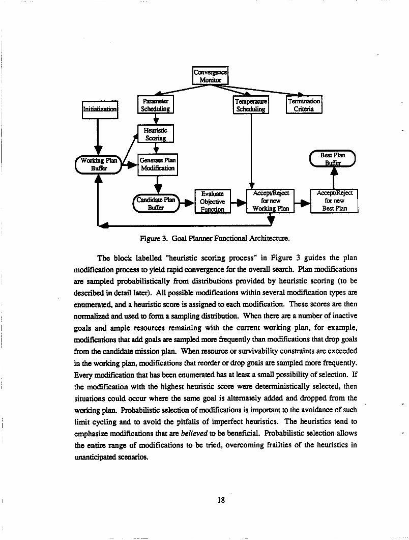
Figure 3. Goal Planner Functional Architecture.

The block labelled "heuristic scoring process" in Figure 3 guides the plan modification process to yield rapid convergence for the overall search. Plan modifications are sampled probabilistically from dismbutions provided by heuristic scoring (to be described in detail later). All possible modifications within several modification types are enumerated, and a heuristic score is assigned to each modification. These scores are then n o r m a k d ' and used to form a sampling distribution. When there m a number of inactive goals and ample resources remaining with the current working plan, for example, modifications that add goals are sampled more frequently than modifications that drop goals from the candidate mission plan. When resource or survivability constraints are exceeded in the working plan, modifications that reorder or drop goals are sampled more frequently. Every modification that has been enumerated has at least a small possibility of selection. If the modification with the highest heuristic score were deteministically selected, then situations could occur where the same goal is alternately added and dropped from the working plan. Probabilistic selection of modifications is impurtant to the avoidance of such limit cycling and to avoid the pitfalls of imperfect heuristics. The heuristics tend to emphasize modifications that are believed to be beneficial. Probabilistic selection allows the entire range of modifications to be tried, overcoming frailties of the heuristics in unanticipated scenarios.

18

The parameter scheduling box in Figure 3 adapts the skewness of the heuristic scaring sampling distributions as a function of the convergence of the search process. Early in the process, when the best plan utility is far from the utility upper bound and the resource use and survivability for the working plan arc far from constraint boundaries, the parameters are scheduled to sample more uniformly from the range of possible modifications. At this stage, the search is venturesome. At later stages, the scope of the search is n m w e d and the sampling emphasizes only those modifications that have high heuristic scores. The time available for planning can also be used in scheduling. At all stages, the ratio of incremental value added to incremental cost incurred is the basis for a powerful heuristic.

Tempcram scheduling for simulated annealing may be performed according to a number of different prescriptions. For example, the temperature may be scheduled as a monotonically decnasing function of time, or it may be scheduled adaptively as a function of the working plan utility and the utility upper bound. If a reliable upper bound can be determined, the adaptive scheduling can yield improvement in convergence rate at the expense of occasionally freezing into a near+ptimal solution. Research is currently under way on systematic approaches to optimal temperature scheduling.

The tQmination criteria include timeout for the m h process and several variations on a diminishing r e m s test. The latter compares the best plan utilities at successive time intervals.

In planning applications involving a variety of constraint fonnulations, it has been observed that the plan modification heuristics are of first order importance in achieving rapid convergence to near-optimal solutions. With good heuristics, acceptable results are obtained at high temperatures (i.e., accepting all modifications) as well as along an annealing schedule. Hence, the use of good heuristics decreases the sensitivity of the search process to the annealing schedule. However, the simulated annealing architecture dots Seem to provide a greater degree of robustness to the search process. For the stochastic mvelling salesman problem [4] involving ten frez goals, the heuristically-guided goal planner with simulated annealing yields the optimal solution in all cases studied in an average time of 2.5 seconds on a 68000-based microcomputer.

19

. . 2.3 iecuve Funcnon E V-

The formalism for the o b j d v e function ("utility") evaluation has been discussed in Section 1.3.1. At this point, we elaborate further on computational details. The process for evaluating the utility is illustrated in Figure 4. Three methods are discussed. (1) direct enumeration, (2) Monte Carlo and (3) Gaussian Approximation.

Event Tree MOdClS b Branch R(Gi I MP)

~ Probs.

utility Evaluation

Figure 4. Steps In The Utility Evaluation Process For A Mission Plan (MP)

Proceeding from right to left, the last box is the trivial evaluation of Equation (1). The evaluation of the Pr (Gi IMP), as discussed in Section 1.3.1, depends on the expansion of the event trce illustrated in Figure 2, yielding values of the planning state variables (i.e., arrival time, cumulative resource use, survivability) and probabilities comsponding to each possible manner of arrival at location Gi. The probabilities associated with the individual nodes in the event me am evaluated as the product of conditional (branch) probabilities that describe the likelihood of outcomes comsponding to particular events given the entry conditions at the beginning of each leg. The conditional (branch) probabilities, in turn, are evaluated for the assumed event types for each mission leg by the use of models (i.e., resource use, survivability) applied to the onboard database and using the waypoint paths that have been generated by the (far-term) waypoint planner. The onboard database includes a griddcd map indicating elevations, threats (or probabilitiy densities for threats), and winds in the environmental portion of the database and goal locations, values, etc., in the mission plan portion of the database.

The utility evaluation process is initialized with the currcnt values of the time, resources (Le. fuel and ardinance), estimated location, and the particular mission plan (MP) to be evaluated. The mission plan may be the current plan or any candidate alternative plan. For the samc waypoint paths and onboard database, a given MP will exhibit different utility values depending on the initial conditions. For example, different values of the absolute

20

,

time or fuel remaining at a given cunrcnt vehicle location will result in diffennt R (Gi IMP) and diffennt utility values.

The r~source use and survivability models use the specified initial conditions and onboard database to calculate predicted arrival time, resource use, and survivability for each of the possible sequences of events that can occur on the way to each goal location. The model cdcu€iuions cannot bepe@onnedprejlight and used as stored data because both the initial conditions and onboard database may change during the execution of a mission. That is, at a given time, the vehicle location and resource usc may differ from that predicted by the prefight mission plan and the database may be modified as a result of fusion of information €tom onboard sensors and/or received communications. In addition, the number of possible mission plans is combinatorially large. For all of these reasons, the probabilities associated with the nodes of the event m e must be calculated in-flight and cannot be precomputed and stored in the onboard database.

The following example will help illustrate the process of enumerating nodes of the event tree. Consider that the vehicle tactical response is triggered on detection of hostile emitter activity by a radar warning receiver and the assessment that this corresponds to a valid k a t . The pilot initiates deployment of electronic warfare countermeasures (i.e., jamming), masking countermeasures (i.e., chaff, flare decoy resources) and/or evasive maneuvers. For purposes of far-term planning, the entire mission is anciticipated to consist of zcro to perhaps a half dozen of such tactical responses. (It is unlikely that low- survivability missions resulting in engagement by dozens of surface-to-air anti-aircraft assets will be planned). For each tactical response, the expected impact on resources (Le., fuel, expendable decoys) and time is specified as a function of information that is available in the mapped database such as threat type, terrain, etc. The resource and time impacts can be estimated fmm combat experience or fiom detailed engagement simulations.

The different branches in Figure 5 correspond to the possibilities for 0 through k tactical responses for each mission leg a subsequent survival. In other words, "0 responses & survival" implies that hostile forces either are absent, or that they fail to target the vehicle or that they otherwise fail to successfully engage the vehicle even though then are no vehicle maneuvers. The branch labeled "1 tactical response and survival" corresponds to the case when the vehicle perfoms one response resulting from either a m e or a false alarm, and that hostile forces are either absent or otherwise fail to target or successfully engage the vehicle.

21

0

0 tactical responses and survival 1 tactical response and survival 2tacticalresponses and survival

k tactical responses and survival

Figure 5. Enumeration of Event Tree Possibilities

The threat models used to predict the probabilities for each branch reflect the probability of detection given the intcrvisibility and the hostile radar performance parameters (i.e., range, clutter rejection, probability of being functional and turned on, etc.), the probability of successful engagement by hostile forces given no vehicle countermeasures or maneuvers and the weapon effectiveness in the presence of tactical responses. The arcal density or areal probability density of threat systems along the path, the vehicle exposure time in the vicinity of these h a t s , and vehicle flight parameters such as flight mode and altitude arc additional factors in the models used to prcdict the branch probabilities. In the context of far-term planning, given the uncertainty in knowledge of threat deployments and capabilities, the emphasis in modeling is placed on the capture of c o m t trending and fast extcution rather than on (argueable) high fidelity.

Hence, each of the nodes at any goal location represents a particular sequence of possible events along the legs of the mission plan leading to that goal location. Each node has an associated arrival time, resource use and survivability estimate. The sum of the probabilities of all (survival) nodes at any goal location gives the net vehicle survivability given the initial conditions, mission plan and underlying database and models. The sum of the subset of nodcs whose arrival time, resource use and vehicle capability estimates simultaneously satisfy a l l mission plan constraint specifications (unique to each mission) is identitied as the probability of successfully completing that goal, Pr (Gi I MP).

Far a simplified system involving only uniform branch probabilities and the simplest of modcls ("stochastic travelling salesman problem" [4]), the computation time to

22

evaluate the objective function by direct enurnration, by Monte Carlo techniques and by a Gaussian approximation is plotted in Figure 6.

1000

a 800

t I 600

W

e

s 5 400

i= 200 E

0

f MXPIWCPUTI~~ > I 2 4 6 8 10 12

# Goals

~ ~~

Figurt 6. Computation T i For Different Methods For Objective Function Evaluation.

This figure clearly illustrates the exponential (in the number of goals) growth of computation time of the dircct enumeration procedure just described. In generating the data for Figure 6, there wcn only wo branches per mission leg (Le., the portion of the mission between two goals). When there are sevcral event branches per leg and less trivial models to be evaluated for the branch probabilities, direct enumeration becomes computationally intractible except for missions with only a few goals.

The Monte Carlo evaluation involves the estimation of the Pr (Gi I MP) by repeated mission simulations via branch sampling. The R(Gi IMP) are all initialized to zero. Each trial then consists of a simulation of one particular sequence of events for a mission plan, starting with the currcnt location, time, and nsource level and predicting forward to the end of the mission. The selection of the branch to be followed for each mission leg is performed by sampling from a probability distribution (formed from the branch probabilities) using (pseudo) random numbers. As each leg is sampled, the cumulative

23

time and resource use and node probability value is generated for that trial. The estimate for each Pr (Gi I MP) is incrcmented by the sampled nodc probability if the corresponding time and resource use satisfy the problem constraints. When the last leg has been sampled, the process is repeated. After a fixed number of trials have been completed, the Pr (Gi IMP) estimates arc normalized by the number of trials to yield the final results. Alternatively, the second moment of the Pr (Gi I MP) can be estimated at the same time as the mean value, and the standard deviation in the estimate used to control the number of trials taken according to some sptcificd level of estimation accuracy. This is not generally done except for test purposes because of the additional multiplication and addition steps that arercquircd

The Monte Carlo estimation process can be viewed as a "mini-simulation" of the IMllitindQ of the mission according to the mission plan. The uncertainties of plan execution are modeled as stochastic selections between branches corresponding to different events on each mission leg. In the Monte Carlo pmess, however, the probability distribution used to select between branches can be altered for purposes of improving numerical efficiency, provided that the estimator is modified to result in an unbiased estimate [7]. For example, a strict ("analog") simulation would enumerate the non-survival nodes. When those nodes wen sampled during the Monte Carlo estimation process, that trial would terminate when a

nonsurvival node was sampled, resulting in no conmbution to the Pr (Gi I MP) of the goals downsaeam of that nonsurvival node. This results in a deterioration of accuracy (i.e., larger ratio of standard deviation of sample mean to sample mean for the Pr (Gi I MP) ) for goals later in the mission plan relative to the goals close to the c m n t vehicle location. To achieve a stated level of statistical accuracy for all goals then requires a larger number of trials, with computational cost scaling linearly with the number of trials.

Another possibility is to sample uniformly for which branch to choose for each mission leg and to weight the contribution to the estimate of Pr (Gi IMP) by the actual branch probability, multiplied for each successive leg. This also is an unbiased estimate, but with even worn statistical Mor characteristics! The best estimator appears to be obtained by sampling according to the normalized ratio of the survival branch probabilities (i.e. p&, where pi = probability of node i and the summation extends over all nodes for a given location). The branches that contribute most to the solution are sampled more frequently (Le., "importance-sampled"), and the use of the survival branches only (node probabilities conditioned on survival) is akin to the use of the "expected value estimator" from the theory of Monte Carlo estimation [8]. For far-field planning applications

24

involving 20 goals, the importance -sampled process with expected value estimator has been observed to yield satisfactory statistical accuracy (Le., -5% relative deviation, where relative deviation is defined to be the standard deviation divided by the sample mean) for the Pr (Gi IMP) with as few as 25 trials. When new "best plans" arc found and for other critical decisions in the optimization proccss, the number of aials can be increased to 100 or 400 for greater accuracy. The relative deviation scales inversely as the square root of the number of trials, with 100 trials showing a factor of two improvement and 400 trials a factor of four improvement over the 25 trial estimate.

We see in Figure 6 the results for the case of 25 trials for the stochastic travelling salesman problem with only two branches and uniform branch probabilities. When there arc more than two brances, the Monte Carlo time is almost unaffected whereas the direct enumeration computational time increases substantially. If there were four branches for each mission leg, for example, the Monte Carlo would be less expensive than the direct enumeration when then wen only four goals remaining in the mission plan. The Monte Carlo process permits tractable estimation for event tfccs of arbitrary length and structure. The Gaussian approximation, however, is seen to be substantially cheaper than both Monte Carlo and direct enumeration. The linear growth with number of goals for both Monte Carlo and Gaussian approximations arises from the operations involved in prediction of time and resource usc for each mission leg in the remainder of the mission. The timing results for the Gaussian approximation arc reproduced on an expanded scale in Figure 7. The time-axis intempt of about 5 msec arises from the evaluation of an approximation to the error function that is used in the Gaussian approximation.

The Gaussian approximation consists of accumulating the mean and standard deviation of the time and resources used to each goal of the mission plan and then using the statistics of the Gaussian distribution to evaluate the probability that the timc and resources simultaneously satisfy the specified problem constraints. When the number of nodes in Figure 5 is quite dense, it is to be expected that the discrete probability density (=presented by the node probabilities) may be reasonably approximated by a continuous distribution such as a multivariate Gaussian disrribution. The Monte Carlo estimation process must nonetheless be used to filter out the effects of the Type I and Type 11 errors discussed in section 2.1.

25

4 I 0 2 4 6 8 10 12

# Goals

Figurc 7. Macplus Execution Time For The Gaussian Approximation For The Utility

2.4

The function to be optimized (maximized) in the application of simulated annealing to planning is the mission plan utiZity. The optimization proceeds by selecting and sequencing a subset of goals and the multiple path choices between goals. In practice, several hundred candidate plans out of the N! possible plans are generated and compared on the basis of their expected utility. The candidate plans arc interrelated in that they are constructed incrementally, or in other words, each successive candidate plan is a modification of the preceeding plan. The modifications involve adding, deleting, reordering, swapping between active and inactive goals, and reversal of segments of the mission plan according to a random sampling from a set of possible modifications. At every step in the sequence of candidate plan generation, a modification that is vastly deleterious to the utility value is rejected and a different modification is attempted. The utility value can decrcase as a result of deleting high value goals or constraint violations (time or resource). At every step, a modification that is slightly deleterious to the utility

26

value is accepted probabilistically, with higher probability if the loss in utility (with respect to the previous candidate plan) is small and the "temperature" is high. The temperature is initially set to %igh'* values that permit almost all modifications to be accepted and gradually lowered as the process converges. At the end of the process, at low tempcraaucs, only modifications with improved utility are accepted. At high temperatures, the process considcrs modifications across the range of the configuration space enabling the c o a m structure of the mission plan to be determined. At low temperatures, the process resolves the finer details of the mission plan allowing only minor substitutions and transpositions of goals [9].

Given the definition of the mission plan, the search space and the objective function, the crux of the simulated annealing optimization process is the generation of the candidate plans and the scheduling of the tempcram parameter. Candidate plan generation is completely specified by the selection of the initial candidate plan and the recursive algorithm for generating modiflaions at each step of the process. The initial plan can be set to the trivial plan of "go directly home" from the current vehicle location. In this case, the annealing proccss will add goals and build up a plan that maximizes the value of goals expected to be successfully completed while satisfying all constraints, including global resource and survivability constraints. Alternatively, the initial plan can be set to the mission plan that is currently being executed (but is perhaps no longer viable). Although. the globally optimal plan will be produced asymptotically, regardless of initialization, the outcome in h i t e time (Le., af'tcr only a few hundred candidate plans) will tend to preserve morc of the features of the c m n t plan if the current plan is used for initialization. There an typically a number of plans of approximately the samc utility in the neighborhood of the optimal solution. Although thm may not be much difference between the utility of plans

derived from diffennt initial conditions, it may be *able to present the pilot with a plan that shows some relation to the cumnt plan.

The most important contributor to good performance is the p l a modification algorithm. The components of this algorithm are termed heuristics and are described mort fully in the next section. We have found a number of heuristics that appear to be robust across a spectrum of problem specifications. Nonetheless, then is always some domain dependence to heuristics.

For travelling salesman optimization problems where random plan ("tour") modifications are employed, the scheduling of the annealing temperature can significantly a f k t the performance (Le., the speed of convergence and ultimate de- of optimality) of

27

the annealing process. When powerful heuristics arc employed in order to ensure rapid convergence to near-optimal plans, the temperature scheduling becomes less important. It is st i l l recommended to start the process at a relatively high temperature and terminate at a low temperature as such scheduling will enhance the robustness of the optimization process. The fact that good solutions will (usually) be obtained regardless of the temperature schedule is due, in part, to the scheduling of heuristics with the degree of convergence of candidate plans to known upper bounds on plan utility. Hence, venturcsome plan modifications arc propostd early in the annealing process and "finishing" or "polishing" modifcations arc sampled preferentially when a working plan with a high utility value has been selected.

Regarding the annealing temperature schedule, Figure 8 shows a number of schemes that have been proposed in the literature [ 10,11,12]. All curves have been normalized to a starting temperature of 2 utility units. In other words, the initial temperature is twice the maximum (upper bound) utility. The curve identified as "l/h(l+t)" represents the fastest rate of cooling that can be theoretically demonstrated to yield a globally optimal solution. Each time point represents an "equilibrium" point in that the fluctuations in the objective function value averaged over a number of mWications at that temperature arc allowed to "settle" to approximately steady levels. The time interval spent equilibrating at each temperature point is sometimes called an "epoch." There are

theoretical prescriptions for the tumination criteria, in other words, the lowest temperature, but a value of -0.2 utility units may be taken as a practical approximation to zero temperature. Hence, to anneal from T=2.0 to T4.2 with the "l/ln(l+t)" theoretical schedule requires on the order of 10,OOO epochs. Since the temperature is changing so slowly between epochs, the epoch-size can be unity (Le., one modification) after the frrst several epochs. Nonetheless, this process has been found to be far too slow for practical application.

28

2.0

L Q) 1.5 a E c1

a E laO

0.5

0.0 0 10 20 30 40

Time t

Figure 8. Roposed Annealing Tempcram Schedules

The curve labeled 'Tl+l = .95*Ti" nprcscnts a morc practical prescription. It can be seen to decrease morc slowly than the theoretical schedule until the intersection at the 21st epoch. The factor of ten temperature drop is achieved after approximately 45 epochs, but the cpoch-size may need to be 8 to 64 modifications for a total of perhaps one to several thousand modifications. The same functional fonn can be used but with other multipliers, as in the Ti+1 =L .9O*Ti" and Ti+1= .,Tit' curves. In these cases, the epoch-size needs to be slightly larger than for the 'Ti+1= .95Tf case, but the total number of modifications can be substantially less. The use of these morc rapid cooling schedules frequently results in convergence to suboptimal solutions. There is a tradeoff between the degree of optimality (or the probability that an optimal solution will be obtained) and the time allowed for cooling. Since the (time or ensemble averaged) objective function value is known to exhibit an "S-shaped" variation with annealing temperature (reminiscent of the internal energy as a function of temperature for a fmt-order phase transition), it has been recommended [lo] that the temperature can be cooled rapidly (i.e.,Ti+l = .8*Ti ) on the initial high temperature, flat portion of the S-curve, switched to a slow cooling (Le., Ti+l=

.95*Ti ) for the rapidlychanging (phasc-transition) region, and switched back again to rapid cooling for the low-tempcram flat-portion of the curve. The "l/(l+t)" curve

29

represents an even more radical departure wherein rapid.cooling is used along with a

replacement of the Boltzmann e 'm factor with the Cauchy-Lorentian factor: AU

and with the use of the Cauchy-Lorcntzian distribution to generate (kV [(kV2 + (m21

modifications [12]. This has been labeled "Fast Simulated Annealing" and has shown impressive results in comparison with random modifications (i.e., no heuristics) and the theorctical schedule.

For planning applications, we have devised an adaptive temperature schedule that uses information on the known upper bound of the mission plan utility and that incorporates intuitively correct trends. Defining the dimensionless quantities a, p as:

a = &, O S a S 1 (3)

-AU B = O ! q S 1

when U, = Utility value of current working plan Urnax = Utility upper bound

AU = Decrease in utility of candidate plan with respect to UC

The probability of accepting downhill modifications is:

aP f(a,P) = e - (4)

Note that the temperature is in units of Urnax. For an adaptive schedule, we desire the following trends for f ( sP) :

We also desire that the rate of approach to these limits should be a-dependent and steeper as a + 1. One example of a functional form that exhibits the desired trends (at least for Equation 6) is:

30

This is labeled the "NH" recipe and is plotted parametrically in Figure 9. The likelihood of accepting downhill modifications decreases as the utility of the current working plan approaches the utility upper bound and as the size of the downhill jump increases.

1 .o

t. 0.8 .I - .I 3

8

0.6 LL

s 0.4 8

2 0.2

c.

0.0 0.0 0.2 0.4 0.6 0.8 1 .o

Beta

Figure 9. YV"' Recipe Adaptive Temperatun Schedule

Another functional form that exhibits the corrcct wends is:

as --

- * -

This is labelled the "OLD" recipe and is plotted in Figure 10. This recipe represents somwhat slower cooling and allows largez downhill jumps as U, + Urn=. Either recipe gives acceptable performance in terms of the best plan utility in finite time, the relative performance depending on the problem specification and being largely masked by the overwhelming effcct of the heuristics.

31

1 .o

0.8

0.6

0.4

0.2

0.0 0.0 0.2 0.4 0.6 0.8 1 .o

Beta

Figure 10. "OLD" Recipe Adaptive Temperature Schedule

2.5 Heraistics 2.5.1 ModificationTvgs

As previously mentioned, the modifications to the working plan to generate new candidate mission plans are drawn from a set of modification types. Typical modification types include:

Inactivdactive goal swap Addition of an inactive goal Rtardcring of an active goal Segment deletion

'Twwpt" (combination segment deletion and reversal) order swap between two active goals

segmcntnvcrsal

Heuristics can be constructed with a reduced set of modification types, such as add, drop, and nordcr. The morc complex modifications must then be constructed from consecutive generation and acceptance of the simpler modification types. The incorporation of the larger set of modification types has been found to yield more robust finite-tim performance in terms of degree of optimality and fiequcncy of finding the optimal solution for problems

32

where this is known [4]. The set of modification types listed above encompasses essentially of the order N2 (or more) modifications, that is, the modifcations involving enumeration of I@ possibilities when N is the total (active+inactive) number of goals. Since the heuristics involve the enumeration and "quick scoring" of each possible modification followed by sampling for a particular modification for the generation of each candidate mission plan, the limitation to order @ (or fewer) is a practical necessity to accomodatc problem definitions involving as many as 20 or 30 goals on near-term flyable processors. Of course, heuristics could be constructed using higher-order modifications if the methodology of enumerating each possible modification were abandoned and the resulting modifications could be scored efficiently. In any case, the total computational time budget is apportioned between two major components: time spent in generating modifications and the timc spent in evaluating the objective function for each candidate mission plan. For a fixed total time budget, if more time is spent in generating good candidate mission plans (i.e., plans more likely to be accepted), then fewer candidate plans can be evaluated. At the limits of random (Le., unintelligent) plan modifications, very little time is spent in finding modifications but the quality of the resulting candidate plans is poor. At the other extreme, all of the time budget can be spent in devising a single candidate plan. The quality of the final solution is apt to be poor at both extremes of apportioning time between plan modification and plan evaluation.

Illustrative examples of the Merent modification types are depicted in Figures 1 1 - 17. A portion of a mission plan with five active goals (filled dots) labelled A,B,E,F, and G and three inactive goals (unfilled dots C,D, and J) is shown along with the directed links between goals. This is highly schematic in that a waypoint path between goals is represented as a single vector. In Figure 11, the inactive goal D is swaped for the active goal B. In other words, B becomes inactive and D becomes active. The sequence location of D in the plan is coincidentally but not necessarily the same as that for the goal it is replacing. In general, that are ordcr N possibilities for goal substitutions and order N possibilities for the sequence location of the substituted goal for a total of order N3 possibilities for this type of modification

33

Figure 11. Inactivdactive Goal Swap Modification Type.

Figure 12 shows a goal addition type modification. Formerly inactive goal D is added in the sequence between goals E and E Here again, there arc order fl possibilities for this type of modification. This is true for a l l of the remaining types as well. Figure 13 shows a reordering type modification wherein the sequence order of (active) goal F is changed so that goal F is executed immediately after goal A, the sequence order of the

remaining goals being unchanged.

I

Figm 12.Addition Of An Inactive Goal Modification Type.

OC

.

Figure 13. Reordering Of An Active Goal Modification Type.

34

Figure 14 is an example of a segment deletion modification type. The mission plan segment between goals A and F is deleted, including goals B and E, and the goals at the endpoints of the deleted segment have their links connected There are order N possibilities for the beginning of the segment to be deleted times order N possibilities for the length of the segment. The segment reversal modification illustrated in Figure 15 shows a change in dircction for the segment between goals B and F, with the links to the segment endpoints appropriately connected. The "two-opt" type modification in Figure 16 is a hybrid modification that can be thought of as a segment reversal (B-E-F) followed by a segment deletion resulting in the dropping of goal E from the active goal list. Figure 17 shows an example of a (sequence) order swap between (active) goals A and F. That is, after the modification, goal F becomes the beginning of this portion of the mission plan and goal A follows goal E (Le., the old sequence position of goal F). Although hybrid modifications can be constructed from simpler modification types, the likelihood of acceptance of successive candidate plans embodying the simpler modifications may render these constructions unlikely when only several hundred modifications axe generated.

I

A 0 D

B O O E

"C

0 J

~~~

Figure 14. Segment Deletion Modification Type.

A LDo mr; A F Y G

8 E B -E OC OC

Figure 15. Segment Reversal Modification Typt.

35

c,

Figure 16. Two-opt Modification Type.

A \Do mco B E B '.E

OC OC

Figure 17. Order Swap Between Two Active Goals Modification Type.

The modifications are implemented in software by reassigning sequence pointers (forward and backward-linked) and reassigning logical variables used as goal "activity flags." The time, resources used, and survivability cost for the transit along the waypoint path between euch goal and every other goal is stortd in a square matrix (revemability is not assumed). Hence, the impact on time, rcsouces, and survivability for each modification can be evaluated by table lookup and a few additions or subtractions. For example, for the inactive goal addition example of Figure 12, the impact on fuel used is:

Ahel = fuel(E,D) + fuel@,F) - fuel(E,F) (10)

where fuel(E,D) = fuel required to transit path between E and D

In this manner, time, resource, and survivability impacts for all modifications can be quickly assessed and the global resource use and survivability evaluated recursively with only a couple of addition operations instead of beginning the summation over the entire mission plan anew. The time, resource, and survivability impacts of each modification are

36

used to form probability densities that are used to sample for a particular modification to fonn the new candidate mission plan. These probability densities need only be regenerated upon acceptance of a new candidate mission plan as the current working plan. Upon rejection, for example, a new modification is sampled from the same distributions with a "new" (pseudo-) random number.

. . 2.5.2 -sac S t r u c m

The heuristic structure for the goal planner has been derived from a few underlying concepts and from much experimentation. The underlying concepts are (1) the use of the incremental value to cost ratio heuristic, (2) the detection of global constraint violations to govern alternation between plan construction and plan reorganization strategies, (3) the use of an approximate utility heuristic to compare modifications and (4) the use of a multi-start strategy.

In the present incarnation of goal planner software and design, there are three heuristic sampling algorithms embodied in thrce subroutines and labelled as "stages" A,B, and C (note: no relation to the goal labels in the examples above). In stage A, only goal additions and increasing value swaps between active and inactive goal sets are considered. Recall that each goal has an associated value assigned during the initial problem specification by human planners. M m impartant goals are assigned higher values than are goals of lesser importance. In stage A, only those swaps between an inactive goal of higher value than an active goal are considered along with straight goal additions. The probability density that is used for sampling one modification out of the entire set of possible stage A modifications is constructed using a value-to-cost heuristic. That is, a sampling distribution is formed:

Where mi = incremental vdue to cost ratio for the i* modification pro = I lomahd . sampling density for all M modifications

37

In stage A, modifications arc sampled successively h m this heuristic for a fixed number of successive modifications or until there are no more modifications that show an increasing value. To avoid the numerical effort of the normalization process in Equation 12, the distribution of values for the numerator in Equation 12 (the "heuristic scores") are sampled by binning into 50 equal intervals between the minimum and maximum scores and sampling from the populated bins with the highest heuristic scores. Once a bin is selected, the particular modification whose score falls within that bin is sampled uniformly from among all modifications falling within that bin. The selection of the particular functional form for the heuristic score, the use of 50 bins, and the prescription for sampling the topmost bins represent engineering choices. It is difficult to establish optimality of all of these choices by virtue of the size of the parameter space and the statistical difficulties in conelating the choices with performance measures.

In stage 8, the goal reorder, segment reversal, and equal-valued goal swap modifcation types are considered. In all of these modifications, the sum of goal values (irrtspcctive of the R(Gi I MP) which are unknown prior to evaluation) remains invariant as a result of the modification. The purpose of stage B is to rationalize the working plan by rearranging links or goal swapping to minimize resource use, maximize survivability, or otherwise contribute to higher R(Gi I MP) values. Stage A assembles a set of goals in approximately the right sequence and stage B attempts to minimize resource use and allow more goals to be added in a subsequent cycle ofstage A. The sampling distribution is fomwd as:

j-1

where

Afuelj = incremental fuel for the j* modification

The use of the second power of the fuel saving biases the distribution to favor fuel saving modifications and is a simple evaluation relative to the range of functional forms that could be used. If a modification results in extra fuel expenditure, then it is excluded h m the set of M' mDdifications of the indicated types. If any modification results in violation of global constraints on time, resources or survivability, it too is excluded from consideration in either stageA or stage B. The binwise sampling technique is applied in stage B as it is in all

38

stages. Stage B is continued until either a k e d number of successive modifications have been sampled or thcrc arc no xmdifications that result in fuel savings.

In stages A and B, modifications wen excludcd from consideration if the expected value of time, resources or survivability violated global constraints. In stage C, all modification types are considered using a quick Gaussian approximation for scoring the modifications as described blow. Given a -me constraint Rc and a finimum r e q u w proba-- we require: .. . .

rN@ , z ) d E 2 kr (14) 90

whcrc

it = mManresourceuse - cr = true standaxd deviation of resource use N = assumed Gaussian distribution of resource use

A A

Since the true mean and standard deviation must be estimated, resulting in Rand a, respectively, the constraint expressed in Equation 14 is postulated to be equivalent to the

A

q-tthatas G O , when: A

Rc - R erEl(2kr - 1) 00 =

Since is a problem specification, the expensive inverse error function in the denominator

of Equation (15) need only be evaluated once during initialization. The values of aand a, for each modification in stage C are then used in apenultyjiutction that multiplies the sum of the goal values for all active goals in the mission plan. The penalty function takes on values near unity when cr S .90*a,, it takes on a small but non-zero value when

cr2 l.lO*cro. and it varies linearly in between these limits. The heuristic scoring in stage C thus factors in the uncertainty caused by the different possibilities of the event tree and the effects of the global constraints in an approximate but quickly executing manner. Hence, all modification typcs may be scored on the same basis, without arbitrary weighting factm to cxpxess the relative importance of resources versus survivability, etc. Otherwise, goal addition modifications which generally use more nsources andpotentially add value (but may actually lower the utility because of constraint violation) cannot be compared with goal reorder modifications that do not change the sum of goal values but may well change

A

n

A

39

the Pr(GilMP) and hence the actual utility. Stage C is repeated until either a fixed number of modifications have been sampled or there are no favorable modifications to be sampled.

A

Initialize Trial Plan

# Tries or Stage A

Heuristics No Good I

0

\r Moves

Stage C Heuristics

r

I t #Tries

Moves

Stage B or Heuristics No Good

Exit

Figure 18. Tnal Plan Generation Heuristic Structure

If there are better plans that result after the stage B and C modifications relative to the best plan at the outcome of stage A, then stage A is entered once again with initialization from the outcome of stage C (total time permitting). This is done because the plan rationalization that has o c c d in stages B and C may now permit more goals to be added within the global constraints. If then was no detected improvement between stages A and

40

C then a new working mission plan is initialized and the process is repeated until timeout. The trial plan generation heuristic structure is illustrated in Figure 18. The beszplan that has been found is available at all times. Because of the sampling involved in the generation as well as acceptance of modifications, the trajectory of working plans is apt to be different even if the same initialization is used on subsequent cycles through stages A through C. The reinitialization is tantamount to the selection of "non-local" modifications, that is, modifications that an radically different from the currcnt working plan. For finite- time in which extremely fast convergence to optimal or near-optimal solutions is desired, this feature of the heuristic structure seems to be quite impartant.

2.6 To Other P b i n e Elements

Apart from the specification of goals and associated values and constraints (i.e., time, ordering, survivability), the goal plannerrequires an array of cost, resource and transit time between evay pair of goals (in both directions) for a multiplicity of paths between each pair reflecting different points on the cost-resource operating curve. With this infomation and on-board infomation on location, time and resource supply, the goal planner can project lethality cost, resource and timc use along any pposed mission plan by simple addition over a l l intergoal links in that plan. This interface information is summarized in Table 1.

Note that the environmental database information (Le., terrain, winds, threat locations, exclusion zones) is not used directly by the goal planner, nor is the detailed path information from the waypoint planner. With regard to the latter, only the time, fuel,

expendables and lethality cost numbers an used by the heuristics. The utility evaluator uses these numbers along with the additional infomation of branch probabilities and (models of) fuel, time, resource and lethality consequences for each of the branches. Hence, relatively few numbers arc input to the goal planner and these arc updated slowly if at all (i.e., low bandwidth inputs).

41

Item

Mission Specifications

Cumnt Vehicle Status (pndiction initial data)

Waypoint Path Data

Description ~~

Goal locations, values, time constraints, ordering constraints, goal status (i.e., already executed), position tolerance, goal actions (and associated time, lethality cost, resource use)

Estimated location, estimated navigation error, fuel supply, ordinancc/expcndables (chaff, decoys) supply, quipmcnt operability (propulsion, ESM, offensive avionics, navigation, communication), time

Lethality cost, fuel use, expendables usage, transit time for a multiplicity of resomx constrained optimal paths (Le., -5 paths per pair) Also, event tree branch probabilities or mtrics from which branch probabilities can be estimated for each intergoal path

Table 1. Interface I n f o d o n Inputs To The Goal Planner

The fuel, time, resource and lethality cost for each waypoint path, along with the event me branch information, is generated by the waypoint planner. The waypoint planner uses the terrain, winds, h a t , and exclusion area information in the environmental database, along with predictive models for lethality cost and resource usage, to determine the waypoint paths and the summary information that is required by the goal planner. To reduce the computational time requirements for the on-board system, the information in the environmental database is processed preflight into a database for waypoint planning. The processing is done in a way that allows the waypoint planner to estimate fuel, time, resource and lethality cost by summing prestored internodal quantities. In addition, a multiplicity of waypoint paths between all known goals is generated preflight. As the onboard database is updated with new sensor information or communications, only the nodes and paths thus affected need be recalculated in-flight.

In the present concept, none of the far-field planning components interface to high bandwidth or imaging sensor data or communications directly. All of this information is merged into the databases that support far-field planning. The near-field or trajectory planning levels deal with the high bandwidth information in rendering tactical decisions in concert with the mission management executive and its associated situation assessment function.

42

Finally, the output from the goal planner is the ordered sequence of goals that achieve the highest objective value within the problem constraints (including calculation time) and the coarse-level waypoint path selectcd for each intergoal segment. The arrival time/spd schedule is calculated by the t imehe management function called internally by the goal planner. The coarse-level waypoint path is used by lower levels of planning/control. The goal planner may also be configured to provide information to the waypoint planner on the subset of intergoal links that need to have waypoint path parameters calculated. This selective thinning of the array of intergoal links may be used to help cut down the total calculation time required by the waypoint planning process that supports the goal planner.

43

SECXION 3

WAYPOINTPLANNING

The waypoint planning problem is a shortest-path problem over a network of nodes. In the context of waypoint path planning, the term nodes is used to indicate the set of possible spatial locations through which the planned vehicle trajectory must pass. The nodal network concept maps the path-search process onto a discrete, finite dimensional space. The problem may be described as that of fmding a path that minimizes the path cost, Zc(i,j), over all possible paths from node point S to node point G, subject to some form of constraint on the expended nsources, wid). Here, c(i,j) and r(ij), respectively, represent the path cost andresowccs expended in &tion from node i to node j, and the summation extends over all transitions along each path starting at node S and ending at node G.

Procedures for finding the mincost path are generally recursive in nature, with the recursive step involving the growth of a "tree" of path branches to "successor" nodes from a suitably chosen "parent" node. In case of more than one path-branch to a node, branch pruning logic is employed to select the branch on the min-cost path. The tree generation process terminates when the goal node has been reached and upon satisfaction of exit

criteria.

3.2 Overview

An efficient implementation of the above process can be carried out using the A* algorithm, involving a bookkeeping arrangement of two types of stacks, namely "open" and "closed", for the nodes on the tree [ 131. Associated with each node is the cost of the path from the start node, and a pointer that indicates the parent (predecessor) node. The search starts by placing the start node on the open stack. The recursive step of tree growing involves the selection of a node for expansion and the generation of its successor

45

PREZEDING PAGE BLANK NCY" FILMED

nodes. The node n with the minimum of value of the "expansion function", f(n), among all nodes on the open stack is selected for expansion. The expansion function for the successor nodes, n', is given by Equation 16

f(n') = f(n) + b(n,n')

f(S) = 0 (Start node initial condition) (16)

Thus, the expansion function is additive and its nature is determined by the function b(n,n'), of which there arc several logical choices. For a "uniform cost expansion," the function b(n,n') is the path cost function c(n,n'); for a "uniform resources expansion," b(n,n') is the resource use function r(n,n'); for a "breadth-first" expansion, b(n,n') = 1. Upon expansion, node n is placed on the closed stack. As regards its successors, every successor n' of n is placed on the open stack and the cumulative path cost function is incremented:

C(n') = C(n) + c(n,n')

C(S) = o If any n' was already on either stack prior to expansion of n, then the lower of the

two C(n') is selected and the parent node pointer is set to reflect the chosen branch. If n' had previously been on the closed stack and its newly expanded cost is lower than its previous cost, then n' is switched to the open stack.

The search is terminated when the node chosen for expansion is the goal node, or in other words, when n' = G and f(G) is the minimum for all nodes on the open stack. The mintost path is then obtained by tracing the parent node pointers back to the staxt node.

For the uniformcost expansion, the expansion function can be modified to include a heuristic function h as follows [13]:

f(n') = g(n') + h(n')

The heuristic function h(n') represents an estimate of the minimum cost to go from n' to the goal node. It has a strong influence on the computational time for the search and on the optimality of the path that results. Optimality is guaranteed if h(n') is bounded from above by the me optimal path cost from n' to the goal node. Larger values of h(n') are termed "inadmissible heuristics," and result in faster searches with potentially suboptimal

46

results. For heuristics, we have investigated the use of measures of the distance between n' and G, and (embedded) A* solutions obtained firom a backward search (Le., from G to S) on a coarser nodalhation. If optimal solutions are desired, we have not found any

general prescription that leads to a faster search than h(n') = d(n')-minimum ( c(i,j) 1,

where d(n') represents the minimum number of moves from n' to the goal node. The A* search with h(n') = 0 corresponds to Djikstra's uniform-cost algorithm [ 131. Among the search processes without heuristics, Djikstra's algorithm is the most efficient, with no node chosen more than once for expansion and, in general, no more than one path expanded to the goal.

1J

. . 3.2.1 PIPD) T-

For searches other than the uniform cost expansion, many more nodes are expanded than for Djikstra's algorithm and more than one path is expanded to the goal before the optimal path is reached. The latter feature can be exploited to yield the entire curve of resource used versus cost for all resource-constrained optimal paths. We have labeled this modified A* search process as the "Eath Independent Eerformance &termination" (PIPD) technique. A separate open stack is maintained for each resource level attainable during the expansion. Considerable simplicity obtains when the operating curve rather than the associated optimal paths is desircd The bookkeeping of parent node pointers is dispensed with and open stacks arc maintained only over a finite resource window.

For a given cost map and start and goal nodes, the PIPD technique yields a set of (cost,rcsourcc) points associated with various resourceconstrained optimal paths. This is precisely the information that is most useful to the goal planner. Once the goal planner has chosen an Operating point from this set, the corresponding (optimal for the specified constraints on rtsources) path is nconstructed by executing an A* search using a Lagrange multiplier modification to the function:

g(n') = g(n) + c(n,n') + X r(n,n') (19) The value for A is obtained as the slope of the cost-resource curve at the point selected on the curve, and is calculated in the PIPD pnxxss. The path determination is insensitive to small CTLWS in I., with a path remaining unchanged as X is varied inbetween discrete values of the Operating c w e slope corresponding to the discrete PIPD solutions.

47

3.2.2 pesulg

Some results for the waypoint search algorithm are shown in Figures 19 and 20. The example presented in Figure 19 contains a 20 by 30 network of nodes with cost function synthesized by correlated random sampling. The number or dot printed in the position for each node reprtsents the cost for traversing that node. A dot is the lowest cost, with numbers 0,2,4, ..., 8 representing increasing cost values. The map shows many low cost channels, presenting the waypoint planner with a "soft maze," one of the more challenging types of problems. A mazc with hard boundaries would permit earlier pruning of the search tree. The start and goal nodes are labeled, and two paths are shown: the broader line indicates the unconstrained resource minimum cost path; the lighter line indicates an optimal cost path corresponding to a specific resource constraint. In this example, the resource use is modeled as being Proportional to distance, with one horizontal or vertical segment equal to 10 units and a diagonal segment equal to 14 units. The unconstrained mincost path has cost value = 3.523, with resource expended = 375. The resource-constrained optimal path has cost = 3.747, with constrained resource use S 269. The goal planner might opt to use the lower resource but higher cost path if the resource saved (1) enabled additional goals to be added, or (2) permitted lower cost (and higher resource use) paths to be used to advantage elsewen in the plan.

48

Column Number ~ 1 2 3 4 5 6 7 8 9 1 1 1 1 1 1 1 1 1 1 2 2 2 2 2 2 2 2 2 2 3 ~~- - .

0 1 2 3 4 5 6 7 8 9 0 1 2 3 4 5 6 7 8 9 0 4 0 8 . . 2 0 . . 0 9 . 0 . 4 . . 0 . . . 2 . 4 4 . . . . 2 . 2 . . 4 4 4 . . . . 4 4 4 . 4 . 6 . 6 4 . . 4 4 4 4 6 6 4 2 0

4 . . . 4 . . . 2 4 6 8 8 8 6 . 5 . 2 . . 4 4 4 4 . . 0 0 . .

. 4 2 0 . . .

. 0 2 4 . . 6 . . 2 .

2 0 8 6 4 2 . 0 . , 0 . 0 2 2 2 .

Figure 19. Cost Map And Optimal Waypoint Paths Between S And G Nodes. - Indicates Unconstrained Min-Cost Path - Indicates Resource Constrained Min-Cost Path.

49

7

6 -

c,

8 5- 0

4 -

Constrained opt Point Selected For

Example Path

9 ' I 3 1

200 I

250 I

300 Resources

350 400

Figure 20. operating curve for constrained optimal paths as determined by PIPD method.

The operating curve as detedned by the PIPD search for this example is shown in Figure 20. Points with incrementally higher resource and higher cost (i.e., points not in the monotonic set) are not obviously useful for planning. Additionally, only those points on the convex hull to the operating curve (square symbols in Figure 20) can be guaranteed for finding a path by the Lagrange multiplier approach. The convex hull is defined by the geometric construction of a sequence of tangents to the operating curve, starting with the leftmost point and continuing recursively from the point of tangency. The PIPD software determines the uscable points and selects a range of points that arc distributed on the cost axis. These points are indicated by the shaded squares in Figure 20. The upper path in Figure 19 corresponds to the point indicated by an arrow in Figure 20.

For the size network above, the computation time to solve for a waypoint path between each goal pair is typically only a few seconds on a 68000-based microcomputer (7.8 MHz, 16 bit, no coprocessor, -0.1 Mips). The PIPD process can take five to ten times as long, a time that seems to be problematic for even mart powerful processors if far- field planning responsiveness on the order of a few minutes is desirable. However, since

50

the underlying threat map wil l only change incrementally during the mission, and since plan departures will also require only incremental waypoint pathfinding, most of the waypoint search process can be executed before takeoff. In other words, path-cost integrals (sums) can be calculated subsequent to threat map updates and compared to the values before the update. Waypoint paths need to be regenerated using the updated information for only those mission segments where comparison thresholds arc exceeded. The incremental updates required during mission execution should be manageable with a 1 Mips flyable processor.

3.3 F u n c m

The survivability cost and resources used in transiting between a network node and each of its immediate neighbors (in each of eight discretized directions: N,NE,E,SE,S,SW,W,NW) is precalculated for the entire network using survivability and fuel usc models. The cumulative path cost and resources used (Le., C(n') and T(n'), Eqs. 17 and 20, respectively ) are evaluated as summations during the process of searching the network for the waypoint paths between each pair of goal points. S ina the fuel use is such a strong function (usually linear) of vehicle weight, (Le., fuel and ordinance already expended), the scheme outlined above is modified such that coefficients of a linear fit of the fuel consumed in transiting each node in each direction are prccalculated.for the entire network. During the network search, the resource used for the traversal between neighboring nodes is evaluated by table look-up followed by a multiplication and an addition. Hence, the path cost and nsourcc usc calculation remains a simple summation.

The examples presented in this report utilized "synthesized cost maps. The cost

for each node was initially assigned a value by a uniform random number. These values were then replaced by a locally smoothed average and local smoothing around randomly choosen sites around which the costs are assumed to be highly correlated. The correlated random data were then normalized to a maximum cost of unity. Channels wen etched into the cost surface in order to represent a maze-like surface with penetrable walls (i.e. "soft- maze"). The details of this process are not so important as the fact that interesting cost maps were generated.

The fuel use for these examples was simply modelled by assuming that each horizontal or vertical transit (Le. N,S,E, or W) consumed 10 units and each diagonal transit consumed 14 units. Hence, the test cases assume that the fuel used is (approximately)

51

proportional to the distance travelled.. his quitization results in cumulative resource use for any path integral equal to an even integer. When the fuel-use model discussed in Section 5 is integrated with the waypoint planner, the distance mcmc wil l be abandoned but quantization will be retained to enable the use of faster integer arithmetic in the search process.

The bookkeeping for the search algorithm requires the storage of the cumulative path cost C(n9 (Equation 17). the cumulative resome us&

T(n') = T(n) + r(n,n9

T(S) = o (20)

and the parent node pointer for each node in the network. In addition, an indication of the nodal status (i.e., unexpandcd, open, or closed) must be provided. The array used to store the T(n') value far each node may also be used to store the opedclosed nodal status by use of the sign bit. Unexpanded nodes are detected by a zero (initialized value) for T(n').

As depicted in Figure 21, the scarch begins (after initialization of all arrays) by placing the start node on the open stack. The open stack is then scanned for the node with the minimum cost for uniform cost expansion or minimum resource use for uniform resource expansion. Djikstra's method, as mentioned in scction 3.2, is the uniform cost (UC) expansion. If resource use is defined as the expansion function, the uniform resource (UR) expansion can also be identified as a dynamic programming (DP) solution. Upon selection of a node n (i.e., parent node) for expansion of successor nodes, (n'), the node n is removed from open status and a test is made for exit from the recursion as follows. If the node selected as the minimum cost node on open is the goal node, the uniform cost search is completed. If the goal has been selected as the minimum resource node on open and is also the minimum cost on open, the uniform resource search is completed. In either case, the optimal path is reconstructed by backtracking via the parent node pointas to the start no&.

52

Choose node n = Arg min[c(n)] (UC) choose node n = ~ r g min[r(n)] (UR)

n = goal id wc) n = Arg dn[c(n)l (VR)

Open Node Stack Only

by Backtracking Partnt Node Pointers

T

I Test For Exit: V I ReconstructPath 1

I

0 Y t Do Cost Pruning: g(n') + h(n') > thresh?

I I + N

+ N

+N

Is n' already on "open" or "closed" and

g(n? > previously expanded cost? Y

Y ' Do Rcsourct Pruning t(n? = t(n) + r(n,n') > thresh,?

Store n as parent node of n' Store cumulative path cost g(n') Store cumulative nsource t(n')

Put n' on "open"

Expansion To All Successor Nodes n' From n Complete?

N

V

I ' and Uniform Resource Search Figure 21. Functional Block Diagram For A* Uniform Cost

53

Following the boxes down the page in Figure 21, in the determination of costs to successor nodes (n'}, the costs and resources,C(n') and T(n'), for each node n' accessible from parent node n are calculated and stored. For a node in the interior of the network, there are eight surrounding nodes in the directions (N,NE,E,SE,S,SW,W,NW). For nodes on any of the boundaries or in the comers, there are five or three successor nodes, respectively. The next boxes labelled "cost and resource pruning" are straightforward and use parameters (cost and resource thresholds) determined from the PIPD search. If the successor node has been previously expanded (i.e., is currently on closed) and the previous path cost is less than the new path cost, the present expansion is eliminated from further consideration. Otherwise, the new (lower) cost is put in the cost m y for that node and the parent node pointer reset to the parent node on the current expansion. The cumulative resource use is also stored for n', and n' is placed on the open stack. The expansion process is repeated until all successor nodes have been expanded. At that time, the recursion continues by choosing the next parent node from among all nodes on the open stack.

Both uniform cost and uniform resource (alias "dynamic programming")

expansions yield the same final solutions for the unconstrained minimum cost path. The uniform cost method without heuristics (Le., h 4 , Djikstra's method) is considerably more efficient than the "dynamic programming" solution. Figures 22 and 23 present timing data for a number of different problems but with each method executed on the same set of problems. "he computation time on a Macintosh Plus computer (-0.1 Mips) is plotted as a function of the number of nodes (i.e., size of the network), and parameterically as a function of the distance between start and goal nodes as a fraction of the long dimension across the network. The network sizts included 20x30 (600 nodes), 30x40 (1200 nodes), 40x60 (2400 nodcs), and 60x80 (4800 nodes). The same technique was used at all sizes to generate a correlated random cost map with a channelized, soft-maze type characteristic. With the exception of the 100% curve, where the distance between start and goal nodes spans the entire network, the other curves start at a node located 12.5% of the length from the left boundary and end at 37.595, 62.5%. and 87.5% of the distance from the left boundary.

54

120 I

n 100 u) v

i! 8o F

60

S 40

20 E

0 a am

- c

8 0 0 1000 2000 3000 4000 5000

Number of Nodes

Figure 22. Near Linear Cost Growth For A* (Uniform Cost, Djikstra Method) Expansion.

0 1000 2000 3000 Number of Nodes

4000 5000

~~~~~

Figure 23. Exponential Cost Growth Versus Network Size For DP Expansion.

Then are four problems for each network size because the calculation time is a function of the separation between s m t and goal nodes. Although the underlying cost surface is the same (for each set of four problems for each method), the different start-goal pairs render each problem unique. In fact, different timings would be obtained with

55

different start-goal pairs for the same start-goal separation, and of course, for different cost maps. Hence, the timing data presented is representative but does not apply to all problems of a given size. Nonetheless, the observed a n d of computation time with network size and start-goal separation is useful for comparing different methods and for estimating (within a factor of two) the o d computation timc requirements.

In Figures 22 and 23, the times for the Djikstra (labeled A*) and uniform resource expansion (labeled DP) methods show an approximately linear increase in computation time with the number of nodes for the former and an exponential growth curve (I' the DP curse of dimensionality") for the latter. Moreover, the Djikstra solution is 15 to 40 times less costly than the DP expansion for the large networks and typically 2 to 4 times less costly for the smaller networks. When resource-constrained optimal solutions are generated (Equation 19) subsequent to a PIPD calculation, the computation times are further reduced by factor of 2 to 10 due to more effective cost and resource pruning. These data are illustrated in the lower cuycs of Figwe 22 (labeled A*C) where the times to calculate the minimum cost solution for the a resourceconstrained operating point (obtained from PIPD) arc plotted below the data for the unconstrained minimum cost solutions.

If the exit criteria are changed in the DP approach, it is possible to determine the minimum cost path from the start node to every other node, or alternatively, from every node to the goal node, in a single calculation. The price for this capability is even larger calculation times than plotted in Elgun 23 , with the additional paths being largely useless information.

56

3.5

The bookkeeping for the PPD method, a variant of the uniform resource expansion, requires an open stack corresponding to each quantized resource level and one closed stack. The cumulative costs for each node on an open stack needs to be stored. A storge-efficient bookkeeping scheme is to use the path cost arrays to implicitly represent the open stacks. The path cost arrays for each resource level are initialized to zero, and subsequently, all nodes with non-zero values are known to have been expanded (Le., placed on the open stack). For a uniform resource expansion, the number of quantized resource levels that need to have open stacks simultaneously maintained is seven, corresponding to all of the possibilities of resource use by combinations of horizonWvertical (10 unit) and diagonal (14 unit) segments. The possibilities for quantized resource use are 10,14,20,24,28,30,32,34,36, ..., achieving all even numbers when five or more segments are added. Because the expansion is ordered by resource level, the maximum difference between the current level and a successor level corresponds to the resource used to traverse one diagonal segment. Since the resouce level is quantized in units of two, a "ltsource window" of seven levels is the maximum number of stacks that need to be maintained.

As seen in Figure 24, the PPD semh begins by placing the start node on the first (lowest quantized resource use) open stack and incrcmenting the resource level RL (initialized to zero) to be expanded. All expanded nodes at RL arc put on the closed stack and the closed stack is checked for inclusion of the goal node. If affirmative, the cost and resource RL for this node represents one of the points on the cost-resource operating curve and they are stored for later use. If the goal node is not on the closed stack at RL, but has been expanded at some (higher) resource level, the lowest path cost for the goal at any level is used for pruning at the RL level.

57

I Put Start Node On 1st Open Stack I

I * I Inmmcnt Resource Index, k, of Open Stack To Be Expanded

Check open Stack At RL And Put All ExpandcdNodes on Closed Stack

r

I I I

Figure 24. Functional Block Diagram For PIPD Search

58

0

0

T

Determine Cost g(n') = g(n) + c(n,n') And Resource t(n') = t(n) + r(n,n') 4

To Successor Nodes n' .

Resource Pruning: I t(n') > thresh 3 ...

Is g(n') > Cost for n' on an Open Stack For a Resource Level in Neighbornood

Below RL?

I N

Is n' Already on "Closed" Y and I

g(n') > Previously Expanded Cost ?

Y 4

' Stcm g(n') for Nodc n' in Open Stack Corresponding To Discretized t(n')

L A I

IS Expansion TO ~ 1 1 S U C C C S S ~ ~ NSS n' X

From Parent Node n Complete?

Figure 25. Part Two Of Functional Block Diagram For PIPD Search

Following the diagram down the page, the exit test consists of checking the resource level RL against a threshold, usually the resource corresponding to the unconstrained minimum cost path. If then are more nodes on the closed stack (with resource level RL ), they are expanded in turn, with cumulative path cost storcd for each successor node n' on the appropriate open stack (Le., at the corresponding quantized RL),

59

as seen in the continuation of the flow diagram in Fig 24. The next two blocks exercise cost and resource pruning, followed by a check as to whether the successor no& n' is already expanded at RL with cumulative path cost greater on the current than on the previous expansion. For the affirmative case, the node is not reexpanded and the next successor node to n is expanded. Othcrwise, the next block checks whether the cumulative path cost for n' on the c m n t expansion exceeds the path cost to n' on any of the open stacks in the neighborhood (resource window) below RL. This check is performed to enforce local monotonicity in the cost-resource operating curve. If this is affirmative, n' is skipped on the current expansion. Otherwise, the path cost to n' is stored on the open stack for resource level RL. The expansion of all successor nodcs to n is completed, n is removed from the closed stack, and the d o n then expands the next node on the dosed stack at RL. When there arc no more nodes on the closed stack at RL, the recursion proceeds back to the block when RL is incremented

Figure 26 shows the computation time for the PIPD method as a function of

network size and start-goal separation. The time growth with the number of nodes shows an exponential type character, similar to the dynamic programming uniform resource expansion. The absolute times, however, arc typically two to five times lower for PIPD than for the DP solutions. A comparison of uniform cost (Djikstra, labelled A*)* uniform cost with resource constraint (labelled A*C), PIPD, and DP solution times versus network size is shown in Figure 27. These data correspond to the 50% start-goal separation case. The DP solution goes off scale right after the 2400 node point. The time for the PIPD solution will dominate the total time spent in path determination for waypoint planning.

The dependence of computation time on start-goal separation for the 1200 node case is plotted in Figure 28. These data wen generated for one start-goal pair for each data point using a single 0.1 Mips processor. The real application will use at least a 1.0 Mips processor, but wil l require calculations for a number of goal pairs within-a solution time requirement of perhaps several minutes. Also note that the (100%) case of start and goal nodes located at opposite boundaries of the network is an atypical case. Although there may be goal pairs that are widely separated, it is to be expected that the mission map will be laid out to include a buffer boundary so that goals arc not located on network boundaries.

60

1500

1000 -

500 -

4 PlPD(1003c) + PlPD(75%) * PlPD(509c) + PlPD(25%)

.- V I I I I I 1

0 1000 2000 3000 4000 5000 Number of Nodes

Figure 26. Variation of PIPD Computation Tim With Number of Nodes

n u) Y

E F C 0 a - c c a E" 8

0 1000 2000 3000 4000 5000 Number of Nodes

~~

Figure 27. Variation of Computation T i With Number of Nodes For All Methods

61

n u) Y

E i= C 0 0 I c c. a z 6

120

100

80

60

40

20

0 0 25 50 75 100

% Separation

Figure 28. Variation of Computation Time For PIPD With Start-God Node Separation.

3.6

Given the search times determined in the previous sections, the maximum feasible network size to perform waypoint (PIPD) planning on a 1.0 Mips processor appears to be the 30 by 40 network. Assuming conservatively that the timing data for the 50% start-goal separation is representative of the average search time in a real application, this results in 3.8 seconds for the PIPD detexmination and another 0.2 seconds for the subsequent path determination per goal pair. Assuming that the goal planner and speed scheduler together consume about 20 seconds computation time on the 1.0 Mips processor, and that a total latency in far-field replanning of two minutes (Le., -24% of the mission duration) is acceptable, this implies that about 25 goal pairs can be considered. Of course, the use of faster technology or the availability of parallel processing architectures will increase our capability to do in-flight waypoint planning. If the replanning database is updated by communication and sensor infoxmation, only those goal pairs whose preflight waypoint paths traverse the changed mas will need to be rcsolved. This can be detected quite simply by recalculating the path cost and resource use with the updated network data and comparing with the preflight cost and resource values with respect to a comparison threshold. With the exception of the addition of new goals and the return to course

62

calculation, waypoint paths should not need to be recalculated unless the underlying data changes.

Preflight PIPD calculations for the entire set of N*(N-1) goal pairs, where N = number of goals, is estimated to be on the order of 6 minutes for 10 goal missions and 25 minutes for 20 goal missions. There are a number of ideas for reducing both the preflight and inflight waypoint path calculation time that should be explored further during integration of the waypoint path and goal planners. For example, it may be anticipated that only a fraction of the intergoal links wil l actually be used by the planner in constructing candidate mission plans. The goal planner heuristics can be driven by approximating the points on the cost nsourct c w e given only the corner points of minimum cost and minimum rcsource paths. More accurate and costly PIPD calculations can then be perfomed for only that subset of intergoal links that are likely to be selected for inclusion in candidate plans. Although the calculation time for waypoint planning may be reduced by these means, it is also to be anticipated that then will be additional computational requirements for the collection of minor tasks that have not yet been addressed. Hence, potential computational time savings are to be applied to balance potential computational time growth factors, the maximum feasible network size nzmaining at 1200 nodes.

Given a hypothetical NOE mission protile of:

15 minutes contour flight ingress @ 275 km/hr

@75km/hr 40 minutes NOE flight

15 minutes contour flight egress @ 275 km/hr

this implies a total ingress (and egress) path of about 70 km and an NOE path of about 50 km. Assuming a 2: 1 folding of path length for the NOE segment and a 1.2: 1 folding for countour segments, this implies a linear ingress (and e p s s ) distance of about 60 km and an NOE extent of about 25 km. Assuming that a 5 node buffer area will be employed smunding the mission m a so that paths do not hug an artificial boundary, the layout of nodes in the mission area and the schematic mission profile arc depicted schematically in Figure 29.

63

..... ..... ..... ..... ..... ..... ..... .....

. . e . . ..... ..... ..... ..... ..... ..... ..... ~..... I.....

................................... ..................... ........ ........ ....... ........

e o e e . . a ........ ................... ......... ................................... .................... ..............~..... ........................................ ........................................ ........................................ ........................................ ........................................ Figurc 29. Hypothetical Mission Pmfde In 20 By 30 Area Contained In 30 By 40 Network.

It is apparcnt that the best resolution that can be accomodated is approximately 2 km (1.25 miles) for the spacing between nodes on the network. The resolution required for far-field planning is driven by the distance scale for h a t projection and topographical features. If the waypoint planning database resolution size substantially exceeds the scale distance for threat projection and topographical featuns, then the ability to accurately model the effects of threat avoidance and NOE flight on fuel use and survivability will be degraded. The 2 km resolution is perfectly acceptable regarding threats, as this corresponds roughly with the effective range of the ZSU-23 mm h a t and underbounds the range of a l l other threats. The 2 km resolution should also be adequate for far-field modelling of fuel use in NOE flight since substantial differences in the character of the underlying ttrrain ought not to occur within a spatial wavelength of 2 lan.

In this section, we mention in passing a number of ideas for accelerating the waypoint search process that did not prove successful from the perspective of search time/optimality tradeoff.

64

One of the ideas for accelerating the search was to shorten the expairsion loop by considering only a subset of transition directions in place of the standard eight directions. Subsets examined included different combinations of two through five directions. Although the search time was substantially reduced in some cases, the optimality of the solution was dwavg compromised and severely degraded. This was not an acceptable tradeoff.

Another idea that was considend was the use of an embedded A* (min-cost ) search to generate the cost-to-go ( h(n') ) heuristic. That is, a Djikstra method search was performed from the goal node back to the start node to generate a cost-to-go (back to the goal node) from every node in the network that is likely to be expanded in the forward search. Since the computational effort in this process is equivalent to that of the forward search process, the embedded backward search is executed on a coarser nodalization such that transitions skip over every other node (although the cumulative path cost is itemized on the original grid). Since, as we have Seen, Search time is exponential in the number of nodes, the backward search consumes a fraction of the time for the fine grid search and provides the cost-to-go heuristic for the forward search. Optimality is guaranteed only if the cost-to-go heuristic always underbounds the me cost-to-go. Because of the coarse- grid approximation, however, the cost-to-go heuristic must be multiplied by a factor when used in the farward search (Le., the E in A*&) to insure underbounding ("admissibility"). Values of E needed to preserve optimality ranged from E = 0.3 to E = 1.0, depending on the particular search problem. Larger values of E resulted in faster searches but significantly poorer solutions. When all computation time for the two-stage (embedded A*& ) search was properly accounted for, there was no net time saving compared to the single-stage forward (Djikstra) search when optimality was required. Additionally, there appears to be no general and efficient way to determine E to guarantee optimality other than E = 0. Two-stage searches with coarser nodalization on both stages saved even more time but failed to give even good solutions on some problems.

Crude approaches to formulating a cost-to-go heuristic include synthesis of functions involving start-to-goal node separation distance and moments of the path integral. These approaches arc completely unsatisfactory except when the cost surface is known to be paxticularly trivial.

Finally, regarding the solution for constrained optimal paths, a modified Lagrange multiplier approach was implemented wherein the expansion function f(nl) in Equation 18 is unaltered during the search until the cumulative resource use violates the resource

65

constraint. After that point, a (Lagrange) multiplier multiplying the incremental r c s m e use is appended to the expansion function. Hence, the path choice is (unconstrained) optimal until the resource constraint is hit and then switches to a constrained optimal path. Overall, the path solution is not optimal as in the case where the rcsourcc constraints and Lagrange multiplier azlt determined by the PIPD method and a pure Lagrange multiplier approach is used. It may also be remarked that other ad-hoc approaches that limit the,nodal expansion bascd on a resotme constraint cannot guaiantec optimal solutions and may yield particularly poor solutions far some problems. Also, iterated (trial and emor searched) solutions for the Lagrange multiplier are computationally costly and not guaranteed to succeed.

66

SECTION 4

TIMEUNEMANAGEMENT

4.1 Backgxound

Planning a mission at a nominal speed for all mission legs may lead to missed opportunities for successful completion of goals with time constraints. When vehicle speed is scheduled with respect to time constraints, the planned fuel use will be greater than for identical missions without time-constrained goals. The objectives of the timeline management planning component (speed scheduling) arc to maximize opportunities for achieving goals with time constraints (within the vehicle spetd capabilities) and, at the same time, to schedule the most fuel-economical speeds for all mission legs. The feasibility of arrival time control is borne out by recent experience with speed advisories in the air traffic control domain. It is apparent that arrival time can be controlled to within 10-20 seconds over a complicattd dcscent trajectory of about 25 minutes duration [ 141.

On the one-hand, vehicle spetd impacts fuel use and predicted survivability. On the other hand, altitude, vehicle weight, flight mode, terrain and winds will impact the speed envelope (i.e., the maximum and rangeoptimal speeds). Given the current time, the vehicle location, the rime window (one or two-sided) and the goal value specifications for

each goal, the functions of timline management are:

To provide speed advides to allow fine adjustments in predicted anival time To detcxmine whether it is feasible to meet arrival time specifications at each goal To trade-away minimal goal value in disregarding some goals for speed scheduling

To schedule fuelefficient speeds that enable time constraints to be satisfied. so that othcrs may be satisfied

The approach that is taken is based on the determination of the back-projection and intersection of speeds required to satisfy time constraints within the physical speed envelope of the vehicle. Any latitude in speed scheduling is allocated by the use of

67

heuristics. For example, if the window width is very large and t h m is a range of speeds that wil l result in constraint satisfaction for a mission leg, heuristics determine the time 'kim-point" within that window. It is assumed that the maximum (level flight) speed is flutter-limited as opposed to power-limited and that the variation of maximum speed with weight and altitude is negligible for low-level operations. The variation of the speed envelope with weight and altitude arc important in fixed-wing applications where the fraction of the vehicle weight (and variation in vehicle weight) for fuel is significantly larger and where stall/power/flutter limits all shape the speed envelope. In the rotorcraft application, the speed envelope is determined by terrain and threats. For low-level operations in both NOE and contour flight regimes, the lower end of the speed range is bounded by survivability considerations (enhanced exposure to small-arms fire) whereas the upper boundary is defined by ground avoidance (clobber) considerations. To avoid detailed modelling and parameter adjustment in support of speed scheduling, the NOE speed range is defined (for now) as the range (40,80) knots, and the contour range is (80,160) knots. The preferred speeds within these ranges arc taken as 60 and 120 knots, nspcctively. Finally, the effects of winds is explicit in the algorithm since these effects can be significant for arrival time in low sped vehicles.

Hemistic b Selection of speed

Scheduling Plan

4.2

The input to the speed scheduling algorithm is the candidate plan that has been generated by the plan modification step of the goal planner. The plan modification heuristics calculate scheduled arrival times for a l l waypoints based on nominal speeds for the intended flight mode. The speed scheduler refines the anival time schedule before the mission plan is evaluated by the utility evaluator, as seen in Figure 30 below.

Utility b Evaluator

I I L I I I

Figurc 30. Proposed Integration of Speed Scheduling in Far-Field Planning

Before describing the details of the speed scheduling technique, it is necessary to emphasize design conservatism to avoid plan "brittleness" (Le., excessive replanning or the failure to successfully follow any given mission plan). The combination of finite window width and the avoidance of arrival scheduling on window limit boundaries provide safety

68

margins. Additionally, the vehicle speed envelope that is used in (far-field planning) speed scheduling is conservative with respect to the physical spced envelope. In other words, the maximum speed used in far-field planning is shy of the physical maximum speed and the minimum planned speed is higher than the physical requirement In this manner, there will be an extra margin of speed control authority during near-field execution in order to cope with discrepancies between predicted and realized futures. Also, all speed commands are given as airspeed commands, ensuring executability regardless of errors in wind prediction.

The functional diagram shown in Figure 31 represents a speed scheduling algorithm that has been implemented and tested in a simulation environment The algorithm is labeled the "Look-Ahead Speed Schedule" (LASS) algorithm. The speed scheduler has two major components: the left-hand side of Figure 31 detennines (1) the maximum consistent subset of the goals in the mission plan that include time constraints and a vehicle weight profile for all mission legs; (2) the right-hand side uses this information to determine an arrival time schedule. The vehicle model is initialized to the current vehicle weight, absolute time, and mission plan, including the spud (arrival time) schedule and flight parameters (altitude, mode). It then uses the vehicle resourcc use model to predict the vehicle weight for all subsequent legs of the mission. Although the vehicle weight profile is one of the principle determinants of the physical speed envelope in fixed-wing applications, it is used mainly as an input to fuel flow calculations for the low-level rotorcraft far-field planner. Using the mission plan as an input, the "Feasibility Check of all (Gi) from now" detennines if any of the goals with time constraints are individually within the vehicle speed capabilities. In other words, arrival times arc computed for all goals while travelling at the fastest vehicle speed for each mission leg and another set of arrival times for the slowest vehicle speed. These arrival times define a "feasibility window". If some portion of the specified time window constraint falls within this feasibility window, then that goal passes the initial feasibility test. The output of this set is a subset (Hi) of goals that axe individually feasible with respect to arrival times from the current time. Infeasible goals arc not removed from the plan, but arc treated the same way as goals without time constraints. If they were removed from the plan, the overall mission timeline might change drastically from that assumed by the heuristics in the construction of that candidate plan. The decision to remove goals whose time constraints cannot be satisfied is a decision made by the goal planner.

69

Vehicle Weight Model

L 'I

Check of all

Goal

All Consistent? No

Vehicle Weight Model

- Revise window Limit for Last

Goai From Now

Successively Revise Windows By Baclrprojection

I

Heuristics To Get TOA

Figure 31. Functional Diagram Of The LASS Algorithm.

The next box computes the pairwise consistency of all goal pairs in (Hi). If two goals in (Hi) both have timC window constraints, the goals are consistent if it is possible to arrive within the later goal's time window after departing at some time within the earlier goal's time window while traveling within the vehicle speed envelope. In Figure 32, the disposition of time window constraints for two goals is depicted:

70

VI b

v 2 b

t LWL UWL t2 t2

Figme 32. Spttd/arrival Time Relationships Far Goal Pair Consistency.

The superscipts LWL and UWL stand for lower and upper timc window limits, respectively. The VelOCitits Vi and V2 are:

The velocity Vi is the slowest speed that will allow both goals to have their respective time constraints satisficd; V2 is the corresponding greatest speed. If the speed range denoted by (V1,Vd intersects the physical speed envelope, then this goal pair is "consistent". If a goal pair is inconsistent, then an accumulator variable ("inconsistency value") for each goal is incrementcd by the value of the goal with which it is inconsistent. For example, if goal 1

with value Vi is inconsistent with goal 2 of value V2, then the inconsistency value of Vi is incrcmntcd by V2 and conversely. If not all timeconstrained goals i i ~ c consistent, then the goal with the maximum inconsistency value is marked to be mated as a goal without time constraints. The consistency test is repeated iteratively until the maximally consistent subset of constrained goals is determined.

The box labelled "Revise Window Limit for Last Goal From Now" projects the vehicle track along the mission plan to the last goal with a time constraint at both the limits of the speed envelope (which is changing from leg to leg), as was done for the initial feasibility check. The two times that are obtained are compared with the time window

71

=ts of that goal and the intersection (i.e., minimum of the upper limit, maximum of the lower limit) is storcd as the "revised window limits." The revised limits of the last goal are then "back-projected" (rccursively) to the previous constraint goal. The upper (later) time winQw limit of the last constrained goal is propagated backward at the lowest physical speed, the lower (early) limit at the highest physical speed. The intersection of the back- projected times with the window limits is then stared as the revised limits for that goal and the process continues until all constrained goals have revised window limits. This step is necessary because the pairwise consistency determination only guarantees that there is some speed range that wil l ensure mutual satisfaction of the time constraints of the pair. That spced range may not be the entire speed envelop, and so the back-projection insures that all constrained goals in (Hi) can be simultaneously satisfied. The revised window limits will generally be narrower than the original specification, and one-sided specifications may become two-sided in the revised limits.

The next step is to apply heuristics to get the planned arrival schedule. Starting

with the first constrained god on the list, the revised limits are compared to the a priori desired time of arrival. If the window center falls outside of the revised limits, the scheduled arrival time is set to the limit closest to the window center. Otherwise, it is set equal to the window center. If the range of speeds that will result in arrival within the revised limits is large (any speed wil l do), or if the currcnt time is already past the revised upper limit (it is already too late), then a suwivability-optimal nominal speed is used to compute the scheduled arrival time. The scheduled arrival times for the remaining constrained goals art computed successively, and arrival times for all waypoints are generated to be used by the execution portion of speed scheduling.

Given the currcnt time and the "time aimpoint" for the first timeconstrained goal, the logic for deriving the sped schedule for all intervening mission legs is illustrated in Figure 33. This logic is applied mursively to all downstream constraint goals.

72

TcstForMixof Both NOE 8t Contour

Mission Legs

C Y

N Solve For Uniform ' AirspadForAUSegments

To Next Constraint Goal

Test For Early Arrival ,y 1 atNomidFSpacd 1 N ,

NominalContourSpeed

Test Far Late Anival %Nominal NOE Speed h Maximum Contour Speed

at Nominal NOE Speed

1 l Y 1 Set Speed For All

Contour Segs = Min

solve For

SetSpeedForAll NOE Segs = Nom

Solve For

Set NOE=Nominal

nom<NOEanax nomcContour<max

Figure 33hgic For Scheduling NOE and Contour Flight Airspeeds Given Time Aimpoint

All speed assignments are in tenns of airspeed. Arrival time is calculated after vector combination with wind speed to predict ground speed. Airspeeds considered for any mission leg must lie within the defied speed range for the flight mode on that segment. The exposure versus clobber tradeoff is assumed to be most demanding during NOE flight and so the logic attempts to leave the NOE speed at the nominal setting unless it is physically impossible to sat isfy the time constraints. In other words, all slack in arrival time is taken up by adjusting speed along the contour segments. If the contour speed hits the allowable boundaries, then the planned speed on the NOE segments is varied (as a last resort) from nominal in ordcr to satisfy the time constraints.

The speed schedule is determined with uniform airspeed (commands) for all NOE segments, and a different unif' airspeed for all contour segments between each pair of constraint goals. The effects of winds axe incorporated to the extent that they axe known a priori. By planning with constant airspeeds, the pilot workload should be reduced with respect to continually changing airspeeds. Although near-field adjustments will cause

73

departures from planned speeds, the uniform speed basis should help to minimize the fluctuations in speed commands to the extent that this is possible a priori.

Finally, the vehicle weight profile is nxalculated based on the new speed schedule and the result is compared with the weight profile calculated at the beginning of the process. If there is a substantial discrepancy at the last goal, of the order of a hundred pounds, for example, then the speed scheduling process is iterated until convergence. For fixed-wing applications, one iteration is usually sufficient for convergence whereas most rotorcraft applications will not qu i r e any iteration on the weight profile.

4.3 &y&

The specd scheduling algorithm was unit-tested by constructing a ten-goal mission plan with several NOE legs and with time constraints on several goals. The intergoal distances were sampled from a Gaussian distribution with a mean and a standard deviation of 7.5 nautical miles for contour segments, and half that distance for NOE segments. The cumulative distance to each goal is listed in Table 2. The NOE segments extended from goal 4 to goal 7. A uniform wind magnitude of 20 knots was assumed, and wind direction relative to ground track was sampled uniformly over 360'. For the first problem, time constraints in the form of two-sided windows wcrc imposed on goals 3,6, and 8. All of these goals had equal goal value and the time window (full) widths were 1.5-minutes with window centers randomly perturbed about a nominal timeline. The window centers and lower and upper limit boundaries arc also listed in Table 2 in units of hours. Large numbers of test problems like the one described above were randomly generated to assess the robustness of the algorithm. The cases presented here represent selections that are interesting and simple to visualize in the accompanying figures. Many cases were run with varying numbers of goals, constraint goals, NOE segments, distribution of NOE segments, variation in time window parameters, etc.

74

Goal NUlllbcr

1 2 3 4 5 6 7 8 9 10

5.18 14.21 27.80 29.80 36.50 43.64 49.09 68.04 75.37 88.03

.332

.429

.628

.319

.416

.615

.344

.44 1

.640

Table 2. Cumulative Distances and Time Consmints For Problem P1. NOE Segments Terminate On Goal #s 5,6, and 7.

To provide a baseline of comparison for the speed scheduling algorithm, a simpler alternative algorithm was derived. The simple algorithm, referred to as the "Next Goal Speed scheduler" (NGSS), computes a desired ground speed for each segment by dividing the total distance to the next constraint goal by the difference between the window center and the departure time from the previous constraint goal (or the current time for the first constraint goal). The ground speed is converted to an air speed and bounded by the suvivability/clobbcr speed envelope for each flight mode, as previously discussed. Since the NGSS algorithm does not look-ahead it functions in a responsive as opposed to the anticipative modc of the LASS algorithm

For the problem described, labelled problem P1, the results for both speed

plotted versus arrival time, with time windows on constraint goals indicated by the span between horizontal e m bars at those goals. The slope of each line segment indicates the

with larger (Le., more nearly vertical) slopes indicating higher ground speeds. The shaded plotting symbols indicate the nsults for the LASS algorithm, the open symbols results for the NGSS algorithm. The initial timc is offset by -.2 hours, indicating that there is a timc surplus at the beginning of the mission relative to the preflight plan timcline. The LASS algorithm determines at the outset that the time consuaint for goal #3 is inconsistent with the constraints at goals number 6 and 8. Hence, the LASS schedule docs not attempt to pass through the window at goal #3, and schedules a constant airspeed on the first four segments of 136.8 knots (contour flight modc), followed by an NOE

schedulers are presented in Figures 34,35, and 36. In Figure 34, the distance travelled is

75

speed of 60 knots to goals 5 and 6. The arrival at goal 6 is well within the window boundaries, and the speed schedule for the next segment is 80 knots (NOE) followed by 160 knots to arrive at goal #8 just inside of the right hand boundary. Since there are no time constraints after goal #8, the final two segments rn scheduled for the nominal contour airspeed of 120 knots. The achieved ground speed varies between constant airspeed segments because of wind variations.

In contrast, the NGSS algorithm tries in vain to achieve al l time constraints with a scheduled airspeed limited to 80 knots (minimum) on the fmt h e contour segments. Upon arriving too early at goal #3, the airspeed is scheduled to the next two constraint goals on the upper limits of allowed airspeed for both NOE and contour segments. Because of the slow-speeds in the futile attempt to capture goal #3, however, there is insufficient speed to capture either goal #6 or goal #8 within their respective time windows. The NGSS algorithm missed all constraint goals by failing to recognize the inconsistency between constraint goals. These goals might have been consistent under the conditions that the initial time line was established, but they have become inconsistent by the virtue of the progress along the mission on the way to the first goal.

100

n

E c 60-

8 c o 40- u) 0

Y

w -

0 I I I I I

-0.2 0.0 0.2 0.4 0.6 0.8 1 .o Arrival Time (hrs)

Figure 34.Goal Arrival Times For NGSS, LASS and Specified Constraints For P1.

76

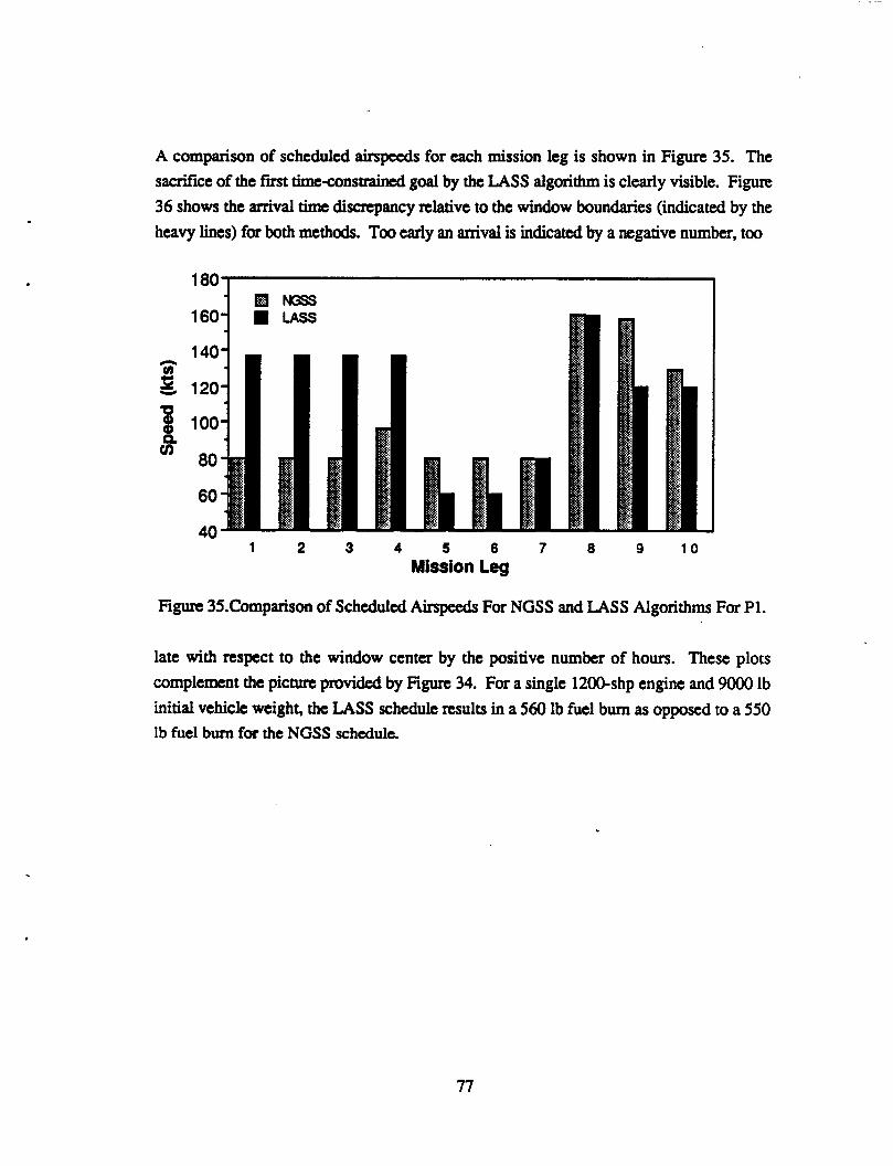
A comparison of scheduled airspeeds for each mission leg is shown in Figure 35. The sacrifice of the first timc-constrained goal by the LASS algorithm is clearly visible. Figure 36 shows the arrival time discrepancy relative to the window boundaries (indicated by the heavy lines) for both methods. Too early an arrival is indicated by a negative number, too

180 m -

l6O1 - 1 2 3 4 5 6 7 8 9 10

Mission Leg

Figure 35.Comparison of Scheduled Airspeeds For NGSS and LASS Algorithms For P1.

late with respect to the window center by the positive number of hours. These plots complement the picture provided by Figure 34. For a single 1200-shp engine and 9O00 Ib initial vehicle weight, the LASS schedule results in a 560 Ib fuel burn as opposed to a 550 Ib fuel burn for the NGSS schedule.

77

Figure. 36. Satisfaction of Time Constraints By NGSS and LASS Schedules For P1.

In the next example, problem P2, the goal distances and wind directions are the same as in the first case, but the wind magnitude is increased to 35 knots and the time window constraints arc shifted slightly with respect to the fmt case. Since the initial timeline (is.* time window constraints) is laid out with a zcro wind assumption for these problems, the high wind speed makes the scheduling problem particularly challenging. The distance versus timc trajectories plotted in Figure 37 far NGSS and LASS algorithms appear quite similar. On closer inspection, it may be observed in Figure 39 that both schedules achieve goal #3, but that only the LASS algorithm successfully captures goals #6 and #8. The NGSS algorithm fails because it does not recognize that adverse wind conditions on subsequent legs require time to be banked on the leg between goals #3 and #4.

78

-1001 J

80 - E S 60-

8 5 40-

n 20 -

n

CI u) -

0 : I I I I

0.0 0.2 0.4 0.6 0.8 1 .o Arrival Time (hrs)

Figure 37.Goal Arrival Times For NGSS, LASS and Specif~ed Constraints For P2.

1 2 3 4 5 6 7 8 9 10 Mission Leg

Figure 38.Comparison of Scheduled Airspeeds For NGSS and LASS Algorithms For €2.

The greater stability in scheduled airspeeds for the LASS speed schedule relative to the NGSS schedule is illustrated in Figure 38.

79

n

S E Y

- g -0.01 -, .II L

0.04 I

Figure. 39. Satisfaction of Time Constraints By NGSS and LASS Schedules For €2.

The last example, problem P3, includes four constraint goals (#s 2,4,6 and 8) and five (non-contiguous) NOE mission legs (#s 2,3,6,7 and 9). The goal distances and winds arc somewhat different than for the first two problems. The NGSS algorithm fails to achieve arrival times within constraints at goals #2, 6, and 8. This is most clearly visible in the arrival time discrepancy plot of Figure 42. The LASS algorithm anticipates the slower mission progress on future NOE legs and banks time on contour flight segments to balance the slower speeds. The LASS arrival time discnpancy was near zero for all four constraint goals in this problem.

80

Q C Y

8

6

C 0 v) CI

80

60

40

20

0 : I I I I

0.0 0.2 0.4 0.6 0.8 1 .o Arrival Time (hrs)

Figure 4O.Goal Arrival Times For NGSS, LASS and Specified Constraints For P3.

1 160

n 140 5

120

100

80

60

40

UI

u)

1 2 3 4 5 6 7 8 9 10 Mission Leg

Figure 41.Comparison of Scheduled Airspteds For NGSS and LASS Algorithms For P3.

81

1 2 3 4 5 6 7 8 9 1 0 Mission Leg

Fig. 42. Satisfaction of Time Constraints By NGSS and LASS Schedules For P3.

The computation times for the NGSS and LASS algorithms arc 0.2 and 1.3 seconds, nspectively on the Macintosh Plus microcomputer for the first two problems, and 0.2 and 1.5 seconds for the last example. Although this represents a significant fraction of the t i m allocated for far-field planning (when 200 candidate plans are considered on a 1 .O Mips processor), the computation time should be manageable within the overall time budget.

4.4

Planned arrival times will not be achievable with open-loop control. The execution component of speed scheduling is necessary for compensation for actual versus planned winds, threat encounters, navigation, etc. The pilot speed advisory can be computed from the ratio of the "distance to go" to the next waypoint and the "the to go" (scheduled arrival time minus current time). This mechanism can be quite simple because a situation assessment function is using the vehicle weight model and associated inputs to regularly update predictions of total resources and time expended during the mission. The thresholding of the difference between the current prediction and the planned value provides the basis for triggering in-flight far-field replanning. This monitoring capability prevents the execution speed scheduler from commanding excessive and futile expenditure of resources before far-field replanning can address the underlying problem at a higher level. It might also be noted that situation assessment will trigger replanning when

82

resource expenditures are substantially better than planned so that far-field replanning can take advantage of new opportunities.

Given a scheduled arrival time at pverv waypoint from the arrival time scheduler (even though only one or two goals may have time constraint specifications), the speed control algorithm has three steps:

calculate quircd ground speed based on estimated position and time to go until

convert to airspeed apply vehicle maximum and minimum spceds to bound the commanded (setpoint)

arrival time

airsped

The equation for the first step is: (SF) (Dta

go vs =

w h m

Vg =groundspeed

SF Dm go =distance between estimated cunrtnt position

Tm go = time interval between ament time and arrival

= safety factor (- 1.05)

and next waypoint

time scheduled for next waypoint

If the time to conduct a search and "homc-in" on the waypoint location to within the specified tolerance is a non-negligible fraction of the transit time, then the factor Tto must include allowance for this starch time. If Tt, go is negative, indicating that the current time (plus search time) exceeds the scheduled arrival time, then the spced for the remainder of that leg is set to the nominal airspetd for that flight mode.

The safety factor (SF) with value slightly greater than unity results in slightly higher speeds on the initial portion of each leg that gradually decrcase along a nominal, uneventful track. It provides an extra margin of time control to counteract the effects on arrival time of unplanned or off-nominal circumstances. The cost of this extra margin is a slightly higher fuel use.

The conversion to airspttd in the second step is given by:

83

where

Va VW =windspeed

= airspetd cmsponding to ground speed Vg

= ground track azimuth %! b =winddirectionazimuth

The third step is represented by:

where vmax

Vmin

V& set

= maximum airspeed for vehicle weight, attitude of

= minimum ampeed for vehicle weight, altitude of

= resultant set-pint airspeed advisory

segment

segment

The values of Vmh, V-, and the range-optimal airspeed may be obtained from previously implemented functions or from an interpolation procedure.

4.5

The primary function of situation assessment is to monitor the execution of the current mission plan and trigger a replanning event when there are indications that the current plan is becoming untenable and also when then arc new opportunities that may be realizable through replanning. The kinds of information available to situation assessment are the time and fuel remaining at selected locations such as waypoints/goals, or alternatively, the distance and fuel remaining at selected times. In prior incarnations of planning, the utility evaluator could be initialized at an arbitrary location in the plan and the current plan utility would also be available as a monitarcd variable.

Given the current planner structure, the distance and fuel remaining at selected times are the p r e f d monitor variables. This does not require the attainment of locations that

84

may be unaccessible by virtue of conditions that are not known a priori in the on-board database or models. The discrepancy between modeled and predicted performance and actual Pcrfonnance, as well as statistical variability in the environment will be the principle challenge to successful execution of a mission plan. Situation assessment and on-board replanning arc critical to meeting this challenge. Situation assessment must trigger replanning with enough lead time so that replanning can be effective in revectoring and reconfiguring the mission for a changing environment. On the other hand, if situation assessment is "hair-triggered," or set off by measurement noise, then replanning at too frequent intervals may preclude the successN execution of any plan.

One concept for mechanizing situation assessment is to calculate position and fuel milestones in the far-term planner and include this information in the mission plan to be passed to situation assessment. The latter would then periodically compare estimated position and mcasured fuel remaining with interpolation between milestones and apply a threshold to the discrepancies to trigger replanning. This concept has several deficiencies, the principle one being the potential inconsistency between planner models and data and the (simulated) "real world." It is not likely that the assumed and "real" drag coefficients and specific fuel consumptions, for example, will be a close match to the real data throughout the mission. Such discrepancies do not necessarily detract from the usefulness of these mociels/data for planning. F O ~ plkning purposes, it is only necessary that the mociels/ciata provide a consistent relative evaluation of different candidate plans and that consistency with respect to the "real world be present in some integral or global sense.

85

A simpler and mom robust schema for situation assessment is to analytically predict the fuel use and final time for the entire mission. These quantities are calculated and saved in situation assessment when a new mission plan is installed. They are then periodically recalculated, used to update a recursive filter estimate, and the filter estimate thresholded against the prediction at plan installation. The fuel used wil l depend on the spetd control and so situation assessment will predict fuel use using the speed control model actually implemnted in the near-field planner. The quantities needed for the prediction are:

currcnt vehicle weight, altitude and time

ground track distance, scheduled arrival time and altitude for all remaining waypoints/goals

wind magnitude and direction for each remaining segment (average)

weight-altitude interpolation of (air density, vehicle speed envelope plus range- optimal specd) and vehicle fuel consumption models.

The analytic solution for the fuel consumption along a mission leg is discussed in Section 5. The fuel use rate is fitted to a linear function of vehicle weight for each mission segment. This is an excellent approximation, and leads to analytically simple results.

The calculational steps for the fuel and time prediction are as follows: initialize TmW to the current time, WGTl to the currcnt weight

for a l l remaining mission legs:

- evaluate Dt, go, the distance remaining on this leg

-evaluate Ttogo =Tscheduledanival- Tnow

- evaluate desired ground speed Vg from Equation (23).

- convert to airspeed and bound by vehicle envelope as indicated earlier in discussion of speed control. Va = commanded airspeed

- evaluate power nquircd and fuel burn rate at WGT1, and at altitude for this leg and speed Va

- extrapolate weight to the end of the leg: W G W = WGTl - (fuel ratel) Tw go

-evaluate power required and fuel burn rate at WG-

- linear fit of fuel burn vs weight: - %= A W + B

86

fuel ratel - fuel rate2) (WGTI - WGTC9) A =I

B = .5[ (fuel ratel + fuel raw - A( WGT1+ W G m ) ]

- evaluate analytic solution for wight at end of leg

- update TmW and WGT1 for next leg

The rtcursive filter equation is:

when e.&.> indicates the filter estimate at the kth data sample WGTkfinal indicates the analytic prediction at the (kth data sample)

and c - .7 to yield a long filter time constant. Cumnt time

The exponential tcrm in Equation 29 can usually be replaced by the fmt ordcr expansion. Then is an identical equation for the final elapsed mission time. The sample (i.e., update) time inmal would probably be on the order of 30 seconds.

The thresholding of the filter estimates with the initial data at plan installation is a test on absolute value of the difference of the quantities. The determination of an appropriate threshold value will require some trial and error, but a value between 3% and 5% is probably appropriate. In some cases, a scheduling of this threshold with mission time may lead to improved pcrfomance with respect to false negative and false positive indications that rcplanning is desireable.

In summary, the concept for situation assessment is not sensitive to early and late errors in individual waypoint arrival times that may cancel through the effects of speed control. The impact of speed control on fuel useagc is explicitly modeled. The updates to the final fuel and time use include the measured (estimated) fuel remaining and vehicle position. Hence, discrepancies between the initial data (at plan installation) and later filter estimates reflect discrepancies between initially predicted and actual fuel and time

consumption. The assessment process should not require any substantial processor time. Finally, the effects of a failure affecting fuel use and timeline such as loss of one engine, the effects of extraordinary winds and the effects of unplanned delays should all be manifest in the monitored variables. The scheme will &tat slow drift in modeled versus "nal world" discrepancies as well as the sudden appearance of such discrepancies.

88

SECTION 5

MODELS

5.1 Backmound

In this section we describe the principle models that support the goal and waypoint- path planners and the testing (simulation) environment. In all instances, the models are used in non-real time to initialize databases that are subsequently used during on-board replanning. In some instances, the models are used in real-time by situation assessment and goal-planning functions. The fuel use model is the most readily derived from phenomenological rotorcraft "theory" and is one of the most important models. Survivability modeling is equally important, but is not deducable in as generic a form as the fuel use model. Finally, there is a brief discussion of the navigation error model and a windfield model. These models have not been integrated with the goal and waypoint path planners during the current phase of this project. Upon integration, all of these models will affect the utility (objective function) evaluation and some will be utilized by the heuristics as well.

89

5.2 Fuel-Use

The fuel usage determination for a given flight path, x(t), may be broken up in four steps as follows:

(1) Determination of the non- gravitational force , E

This follows from the path acceleration, (t ), needed on the flight path with _F (t)

given by ..

EO) = m ( t ) * ? m - g (3 1) where

m = mass of the vehicle g = gravity vector.

(2) Determination of rotor thrusts &

Rotor thrusts for the force and moment balancing requirements are such that :

- F(t) = & + & (32)

where = non-rotor (and nongravitational) force

5 = rotor thrust

Further assumptions are needed on the directionality of TA to help determine TR, given E. We shall assume a flight attitude such that non-rotor aerodynamic force is primarily drag with negligible components along the lift axis and the lateral axis. Above implies that all turning motion is coordinated with zero side angle of attack.

Since Tq is not actively controllable, it can be determined as a function of the flight condition and the airfrsune characteristics.

(3) Determination of rotor power *Pmr

Rotor power to generate the main and tail rotor thrusts for a given flight condition and airframebtor characteristics.

90

(4) Fuelflow rate , WF,

Fuel flow rate required to supply the rotor power and the auxilliary power based on the engine fuel- power characteristics.

We shall now elaborate further steps (2), (3) and (4) above.

5.2.1 Rotor Power Determination

The power applied to the rotor is dissipated in performing three different functions:

(1) inducing a change of momentum in the air mass flowing through the disc of the rotors, with power expended, Phd , "induced power."

(2) moving the blades through the moving air, i.e. overcome the rotor drag, with power expended, Pprof, "profile drag."

( 3 ) overcoming the parasitic drag associated with the movement of the air past the non- rotor components, with power expended termed, PPm , parasitic power.

Analytical modelling of the airflow is difficult in the face of important effects such as stalling, compressibility etc. A simpler approach based on momentum and blade element theories is favored [15]. Further, the rotor power, Pmmr, is determined for level flight with additive corrections for changing the energy-level [ 161, i.e.

protor = Plevel flight + PAenergy level (33)

91

with flight in horizontal plane at unchanging energy-level, Es, defined by:

where h = altitude W = weight I = rotorinertia

R = rotor speed v =airspeed

The power required to change the energy-level may be determined from (34) , viz.

dEs dh+vdv I Q d n dt dt gdt W dt - = - -- +--

and the relationship W d B

PAenergy level = &

(35)

where n is the efficiency factor. Of particular interest are the two cases with reported values of climb/descent and level acceleration with values of n as below:

- climb/descent condition [15]:

n = .75 - 3 5 for dh/dt > 0 = 1 for BNdt c 0 (37)

- level acceleration [ 161 :

n = 0.8 - 1.0 (38)

The power required for level flight is calculated in terms of the three components described earlier:

Plevel flight = P i d + Pprof + ppara (39)

We give below the detailed equations of the three components:

Rotor induced power, Pid

Pid = Tm Vi

where

Tm = rotor thrust (based on earlier steps 1 and 2)

92

= induced velocity given by Equation (41)

1 m r (the induced velocity at hover) (42)

2p~Rmr*E~

=0.95 [15]

= main rotor radius

(effective non-dimensional rotor radius where tip losses become significant)

= air density = vehicle forward air speed

Rotor blade profile power, Ppmf

where

(rotor solidity ratio) bc ZRmr

CJ = -

b

C = blade chord

= number of rotor blades

- q = blade section drag coefficient

p = - (rotor advance ratio)

vt = tiprotorspeed=QR,

V "I

Typical values for these parameters are: - cd = 0.0()8 (main rotor)

= 0.0107 (tail rotor)

93

Parasitic Power, Pm

where

fe = equivalent flat plate area of non-rotor drag

Typical Values: From Figure 1.4 of [15], we have following trend values for production helicopters:

= 200 lbs/ft2 for high drag designs

= 400 lbs/ft2 for average drag designs

= lo00 lbs/ft2 for exceptionally clean designs

Additional gects:

It may be remarked that effects such as the non-uniform downwash effect, compressibility effect, parasitic power correction,etc. give rise to corrections to the expressions above. These corrections, however, are higher order (and hence negligible) terms from the perspective of modelling for fuel-use planning.

Tail Rotor Power, Pt,

As described earlier, the tail rotor thrust, Tt,, is determined h m moment balancing considerations , specifically to overcome the main rotor toque. Thus,

(45) Pmr Tw =

Qmr&

where Pmr = main rotor power, ft-lb/sec

Qm = main rotor speed, radsec

Lt, = tail rotor moment arm, (ft).

94

Shaft Power, Psh

Having determined the main and tail rotor power requirements for a given flight condition as above, we can determine the required shaft power at the engine from

The tail rotor power, Pm, requirements are detemined from [ 151

(46) Pu =Tt ,Vie+gOmEdJ 1 1 +4.7 ~ ~ 2 ) p x R ~ 2 ~ t ~ ’

where Vi follows from equations of the same form as (41) and (42) with Tm and Rmr of (42) replaced by Tt, and Rt, associated with the tail rotor and pu and vt are defined similarly.

where nt = transmission efficiency

APXc = accessory losses

We can express the shaft power conventionally in terms of hp units with Psh 5 5 0 (hp) (48) SHP = -

Typical Values [ 151:

nt = 0.95 for low and intermediate speed bevel and planetary @ars

= 1.0 for high speed bevel gears and

APzc = 2 9% of shaft power, related to engine plus transmission cooling blowers, electric power generators and hydraulic power supplies.

95

5.2.2

of

Engine Fuel Flow Model

Engine rating

We size the engine with maximum continuous rating at sea level standard conditions

SHP,c = k P ( hover, sea level std, max wt) (49)

where k = factor > 1.

For the utility/transport type helicopter of [ 151, k = 1.04. For an agile attack helicopter, a more appropriate choice is k = 2.0. The second factor represents the shaft power required for hover at sea level and standard day temperature, pressure and density conditions and maximum weight conditions as evaluated from Equation 48. A higher power level called the "intermediate continuous" power ( S H P I C ) is available for a limited stretch of time (no more than 4 hrs, [ 151) for takeoff or emergency situations. A typical ratio [ 151 for SHPIc /SHPMC = 1.23. Both power ratings change with pressure altitude and ambient temperature as:

SHP, = S H P O 6 + i

where

SHP, = engine rating at sea level standard atmosphere

6 = ratio of ambient pressure to sea level std pressure

8 = ratio of sea level std absolute temp to ambient temperature

The engine rating for different vehicles may be specified to support hover requirements at higher altitudes, hotter ambient temperatures, or to support maneuver requirements.

Fuel Flow Model

Given the required shaft power, SHP as per Equation (48), we can determine fuel flow rate , WF , from the engine characteristics. We shall assume an engine with Specific

- fuel consumption, (sfc 2 WF/ SHP) characteristics as given in Figure 1.8 of [15], that also reflects the sfc trend of typical engines with sfc = .5 lb/hp-hr at the design cruise condition.

96

Based on Figures 1.8 and 1.9 of [15] , we can determine the following fuel flow model:

096 S H P sfc = 0.404 + .+

WF = 0.404 S H P + 0.096 SHPIC (52)

5.2.3 Selection of Hypothetical NOE Mission Helicopter Parameters

We have chosen many parameters from standard design considerations and from [ 151. We still need to determine the basic rotor parameters of solidity, rotor radius and rotor speed along with the weight of the vehicle. This will then complete the specification of all parameters that are of significance for fuel flow modelling.

The prominent considerations for the selection of rotor parameters may be simply stated as below.

- rotor radius , i.e. disc loading, is selected large enough such that disc loading and hence induced power losses are low. It may be remarked that induced power at hover primarily determines the size of the engine and hence the fuel load required for a given mission, with lower disc loading leading to improved fuel-to-weight ratio.

- rotor speed/solidity are selected to minimize the rotor blade profile power based on minimizing the rotor tip speed subject to stall angle limitations. The minimum profile power loss is achieved for blades operating, on the average, at as high an angle of attack as is possible without stalling and such that the requisite thrust is produced. The tip speed is selected based on stall and compressibility considerations at maximum forward speed

whereas the solidity is picked from power efficiency considerations.

The NOE mission hypothetical helicopter parameters for fuel flow modelling purposes are as below:

Weight Parameters

Design gross weight = 7500 Ibs

maximum weight = 1.2 7500 lbs , using same fraction as in [15].

97

Rotor Parameters

I MainRotor I I

I 20 ft 28 radsec

4 0.75 ft

Parameter Tail Rotor

3.5 ft 28 radsec

4 0.75 ft 23.5 ft

radius R rotorspeed R no of rotors b rotorchord c momentarm LW

Table 3. Rotor Parameters For Baseline Helicopter Model

The rotor radius is sized so as to provide rotor loading, , defined as rotor thrust (hover) t c = (53)

P V t L rotor area 0.7

of approximately 0.3 ( see [ 16 1, also [15] helicopter has the same value). Further we select the same rotor speed, and same type of blades as [ 151.

Calculation of lift required for turning-climbing flight

We shall consider the case of a coordinated turning-climbing flight at unchanging speed. The figure below defines the forces on the point-mass model vehicle. The required lift for the coordinated turning-climbing flight at unchanging speed can be determined from the steady state equations of motion in the lateral as well as longitudinal plane.

98

4 A L cos & cos $

Lift vector L

I LsinE Longitudinal Axis

L cos & sin $

~~

Figure 43 Lift Vector Components Along Longitudinal Axis And In Lateral Plane

In the lateral plane, the lift components are required to overcome the component of gravity as well as provide turn acceleration. Thus,

mgcosy = LCOSECOS$

mri$ = LCOSESin$

where

E

y $ =bankangle r = turningradius,

y/ = turnrate = v c o s y / r

= angle of tile of lift vector out of lateral plane

= flight path angle (positive is climbing)

(54)

(55)

.

99

In the longitudinal plane, the lift vector is tilted by E to overcome drag and the component of gravity along the longitudinal axis. Thus:

L s i n ~ = D + mgsiny (57)

Combining equations (54) and ( 5 3 , we may derive:

L cos E = -\I cos*y+ r i 2 - mg g

From (27) and (28) , we can determine the required lift ( Le. the rotor force ) with

Given the vehicle forward speed, the net drag force D is estimated as:

fte P v2 2 D =

where fE = equivalent flat plate area for total drag

After adding the wind velocity to derive an inertial velocity, vi,,, and given a rate of climb, k , the flight path angle is inferred:

(61) il siny = -

vin

- G2 Hence, given the flight conditions of altitude, speed, climb rate, and g (the number of g's pulled in turning maneuvers), Equation (59) can be evaluated for the rotor thrust required for that flight condition. Equations (39) through (48) are then evaluated for the power required and equations (35) through (38) are applied for the energy-state correction, PAenenrgy level.

The following figures illustrate the power and fuel rate trends as a function of vehicle weight and airspeed at different flight conditions. Figure 44 shows the power required, fuel rate for an assumed engine rating, and fuel economy as a function of airspeed

.

and vehicle weight. The boundaries of the shaded regions correspond to the 6000 and 7500 Ib vehicle weights for level flight. The minimum fuel rate occurs at a slightly higher airspeed than the minimum power requirement. The maximum "fuel economy" in terms of distance travelled per pound of fuel consumed occurs at a still higher airspeed. The variation of the lower curves is somewhat suppressed by the scaling, but the fuel economy is slowly varying over the high speed region above 150 ft/s. The variation with vehicle weight (Le. across the shaded areas) at a given speed is highly linear over the indicated load range.

800 I 1

600

400

200

0 onomy ( d b x 200)

0 50 100 150 200 250

Airspeed (ft/s)

Figure 44 Power, Fuel Rate, and Fuel Economy For Vehicle Weight 6OOO - 7500 Ibs.

The next figure shows the variation of power requirement with vehicle weight and airspeed for a level turn at 2G turn acceleration at sea level compared to the level flight power requirement at the same conditions. The shaded region again represents the variation with vehicle weight. The fuel use rate and fuel economy show similar parametric variation with flight conditions and vehicle weight.

101

2500

2000

1500

1000

500

I I I I

0 50 100 150 200 Airspeed (ft/s)

Figure 45. Power Requirements For Level Flight and 2G Maneuvers (Sea Level Std.)

Finally, Figure 46 shows the power requirements for flight conditions corresponding to two different climb rates in the same format as the previous figures. The power and fuel use for any combination of altitude, airspeed, climb rate, turn acceleration, and vehicle weight can be obtained from the models described in this section.

In order to use all of the above in planning, it is first necessary to establish a correspondence between terrain features at the underlying map resolution (-2 km) with a program of flight conditions (t ) for each of several flight modes, including NOE, contour flight, and cruise. For example, the program of flight conditions in traversal of any grid box must be summarized as a function of a few parameters that distinguish one grid box area from another. The fuel-use models are used with the assumed flight conditions to infer the fuel use in traversal of each category of grid box, or possibly for each grid box. These calculations are performed preflight and are part of the preparation of the database that is used for planning. Parameters are stored for each grid box that can be used in the on-board planning process to evaluate the fuel-use in traversing that grid box as

102

a function of speed, direction, and flight mode. The software and methodology for preparing this database have not been addressed in the f ist year's effort as currently reported.

1500

-

1000

500

I I I

100 150 200

Airspeed (ftls)

Figure 46. Power Requirements For 20 and 40 ft/s Climb Rates (Sea Level Std) Upper and Lower Boundaries of Shaded Regions Correspond To 7500 and 6OOO lb

Vehicle Weights, Respectively.

5.3 Survivabilitv

The basis for waypoint planning is the network search for a minimum cost (lethality) path subject to a resource constraint. The path costs are assumed to be additive over the nodes that are traversed. The path cost reflects the impact on survivability for transit between nodes of the nctuork. Detailed and high-fidelity modeling of threat engagement and outcomes is not s o important for path determination as the expression of relative cost between alternative paths.

From an intutitive basis, i t is to be expected that the lethality cost per unit time (or

103

distance) will be a function of the vehicle location, flight mode (Le., NOE or contour), and vehicle speed. The location dependence arises from differences in terrain features that reflect the vehicle detectability in different flight modes. For example, at several hundred feet altitude over flat terrain or water, the vehicle is detectable at great distances by ground- based radar and electrooptic sensors. When there are terrain features such as trees and hills and the flight mode is NOE, vehicle detectability can be made quite small by using intervisibility constructions to provide terrain masking between vehicle and (known) threat emitters. The location-dependence also derives from the number (or number-density) and type (i.e., capability) of threats and their geographic distribution. The vehicle speed influences the lethality cost because the dwell or exposure time within threat range is inversely proportional to the vehicle speed. Slow speeds permit more time for acquisition, targeting, and weapon employment against the vehicle. This holds true for infantry small arms fire as well as surface to air missiles.

The comct functional trends for lethality cost should be produced by the following model:

where

x = detection rate per unit time

At = transit time from node i to node j

co = normalization constant

For a given threat environment and flight mode, the cost is an exponentially saturating function of exposure (transit) time between nodes. The detection rate, a, will depend linearly on the known threat density or probability of their being a threat of a given type within detection and engagement range of the nodal segment. The exposure time can be converted to a distance as:

As At = - V

where

As = internodal distance

V = average ground track speed

Finally, the terrain will influence h by intervisibility considerations and multiple

104

threat types can be separately enumerad

where

h m = detection rate per unit time for threat type m

PT = threat density per unit area

R = local topography

The speed to be used in Equation (64) is a nominal vehicle speed for the flight mode indicated for that node. The flight mode is determined by the density and capability of threats in the mission area. Contour flight is preferred in lower risk areas to minimize flight time, pilot and vehicle stress and fuel use. NOE flight is indicated when the assessed risk exceeds a certain threshold and low, slow and concealed transit is preferred.

The exponentially saturating model is appropriate to a random encounter model wherein threat locations are not precisely known, or are known only probabilistically as density functions. Assuming a detection range, distribution of threats, and a detection model involving coherent integration of information received over a period of time, the detection rate h can be derived phenomonologically. It is sufficient for our purposes, however, to assume that there is some known function hm(pTp ) that can be evaluated to yield lethality costs for transit between all pairs of adjacent nodes. This information is processed preflight and results are stored in an array to support waypoint path planning. The cost numbers may not be in a form easily relatable to quantitative survivability, but they are nonetheless useful in evaluating different paths for cost-incurred versus resource- used tradeoffs. In addition, the goal planner will use the cost information (and possibly

other information stored for the network) to evaluate the branching probabilities discussed in Section 2.

5.4 Navigation Error

A navigation error model is to be used by the goal planner to assess the probability of achieving goal arrival within specified positional tolerances and to assess the time and fuel-use needed for landmark search to support a navigation update. These considerations will affect the evaluated utility for any mission plan and will indirectly affect the converged mission plan when the effects of navigational uncertainty cannot be assumed to be

105

negligible. Some goals and associated goal actions will require tight positional tolerance whereas other goals need not be overflown to high accuracy, if at all. In general, provision should be made in any planner design to accomodate the real likelihood of navigation errors, navigation uncertainty and navigation requirements.

Without detailed modeling of any particular inertial navigator, the following model captures the essence of the navigation error and uncertainty propogation in time. The velocity errors are assumed to be described by a first-order Markov process:

where

u(t)

z = time constant

= unit variance white noise

ov2 = steady state velocity error variance

Together with the position error equation,

6; = 6v

the coupled system can be written in discrete time form as

where

6P(O) - N(O,OpO*)

6 ~ ( 0 ) - N(0,0a2) ul(t),u2(t) = unit variance, zero mean, independent

sequences of white Gaussian noise

a(At) =

b(At) =

d(At) =

106

.I

The covariance is ppogated as:

in between landmark updates, and

after the update. Numerical examples of the evaluation of the above model are shown in Figures 47 and 48. In the first figure, the positional enor trajectory is plotted at a number of discrete time points, showing the meandering growth of positional error (without navigation updating). In Figure 48, the positional error is plotted as a function of time along with the ? lo error position uncertainty from the covariance equation.

107

-1 5000 -1 0000 -5000 0 X-Position Error (ft)

Figure 47. Position Error Trajectory For First-Order Markov Process.

0 20 40 60 80 Time (min)

Figure 48. Position Error And I 'ncenainty (Covariance) Without Landmark Updates.

108

5.5 Windfield Model

The prevailing winds as a function of altitude, month and location may be predicted by use of semi-empirical models and an associated database [18,19]. The basis is the geostrophic wind relation:

1 a p v = 2 p o s i n ~

where

U

V

P = atmospheric density

0

$ = latitude

= eastward (horizontal) wind component

= northward (horizontal) wind component

= angular velocity of the Earth's rotation

= north component of horizontal pressure gradient ap F ap = east component of horizontal pressure gradient

This relation is valid away from the equatorial belt &e., ? 15' latitude) and for altitudes

from about 1 to 25 kilometers above ground level. It is derived from the force balance between the pressure gradient and the Coriolis effect; and neglects friction, time changes of wind, and vertical motion (usually c .03 ft/s). In a band around the equator, an interpolation scheme between wind values at the boundaries of the band is used to predict wind values inside the band.

In addition to the mean geostrophic winds inferred from the monthly mean pressure and density data, there are corrections for "Quasi-Biennial Oscillations" (QBO) in the pressure, density, temperature, and winds with an 870 day period sinusoidal oscillation and with amplitude and phase varying with altitude and latitude. Also, there are smal l scale random perturbations that represent the effects of turbulence and gravity waves and large scale random perturbations representing tides and planetary waves. The random perturbations are correlated spatially across relaxation distances of several to several tens of kilometers.

109

Data for (monthly mean) pressure, temperature, density, and perturbation (daily) variances are stored in a database containing a total of 3490 latitude,longitude points including the National Meterological Center (NMC) grid, a northern hemisphere equatorial (EQN) grid, and a southern hemisphere (SH) grid, with empirical data for every one kilometer altitude up to 25 kilometers and for every month of the year. An elaborate interpolation scheme is used along with a finite difference approximation of equations (7 1) and (72) to calculate the predicted windfield. The correlations for the random perturbations are also fairly elaborate, and the random contributions are appropriately sampled. Since the variance in the windfield components is typically a good fraction of the mean value of those components, the output windfield is one sample point from a random distribution. If actual meterological measurements are available, however, the windfield model can be used to extrapolate from the measured data out to a distance on the order of the correlation distances.

The windfield model is not obviously useful at NOE or even contour flight altitudes, but may be used nonetheless to generate simulated windfields for testing. The planning database requires terrain, threat (i.e., intelligence), and meteorological inputs arrayed on a common basis and reduced to representations that facilitate rapid access and utilization. The construction of these databases to support operational use of planning software is a substantial task by itself that has been largely ignored to date.

110

SECTION 6

CONCLUSION

6.1 Summary

The major components of a far-field mission planner have been studied and algorithmic solutions implemented in a microcomputer environment. These include a goal planner, waypoint path planner, speed scheduler and associated models. The microcomputer environment was the Fortran language on the Apple Macintosh PlusTM Computer, a 68000-based computer (without math coprocessor) with approximately 0.1 Mips processor speed and with 5 12 Kbytes memory usage.

The overall planning framework for multi-objective missions with multiple constraints is based on a utility theory formulation. That is, the probability of successfully accomplishing each objective given an environment, initial conditions and a mission plan to be followed, is estimated using models for fuel use, survivability, transit time, etc. The overall worth of a multi-objective mission plan, in comparison to other candidate plans, is determined from the product of the probability of accomplishing each objective with the relative value of that objective, summed over all objectives. Constraints may not permit all objectives to be accomplished. Local and global constraints are expressed directly in the

estimated probabilities, and in some instances, in a penalty function that modulates the set of relative values. Examples of such constraints include global constraints on fuel, resources and survivability , and locul constraints associated with time windows, goal ordering and minimum probability of success. Using a generate and test paradigm, the mission plan with the best utility value is constructed. Good mission plan solutions are available quickly in the face of the combinatorial (i.e., factorial) complexity of the problem. The globally optimal solution is frequently obtained within the solution time requirements, but is only guaranteed asymptotically with solution time.

The solution methodology for the goal planner is the heuristically-guided simulated

111

annealing method. The annealing algorithm is a variation on the hill climbing method that permits unfavorable downhill moves (conditionally) so as to avoid the trapping in locally optimal solutions that frequently occur with pure gradient search techniques over objective surfaces. The heuristics are formulated to operate on generic parameters such as relative goal values and normalized resource use (viz a constraint). The heuristics also use a probabilistic sampling technique to avoid limit cycling and to schedule the degree of venturesomeness of the search within the available solution time. In comparison with alternative algorithms for a stochastic travelling salesman problem, the goal planner algorithm outperforms other algorithms based on dynamic programming, multialgorithm heuristics, enumeration, linear programming and expert system approaches. The performance evaluation is based on robustness (i.e., the frequency of obtaining optimal solutions within a given solution time limit), the degree of optimality when averaged over all solutions on a battery of test problems and the time to obtain the optimal solution.

The waypoint path planner supports the goal planner by providing lethality cost, fuel and resource use and transit time for multiple path solutions between each pair of objectives. The multiple solutions are each a minimum (lethality) cost optimal solution subject to different resource constraints distributed on the cost-resource operating curve. The waypoint path problem is formulated as a network search problem and a combination of uniform cost and uniform resource A* expansion techniques are developed to generate the entire cost-resource operating curve and to find paths corresponding to selected points on that curve. The algorithms selected are compared to a dynamic programming approach to network search wherein resource use is identified as the dynamic programming stage variable. The methods selected are shown to be considerably more efficient than the dynamic programming approach for the range of network sizes in the intended application. The technique to generate the entire cost-resource operating curve is a new and significant development. The solution time budget and NOE mission profile seem to indicate that 12Wnode networks with 2 km internodal distance are feasible when computation times are scaled to the target 1 .O Mips processor.

The speed scheduler is the third major far-field planning component and affords flexibility to enable successful completion of downstream objectives with time constraints without massive alteration of the mission plan or sacrifice of goals along the way. The speed scheduler algorithm determines the maximally plan most likely to satisfy respective time constraints.

valued subset of goals in a mission When there is latitude in scheduling

112

an arrival time at a goal that will satisfy all constraints, heuristics are used to select a time aimpoint that minimizes fuel use and maximizes survivability. The approach taken is based on the determination of the back-projection and intersection of speeds required to satisfy time constraints (in a given windfield) within the speed envelope constraints of the vehicle. In both the NOE and contour flight regimes, the speed envelope is determined by the balance between survivability (Le., time exposure to threats) and ground avoidance considerations. Two different speed ranges are postulated for missions encompassing a mixture of both NOE and contour flight mission segments. The algorithm ("LASS" algorithm) is compared to a simpler algorithm that schedules speed to the next constraint goal without any look-ahead or consistency checking with regard to multiple constraint goals ("NGSS" algorithm). A number of random scenarios are generated and it is easily seen that the LASS algorithm far surpasses the NGSS algorithm in its ability to schedule speeds that satisfy time constraints given mission time changes (i.e., delays or advances) and unexpected wind conditions.

Finally, preliminary modeling was performed to support fuel use and lethality cost predictions that are made in constructing the databases used by the planning components. Given the basic helicopter parameters such as rotor parameters, engine rating, etc., the fuel use can be estimated for any combination of weight, altitude, speed, lateral (turning) acceleration and rate of climb.

6.2 Future Work

Substantial development and integration activities remain to be accomplished. Although the database that each of the far-field planning components operate upon is well- defined functionally at this point, the software design for the databases in an integrated planning system remains to be evolved. Another large task involves the construction of the network database from the application of models to an underlying database of terrain, threat and weather parameters. Although much of this will be performed preflight in any operational system, there remains 3 rrsidual need for an on-board capability for that portion of the underlying database that is updated by sensors or communications.

As a subtask related to the construction of planning databases from mission environment databases, there mu\[ be further work to relate the NOE and contour flight

113

profiles to the variables of the fuel-use model as a function of the underlying terrain. Also, the lethality cost model needs to be fleshed out with information relevant to survivability in low-level helicopter operations.

The integration of far-field planning with any mission management executive requires the development and testing of a (far-field) situation assessment module. This function will trigger far-field replanning to respond to departures from nominal plan execution that have time, fuel-use and survivability impacts. The situation assessment function will also respond to communications that change objectives, objective values and environmental features.

Upon testing of an integrated far-field planning system within its own test environment, the next step is to begin integration with near-field planning and with simulation and test facilities such as the NASA Ames Crew Station Research and Development Facility. Among other tasks, it is at this point that man-machine interface issues will need to be addressed. It is anticipated that there will be much useful feedback from pilots to mission software developers and that mission planning software will be used in ways that are not easily forseen by those developers.

.

114

REFERENCES

.

1. "Research and Technology Annual Report - 1986," NASA Ames Research Center, Moffett Field, California, NASA TM89411, April, 1987.

2. O.L. Deutsch, J.V. Harrison, M.B. Adams, "Heuristically-Guided Planning For Mission ControlDecision Support," Proceedings of 1985 AIAA Guidance, Navigation, and Control Conference, Snowmass, Colorado.

3. R.V. Denton, J.E. Jones, and P.L. Froeberg, "Demonstration Of An Innovative Technique For Terrain Followinflerrain Avoidance - The Dynapath Algorithm," Proceedings of the IEEE Natl Aerospace & Electronics Conf, May 20-24,1985, pp 522-529.

4. O.L. Deutsch, "The AI Design Challenge - Background, Analysis, and Relative Performance of Algorithms," Proceedings of 1987 AIAA Guidance, Navigation, and Control Conference, Monterey, California, pp.465-476.

5. S. Kirkpatrick, C.D. Gelatt, and M.P. Vecchi, "Optimization by Simulated Annealing," Science, Vol. 220, May 13,1983, pp 671-78.

6 . D. Mitra, F. Romeo, and A.S-Vincentelli, "Convergence And Finite-Time Behavior of Simulated Annealing," Proc. 24th Conf. on Decision & Control, Ft. Lauderdale, Florida, December, 1985, pp. 761-766.

7. L.L. Carter and E.D. Cashwell, Particle-Transmrt Simulation with the Monte Carlo Method, U.S. Energy Research and Development Administration (TID-26607), 1975, pp. 13-16.

8. J. Spanier and E.M. Gelbard, Monte Carlo Princbles and Neutron Transport Problem$, Addison Wesley Publishing Co., 1969, pp. 101-109.

115

9. E. Bonomi and Jean-Luc Lutton, "The N-City Travelling Salesman Problem: Statistical Mechanics and The Metropolis Algorithm," SIAM Review, 26,551-568 (1984).

10. F. Romeo, A.S. Vincentelli, and C. Sechen, "Research on Simulated Annealing at Berkeley," Proc. IEEE Int. Conf. on Comp. Design, pp. 652 -657, October, 1984.

11. B. Hajek, "A Tutorial Survey Of Theory And Applications Of Simulated Annealing," Proc. 24th Conf. on Decision and Control, pp. 755-760, Ft. Lauderdale, Florida, December, 1985.

12. H.H. Szu, "Non-Convex Optimization," SPIE Roc. Real Time Signal Processing IX, Vol. 698, 1986, pp. 59-65.

13. J. Pearl, Heuristics - Intellige nt Search m e s for C o m Problem Sol ving, Addison Wesley Publishing Co., 1984, p. 64.

14. S. Green, T. Davis, H. Erzberger, "A Piloted Simulator Evaluation of a Ground- Based 4D Descent Advisor Algorithm," Proceedings of 1987 AIAA Guidance, Navigation, and Control Conference, Monterey, California, pp. 1173-1 180.

15. C.N. Keys , "Rotary Wing AeroDynamics, Vol 2: Performance Prediction of Helicopters," Final Report (Boeing Vertol Co., Philadelphia, Pa.), CR-3083, 1979, NASA.

16. C.D. Wells, T.L.Wood , "Maneuverability-Theory and Application," 28th Annual National Meeting AHS, 1972.

17. W.Z. Stepniewski, "Rotary Wing Aerodynamics, Vol 1," CR-3082, NASA.

18. D.B. Spiegler and M.G. Fowler, "Four Dimensional World-Wide Atmospheric Model - Surface to 25 Km Altitude," CR-2082, July 1972, NASA.

19. C.G. Justus, G.R. Fletcher, F.E. Gramling, and W.B. Pace, "The NASA/MSFC Global Reference Atmospheric Model - MOD 3," CR-3256, March 1980, NASA.

116

Report Documentation Page 1. Report No.

NASA CR 177482

4

2. Government Accession No. 3. Recipient's Catalog No.

4. Title and Subtitle

DEVELOPMENT AND DEMONSTRATION OF AN ON-BOARD MISSION PLANNER FOR HELICOPTERS

5. Report Date

MAY 1988

6. Performing Organization Code d 7. Author(s) 8. Performing Organization Report No.

OWEN L. DEUTSCH MUKUND DESAI

9. Performing Organization Name and Address

CHARLES STARK DRAPER LABORATORY, INC. CAMBRIDGE, MA 02139

12. Sponsoring Agency Name and Address

NASA AMES RESEARCH CENTER M.S. 210-9

CSDL-R-2056

11. Contract or Grant No.

NAS2-12419

13. Type of Report and Period Covered

CONTRACTOR REPORT

14. Sponsoring Agency Code

17. Key Words (Suggested by Author(s)) NOE FLIGHT, MISSION MANAGEMENT, FAR-FIELD PLANNING, CONSTRAINED OPTIMIZATION, GOAL PLANNING, WAYPOINT PATH PLANNING, TIMELINE MANAGE- MENT, SIMULATED ANNEALING

I MOFFETT FIELD, CA 94035

18. Distribution Statement

UNLIMITED DISTRIBUTION

STAR CATEGORY 08

I 505-66-11

19. Security Classif. (of this report)

UNCLASSIFIED

I 15. Supplementary Notes

20. Security Classif. (of this page) 21. No. of pages 22. Price

UNCLASSIFIED 117 A06

POINT OF CONTACT: LEONARD A. MCGEE M.S. 210-9 MOFFETT FIELD, CA 94035 (41J) 694-5443 or FTS 464-5443,

I 16. Abstract Mission management tasks can be disaibuted within a planning hierarchy, where

each level of the hierarchy addresses a scope of action, an associated time scale or "planning horizon". and nquirements for plan generation response time. The current work is focused on the far-field planning subproblem, with a scope and planning horizon encompasing the entire mission and with a response time required to be. about two minutes. The far-field planning problem is posed as a constrained optimization problem and algorithms and structural organization arc proposed for the solution. Algorithms are implemented in a development environment, and performance is assessed with respect to optimality and feasibility for the intended application and in comparison with alternative algorithms. This is done for the three major components of far-field planning: goal planning, waypoinr path planning, and timeline management. It appears feasible to meet performance requirements on a 1.0 Mips flyable processor (dedicated to far-field planning) using a heuristically-guided simulated annealing technique for the goal planner, a modified A* search technique for the waypoint path planner, and a speed scheduling technique developed for this project !