E USCIPI Report 680

UNIVERSITY OF SOUTHERN CALIFORNIA

IMAGE RESTORATION BY SPLINE

N1 FUNCTIONS

by

E Mohammad Javad Peyrovian

E August 1976

Image Processing Institute

R University of Southern California

University Park

Los Angeles, California 90007

N Sponsored by

Advanced Research Projects Agency

Contract No. F-33615-76-C-1203ARPA Order No. 3119

APPROVED FOR PUBUC REto rDISTRIBUTION U: LIMITD

DISTEIBUTION STATEMENT AApproved for public release; I

Diaoulbtion UnlimitedDTIC

U" .',.DEC16 t982~ ZP

iIMAGE PROCESSING INSTITUTE

C2 12 15 101lop

USCIPI Report 680

IMAGE RESTORATION BY SPLINE FUNCTIONS

by

Mohammad Javad Peyrovian

August 1976

Image Processing Institute

University of Southern California

University Park

Los Angeles, California 90007

This research was supported by the Advanced Research

Projects Agency of the Department of Defense and was

monitored by the Air Force Avionics Laboratory under

Contract No. F-33615-76-C-1203, ARPA Order No. 3119.

The views and conclusions in this document are those of the author and

should not be interpreted as necessarily representing the official policies,

either expressed or implied, of the Advanced Research Projects Agency

or the U. S. Government.

UNCLASSIFIED

IOCUMENT CONTROL ATAY R F T D(S c rITV ., hraf-rt OfES(T f epo, bdy 0 bI.elr 0. d a-e -t ht - rd wh- Ih , 1, -p- '

eOR hGIN TING AC l Vl Y (Cur"oraf* auth-) 12a. "t Pow r AuLCju st ( LA',1IFI6A 1 -14UNCLASSIFIED

Image Processing Institute 2b. GRtOnP

University of Southern California, Los Angeles, CA3. RI EPORT TITCE

IMAGE R.ESTORATION BY SPLINE FUNCTIONS

SDE'SCRIP=TIVE NOTES (7)rpe oi report and inclusiv date*)

Tech nica 0eot Ae 1976S. AU THOR|S) " R ;fnn,- middleiiia l, lat nmere)

MVohammrad J. Peyrovrian

5. RFPL,4r )ATE 7.. TO rAL NO. 0I F'A 5 ES b. No vw RE-9

31 August 1976 121 64. CONTRACT OR GRANT NO Qa. ORIGINATOR'S REPORT NUMBER(S)

F-33615-76-C- 1203b. POJECTNO / USCIPI Report 680

c. ARPA Order No. 3119 Bt. O THER REPORT NO(S) (Any other numbers tha may be assignedthis report)

d.

io DISTRIBUTION STATEMENT

Approved for release: distribution unlimited

II. SUPPLEMENTARY NOTES 12. SPONSORING MILITARY ACTIVITY

Advanced Research Projects Agency1400 Wilson Boulevard

' _ _ _ Arlington. Virginia 2220911. ABSTRACT

"VSpline functions, because of their highly desirable interpolating and approximat-

ing characteristics, are used as a potential alternative to the conventional pulseapproximation method in digital image processing. For uniformly spaced knots,a class of spline functions called B-splines has the useful properties of shiftinvariance, positiveness, and convolutional and local basis properties. Theseproperties are exploited in image processing for linear incoherent imaging systems.e;

The problem of image degradation in a linear imaging system is described by a

superposition integral. For simulation of degradation and restoration by means ofa digital computer, the continuous imaging model must be discretized. Thus, atheoretical and experimental study of quadrature formulae, pa"icularly monosplineand best quadrature formulae in the sense of Sard, is presented, It is shown thata good choice of degree for a monospline highly depends on the frequency contentof the integrand, and in most cases, a cubic monospline generates less error thanthe pulse approximation method and Newton-Cotes quadrature formulae.

In space-invariant imaging systems, the object and point- spread function arerepresented by B-splines of degrees m and n. Exploiting the convolutional

property, the deterministic part of the blurred image is a spline function of degreem + n + 1. A minimum norm principle leading to pseudo-inversion is used for the

restoration of space-variant degradations and underdetermined and overdeterminedmodels. Space-variant point-spread functions that describe astigmatism and

DD 1473,% iv tl IV - , %hclldttnrn

14 LJrJ.. A L ' I -it.K

K 0IV VL FR WT "i LO 7. 1 | , RO I

curvature-of-field are derived and coordinatetransformations are applied to redi:ce the dimen-sionality. The singular-value - de compositionechnique is used for solution of the simplified

equations.For noisy blurred images, a controllable

smoothing criteria based on the locally variablestatistics and minimization of the second deriva-tive is defined, and the corresponding filter,applicable to both space-variant and space-invariant degradations, is obtained. The para-meters of the filter determine the local smooth-ng window and overall extent of smoothing, andhus the trade-off between resolution and smooth-ng is controllable in a spatially nonstationary

anner. Since the matrices of this filter areanded circulant or Toeplitz, efficient algorithmsre used for matrix manipulations.

14. Key Words: Digital Image Processing,Monospline Quadrature Formulae,Image Restoration, Spline Func-tions, Smoothing Splines.

- t ---

. .. . ... . ... ...... . ... . ... .. .......... . .... .... .. ......... .. .... ... " I I - I(l . . . .. I I I I I l l

ACKNOWLEDGEMENT

rhe author wishes to express his sincere gratitude to the

chairman of his committee, Professor Alexander A. Sawchuk, for

his guidance throughout the course of this research. Without

Professor Sawchuk's suggestions and encouragement this

dissertation could not have been possible. The author also feels

deep appreciation towards Professors Harry C. Andrews and

John G. Pierce, the other members of his committee, for their

assistance and contributions.

rhis research was supported by the Advanced Research Projects

Agency of the Department of Defense monitored by the Air Force

Avionics Laboratory, Wright-Patterson Air Force Base.

I Acc' ti°n/°_k,'Cs rL Lt on ] or ....

VII

b CodeA .- i. ftnd/or

Dif.t ! Spec tri

ABS IRAC r

Spline functions, because of their highly desirable interpolating

and approximating characteristics, are used as a potential alterna-

tive to the conventional pulse approximation method in digital image

processing. For uniformly spaced knots, a class of spline functions

called B-splines has the useful properties of shift invariance, posi-

tiveness, and convolutional and local basis properties. Fhese

properties are exploited in image processing for linear incoherent

imaging systems.

The problem of image degradation in a linear imaging system is

described by a superposition integral. For simulation of degrada-

tion and restoration by means of a digital computer, the continuous

imaging model must be discretized. Thus, a theoretical and experi-

mental study of quadrature formulae, particularly monospline and

be.L quadrature formulae in the sense of Sard, is presented. It is

shown that a good choice of degree for a monospline highly depends

on the frequency content of the integrand, and in most cases, a

cubic monospline generates less error than the pulse approximation

method and Newton-Cotes quadrature formulae.

In space-invariant imaging systems, the object and point-spread

function are represented by B-splines of degrees m and n. Fxploi-

iii

ting the convolutional property, the deterministic part of the. blurred

image is a spline function of degree m4n41 . A minimum norm prin-

ciple leading to pseudo-inversion is used for the restoration of space-

variant degradations and underdetermined and overdetermined mod-

els. Space-variant point-spread functions that describe astigmat-

ism and curvature-of-field are derived and coordinate transforma-

tions are applied to reduce the dimensionality. The singular-value-

decomposition technique is used for solution of the simplified equa-

tions.

For noisy blurred images, a controllable smoothing criteria

based on the locally variable statistics and minimization of the

second derivative is defined, and the corresponding filter, appli-

cable to both space-variant and space-invariant degradations, is

obtained. Fhe parameters of the filter determine the local smooth-

ing window and overall extent of smoothing, and thus the trade-off

between resolution and smoothing is controllable in a spatially non-

stationary manner. Since the matrices of this filter are banded cir-

culant or Foeplitz, efficient algorithms are used for matrix manipu-

lations.

iv

FABLE OF CON IITN FS

Page

ACKNOW LFI)GFMFN r ii

ABS FRAC F iii

FABLE OF CON TENTS v

LIS F OF FIGURES viii

Chapter

1 INTRODUCTION

2 IMAGE RES TORATION IN A CON INUOUS

MODEL 8

2. 1 Degradation in a Linear Imaging System 8

2.2 Inverse Filtering 12

2. 3 Wiener Filtering 14

3 DISCRE TIZA rION OF THE CON FINUOUSMODEL 17

3.1 Pulse Approximation Method 18

3.2 Quadrature Formulae -0

3.3 Spline Functions 22

3.4 Error Analysis 28

3.5 Monospline and Best Quadrature Formulaein the Sense of Sard 31

3.6 Experimental Results 35

V

1 AB3 LI. OF CON I'FN FS (Cont'd)

Chapter t'ag(.

4 RIKS L'ORA FION OF NOISELESS IMAGES 41

4. 1 Application of B-splines to Space-InvariantDegradations 41

4.2 Restoration of Space-Variant Degradations by

the Minimum Norm Principle 45

4. 3 Pseudoinversion and Singular-Value-Decomposition 50

4.4 Restoration of Astigmatism and Curvature-

of-Field 55

4. 5 Overdetermined and Undetermined Models 60

4.6 Experimental Results 70

5 RFS FORA FION OF NOISY IMAGES 74

5. 1 Discrete Wiener Filter 74

5.2 Filtering of Unblurred Noisy Images bySmoothing Spline Functions 77

5. 3 Application of Smoothing Spline Filter in

Signal-Dependent Noisy Images 83

5.4 Restoration of Noisy Blurred Images 88

5. 5 rhe Effect of Fidelity Criteria on HighFrequency Suppression 90

5.6 Experimental Results 92

6 CONCLUSIONS AND SUGGES I'ONS FOR FUR FtlERRESEARCl 96

vi

1 ABLE oF CONTENTS (cont'd)Pag

APPENDIX A DERIVATION oF rHE SMOOTMING SPLINEFILTER 101

APPENDIX B MATRIX IDENTrITY 104

REFERENCES 106

vii

LIS I OF FIGURES

Page

Figure 2-1. Linear imaging system model.

Figure 3-1. B-splines of degrees 0 and 1. 26

Figure 3-2. B-splines of degrees 2 and 3. 27

Figure 3-3. Deviation of the kernel for 8 uniform nodes. 37

Figure 3-4. Quadrature error and error bound for sinefunctions. 38

Figure 1-5. Quadrature error for polynomials. 3Q

Figure 4-1. Restoration of space-invariant degradationusing spline functions. 44

Figure 4-2. Space-variant point-spread function forastigmatism and curvature-of-field. 57

Figure 4-3. SVPSF and its cross section for pureastigmatism. 60

Figure 4-4. Restoration of astigmatism. 61

Figure 4-5. Singular values for astigmatism. 64

Figure 4-6. Restoration of motion degradation, over-determined model. 71

Figure 4-7. Singular values for motion blur. 72

Figure 5-1. Models for film-grain noise and filtering. 85

Figure 5-2. Filtering of signal dependent noisy images. 86

Figure 5-3. Filtering of image lines degraded by film-grain noise. 87

Figure 5-4. Restoration of noisy blurred images b%'spline filter. 93

viii

(|

IIS I OF FIGUR IS ICont 'd

Page

Figure 5-5. Singular values of splint filt er. 04

ix

Chapter 1

IN FRODUC FION

Fhe objective of image restoration is the reconstruction of a

recorded image towards an ideal object by inversion of the degrading

phenomena. Fhese phenomena include such imperfect imaging cir-

cumstances as defocus, motion blur, optical aberrations, and noise

D1I r> . Phe pioneers of this field in the modern sense were

Marechal and his co-workers [3" who recognized in the 1950's the

potential of optical spatial filtering for restoring blurred photographs.

rheir success stimulated others to study image restoration by

optical compensation of the degradations. However, it was the

versatility of digital computers and the space program of the sixties

with its need for high quality imagery that provided the necessary

means and motivation for the development of the field. With digital

processing it is possible to overcome many limitations of optical

filtering and to explore new approaches which have no conceivable

optical counterparts.

Restoration techniques require some knowledge concerning the

degradation phenomena, and this knowledge may come from an

-analytical model, statistical model, or other a priori information of

the imaging system. Thus considerable emphasis must be. placed on

the sources and models of degradation. In gencral, an exact

degradation model is too complicated to be used. !towcve-r, for many

cases of practical interest, a quite accurate model is given by a

linear smoothing operation due to the optical imperfection followcd

by the addition of noise _4]

Fhe earlier restoration techniques, mostly optically oriented,

attempted to remove the degradation by inverse filtering '51 . Using

the Fourier transform properties of lenses, the Fourier transform

of the degraded image is simply multiplied by the inverse of the

Fourier transform of the blurring function. This method is not without

limitations and shortcomings. First, in many practical cases such as

motion blur and defocusing, the Fourier transform of the blur function

has zeros at spatial frequencies within the range of interest, and

since the inverse of zero is undefined, the method breaks down for

such cases. Second, for noisy images, this method enhances the!

high frequency component of the noise. Various modifications have

been suggested to overcome these drawbacks, but all of them are

ad hoc and intuitive [31 , [5]t, [6 , F7] , [81 . In spite of all the limnita-

tions, inverse filtering can yield reasonably good results where noise

is not the limiting degradation.

rhe minimum mean-squared-error (MSE) criterion has been

used as an objective criteria for restoration of noisy images.

Assuming the object and noise to be uncorrelated random processes

with a known blur function, Helstrom [9] has proposed a filter for

2

image restoration based on minimum MSE principle. Phis filter is

the same as the classical Wiener filter which was developed in the

1940's in the field of signal processing. For an unknown blur

function, Slepian [10] has solved the same problem assuming the

blur function to be a random process. Utilizing the transform

properties of imaging systems, Pratt [111 has introduced generalized

Wiener filtering with improved computational efficiency. Habibi r12]

has shown that a lower triangular transformation yields an efficient

suboptimal Wiener filter. Fhe Fourier transform properties of the

circulant matrices has been used to develop a computationally fast

algorithm for solving the Wiener filter [13].

Fhe Wiener filter has limitations and shortcomings. Fhe

minimum MSE principle, which is the objective criteria of a Wiener

filter, is suspect in image restoration. It is well known that the

human visual system demands a more accurate reproduction of

regions where the intensity changes rapidly than of the regions with

little change, and the sensitivity of the eye to a given error in intensity

depends strongly upon the intensity [4". rhe minimum MSE' weights

errors equally regardless of the intensity and its gradient. More-

over, a Wiener filter requires extensive a priori information,

namely, the blur function and detailed knowledge of object and noise

covariance functions. Finally, since the Wiener filter is derived by

the Fourier transform properties of space-invariant degradations and

stationary assumptions of the object and noise, tht' filter is not

applicable to space-variant degrad" ions and non-stationary objects

Constrained restoration has been introduced as an alternative to

overcome some short-comings of the Wiener filter. Hunt [141 has

proposed a constrained least square filter, in which by judicious

choice of some variables one can minimize higher order derivatives,

eye model effects, or even achieve the Wiener filter. Stockham and

Cole [152 have suggested a geometrical mean filter between the

inverse filter and Wiener filter. Utilizing linear equality and in-

equality constraints has led to constrained restoration techniques [lC.

Fhe non-negative nature of image intensity has been the leading factor

in some restoration techniques [171 . For unknown blur functions,

the concept of homomorphic systems [8l has been employed to

estimate the point-spread function from the degraded image by taking

averages of image segments in the log-spectral domain [192 . A

detailed comparison of these restoration techniques is given by Hunt

For space-variant degradations, the problem of image restoration

is much more difficult because Fourier techniques cannot be used.

Generally, there are twice as many independent variables in a

space-variant system as in a space-invariant system, and this

increased dimensionality is the major analytical and computational

difficulty. A method, analogous to Fourier techniques, has been

4

prts e n, td in to rrns of the degrading svstein cigenfunction '21

howt-ver, it is not known how to find a complete set of cigcnfunctions

or even if they exist. Sawchuk 227 has shown that for certain space-

variant systems the degradation can be transformed to be space-

invariant by an appropriate selection of coordinatcs.

'he. following is an outline of this dissertation and a summary

of the contributions.

In Chapter 2 background on the problem of image degradation and

restoration in a continuous model is discussed. Fhe mathematical

representation of this model, inverse filtering and the Wiener filter

are studied briefly.

Chapter 3 is devoted to discrete representations of the continuous

model for implementation on a digital computer. The pulse approxi-

mation method has been the simplest and the most common method in

digital image processing, however, the accuracy of this technique is

suspect in image discretization. It is shown that numerical analysis

techniques, particularly monospline quadrature formulae, lead to a

more accurate discrete model. rhe results are compared with

extreme cases, narricly, the pulse approximation method and the

Newton-Cotes quadrature formulae. B-splines, because of their

desirable characteristics and the useful properties of shift invariance,

positiveness, and their convolutional and local basis properties, are

studied and suggested for discrete representation of the continuous

5

model.

Fhe restoration of noiseless images are presented in Chapter 4.

For space-invariant imaging systems, the object and point-spread

function are represented by B-splines of degrees m and n. 'he

degree of B-spline must be selected with respect to the continuity

and frequency content of the approximated function. Exploiting the

convolutional property, the blurred image is a B-spline of degree

mren;I. It is shown that B-spline produces a better quality restora-

tion than the conventional pulse approximation method. Pseudo-

inversion based on the minimum norm principle is used for the

restoration of space-variant degradations, overdetermined models

and underdetermined models. With a linear incoherent system, the

space-variant point-spread functions that describe imaging in the

presence of astigmatism and curature-of-field are derived and

coordinate transformations are applied to reduce the dimensionality.

fhe singular -value-decomposition techniques analogous to inverse

Fourier filtering are used for pseudo-inverse solution of the simplified

equations.

Image restoration by spline functions in the presence of noise is

covered in Chapter 5. A controllable smoothing criteria based on the

locally variable statistics and minimization of the second derivative is

defined, and the corresponding filter, applicable to both space-

invariant and space-variant degradations, is obtained. rhe6

parameters of the filter determine the local smoothing window and

overall extent of smoothing, and thus the tradeoff between resolution

and smoothing is controllable in a spatially non-stationary manner.

rhe interesting properties of this filter has made it capable of

restoring signal-dependent noisy images, and it has been successfully

applied for filtering images degraded by film-grain noise. Since the

matrices of this filter are banded, circulant or Toeplitz, efficient

algorithms are used for matrix manipulations.

Finally, conclusions and recommendations for further research

are given in Chapter 6.

7

4,

Chapter 2

IMAGE RES FORA [ION IN A CON PINUOUS MODtEL,

In this chapter, the problem of image degradation and restoration

in a continuous model is discussed. Section 2. 1 presents a mathe-

matical model for a linear imaging system. In sections 2. 2 and 2. 3

respectively, restoration techniques for noiseless and noisy images

are discussed.

2. 1 Degradation in a Linear Imaging System

Let g(x,y) be the image of an object f(7 ,7) which has been

degraded by the linear operator h(x, y; , T) such that

g(x, y) = jJ hix, y; ')f(,7T)d d + n(x, y) . (2. 1)- w

[he first source of degradation, represented by h(. ), is known as the

impulse response or point spread function (PSF) of the imaging system.

Physically, h(.) is assumed to be the image of a point source of light

located at (=, 7 ) in the object plane. The second source of degradation

is an additive noise represented by n(. ) which can only be character-

ized in statistical terms. Figure 2-1 represents a linear imaging

system and the corresponding block diagram. Generally, the response

h(-) in the image space varies with the position ( , 1) of the input

impulse and is called a space-variant point-spread function (SVPSF)

in an optical context. If h(.) is isoplanatic, i.e., the form of h(.

m l i i i iii I i i " I I I l ... . . .. ... . .. . . .. . . . . . _ . . . . .

F--

f(C,'7) gx x

object imaging systemimg

Figure 2-1. Linear imaging system

model.

remains fixed in the image plane for all (,7 ) positions,

then the system is said to be spatially invariant and h(. ) is called a

space-invariant point-spread function (SIPSF). In this case, the

impulse response is a function of two variables and the dimensionality

of the system reduces considerably. rhe PSF h(x, y;", T ) can then be

written as h(x-" , y- ) and the superposition integral (2. 1) simplifies

to a convolution.

g(x,y) = fh(x-. ,y-T)f( , )d'd + n(x,y). (2.2)

rhe mathematical representation given in (2. 2) is general enough to

cover many situations that occur in coherent and incoherent optical

systems.

Some of the sources of degradation include: diffraction, motion

degradation; defocusing and atmospheric turbulence. Diffraction

in an optical imaging system is due to the limited aperture size and

is an example of spatially invariant degradation. The blur function

for a system with a circular aperture and incoherent illumination is

given by [z31h~x, y) =Z z i

2 z2where p = (x +y )Z and J 1 is a Bessel function of the first kind,

order one. Linear uniform motion degradation, defocusing and

atmospheric turbulence are other examples of space-invariant

degradations 41 , [Z31 . In some cases, such as defocusing and10

and atmospheric turbulence, the impulse response is separable, i.e.,

the function of two variables can be written as a product of two

functions, each with one variable.

rhe assumption of space-invariance is not valid for certain

degradations. Lens aberrations such as coma, astigmatism,

curvature-of-field, motion blur where objects are at different distances

from the camera and image plane tilt are examples of space-variant

systems .261 . By an appropriate selection of coordinates, some of

these degradations can be transformed into equivalent space-

invariant [Z4 ,[ 251 systems.

The assumption of additive noise is broad enough to encompass

different practical situations. Many of the noise sources Je. g.,

stray illumination, circuit noise, roundoff error) may be individually

modeled as additive noise. Nevertheless, the assumptions of linearity

and additive noise are subject to criticism because they are valid only

over a certain dynamic range. rhe problem is that g is not directly

available for processing. Instead, a nonlinear recording of g on a

photographic emulsion is usually the only available measurement. It

is possible to measure the nonlinear function to recover g over a

larger dynamic range, but, any attempt at extending this range must

ultimately be frustrated by a drastic increase in the noise levl r4"1.

Also, the effect of film grain noise is far from being additive.

Iluang [271 has shown it could be modeled by a multiplicative process.11

and more general signal-dependent models must be used to accurately

describe the process [281.

After specifying assumptions and limitations, the next step is to

clarify the necessary information. The model assumes that a

complete knowledge of the impulse response h is available. This

knowledge can be obtained analytically t237 or from edges or points

in the image that are known to exist in the object [291 . As far as

the noise is concerned, knowledge of the second order statistical

properties is required. the noise is not necessarily white, but this

assumption is often made.

Each restoration scheme given in the succeeding sections and

chapters assumes some objective intuitively reasonable criteria of

quality. Inverse filtering, for instance, attempts perfect resolution

without regard to noise, while the Wiener filter minimizes the mean

square error without regard to resolution. Although it is known that

the human observer does not judge images according to mean square

error [301, it has been found that reasonable results canbe obtained by

its use,especially for low contrast images. Moreover, mean square

error leads to a very tractable mathematical structure, the regres-

sion model, which has been considerably explored in mathematical

statistics.

2.2 Inverse Filtering

rhe idea of inverse filtering is very simple. faking a Fourier12

Chapter 3

DISCRE FIZATION OF THE CONTINUOUS MODEL

In the processing of images by digital computer, the continuous

model of Eq. (2. 1) must be discretized. In digital image processing,

the information is necessarily finite and discrete in both amplitude

and spatial position. IFherefore, the continuous image field, and in

most cass the impulse response, must be transformed into arrays

of numbers. Generally, this transformation produces some error,

i.e., the inverse transform of these arrays of numbers is not

exactly the original image field.

Representing the continuous function by an array of samples,

known as the pulse approximation methodis the simplest and the most

common technique in image discretization. However, the accuracy

of this technique is suspect in digital image modeling. Using

numerical analysis methods, such as quadrature formulae, leads

to a more accurate model. Spline functions, because of their highly

desirable interpolating and approximating characteristics, are

suggested as a potential alternative to the conventional pulse approxi-

mation method.

In this chapter, the problems of image sampling and quadrature

formulae are analyzed. It is shown that spline functions are superior

to both pulse approximation techniques and polynomials in discrete

17

representation of a continuous function and numerical solution of

integral equations. Some experimental results are given in thc last

section of this chapter.

3.1 Pulse Approximation Method

Fhe idea of the pulse approximation method is to represent a

function f(x) by an array of its sampled values taken on a countable set

of points on the x axis. Clearly, if the sample points are close

enough, the sampled data are an accurate representation of the

original picture. rhus the function f can be reconstructed with suf-

ficient accuracy by simple interpolation. Assuming 5x to be tht

distance between two subsequent points in a uniform sampling, the

sampled function f (x) is obtained by multiplying the original functions

by summation of 6 functions as expressed by

a

f (x) = i f(iAx)(x-ix) .(3.1)

raking a Fourier transform of (3. 1), the spectrum of the sampled

function is given by [231*7

F s(u) L F(u - - -) (3.2)

where F is the Fourier transform of f and u is spatial frequency.

Equation (3.Z) indicates that the spectrum of the original function is

1infinitely repeated with a distance of Ix . Assuming the fun( tion f

to be bandlimited, its spectrum F is non-zero over only a finite

18

intervol R in the frequency domain. If Ax is sufficiently small, then

1the separation 1- is large enough to assure that adjacent spectra do

not overlap. If ZB represents the width of the rectangle thatx

completely encloses the interval R, then non-overlapping is assured

if

1AX i (3.3)hx< 2B " 33

x

Physically, this means that the function f must be sampled at a rate

at least twice its highest frequency component or one-half the period

of the finest detail within the function. If equality holds in i:q. (3. 3),

the function is said to be sampled at its Nyquist rate. If Ax is

smaller or larger than this threshold, the function is oversampled or

undersampled. With condition (3. 3) satisfied, the exact reconstruc-

tion of the original function can be achieved by filtering the sampled

data with an appropriate filter, for example a filter with a rectangular

transfer function of width 2B . In the spatial domain, the reconstruc-x

tion operation in the spatial domain is

f (x) f ( f i" )sinc[2B x-B i (3.4)

i=-u a X x

for a rectangular filter. Equation (3.4), known as the Whittaker-

Shannon sampling theorem, indicates that the function is reconstructed

exactly by an infinite sum of weighted sinc functions injected at each

sample point.

19j

3. 2 Quadrature Formulae

rhe problem of image degradation, as stated in Eq. (2. 1), is

represented by an integral equation. In practical situations, the

limits on this definite 'ntegral equation are not infinite. First, the

degradation function h usually vanishes (or almost vanishes) beyond

some point, and consequently, h is non-zero over a finite interval.

Second, only a finite size of the object is of particular interest for

restoration. With these considerations, the one-dimensional

version of Eq. (2.1) is a definite integral

bg~x W h(x, ')f(7-)d7 (3. 5)

a

over a finite interval [a, bi.

Fo implement this continuous integral by a digital computer, a

numerical technique, called a quadrature formulae (q. f.) must be

employed. A q. f. is an approximation to a definite integral by a

linear combination of values of the integrand, and perhaps also of

some of its derivatives, at certain points of the interval of integra-

tion called the nodes of the q.f. [31"1. A discrete version

g(x i) = c h (x, (.) (3.6)

of Eq. (3. 5) can be obtained by applying a q. f. Using vector space

notation, the above equation simplifies to

H Hf (3.7)20

k

where II is an M ,< N matrix with elcments h.. - c .h(x, --- . 11 1 1

Assumning the, coefficients c.. = 1 is equivalent to the pulse approxima-

tion method. For a given number of samples, a good (hoicc of q. f.

can result in an accurate vector space model. Moreover, the quadra-

ture coefficients can affect the stability of the model and decrease

the condition number.

Fhe general form of a q. f., when the derivatives are not avail-

able, is given by

bnj f(x)dx c.f(x.) + Rf (3. 8)

a

where c. and x. are coefficients and nodes of the q. f. , respectively.l1

Fhe term Rf is a functional which for any given function f(. ) equals

the difference between the exact value of the integral and its approxi-

mation. For a given q. f., Rf depends on the integrand and may vanish

for some specific class of functions. Iherefore, the objective is to

minimize the upper bound of Rf as well as to enlarge the class of

functions which result in zero value for Rf. If the nodes of the q.f.

are pre-assigned, the only available parameters to be treated are

the coefficients. Examples of this type are Newton-Cotes and best

q.f. in the sense of Sard [311. If the nodes are free, the best

location of the nodes, in a certain sense, can be determined, and the

q.f. is called optimal. Examples of the optimal type are Gauss-

Legendre and optimal q. f. in the sense of Sard. Since in most cases,

21

particularly in image processing, the location of the nodes arc pre-

assigned, only fixed node q.f. are considered here. Newton-Cotes

q.f. is briefly studied in this section, best q.f. in the sense of Sard

in section 3. 5 and the experimental results are compared in sction

3.6.

The basic idea of Newton-Cotes q.f. is to interpolate the

sampled data by Lagrange method and then integrate it [32 "'. Clearly

the remainder of the integral has the property that RF = 0 if fETT 1

where - is the entire class of polynomials of degree less than orn-

equal to n-1. Phis property may be used to determine the coeffi-

cients c I ,.... c . A linear system of equations can be obtained bynn-i

assuming Rf = 0 when f(x) = 1, x, ... , x in equation t3. 8). Fhe

coefficients are the solution of this linear system of equations.

3. 3 Spline Functions

Spline functions are a class of piecewise polynomial functions

satisfying continuity properties only slightly less strigent than those

of polynomials, and thus they are a natural generalization of

polynomials [331. Given a strictly increasing sequence of real

numbers xl, X2 .... Xn, a spline function S(x) of degree m with the

knots xlX 2 ... I x is a function having the following two properties:•n

1) In each interval (x., xi+), S(x) is given by some polynomial

of degree m or less.

2) S(x) and its derivatives of order ,Z ,...., m-I are

22

continuous Ceerywhere.

When m = 0, Condition 2 is not operative, and a spline fun tion of

degree zero is a step function. A spline function of degree one is a

polygon.

In general, the polynomials representing S(x) in adjacent inter-

vals (xi, xi+1 ) and (xi+l, xi+2 ) are different, although this is not a

requirement. Stx) might be represented by a single polynomial on

the entire real line. In other words, all the polynomials of degree

m or less are included in the class of spline functions satisfying the

above properties. Spline functions can equally be defined as the

following:

1) For m >0, a spline function of degree m is a function in the

class of m-1 times differentiable functions (C - - whose

thm derivative is a step function.

th2) A spline function of degree m is any m order indefinite

integral of a step function.

Polynomials, because of their simple mathematical properties,

have been widely used for interpolation and approximation. However,

a polynomial fitted to a fairly large number of data points has numer-

ous and severe undulations. rhere is now considerable evidence that

spline functions in many situations are more adaptable approximating

functions than polynomials with a comparable number of parameters.

Moreover, they havebeen showntobe the solution of some optimization23

problems r341 , [36.

the basis for the class of spline functions of degree m having

knots x l ,x 2 .... x is given bym

fl m m (x-x mm-(XX )......(Xx) (3.9)[1,x~ ...x'-l! x-2 4 ... n +

where

0 if x SX

(x-x.) = (3.10)

(x-x.) m if x>x.

Using this basis for interpolation and approximation turns out to be

unstable in practice, since the matrix of the system is very badly

conditioned unless m and n are both small D377. Fhe numerical

instability is related to the mathematical properties of the truncated

power functions. rhis difficulty can be overcome by adopting another

basis for the class of spline functions. rhe most desirable basis

consists of splines with finite support containing a minimum number

of knots. rhis basis, called B-splines, has minimal support for a

given degree and has been studied by Curry and Schoenberg 38 .

A B-spline M.(x) of degree m with knots x , xiF , " "x i+m-I is

given by

i+m+l (xx)+M.(x) (m+l) E W(x (3.11)

24

1.0

0. 5

-Z-10 12

(a) B-spline of degree 0

1.0

0. 5

-2 -1 0 12

(b) B-spline of degree 1

Figure 3-1. B-splines of degrees 0 and 1.

26

1.0

0. 5

-z -1 01

(a) B-spline of degree 2

1.0

0. 5

-2 -1 01

(b) B-spline of degree 3 (cubic B-spline)

Figure 3-2. B-splines of degree 2 and 3.

27

function. Using Fqs. (3. 11) and ,3. 12), B -splines of degrees 2 and 3

can be expressed as

B2(x) =3 (x4 . 5)- (x+.5)+ x-')+ (x-l5 3.13)

2 6 2 2 2

(xxl2) 3x2 3 xl) (x-2_

B 3 (x) = 4 + + ( 6-4 6 + (x (3. 14)--3-- - 6 4 6 + 2

Spline functions of degree three, called cubic splines, in many

situations have more desirable properties than other splines, and

therefore they are widely used for approximation and interpolation.

3.4 Error Analysis

Interpolation and approximation by spline functions is generally

not without error. For a given function, the error depends on Lhe

function, he degree of spline, and Lhe number of placement of the

knots. An analysis of Lhe error is helpful in choosing the proper

spline function. rhe following is a brief error analysis.

Let PC m, r (a, b) be the set of all real- valued functions f(x) such

that:

1) f(x) is m-I times continuously differentiable on the open

interval (a, b).

2) rhere exist a sequence of knots a = x 0 <x I <x') <...<X <

x n+ = b such that on each open interval (xi,x i0), 0 i n,

f is m times continuously differentiable.

3) Fhe LP- norm of mth derivative is finite, i.e.,

21

the function f belongs tj more than one of the above categories, I!1c

error hound is the smallest one. If f is a polynomial of dcgree hess

than or equal to 3, then

' D4 f = I'D 4fl 02

therefore

2f-sI' = ''f -SI = 0

and

f(x) = S(x)

which means cubic splines exactly interpolate the polynomials of

degree 3. As another example, let f(x) be a sine function with

frequency u, then

2 2D f = -(ZTru) sin 2 rrux

and

4 (ru4D f = (Z1Tu) sin 2rux

rherefore

11D 2fl = (2r u) 2

and

11D4 fIC = (21Tu)

Substituting the above norms in (3. 17b,d)

2 2Ilf-s11 ! 3 (Z hu) z

and

30

54f-S ' -- (2"hu4a 384

Fhe error bound is the ,inin iunl of thc above t l'., imits. Fc r a

given error bound, 1h is proportional to the inve.rse, of u which is

similar to the sampling theory studied in section 3. 1.

3.5 Monospline and Best Quadrature Formulae in lhe Sense of Sard

Monosplines are a class of functions defined as [31]

ni

K(x = - S (x) (3. 18)M. m-l,n

where S (x) is a spline function of degree m-I with n pre-

assigned knots a <x 1 <x 2 <... <x <b and n > m given byn

m -1 n c (x-x .m - 1

r n - r n -i. 1 -S (x) = I xJ + c ( -x (3.Vf)

m-l,n j=0 i

K(x) which consists of a polynomial of degree m and a spline of

degree m-lis called a monospline of degree m with n nodes. Using

K (m(x) as a kernel

bb (in)

f(x)K ()(x)dx = f(x)dx c I'cf(x)b(x-x.)dxa a "= "a

bn=- f(x)dx - c.f(x.) . (3.20)

a j=l

Integrating the left hand side of (3.20) m times (by parts) gives

Lb b( i n ) (x)dx = r-i (-1) if W (x)K (r-i1- ) X

a j=0 a

( ) M fS(M ) (x)K(x)dx (3. Zl l(- a'"

Assuming

K(J)(a) = K(J) (b) = 0 for j = 0,1 ... ,m-1 (3.22)

and substituting (3.21) in (3.20) gives

b n b

jb f(x)dx = nc f(x.+ (- I jb f m)(x)K(x)dx. (3.23)

a a

rherefore the remainder of the integral, or the error of q. f., is

given by

Rf = (lmb f(m)(x)K(x)dx (3.24)

a

rhe upper bound of Rf can be expressed as

b

!Rf = f f(m)xK(x)l !-- I' K fm (3.25)

a

where 2 denotes L -norm of the function. If Rf = 0 when f is a

polynomial of degree less than or equal to m 1 and K(x) has the least

square deviation (minimum norm) among all kernels of the form

(3.18), then the q.f. is called the best in the sense of Sard. For a

given function f, the minimum norm of K generates the minimum

upper bound of Rf. Assumption (3.22) which leads to Eq. (3. 23)

satisfies the first requirement. Schoenberg [40 , [411 has shown

that there exists a unique monospline

Zm

H(x) = - S (X) (3.26)(2m)! 2m-1, n

of degree 2 m in which the kernel K(x) of Sard's best q. f. , in terms of32

H(x), is given by

K (x) H ( ) . (3.27)

H(x) must satisfy the following conditions

H(x.) = 0 i = 1,2... n (3 .28a)

H (m+j)(a) = 0 j = 0,. ..... r-1 (3.28bI

H(m+j)(b) = 0 j = 0,1,...,m-I (3. 2 8c0

.2rhe value J of minimum derivation ,K 2' in terms of HI(x), is

determined by the relation

b b[K(x) dx = ifm H(xtdx. (3.2q)

a a

Assuming a =-1, b = 1 (this assumption can always be triad, by,

the normalizing S x-a), and applying condition (3.281), 11(x canthenoraliingS -b-a

be written as

( l) 2m m - 1 j c (x-x 2m-I

11x) (2)! - O(m x -l i -. (3.30)(2m)T I E ~ (2m -1W

Conditions (3. 2 8a) and ( 3 .28c) generate a system of ni-n linear

equations with m+n unknowns of the form

12 m 2 m- 1

(x + 1 ) m- i . n c . (x . .x .)

CLx'_ - = 0 i=l 2,n(•= 1i(2m-l)' . .. "J

(3. 3 1,

2 i n i-1

-- ' (1 -x.) 0 0 = .... n I ni=l

the coefficients c. and a. and the L-norm of K can be obtained.1 J

by solving the above linear system of equations. If m = 1, which

corresponds to the pulse approximation method, thc syst(,in can

easily be solved. In this case the equations arc given by

2(x. fl) n

2 a0 - (x-x 0 i = 1,2. n '3. 32a)

j=l 1 1 3 +

n

C = 2 (3. 321)1=1

rhe solution to the above equation is obtained as

2

Z( ix2

a 0 - 2 ,3. 3Tha

2+x I +x

c 1 2 3. 3 31)

i 2

X. -X

c. n I n-1 1.13d)n 2

When the sample points are equidistant, the location of nodes and

coefficients are derived as follows

X - j = 1,2,..., n . 3 4aJ n

2C. - i1,2..., n . 341)

j n

I 1

0 2n 2 *. 14 c2n

,-ubstituting (3. 14a-c) in . ,10) produces

I II Imini il -4

2 n

H(x) (x+- f 2 (x+x.) . (3.35)H = 2 Zn 2 n j=l

Fhe value J of mini mum deviation can be obtained as

1 1j -I (K(x)) dx = ()m (x)dx

1 2 2 n +2n -1 -2xl__. dx + dxi- - (x-x.) dx-1 2 2n -1 n = -1 3 ±

8 1 1 n I 2j)2n +n nn

22

3n

Substituting the norm of K(x) in (3.25), the upper bound of the error

is

Rf -- J - l3f't (3.36)n3

rherefore, as was expected, the upper bound of error is inversely

proportional to the number of sample points and approaches zero as

n increases. Moreover, Rf = 0 for constant functions f(x) =- c

regardless of the number of sample points.

3. 6 Experimental Results

Fo show the improvements that can be made by using mono-

splines, this section is devoted to applying Sard's best q. f. to a

variety of functions and comparing the results with pulse approxina-

tion method and Newton-Cotes q.f.

In applying Sard's best q.f., one is faced with the task of

selecting the parameter m. For a given number of sample points,

the deviation of K(x) decreases as m increases. Figure 3-3 is an

illustration of this property for 8 uniformly spaced nodes. Fhere-

fore, one may assume m to be the highest order where f (m) is

continuous. On the other hand, as in increases, different problems

will arise. First, the system of equations (3. 3 1 a, 1) tends to become

unstable for large m. Second, in some cases, the norm of the n--th

derivative of the integrand increases rapidly as m grows, and a

smaller choice of m would result in a smaller error. fo study the

effects of different values of m on the error and also to compare

Sard's method to the Newton-Cotes and pulse approximation methods,

several experiments have been performed. Figure 3-4a demonstrates

the error as a function of frequency for a sine function. Case m =1

coincides with the pulse approximation method, and m = 8 is equi-

valent to the Newton-Cotes q.f. Figure 3-4b is a plot of the theoreti-

cal error bound for a sine function. In Figure 3-5a the integrand is

a polynomial of degree 8. Variable j is a measure of how fast the

polynomial oscillates in the interval of integration; j is almost equal

to the number of roots in the interval (-1,1) minus one. In other

words, the larger j becomes, the harder it is to approximatc the

function since it is subject to more fluctuation. Ihis roughly

corresponds to the frequency in Fig. 1-4. Figure i- h shows the

I I

X1 X2 X3 X4 X5 X6 X Y1

(a) Uniform spacing of 8 nodes

s-3o5-4

-0-

7 1 2 3 4 6 7m

(b) L 2 -norm of K(x) vs. degree of monospline

Figure 3-3. Deviation of the kernel for 8 uniform nodes.

37

M1

0-

~-2

03

2-.-5.

--

0 2o frequency

(b) Errorbon

v M33

0-

0-

4) 6

0 2 4 6 8 1

(a) Error for polynomial of degree 8

-2-M=5

0 4

-- 5

-6

2 4 6 8 10degree of polynomial

(b) Error for polynomials of various degrees

Figure 3-5. Quadrature error for polynomials.

39

,rror for p-.lynomials of different degrees. In this plot all th( roots

art between -1 and 1.

Both theory and experience indicate that the-- choice of rn greatly

dtpends on the frequency content of the integrand f. For tht. class of

rapidly varying functions, a smaller m is advised, but for the class

of slowly varying functions, large values of m give better results.

Since it is assumed that f is sampled faster or equal to the Nyquist

rate, the curves of Fig. 3-4 are not studied for frequencies above

two cycles. Figures 3-4 and 3-5 show that the curves cross each

other and that a tradeoff exists between the frequency content of the

integrand and degree of monospline. Considering this fact and

taking into account the set of examples, the cubic monospline produces

less error overall and thus the optimal value for m is three. Of

course, for other cases where the function f is highly oversampled,

large values of m may be recommended, while on the other hand,

when the function is sampled far below the Nyouist rate, the pulse

approximation is preferred to the other techniques.

In section 4.4, Sard's best q. f. has been used in the simulation

of images degraded by astigmatism and curvature of the field. This

q.f. results in a more accurate model with the reduction of simula-

tion artifacts. Moreover, this technique has decreased the condition

number of the blur matrix and consequently produced a more stable

model [Z41 , [42.40

Chapter 4

RES rORA FION OF NOISELESS IMAGES

Fhe restoration of noise-free images is presented in this

chapter. rhe convolutional property of B-splines is used for the

restoration of space-invariant degradations. It is shown that repre-

senting the object and point-spread function by B-splines leads to a

more accurate reconstruction of the original object than the conven-

tional method.

rhe singularity of most imaging systems due to the irreversible

loss of original object information is a major problem in image

restoration. A minimum norm principle leading to pseudo-inversion

is used to overcome this difficulty. Fhis technique is applicable to

space-variant degradations, underdetermined models and over-

determined models. Fhe space-variant point-spread functions that

describe imaging in the presence of astigmatism and curvature of

field are derived and coordinate transformations are applied to reduce

the dimensionality. rhe singular-value-decomposition is used for

solution of the simplified equations.

4. 1 Application of B-splines to Space-Invariant Degradations

As discussed in Chapter 2, the deterministic part of a digraded

image in a space-invariant imaging system is described by a

convolution integral. Using B-splines as a basis in uniform41

sampling, the object f(x) and point-spread function h!x) can be

represented in the forms

f(x) = fB (x-x) ,4. 1)

1h (x) = j hBn(x-x.) (4.2)

where B (x) and B (x) are B-splines of degrees m and n centered atm n

the origin, and f. and h. are interpolation coefficients. Substituting1 J

(4. 1,2) in the convolution integral, the image is

g(x) = j h(x- )f() d- w

=E fh B-- (x-x.)*B (x-x.) (4.3)i I n

Exploiting the convolutional property of B-splines

Bm (x-x.):::B n(x-x) = B m (n+lX-X -X.) (4.4)

and representing g(x) by a B-spline of degree m+n+l, Eq. (4.3) can

be written in the form

E gk Bm~n+(X-k'x) = f ihB m l (x-(i+.j)Ax) (4 5)k i j

where 6x is the sampling interval. Equations (4. 3) and (4. 5) show

that the B-spline, which is interpo )oAng the deterministic part of

the blurred image, must be of higher degree than tbc B-splines42

interpolating the object and point-spread function. In other words,

since the blurred image is always smoother than the object, a higher

degree spline can follow the image function better than one approxi-

mating the object function. rhis can be explained in the Fourier

thdomain by observing that the Fourier transform of a m degree

B-spline is a sine function to the power m+l. As m increases the

amplitude of higher frequencies decreases. Since a blurred image

has less higher frequency content than the object, a higher order

B-spline can represent the image better than the one representing

the object.

Using vector space notation, Eq. (4. 5) may be written as

g = Hf (4.61

where g and f are vectors consisting of coefficients g and f, and 1-i

is a circulant matrix with elements h.. If the point-spread-function

is of finite width, the matrix H is banded.

As an experiment to compare spline functions with the pulse

approximation method, a rectangular object is blurred analytically by

4tha 4 degree polynomial of the form

15 2h (x) = 7 1 - (3- 7 -3."5 r;x !35 3.t.5/(4. 7)

0 , elsewhere

and this is plotted in Fig. 4-1. Fhe object is a rectangular function,

41

U-

C cI

La. (M

LL) 0 -0(I) C C'-

0- tCC

(D -j a- ( ;

- -~ 0

V)

o w 0 C

CdC

W (. ((D(

a. w10 cn a:

- ~ LL44

44 C

therfort, it is intrpolated by B -splint s of degree zt.ro. !'he se( ond

derivativc of h at points x = -3. 5 and x = 3. 5 is a step fun( tion and it

is interpolated by tB-splint, s of degree two. Sin( . the con'olution of a

zero degree and a second degree B-spline is a cubic spline, the

image is interpolated by cubic B-splines. Figure 4-1b, the restored

image with and without splines, shows that the splint restores the

edges much sharper and generates less undulations than the common

pulse approximation method. Using different degrees of B-splines

for object, image and point-spread functions depending on their

characteristic has led to a more accurate model and thus a better

quality restoration. Spline restoration can also be applied to a two-

dimensional blur with very good results [43].

4.2 Restoration of Space-Variant Degradations by the MinimumNorm Principle

In the previous chapter, a noiseless blurred image was modeled

by the expression

g = Hf (4.8)

where H represents the blurred matrix. If H is square, non-

singular and well-conditioned, the restored image f can be obtained by

H -1 (4.9)

-l

where H denotes the inverse of H. In most practical cases, H is

either singular or ill-conditioned due to its large size and due to the

fact that most imaging systemp irreversibly remove certain aspects45

of the original ohje.t. In underdetermi nd or ov rdteternwi tied n 1odel,

which will be defined later, If is not a square matrix. I'hus (-,n in

the absence of noise an estimate of f cannot be obtained by ,4, 1

Fhis suggests the definition of a reasonable fidelity Lriteria which

leads to a unique solution for f. Fhe minimum norm criterion is

defined as the following

minimize 11 f( 2 (4. 10)

among all fER n which minimizes

1FL-H f (4. 11)

where . denotes L 2-norm of the vector. Albert [44] has shown

that there exists a unique solution for the above minimization

problem. The solution to (4. 10) and (4.11) may be obtained by the

standard methods of the calculus of variations. Using Lagrangian

parameter 62 , the functional

W(f = j-_H L1 + 621 f 1

must be minimized. Taking a derivative with respect to f,

- Ht(gH f) + 22f = 0

the optimal estimate for f is

2 -1 t

f = lim (HtH + 6 I) H& (4. 12)6-40

where I represents the identity matrix whose dimensionality is

46

understood from the context. For example, if 1H is m X n, I is an

n x n identity matrix. It is shown [44] that for any m x n matrix H

+ t 2 -1Ht (4.13)H limr (H 1- 1) H (.3

6-# 0

always exists and H is called the pseudoinverse of H. For any m

dimensional vector

f~l (4.141

is the vector of minimum norm among those whi -h satisfy (4. 11).

At trhe minimum norm f is an element of i?(H ), the range of H t , and

satisfies the relation

Hf

where g is the projection of.& on P(H). Since

t t t t t 2 t 2 t(HtH Ht + 6 H) = Ht(HH + bl)= (_H__H+I)H t

and since (H Ht + 1) and (tH + )haveinverseswhen >0, it is

clear that

t 2 -1 t t t 2 -1(HtH+ 6 I)- H = Ht(H H + 6I1)

and H + can also be expressed as

+ t t -1 4.5H = lim Ht(H Ht +I) (4.15)

Equivalently, the pseudoinverse of a m X n matrix H is

defined as an n x m matrix X satisfying the following four properties:

47

1) t X H = 1_., (4. 1 6a)

2) X 1i X X, (4. 161)

t3) T T X) H X , (4. 1 6 c)

4) (XII) t = XH. (4. 16d)

fhe above properties are necessary and sufficient conditions for

X = 11 given by (4. 13) or (4.15).

When object and image are represented by other basis functions,

such as B-splines, in a continuous-continuous model, a similar

minimization criterion may be applied. Let

Mff (4. 17a)

Ng(x) E g B(x-x.) (4. 17b)

i=l

where B and B are B-splines of degrees m and n. Here g(x) ism n

related to f(x) by the superposition integral given by (3. 5). Defining

the following objective function

cm 2

W(f) =j(g(x) -j h(x, D)f(f)d ) dx + 62 df(F)2 d, (4. 18)

substituting (4. 17a,b) into (4. 18) and taking derivatives with respect

to f, the optimal estimate for f is

_ = (P+ B)Qg (4.19)

where the vectors f, , and the matrices P, B and Q are defined by

48

Et

=t

g [gl' g2'... gN~t

B (F) - [B (:- F ), B (x - ) ,...,B ( - )It

-ti n 1 nm 2 n NB'n(x) = n nX'Xl),B n(x-X2) . n(X-XN]

P(X) j h(x, F)B (!)dO"

i~ m"

Fhe matrix Pis symmetric and non-negative definite. Assuming a

to be an arbitrary vector of dimension M, then

ttqP = J 96t (x)P- (x)dx =r( W x 70

0 0 J'2()~xd

Fhe matrix B is symmetric, banded and positive definite matrix

consisting of the valueso of ie of degree 2n4 at its knots.

2

Fherefore, (P+B B) is positive definite and invertible m

If the functions f, Land hare represented by B-splines of degree

zero, then P = H tH, Q = IIt and B = 1, and Eq. (4. 19) simplifies to

(4.12). A similar formula is derived for the continuous-discrete

model when the objective function is defined by the minimization of

4()

the second derivative of f [45]

4. 3 Pseudoinversion and Singular-Value-Decomposition

Jhe specific structure and properties of a matrix are quite

useful in determining its pseudoinverse. For a nonsingular square

matri, sine -1

matrix, since f = H is the only vector minimizing (4. 11), the

pseudoinverse is the same as the inverse. If matrix H is diagonal:

H = diag(X, X2 .... Xn) (4.20)

then

H diag(X+ ,, X+ ) (4.21)

- 12 n

where

X if X. 0XI= ... . n (4 .22 )

. 0 if X. =01

Fhis result agrees with the result from a least squares viewpoint.

For 11 given by (4. 20), the value of

ni& -H fE 2 = (g-X if i 1

i=1

is minimut. when

-11

9. g if X. 0

1 arbitrary if X . =0

Among all vectors f satisfying (4. 1), the one with minimum norm is

f. = 0 if ). = 0.1 I

thus, the minimum norm solution for a diagonal matrix is fzI[

50

where H + is defined by (4.21).

Equation (4. 22) shows the radically discontinuous nature of

pseudoinversion. rwo matrices may be very close to each other

element by element, but their pseudoinverses differ greatly. For

example, the diagonal matrices

A [ 1and A2 ]0 ] 0 10-

are close to each other, but

+ and A+[ = 00-1 0 2 0 105

differ greatly. The reason is that (4.22) exhibits an infinite dis-

continuity at X = 0. This characteristic induces serious computa-

tional difficulties, particularly due to computer precision and round-

off error where a small number might be actually zero or vice versa.

This will be discussed more in the computation of H + for a general

nix n matrix.

the pseudoinverse of a symmetric matrix can be derived by

using the diagonalization theorem. A symmetric matrix H can be

written as

H = E A Et (4.23)

where E is an orthogonal matrix and A is diagonal. Substituting

(4.23) in (4. 12) gives

51

I : . . . .. .. .I . .I

H lim E(A + 62) - I AEt

6-o0

= Etlim (A + 62 1)-] Et6-+0

= EA + E t (4.24)

where A+ is defined by (4.21) and (4.22). Thus, the pseudoinverse

for a symmetric matrix is obtained by pseudoinverting the diagonal

matrix of its eigenvalues. Equation (4. 24) can equally be expressed as

n+ n + t

H = X. e.e. (4.25)

where e. is the eigenvector of H associated with the eigenvalue X.

If H is a rectangular matrix of full row rank, i.e., the rows of

H are linearly independent, then H H t is invertible and eq. (4. 15)

simplifies to

+ t t-H = Ht(H Ht) (4.26)

Although Eq. (4.25) presents a straightforward method for computing

+ tH , the problem of inverting the m x m matrix (H H ) remains. This

can cause difficulties for even moderate size images. In this

situation, the observation can be partitioned into smaller segments

which are used for estimation of the corresponding object sections.

Moreover, since the number of linear equations is less than the

number of unknowns in (4. 8), the estimated object i is not necessarily

equal to the original object f. In other words, a full recovery of the

52

L. .. ... .,i ., ..-. ... . . . .. i f . . . .i

computation of the pseudoinverse. Let I be an m , n matrix and let

A be the r e r diagonal matrix consisting of the square roots of the

tnonzero eigenvalues of -1 H t. hen there exists an m x r matrix U

and an r x n matrix V such that the following conditions hold 44 , '461

H = UA V t (4. 2 8aI

t t*U = VV = I (4. 28b)

rhe columns of U are orthonormal eigenvectors of H Ht and the rows

of V are the orthonormal eigenvectors of HtH. rhe decomposition

(4. 28) is called the singular-value-decomposition. Equation (4. ZSa)

can be represented as

r

H ( v 4.29)

which leads to pseudoinverse of H in the following form

r

E X v.u. = V U. (4.30)

rhe SVD algorithm developed by Golub and Reinsch [46] computes

X, u. and v., i= 1..., n, in a numerically stable way without

explicitly forming H H t or H t H. It uses a Housholder transformation

to reduce H to a bidiagonal form, and then the QR algorithm to find

the singular values of the bidiagonal matrix.

In practical cases, a judicious choice of eigenvalue cutoff rr

must be made for nonzero eigenvalues. If the X. 1, ordered in1

54

decreasing value, show a sudden decrease in value as a function of

the index i, then the threshold may be located at that point. Ihe

decrease in value can be by a factor as small as the machine

precision. If such a sudden decrease does not exist, a threshold

which is dependent on machine precision must be selected and the

eigenvalues smaller than ; are declared zero. Fhe value r deter-

mines the rank of H and small eigenvalues X X are assumedr+I n

to be roundoff error. Equation (4. 29) expands H in terms of system

eigenvectors; thus the k 's are the effective spectral components.1

General outer-product expansions of H are given by

C,.u.v. (4.31)

where u. and v. can be the discrete Fourier basis vectors, Walsh-1 J

Hadamard, Haar, Slant, or other orthonormal bases. With a

space-invariant degradation, H is a circulant matrix that can be

diagonalized by discrete Fourier transforms. rhus, the SVD

procedure is analogous to the discrete Fourier-inverse-filtering

method that is widely used for space-invariant processing.

4.4 Restoration of Astigmatism and Curvature-of-Field

Optical images are subject to a number of blurring effects due to

aberrations. Certain aberrations, such as spherical aberration,

can be described by convolution integrals and canbe solved in the

Fourier domain. For other aberrations such as coma, astigmatism

55

.. . .. .. . . . . ..4Il D [ - I I I I i i ii

or curvature-of-field, the blurring is space-variant. \% hen the

effects of astigmatism and curvature-of-field predominate, the

geometrical-optics aberration functions

2x-7 = (2C+D)2 r cos z t4. 32 a)

2y-7 = D' r sin (4. 32b)

describe the displacement of an image point from its ideal (Gaussian)

intercept in the image plane. Here r and @ are ray intercepts in the

exit pupil of the optical system, and C and D are constant coefficients

describing the degree of astigmatism and curvature-of-field,

respectively [2Z , 48"1, Using a technique described in r22] and [481

the space-variant point-spread function (SVPSF) of the system for a

circular exit pupil of radius R is obtained as

2 21 y 2 + (x-C)2

D(2C+D) 4 D 2R2

4 (2CtD) 2R 2

h(x, y;',, =0} (4. 33)

0 , elsewhere

assuming an object impulse function at (F, t=O). This function is

given in Fig. 4-2 for the impulses at various locations in the (:,f)

plane. The region of nonzero response are defined by ellipses which

increase in size proportional to the square of the radial distance, and

the amplitude of the response decreases inversely with 4. Although

the system is strongly space-variant and the blurring occurs in both

radial and angular directions, changes in the amplitude and shape 56

C-*-

G.)

,Ic -- * 4

C5)

of the response are a function only of radial distance. Fhus, the

PSF h(-) of Et. (4. 33) written with 11 = 0 is just rotated about the

origin to obtain the general response. Because of the inherent

circular symmetry, the system complexity can be reduced by a polar

coordinate transformation of the form

P0 cos ( 4.34a)

= o0 sin c 0 (4. 34b)

in both object (with subscript 0) and image (without subscript)

coordinates, and rewriting Eq. (4. 32) in the form

0 - 00 (2C+D)n0 r cos e (4. 35a)

C 0- = tan 1Dpor sin e/[l+(2C+D)Oorcos ;11 =u(

(4. 35b)

where (, 0 ) and (n,Cp are the object and image polar coordinate

variables. In this form, the two-dimensional space-variant radial

blur becomes decoupled from the angular blur because Eq. (4. 35a)

does not contain Cp or mD. rhe blur in the angular direction is space-

invariant in T and a slowly varying function of position o0 as0

expressed by u(O 0 ) in Eq. (4. 35b).

When the degradation is purely astigmatic with no curvature-of-

field, the D coefficient in F1. (4. 32) becomes zero and Eq. (4. 31

becomes singular because no blurring occurs in the angular direction.

ro find the SVPSF for astigmatism only, Eq. (4. 33) is first collapsed

to a purely radial space-variant blur by h L(x;' , 7=0) by evaluating

h (x;F, T=O) = f h(x,y;F, TI=O)dy (4.36)-u

and taking the limit as D approaches zero. rhe result is

[4 (x~T=) C 2R 2 4(x_ 2 1 2 2b4CR2 4(x_ ) , -ZCR x <F + 2CR" (4. 37)2C2,4

and zero elsewhere. The region of support and cross section of this

function are shown in Fig. 4-3. With astigmatism only, the degrada-

tion reduces to a two-dimensional space-variant line blur in a purely

radial direction. Figure 4 -4a is an aerial photograph displayed as

128 ,- 128 discrete picture elements after blurring by astigmatism

-4with R = 1 and C = 7.5 x 10 . Note that the blurring increases from

zero on the optical axis (upper left corner) to nearly 50 picture

elements in width as a function of increasing radius.

For the system degradations due entirely to astigmatism, the

ideas of coordinate transformation restoration (CTR) [221 can be used

with little modification. The basic idea is to reduce space-variant to

space-invariant distortions by invertible coordinate transformation. The

SVPSF of Eq. (4. 37) can be modeled as a polar coordinate transform-

ation on the object coordinates, followed by identical space-variant

50

X2 , u2 /

- , j 4Cu?,R '-Ul UI UI

(a) SVPSF for pure astigmatism with inputs at variousdistances

Shc ( xl, u1, u? 0 )

R/C U 2

UI UI U1 Xl

(b) Cross-section of astigmatism SVPSF

Figure 4-3. SVPSF and its cross section for pure astigmatism.

60

(a)' Image degraded by (b)~ Polar trailsformiati on of (a)

astigmatism

(c) Res torati on of (b ) (d ) Re stored iat

F'igure 4-4. Rcsoato - (f asligniatisrn.

radial blurring for each variable. A final inverse polar trans-

formation on the image coordinates completes the model and produces

the PSF shown in Fig. 4-3. Performing this decomposition reduces a

four-dimensional space-variant restoration problem to a single two-

dimensional problem.

Using the transformation, we can write the radial degradation

in matrix form as

G(po = I-I(n,o )0F( , ) 4. 38)

where G and F are matrices representing image and object in polar

coordinates and H is the blur matrix obtained by applying a mono-

spline quadrature formulae, which was discussed in section 3. 5, to

the continuous space description of Eq. (4. 37). Fhis quadrature

formulae provides a more accurate and smooth discrete approxima-

tion to the continucus representation of Eq. (4. 37).

rhe space-variant restoration procedure (C FR) proceeds by

inverting the two polar coordinate distortions and solving Fq. (3. 38).

Unfortunately, a direct inversion of H is usually not possible because

point-spread function matrix 11 tends to be ill-conditioned leading to

numerical problems. The ill-conditioning is a result of the inform-

ation loss associated with the imaging process; thus H is generally

singular and pseudo-inversion must be used. For inversion of

Eq. (4. 38), the singular value decomposition algorithm, which was

discussed in the previous section, is used to obtain a unique pseudo-

invers' 114 which is then used in the restoration operation

F(p,OCP) = H (p0 ,,)G(r.,,) (4.3q)

Fhe C FR procedure has been implemented or. the imag. degraded

only by astigmatism in Fig. 4 -4a. First a polar coordinate trans-

formation is performed to produce Fig. 4-4b in which the space-

variant blur (4. 38) occurs in only the radial direction. Figure 4-4c

shows the restoration by SVD, in which the 7 singular values out of

128 whose magnitudes were less than 10 - 5 were not used. Figure 4-5

shows the singular values in a decreasing order. Following restor-

ation of each line in the (p,tp) system, an inverse polar coordinate

transformation is used to produce the final result of Fig. 4-4d.

This procedure can also be used for restoration with both

astigmatism and curvature-of-field present. First, the imaging

equation is expressed with a polar coordinate transformation (3. 34)

in the form

) h(p,p;p0 ,cp0 )f(0,cp0 )dp0 d 0 (4.40)-U0

and then rewritten as

0

g(o,o) = h'(o, 'o-P O ' u(O))f(PO po)dodvo (4.41)U 0- cc

using cp-c 0 and u(o 0 ) of Eq. (4. 35) to emphasize the functional

dependence. Definirg a Fourier transform of g(n )inthe variable by

63

cn

I.

(U

64

66-4

g(QX) = F g(P, cp)exp(-j2TXP)dzp (4.42)

thc transform of both sides of Eq. (4.41) is taken to obtain

g(p, X) = 3ff(Oco h(,o,O' ' U ))exp(-j2TXco)dpodn 0

(4.43)

where h is the Fourier transform of h' in cp. Grouping terms con-

taining 'P0 on the right side of Eq. (4. 43) enables a transform in this

variable to be evaluated. rhe resulting transformed function f (0, X)

is given by

f-(Oo, X) = f f(o 0 ,c 00)exp(-j2rrXcO)dD0 (4.44)-m

and the reduced system equation obtained from Eq. (4.41) is

g(,)) O (p 0, 0 , X)Tf( o , X)do (4.45)

where

h (oPOP X) = h(n, pop )",U(CO))

is written as a function of three variables to show explicit depend-

ence.

rhis procedure can be extended for the restoration of images

degraded by simultaneous astigmatism and curvature-of-field

aberrations. Following a polar coordinate transformation, a Fourier

transform in t as expressed by Eq. (4. 42) is performed to partially

decouple a blur as a slowly varying function of u(o 0 ). The reduced 65

... . . . .. . "" " ' " . .. I Il II II I I I I I II . . . . . . . I .6 5.

system given by the continuous space integral Eq. (4. 45) has the

same form as the discrete equation (4. 38) for astigmatism. An

estimate f(o, X) is then produced by the SVD for each separate N

usirg similar techniques. The computational effort in this operation

may be reduced by using the known variation of h(o, POP N) with 1.

After the entire f (pop X) has been obtained a series of one-dimensional

inverse Fourier transforms in 00 is taken to find f(0,p C ) , and an

00 0

inverse polar coordinate distortion is used to get f(T , ' ) as the final

restored object. This procedure, while requiring large capabilities

in computing and storage, is the only practical method for restoration

of images of even moderate size. The general four-dimensional

space-variant blur is effectively reduced to a set of space-variant

two-dimensional problems whose point-spread functions depend in a

wei .!-known way on X.

4. 5 Overdetermined and Underdetermined Models

When the degradation matrix H of an imaging system is of full

column rank, the model is called overdetermined. In practice, this

usually occurs in two situations. The first is when the object has

zero background and the object and image are sampled at the same

rate. the second occurs when the image is sampled at a higher rate

than the object.

Suppose the object function f has zero background, i.e., f(x) is

zero if x < ir x >XN, and the point-spread function h(x) is space-

66

r _71

invariant, synmetric and space-limited of width 21. Fhen the limits

for the convolutional integral are

a = max(x-L, x 1 ) (4 . 4 6a)

b = min(x+t,x N (4.46b)

and the degraded image is given by

b

g x) = . h(x-')f(f)dF . (4.47)a

Assuming uniform sampling of image, object and PSF with sampling

interval Lx = 1, the continuous model can be discretized as

K 2

g(i) E c i-jh(i-j)f(j) (4.48)

j=K 1

where c. is the quadrature coefficient associated with h(i-j), and1 -3

K max(i-L, 1) (4.49a)

K 2 min(i+L, N) (4.49b)

where L is the integer part of Z. rhe image sample g(i) is not zero

if -L+I i N+L, and thus the number of observations is

M = N + L - (-L+I) + I = N + 2L (4.50)

Using a vector space notation, the equation (4.48) becomes

j H f (4. 51)

where 11 is th overdetermined M x N blur matrix defined by0,7

c hL L-

0

C Ih I L.

c hClh 1 .I .

H = . .. c C h I (4 . 5 1 )

LL-1 1c Lh L - C h 1

LhL

where

h = (hL.... h, ho h ... h ) (4.53)

is the impulse response vector.

Since the vector Z is in the range of H, RI(H), there exists at

least one vector f that satisfies f4. 51). rhis estimate is unique,A *

otherwise, if distinct vectors f f satisfy (4. 51), then

H--1 --L2 .~-E ii

and

H(fI-f 2 ) 0 (4.54)

since L -f 12 0, Eq. (4. 54) indicates that a linear combination of

columns of H is zero which contradicts the assumption of an over-

determined model. rhis unique solution can be obtained by the

pseudoinverse of a full rank matrix of by SVD algorithm discussed

in section 4.3. In noisy images, a is not necessarily in R (H), and a

least square criteria based on (4. 11) leads to a unique solution [167 .

A more realistic model for an imaging system can be obtained if

no restrictions are imposed on the background of the object. In

practice, few objects are recorded with a background of zero or

known intensity. Moreover, because of computational problems, an

image is often partitioned into sections before being processed, and

thus the assumption of zero background cannot be valid. A model

must be used that relates a portion of the object to the corresponding

segment of the image without any restrictions on the background. In

such a model, because of blurring, a portion of the image is affected

by a larger segment of the object. Therefore, if the object and image

are sampled with the same rate, the matrix H has more columns

than the rows, and the system is underdetermined. Following the

same procedure as with overdetermined models, the system is

represented by

H f (4. 55)

where H is M X N blur matrix, and

-- I -- .. . . I l - i i . . . i i , I • 0 i

M = N-ZL

Fhe matrix H is given by

C h L . ., C h c 0 h 0 C *h1 L. C LcL hL'' c 1 h 1 c0h0c1 hi

\ \ 0

H (4.56)

0

cLh L * Ilh 1 c0h 0 CIhi ... c L h L

where h and c are the same as overdetermined model. As mentioned

in section 4. 3, the system (4.55) does not have a unique solution.

The minimum norm solution based on (4.10) and (4. 11) is unique and

can be obtained by (4.26) if H is of full row rank, or by the SVD

algorithm.

4. 6 Experimental Results

Fo illustrateimage restoration by pseudo-inversion, Fig. 4-6a is

selected as a .est scene which is originally of size 128 x 128 picture

elements (pixels) with 110 X 110 nonzero elements. For display, this

zero background picture has been enlarged by cubic spline inierpolation

to an image of size 256 x 256 pixels. Figure 4-6b represents the

image after undcrgoing motion degradation with a blurring point

spread finc ion of length 11 pixels. This is a severe blur hcause

it is 1 /10 of the original picture size. Yhe observe-d image is of

70

lww w w I w w w IiI

CC

E

0

om

o -

-; -

72

.izt 110 x 120- and nhus he svswr is uv, .rdt.. crmint d its dis -, ,s d in

stcijo. 4. 5. I'ht blur matrix H is a 120 x 110 handed rna trix given

by Fq. (4. 52) with I I nonztero lfle ien s on tach c olunn. Al tough

t.is matrix is of full column rank. because of high dimensionality

and ill-conditioning, using Fq. (4.27) and inver~ing 1111 produces

computational difficul ies. Ehus, the SVD algorithm has been

employed to compute ihe pseudo-inverse of matrix H. Figure 4-7

shows the singular values of H ordered in decreasing value. Since

the singular values are much greater han the machine precision and

there is not a sudden decrease in value, all of them have been used

used for computation of H + . Figure 4- 6 c shows the restored image.

As far as visual perception is concerned, this restored image is

identical to the original scene.

73

--io.

Chapter 5

RFSI'ORAI'ION OF NOISY IMAGFS

In the previous chapter, the problem of image degradation and

restoration was modeled for a noiseless system. In reali, y, an

image is often affected by a variety of noisy sources. Fhe scanner

measurement error is a source of noise which adds some elemeni

of uncertainty to the measured signal. rhe quantizer, that maps the

signal amplitude to a finite number of digital levels for computational

and coding purposes, is anoher source of noise. Coding and channel

errors occur when he image is Lransmitted through a noisy channel.

Computers produce truncation and roundoff errors due Lo the limits

of machine precision. Photographic film is the most common

recording system in image processing and is another source of noise

which will be discussed in more detail in section 5. 3.

Although, these examples are not an exhaustive list of noise

sources, noise of various types is a common problem in every type

of imaging system. In this chapter the effects of noise in image

restoration is considered from several viewpoints.

5.1 Discrete Wiener Filter

rhe basic idea of the Wiener filter and its derivation in a

continuous model was discussed in section Z. 3. In this section,

the same fidelity criteria is applied to a discrete model and the

74

filter is obtained.

In the presencc of noise, the discrete imaging model i6 given Iy

[4 9]

= Hf +n (5.1

where H is the blur matrix and n is the noise vector. Assuming the

vec.ors f and n are members of two random processes, the minimum

mean square esimate of f is f such that it minimizes the objective

function

e E[f-_f) (5.2)

where E denotes the expectation over processes f and n. Let the

estimate f be represented by

f= R (5.3)

where R is a linear filter. Using the orthogonality principle [50]

the observation g and the error f-f must satisfy the following relation

^ tEEf-f).] Y o (5.4)

Substituting (5.1) and (5.3) in Eq. (5.4), and assuming f_ and n to be

zero-mean uncorrelated random vectors, the Wiener filter is derived

as

t t la (H C H +c) (5. 5)

where C and C are the correlation matrices of the iignal and noise,-f --n

respectively. Clearly, it is assumed that H CfHt + C is non-

75

singular. If the noise is white, this condition is satisfied, because

Ht C fH is non-negativ-definite and C is positive-definite, there

fore H C II t + C is positive-definite and consequenly is nonsingular.f-:--n

Another version of (5.5) can be obtained by using the matrix identity

A Bt(C + B A Bt) -1 (A-1 +Bct -1 B-IBtC-

(5.6)

in RII. (5.5)

R = (HGC H +C )HtC_ (5.7)_ _ -n- f - n

where C and Cf are assumed to be nonsingular. Although these two-n-T

versions are equivalent, their computation in practice depends on the

structure of H, C and C . If H has fewer columns Lhan rows,

tt -1 -IH C H + C has a higher dimension than H C- H + Cf , and there-

f---n -- n - -

fore needs more computations for inversicn. Fhe order is reversed

when the number of columns is more than the number of rows.

Moreover, Eq. (5.7) requires the inversion of two more matrices;

C and C.

rhe Wiener filter can also be obtained by minimization of the

objective function

W~f) 2 J _!( -Ifw(f) = IIrnf!I +~ H ~l (5.8)

1 1

where C 2 and C- 2 are the whitening filters for the signal and noise,-f -n

respectively, raking derivatives with respect to f

76

df -1 -1 t g

and setting the result equal to zero, the estimate is

t - 1 -1 -t -f = H +C ) HC g (5.9)

which is the same as (5.7). The inversicn of large size matrices in

Eqs. (5.5) and (5.7) is not an easy task, particularly because of ill-

conditioning. Using the Fourier transform for the inversion of

circulant matrices leads to a fast Wiener filter with much less

computation and higher efficiency [13].

5. 2 Filtering of Unblurred Noisy Images by Smoothing Spline

Functions

As discussed in Chapter 1, the Wiener filter has many limitations

and shortcomings. Not only does it require the most a priori inform-

ation, it often produces an estimate of the restored image with poor

visual quality in comparison to other filters [52] . 1he constrained

least squares estimate which has been introduced as an alternative

to the Wiener filter is capable of producing images with much higher

visual quality. Moreover, this estimate requires less a priori

information than the Wiener filter [20].

In this section, a constrained least squares estimate based on the

minimization of the second derivative and local statistics of the noise

is defined and the corresponding filter,which produces a cubic spline

function as the estimate, is obtained. The parameters of this filter

77

determine the local smoothing window and overall extent of smoothing,

and thus one can control the tradeoff between resolution and smoothing

in a spatially nonstationary manner. Since the derivation of the filter

for unblurred noisy images is simpler and the estimate can be compu-

ted by highly efficient algorithms, the derivation of the filter for

unblurred noisy images is covered here. rhe corresponding filter for

noisy blurred images will be covered in section 5. r.

For an unblurred noisy image, the image g(x) is given by

g(x) = f(x) + n(x) (5. 10)

in a continuous model. rhe additive noise n(x) is assumed to be an

uncorrelated zero mean random process, i.e. ,

EEn(x)I = 0, E[n (xIn(x2 )] = 0 for x I X (5.11)

In order to filter the image, the following fidelity criteria is defined:

2minimize J (f"(x)) dx (5. 12)

2among all twice differentiable functions fcC such that

g(x. )-f(x. 2')< S ,el. 13)

1 i

where the positive number 5i locally controls the smoothing window

at point x. and S controls the overall extent of smoothing. If Ow

standard deviation of noise or its estinmate at point x is availabY,. th,.n

it can be used for 6.. In this casc., natural valu, :; o)f S lic, wi iin tt

78

confidence interval of the left side of (5. 13) that is

1 IN - (2N)2 !S rN + (2N) 2 (5.14)

where N is the number of data points. Reinsch [53] has shown that

the solution to (5. 12) and (5. 13) is a cubic spline and more generally

is a spline function of degree 2K-i for least squares minimization

of the Kt h derivative instead of the second derivative [54] . rhe case

K = 2 leads to very simple algorithms for the construction of f(x).

Moreover, cubic splines give satisfactory results and are easy to

evaluate. Choosing S equal to zero implies

f(x.) = g(x.) i =1 1

which leads to the problem of interpolation by cubic spline functions.

Applying the well-known Lagrange multiplier method, along with

the auxiliary variable z to change the inequality constraint (5. 13) to an

equality constraint, the objective function

XN (f(x)) dx + p[) + z 2 s (5.15)

x I "= I I

must be minimized. rhe optimal function f(x) is determined as the

following

f(x.) - f(x)+ 0 i= 1 ... N (5. 16a)

f'(x.) - fl(x.) = 0 = 1.... N (5. 16b)1 - i -f

f'(x.) -f'(x.) =0 i = 1...N (5.]6c')

79

f(x. )-g(x.fIxi fIx i )+= 2p 2 i i =NIf'"(.)_ - f''(x )+ 5.p 2 i 1 . . ..

i (5. 16d)

where f(k)(x)= lir f(k)(x±h) for K = 0,..., 3. Moreover±h-+ 0

f''"(x) = 0, x. <x <x = 1,....N-1. (5.16e)

Equations (5. 16) indicate that the function f(x) is composed of piece-

wise polynomials of degree 3 or less in each interval [xi, xi + I of the

form

2 3f(x) = a. + b. (x-x.) + c.(x-x.) + d.(x-x.) (5.17)

1 l 1 1. 1 1 1.

such that they are continuous up to the second deri vative at their

joining points, and thus the solution is a cubic spline. Assuming

f(x) to be a natural spline [33] of degree 3, the following extra

conditions

f"'(x 1 ) _ = f'"(x )_ = f"(xN ) = f'"(xN)+ = 0 (5.18)

must be satisfied. Substituting (5. 17) in (5. 16) and (5. 18), the

optimal filter with respect to conditions (5.12) and (5. 13) is obtained

as [Appendix A]

f DQ(QtDQ +p Qt

where

tf = Lf(xl)f(x . . .f(xN) (5. 20a)

& = g(x I ), g(x 2 ) ,... g(X ) (5.20b)

80

D diag[6 1 , .. (5. ZO

Matrix F is a positive definite tridiagonal matrix of order N-2, and

Q is a tridiagonal matrix with N rows and N-2 columns. For a

uniformly sampled image with unit 3ampling interval, Q and F have

the form

1

0-2 1

I -Z' (5. 2 1 a)

1. 1

-2

1

4/3 1/30

1/3 4/3 1/3

F N (5. 21b)

01/3 4/3 1/3

1/3 4/3

Here matrix Q represents a second order differentiation matrix.

Since Q is a matrix of full column rank, and D is nonsingular, the

matrix Qt D 2Q + prL has an inverse for all values of p > 0. Thus, if p

is known, the estimate f can be obtained by (5. 19). the Lagrangian

parameter p, like S, controls the overall extent of smoothing and

may be determined in terms of S.

rhe objective function (5. 15) has to be minimized also wit:

respect to z and p, leading to the conditions

pz = 0 (5. Z2)

N f(xi)-g(x.) 2 2

S) = S-z 5. 23)

Substituting (5.19) in (5.23) gives

F(p) = fl D Q(QtD 2 Q + pr)-_ = (S-z 2 (5.24)

Condition (5.22) implies either p = 0 or z = 0. rhe first case is only

possible if F(0) !S, and thus the straight line fitted to data points by

least square principles satisfies condition (5. 13) and the cubic spline

reduces to this straight line. If F(0) > , then p 0 and z = 0, the

inequality constraint (5. 13) changes to an equality constraint and Eq.

(5. 24) can be written as

F(p) = S? (5.25)

Reinsch [40] has shown that there exists a unique solution for p

satisfying (5. 25) and (5. 12). rhis positive unique solution can be

determined by using Newton's method.

Since the parameters p and S are interrelated by (5. 25) and

both have the same effect on filtering, by selecting p instead of S,

one can skip the iterative Newton's method to compute p and reduce

82

the numerical operations considerably.

rhe matrix P is positive definite and invertible, by using matrix

identity [Appendix B7 , Ea. (5. 19) can thus be written in the more

concise form:

-1 Z -l t-lf (I + p D Q r Q ) (5. Z6)

Although (5.26) appears simpler, it needs two matrix inversions in

comparison to Eq. (5. 19) which requires the inverse of a banded

matrix. rhe Cholesky decomposition [55] R R of a positive-definite

band matrix Qt D 2Q + pl, where R is a lower diagonal (triangular)

matrix, provides an efficient computational algorithm for performing

the filtering of Eq. (5.19).

5. 3 Application of Smoothing Spline Filter in Signal-Dependent NoisyImages

An interesting property of the fidelity criterion (5. 13) is that the

smoothing window can be locally controlled by determination of 5..

If the noise variance is higher in some regions, 6. can be set larger

at that region. This property enables the spline filter capable to

restore images even with the difficult problems of signal-dependent or

multiplicative noise. A common source of Lhis type of noise is

photographic film, and since it is widely used as a recording system

in image processing, the restoration of images degraded by film-

grain noise is very desirable.

Image formation on a photographic film is a complex optical and83

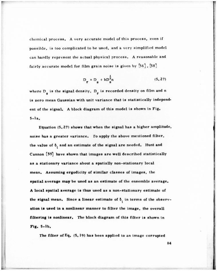
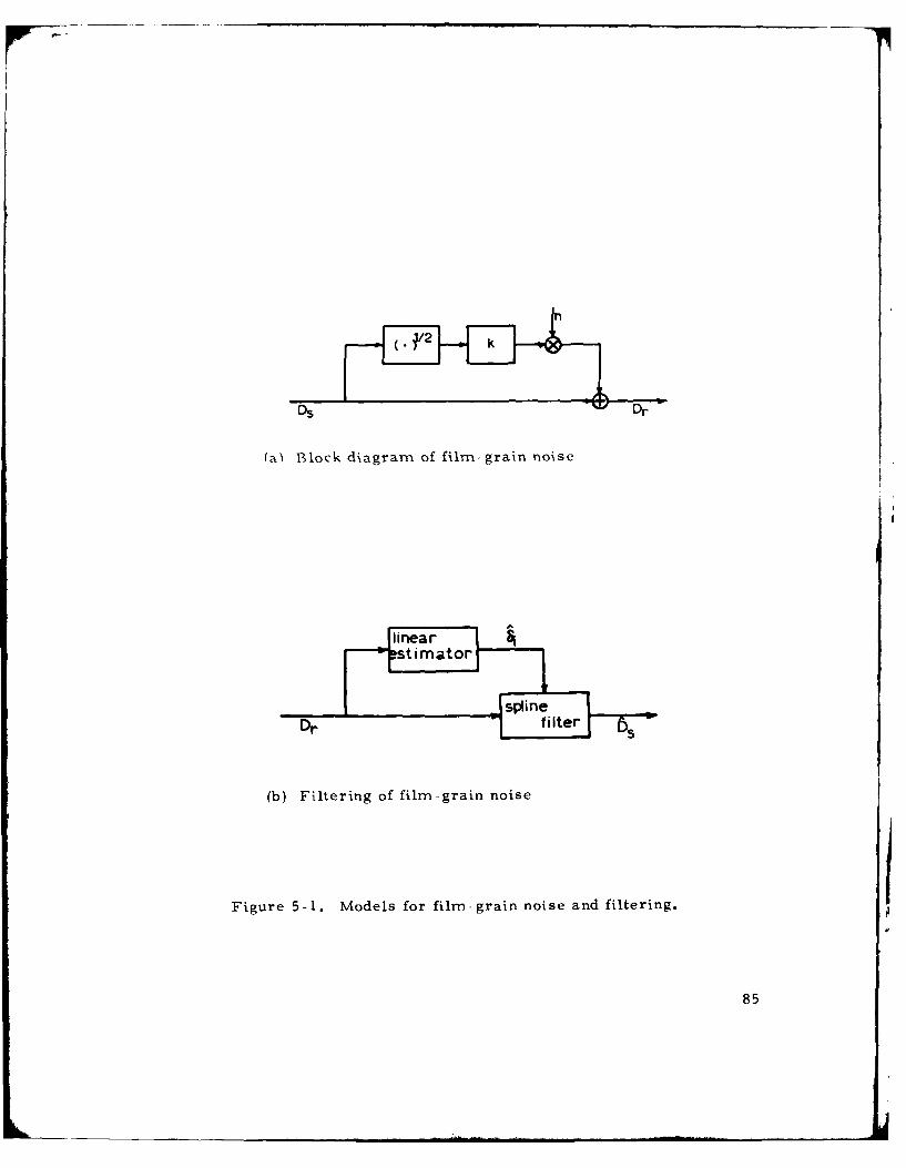
n_ (./2 k

Ds Dr

(al Block diagram of film-grain noise

=sllt i m at o

Dr -I f i ter s

(b) Filtering of film-grain noise

Figure 5-1. Models for film-grain noise and filtering.

85

a) Original

(b) Noisy, signal-depenident )Fil re.cd

Figure 5 2. Filtering of signal dependi n! noisNy imlag.~tS

4.4

44

0

0

$4'-44

00

f4

87

by signal-dependent noise modeled by Eq. (5. 27) when k = 2. Figure

5-2a is the original image, Fig. 5-2b is the noisy image and Fig.

5-2c is the filtered result. Figure 5-3a is a plot of the brightness

cross-section of Fig. 5-2a, and the subsequent plots are brightness

cross-sections of noisy and filtered images. The filter has reduced

the mean square error by a factor of ten.

5.4 Restoration of Noisy Blurred Images

A noisy blurred image can be expressed in the form

H f +n (5.28)

for a discrete model, where f and & are samples of the object and

image functions given by (5.20a) and (5.20b), respectively. The

following fidelity criteria for image restoration may then be

formulated as minimization ofXN2

j (f"(x))2 dx (5.29)

x 1

among all twice differentiable function feC 2 such that

l1 D '(H f-F)l!r S 5. 30)

where D is defined by Eq. (5.20c). This minimization criteria is

similar to what was defined for unblurred noisy images with a slight

modification. If H = I, the condition (5. 30) reduces to (5. 13). Using

the same procedure as before, the objective function

8

XN_ _(f"(x))dx + pE 1-1(H -g)12 + z - S] (5. 31)

xl

must be minimized with respect to f. Assuming the function f to be

composed of piecewise polynomials given by (5. 17), the equations

rc Qt a (5.32)t -2

Q c = pHID (-Ha) (5.33)

are obtained, where

tIc2 , cV .. . CN it (5.34)

-1

[ala 2 .... aN (5. 35)

and Q and T are previously defined. In order to satisfy condition(5. 18), cI and c are assumed Lo be zero. Since r is a positive

n

definite matrix

c = r-Qa (5. 36)

and substituting (5. 36) in (5. 33) yields1 F I ta t -2

Q' Qa = pHD (g-Ha). (5.37)

From (5. 17), it is clear that a = f therefore

-t 2 -1I t-I t -

S (HtDH +XQ r Q)-HD y (5.38)-1

where X = p . SettingH= I leads to the estimate of Eq. (5. Z6).

Comparison of this restoration filter to the Wiener filter given by

-1(5.7) shows the similarity of these two filters with.Cf replaced by q

Il tXQ T-Qt. In order to obtain the filter numerically, it is necessary

t - 2 -lI tto invert the matrix T as well as H D H + XQT-Q t . Matrix T is a

positive-definite tridiagonal matrix and efficient techniques exist for

the computation of its inverse [57] . Since H is a large matrix for

ordinary size images, and also H is not of full column rank for non-

zero background pictures, the matrix HtD 2H + XR r-IQt may be

ill-conditioned or singular and thus pseudo-inversion is used instead

of exact inversion. In section 5. 6 the experimental results of this

filter are presented.

5. 5 The Fffect of Fidelity Criteria on High Frequency Suppression

In Chapter 4, describing the restoration of noiseless images, a

fidelity criteria based on the minimization of the L 2 -norm of the

function was defined which led to the filter given by (4. 19) and

pseudoinversion. In this chapter, the fidelity criterion is based on

the minimization of L2-norm of the second derivative of the function,

leading to spline filtering and restoration. In this section, the effects

of different criteria on the frequency content of the restored image

are discussed.

The objective function for both cases has the one common term

X (f (k)(x)) dx (5. 39)

where X is a weighting factor. If k = 0, the derived filter is given by

(4.19) or by pseudo-inversion, and k = 2 leads to spline restoration.

(10

Minimization of the objective function implies the reduction of term

(5. 30) in addition to the other terms. Faking the Fourier transform of

this term and applying Parseval's theorem, it is equivalent to

Xf [(2r u) kF(u)] du (5.40)

where u is the spatial frequency and F(u) is the Fourier transform of

fx). As (5.40) shows, the amplitude F(u) at spatial frequency u is

weighted by a factor (2rru) k and then squared and integrated. rhere-

fore, as k increases, the weighting factor of high frequency amplitude

increases too. rhus, reducing (5.40) with larger k implies the

suppression of the higher frequencies more than the lower frequencies.

When k = 0, the amplitudes of all the frequencies are equally weighted.

In most image restoration problems with white noise, the original

object is a relatively low frequency signal, and noise has a flat power

spectral density. When the noise power is zero or very low, there is

no need to suppress the high frequency content of the image. More-

over, preserving the higher frequencies preserves the fine details of

the image, and thus, k = 0 is a good choice for noiseless images.

Conversely, for noisy images, where most of the high frequency

content of the image belongs to the noise, k = 2 is a good choice.

Generally, as k increases, the filtered signal is more smooth and

correlated with less higher frequency content.

91

L. .. .....

5. 6 Experimental Results

In this section the experimental results of restoration of nisv

blurred images by spline functions are presented. Figure 5- 4 a

illustrates a scene of original size 128 : 128 pixels enlarged to

256 x 256 by cubic spline interpolation for display purposc's. Figure

5-4b represents the image following motion degradation with a point-

spread function of length 7 pixels and the addition of zero mean

Gaussian noise with standard deviation 1. rhe observed image has a

nonzero background, and thus the system is underdetermined. For

restoration, the smoothing parameter X of the filter (5. 38) is set to

01 and . 001, and the SVD algorithm is employed to compute the

t - 2 -1I tpseudo-inverse of the matrix H D H + XQ T Q t .

Figure 5-5 shows the behavior of singular values for different

values of X. When X is small, it only affects the smaller singular

values (right side portion of the curves) which correspond to high

frequency eigenvectors, while for large X, the smoothing term

Q r-Q t completely dominates the deblurring term HtD 2 H and its

singular values. The effect of X extends from the left side portion of

the curves to the right portion as X increases. For the computation

of the pseudoinverse a judici-us threshold c must be selected for the

cutoff of singular values. Figures 5-4c and 5-4d show the restored

image for X = .01, P= .005, and for X= .001, e = .001, respectively.

As X and e decrease, the restored image becomes sharper with

92

0

fill I D.C-

94

more details, but at the same time the amplitude of unwanted high

frequency components increases. For large X anc e, the restored

image is smoother and more correlated. Thus, by choosing these

two parameters as well as the local smoothing window 6, one can

control the tradeoff between smoothing and resolution locally and

globally. It is obvious that the quality of the restored image is

highly dependent on the proper selection of these parameters.

I

95

Chapter 6

CONCLUSIONS AND SUGGIP'S FIONS FOpR

FUR PHER RESEARCH

Phis dissertation has presented a thuoretical and experimental

analysis of image restoration in the spline domain. Representing

object, image and point-spread functions by splines has led to a

more accurate and realistic model. Ihe interesting properties of

spline functions, particularly B-splines, have been used in image

modeling and restoration.

Fhe linear integral equation that describes the image formation

has been discretized for processing by a digital computer. Various

methods such as pulse approximation, Newton-Cotes and monospline

quadrature formulae are discussed and compared with each other.

rhe first two methods are special and extreme cases of the third

one. It is shown that the monospline quadrature formulae of degree 3

produces less error overall than the other two methods, although the

best choice of degree for the monospline is dependent on the variation

of the integrand and sampling interval. For the class of rapidly

varying functions, a smaller m is advised, but for the class of

slowly varying functions, large values of m give better results.

rhese results are true for both undersampled and oversampled

functions.

96

B-splines have been used for interpolation and approximation of

object and image functions. B-splines havy- some advantages over the

sine and cosine basis functions of the Fourier domain. First, they

are strictly positive and thus they are a better representation of image

intensity. Second, the shape of these functions is fixed except for a

shift of location. This property results in circulant matrices which

are easy to handle numerically. Third, their local basis properties

results in banded matrices. Fourth, their convolutional property

represents the convolution integral of space-invariant degradations.

It has been shown that using B-splines and exploiting the convoluti3nal

property for restoration of an analytically blurred image results in a

more accurate reconstruction of the original object. Since the blurred

image is generally smoother than the object, a higher degree B-spline

represents it better than the one representing the object. rhe degree

of B-spline must be selected according to the frequency content (or

variation) of the approximated function.

Fhe minimum norm criteria leading to the pseudo-inversion has

been used for the restoration of space-variant degradations, over-

determined models and underdetermined models. A numerical

technique called singular-value-decomposition is used for computa-

tion of the pseudo-inverse. Due to the singularity of the system,

ill-conditioning or roundoff error, a judicious threshold for the

nonzero singular values must be made. A sudden decrease in their97

i

values and the machine precision are the determining factors. Ihe

strikingly good results for the restoration of astigmatism which is

strongly space-variant show the validity of the objective criteria and

the capability of the numerical technique.

A constrained least squares criteria based on the minimization

of the second derivative and local statistics of the noise has been

defined and the optimal filter, which produces a cubic spline function

as the estimate, has been derived. this filter is applicable to both

space-variant and space-invariant degradations. rhe parameters of

the filter determine the local smoothing window and overall extent of

smoothing and thus the tradeoff between resolution and smoothing is

controllable both locally and globally. Fhese properties have made

the spline filter capable of restoring images with signal-dependent or

multiplicative noise. rhis filter has been successfully applied for

filtering images degraded by film-grain noise which is modeled as

signal-dependent or multiplicative noise. Since a local spatial

average has been used as a nonstationary estimate of the signal mean

and local smoothing factor, the overall filtering is nonlinear. fhe

filter has been also applied to images degraded by motion blur and

noise. Fhe results show that as the smoothing parameter decreases,

the restored image becomes sharper with more details, but at the

same time the amplitude of unwanted high frequency components

increases. For large smoothing parameters, the restored images

98

become more correlated. Finally, the effect of fidelity criteria on

high frequency components of the restored image has been analyzed.

If the noise power is zero or almost zero, the fidelity criteria based

on the minimization of the function is advised, but for noisy images,

the fidelity criteria with respect to the minimization of the second

derivative of the function gives better results.

Irhe research pursued in this dissertation may be extended in

several directions. A more detailed study of monospline quadrature

formulae, particularly free nodes, would be of considerable interest.

Fhe number of nodes and their locations have substantial effect on

quadrature error and accuracy of the discrete model. rhis study can

be extended with respect to the behavior and local properties of the

integrand. In approximating the image function by splines, variable

sampling may be studied for optimal knot placement and error re-

duction. A discussion of the problem as well as some algorithms

may be found in references [60] , [61].

A more detailed experimental study of the spline filter is

particularly useful in determining the parameters of the filter

according to the local properties of the image and noise statistics.

rhe filter can be applied to non-uniform sampling with minor

modification of the filter matrices [Appendix A] . rhus the

sampling intervals may be determined with respect to local behavior

of the observed image and then the modified filter can be used.

99

Recursive computational techniques are of special interest in

real-time processing of the images. A version of the filter may be

developed for restoring images when the stream of data comes from

a scanner or transmitter. Another possibility would be an exploration

of the iterative method for solution of the filter. Such a method has

been developed for computation of the pseudoinverse [621, [63]

Since the matrices of the spline filter are banded circulant or

Foeplitz, very efficient numerical techniques, particularly for

space-invariant degradations, may be used.

As mentioned earlier, spline functions have many desirable

approximating and interpolating characteristics that can be used in

various areas of digital image processing. So far, some attention

has been given to potential applications of spline functions in image

restoration and enlargement [45] , [64] . Although this is just

beginning work in utilizing the properties of spline functions in image

restoration, the successful results indicate that further fruitful

research can be performed in this field. Spline functions may be used

in other areas of digital image processing such as image coding and

reconstruction of images from their projections.

100

APPENDIX A

DI'RIVA[ION OF [tIP SMOOCFIING SPLINI: FI[LFER

Condition (5. 18) implies c I = cN = 0. Substituting (5.17) in

(5. 1 6 a), (5.16b), (5. 1 6 c) and (5.16d) yiLlds

2 3a i+) a.i + b h.i + c.h + d.h. i 1. N-I (A-i)

b b. + 2c.h. + 3d.h. i 1,...,N-I (A-2)i+1 I I I 1 i

c = c. + 3d.h. i 1... N-I (A-3)

3(d. di 1 ) V62 1,..., N-1 (A-4)

where h i = xi+.-I, i = 1,...,N-1 and g = g(xi). Obtaining d. from

(A-3), b. from (A-i) and substituting these two values in (A-2) and1

(A-4) gives

c= (C i+ 1 -c)/(3h) (A-5)

bt (ai+ -a.)/h. - cih. - dh (A-6)

ii i+ Ii I.I IhI

1 a 1__,f 1 1 h i 4-1 + h 4h i ,/

h i+Z h., ai+ h. + 3 ci+2+ Z 3 i+li+l 1 3 1

h.I . (A-7)

-c + (,~+-c. +jc. p(a.-)6 (A -8)h."+ i+ 2 Z h~ h i i+l i = °a-gi *

101

I-,•

Using vt-,tor space notation, Vqs. (A-7) and (A-8) can be writtvin as

1' c a (A- 9)-2

=Q p (g-a) (A-10)

where C= fc 2 .... CN -1 a = a r is a positive de-

finite tridiagonal matrix of order N-2 with elements

h 4h hi+

3 3

and Q is a N X (N-2) tridiagonal matrix with elements

1 1 1 1

q, hhi+l hi j+2 ~lii 1

Premultiplying both sides of Eq. (A-10) by QtD2

QtD Qc = pQ-t pQta (A-11)

and substituting Qta from (A-9) into (A-11) gives

(QDQ + p')c = pQ. (A-12)

Since Qt D 2Q + pr is positive definite, c amy be obtained as

_ = p(QtD2S + pT)-1 Qg. (A-14)

From (A-10), a is derived as

-1 2Qa = Q-p D c (A-14)

Substituting (A-13) in (A-14) gives

102

d)- -Q(QtD Q p.l- Q .E

Since f = a, the filtLr is given as in Eq. (5. 19).

103

APPENDIX B

MATRIX IDEN FI fY

Lemma: For any nonsingular matrices B and C, the following matrix

identity

-1 -1 t-1 1At(C +A B A = C-CA(ACA+B) AC

-1 -1At -1 -1is valid for any matrix A if (C +A B A and (A C A+B) exist.

Proof: Assuming an auxiliary matrix D of the form

-1 B-1AtD = C +AB A (B-l)

-1and premultiplying both sides of Eq. (B-l) by D gives

-I -1 -1 -I tI = D C +D AB A t (B-21

Postmultiplying (B-2) by C, the equation

-I -l -1 tc B3C =D -1+ D- AB -1A tC (B -3)

is obtained, and this is rewritten as

D- -D A B Ac . (B-4)

Postmultiplying (B-3) by A gives

-l -l -1 t CCA = D A+D AB ACA

-1 -l t C=D A(I + B ACA)

=D AB(B +ACA). (B-5)

104

Since the inverse of B + At C A exists, D A B is obtained as

D IAB = CA(B+A C A) ( B-6)

and this can be substituted in (B-4) to give

D- C C A(B + ArC A) A tC (B-7)

or from (B-i)

--1 -1 -1 t(C +A B A) = C-CA(B+ACA) AC. (B-8)

Q. E.D.

105

REFERENCES

I. H. C. Andrews, "Digital Image Restoration: A Survey," IEEEComputer, Vol. 7, No. 5, pp. 36-45, May 1974.

2. H. C. Andrews and C. L. Patterson, "Outer Product Expansions

and rheir Uses in Digital Image Processing, " Aerospace Corp.,El Segundo, Calif., Rep. ArR-74 (8139)-2, Jan. 1974.

3. A. Marechal, P. Croce and K. Dietzel, "Amelioration duContraste de Dtails des Images Photographiques Par Filtrage

des Frequences Spatiales," Opt. Acta Vol. 5, pp. 256-262, 1958.

4. M. M. Sondhi, "Image Restoration: rhe Removal of Spatially

Invariant Degradations, " Proceedings of the IEEE, Vol. 60, No.

7, July 1972.

5. J. Fsujiuchi, "Corrections of Optical Images by Compensation of

Aberrations and by Spatial Frequency Filtering, " in Progress in

Optics, Vol. 2, Wiley, New York, pp. 131-180, 1963.

6. J. L. Harris, Sr., "Image Evaluation and Restoration," J. Opt.

Soc. Amer., Vol. 56, pp. 569-574, May 1974.

7. B. L. McGlamery. "Restoration of rurbulence-DegradedImages," J. Opt. Soc. Amer., Vol. 57, pp. 293-297, March1967.

8. P. F. MuellerandG. 0. Reynolds, "Image Restoration by

Removal of R-indom Media Degradations," J. Opt. Soc. Amer.,

Vol. 57, pp. 1338-1344, November 1967.

9. C. W. Helstrom, "Image Restoration by the Method of Least

Squares," J. Opt. Soc. Amer., Vol. 57, pp. 207-303, March

1967.

10. D. Slepian, "Linear Least-Squares Filtering of Distorted IMages,"

J. Opt. Soc. Amer., Vol. 57, pp. 918-922, Tuly 1967.

11. W. K. Pratt, "Generalized Wiener Filter Computation

Techniques," IEEE rrans. Computers, pp. 636-641, july1972.

106

12. A. Habibi, "Fast Suboptimal Wiener Filtering of Markov

Processes," University of Southern California, Image ProcessingInstitute Technical Report USCIPI Report 530, Los Angeles, CA

90007, pp. 75-80, March 1974.

13. F. Davarian, "Fast Computational Techniques for Pseudoinverse

and Wiener Image Restoration, " Ph. D. Dissertation, Departmentof Electrical Engineering, University of Southern California,Image Processing Institute, rechnical Report USCIPI Report610, Los Angeles, CA, 90007, August, 1975.

14. B. R. Hunt, "rhe Application of Constrained Least Squares

Estimation to Image Restoration by Digital Computer, " IEEETransaction on Computers, Vol. C-ZZ, No. 9, pp. 805-812,

September 1973.

15. E. R. Cole, "The Removal of Unknown Image Blurs by

Homomorphic Filtering," Ph. D. Dissertation, Department ofElectrical Engineering, University of Utah, Salt Lake City, Utah,

84112, June 1973.

16. N. Mascarenhas, "Digital Image Restoration Under a Regression

Model - rhe Unconstrained, Linear Equality and InequalityConstraint Approaches," Ph.D. Dissertation, Department of

Electrical Engineering, University of Southern California, ImageProcessing Institute Technical Report, USCIPI 520, Los Angeles,

CA, 90007, January 1974.

17. H. C. Andrews, "Positive Digital Image Restoration Techniques;

A Survey, " Aerospace Corp., El Segundo, Calif. , Rep. ArR-73(8138)-Z, Feb. 1973.

18. A. V. Oppenheim, R. W. Schaefer, and r. G. Stockham,"Nonlinear Filtering of Multiplied and Convolved Signals, "

Proc. IEEE, Vol. 56, pp. 1264-1291, Aug. 1968.

19. r. G. Stockham, T. M. Cannon, R. B. Ingebretsen, "Blind

Deconvolution Through Digital Signal Processing," Proc. IEEE,Vol. 63, No. 4, pp. 678-69Z, April 1975.

20. B. R. Hunt, "Digital Signal Processing," Proc. IEEE, Vol. 63,

No. 4, pp. 693-708, April 1975.

107

21. L. J. Cutrona, "Recent Development in Coherent Opticalrechniques," in Optical and Electro-Optical InformationProcessing, J. r. rippett etal., Eds., M. I. F. Press, Cam-bridge, Mass. 1965.

22. A. A. Sawchuk, "Space-Variant Image Restoration by Coordinaterransformation, " J. Opt. Soc. Amer., Vol. 64, No. 2, pp.138-144, Feb. 1974.

23. J. W. Goodman, Introduction to Fourier Optics, McGraw-Hill,New York, 1968.

24. A. A. Sawchuk, and M. J. Peyrovian, "Restoration of Astigma-tism and Curvature of Field, " J. Opt. Soc. Amer., Vol. 65,No. 4, pp. 712-715, June 1975.

25. A. A. Sawchuk, "Space-Variant Image Motion Degradation andRestoration," Proceedings of IEEE, Vol. 60, No. 7, July 1972.

26. G. M. Robbins and r. S. Huang, "Inverse Filtering for LinearShift-Variant Imaging Systems, " Proceedings of IEEE, vol. 60,No. 7, July 1972.

27. r. S. Huang, "Some Notes on Film Grain Noise," in WoodsHoles Summer Study Rep. on Restoration of AtmosphericallyDegraded Images, Vol. 2, Alexandria, VA., DefenseDocumentation Center, pp. 105-109, July 1966.

28. F. Naderi and A. A. Sawchuk, "Nonlinear Detection andEstimation of Images Degraded by Film-Grain Noise," Proc.Opt. Soc. Amer., ropical Meeting on Image Processing,Asilornar, Calif., Feb. 24-26, 1976, pp. 17-24.

29. A. G. rescher and H. C. Andrews, "Data Compression andEnhancement of Sampled Images," Applied Optics, Vol. 13, No. 1,January, 1974.

30. r. N. Cornsweet, Visual Perception, Academic Press, New York,1970.

31. I. J. Schoenberg, "Monospline and Quadrature Formulae,"['heory and Application of Spline Functions, I. N. E. Greville,pp. 157-207, Academic Press, New York and London, 1969.

108

12. A. Ralston, A First Course in Numerical Analysis, M(;raw-till, New York, 1)65.

3 1. I'. N. V. Greville, Theory and Application of Spline Functions,

Academic Press, New York, IQ69.

14. J. C. Ilolladay, "Smoothest Curve Approximation,' Math. rables

Aids Comput. 11, pp. 233-243, 1q57.

35. C. de Boor, "Best Approximation Properties of Spline Functionsof Odd Degree," J. Math. Mech. 12, pp. 747-749, 19(3.

36. I. 1. Schoenberg, "Spline Functions and the Problems ofGraduation," Proc. Nat. Acad. Sci. U.S.A. 52, pp. 947-950,1064.

37. L. L. Schumaker, "Some Algorithms for the Computation ofInterpolating and Approximating Spline Functions," 1Theory andApplication of Spline Functions, r. N. E. Greville, pp. 87-102,Academic Press, New York, 1969.

38. H1. B. Curry and I. J. Schoenberg, "On Polya Frequency Func-tions IV. Fhe Fundamental Spline Functions and Their Limits,

J. Analyse Math. 17, pp. 71-107, 1966.

39. M. H. Schultz, Spline Analysis, Prentice-Hall, Englewood Cliffs,

N.J., 1973.

40. I. J. Schoenberg, "On Monospline of Least Square Deviation andBest Quadrature Formulae," SIAM J. Numer Anal. Ser. B-2,

pp. 144-170, 1965.

41. I. J. Schoenberg, "On Monospline of Least Square Deviation andBest Quadrature Formulae II, " SIAM J. Numer Anal. 3, pp.321-328, 1966.

42. F. Davarian and M. J. Peyrovian, "Quadrature Formulae Appli-cation in Image Restoration," University of Southern California,Image Processing Institute Technical Report, USCIPI Report560, Los Angeles, CA, 90007, pp. 60-67, March 1975.

43. M. J. Peyrovian and A. A. Sawchuk, "Image Restoration bySmoothing Spline Functions, " University of Southern California,Image Processing Institute technical Report, USCIPI Report620, pp. 86-92, September 1975.

109

44. A. Albert, K. gression and the Moore-Penrose Pseudoinv-crsc,

Acadn'ic tPress, New York, 1972.

45. 11. S. Ilou, 'Least Squares Image Restoration Using SplineInterpolation, '' Ph. 1). Dissertation, Department of Flectrical

Engineering, University of Southern California, Image Process-ing Institute, Technical Report USCIPI Report 650, pp. 86(-4 2,September 1975.

46. G. H. Golub and C. Reinsch, "Singular Value Decomposition andLeast Squares Solutions," Numer. Math., Vol. 14, pp. 403-420,1970.

47. M. Born and F. Wolf, Principles of Optics, Fourth Edition,Pergamon Press, London, 1070.

48. G. M. Robbins, Mass. Inst. Fech Res. Lab Electronics Quart.Prog. Report, No. 93, pp. 243-251, 1969.

4. IV. K. Pratt, Digital Image Processing, to be published.

50. A. Papoulis, Probability, Random Variables, and StochasticProcesses, McGraw-Hill, New York, 1965.

51. P. Liebelt, An Introduction to Optimal Estimation, Addison-Wesley, Menlo Park, Calif, 1969.

52. B. R. Hunt and H. C. Andrews, "Comparison of Different Filter

Structures for Image Restoration, " Proc. 6th Annual Hawaii

Int. Conf. on System Sciences, Jan. 1973.

53. C. H. Reinsch, "Smoothing by Spline Functions," Numer. Math.,

Vol. 10, pp. 177-183, 1967.

54. C. H. Reinsch, "Smoothing by Spline Functions, II" Numer.

Math., Vol. 16, pp. 451-454, 1971.

55. R. S. Martin and J. H. Wilkinson, "Symmetric Decomposition ofPositive Definite Banded Matrices, " Numer. Math., vol. 7,pp. 355, 1965.

56. J. F. Walkup and R. C. Choens, "Image Processing in Signal-

Dependent Noise," Optical Engineering, Vol. 13, pp. 258-266,1974.

110

57. E. L. Allgower, "Fxact Inverses of Certain Band Matrices,

Numer. Math., Vol. 21, pp. 279-284, 1973.

58. F. Naderi, "Estimation and Detection of Images Degraded by

Film-Grain Noise," Ph.D. Dissertation, Department of

Electrical Engineering, University of Southern California,

Image Processing Institute, Los Angeles, CA, 90007, August,

1976.

59. B. R. Hunt and r. M. Cannon, "Nonstationary Assumptions for

Gaussian Models of Images, " Fo appear in IEEE Trans. Systems,

Man and Cybernetics.

60. C. de Boor and J. R. Rice, "Least Square Cubic Spline Approxi-

mation I: Fixed Knots," Computer Science Department, Purdue

University, Rep. CSD TR 20, Lafayette, Indiana, 47907, 1968.

61. , "Least Square Cubic Spline Approximation II:

Variable Knots," Computer Science Department, Purdue Uni-

versity, Rep. CDS rR 21, Lafayette, Indiana, 47907, 1968.

62. r. S. Huang, D. S. Baker, and S. P. Berger, "Iterative ImageRestoration," Applied Optics, Vol. 14, No. 5, pp. 1165-1168,May 1975.

63. r. S. Huang, "Restoring Images with Shift-Varying Degradations,'

Proc. Opt. Soc. Amer. roptical Meeting on Image Processing,Asilomar, California, pp. 149-151, Feb. 24-26, 1976.

64. H. C. Andrews, and C. L. Patterson, "Digital Interpolation of

Discrete Images," IEEE Trans. Computer, pp. 196-202,

February, 1976.

1l1