nanogrid topology, control and interactions in a microgrid
TRANSCRIPT

Nanogrid topology, controland interactions in amicrogrid structure
by
Daniel Burmester
A thesissubmitted to the Victoria University of Wellington
in fulfilment of therequirements for the degree of
Doctor of Philosophyin Computer Science.
Victoria University of Wellington2018


Abstract
Distributed generation, in the form of small-scale photovoltaic installa-tions, have the potential to reduce carbon emissions created by, and alle-viate issues associated with, centralised power generation. However, themajor obstacle preventing the widespread integration of small-scale pho-tovoltaic installations, at a residential level, is intermittency. This thesisaddresses intermittency at a household/small community level, throughthe use of “nanogrids”. To date, ambiguity has surrounded the nanogridas a power structure, which is resolved in this thesis through the deriva-tion of concise nanogrid definition. The nanogrid, a power distributionsystem for a single house/small building, is then used to implement de-mand side management within a household. This is achieved through theuse of a hybrid central control topology, with a centralised coordinatingcontroller and decentralised control nodes that have the ability to senseand modulate power flow. The maximum power point tracker is used toobserve the available photovoltaic power, and thermostatically controlledloads present in the household are manipulated to increase the correlationbetween power production and consumption. An algorithm is presentedwhich considers the expected power consumption of the thermostaticallycontrolled loads over a 24 hour period, to create a hierarchical ratio. Thisratio determines the percentage of available photovoltaic power each loadreceives, ensuring the loads that are expected to consume the most powerare serviced with the largest ratio of photovoltaic power. The control sys-tem is simulated with a variety of household consumption curves (alteredfor summer/winter conditions), and a week of realistic solar irradiancedata for both summer and winter. In each simulated scenario, a compari-

son was made between controlled and uncontrolled households to ascer-tain the extent grid power consumed by a household could be reduced,in turn reducing the effect of intermittency. It was found that the sys-tem had the ability to reduce the grid power consumed by as much as61.86%, with an average reduction of 44.28%. This thesis then exploresthe concept of interconnecting a small community of nanogrids to form amicrogrid. While each nanogrid within the network has the ability to op-erate independently, a network control strategy is created to observe thepossibility of further reducing grid power consumed by the community.The strategy considers the photovoltaic power production and thermo-statically controlled loads operating within the network. A ratio of thenetwork’s photovoltaic power is distributed to the thermostatically con-trolled loads, based on their expected consumption over a 24 hour period(highest consumption receives largest ratio of power). This was simulatedwith a range of household cluster sizes, with varied consumption patterns,for a week with summer/winter solar irradiance. The tests show that,compared to an uncontrolled nanogrid network, the combined control canreduce grid power consumed by as much as 55%, while a 7% decrease isseen when comparing the combined control to the individually controllednanogrid networks. When compared to an uncontrolled individual housescenario, the combined control interconnected nanogrids can reduce thepower purchase from the grid by as much as 61%.

Papers Published From ThisThesis
1. Daniel Burmester, Ramesh Rayudu, Winston KG Seah. ”Use of Maxi-mum Power Point Tracking Signal for Instantaneous Management ofThermostatically Controlled Loads in a DC Nanogrid”, IEEE Trans-actions on Smart Grid (in print), DOI 10.1109/TSG.2017.2704116, 2017
2. Daniel Burmester, Ramesh Rayudu, Winston KG Seah, Daniel Akinyele.”A Review of Nanogrid Topologies and Technologies”, Renewableand Sustainable Energy Reviews, vol 67, p 760-775, Elsevier, 2017
3. Daniel Burmester, Ramesh Rayudu, Winston KG Seah. ”A Com-bined Control Strategy for Load Management within an Intercon-nected Nanogrid Network”, IEEE Innovative Smart Grid Technologies-Asia (ISGT-Asia), 2017
4. Daniel Burmester, Ramesh Rayudu, Winston KG Seah. ”Instanta-neous Control of a DC Water Heater for a PV System”, IEEE Inter-national Conference on Power System Technology (POWERCON),2016
5. Daniel Burmester, Ramesh Rayudu, Winston KG Seah. ”Instanta-neous Nanogrid Control Using Maximum Power Point Tracking Sig-nal”, IEEE Innovative Smart Grid Technologies-Asia (ISGT-Asia), 2016
iii

iv
6. Daniel Burmester, Ramesh Rayudu, Winston KG Seah. ”DistributedGeneration Nanogrid Load Control System”, IEEE PES Asia-PacificPower and Energy Engineering Conference (APPEEC), 2015
7. Daniel Burmester, Ramesh Rayudu, Winston KG Seah. ”A Compari-son Between Temperature and Current Sensing in Photovoltaic Max-imum Power Point Tracking”, IEEE Eighteenth National Power Sys-tems Conference (NPSC), 2014
8. Daniel Burmester, Ramesh Rayudu, Edwin Massold. ”Setup of aNanogrid for Teaching Purposes”, 21st Electronics New Zealand Con-ference (ENZCON), 2014
9. Daniel Burmester, Ramesh Rayudu, Edwin Massold. ”Proposed NanogridLoad Control Algorithm”, 21st Electronics New Zealand Conference(ENZCON), 2014

Acknowledgments
I would like to thank my family and friends for their support which hasenabled me to pursue my research and complete this thesis. I would alsolike to thank my supervisors, Dr Ramesh Rayudu and Prof Winston Seahfor their guidance and wisdom, the SPRES group for their advice and in-sightful discussions, and the wider ECS community. Lastly, I would like tothank the Victoria doctoral scholarship and Victoria doctoral submissionscholarship for the financial support which has allowed me to devote timeto my research.
v

vi

Contents
1 Introduction 1
1.1 Motivation . . . . . . . . . . . . . . . . . . . . . . . . . . . . . 2
1.1.1 Gaps in the Research . . . . . . . . . . . . . . . . . . . 3
1.2 Research Statement and Objectives . . . . . . . . . . . . . . . 4
1.3 Major Research Contributions . . . . . . . . . . . . . . . . . . 6
1.4 Research Strategy . . . . . . . . . . . . . . . . . . . . . . . . . 8
2 Literature Review 11
2.1 Nanogrids . . . . . . . . . . . . . . . . . . . . . . . . . . . . . 12
2.1.1 Nanogrid Control . . . . . . . . . . . . . . . . . . . . . 12
2.1.2 Nanogrid Hardware . . . . . . . . . . . . . . . . . . . 15
2.2 Thermostatically controlled loads . . . . . . . . . . . . . . . . 22
2.3 Interconnected nanogrid network . . . . . . . . . . . . . . . . 24
2.4 Chapter Summary . . . . . . . . . . . . . . . . . . . . . . . . . 28
3 Nanogrid Topology and Definition 31
3.1 Definition and Background of Nanogrid . . . . . . . . . . . . 32
3.1.1 Nanogrid - A Definition . . . . . . . . . . . . . . . . . 33
3.1.2 Types of Nanogrid Technology . . . . . . . . . . . . . 35
3.1.3 Nanogrid Control Topologies . . . . . . . . . . . . . . 43
3.2 Chapter Summary . . . . . . . . . . . . . . . . . . . . . . . . . 49
vii

viii CONTENTS
4 Nanogrid Control System 514.1 Nanogrid System . . . . . . . . . . . . . . . . . . . . . . . . . 51
4.1.1 Maximum Power Point Tracking . . . . . . . . . . . . 524.1.2 Central and Node Controllers . . . . . . . . . . . . . . 59
4.2 Thermostatically Controlled Loads . . . . . . . . . . . . . . . 674.2.1 Water and Space Heating . . . . . . . . . . . . . . . . 674.2.2 Refrigerator . . . . . . . . . . . . . . . . . . . . . . . . 78
4.3 Simulation, Results and Discussion . . . . . . . . . . . . . . . 824.4 Chapter Summary . . . . . . . . . . . . . . . . . . . . . . . . . 91
5 Interconnected Nanogrid Network 935.1 Nanogrid Network Scenarios . . . . . . . . . . . . . . . . . . 95
5.1.1 Uncontrolled Nanogrid Network . . . . . . . . . . . . 955.1.2 Individually Controlled Nanogrid Network . . . . . 985.1.3 Combined Control Nanogrid Network . . . . . . . . 100
5.2 Simulation, Results and Discussion . . . . . . . . . . . . . . . 1075.2.1 The Effect of Varied PV Capacities . . . . . . . . . . . 110
5.3 Chapter Summary . . . . . . . . . . . . . . . . . . . . . . . . . 115
6 Conclusions and Future Work 1176.1 Future Work . . . . . . . . . . . . . . . . . . . . . . . . . . . . 123
A Load Characteristics 157

Chapter 1
Introduction
Existing power infrastructures are currently facing a number of adversitieswhich, inherently, they are ill-equipped to resolve. These problems stempartly from the use of long distance transmission lines delivering powerfrom large central generators to consumers [1, 2]. This method of powerdistribution leads to major line losses, which reduces the grid’s efficiency[3]. It also makes the grid susceptible to costly power outages causedby environmental (e.g. heavy rain or wind) and non-environmental (e.g.equipment failure due to age) events [4,5]. These large central power gen-erators are often fossil fuel based solutions, contributing to the 30.8 billiontons of carbon dioxide released into the atmosphere each year [6]. Anothermajor issue is the estimated 1.2 billion people globally, who do not haveaccess to electricity [7]. A majority of these people live in rural or isolatedcommunities, to where extending the grid is often considered uneconom-ical [8, 9].
For social, environmental and financial reasons these inadequacies needto be addressed and one solution under research is distributed generation(DG) [10,11]. DG looks to remedy the issues inherent in the current powersystem, by producing power close to the point of use [12]. This reduces theneed for long distance transmission, increasing efficiency and creating arobust system (reducing outages) [13]. The power capacity of DG is much
1

2 CHAPTER 1. INTRODUCTION
smaller than a central power generator, making it a versatile power solu-tion [14]. So much so that it can enable a typical consumer of power to alsoproduce power from their residential or commercial property. This makesDG a structure capable of meeting power requirements for consumers liv-ing in rural or isolated communities [15]. And as distributed generation isoften, but not limited to renewable, carbon neutral energy (e.g. wind andsolar), it also has the ability to reduce global carbon emissions [16].
1.1 Motivation
Distributed generation, particularly renewable energy (RE), has two ma-jor disadvantages preventing its widespread integration into residential/commercial properties [17]. The first is the intermittent nature of its poweroutput [18]. Take for example photovoltaic modules, of which the outputpower fluctuates with the energy produced by the sun, causing variationsin magnitude frequently over the course of a day [19]. As most electric-ity consumers expect power instantaneously, such intermittency can deterconsumers from investing in RE [20]. The second is the financial capitalrequired to install RE sources and the lengthy payback time before seeinga financial return [21].
Globally, feed-in tariffs are offered by a number of countries to offsetthe set up cost, incentivising the installation of renewable energy sources(such as photovoltaic (PV) modules) [22]. However, there are a large num-ber of countries, for instance New Zealand (NZ), where no feed-in tariff isoffered. In NZ, power is purchased by the customer for approximately28c/kWh and around 10c/kWh is received for power sold back to thegrid [23, 24]. This decreases the viability of PV installations, discourag-ing the uptake of carbon neutral power sources at a time when stringentgreenhouse gas targets are being set by the government. In these instances,an alternative must be sought to incentivise PV systems, making them aneconomically viable option.

1.1. MOTIVATION 3
The research undertaken for this thesis looks to address these issuesfrom a technical perspective. This entails using a controlled power struc-ture to increase the correlation between power production and consump-tion, exploring the potential to reduce the effects of intermittency and in-crease the financial viability of PV. The controlled power structure selectedfor this role is the nanogrid.
1.1.1 Gaps in the Research
Chapter 2 presents a comprehensive summary of the literature surround-ing the nanogrid field of research. From this analysis a number of gapswere identified which give context to this research and further motivatethe thesis. These are as follows:
• Nanogrid definition: While there are a number of characteristics sug-gested within the nanogrid literature to differentiate the nanogridfrom other power structures, the definition itself is vague and varies.
• Thermostatically controlled loads: Undertaking a variety of roles withinthe literature, to offer customers financial benefits, thermostaticallycontrolled loads typically require external influence such as pricingschemes or utility company control signals. The research fails tooffer independent control strategies, utilising multiple thermostat-ically controlled loads, to incentivise the uptake of PV.
• Maximum power point tracking control signal: Used traditionally formaximising the output of PV modules, the maximum power pointtracking signal is not used within the literature to implement loadcontrol strategies.
• Interconnected nanogrid network: Relatively new in the nanogrid lit-erature is the concept of connecting multiple nanogrids to create a

4 CHAPTER 1. INTRODUCTION
larger power entity (e.g microgrid). Control strategies, specificallystrategies that consider all the nanogrids within the larger entity toform a cohesive control structure, are not yet presented within theliterature.
The goal of addressing the disadvantages associated with householdPV installations, combined with the gaps within the nanogrid literature,have led to the formation of the research statement and research objectivesfor this thesis.
1.2 Research Statement and Objectives
Small-scale renewable energy sources have the potential to both reducecarbon emissions and reduce the pressures on, and inefficiencies of, cen-tralised energy grids. But, despite these benefits, the intermittent natureand financial cost of renewable energy presents a daunting challenge forindividuals and small community users when adopting small-scale re-newable energy sources. This study investigates the use of control withina nanogrid to reduce the effects of intermittency, making small-scale re-newable energy more accessible to individuals and small scale communityusers. The control strategy will then be expanded to facilitate interactionsbetween multiple nanogrids, forming a microgrid, to evaluate the poten-tial to further reduce the effects of intermittency.
To achieve this research statement, the following research objectiveshave been set:
1. The issue with the current literature is that it leaves the definition ofa nanogrid structure ambiguous, suggesting various characteristicsand/or bounds to differentiate the nanogrid as its own power struc-ture. The distinction between a nanogrid and micro-/macrogrid mustbe made for the following reasons:

1.2. RESEARCH STATEMENT AND OBJECTIVES 5
• Nanogrids play a different role to micro-/macrogrids in the powerhierarchy. For example, by connecting multiple nanogrids a mi-crogrid can be formed. This introduces an alternative approachto the traditional microgrid, which can only be discussed giventhe distinction between nanogrids and microgrids.
• The potential markets for nanogrids are different to that of micro-/macrogrids. A nanogrid allows a power structure to be ob-tained at a relatively low cost compared to micro-/macrogrids.This then shifts the interest from large/multiple investors, tohome/small business owners.
• As the nanogrid structure is confined to a single home, the tech-nical objectives, hardware and software often vary from that ofa micro-/macrogrid. By refining the subject area, it clarifies thefield of research.
To ensure this distinction can be made, a concise definition of a nanogridstructure must be derived from the various characteristics suggestedwithin the current literature.
2. A nanogrid control strategy that will increase the correlation betweenpower consumption and PV production, reducing the negative ef-fects of solar intermittency, will be developed. The strategy shouldhelp to reduce power purchased and sold by the consumer, from/tothe power grid, helping to incentivise small scale PV systems. Toavoid additional cost, an alternative to traditional purpose-specificstorage methods (eg battery banks) should be sought. The systemshould be simulated under a variety of load/solar irradiance con-ditions comparing the grid consumption of the controlled nanogridwith the uncontrolled to ascertain the reduction in grid power con-sumed by the nanogrid.
3. A control strategy that will facilitate an interconnected nanogrid net-

6 CHAPTER 1. INTRODUCTION
work will be developed. This will allow the sharing of power withina cluster of houses, taking advantage of the diverse power consump-tion patterns the households will present. The nanogrid control strat-egy should be extended to consider the combined consumption andproduction of a cluster of houses to further reduce the effects of inter-mittency. When simulated, a comparison between the uncontrolledcluster, individually controlled cluster and combined control clustershould be made to quantify the success of the solution. A success-ful solution should see the combined control reduce the grid powerconsumed by the cluster of houses when compared to the other twoscenarios.
1.3 Major Research Contributions
The implementation of these research objectives will deliver the followingmajor research contributions:
1. This thesis presents a rigorous analysis of the general nanogrid defi-nitions given within the literature, discussing their merits and weak-nesses from which a concise definition of a nanogrid structure is de-rived. The traditional supply side management control structuresare presented and extended to include demand side management.A new control structure which improves the hybrid central controlstrategy is also presented.
Part of this contribution has been published in: Daniel Burmester,Ramesh Rayudu, Winston KG Seah, Daniel Akinyele. ”A review ofnanogrid topologies and technologies”, Renewable and SustainableEnergy Reviews, vol 67, p 760-775, Elsevier, 2017
2. This thesis develops a novel nanogrid control scheme that makesuse of thermostatically controlled loads to address intermittency ofphotovoltaic (PV) modules, negating the need for traditional storage

1.3. MAJOR RESEARCH CONTRIBUTIONS 7
and enabling the user to reduce grid power consumed. This strategyshifts away from direct or indirect control signals received from theutilities and introduces the concept of using a maximum power pointtracking signal to instantaneously shift electricity consumption, dy-namically matching local PV production. Simulated under a varietyof load and solar irradiance conditions, the nanogrid control schemeshows the ability to reduce grid power consumed by 44%.
Part of this contribution has been published in: Daniel Burmester,Ramesh Rayudu, Winston KG Seah. ”Use of Maximum Power PointTracking Signal for Instantaneous Management of ThermostaticallyControlled Loads in a DC Nanogrid”, IEEE Transactions on SmartGrid (Accepted for publishing), DOI 10.1109/TSG.2017.2704116, 2017
3. This thesis presents a control scheme that facilitates the interconnec-tion of multiple nanogrids. This scheme extends the capabilities ofthe single nanogrid control to dynamically match the consumptionand production of a cluster of interconnected households. This con-trol scheme further reduces the effect of intermittency, taking ad-vantage of diversity of consumption within a cluster of houses. Acomparison of grid power consumed by the cluster of houses is pre-sented, considering uncontrolled, individually controlled and thecombined control scenarios. The simulated tests show that, com-pared to an uncontrolled nanogrid network, the combined controlcan reduce power purchased by as much as 55%, while a 7% de-crease is seen when comparing the combined control with the in-dividually controlled nangrid networks. When compared to an un-controlled individual house scenario, the combined control intercon-nected nanogrids can reduce the grid power consumed by as muchas 61%.

8 CHAPTER 1. INTRODUCTION
1.4 Research Strategy
This thesis investigates the topology, control and interconnection of nanogridsto motivate the uptake of PV at a household level. In order to achieve thegoals set out, the following research strategy was developed:
• To situate the research within the nanogrid field and gain knowledgeof the area of research, it was important to perform an initial litera-ture review. From this, the successful control approaches could beidentified to help guide the research direction, and gaps in the con-trol theory could be identified, delivering avenues for improvement.As nanogrid research is frequently progressing, it was also impor-tant to regularly update the literature review, staying informed ofthe state of the art.
• Once this knowledge base was established and gaps in research iden-tified, initial ideas for a new solution were mind mapped. Thesewere refined into a pseudo algorithm which address the mains pointsof action for the solution. A mathematical representation of the pseudoalgorithm was developed, before it was coded.
• In order to evaluate the impact of the solution, it was decided a simu-lated comparative case study would be implemented. The compara-tive study would observe the grid power consumed by a household,with and without the proposed solution. The success of the out-come would be quantified by the magnitude in which the grid powerconsumed by the household was reduced. To ensure the modelledhousehold load curve did not present biased results, ten differenthousehold loadlines were established, which were simulated withsolar irradiance data for a week in summer and winter.
• Once the simulated test scenarios were established, an iterative pro-cess was established which involved analysis of results, reflection

1.4. RESEARCH STRATEGY 9
and progression. The analysis looked successful the solution wasand where there was room for improvement. Then, during the reflec-tion, strategies were developed for addressing the shortcomings ofthe solution, of which the most effective was selected. This was thenadded to the solution and the progressed model was re-simulatedand evaluated.

10 CHAPTER 1. INTRODUCTION

Chapter 2
Literature Review
In order to situate the research presented in this thesis and affirm its nov-elty, the research areas surrounding the thesis have been reviewed andpresented in this chapter.
The contributions of this thesis include work in the nanogrid controlarea, so the major trends and contributions in the nanogrid control litera-ture are outlined and discussed. While nanogrid hardware is not a focusof this thesis, it closely relates to the control and is a major research areawithin the nanogrid literature. For this reason, the hardware and its func-tion within the nanogrid is presented as well as the novel converter typesoffered by the nanogrid literature.
In this thesis, the nanogrid control would not be possible without theuse of thermostatically controlled loads. In fact, the manner in which theyare used within the system itself adds novelty to the thesis. For this rea-son, the literature concentrating on thermostatically controlled loads is re-viewed giving an overview of the definition, motivations and implemen-tations of these flexible loads.
Lastly, interconnected nanogrid network research presented in the lit-erature is reviewed with the advantages, future directions, and the state ofthe art analysed.
11

12 CHAPTER 2. LITERATURE REVIEW
2.1 Nanogrids
Nanogrids first made an appearance within the literature in 2004 [25], in-creasing in popularity from 2010 as shown with the plot of a keywordsearch (Elsevier and IEEE database) in figure 2.1. The literature can be splitroughly into the following groups: Nanogrid control; Nanogrid hardware;Interconnected nanogrid networks; Works summarising the nanogrid con-cept including future developments. The majority of the literature fallsinto the first two categories (control and hardware), with a small numberof conceptual papers and the relatively recent addition of the intercon-nected nanogrid network topic.
An in-depth discussion of the nanogrid topology and definition is pre-sented in chapter 3, but for clarity and context within the literature review,a nanogrid is defined as:
“ a power distribution system for a single house/small building, with the abil-ity to connect or disconnect from other power entities via a gateway. It consists oflocal power production powering local loads, with the option of utilising energystorage and/or a control system.”
2.1.1 Nanogrid Control
Nanogrid control can be divided into two categories; supply side manage-ment (SSM) and demand side management (DSM). Supply side manage-ment focuses on controlling the nanogrid’s supplies and energy storage(such as PV, small scale wind turbines, battery banks, etc) to ensure thedemand (load) is met and/or the state of charge (battery banks) is opti-mised. This is an important aspect of nanogrid control as often multiplesources exist and their integration needs to be balanced in such a way thata specific source can be selected to supply the nanogrid (eg with a gridtied PV system, it is favourable to supply the loads with the PV first, be-fore supplying the unmet load with the grid).
The most popular form of SSM within the nanogrid literature is droop

2.1. NANOGRIDS 13
year2004 2005 2006 2007 2008 2009 2010 2011 2012 2013 2014 2015 2016
Num
ber o
f pap
ers
publ
ishe
d
0
5
10
15
20
25
30
35
40
45
50Number of Papers Related to Nanogrids
Figure 2.1: Number of nanogrid papers published since its realisation.
control [25–34]. In DC nanogrids the bus voltage is monitored, as the loadincreases, the bus voltage “droops” (while in AC, frequency droop canbe used) with certain voltage levels engaging the appropriate supply (eg380V-375V photovoltaic supply, 375V-370V battery bank supply added,370V-365V grid supply added).
There are also alternative solutions, for example using nodes to routepower as suggested in [35]. The goal of the system is to ensure all loadsare supplied with the appropriate power while ensuring the generators arenot overloaded. This is achieved with multi-port nodes that can select theappropriate path between a generator and load via communication and a“request/offer” routing algorithm.
Maximum power point tracking is often used in nanogrids when pho-

14 CHAPTER 2. LITERATURE REVIEW
tovoltaic modules are used as a supply. Typically these are in series withthe photovoltaic modules, adjusting the impedance seen by the modulesin order to ensure the maximum power is extracted from them. In [36]however, SSM is implemented within the nanogrid to create a maximumpower point tracker that operates in parallel with the photovoltaic mod-ules. It adjusts the power from an additional power source (eg grid) tomeet the difference between the load’s requirement and the maximumpower point of the photovoltaic modules, which reduces losses in the sys-tem.
Demand side management on the other hand, manipulates the load tomeet the characteristics of the supply, which is the focus of the researchpresented in this thesis. This can be achieved in a number of ways, with avariety of different primary motivations.
Load shedding is a DSM technique where the loads are switched off toachieve a desired control goal. Authors of [26] and [37] use load sheddingto reduce peak load demand and to prevent overloading of the DC bus.Much like the droop control discussed above, DC bus signalling is used(droop control) in this case to switch off designated loads when certainvoltage levels are reached.
Load scheduling adds a level of flexibility to DSM. Rather than switch-ing off loads, the control strategy calculates an appropriate time for theload to operate. The control signals, techniques and indeed motivationsfor implementing this control strategy varies throughout the literature.In [38] and [39], the control signal is obtained for the utilities (grid powersupplier) in the form of real time pricing. This takes advantage of dynamicpower pricing, shifting consumption to times when a low power price isoffered (off peak price). [38] defines this as an optimisation problem, inthe form of an “optimal stopping problem”, with the goal of minimisingcost or maximising profit. In [39], a rule-based method is used to moveor reduce the load when the price of power is high. Storage is also con-

2.1. NANOGRIDS 15
sidered in this system, either charging or discharging the battery bank toanticipate future increases in the power price.
Another objective of load scheduling is flattening peak demand as sug-gested in [40]. The motivation behind this system is to reduce the differ-ence between peaks and troughs of a household’s power usage. This inturn creates a flatter demand reducing the grids operational costs, includ-ing transmission, generation, and fuel costs. This system uses “Least SlackFirst” policy, inspired by the “Earliest Deadline First” algorithm to shiftthermostatically controlled loads based on control signals received fromthe utility companies (real-time electricity prices and demand-responsesignals from the grid).
2.1.2 Nanogrid Hardware
There are a variety of technologies used with nanogrids, but the subjectthat dominates the nanogrid literature is converter topologies. Convertersare responsible, within the nanogrid, for manipulating voltages to meetthe requirements of a specific task. This is typically (but not limited to)interfacing the nanogrid’s sources with the system’s bus and the nationalgrid, along with interfacing the nanogrid’s loads with the bus as shown inFig. 2.2 [41]. The common categories of converters used in nanogrids are,DC to DC, DC to AC and AC to DC [42].
DC to DC converters accept a DC voltage at the input and output amodified DC voltage. The amplitude of the converter’s output voltage canbe smaller or larger than the input voltage. To achieve this change in am-plitude, the converters use reactive components (capacitors and inductors)and switching components such as diodes, metal-oxide-semiconductor field-effect transistors (MOSFETs) and insulated-gate bipolar transistors (IG-BTs) [43, 44]. By rapidly switching the converter between states, usingpulse width modulation (PWM), the necessary output voltage can be at-tained. Moreover, by measuring the output (or input) voltage (or current)

16 CHAPTER 2. LITERATURE REVIEW
Renewable Source
Non-Renewable Source
Renewable Source
Source Converter
Source Converter
Source Converter
Load 1
Load ...
Load n
Source Converter
Source Converter
Source Converter
Storage Converter
Storage
Bus
Figure 2.2: Hardware structure of a nanogrid
of the converter, the PWM can be altered to ensure the output voltageremains stable even when the input voltage varies. This property is essen-tial when implementing nanogrid control strategies such as droop control.The most commonly used DC to DC converter topologies are buck styleconverters (output voltage is always less than the input), boost style con-verters (output voltage is always greater than the input) and buckbooststyle converters (output voltage can be either greater or less than the in-put).
It is easy to see then, how these converters may be used within a DCnanogrid. Take for example Fig. 2.2, here the source converters would takethe varying/low DC input voltage and boost the output to the required380 V for the DC bus. At the other end of the chain the load converter willbuck (reduce) the bus voltage (380 V) to a level the loads can use (12 V, 24V or 48 V).
There are other tasks the converters can perform within the nanogrid,such as maximum power point tracking (MPPT) of a renewable source orcharge controlling a battery bank. The goal of MPPT is to address the non-linearities presented to a system by a renewable source (primarily photo-

2.1. NANOGRIDS 17
voltaics but can also apply to wind turbines) [45]. A converter being usedfor MPPT is controlled with the PWM, according to an MPPT algorithm,to present an optimum impedance to renewable energy source. This is toensure the source is always operating at its maximum power output [46].Charge controllers make use of converters to regulate the speed of charg-ing and ensure battery banks are not overcharged, which lengthens the lifeof a battery bank [47].
DC to AC converters accept a DC voltage at the input and output anAC voltage. This procedure is also implemented with reactive compo-nents, switching components and PWM. DC to AC converters often havea DC to DC converter front end to ensure the DC input is of the rightamplitude for the AC conversion. The DC to AC converter has similarcharacteristics to the AC to DC converter, which accepts an AC voltage asan input and outputs a DC voltage. In fact it is not rare to see bidirectionalconverters of this nature. As the name would suggest, these are convert-ers that can work as an AC to DC converter, and in reverse, a DC to ACconverter. This is ideal for grid tied DC nanogrids which will in some cir-cumstances feed the grid AC power, and in others receive power from theAC grid which will need to be converted to DC for the nanogrid.
The research undertaken within the nanogrid literature is focused onincreasing the efficiency of the converters used within the nanogrid. Italso looks to improve power quality for the loads that require high powerquality, reduce the physical size of the nanogrid system and increase theease of controllability within the nanogrid. These goals are achieved byresearching multiple input/ output converters, switching variations, gal-vanic isolation and alternative topologies [48]. Table 2.1 outlines somenovel converter hardware contributions within the research on nanogrids.

18 CHAPTER 2. LITERATURE REVIEW
Table 2.1: Novel converter hardware contributions from nanogrid research
Converter technology Type of con-verter
Hardware novelty
Dual-active-bridge basedbidirectional micro-inverter [49]
BidirectionalDC to AC
This converter makes use of Lithium-Ion Ultra-Capacitors (LICs) forshort term storage in a synchronousboost converter, which improves thenanogrid’s power quality by reduc-ing the dP/dt factor of photovoltaicmodules and increases fuel economyof the diesel generators.
Multi-port power con-verter architecture [50]
DC to DC The proposed converter topology re-places the control switch of a con-ventional boost converter with a full-bridge network consisting of fourswitches creating both an isolated andnon-isolated output for devices thatrequire galvanic isolation and thosethat do not.
Boost-derived hybrid con-verter [51]
DC to DC andDC to AC
The control switch of a conventionalboost converter is replaced with abidirectional single-phase bridge net-work. This provides an AC out-put and DC output simultaneouslywhich is a benefit when operating ananogrid with both AC and DC loads.

2.1. NANOGRIDS 19
Multi-input single-inductor converter [52]
DC to DC The conventional topology of a multi-input, single-output DC-DC con-verter uses multiple inductors to filterthe output voltage. The multi-inputsingle-inductor converter replaces themultiple inductors with a single in-ductor reducing the cost of the con-verter.
Dual-input interleavedbuck/boost converter [53]
DC to DC Proposed is a dual-input isolated dc-dc converter which interleaves a buckand boost converter circuit. This con-verter also makes use of galvanic iso-lation on the output, making the sys-tem ideal for use in hybrid renewableenergy systems with an energy stor-age system present.
Single-stage multistringphotovoltaic inverter [54]
DC to AC This inverter is a grid-tied multistringconverter with a high-frequency AClink, soft-switching operation, andhigh-frequency galvanic isolation.This means an arbitrary numberof photovoltaic modules can beconnected and the converter cangain maximum power from each.This converter provides high effi-ciency, high power density and highreliability.
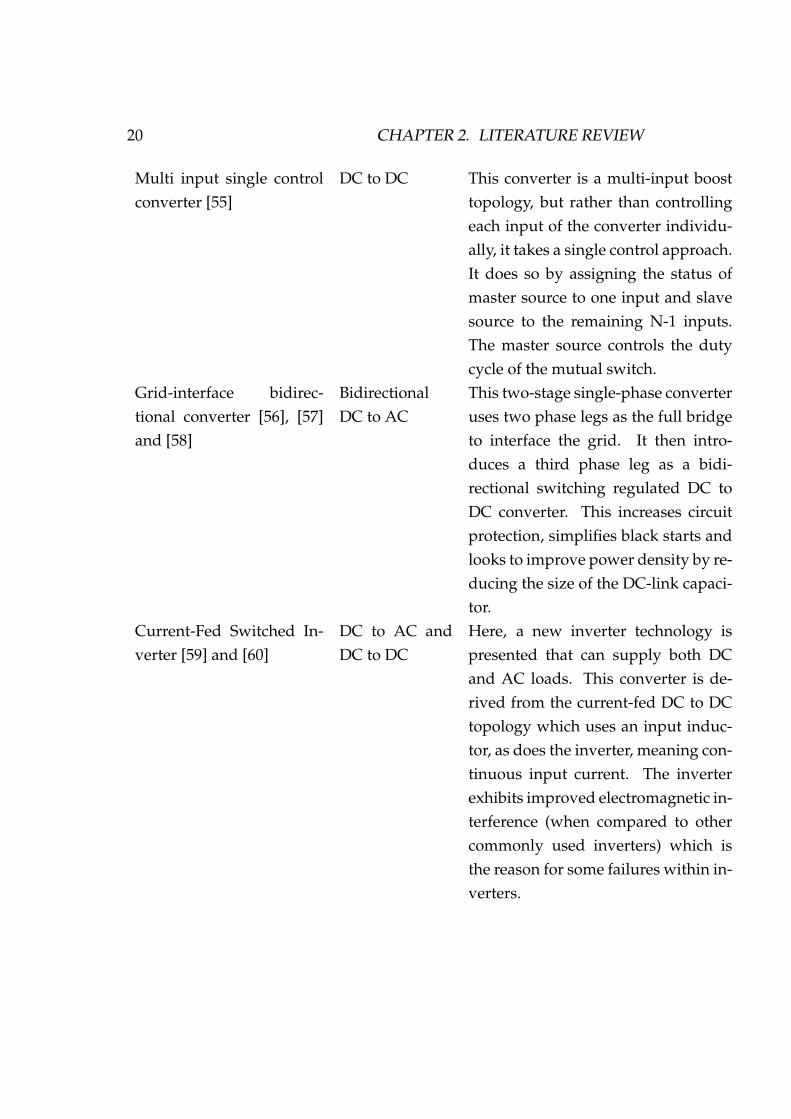
20 CHAPTER 2. LITERATURE REVIEW
Multi input single controlconverter [55]
DC to DC This converter is a multi-input boosttopology, but rather than controllingeach input of the converter individu-ally, it takes a single control approach.It does so by assigning the status ofmaster source to one input and slavesource to the remaining N-1 inputs.The master source controls the dutycycle of the mutual switch.
Grid-interface bidirec-tional converter [56], [57]and [58]
BidirectionalDC to AC
This two-stage single-phase converteruses two phase legs as the full bridgeto interface the grid. It then intro-duces a third phase leg as a bidi-rectional switching regulated DC toDC converter. This increases circuitprotection, simplifies black starts andlooks to improve power density by re-ducing the size of the DC-link capaci-tor.
Current-Fed Switched In-verter [59] and [60]
DC to AC andDC to DC
Here, a new inverter technology ispresented that can supply both DCand AC loads. This converter is de-rived from the current-fed DC to DCtopology which uses an input induc-tor, as does the inverter, meaning con-tinuous input current. The inverterexhibits improved electromagnetic in-terference (when compared to othercommonly used inverters) which isthe reason for some failures within in-verters.

2.1. NANOGRIDS 21
Isolated bidirectionalACDC converter [43]
BidirectionalAC to DC
This converter suggests the use ofmultiple switching technologies in-cluding insulated-gate bipolar tran-sistors (IGBTs) without an antiparal-lel diode, MOSFETs, and silicon car-bide (SiC) diodes. With this comesa frequency detection method usingan advanced filter compensator, a fastquad-cycle detector, and a finite im-pulse response (FIR) filter.
Switched boost in-verter [61] and [41]
DC to AC andDC to DC
This inverter is based on the inverseWatkins-Johnson topology. However,it implements a DC output on thediode leg of the DC to DC convertersection. It also makes use of shootthrough current, meaning this con-verter can either buck or boost its out-put voltage.
Cuk-derived hybrid con-verter [48]
DC to AC andDC to DC
To create both AC and DC powerfrom a Cuk converter, the controlswitch is replaced with a single phasevoltage source inverter bridge net-work. Three modes of operation arethen defined by utilising the bridgeswitches allowing the Cuk-derivedhybrid converter to achieve the re-quired goal of creating AC and DCpower.
22 CHAPTER 2. LITERATURE REVIEW
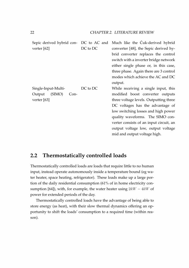
Sepic derived hybrid con-verter [62]
DC to AC andDC to DC
Much like the Cuk-derived hybridconverter [48], the Sepic derived hy-brid converter replaces the controlswitch with a inverter bridge networkeither single phase or, in this case,three phase. Again there are 3 controlmodes which achieve the AC and DCoutput.
Single-Input-Multi-Output (SIMO) Con-verter [63]
DC to DC While receiving a single input, thismodified boost converter outputsthree voltage levels. Outputting threeDC voltages has the advantage oflow switching losses and high powerquality waveforms. The SIMO con-verter consists of an input circuit, anoutput voltage low, output voltagemid and output voltage high.
2.2 Thermostatically controlled loads
Thermostatically controlled loads are loads that require little to no humaninput, instead operate autonomously inside a temperature bound (eg wa-ter heater, space heating, refrigerator). These loads make up a large por-tion of the daily residential consumption (61% of in home electricity con-sumption [64]), with, for example, the water heater using 2kW − 4kW ofpower for extended periods of the day.
Thermostatically controlled loads have the advantage of being able tostore energy (as heat), with their slow thermal dynamics offering an op-portunity to shift the loads’ consumption to a required time (within rea-son).

2.2. THERMOSTATICALLY CONTROLLED LOADS 23
The majority of the literature surrounding the use of thermostaticallycontrolled loads concentrates on implementing control based on signalsreceived from grid operators (utility companies) [65–104]. There are anumber of motivations for the utility companies to pursue this control,eg; grid frequency control, grid voltage control, help to mitigate the neg-ative effects of increased renewable energy penetration in the grid. Thecontrol signals come in two forms, direct and indirect control.
Direct control systems receive instruction directly from the utility com-panies which allow them to turn on/off thermostatically controlled loadswhen necessary. While this technique has fast feedback, it can create alevel of discomfort for the end user. The user comfort, for example havinghot water when required, is a topic of much discussion within the directcontrol scheme literature.
Indirect control on the other hand is implemented by the user withincentives supplied by the utility companies to ensure cooperation. Thethermostatically controlled load algorithms in this area of research con-centrate on controlling the on/off times of the loads to coincide with offpeak pricing. The motivation for the end user is a reduction in their costof power, and in turn allows the utility companies to offer off peak pricingduring times of low power use.
Thermostatically controlled loads have also been used within micro-grids to address the stabilisation of high renewable energy source pene-tration systems. This can refer to grid tie-line, smoothing power fluctua-tions, and improving power quality [105, 106]. Another strategy is to usethermostatically controlled loads to avoid large spikes in the consumptioncurve and to match the stochastic power generation of renewable energysources. This is addressed in [107], where a microgrid central load serv-ing entity is implemented to perform direct load control. The central loadserving entity can set the temperature of a building’s air conditioning unitto shift its consumption. It considers the renewable energy production to

24 CHAPTER 2. LITERATURE REVIEW
be a wind turbine, with simplified “on” or “off” output.
At a single house level, optimisation techniques (such as particle swarmoptimisation) and/or scheduling algorithms are used to shift thermostat-ically controlled loads to accommodate events such as charging of elec-tric vehicles, reduction of peak power and optimisation of energy use[108–111].
The research presented in [112] looks to increase the photovoltaic “self-consumption ratio” (photovoltaic power used in the home) through thecontrol of an electric water heater. The control system has the ability toaccess the two elements in the electric water heater separately to give itthree consumption levels (each element is a different load and the thirdis the two elements on simultaneously). The system is then optimised touse the three levels of power consumption to better utilise the local photo-voltaic power consumed.
2.3 Interconnected nanogrid network
A nanogrid is a versatile power structure, as it addresses the power re-quirements of the end user. This makes it ideal for creating a hierarchicalpower system that takes advantage of diversity within a community. Byinterconnecting nanogrids, sharing power and communication, a micro-grid can be created.
Much like a nanogrid, a microgrid is a power distribution system withthe ability to island itself from other power entities. However, a nanogrid’scapabilities are targeted at powering a single house/small building, whilea microgrid spans hospitals, university campuses and/or small communi-ties (as the case may be with interconnecting nanogrid networks).
Although the theory behind interconnected nanogrid networks, in gen-eral, is still at a high level, exploration has begun and implementation isbeing pursued.
The advantages and future research topics for nanogrid networks are

2.3. INTERCONNECTED NANOGRID NETWORK 25
outlined in [113–117], these are:
• Bidirectional power sharing is the main function of a nanogrid network.Houses/small buildings are almost guaranteed to have varied in-stantaneous power consumption curves and may also have variedpower production capabilities. The diversity of electronic devicesand consumer behaviour is responsible for the variety of consump-tion curves. This is similar with power production, where the re-newable energy source, capacity, and use of storage all play a rolein creating varied production patterns. In the case of a nanogrid net-work, the diversity works in its favour to utilise the sharing of excesspower [118]. As consumption/production peaks and troughs of in-dividual nanogrids vary within the nanogrid network, it is likely thatthe demand can be met by the various connected nanogrids. By shar-ing power within the nanogrid network, the need to purchase powerfrom an external source (national grid) is reduced. This equates to fi-nancial savings for the consumers within the network.
• Communication is an important aspect within the nanogrid networkas it lies at the heart of information sharing, which is what creates anintelligent network [119]. There are multiple layers of communica-tion within a nanogrid network and as with any information sharing,a number of technical and security based considerations. The lay-ers consist of internal nanogrid communication, which the nanogridcontroller uses to gather data and implement control strategies per-taining to single house/building level power flows. The next layeris microgrid communication which organises power offers/requestsbetween individual nanogrids and may deal with the financial as-pect of selling/buying power within the network and to the nationalgrid. The national grid level will focus on DSM/SSM at the nationallevel but would also be expected to have minimal involvement inday to day communication. This then creates a complex communi-

26 CHAPTER 2. LITERATURE REVIEW
cation network where delicate information is shared. Although thetechnical aspects of a communication network fitting a nanogrid net-work still requires research/ definition, it is not confined to noveltyas appropriate data protocols such as ModBus, TCP/IP and RS485already exist [120, 121].
• Financial benefit is a motivating factor for operating a controlled nanogridand is also an incentive for the interconnection of multiple nanogrids(nanogrid network) [114]. By adding a financial cost to power sharedwithin the nanogrid network, this motivation can be realised. Withinthe nanogrid network, a nanogrid can either be a source of power (ifexcess power is available from the nanogrid) or a load (if power is re-quired by a nanogrid). If a source, the nanogrid can sell power eitherto another connected nanogrid at a negotiated price, or to the na-tional grid at the set buyback price. As the price within the nanogridnetwork can be negotiated based on variables such as quantity ofavailable excess power and grid buyback/purchase price, the cost ofpower can be customised to benefit both the buyer and seller. Mean-ing power can be sold within the network at a price less than the gridpurchase price but greater than the buyback price.
• Withstanding power grid outages is important now our lives rely soheavily on power. The nanogrid network has the ability to island it-self from the national grid in the case of a blackout. In islanded modethe nanogrid network will be an individual power entity, servicingthe connected nanogrids. This means the production and storagepower within the nanogrid network, like a microgrid, can continueto power loads for a period of time [122]. The period of time is de-pendent on renewable energy availability (sun/wind) and storagecapacity, but if well designed the network should be able to with-stand a lengthy blackout.
• Gradual introduction is an advantage to the nanogrid network paradigm.
2.3. INTERCONNECTED NANOGRID NETWORK 27
As nanogrids operate at a single house level, it is envisioned that theintroduction of small nanogrid networks can take place over an ap-propriate length of time [118]. This negates the need for investinglarge sums of money on replacing central power plants over a shorttime period. Instead, nanogrid networks can be integrated into theexisting national grid at a manageable rate.
• Grid stability is another consideration, though not yet pursued withina nanogrid network context. It has been suggested that the nanogridnetwork has the ability to respond quickly to commands from theutility grid. This gives the nanogrid network the opportunity to par-ticipate in grid stabilisation, voltage and frequency control and real-time pricing at a national grid level.
In these early stages of interconnected nanogrid network research, pa-pers are beginning to emerge which discuss some level control. Presentedin [123] and [124], is the analysis and optimisation of power flows be-tween nanogrids (within a network). This control is focused on ensuringthe power flows between nanogrids and the state of charge of the batterybanks are optimised for DC and hybrid (DC and AC) systems. However,these papers do not pursue demand side management nor do they attemptto increase the correlation between PV production and network consump-tion.
The research presented in [125] motivates the interconnected nanogridnetwork approach to microgrids by comparing central and distributed ar-chitectures. It concludes that the distributed generation distributed stor-age architecture (nanogrid network) has a higher efficiency, lower linelosses and less voltage drops when compared to a centralised scheme. Thissolidifies the necessity of further research into the field of interconnectednanogrid networks.
A multi-objective optimisation model is presented in [126] which worksto achieve a minimised net cost of electricity for each nanogrid within the

28 CHAPTER 2. LITERATURE REVIEW
network. It uses a local buy/sell power price scheme, as well as pricesoffered by the grid to implement energy management for local produc-tion and storage. The price scheme developed encourages the sharing ofpower between nanogrids by offering a favourable price when comparedto that offered by the grid.
One research group in particular is making progress in the area of inter-connected nanogrid networks with the implementation of a testbed. In thepapers [118,120], the team present a reasonably in depth discussion on thenanogrid network they are currently installing. The proposed nanogridnetwork operates on DC power, where the network itself is not connectedto the grid, but this option is available to individual nanogrids. The sys-tem operates on the concept that power is not sold back to the grid, butinstead power is shared exclusively within the network. A power shar-ing control technique (other than non-droop) for the testbed is presentedin [127] which facilitates the sharing of power within a cluster of houses.
2.4 Chapter Summary
An in-depth analysis of the related works presented in the literature hasbeen undertaken and summarised. The topics and general conclusionsfrom the literature review are as follows:
• Nanogrid Control: The goal of control within a nanogrid, for theuser, is to increase the system’s efficiency and reduce the cost ofpower, and from a utilities perspective, gaining stability for the grid.The two main control strategies within a nanogrid are SSM and DSM,which work to control the power sources and loads respectively. Themajor SSM technique is droop control, with only a small numberof alternatives offered in the literature. DSM is varied with a num-ber of algorithms and optimisation techniques presented. However,

2.4. CHAPTER SUMMARY 29
within the literature, there are no attempts to motivate the use ofphotovoltaics utilising the maximum power point tracking signal ormodulating the voltage to thermostatically controlled loads to varythe power consumed.
• Nanogrid Hardware: Nanogrid control and hardware are closelyrelated, as the hardware within nanogrids are responsible for ma-nipulating voltages, implementing maximum power point tracking,grid connection and controlling loads. Power electronic convertersare the main focus within the literature, which has in turn offered anumber of novel converter topologies to increase efficiency and al-low the integration of AC and DC loads/sources. While hardwareis not a major focus of this thesis in terms of novelty, the nanogridpresented does rely on converters in a number of areas.
• Thermostatically Controlled Loads: Thermostatically controlled loadscan be used to implement DSM, shifting loads to address a variety ofcontrol objectives. Generally speaking, they are used in conjunctionwith control signals, directly or indirectly obtained from the utili-ties. This allows the utility company to manipulate consumptionin exchange for incentives offered to the customer. In other cases,thermostatically controlled loads can be utilised to implement inde-pendent control within a household to serve the customer directly.The control strategy outlined in this thesis uses multiple householdthermostatically controlled loads to increase the correlation betweenhousehold consumption and PV power production, which is an un-explored area within the literature.
• Interconnected Nanogrid Network: The topic of interconnected nanogridnetworks is relatively new within the literature, explored mainly ata conceptual level until recently. While a small amount of controlresearch is beginning to appear, the strategies are concentrating onpower flows and SSM, there is no DSM strategies presented. The

30 CHAPTER 2. LITERATURE REVIEW
interconnected nanogrid combined control exhibited in this thesisutilises thermostatically controlled loads to implement a cohesiveDSM control strategy for a cluster of nanogrids.

Chapter 3
Nanogrid Topology andDefinition
The majority of the available nanogrid literature focuses on the control andhardware, with a variety of algorithms and power converter topologies be-ing discussed. The idea of utilising the nanogrid’s modular nature to forma network of interconnected nanogrids is also presented within the litera-ture, though in most cases this is still at a conceptual level. The problemwith the current literature is that it leaves the definition of a nanogrid itselfreasonably ambiguous, suggesting various characteristics and/or boundsto differentiate the nanogrid as its own power structure.
In this chapter, the general definitions given within the nanogrid lit-erature are collated and their merits and weaknesses are discussed, fromwhich a concise definition of a nanogrid structure is developed. An overviewof the control topologies are then presented, discussing not only their usefor supply side management but extending it to demand side.
Part of this chapter has been published in: Daniel Burmester, RameshRayudu, Winston KG Seah, Daniel Akinyele. ”A review of nanogrid topolo-gies and technologies”, Renewable and Sustainable Energy Reviews, vol67, p 760-775, Elsevier, 2017
31

32 CHAPTER 3. NANOGRID TOPOLOGY AND DEFINITION
3.1 Definition and Background of Nanogrid
Defining a power structure is a challenging task as opinions vary and of-ten the boundaries between power structures are hazy. A good place tostart is a point of reference. As [27–29, 113, 115–117, 120, 128–130] suggest,a nanogrid is analogous to a microgrid. So we will begin by discussingthe similarities between nano- and microgrids before identifying some keycharacteristics that can be used to separate the two power structures.
At the most basic level, by all accounts, a nanogrid is a power distribu-tion system, as is true for microgrids [57, 58, 61, 116, 131–138]. Nanogridshave the capability of operating in islanded or grid connected mode whichagain is a characteristic also found when discussing microgrids [15, 28, 29,113, 116, 139–141]. Another common trait is their ability to operate as ei-ther DC, AC or hybrid power structures [27, 116, 142–148] although thenanogrid literature clearly favours DC [25, 37, 60, 61, 131, 142, 149–153].They both consist of a source, not confined to but often, renewable en-ergy [37, 116, 153–157] and some sort of load [114, 131, 154, 158–161].
When abstracting nanogrids from microgrids, one does not have tolook past their names to get an intuitive idea as to what separates them.The implication of relative size is given, but needs to be refined further tocreate a quantitative perimeter.
Terms such as low power and complexity, used in [41, 60, 113–117, 128,131, 152, 162] to characterise nanogrids, can be difficult to define. In [60]low power is defined as a few Watts to 5 kW, whereas [113,116] define it as10-100 kW. And as nanogrid research progresses, so does the complexity ofthe control strategies, optimisation techniques and structures [30,35,37,41,154]. This is not to say the statements are not valid, nanogrids are often oflower power and less complexity than microgrids. These inconsistencies,however, do permit a level of ambiguity around the definition.
In [114, 115] another definition is introduced (also referred to in pa-pers [117, 162]) which changes the structure of the nanogrid somewhat.

3.1. DEFINITION AND BACKGROUND OF NANOGRID 33
Here nanogrid is defined as a single domain for voltage, price, reliability,quality and administration, which still works with the general consensus.However, the research then suggests that the local generation is not con-sidered part of the nanogrid itself.
This characterisation of a nanogrid is interesting as it allows systemssuch as universal serial bus (USB), power over Ethernet (PoE), universalpower adaptors and a variety of other power structures which are not con-ventionally thought of as nanogrids, to be included under the nanogriddefinition. And although value can be seen in this broad generalisation ofthe structure, it tends to add confusion to the use of the term nanogrid asit was originally intended.
This leaves a simple but effective defining characteristic, given in [29,118, 120, 129, 163–165], of a nanogrid belonging to a single home or build-ing. Microgrids often span multiple homes/buildings as shown in [15,134,166–173]. And although there is nothing in the microgrid definition to sayit cannot be confined to a single home/ building, we suggest that singlehome/building microgrids should adopt the term nanogrid.
Therefore using a single house/building power distribution system todefine a nanogrid and a multiple house/build scenario for microgrids, aclear boundary is set. It allows the discussion of a power distribution sys-tem for a single home/building to take the title “nanogrid” and a multiplehome/building distribution system to fall into the “microgrid” category.
3.1.1 Nanogrid - A Definition
With the information presented above, we can establish a concise defini-tion of the nanogrid:
“A nanogrid is a power distribution system for a single house/small building,with the ability to connect or disconnect from other power entities via a gateway.It consists of local power production powering local loads, with the option of util-ising energy storage and/or a control system.”

34 CHAPTER 3. NANOGRID TOPOLOGY AND DEFINITION
Components/structure of a nanogrid
The basic structure of a nanogrid is shown in Fig. 3.1 which consists of thefollowing components:
Figure 3.1: Nanogrid block diagram
• Local power production. One of the main features of a nanogrid is itsability to increase the efficient use of residential sized distributedgeneration. These structures can support the integration of a vari-ety of renewable and/or non-renewable energy sources. The typi-cal renewable energy sources are solar and wind, whereas the non-renewable may be sources such as diesel generators or fuel cells [25,60].
• At least one local load. Local loads are electrical household applianceswhich are supplied power by local production via the nanogrid [174].Some examples are loads such as a water heater, lighting, oven, tele-vision etc.

3.1. DEFINITION AND BACKGROUND OF NANOGRID 35
• A gateway. The gateway is a bidirectional power connection betweenother nanogrids, microgrids or the national grid. Where possiblethis will include communication with other power entities, convey-ing the nanogrid’s power requirements. However, in the case ofconnecting to the national grid, communication may not be possi-ble. The gateway also has the ability to disconnect from externalpower entities, allowing the nanogrid to operate in islanded mode.The gateway allows the nanogrid to purchase power from, and sellpower to, connected power entities, increasing the financial benefitof owning distributed generation [114, 115].
• Energy storage. The energy storage is considered optional in a nanogridstructure, but is usually present as it adds stability. The energy stor-age most suited to nanogrids, due to capacity and residential loca-tion, is a battery bank.
• Nanogrid Controller. Another element which is not completely essen-tial, but usually present, is a nanogrid controller. The controller willbe discussed further in the “Nanogrid Control” chapter.
Nanogrid versus microgrid
It should be noted that while encouraging the distinction between a nano-and microgrid, the two are not necessarily mutually exclusive. The mod-ular nature of the nanogrid delivers an opportunity to connect multiplenanogrids to then form a microgrid [165]. Fig. 3.2 shows how this group-ing may be arranged.
3.1.2 Types of Nanogrid Technology
The debate between alternating current (AC) and direct current (DC) poweris not a new argument. As we know, for the national grid AC emerged the

36 CHAPTER 3. NANOGRID TOPOLOGY AND DEFINITION
Figure 3.2: Microgrid made up of multiple nanogrids
victor, mainly due to the technical limitations at the time the grid was es-tablished [175]. With increased research into the benefits of distributedgeneration, where the supply and storage is often DC, the advantages of aDC grid are still regularly discussed. This is also a subject that frequentlyarises in microgrid and nanogrid literature, the reason being an increasein efficiency when distributing DC power [61].
A basic block diagram of the DC and AC nanogrids are displayed inFigs. 3.3 and 3.4 respectively. There are similarities between the twotopologies at the source end of the power chain, these are as follows:
• DC Source. Although there are no limitations as to what type ofrenewable/non-renewable resource is used to generate power, someare more practical than others (eg hydro is not often used in nanogridsas it requires access to a body of water, which most residential or

3.1. DEFINITION AND BACKGROUND OF NANOGRID 37
Figure 3.3: Basic block diagram of DC nanogrid
Figure 3.4: Basic block diagram of AC nanogrid
commercial properties do not have). Commonly used resources aresolar (photovoltaic modules (PV)), wind (small scale wind turbines(SSWT), which do generate AC but usually output DC as the ACfrequency varies) and battery storage (which is envisioned to in-clude plug-in hybrid electric vehicles (PHEVs) in the future) [55,128]. Diesel generators and fuel cells are also mentioned within thenanogrid literature, but not as regularly as SSWT, PV and batter-ies [60, 176].
A SSWT or PV module typically output voltage which is less than50 V) [55, 128]. Table 3.1 shows the voltage range and output power(rated capacity) of a number of SSWT, as does Table 3.2 for PV units.

38 CHAPTER 3. NANOGRID TOPOLOGY AND DEFINITION
This is not a comprehensive list of available SSWT/PV technologies,merely an example of voltage outputs/rated capacities.
There are a vast multitude of batteries available for storing chargewhich can be used during times of low SSWT or PV power pro-duction [177]. These typically come in denominations of 2V whichmeans, by creating a series string of multiple batteries, most valuescan be achieved (2V, 4V... 24V, 48V). Of course the SSWT and PVmodules can also be arranged in either series, increasing voltage (five24V, 10A PVs in series would make 120V at 10A), or parallel, increas-ing current (five 24V, 10A PVs in parallel would make 24V at 50A).The number of SSWT/PV modules selected would vary dependingon the power requirements of the loads powered by the nanogrid.
Table 3.1: Small Scale Wind Turbines for use in Nanogrids.
Brand Rated capacity (W) Voltage output (VDC)Southwest Windpower Air x 400 12,24,48
Marlec Rutland 720 12,24Aerogen Aero6gen 300 12,24
Bergey Excel 1 1000 12-48Silentwind Windgenerator 420-500 12,24,48
Table 3.2: Photovoltaic modules for use in Nanogrids.
Brand Rated capacity (W) Voltage output (VDC)Canadian Solar CS6X-305M 305 36.6
Samsung LPC247SM 247 30.4Grape Solar GS-S-260 260 31.6
Renesola Virtus II 260 30.1Schutten STM5-200W 200 36.6
• Source DC-DC Converter. A DC-DC converter is a circuit that takesan input voltage and either steps it up or down depending on the

3.1. DEFINITION AND BACKGROUND OF NANOGRID 39
required output voltage. The source DC-DC converter can be usedto fulfil a number of functions:
– Multiple Source Interface. Nanogrids can have a variety of sourcesat any one time, for example a hybrid system may have a PV ar-ray, SSWT and storage supplying power to the nanogrid. Eachsource has its own operating characteristics. In order to inte-grate the various sources into the nanogrid, each requires a DC-DC converter. The converter ensures regulation of the supplyand provides protection [55].
– Bus Voltage. The Source DC-DC converter can also be used toconvert the source voltage up to a DC bus voltage level of 380V[165,178]. This 380V has become an industry-standard interme-diate dc voltage level [128]. In the case of the AC topology, thevoltage can then be rectified. The DC bus voltage has the ad-ditional advantage of simplifying the control of the nanogrid,which is discussed in the Nanogrid Control chapter [42].
– Maximum Power Point Tracking. The behaviour of the SSWT andPV is nonlinear. Under specific environmental conditions thereis only one point of operation that ensures the maximum poweroutput. This maximum power point is dynamic and by utilisingsensors to observe the behaviour of the renewable source/environmentalconditions, this point can be tracked. This is done by varyingthe duty cycle controlling the source DC-DC converter, essen-tially presenting the source with a variable load. By creating theideal load for the environmental condition, the source is forcedto operate at its maximum power point [179].
The source DC-DC converter is usually of the boost or buckboostvariety as the source voltage typically needs stepping up [60]. Theefficiency of the these converters are greater than 85% and in somecases can achieve high nineties (%) [43, 180].

40 CHAPTER 3. NANOGRID TOPOLOGY AND DEFINITION
As the DC source and load converter for both topologies are equal, atthis point the efficiencies are the same. From here, at the load end of thepower chain, the two topologies differ.
DC nanogrid
At the other end of the power chain from the DC source, is the load. Theload has a DC-DC converter to interface it with the DC bus and the gate-way requires AC power. The conversions are as follows:
• Load DC-DC Converter. This DC-DC converter is used to step downthe bus voltage to a device (load) level. For the DC nanogrid the con-version is performed by an external DC-DC converter such as a buckconverter. Like the boost converter, the buck has an efficiency greaterthan 80% (in some cases greater than 90%) [181]. The favoured volt-age levels for this stage are 24 V or 48 V which is the standard telecomvoltage [153, 163]. Most existing DC loads are designed to run eitherat 12 V, 24 V or 48V. The range of DC loads available to purchase, incomparison to AC loads, is still extremely limited [182].
• Bi-directional AC-DC converter. A bidirectional converter is neededto interface the national grid or other power entities with the localnanogrid [183, 184]. As the nanogrid functions on DC voltage andthe grid AC, as power passes between them it needs to be convertedfrom AC-DC and vice versa. The reason a bidirectional converteris required is because when the nanogrid has excess power, it willsell the additional power to the grid (DC-AC) [185]. If the load re-quirements are greater than the local production, the nanogrid willneed to purchase power from the grid (AC-DC). The efficiency of abi-directional AC-DC converter should not be less than 80% (if de-signed properly) and well designed converters can reach efficienciesin excess of 95% [43].

3.1. DEFINITION AND BACKGROUND OF NANOGRID 41
AC nanogrid
When compared to the DC nanogrid, the AC has additional conversionsthat take place to ensure the correct power is supplied to the load. Theseadditional conversions are where the AC nanogrid loses efficiency, andthese conversions take place with [186]:
• DC-AC Converter. The DC-AC converter takes the DC voltage fromthe source converter and outputs 230 V AC (or 120 V AC dependingon origin) which can be used by the majority of consumer loads soldtoday. This is also the voltage level supplied to a nanogrid from thenational grid. This means if a converter is used that can synchroniseto the grid’s frequency of 50 Hz (60 Hz depending on origin), powercan be shared easily between the power entities. With technologieslike the inverter discussed in [54], this conversion can reach efficien-cies in excess of 90%.
• Load AC-DC Converter. The AC voltage is then converted to DC,this conversion takes place in a power adaptor (also known as a wallwart) or in the device itself. For AC loads that draw less than 15 Wof power (e.g. cell phones), the DC-DC conversion is often executedby a linear power supply. The efficiency of these devices can varyfrom 20% to 75%. Loads that draw high power, implement switch-mode power conversion which is more efficient, ranging from 50%to 90% [187]. Table 3.3, with data from [182], shows the conversionefficiencies of some common household loads.
DC nanogrid/AC nanogrid comparison
There are a number of elements to consider when comparing nanogridtopologies (DC or AC), making it difficult to determine which is “supe-rior”. If efficiency is of utmost importance, the DC nanogrid has the ad-vantage [27]. For both topologies the source DC-DC converter has a sim-
42 CHAPTER 3. NANOGRID TOPOLOGY AND DEFINITION
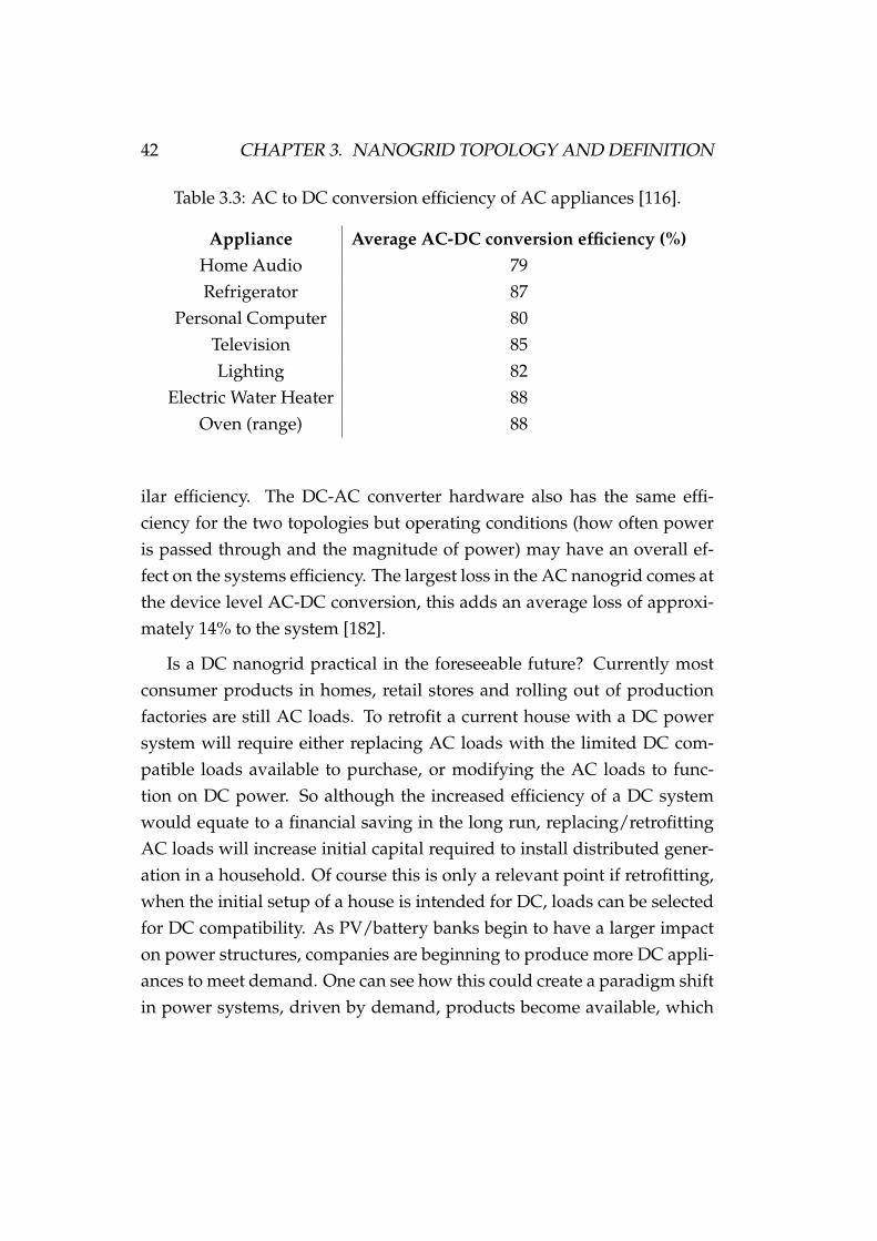
Table 3.3: AC to DC conversion efficiency of AC appliances [116].
Appliance Average AC-DC conversion efficiency (%)Home Audio 79Refrigerator 87
Personal Computer 80Television 85Lighting 82
Electric Water Heater 88Oven (range) 88
ilar efficiency. The DC-AC converter hardware also has the same effi-ciency for the two topologies but operating conditions (how often poweris passed through and the magnitude of power) may have an overall ef-fect on the systems efficiency. The largest loss in the AC nanogrid comes atthe device level AC-DC conversion, this adds an average loss of approxi-mately 14% to the system [182].
Is a DC nanogrid practical in the foreseeable future? Currently mostconsumer products in homes, retail stores and rolling out of productionfactories are still AC loads. To retrofit a current house with a DC powersystem will require either replacing AC loads with the limited DC com-patible loads available to purchase, or modifying the AC loads to func-tion on DC power. So although the increased efficiency of a DC systemwould equate to a financial saving in the long run, replacing/retrofittingAC loads will increase initial capital required to install distributed gener-ation in a household. Of course this is only a relevant point if retrofitting,when the initial setup of a house is intended for DC, loads can be selectedfor DC compatibility. As PV/battery banks begin to have a larger impacton power structures, companies are beginning to produce more DC appli-ances to meet demand. One can see how this could create a paradigm shiftin power systems, driven by demand, products become available, which
3.1. DEFINITION AND BACKGROUND OF NANOGRID 43
further drives demand for efficiency DC systems.
Within the DC nanogrid literature, protection also arises as an issue[42, 188]. The topic of this discussion focuses on protection against shortcircuit line fault, and ground fault [154]. These faults can occur at outputterminals, loads and switching devices, and severely damage a DC sys-tem [80]. These faults can be mitigated by including fault protection suchas traditional arcing-type circuit breakers, or more advanced protectionstrategies as in [154] and [189].
3.1.3 Nanogrid Control Topologies
The control of a nanogrid, implemented by the nanogrid controller, is whatgives the system the ability to coordinate multiple sources and optimisepower production and consumption. It is the “brains” of systems and ifimplemented correctly, can increase the efficient operation of the nanogrid.Within a nanogrid structure there are two categories for control, supplyside management (SSM) and demand side management (DSM). Supplyrefers to the nanogrid’s source of power, for example photovoltaic mod-ules, small scale wind turbines, grid, etc. The demand is the consump-tion of power by the household loads, for example refrigerator, television,heater, etc.
Both the supply and demand are extremely dynamic, frequently chang-ing from maximum to minimum consumption/production during a singleday [190, 191]. Unfortunately high consumption/production times rarelycoincide in an uncontrolled nanogrid system. It is for this reason that sup-ply/demand side management is an integral part of nanogrid control.
Supply side management is used to optimise the behaviour of the nanogrid’spower sources in order to best match power production to the consump-tion curve and utilise renewable energy sources. Demand side manage-ment is used to optimise the consumption curve of the nanogrid’s loads tomatch the power output of the nanogrid’s sources.

44 CHAPTER 3. NANOGRID TOPOLOGY AND DEFINITION
There are a number of control topologies that can be used to implementSSM and DSM with various levels of success. Using nanogrid controltopologies, implementation of supply side management is presented in[28, 149]. Below is an explanation of how each topology is set out for bothsupply side and demand side management with the advantages/disadvantagesof each system.
• Centralised control consists of a central controller that acts on informa-tion from sensors measuring the power production and consump-tion of the system (and in some cases other variables such as tem-perature). Fig. 3.5 shows the block diagram of the centralised con-trol topology, where the communication lines are shown in red andpower in black. As all control decisions are made from a central loca-tion, this topology has in-depth knowledge of the system dynamicsand so has the ability to implement a cohesive control strategy. Thecentralised controller measures parameters in real time, making thesystem fast when implementing control. One disadvantage to thistopology is its reliance on a high-bandwidth communications linefor collecting data from its sensors in order to implement control ina timely fashion. Another disadvantage is by centralising the controlto a single controller, the system becomes susceptible to failure. Ifa communication line or the central controller itself is damaged, thesystem will no longer have the ability to implement control.
• Decentralised control has a series of control nodes operating indepen-dently to sense the status of each local source or load. The informa-tion gathered by the node is then used to control the local source/load(as shown in Fig. 3.6). Unlike centralised control, decentralised con-trol does not require an extensive communication line, negating thisreliance. As this topology has many independent controllers, it isalso more robust than the centralised control. This makes the decen-tralised topology fast and reliable. However, as a control topology,

3.1. DEFINITION AND BACKGROUND OF NANOGRID 45
Figure 3.5: Centralised control block diagram
the decentralised scheme is limited in its usefulness. This is due tothe lack of communication between the system’s nodes. Most controlstrategies rely on the ability to force a reaction within a power sys-tem, to an event that may only be sensed by a single node. This canonly be implemented if communication between nodes exists, whichin this case, it does not [28].
• Distributed control takes the decentralised topology and adds com-munication between nodes via a communication line as in the cen-tralised control [192]. This means the distributed system adopts cer-tain characteristics of both systems. It remedies the shortcomingsof the decentralised scheme by enabling each node to communicateits power status. As each control node stores segments of an over-lying control scheme (pertaining to its own relationship to the sys-tem), the network as a whole then creates a cohesive control strat-egy. Distributed control, like decentralised control, has the advan-tage of multiple controllers reducing the likelihood of complete fail-ure within in the system. However, like the centralised control, this

46 CHAPTER 3. NANOGRID TOPOLOGY AND DEFINITION
Figure 3.6: Decentralised control block diagram
topology is dependent on communication lines. The block diagramof the distributed control is shown in Fig. 3.7.
Figure 3.7: Distributed control block diagram

3.1. DEFINITION AND BACKGROUND OF NANOGRID 47
• Hybrid Distributed control is, as the name would suggest, a hybridof the distributed control and decentralised control. As in the dis-tributed topology, the nodes can communicate creating a cohesivecontrol strategy. However, the hybrid system looks to improve onthe distributed control topology by avoiding the need to use a com-munication line, as shown in Fig. 3.8. It does so by utilising theDC bus/supply lines to communicate between nodes, as used by thepopular droop control [193]. This means the hybrid distributed con-trol does not need to rely on a communications link, increasing thereliability of the system.
Figure 3.8: Hybrid distributed control block diagram
• Hybrid Central control is taken from the centralised control schemewhich is combined with decentralised control. This creates a systemwith a central controller that communicates with decentralised con-trol nodes as shown in Fig. 3.9. The control nodes implement thesource/load level control, whereas the central controller coordinateseach node. The hybrid central control delivers a powerful and fast

48 CHAPTER 3. NANOGRID TOPOLOGY AND DEFINITION
control system with an increased resilience to failure. However, thesystem relies on communication lines which can still make it vulner-able to faults.
Figure 3.9: Hybrid central control block diagram
• There are alternatives to the traditional communication lines emerg-ing as communications play an increasingly important role withinnanogrid, microgrid and smart houses/buildings/cities. Technolo-gies such as power line communication (PLC) and DC bus signallingmake it possible to send control signals via the nanogrid’s DC/AClines. For a control scheme such as the hybrid central control, thisnegates the disadvantage of relying on a designated communicationsline. Figure 3.10 displays a topology which has the advantage of apowerful and fast control system, an increased resilience to failureand is without the vulnerability associated with the hybrid centralcontrol scheme.

3.2. CHAPTER SUMMARY 49
Load 1 Load ... Load n
DC Bus /
Source 1 Source ... Source n
ControlNode
ControlNode
ControlNode
ControlNode
ControlNode
Central Controller
ControlNode
Comms Line
Figure 3.10: Hybrid central PLC control block diagram
3.2 Chapter Summary
In this chapter, a definition for the nanogrid power structure is derived,motivated by the ambiguity of current defining attributes within the lit-erature. The various defining characteristics used within the literature todescribe the nanogrid power structure are considered, discussed and col-lated to develop a concise definition. The definition is as follows:
”A nanogrid is a power distribution system for a single house/small building,with the ability to connect or disconnect from other power entities via a gateway.It consists of local power production powering local loads, with the option of util-ising energy storage and/or a control system.”
The chapter then presents the nanogrid structure, giving a descriptionof the components used to create a nanogrid. An in-depth discussion onthe hardware similarities and variations of DC and AC power schemeswithin a nanogrid is given, before the motivating factors and considera-tions of selecting either of the power schemes is presented.
The remainder of the chapter discusses the control topologies used by

50 CHAPTER 3. NANOGRID TOPOLOGY AND DEFINITION
a nanogrid to implement demand and supply side management. Theseconsist of three main structures; centralised, decentralised and distributedcontrol, as well as the hybrid topologies derived from these.

Chapter 4
Nanogrid Control System
4.1 Nanogrid System
In this chapter a novel control strategy for a DC nanogrid is presented. Itutilises the system’s maximum power point tracking signal to implementload control taking advantage of a household’s thermostatically controlledloads. The control topology selected for this system is hybrid central con-trol with the distributed control nodes implementing real time control,while the central controller takes on a coordinating role. The block dia-gram displayed in figure 4.1 is an overview of the nanogrid system. Eachblock’s functionality is explained before the control strategy is discussedand simulated results are presented.
Part of this chapter has been published in: Daniel Burmester, RameshRayudu, Winston KG Seah. ”Use of Maximum Power Point Tracking Sig-nal for Instantaneous Management of Thermostatically Controlled Loadsin a DC Nanogrid”, IEEE Transactions on Smart Grid (Accepted for pub-lishing), DOI 10.1109/TSG.2017.2704116, 2017
51

52 CHAPTER 4. NANOGRID CONTROL SYSTEM
Constant Voltage
MPPTCentral
Controller
Converter/GatewayGrid
Standard Load 1
StandardLoad ...
StandardLoad n
DC
Bus
ThermoLoad ...
StandardNode 1
StandardNode ...
StandardNode n
DC/DCNode
Control line
Sensor system
Figure 4.1: Nanogrid block diagram
4.1.1 Maximum Power Point Tracking
The maximum power point tracker (MPPT) consists of a DC/DC converterconnected in series with a photovoltaic (PV) system and a control algo-rithm. The MPPT is used because the characteristics of a PV module de-termine that, for a particular environmental condition (specifically solarirradiance/ambient temperature), there is only one operating point wherethe maximum power can be extracted [194]. To obtain this operating point,the control algorithm monitors the appropriate variables (in most cases,PV output voltage and current) and alters the duty cycle to the DC/DCconverter to present the PV system with the required impedance [194].
In the nanogrid controller, the information acquired by the MPPT is notonly used for the traditional purpose of extracting the maximum power, itis also used for load control. The MPPT ensures the maximum PV poweroutput is not dependent on the load activities by altering the duty cy-cle to counteract load variations. This means the nanogrid control algo-rithm is presented with the maximum available PV power at any partic-

4.1. NANOGRID SYSTEM 53
ular time step, whether the system is drawing said power or not. Thisallows the load control algorithms to make instantaneous decisions basedon the available PV power.
MPPT Hardware
Traditional boost converters are regularly used in maximum power pointtracking applications with successful results [195, 196]. For this system,an interleaved boost converter was selected due to its reduced input andoutput current ripple and higher efficiency [197]. The design process out-lined in [197] was followed, with component selection outlined in equa-tions (4.1) to (4.4). An explanation of each variable within these equa-tions is given in table 4.1. DMax and DMin can also be calculated, howeverdue to the nature of MPPT, a wide range is required so DMax = 0.9 andDMin = 0.1 were assumed. The input capacitor was selected during sim-ulation, to suit the system dynamics (CIn = 100uF ). Figure 4.2 shows aschematic of the simulated interleaved boost converter.
ILAve=
0.5× IOut
1−DMax
(4.1)
IPeak = ILAve+
∆IL2
(4.2)
LMin =(VInMin
− VOn)×DMax
fs ×∆IL(4.3)
∆VOut =IOutMax
× (1−DMin)
fs × COut
+ IPeak × ESR (4.4)
MPPT Algorithm
The well defined “incremental conductance” algorithm, described in [198],was selected due to its high yield under changing conditions and its loweroscillations when compared to the perturb and observe algorithm (also
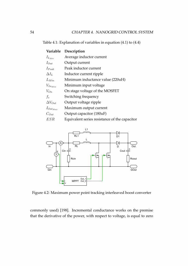
54 CHAPTER 4. NANOGRID CONTROL SYSTEM
Table 4.1: Explanation of variables in equation (4.1) to (4.4)
Variable DescriptionILAve
Average inductor currentIOut Output currentIPeak Peak inductor current∆IL Inductor current rippleLMin Minimum inductance value (220uH)VInMin
Minimum input voltageVOn On stage voltage of the MOSFETfs Switching frequency∆VOut Output voltage rippleIOutMax
Maximum output currentCOut Output capacitor (180uF)ESR Equivalent series resistance of the capacitor
Figure 4.2: Maximum power point tracking interleaved boost converter
commonly used) [198]. Incremental conductance works on the premisethat the derivative of the power, with respect to voltage, is equal to zero
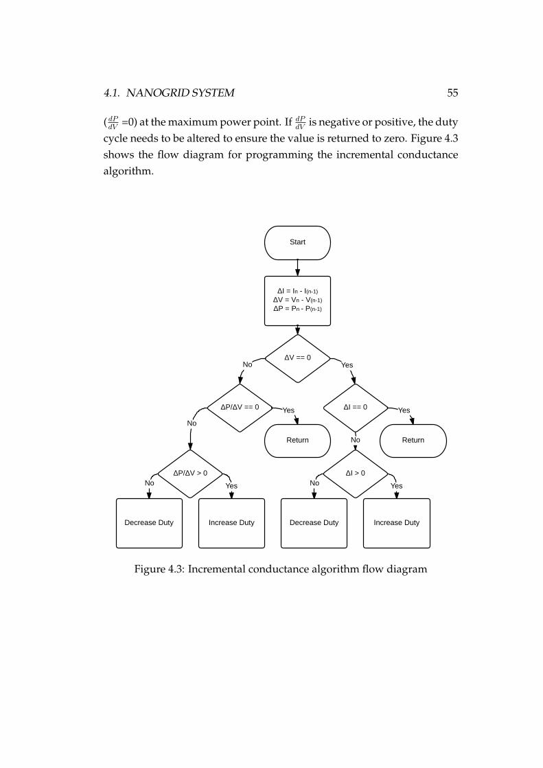
4.1. NANOGRID SYSTEM 55
( dPdV
=0) at the maximum power point. If dPdV
is negative or positive, the dutycycle needs to be altered to ensure the value is returned to zero. Figure 4.3shows the flow diagram for programming the incremental conductancealgorithm.
Start
? I = In - I(n-1) ?V = Vn - V(n-1) ?P = Pn - P(n-1)
?V == 0
?I == 0?P/?V == 0
Return
?I > 0
Increase DutyDecrease Duty
Return
?P/?V > 0
Increase DutyDecrease Duty
Yes
Yes
No
YesNo
Yes
No
No
YesNo
Figure 4.3: Incremental conductance algorithm flow diagram

56 CHAPTER 4. NANOGRID CONTROL SYSTEM
Constant voltage output
While altering the duty cycle of the interleaved boost converter, to ensureoperation at the maximum power point delivers the desired result at theinput, the output voltage has the potential to vary over a large range. Forthis reason a buck converter is cascaded with the interleaved boost con-verter enabling the system to output a constant voltage (380V ).A synchronous buck converter was selected to achieve this due to its highefficiency and low component count (when compared to alternative DC-DC converters e.g. SEPIC) [199]. Figure 4.4 shows the schematic of thebuck converter, equation (4.5) was used to select the required inductor.Equation (4.6) was then used to calculate the capacitor value for the re-quired output voltage ripple. However, in order to size the capacitor cor-rectly for transient response, a larger capacitor was required which wascalculated with equation (4.7) (variables for equations (4.5), (4.6) and (4.7)explained in table 4.2) [200, 201].
L =VOut × (VIn − VOut)
∆IL × fs × VIn(4.5)
COutmin=
∆IL8× fs ×∆VOut
(4.6)
COutmin=
L× I2LMAX
(VOut + VOS)2 − V 2Out
(4.7)
The feedback controller was designed as outlined in [202]. Equations(4.8) and (4.9) were used to locate the poles and zeros of the system andf0 was set to a tenth of the switching frequency. This allowed the use of atype 2 proportional-integral (PI) feedback loop as the conditions in (4.10)were met. Rf1 was set to an arbitrary value in the low kΩ range, andthe remaining variables were calculated using equations (4.11) through(4.14) (ESR is the equivalent series resistance ofCOut, Vref is the feedback’s
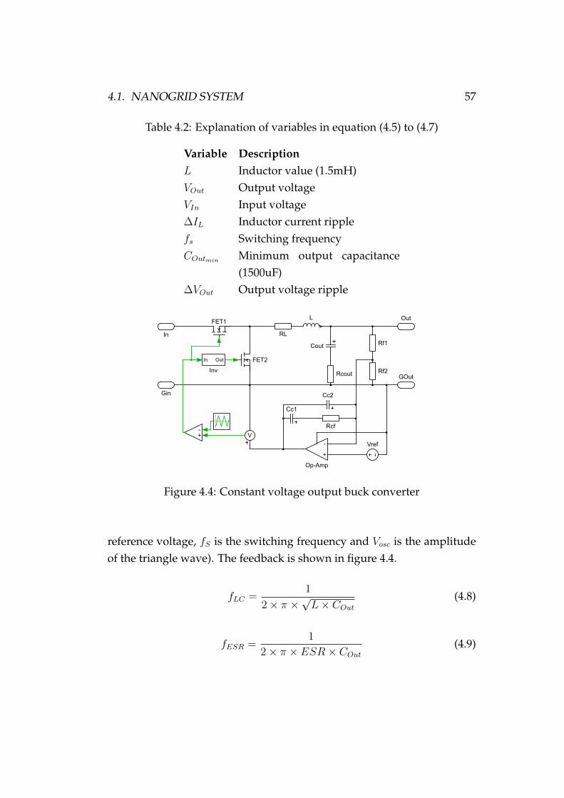
4.1. NANOGRID SYSTEM 57
Table 4.2: Explanation of variables in equation (4.5) to (4.7)
Variable DescriptionL Inductor value (1.5mH)VOut Output voltageVIn Input voltage∆IL Inductor current ripplefs Switching frequencyCOutmin
Minimum output capacitance(1500uF)
∆VOut Output voltage ripple
Figure 4.4: Constant voltage output buck converter
reference voltage, fS is the switching frequency and Vosc is the amplitudeof the triangle wave). The feedback is shown in figure 4.4.
fLC =1
2× π ×√L× COut
(4.8)
fESR =1
2× π × ESR× COut
(4.9)

58 CHAPTER 4. NANOGRID CONTROL SYSTEM
fLC < fESR < f0 <fS2
(4.10)
Rf2 =Rf1 × VrefVOut − Vref
(4.11)
RC1 =Rf1 × fESR × Vosc × f0
Vin × f 2LC
(4.12)
CC1 =1
1.5× π ×RC1 × fLC(4.13)
CC2 =1
π ×RC1 × fs(4.14)
MPPT Nanogrid Control Application
To demonstrate the MPPTs ability to function as a control signal for thenanogrid control system, Figure 4.5 and Figure 4.6 display a simulatedtest scenario with a constant solar irradiance (1000W/m2) under varyingload conditions. Figure 4.5 shows the schematic of a PV array (with themaximum output power of 3120W ), the interleaved boost converter cas-caded with the constant voltage converter supplying three loads. It canbe seen in Figure 4.6 that initially the system draws 320W of power, at 1minute it draws 2kW , at 2 minutes 4kW before returning back to 320W atthe 3 minute mark. This shows that the maximum power signal remainsunchanged even when the PV power production is exceeded by the loadand the grid must supply the deficit power.
Figure 4.7 shows the PV output power and the output voltage of theconstant voltage converter under a number of solar irradiance conditions.The 380V system output has an initial transient lasting 0.3s after whichit remains within its 0.4V ripple, even during large irradiance transitions.The MPPT has an initial transient that lasts for 0.35s, it settles within 0.15s
on transitions after this point. Both the MPPT and constant voltage outputare unaffected by changes in output load.

4.1. NANOGRID SYSTEM 59
PVStringR1
Cin Cout
L
D
Rcin
RL
Rcout
L1
RL1 D1
MPPTIinVin
OutOutinv
SenseVI
Cout1
L2
RL2
Rcout1
Inv
In Out
Rf1
Rf2
Op-Amp
+
-
Vref
Cc2
Cc1
Rcf+-
V
Grid/RectifiedR2 R3
Figure 4.5: PV module, MPPT, constant voltage converter and grid feeding3 loads
Figure 4.6: MPPT output under load varying conditions
4.1.2 Central and Node Controllers
The system control is distributed across the central controller and multi-ple control nodes. The central controller has a coordinating role within thecontrol scheme gathering information from the MPPT and nodes, facilitat-ing interactions.
The system’s control nodes are split into two categories; standard house-hold loads and thermostatically controlled household loads. Category onecontrol nodes utilise current and voltage sensors to monitor the power

60 CHAPTER 4. NANOGRID CONTROL SYSTEM
Figure 4.7: Test solar irradiance (top), MPPT input power (middle) andconstant voltage out (bottom)
draw of each standard household load, have the ability to switch the loadson/off when required and implement the control delegated by the cen-tral controller. The second category of the control nodes, associated withthe thermostatically controlled loads, not only implement the categoryone functions but are also equipped with temperature sensing capabili-ties. They also have the ability to vary the power consumed by the ther-mostatically controlled loads via a DC to DC step down converter (Buck

4.1. NANOGRID SYSTEM 61
converter). These capabilities are used by the nanogrid to distribute ade-quate power to the thermostatically controlled loads, ensuring the controlscheme and save operation of the load is implemented.
Control Node
Within the nanogrid, it was favourable to implement control law prior tothe load drawing power from the main nanogrid supply. To do so, a con-trol node was developed with the ability to observe a loads behaviour, re-port back to the nanogrid central controller and receive instructions beforethe associated load began drawing power.
Figure 4.8 shows a basic block diagram of the node, where the DC sup-ply and load is equivalent to the nanogrid’s DC bus and a household ap-pliance respectively. The node’s hardware consists of three switches (inthis case p-channel MOSFETs) and storage in the form of a capacitor bank(capacitor bank selected rather than batteries to allow various voltage val-ues to be used). The switches are controlled by a microcontroller whichmonitors the current and voltage of the capacitor bank and node’s output,making localised control decisions based on these variables. The micro-controller also sends and receives information to/from the central con-troller, relaying the load’s status and implementing control designated bythe nanogrid.
Figure’s 4.9 through 4.12 show the functionality of the node with anexplanation of each operating mode given below.
• Charge mode: The node utilises a capacitor bank to store charge whichis used to supply a load with power momentarily while control de-cisions are made by the nanogrid. The microcontroller monitors thevoltage level of the capacitor bank. If the capacitor bank drops belowa predetermined level (eg 23.8V on a 24V line), due to leakage cur-rent or load activity, the “charge switch” (P1) is activated until thevoltage returns to an adequate level. While this occurs, the capacitor

62 CHAPTER 4. NANOGRID CONTROL SYSTEM
DC
P3
P3
P3
Load
Capacitor bank
ToMicro To
Micro
ToMicro
P1 P2
P3
Figure 4.8: Node Block diagram
bank to load switch (P2) is set to “off” to ensure the load is not ser-viced via this route. The supply to load switch (P3) is switched “off”unless the conditions outlined in the supply to load mode are met. Ifthis occurs, P3 will be switched “on”, P2 will remain “off” and P1
will continue to charge the capacitor bank when necessary. A blockdiagram of the charge mode procedure is shown in figure 4.9, withthe current path displayed in red.
• Capacitor bank to load idle mode: Once the capacitor bank is charged,P2 is switched “on” ready for the load to be switched on. The outputcurrent and voltage is monitored, and while no current is drawn,the node will remain in this idle state. Figure 4.10 displays a blockdiagram of this mode.
• Capacitor bank to load draw mode: Once the load is switched on, it be-gins to draw current from the capacitor bank. The microprocessorwill note the current draw and voltage level on the output of the

4.1. NANOGRID SYSTEM 63
DC
P3
P3
P3
Load
Capacitor bank
ToMicro To
Micro
ToMicro
P1 P2
P3
Figure 4.9: Node Block diagram
DC
P3
P3
P3
Load
Capacitor bank
ToMicro To
Micro
ToMicro
P1 P2
P3
Figure 4.10: Node Block diagram

64 CHAPTER 4. NANOGRID CONTROL SYSTEM
node, calculating the load’s power draw. This information is thensent to the central controller and instruction is awaited. The Capaci-tor bank to load draw mode is shown in figure 4.11
DC
P3
P3
P3
Load
Capacitor bank
ToMicro To
Micro
ToMicro
P1 P2
P3
Figure 4.11: Node Block diagram
• Supply to load mode: At this stage a signal is received by the nodefrom the central controller, confirming or denying the availability ofpower. If there is not adequate power available to operate the load,P3 will remain off. However, if power is available (or made availableby the central controller), P3 is switched on and the power is pulledfrom the supply as shown in figure 4.12. As previously discussed, P2
will remain off during this procedure, allowing the capacitor bank tocharge. Once the output current draw is returned to zero, the systemwill reset, returning to “charge mode”.
Figure 4.13 shows the simulated results of a node supplying a 48V,250W load which switches on at t = 10 minutes. The capacitor bank ini-tially supplies the load while the nanogrid controller assesses the availabil-

4.1. NANOGRID SYSTEM 65
DC
P3
P3
P3
Load
Capacitor bank
ToMicro To
Micro
ToMicro
P1 P2
P3
Figure 4.12: Node Block diagram
ity of power. Once it is established that the nanogrid has adequate power,the nanogrid begins to supply the load at which point the capacitor bankis recharged. During this transaction (as shown in the top plot of figure4.13 ), the capacitor voltage drops to 47.78V while the capacitor suppliesthe load (a drop of approximately 0.42% and well within an acceptablemargin).
Thermostatically controlled load nodes
The thermostatically controlled loads node has an additional feature al-lowing the nanogrid controller to vary the power consumed by the load.This is implemented by a buck converter which varies the voltage to thethermostatically controlled load (in turn altering the power). The designprocess follows that of the buck converter utilised by the MPPT minus theclosed loop feedback control. The duty cycle instead is controlled directlyby the control scheme based on a number of variables discussed in section
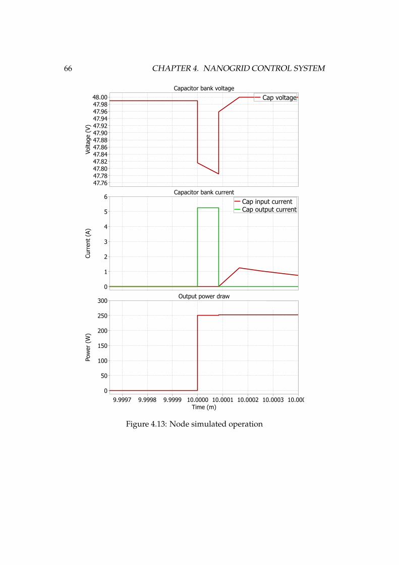
66 CHAPTER 4. NANOGRID CONTROL SYSTEM
Capacitor bank voltage
Capacitor bank current
Output power draw
Voltage (
V)
47.7647.7847.8047.8247.8447.8647.8847.9047.9247.9447.9647.9848.00
Curr
ent
(A)
0
1
2
3
4
5
6
Time (m)
9.9997 9.9998 9.9999 10.0000 10.0001 10.0002 10.0003 10.0004
Pow
er
(W)
0
50
100
150
200
250
300
Cap voltage
Cap input currentCap output current
Product
Figure 4.13: Node simulated operation

4.2. THERMOSTATICALLY CONTROLLED LOADS 67
4.2.1. Figure 4.14 shows a block diagram of the thermostatically controlledloads node.
DC
P3
P3
P3
Load
Figure 4.14: Thermostatically controlled load node
4.2 Thermostatically Controlled Loads
The nanogrid makes use of household loads with a thermal output, rely-ing on their relatively slow dynamics to store energy which can be usedoutside of PV production times. During the design of the nanogrid, threethermostatically controlled loads were identified as large/frequent con-sumers of power and selected for analysis and control. These were theelectric water heater, refrigerator and space heating, for which the analy-sis and control theory are presented below.
4.2.1 Water and Space Heating
It makes sense to discuss the water and space heating collectively, as thecontrol strategies are connected. The water heater considered in this re-search is the common domestic electric hot water storage tank, while the

68 CHAPTER 4. NANOGRID CONTROL SYSTEM
space heating is implemented by a storage heater (sometimes referred toas “night storage heaters”). Each load is presented below, before the con-trol strategy is discussed.
Water Heater
Heating water for use in showers and the sink requires an electric waterheater to operate for hours each day (the time depending on hot wateruse), typically drawing power in excess of 2kW . This makes it one of thelargest household loads and when controlled, gives it the potential to shifta substantial portion of the daily consumption. The water heater’s ther-mal behaviour is governed by the differential Eqn. (4.15) [203], with thevariables explained in Table 4.3.
McdTWdt
= mc(Ti − TW )− hA(TW − Ta) + q (4.15)
Eqn. (4.15) can be rearranged to calculate the change in temperatureover a specific time period (4.16), and from here, the change in time fora specific temperature change can be derived (4.17). With Eqn. (4.17), thethermal autonomy (time the water temperature can remain above a pre-determined threshold) of the water heater can then be calculated, as canthe time required to heat the water to an upper temperature threshold.As the temperature difference between the upper and lower temperaturethreshold increases, the time between “on” cycles (Ton) also increases.
This property can be utilised in the design of the nanogrid controllerby bypassing the standard thermostat and selecting an upper/lower wa-ter temperature to give the desired on/off time interval. In the nanogridcontroller simulated for this work, 81C was selected as the upper tem-perature while 55C was selected for the lower, giving 24 hours thermalautonomy (while m = 0).
Figure 4.15 displays the water heater’s thermal autonomy plotted against

4.2. THERMOSTATICALLY CONTROLLED LOADS 69
Table 4.3: Explanation of variables in Eqn. (4.15)
Variable Description Simulation ValuesM Mass of water (kg) 88L to 300Lc Specific heat of the water (J/kgC) 4179 J/kgCm Flow rate (kg/h) 9L/mTW Temperature of the water in the tank
(C)55C to 81C
Ti Temperature of the water entering thetank (C)
7C
h Heat transfer coefficient (for convec-tion to ambient) (W/m2C)
1.5W/m2C
A Area of the tank (m2) 1.84m2 to 3.85m2
Ta Ambient temperature (C) 20C
q Heat rate of the heating element (W ) 2kW to 3kWt time (s)
water consumption for a variety of initial temperatures.
Hot Water Consumption (L)0 10 20 30 40 50 60 70 80 90 100
Tim
e of
Aut
onom
y (h
ours
)
0
5
10
15
20
25Water Heater Time of Autonomy
81°C75°C70°C65°C60°C
Length of shower (minutes)0 2 4 6 8 10 12
Tim
e of
Aut
onom
y (h
ours
)
0
5
10
15
20
2581°C75°C70°C65°C60°C
Figure 4.15: Initial water temperature and its thermal autonomy vs waterconsumed

70 CHAPTER 4. NANOGRID CONTROL SYSTEM
TW =aTi + dTa + q
a+ d+ ke−(a+d
b)t (4.16)
where a = mc, b = Mc and d = hA.
t =b× log(x)
a+ d(4.17)
where x =k
TW − fand f =
aTi + dTa + q
a+ d, with k being the integration
constant.
Increasing the upper temperature of the water to 81C raises safety is-sues, as temperatures at this level can scald users. To counteract this neg-ative effect, it is recommended that a thermostatic mixing valve is addedto the output of the hot water tank. This device mixes cold with hot waterto give a constant (safe) output water temperature, and will switch off thehot water in the absence of cold. It should also be noted, from eqn. (4.15),that with the increased water temperature, the loss to ambient will alsoincrease. However, if the heat transfer coefficient (h) is altered by addinginsulation to the water heater (eg insulating blanket), these losses can benegated [204].
Storage Heater
Initial tests were conducted with the hot water tank and refrigerator con-trolled by the nanogrid. It was found that, although the solution produceda reduction in external power consumed by the nanogrid, space heatinglimited its effectiveness. This motivated the inclusion of space heatinginto the control regime.
A storage heater, consisting of elements heating insulated bricks (asshown in Figure 4.16), was selected for the solution due its high thermalautonomy. The bricks are heated during times of high PV production and

4.2. THERMOSTATICALLY CONTROLLED LOADS 71
the heat is stored until it is required, at which stage a fan is activated toachieve the required room temperature. If there has been insufficient PVproduction to heat the bricks during a single day, the heater draws therequired power at time of use (from the grid).
Insulation
Brick Heat Storage
Element
Fan
Vent
Figure 4.16: Storage Heater Diagram
Eqn. (4.18) describes the behaviour of the storage heater, eqn. (4.19)shows the losses during fan “off/on” operation (where QOut increaseswith the temperature of the bricks) and eqn. (4.20) displays the inputpower [205]. The variables of the storage heater equations are outlinedin Table 4.4.
MbcbdTbdt
= QIn −QOut (4.18)

72 CHAPTER 4. NANOGRID CONTROL SYSTEM
QOut =
Qfb +Qs +Qvn Fan off
Qfb +Qs +Qvf Fan on
(4.19)
QIn =
R× i2 Charge
0 Discharge
(4.20)
Table 4.4: Explanation of variables in Eqn. (4.18), (4.19) and (4.20)
Variable Description Simulation ValuesMb Mass of the bricks (kg) 60kgcb Specific heat of the bricks
(J/kgC)670J/kgC
Tb Temperature of the bricks (C) 20C to 600C
Qfb Insulated front and back con-duction losses
See table 4.5
Qs Insulated side, top and bottomconduction losses
See table 4.5
Qvn Natural convection via fan out-let
Temperature dependant
Qvf Forced convection via fan outlet Temperature dependantR Resistance of heating elements
(Ω)26.4Ω
i Current through heating ele-ments (A)
8.7A
Eqns. (4.18), (4.19) and (4.20) need to be expanded and rearranged tocalculate the time of autonomy under fan off/on conditions. The deriva-tions for the “Fan off”, then “Fan on”, are as follows:

4.2. THERMOSTATICALLY CONTROLLED LOADS 73
Fan off: During fan off times, the area where the fan extracts the heatis still exposed so must be considered as a natural convection output. Thisis the main point of loss for the storage heater and can cause a room’stemperature to raise during the charge cycle. The variables used in Eqn.(4.21) to explain the operation of the fan off cycle, are shown in Table 4.5.The equation is then rearranged in (4.22) and (4.23).
MbcbdTbdt
= QIn −kfbAfb
lfb∆T − ksAs
ls∆T − kvnAvn∆T (4.21)
where ∆T is temperature of the bricks (Tb) minus the temperature of theroom (TR).
Table 4.5: Explanation of variables in equation 4.21
Variable Description Simulation Valueskfb Thermal conductivity of front and
back (W/mC)0.021W/mC
Afb Area of the front and back (m2) 0.698m2
lfb Thickness of the front and back (m) 0.009mks Thermal conductivity of the
sides/top/bottom (W/mC)0.04W/mC
As Area of the sides/top/bottom (m2) 0.345m2
ls Thickness of the sides/top/bottom(m)
0.05m
kvn Natural convection heat transfer coef-ficient (W/m2C)
10.45W/m2C
Avn Heat transfer area of the surface (m2) 0.034914m2
Tb =QIn + (a+ b+ c)TR
a+ b+ c+ we−(a+b+c)t (4.22)
t =log( w
Tb−p)
a+ b+ c(4.23)

74 CHAPTER 4. NANOGRID CONTROL SYSTEM
where a =kfbAfb
lfbMbcb, b =
ksAs
lsMbcb, c =
kvnAvn
Mbcb,
p =QIn + (a+ b+ c)TR
a+ b+ cand w is the constant of integration.
Fan on: During the fan on cycle, the natural convection losses areexchanged to forced convection losses extracting heat from the storageheater at a much faster rate. This can be controlled by a room thermostat,ensuring the temperature of the room is adequate.
The variables in Eqn. (4.24) can be taken from Table 4.5 with the excep-tion of kvf which is the forced convection heat transfer coefficient, and Avf
is equal in area to Avn.
MbcbdTbdt
= −kfbAfb
lfb∆T − ksAs
ls∆T − kvfAvf∆T (4.24)
where ∆T is temperature of the bricks (Tb) minus the temperature of theroom (TR). Eqn. (4.25) and (4.26) make time the focus in order to calculatethe storage heater’s thermal autonomy.
Tb = TR + we−(a+b+d)t (4.25)
t =log( w
Tb−TR)
a+ b+ d(4.26)
where a =kfbAfb
lfbMbcb, b =
ksAs
lsMbcb, d =
kvfAvf
Mbcband w is the constant of inte-
gration.
Water/Storage Heater Control Strategy
The water and storage heater control strategy looks to maximise PV powerconsumed, store the energy until required and ultimately reduces the ex-ternal power consumed by the nanogrid.
As the electric elements in both the water and storage heaters are resis-tive, it allows each load’s power consumption to be varied as required by
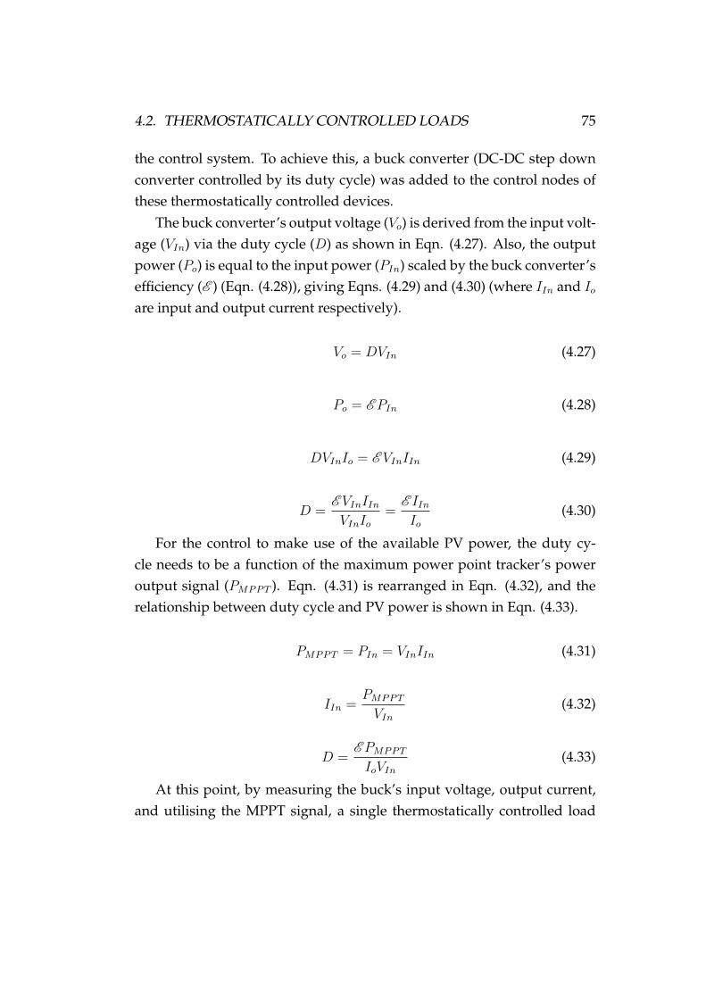
4.2. THERMOSTATICALLY CONTROLLED LOADS 75
the control system. To achieve this, a buck converter (DC-DC step downconverter controlled by its duty cycle) was added to the control nodes ofthese thermostatically controlled devices.
The buck converter’s output voltage (Vo) is derived from the input volt-age (VIn) via the duty cycle (D) as shown in Eqn. (4.27). Also, the outputpower (Po) is equal to the input power (PIn) scaled by the buck converter’sefficiency (E ) (Eqn. (4.28)), giving Eqns. (4.29) and (4.30) (where IIn and Ioare input and output current respectively).
Vo = DVIn (4.27)
Po = EPIn (4.28)
DVInIo = E VInIIn (4.29)
D =E VInIInVInIo
=E IInIo
(4.30)
For the control to make use of the available PV power, the duty cy-cle needs to be a function of the maximum power point tracker’s poweroutput signal (PMPPT ). Eqn. (4.31) is rearranged in Eqn. (4.32), and therelationship between duty cycle and PV power is shown in Eqn. (4.33).
PMPPT = PIn = VInIIn (4.31)
IIn =PMPPT
VIn(4.32)
D =EPMPPT
IoVIn(4.33)
At this point, by measuring the buck’s input voltage, output current,and utilising the MPPT signal, a single thermostatically controlled load

76 CHAPTER 4. NANOGRID CONTROL SYSTEM
(e.g. water heater) could consume all of the available PV power withoutexceeding its capacity.
However, to be effective, this control concept is expanded to includestandard household loads and interactions between the water and storageheaters. Eqn. (4.34) expands on Eqn. (4.33) to include data from the cen-tral controller (Ltotal), accounting for the power consumed by the standardhousehold loads. It also adds a multiplier (m), which is used to calculatethe ratio of PV power received by the water and storage heaters based ontheir “urgency”.
Dratio = mE (PMPPT − Ltotal)
IoVIn(4.34)
The measure of urgency is derived from the thermal autonomy of theheaters (water or storage). By inserting the current temperature of eachload in real time, into Eqns. (4.17) (water heater) or (4.23) (storage heaterfan off) and (4.26) (storage heater fan on), the time until the next “on” cy-cle is calculated (toff ). In the same manner, the time required to heat theload to its upper limit could also be calculated with the above mentionedequations (ton). Multiplying the time required to heat the load by its powerdraw (“P”, which at this stage is manually entered from datasheet infor-mation with continued research on automating a calibration process), andconsidering the ratio of on/off cycles in a single day, the urgency of theload is calculated as shown in Eqn. (4.35). By giving preference to the mosturgent loads, the control strategy operates on the load which is likely todraw the most power outside of PV production times.
x = Pton
ton + toff/day (4.35)
Once the measure of urgency is calculated, the ratio term (m..) canbe derived for the water and storage heaters as shown in Eqn. (4.36).This means 100% of the power produced by PV can now be consumedby household loads, and the more urgent thermostatically controlled load

4.2. THERMOSTATICALLY CONTROLLED LOADS 77
(out of the water and storage heater) is serviced with the majority of theremaining PV power.
m.. =
xWH
xWH + xSHWater Heater
xSHxWH + xSH
Storage Heater(4.36)
To ensure the safety and comfort of the users, there were exceptions tothe control law discussed above. These are as follows:
• Water Lower Temperature Threshold The water stored in the water heatermust stay above the temperature at which legionella bacteria canbreed. For this reason, if the temperature drops below 55C, the wa-ter heater’s element will turn on regardless of PV power availability.If PV power is not available, the water is heated to a lower temper-ature threshold (60C) and is only heated to upper limit threshold81C once PV power is available.
• Room Temperature The storage heater will be required to keep theroom at a specific temperature for a time period determined by theuser. If there has been insufficient PV power to heat the bricks to atemperature at which the storage heater can sustain the user’s re-quirements, additional power will be needed. As with the waterheater, the storage heater will draw power regardless of PV avail-ability to ensure the room is kept at the appropriate temperature.
• Upper Temperature Limits Both the water and storage heater have up-per temperature limits under which the devices can operate safely.If these limits are reached and PV power is still available, the load isallowed to cool to an upper temperature threshold before it is heatedagain. If the upper limit is reached and PV power is no longer avail-able, the temperature will be allowed to reach its lower limit.
Figure 4.17 shows the flow diagram of a typical interaction between a non-thermostatically controlled load and a thermostatically controlled load. In

78 CHAPTER 4. NANOGRID CONTROL SYSTEM
this situation, the former load is switched on by a user and the latter aresponse to the change in household consumption.
MPPT Controller replies with available
PV capacity
Central Controller requests operating status from MPPT
Non-thermostatically controlled load is
switched on
Non-thermostatically controlled Node requests power
Central Controller relays the PV capacity to the thermostatically controlled load’s
node
If the load’s thermal characteristics allow, power to the load is
altered to fit the MPPT and
Non-thermostatically controlled load
The thermostatically controlled load’s
node observes the thermal
characteristics of the load
Central Controller replies to the
Non-thermostatically controlled node’s
request, allowing the load to draw power
Figure 4.17: Flow diagram of a typical load interaction
4.2.2 Refrigerator
Although the refrigerator is not a large load compared to the water heater,it is far more frequent and its power draw is characterised by a large cur-rent spike on start up (due to the compressor). This is also the reason therefrigerator cannot take part in the buck style control system developed

4.2. THERMOSTATICALLY CONTROLLED LOADS 79
for the water and space heating. However, as the refrigerator is a thermo-statically controlled load, it can still help to reduce the power consumedby the nanogrid (from an external source).
The thermal characteristics are described by Eqn. (4.37) (with variablesexplained in Table 4.6) a first order piece-wise approximation where Case0 is when the refrigerator is OFF and Case 1 when it is ON [206].
dTFdt
=
Ta − TFCcRi
Case 0
TaCcRi
+Te
CcRec
− TFCcRiRec
Case 1
(4.37)
Table 4.6: Explanation of variables in Eqn. (4.37)
Variable DescriptionTF Cabinet temperatureTa Ambient temperatureTe Inlet temperature of the refrigerant evaporatorCc Heat storage capacityRi Thermal resistance of the insulationRec Thermal resistance of the wall between the cabinet and evaporator
As with the water heater, this equation can be rearranged to calculatetemperature change (4.38) and the change time (4.39). The time equationis used to create a control algorithm to manipulate the thermal autonomyof the refrigerator.
TF =
Ta + ke
1CcRi
tCase 0
z (TaCcRi
+Te
CcRec
) + ke1zt Case 1
(4.38)
where z = CcRiRec, k is the constant of integration, and the time taken tocool/heat the refrigerator cavity is given by:

80 CHAPTER 4. NANOGRID CONTROL SYSTEM
tcool/heat =
CcRi log(
k
TF − Ta) Case 0
z log(k
TF − z( Ta
CcRi+ Te
CcRec)) Case 1
(4.39)
where z = CcRiRec and k is the constant of integration.
Refrigerator Control Algorithm
The goal of the refrigerator control is to reduce the frequency of “on”time while PV power is unavailable. Figure 4.18 shows a flow diagramof the algorithm (variables explained in table 4.7). In the algorithm thereis a lower/upper threshold temperature, 1C and 2.4C respectively, andlower/upper limit temperature (0C and 4C respectively).
If sufficient PV power is available to accommodate the refrigerator’spower requirements, the refrigerator is cooled to the lower limit where itoscillates between the lower limit and lower threshold. If there is insuffi-cient power for the refrigerator, the temperature is allowed to increase tothe upper limit and oscillates between the upper limit and upper thresh-old.
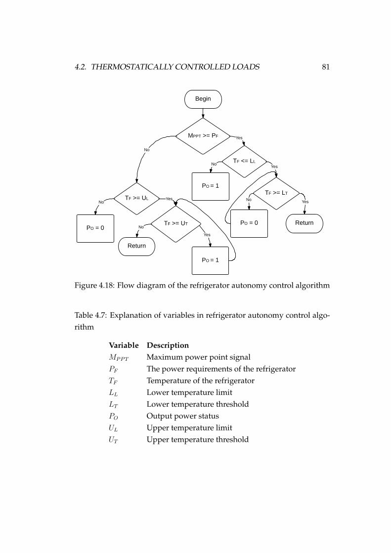
4.2. THERMOSTATICALLY CONTROLLED LOADS 81
Begin
MPPT >= PF
TF <= LL
TF >= UL
Yes
YesNo
TF >= UT
YesNo
No
No
PO = 1TF >= LT
No Yes
PO = 0 ReturnPO = 0
Return
PO = 1
Yes
Figure 4.18: Flow diagram of the refrigerator autonomy control algorithm
Table 4.7: Explanation of variables in refrigerator autonomy control algo-rithm
Variable DescriptionMPPT Maximum power point signalPF The power requirements of the refrigeratorTF Temperature of the refrigeratorLL Lower temperature limitLT Lower temperature thresholdPO Output power statusUL Upper temperature limitUT Upper temperature threshold

82 CHAPTER 4. NANOGRID CONTROL SYSTEM
4.3 Simulation, Results and Discussion
With the objective of the nanogrid being “to reduce grid power consumed, byutilising locally produced PV power”, a method of quantifying this outcomeneeded to be established. A model was developed in “PLECS” simula-tion software (an extension of Matlab’s Simulink), which consisted of thefollowing considerations:
• Relevant solar data: To ensure the nanogrid control was simulated un-der realistic conditions, the solar calculator developed by the Na-tional Institute of Water and Atmospheric research (NIWA) was used[207]. This calculator used 18 years of data from the nearest climatestation combined with local landscape to obtain an estimate of a re-gion’s solar energy. The selected location for the tests was Kelburnin Wellington, New Zealand (-41.29 latitude, 174.76 longitude). Toobserve the extreme ends of the available solar, a week of solar datafrom the middle of Summer and Winter was selected, Figure 4.19shows the selected weeks with the maximum power output of the6kW PV installation used for the simulations.
• Varied load curves It was important to test the nanogrid controllerunder a variety of load conditions to observe the controller’s be-haviour and to ensure a specific loadline did not produce a biasedresult. The model was designed so that multiple on/off times andpower draw of the household loads shown in Table 4.8 could be var-ied (along with the additional details discussed in the table) to cre-ate multiple household scenarios. Appendix A presents the on/offtimes for all loads used within the 10 houses, along with refrigera-tor parameters, shower times/lengths and hot water cylinder char-acteristics. With the exception of the refrigerator (which had an in-ductive element in the model), the loads were modelled as resistiveloads with curves derived from either; the behaviour of physically

4.3. SIMULATION, RESULTS AND DISCUSSION 83
measured loads (television, toaster, stereo, kettle, refrigerator, hotwater tank, heater), responses from literature (dishwasher) [208] orassumed responses for smaller loads (lights, lamps, phone charger,computer/laptop, alarm clocks). Ten household curves were thendesigned to test the nanogrid controller as shown in Figure 4.20. Inthis figure, the blue block area depicts the kWh consumption of thesummer load, while the red block area the winter (note the red blockis consumption additional to the blue). The red lines in the figuredisplay the instantaneous summer consumption, while the blue linesthe instantaneous winter (kW).
• Comparison between controlled and uncontrolled: Two versions of eachof the ten households were developed, one with the nanogrid con-troller and the other without control. These were then tested underthe varied solar irradiance condition with an identically sized PV ar-ray, MPPT (to ensure the output of the PV array was comparable)and grid connection. The power consumed from the grid by eachscenario was monitored in order to validate the nanogrid’s ability tomeet its objective.
Figure 4.21 shows the simulation setup of a typical house within thePLECS modelling environment.
The results shown in Table 4.9 (Winter) and 4.10 (Summer) give a com-parison between the power consumed from the grid by the controlled anduncontrolled nanogrid in kWh consumed per day, and the reduction ofpower consumed as a percentage.
The results show that as a percentage, the reduction of power con-sumed from the grid during the summer (in this geographic location) isgreater than in winter. However, because the household consumption ismuch larger in the winter (than in summer), the reduction of power con-sumed from the grid is more significant during this season.

84 CHAPTER 4. NANOGRID CONTROL SYSTEM
Table 4.8: Loads within the modelled house
Variable DescriptionLights Six availableLamps Three availablePhone charger Three availableComputer/Laptop Three availableAlarm clocks Two availableShowers Variable time and length of showers (9L/m flow rate)Sink Variable hot water used for dishes etc (L)Hot water tank Variable water capacity, physical sizeDishwasher Full cycleRefrigerator Variable initial tamp, thermostat high and low tempOven Four separate elements and/or ovenHeater Bar heater considered for uncontrolled houseStorage heater Outdoor temperature varied throughout day/nightkettle Heating 1LToaster On time 3 minutesTelevision Single availableStereo Single available
Figure 4.22 shows a controlled and uncontrolled household’s consump-tion over a 24 hour period in winter. It can be seen here that the con-trolled system consumes a large percentage of the available PV power(blue shaded area), in turn reducing grid power consumption. In compar-ison, for the majority of the uncontrolled PV production time, little morethan the refrigerator is operating.
While this plot does not represent the consumption of every house-hold, every day, it does depict the general trend and shows how the algo-rithm achieves its reduction in power consumed.
To get an idea of the potential reduction in power consumed from the

4.3. SIMULATION, RESULTS AND DISCUSSION 85
Figure 4.19: PV output power
grid delivered by the system over a year, figure 4.23 was plotted. Thisconsiders the load curve of house 1 operating under the average solar ir-radiance for a day of each month of the year (provided by NIWA [207]).The PV capacity was varied from 500W to 10kW for both the controlledand uncontrolled operating conditions, and the power consumed fromthe grid was observed. It can be seen that for lower PV capacities, thereduction is not as drastic as 5kW and above where the reduction settlesat approximately 44%.

86 CHAPTER 4. NANOGRID CONTROL SYSTEM
Table 4.9: Comparison of power consumed by controlled and uncontrolledhouseholds in Wellington, NZ during Winter
House Uncontrolled kWh/day Controlled kWh/day Reduction %1 15.94 8.89 44.212 19.78 13.89 29.763 18.31 11.31 38.254 15.75 8.89 43.545 32.72 25.39 22.386 24.12 13.58 43.687 21.16 10.28 51.438 21.17 11.69 44.819 17.76 9.18 48.3410 11.14 5.45 51.06Ave % 41.75
Table 4.10: Comparison of power consumed by controlled and uncon-trolled households in Wellington, NZ during Summer
House Uncontrolled kWh/day Controlled kWh/day Reduction %1 8.42 4.18 50.402 11.54 8.53 26.043 7.66 3.24 57.664 5.02 1.91 61.865 7.33 4.71 35.846 11.13 7.07 36.487 6.68 3.08 53.898 8.46 4.46 47.339 9.68 5.36 44.6110 7.08 3.27 53.88Ave % 46.80

4.3. SIMULATION, RESULTS AND DISCUSSION 87
Figure 4.20: Uncontrolled household consumption curves displayed in in-stantaneous (lines) and kWh (blocks)

88 CHAPTER 4. NANOGRID CONTROL SYSTEM
Ch
arg
er1
Ch
arg
er2
Grid
NL
Sens
N1C1
Node1
NL
Sens
N2C2
Node2
NL
Sens
N3C3
Node3
NL
Sens
N4C4
Node4N
LSens
N5C5
Node5
NL
Sens
N6C6
Node6
NL
Sens
N7 C7Node7
NL
Sens
N8 C8Node8
NL
Sens
N9 C9Node9
NL
Sens
N10 C10Node10
NL
Sens
N12 C12Node12
NL
Sens
N13 C13Node13
NL
Sens
N14 C14Node14
NL
Sens
N15 C15Node15
NL
Sens
N16 C16Node16
NL Sen
s
N17
C17
Node17
NL Sen
s
N18
C18
Node18
NL Sen
s
N19
C19
Node19
NL Sen
s
N2
0C
20
Node20
NL Sen
s
N2
1C
21
Node21
NL Sen
s
N2
2C
22
Node22
TroomHeater
SensSw
InO
ut
N23C23
Node23
N1N2N3N4N5N6N7N8N9
N10N11N12N13N14N15N16N17N18N19N20N21N22N23N24
C1C2C3C4C5C6C7C8C9C10C11C12C13C14C15C16C17C18C19C20C21C22C23C24
NanogridController
WaterControlHotFlowRate WaterUseTw
WaterUse
TWH
NP
N24C24
Node24
Heater
BrickTempOutTroomFan_Heater
P
L Tb
TR
F_H
N
N11C11Node11
In
Tc_OutP
Vin
Sw
HotWaterTankNew
Massflowrate
TwP
IO
GW
IO
MPPT
PV
Figure 4.21: Schematic of PLECS simulation set up

4.3. SIMULATION, RESULTS AND DISCUSSION 89
Figure 4.22: Comparison of controlled and uncontrolled households overa 24 hour period in Winter

90 CHAPTER 4. NANOGRID CONTROL SYSTEM
Figure 4.23: Yearly reduction in power consumed by house 1 under variedPV capacities

4.4. CHAPTER SUMMARY 91
4.4 Chapter Summary
This chapter presents a novel nanogrid control strategy designed to re-duce grid power consumed by a single house or small building. Thisis achieved by utilising thermostatically controlled loads, storing energywhile PV power is available to be used when little to no PV power ispresent.
The nanogrid controller implements MPPT to achieve a high poweryield from the PV modules. It also uses the MPPT signal as a control input,enabling control decisions to be made based on available PV power. TheMPPT consists of an interleaved boost converter and control algorithm forwhich both the hardware and software design process is outlined. Theinterleaved boost converter’s output is then cascaded with a synchronousbuck converter to give the DC bus a constant 380V.
The nanogrid control topology is hybrid central control, with a centralcontroller coordinating interactions between control nodes which imple-ment real time load control. There are two types of control nodes whichboth sense the current and voltage applied to their associated load, withthe ability to switch off the load. The nodes that service the thermostat-ically controlled loads also have the ability to monitor temperature andmodulate the voltage to the load.
This chapter discusses the thermal characteristics of the three thermo-statically controlled loads the nanogrid controller uses to implement de-mand side management, namely the water heater, storage heater and re-frigerator. A control strategy for the water heater and storage heater ispresented that delegates a ratio of available PV power to each, taking intoconsideration the uncontrollable loads operating and the urgency of thethermostatically controlled loads. The urgency measure is derived fromthe thermal characteristics of the thermostatically controlled loads, calcu-lating which is expected to have the higher power draw over the day andensuring it receives adequate power. This control strategy alters the duty

92 CHAPTER 4. NANOGRID CONTROL SYSTEM
cycle of a buck converter embedded in the control node, altering the volt-age to the load and hence the power draw.
A control strategy for a refrigerator is also presented with the goal ofcontrolling the frequency of on/off cycles depending on the availability ofPV power. The control node achieves this by setting upper/lower temper-ature thresholds and limits, cooling the refrigerator to its lower limit whenPV power is available and allowing the temperature oscillate between thelower threshold and limit. When insufficient PV power is present, thetemperature of the refrigerator increases to its upper limit and oscillatesbetween its upper threshold and limit.
Ten daily household load curves are modelled to test the nanogrid con-troller’s ability to reduce grid power consumed. The ten houses are simu-lated with a week of winter and summer solar irradiance data, each testedwith and without the nanogrid controller. The consumption of grid poweris compared and it is found that on average, in winter the controller hasthe ability to reduce grid power consumed by 41.75% while in summer46.8%, giving a yearly average reduction of 44.28%.

Chapter 5
Interconnected NanogridNetwork
Nanogrids are often described as a ”bottom up” approach to power sys-tems due to their modular nature. This has the advantage of lending itselfto creating larger power systems by interconnecting multiple nanogrids,forming a microgrid structure as shown in Fig. 5.1. It focuses on a hi-erarchical approach to power distribution from nanogrid, to microgridand the national grid. This hierarchy utilises the semi-autonomous con-trol structures within the nanogrid to alleviate some of the stresses causedby intermittent power production/consumption (demand side manage-ment (DSM), supply side management (SSM)). These subsystems are theninterfaced to form the microgrid, adding further intelligence and creatingone bi-directional point of connection to the national grid. Power can thenbe shared between nanogrids via the network, decreasing the effects of anintermittent power supply while taking advantage of diverse power con-sumption patterns of the houses within the network. From the microgrid,power can be sold to, and/or bought from the national grid via the singlepoint of common coupling. The grid can then be used as a supplementarypower supply and incentives can be negotiated with the utility companiesto help stabilise the grid. The microgrid can also be advantageous to the
93

94 CHAPTER 5. INTERCONNECTED NANOGRID NETWORK
users during outages, with the ability to island from the national grid.
Figure 5.1: Microgrid made up of multiple nanogrids
This chapter explores the potential to reduce grid power consumedby a small cluster of interconnected houses. It introduces a novel controlscheme that uses the thermostatically controlled loads within the clusterof houses to increase the correlation between the total consumption andproduction of the microgrid. The maximum power point tracking signalis used to observe available PV power with the goal of servicing the high-est consuming loads within the cluster, ultimately reducing the amount ofgrid power consumed by the microgrid.
There are three scenarios of interest to establish if there is indeed anadvantage to implementing a combined control scheme. The first is anuncontrolled cluster of houses, the second individual nanogrid controlswithin the cluster, and the last is the combined control system. The grid

5.1. NANOGRID NETWORK SCENARIOS 95
power consumed by each of these structures is then compared to discoverwhich has the ability to reduce the cluster’s consumption by the largestamount.
5.1 Nanogrid Network Scenarios
In this section the topology of each scenario of interest is presented and ex-plained. An in-depth analysis of the equations that govern the power shar-ing within the combined control system (subsection 5.1.3) is also given.
5.1.1 Uncontrolled Nanogrid Network
The uncontrolled nanogrid network, shown in figure 5.2, is a cluster ofhouses with ability to share PV power produced before the point of com-mon coupling connects them to the grid. As the name would suggest,there is no control involved within the cluster of houses, other than themaximum power point tracker which gives an equivalent power sourcewhen comparing the three scenarios (for fair testing). The constant volt-age converter also performs its function, ensuring the cluster operates at380V DC.
While no control is implemented, it was found that implementing apoint of common coupling to the grid was advantageous to the reductionin grid power consumed. This is demonstrated in figures 5.3 and 5.4 wheretwo houses are producing 2.5kW of PV power, house one has a load whichexceeds this by 300W (2.8kW , between t = 2 and t = 5) and house twoconsumes 2kW (between t = 3 and t = 6). In figure 5.3 the two houses areconnected to the grid individually, and it can be observed that house onedraws the deficit 300W of power from the grid. In figure 5.4 the houseshave a point of common coupling before they are connected to the grid.This ensures the second house supplies the first with the required 300W

96 CHAPTER 5. INTERCONNECTED NANOGRID NETWORK
of power, alleviating the need to draw power from the grid. While thisis an “ideal” scenario to demonstrate how this interaction occurs, it wasfound to take place within the simulated household curves considered forthese tests (but difficult to display in an appropriate manner), typicallysupplying partial load consumption.
Grid
Converter
Constant Voltage
MPPT
Standard Load 1
StandardLoad ...
StandardLoad n
ThermoLoad ...
Constant Voltage
MPPT
Standard Load 1
StandardLoad ...
StandardLoad n
ThermoLoad ...
Constant Voltage
MPPT
Standard Load 1
StandardLoad ...
StandardLoad n
ThermoLoad ...
Figure 5.2: Microgrid made up of multiple nanogrids

5.1. NANOGRID NETWORK SCENARIOS 97
PowerConsumedbyHouse1
PowerConsumedbyHouse2
Power(W
)
0
500
1000
1500
2000
2500
Time(minutes)0 1 2 3 4 5 6 7 8 9 10
Power(W
)
0
500
1000
1500
2000
2500
GridPowerConsumedH1PVPowerH1PVCapacity
GridPowerConsumedH2PVPowerH2PVCapacity
Figure 5.3: Two individual uncontrolled house scenario showing gridpower consumed
PowerConsumedbyInterconnectHouse1
PowerConsumedbyinterconnectHouse2
Power(W
)
0
500
1000
1500
2000
2500
Time(minutes)0 1 2 3 4 5 6 7 8 9 10
Power(W
)
0
500
1000
1500
2000
2500
GridPowerConsumedH1PVPowerH1PVCapacity
GridPowerConsumedH2PVPowerH2PVCapacity
Figure 5.4: Two commonly coupled uncontrolled house scenario showingno grid power consumed

98 CHAPTER 5. INTERCONNECTED NANOGRID NETWORK
5.1.2 Individually Controlled Nanogrid Network
The individually controlled nanogrid network houses retain the same levelof control as discussed in chapter 4. Each house is equipped with a nanogridcontroller, ensuring the thermostatically controlled loads maximise the useof the available local PV power. The houses are connected, with the abil-ity to share power within the cluster before a point of common couplingconnects them to the grid. Each nanogrid controller knows only the pro-duction and consumption of the individual house, with no knowledge ofthe other houses within the cluster. Figure 5.5 shows the block diagramof the cluster in which it can be seen that each nanogrid has the ability toisland from the cluster, as does the cluster from the grid (via the converter).

5.1. NANOGRID NETWORK SCENARIOS 99
Grid
Converter
Constant Voltage
MPPTCentral
Controller
Standard Load 1
StandardLoad ...
StandardLoad n
Gat
eway
ThermoLoad ...
StandardNode 1
StandardNode ...
StandardNode n
DC/DCNode
Control line
Sensor system
Constant Voltage
MPPTCentral
Controller
Standard Load 1
StandardLoad ...
StandardLoad n
Gat
eway
ThermoLoad ...
StandardNode 1
StandardNode ...
StandardNode n
DC/DCNode
Control line
Sensor system
Constant Voltage
MPPTCentral
Controller
Standard Load 1
StandardLoad ...
StandardLoad n
Gat
eway
ThermoLoad ...
StandardNode 1
StandardNode ...
StandardNode n
DC/DCNode
Control line
Sensor system
Figure 5.5: Block diagram of the interconnected nanogrid topology withindividual control systems

100 CHAPTER 5. INTERCONNECTED NANOGRID NETWORK
5.1.3 Combined Control Nanogrid Network
A progression of the individually controlled nanogrid network, the com-bined control nanogrid network, expands the control strategy from mul-tiple individual systems, to one larger network. The motivation behindcombining the nanogrid control schemes (rather than individual control)is to improve the network’s ability to reduce power consumed from thegrid.
The network can be thought of as a step up in the hierarchical structureof the nanogrid. Where the central controller was the top tier (over thenode controllers), now the interconnected nanogrid controller adopts thisrole. As the block diagram displayed in figure 5.6 indicates, the nanogrid’scentral controller still coordinates the node controllers, but now the inter-connected nanogrid controller coordinates interactions between each ofthe nanogrids in the cluster.
This means the control strategy is not only aware of the consumptionand production of the individual houses, but of all the houses combinedwithin the cluster. With this also comes the following additional advan-tages:
• Having a central controller within a community allows control lawto be implemented/updated from a central location from which it ispassed to the nanogrid controllers. If accessible from a public loca-tion, it minimises the intrusions these updates may otherwise cause.
• This topology can also make data available from a central locationwhich can be used to fine tune the system and identify faults.
• While a system with a central controller can be accused of beingprone to mass failure due to communication breakdown within thesingle centralised location, the nanogrids themselves can still operateindependently. This means that in the worst case scenario, the clus-ter’s behaviour is equivalent to that of the individually controllednanogrid network it is being compared to (in this thesis).
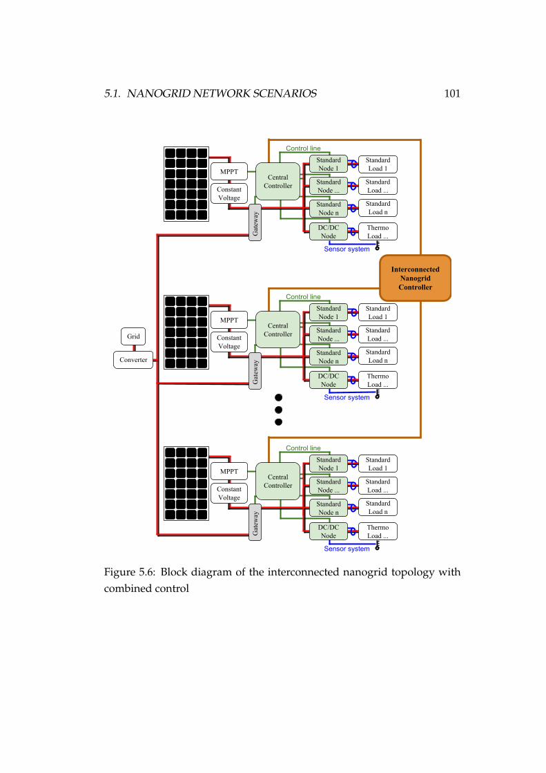
5.1. NANOGRID NETWORK SCENARIOS 101
Grid
Converter
Interconnected Nanogrid Controller
Constant Voltage
MPPTCentral
Controller
Standard Load 1
StandardLoad ...
StandardLoad n
Gat
eway
ThermoLoad ...
StandardNode 1
StandardNode ...
StandardNode n
DC/DCNode
Control line
Sensor system
Constant Voltage
MPPTCentral
Controller
Standard Load 1
StandardLoad ...
StandardLoad n
Gat
eway
ThermoLoad ...
StandardNode 1
StandardNode ...
StandardNode n
DC/DCNode
Control line
Sensor system
Constant Voltage
MPPTCentral
Controller
Standard Load 1
StandardLoad ...
StandardLoad n
Gat
eway
ThermoLoad ...
StandardNode 1
StandardNode ...
StandardNode n
DC/DCNode
Control line
Sensor system
Figure 5.6: Block diagram of the interconnected nanogrid topology withcombined control

102 CHAPTER 5. INTERCONNECTED NANOGRID NETWORK
In order to create a nanogrid network control strategy, the equationsgiven in chapter 4 need to be generalised to accommodate any numberof interconnected houses, each with thermostatically controlled loads. Toimplement combined control law, the duty cycle calculated for each ther-mostatically controlled load must consider all other loads and suppliesoperating in the network.
Equation (5.1) shows the maximum power point tracking supply sig-nal for the nanogrid network. It is a summation of all the available PVpower within the nanogrid network. Just as the nanogrid’s loadline canbe diverse, so can the PV capacity of each house.
PMPPTmicro= PInmicro
=
j∑i=1
VIniIIni
(5.1)
Where “j” is the number of interconnected nanogrids, PInmicrois the PV
power produced by each house while VIniand IIni
refer to the voltage andcurrent produced by each house respectively.
The power delivered to each of the nanogrid network’s thermostati-cally controlled loads by the control law must also be calculated. Equa-tions (5.2) through (5.5) show how the duty cycle (D) is calculated, as afunction of current (IIn, Io), for the buck converter present in the thermo-statically controlled load’s node. It considers the efficiency of the buckconverter (E ), output/input power (Po and PIn respectively), and out-put/input voltage (Vo and VIn respectively).
Vo = DVIn (5.2)
Po = EPIn (5.3)
DVInIo = E VInIIn (5.4)

5.1. NANOGRID NETWORK SCENARIOS 103
D =E VInIInVInIo
=E IInIo
(5.5)
Equations (5.6) and (5.7) consider the new variable PMPPTmicroand also
introduce VInmicro, a summation of the voltages (VIni
) produced by thecombined PV installations. This is used to derive the current producedby the interconnected nanogrid network (IInmicro
). The duty cycle deter-mining the output voltage of a thermostatically controlled load’s controlnode can then become a function of the power generated by the nanogridnetwork (5.8).
VInmicro=
∑ji=1 VIni
j(5.6)
IInmicro=PMPPTmicro
VInmicro
(5.7)
D =EPMPPTmicro
IoVInmicro
(5.8)
Although equation (5.8) gives the duty cycle for the control node, itdoes not consider other loads operating within the nanogrid network. Theduty cycle will need to be adjusted to consider the uncontrolled and ther-mostatically controlled loads operating in the network.
To do so, equation (5.9) is used to calculate the consumption of all un-controlled loads consuming power within the nanogrid network. Theseare loads that the consumer controls and expects an output when they areswitched on. Such loads are not controlled within the nanogrid to ensurethe comfort of the user.
Ltotalmicro=
n∑m=1
Ltotalm (5.9)
Where n is the number of loads operating, that are not thermostaticallycontrolled.

104 CHAPTER 5. INTERCONNECTED NANOGRID NETWORK
Next the measure of urgency of each thermostatically controlled loadneeds to be calculated. Equation (5.10) is used to calculate an estimated“on” period for each thermostatically controlled load, based on its currenttemperature, usage and thermal characteristics. The premise of this calcu-lation is that the load that will consume the largest amount of power fora particular time period (day) is the most urgent and needs to be servicedby PV power. The variable x relates to a load being powered while x1 isused if a load is not drawing power. For the water heater, equations (5.11)and (5.12) are used and the space heater, equations (5.13) and (5.14) (vari-ables for water and storage heater equations explained in tables 5.1 and5.2 respectively).
uT = Plog(x)
log(x) + log(x1)/day (5.10)
for water heater:
x =k
TW − mcTi+hATa+qmc+hA
(5.11)
where k is the constant of integration.
x1 =k1
TW − mcTi+hATa
mc+hA
(5.12)
where k1 is the constant of integration.
for space heater:x =
w
Tb − p(5.13)
where p =QIn + (a+ b+ c)TR
a+ b+ c, a =
kfbAfb
lfbMbcb, b =
ksAs
lsMbcb, c =
kvnAvn
Mbcband w
is the constant of integration
x1 =w1
Tb − TR(5.14)
where w1 is the constant of integration.

5.1. NANOGRID NETWORK SCENARIOS 105
Table 5.1: Explanation of variables in Eqn. (5.11) and (5.12)
Variable Descriptionc Specific heat of the water (J/kgC)m Flow rate (kg/h)TW Temperature of the water in the tank (C)Ti Temperature of the water entering the tank (C)h Heat transfer coefficient (for convection to ambient) (W/m2C)A Area of the tank (m2)Ta Ambient temperature (C)q Heat rate of the heating element (W )
Table 5.2: Explanation of variables in Eqn. (5.13) and (5.14)
Variable DescriptionMb Mass of the bricks (kg)cb Specific heat of the bricks (J/kgC)Tb Temperature of the bricks (C)TR Temperature of the room (C)QIn Input power (W )kfb Thermal conductivity of front and back (W/mC)Afb Area of the front and back (m2)lfb Thickness of the front and back (m)ks Thermal conductivity of the sides/top/bottom (W/mC)As Area of the sides/top/bottom (m2)ls Thickness of the sides/top/bottom (m)kvn Natural convection heat transfer coefficient (W/m2C)Avn Heat transfer area of the surface (m2)
The measure of urgency is then converted to a ratio as shown in equa-tion (5.15). This creates a hierarchy of the most to least urgent loads andgives a scaling factor for the duty cycle which is calculated in equation

106 CHAPTER 5. INTERCONNECTED NANOGRID NETWORK
(5.16). This duty cycle is the signal given to a control node (controllingload y) by the central controller, ensuring the load receives the ratio ofavailable PV power that is allocated.
This means, within the nanogrid network, the loads that are likely todraw the largest quantity of power over a given period of time (day), willbe serviced with the majority of the available PV power. It stands to reasonthat as a load receives power, heating its thermal mass, its measure ofurgency descends until another load becomes more urgent and is turnedon.
mmicroy =z∑
y=1
uTy∑zw=1 uTw
(5.15)
Where z is the number of thermostatically controlled loads within the clus-ter of houses
Dratioy = mmicroy
E (PMPPTmicro− Ltotalmicro
)
IoyVInmicro
(5.16)
Figure 5.7 shows the power consumption of a three house network anddisplays the ratio of power consumed by each water and storage heaterwithin the cluster. It also shows the total consumption which closely mir-rors the available PV power.
The safety measures discussed in chapter 4 remain active in the net-work and override control law. These are as follows, with in-depth expla-nations given in chapter 4:
• Water Lower Temperature Threshold: The water heater will be switchedon, regardless of PV power availability, if a lower temperature thresh-old is reached.
• Room Temperature: Rooms will be kept at a specific temperature re-gardless of PV power availability.
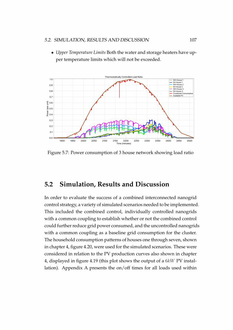
5.2. SIMULATION, RESULTS AND DISCUSSION 107
• Upper Temperature Limits Both the water and storage heaters have up-per temperature limits which will not be exceeded.
ThermostaticallyControlledLoadRatio
Time(minutes)1900 1950 2000 2050 2100 2150 2200 2250 2300 2350 2400 2450 2500
Power(perunit)
0.0
0.1
0.2
0.3
0.4
0.5
0.6
0.7
0.8
0.9
1.0 WHHouse1SHHouse1WHHouse2SHHouse2WHHouse3SHHouse3CombinedConsumptionAvailablePV
Figure 5.7: Power consumption of 3 house network showing load ratio
5.2 Simulation, Results and Discussion
In order to evaluate the success of a combined interconnected nanogridcontrol strategy, a variety of simulated scenarios needed to be implemented.This included the combined control, individually controlled nanogridswith a common coupling to establish whether or not the combined controlcould further reduce grid power consumed, and the uncontrolled nanogridswith a common coupling as a baseline grid consumption for the cluster.The household consumption patterns of houses one through seven, shownin chapter 4, figure 4.20, were used for the simulated scenarios. These wereconsidered in relation to the PV production curves also shown in chapter4, displayed in figure 4.19 (this plot shows the output of a 6kW PV instal-lation). Appendix A presents the on/off times for all loads used within

108 CHAPTER 5. INTERCONNECTED NANOGRID NETWORK
the 10 houses, along with refrigerator parameters, shower times/lengthsand hot water cylinder characteristics.
In order to show a correlation between the number of houses connectedand a reduction in grid power consumed, each of the three scenarios (com-bine control, individual control and uncontrolled) were simulated withtwo houses connected, increasing the number of interconnected houses byone each iteration of the simulation, until seven houses were reached (atwhich point the correlation was adequately established and the simula-tions became too large to continue).
The results of these simulations are shown in figures 5.8, 5.9, 5.10, andin tables 5.3 and 5.4. Figures 5.8 and 5.9 show the collective grid consump-tion of each scenario as the number of houses within the cluster increases.Fig 5.8 displays the summer scenario where it can be seen that the un-controlled consumption is the largest, and as the number of houses in thecluster increases, so to does the deviation between the combined and in-dividually controlled nanogrid networks (with the combined control con-suming less grid power than the individual).
A similar trend can be seen in 5.9 (winter consumption) between theuncontrolled and two controlled nanogrid networks. However, the com-bined and individually control nanogrid networks are much closer matched.This is due to the reduction in solar irradiance during the winter (com-pared to summer) and an increase in consumption due to regular use ofthe storage heater. In this situation, where the consumption heavily out-weighs the production, the system can do little to further improve thecluster’s ability to intelligently distribute the available PV power. Boththe individual and combined control schemes use all available PV.
Figure 5.10 shows a direct comparison between the individual andcombined control scenarios to quantify the magnitude to which the com-bined control has reduced the grid power consumption of the cluster (whencompared to the individual control). The plot displays, as a percentage,this reduction for the summer, winter, and yearly grid consumption. It

5.2. SIMULATION, RESULTS AND DISCUSSION 109
can be seen that the largest yearly reduction is approximately 7%, whichis achieved with 5 houses connected.
Tables 5.3 and 5.4 display the consumption of each scenario modelledin numerical format (for clarity), giving a kWh/day context.
Number of houses2 3 4 5 6 7
Grid
pow
er c
onsu
med
(W)
400
600
800
1000
1200
1400
1600
1800
2000Interconnected Nanogrid Grid Power Consumption(Summer)
Individual controlCombined controlUncontrolled
Figure 5.8: Summer consumption of 2 to 7 house clusters (Uncontrolled,individually controlled and combined control)
While comparisons have been made between three interconnected nanogridsolutions, it is also of interest to compare the network with the consump-tion of unconnected households. In figure 5.11, the accumulative con-sumption (2 to 7 houses) of the individually grid tied uncontrolled house-holds are compared to the interconnected nanogrid network’s combined

110 CHAPTER 5. INTERCONNECTED NANOGRID NETWORK
Number of houses2 3 4 5 6 7
Grid
pow
er c
onsu
med
(W)
0
1000
2000
3000
4000
5000
6000Interconnected Nanogrid Grid Power Consumption (Winter)
Individual controlCombined controlUncontrolled
Figure 5.9: Winter consumption of 2 to 7 house clusters (Uncontrolled,individually controlled and combined control)
control solution. It shows that increasing the number of households inthe network reduces the grid power consumption of the cluster, with twohouseholds yielding a 45% reduction and seven households, the largestreduction, delivering 61%.
5.2.1 The Effect of Varied PV Capacities
As discussed above, the PV capacity in the winter is often not sufficientto meet the loads operating in various households, reducing the effective-ness of the control strategy. To demonstrate this point, the five household

5.2. SIMULATION, RESULTS AND DISCUSSION 111
Number of Houses2 3 4 5 6 7
Red
uctio
n in
grid
pow
er re
duce
d (%
)
0
1
2
3
4
5
6
7
8
9Interconnected Nanogrid Reduction in Grid Power Consumption
SummerWinterYear
Redu
c&on
ingrid
pow
er(%
)
Figure 5.10: Reduction in grid power consumed by 2 to 7 house clusters(Uncontrolled, individually controlled and combined control)
uncontrolled and combined control scenarios were simulated with a va-riety of PV capacities (1kW , 2kW , 3kW , 6kW , 8kW and 10kW ). Figure5.12 shows the reduction in grid power consumed when the combinedcontrol interconnected nanogrid network is compared to the uncontrolledinterconnected nanogrid network scenario. It can be observed that the re-duction in grid power consumed increases with the increase in PV capac-ity. With the largest PV capacity installed (10kW ), the reduction is 58%. Asmentioned above, the three standard test scenario simulated in this sectionhad a PV installation of 6kW . Comparing the 6kW PV installation with the

112 CHAPTER 5. INTERCONNECTED NANOGRID NETWORK
Table 5.3: Comparison of power purchased by a cluster of households,with increasing size, in Wellington, NZ during Winter
Number ofhouses in cluster
UncontrolledkWh/day
Individual ControlkWh/day
Combined ControlkWh/day
2 36.23 20.77 20.333 55.43 29.84 29.634 70.11 32.03 31.095 94.82 46.91 44.226 120.45 55.74 55.617 140.35 64.25 62.14
Number of houses2 3 4 5 6 7R
educ
tion
in g
rid p
ower
con
sum
ed (%
)
40
45
50
55
60
65Uncontrolled Individual Houses Compared to Combined Control
Figure 5.11: Reduction in grid power consumed by uncontrolled, individ-ual houses when compared to combined control connected houses
10kW shown in figure 5.12, a further 6% reduction can be achieved.
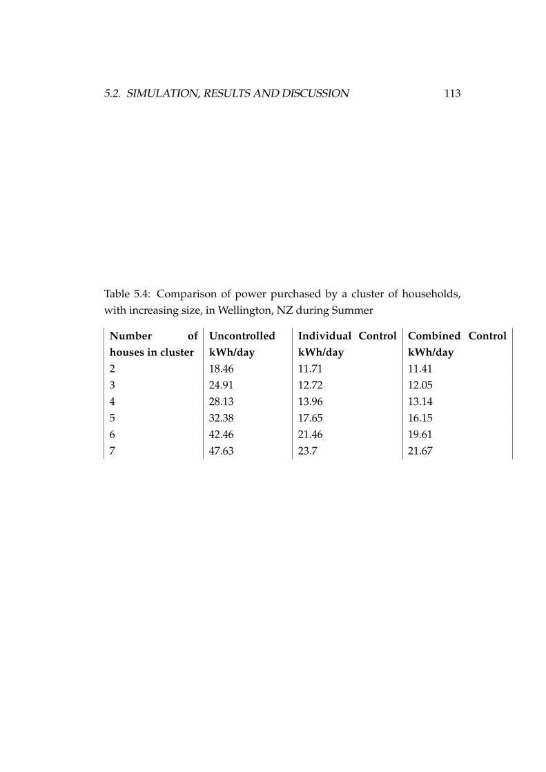
5.2. SIMULATION, RESULTS AND DISCUSSION 113
Table 5.4: Comparison of power purchased by a cluster of households,with increasing size, in Wellington, NZ during Summer
Number ofhouses in cluster
UncontrolledkWh/day
Individual ControlkWh/day
Combined ControlkWh/day
2 18.46 11.71 11.413 24.91 12.72 12.054 28.13 13.96 13.145 32.38 17.65 16.156 42.46 21.46 19.617 47.63 23.7 21.67

114 CHAPTER 5. INTERCONNECTED NANOGRID NETWORK
Household PV capacity (kW)1 2 3 4 5 6 7 8 9 10
Red
uctio
n in
Grid
Pow
er (%
)
30
35
40
45
50
55
60Reduction in Grid Power Purchased (5 house scenario)
Figure 5.12: Reduction in grid power consumed by 5 house clusters withvaried PV capacities (Uncontrolled and combined control)

5.3. CHAPTER SUMMARY 115
5.3 Chapter Summary
In this chapter, a novel control system is presented with the objective ofcreating a hierarchical power system that ensures the efficient use of lo-cally produced PV power within a small cluster of houses. The thermostat-ically controlled loads within the interconnected nanogrid network are notonly shifted, but modulated to increase the correlation between the powerconsumption and local PV production.
The maximum power point tracking signal is used to observe the avail-ability of local PV power. From this variable, an algorithm is produced tocontrol the duty cycle of a buck converter, which alters the voltage sup-plied to the thermostatically controlled loads. This algorithm not onlyconsiders local PV production, but the consumption of the loads that arenot TCL.
The algorithm then considers the expected consumption of each of theTCLs within the cluster of houses, creating a ratio variable which delegatesthe appropriate power to each of the TCLs. This ensures the loads that willconsume the most power over the day are serviced with the largest ratioof power, while the less urgent loads only consume a small amount ofpower. As the urgent loads receive the majority of the power, they drop inurgency, eventually becoming the less urgent loads within the cluster.
The combined control is simulated under a number of conditions (aweek summer and a week winter), with clusters ranging from 2 housesto 7. The total grid power consumed by the combined control system isthen compared to the grid power consumed by a cluster of uncontrolledhouses, and a cluster of individually controlled houses. The results showthat the combined control scenario can improve on the uncontrolled clus-ters by as much as 55%, while the improvement when compared to theindividually control nanogrid cluster is as much as 7%.
If the combined nanogrid network controller is compared to uncon-trolled houses, not in a cluster, the reduction in grid power consumed is

116 CHAPTER 5. INTERCONNECTED NANOGRID NETWORK
as much as 61%.

Chapter 6
Conclusions and Future Work
The centralised power grid is an amazing feat of interdisciplinary engi-neering, capable of supplying power to millions of households globally.But with a system of this magnitude there are often new challenges, un-foreseen consequences and room for improvement. In the case of cen-tralised power generation, the challenges involve environmental impact(carbon emissions), efficiency (line losses) and robustness (susceptibilityto outages due to long distance transmission).
Distributed generation, in the form of small-scale renewable energy,has the potential to negate these issues, offering a clean energy source andlocalised generation. However, small-scale renewable energy is not with-out fault, presenting the challenge of an intermittent power source. Inter-mittency, in the case of PV, refers to a mismatch of high power productiontimes with a household’s high consumption time. This essentially leavesa large amount of unused PV power (which can be sold to the grid butbuyback prices are often low) and a household which still needs to pur-chase the majority of its power from the national grid. This is a situationwhich needs to be overcome in order to see the acceptance of small-scalePV systems as a viable option for individuals and users within small com-munities.
The research presented in this thesis addresses intermittency through
117

118 CHAPTER 6. CONCLUSIONS AND FUTURE WORK
the use of a nanogrid (a controlled power distribution system for a singlehousehold) which utilises thermostatically controlled loads to increase thecorrelation between a household’s power consumption and production. Itthen investigates the impact connecting multiple nanogrids, forming aninterconnected nanogrid network, can have to further reduce the effects ofintermittency for a small community.
Research into the use of nanogrids, thermostatically controlled loadsand interconnected nanogrid networks is represented in literature, cre-ating a strong knowledge base of successful implementation and poten-tial for improvement. While nanogrid control and hardware are readilydiscussed, the definition of the nanogrid itself is vague and varies. Thenanogrid control literature focuses heavily on supply side managementfor stability, efficiency and grid regulation. However, it neglects to inves-tigate the use of demand side management to motivate the uptake of PVsystems and using the PV’s maximum power point tracker to implementDSM.
The research presented in the literature surrounding thermostaticallycontrolled loads is typically focused on pursuing goals set out by grid util-ity companies such as grid stabilisation and peak power reduction. Someresearch in the field of household control exists, however, the research failsto offer independent control strategies, utilising multiple thermostaticallycontrolled loads.
Interconnected nanogrid network research is a relatively new topic,where the majority of the literature presented is conceptual. While somework has delved into supply side management, demand side managementcontrol strategies, specifically strategies that consider all nanogrids withinthe larger entity forming a cohesive control structure, is not yet presentedwithin the literature.
It is clear to see, from the gaps in the literature, that research intonanogrids and interconnected nanogrids can be progressed in the area ofdemand side management through the use of thermostatically controlled

119
loads, to incentivise PV installations at a household level.
To achieve this ambitious task, three objectives were set; The first, todefine the nanogrid structure so it could be discussed as a stand alonepower system. The second, to create a nanogrid control strategy that willincrease the correlation between power consumption and production, util-ising thermostatically controlled loads. And lastly, to expand the controlstrategy to facilitate an interconnected nanogrid network which will al-low the sharing of power within a cluster of houses. A summary of theimplementation and the extent to which the goals were achieved follows:
1. In order to define the nanogrid structure, the various characteristicsused within the literature to describe a nanogrid were collated. Theadvantages and disadvantages of each were presented and analysedwith the goal of reducing ambiguity around the power structure.From this, the key defining factors were used to create the follow-ing concise definition:”A nanogrid is a power distribution system for a single house/small build-ing, with the ability to connect or disconnect from other power entities viaa gateway. It consists of local power production powering local loads, withthe option of utilising energy storage and/or a control system.”
2. To create a nanogrid controller that increased the correlation betweenPV power production and household consumption, two initial itemsof knowledge were required: The available PV power at any partic-ular time and household loads that could be shifted without causingdiscomfort to the residents. To obtain knowledge of the availablePV power, the novel approach of using the maximum power pointtracking signal was derived. Meaning that regardless of the load’sbehaviour, the control system could obtain PV production data, mak-ing it ideal for the purpose. Thermostatically controlled loads, specif-ically the water heater, storage heater and refrigerator, were selectedto implement the shifting of a household’s consumption. Due to

120 CHAPTER 6. CONCLUSIONS AND FUTURE WORK
their slow thermal dynamics, large power consumption and abil-ity to store energy in the form of heat, they presented a large por-tion of daily consumption that could be shifted with no discomfortto the households residents. With these variables in place, a con-trol strategy was developed that delegated a percentage of the avail-able PV power, after standard household loads were accounted for,to water and storage heater. This ratio was based on the expectedpower draw of either load over a day, with the load requiring themost power receiving a higher ratio. As these loads were resistivein nature, by altering the voltage at their input, it allowed the powerto be modulated to achieve this control strategy. The refrigeratoralso contributed to DSM with a separate algorithm that minimisedits consumption outside of PV production times. To test the algo-rithm, ten households were simulated with a variety of consumptioncurves that considered the diversity observed in summer and win-ter. The solar irradiance for a week in summer and winter (Kelburn,Wellington, New Zealand) was also obtained to achieve a realistictest scenario. The scenarios were simulated under two conditions,controlled and uncontrolled, in order to quantify the nanogrid’s abil-ity to reduce grid power consumed. It was found that the system hadthe ability to reduce the grid power consumed by as much as 61.86%,with a minimum reduction of 22.38%. The average reduction acrossall test scenarios was 44.28%.
3. While the single household nanogrid achieved a remarkable reduc-tion in grid power consumed, the pursuit of further grid power re-duction led to the investigation of interconnected nanogrid networks.The concept stems from the diversity in consumption and produc-tion that occurs within a community. To utilise this characteristic, aninterconnected nanogrid network control strategy was developed.The control strategy was made up of the maximum power pointtracking signal within each house, collating the combined produc-

121
tion. It then observed the consumption of all uncontrollable loadswithin the network. With this information, an algorithm, which con-sidered all thermostatically controlled loads within the cluster of houses,was implemented. A percentage of the available PV power wasdelegated to each thermostatically controlled load based on its “ur-gency”, ie a measure of which load was likely to draw the mostpower over a specific period (day). The loads with the largest powerdraw were served with the majority of available PV power, whilethe loads with the lower power draw, a lesser percentage. As eachload was serviced, by default its “urgency” would decrease, ensur-ing the loads that initially presented a low “urgency” would in turnbecome the more urgent and receive a higher ratio of power. In or-der to quantify the success of the solution, three simulated scenarioswere established. The first was an uncontrolled network, the seconda network of nanogrids with individual control and the last, a com-bined control strategy. The size of the cluster was increased from twoto seven interconnected households, with varied consumption pat-terns and summer/winter conditions (Higher consumption in win-ter and each season having the appropriate weekly solar irradiancedata for Kelburn, Wellington, New Zealand). The grid consumptionof each scenario, over a simulated week, was monitored and com-pared. The first insight showed that, compared to individually gridconnected houses, even the uncontrolled network displayed a reduc-tion in grid consumption. The results also showed that the combinedcontrol, when compared to the uncontrolled cluster, had the abilityto reduce grid power consumed by as much as 55%, the minimumbeing 42% (two houses). When compared to the individually con-trolled nanogrids, the results were much closer with a maximum re-duction of 7% and a minimum of 2%. This comparison was made as-suming an identical PV consumption curve, but as discussed in thefuture work, the combined control strategy could present a much

122 CHAPTER 6. CONCLUSIONS AND FUTURE WORK
higher reduction in grid power consumed (when compared to theindividually controlled nanogrids) given varied PV curves (due totopographical variations for example). For completeness, a compar-ison was also made between the combined control and individuallygrid connected uncontrolled houses. It was found that the combinedcontrol strategy can reduce the grid power consumed by as much as61% in this case.
The achievement of the research objectives leads to the major researchcontributions of this thesis:
Major research contributions
1. This thesis presents a rigorous analysis of the general nanogrid defi-nitions given within the literature, discussing their merits and weak-nesses from which a concise definition of a nanogrid structure is de-rived. The traditional supply side management control structuresare presented and extended to include demand side management.A new control structure which improves the hybrid central controlstrategy is also presented.
2. This thesis develops a novel nanogrid control scheme that makesuse of thermostatically controlled loads to address intermittency ofphotovoltaic (PV) modules, negating the need for traditional storageand enabling the user to reduce grid power consumed. This strategyshifts away from direct or indirect control signals received from theutilities and introduces the concept of using a maximum power pointtracking signal to instantaneously shift electricity consumption, dy-namically matching local PV production. Simulated under a varietyof load and solar irradiance conditions, the nanogrid control schemeshows the ability to reduce grid power consumed by 44%.
3. This thesis presents a control scheme that facilitates the interconnec-tion of multiple nanogrids. This scheme extends the capabilities of

6.1. FUTURE WORK 123
the single nanogrid control to dynamically match the consumptionand production of a cluster of interconnected households. This con-trol scheme further reduces the effect of intermittency, taking ad-vantage of diversity of consumption within a cluster of houses. Acomparison of grid power consumed by the cluster of houses is pre-sented, considering uncontrolled, individually controlled and thecombined control scenarios. The simulated tests show that, com-pared to an uncontrolled nanogrid network, the combined controlcan reduce grid power consumed by as much as 55%, while a 7%decrease is seen when comparing the combined control with the in-dividually controlled nangrid networks. When compared to an un-controlled individual house scenario, the combined control intercon-nected nanogrids can reduce the power purchase from the grid by asmuch as 61%.
This thesis has proven that increasing the correlation between PV powerproduced and a household’s power consumption, through the use of DSM,reduces the negative effects of intermittency and ultimately a household’sgrid consumption. This increases the viability of small scale PV systemsat a residential level, which encourages the uptake of carbon neutral, dis-tributed energy.
6.1 Future Work
During the course of this research, a number of topics presented them-selves as opportunities to further this work. These are as follows:
• Practical implementation: The next logical step in this research wouldsee a physical implementation of the nanogrid and nanogrid net-work solutions. This would highlight any real world issues thatdid not present themselves in the simulated scenarios, an example isthe effect of electromagnetic interference (EMI) which has not been
124 CHAPTER 6. CONCLUSIONS AND FUTURE WORK
considered in the model. A nanogrid with the capability of operat-ing autonomously, controlled and uncontrolled, should be created.Long term observation of the power flows and environmental con-ditions should be monitored to enable real world comparisons be-tween the two solutions. A community of nanogrids should thenbe established, with the ability to implement combined control andfurther observations should be made.
• Financial analysis: Once the practical implementation has occurred,a financial analysis should be conducted. This would see a cost andlife cycle analysis of the control system’s central controller and con-trol nodes. The financial saving achieved by the reduction in gridpower consumed when the control system is active should be quan-tified. The ultimate goal of the financial analysis should be to dis-cover whether the control system increases the financial viability ofsmall scale PV systems at a household level.
• Nanogrid network varied solar irradiance patterns: While the so-lution presented in this research considers a single solar irradiancepattern for all houses within the nanogrid network, this may not al-ways be the case. Topographical variations, such as tree placement,valleys or hills might see households receive sun at different timesof day. This may be where a network approach to sharing powerbenefits occupants immensely. Take for example a cluster of house-holds situated half on one side of a valley, and half on the oppositeside. If morning sun is received by side “a”, and evening received byside “b”, “a” may supply “b” in the morning and vice versa in theevening. This is a situation that should be further explored with thethree nanogrid network solutions (uncontrolled, individually con-trolled and combined control).
• Cold storage devices: The storage heater is a key device in mak-ing this control system capable of consuming large amounts of PV

6.1. FUTURE WORK 125
power. This does work under the assumption that heating is re-quired, making it a system compatible with countries (eg New Zealand)with colder climates. In order to maximise the solution for countriescloser to the equator, where cooling is required, an equivalent to thestorage heater must be found that can be used to cool households.Ideally this solution will be resistive in nature, making air condi-tioning units less ideal. Exploration into the use of thermoelectricdevices could see the solution thrive in warmer climates, if the effi-ciency of these devices is improved.
• Communication systems: In both the nanogrid and nanogrid net-work, communication plays an important role in transactions be-tween the microgrid, central and node controllers. Future researchwould see a cohesive communications system implemented. As dis-cussed in chapter 3, PLCs could be pursed to create a robust systemthat negates the need for additional communications lines. Wire-less communication could also be possible if security and robustnesswere considered.
• Nanogrid network pricing scheme: As household PV installationsmay vary in size, leading to certain households in a cluster supply-ing more power, financial compensation should be considered. Thiswould be an algorithm written into the microgrid controller thatmonitors power flows in and out of each house in the cluster. Acost of power flowing within the network would be assigned thatwould be of mutual benefit to both seller and buyer, further moti-vating the cluster. The seller would receive more compensation thanthat offered by the grid (eg greater than the 10c/kWh offered in NewZealand) and the buyer would buy for less than offered by the grid(eg less than the 28c/kWh offered in New Zealand). The algorithmcould monitor the total power purchased by the cluster and ratherthan money being exchanged between occupants, it could calculate

126 CHAPTER 6. CONCLUSIONS AND FUTURE WORK
the ratio that each customer would need to pay towards the cluster’spower bill.

Bibliography
[1] S. Kalambe and G. Agnihotri, “Loss minimization techniques usedin distribution network: bibliographical survey,” Renewable and Sus-tainable Energy Reviews, vol. 29, pp. 184 – 200, 2014.
[2] A. M. Haidar, K. Muttaqi, and D. Sutanto, “Smart grid and its futureperspectives in australia,” Renewable and Sustainable Energy Reviews,vol. 51, pp. 1375 – 1389, 2015.
[3] S. Uski and I. Kim, “Assessment of wind power impact on powersystem transmission losses,” in IEEE PES Innovative Smart Grid Tech-nologies, Europe, pp. 1–5, Oct 2014.
[4] P. J. Maliszewski, E. K. Larson, and C. Perrings, “Environmentaldeterminants of unscheduled residential outages in the electricalpower distribution of phoenix, arizona,” Reliability Engineering andSystem Safety, vol. 99, pp. 161 – 171, 2012.
[5] A. Pahwa, “Effect of environmental factors on failure rate of over-head distribution feeders,” in IEEE Power Engineering Society GeneralMeeting, 2004., pp. 691–692 Vol.1, June 2004.
[6] P. Friedlingstein, R. Houghton, G. Marland, J. Hackler, T. A. Boden,T. Conway, J. Canadell, M. Raupach, P. Ciais, and C. Le Quere, “Up-date on co2 emissions,” Nature Geoscience, vol. 3, no. 12, pp. 811–812,2010.
127

128 BIBLIOGRAPHY
[7] D. Akinyele, R. Rayudu, and N. Nair, “Global progress in photo-voltaic technologies and the scenario of development of solar panelplant and module performance estimation application in nigeria,”Renewable and Sustainable Energy Reviews, vol. 48, pp. 112 – 139, 2015.
[8] D. Akinyele, R. Rayudu, and N. Nair, “Development of photovoltaicpower plant for remote residential applications: The socio-technicaland economic perspectives,” Applied Energy, vol. 155, pp. 131 – 149,2015.
[9] H. Holtorf, T. Urmee, M. Calais, and T. Pryor, “A model to evaluatethe success of solar home systems,” Renewable and Sustainable EnergyReviews, vol. 50, pp. 245 – 255, 2015.
[10] P. Basak, S. Chowdhury, S. H. nee Dey, and S. Chowdhury, “A litera-ture review on integration of distributed energy resources in the per-spective of control, protection and stability of microgrid,” Renewableand Sustainable Energy Reviews, vol. 16, no. 8, pp. 5545 – 5556, 2012.
[11] J. J. Justo, F. Mwasilu, J. Lee, and J.-W. Jung, “Ac-microgrids versusdc-microgrids with distributed energy resources: A review,” Renew-able and Sustainable Energy Reviews, vol. 24, pp. 387 – 405, 2013.
[12] C. Rae and F. Bradley, “Energy autonomy in sustainable communi-tiesa review of key issues,” Renewable and Sustainable Energy Reviews,vol. 16, no. 9, pp. 6497 – 6506, 2012.
[13] Y. Cao, X. Wang, Y. Li, Y. Tan, J. Xing, and R. Fan, “A comprehensivestudy on low-carbon impact of distributed generations on regionalpower grids: A case of jiangxi provincial power grid in china,” Re-newable and Sustainable Energy Reviews, vol. 53, pp. 766 – 778, 2016.
[14] P. Paliwal, N. Patidar, and R. Nema, “Planning of grid integrateddistributed generators: A review of technology, objectives and tech-

BIBLIOGRAPHY 129
niques,” Renewable and Sustainable Energy Reviews, vol. 40, pp. 557 –570, 2014.
[15] S. Sivarasu, E. C. Sekaran, and P. Karthik, “Development of renew-able energy based microgrid project implementations for residentialconsumers in india: Scope, challenges and possibilities,” Renewableand Sustainable Energy Reviews, vol. 50, pp. 256 – 269, 2015.
[16] P. Descateaux, M. F. Astudillo, and M. B. Amor, “Assessing the lifecycle environmental benefits of renewable distributed generation ina context of carbon taxes: The case of the northeastern americanmarket,” Renewable and Sustainable Energy Reviews, vol. 53, pp. 1178– 1189, 2016.
[17] F. F. Yanine and E. E. Sauma, “Review of grid-tie micro-generationsystems without energy storage: Towards a new approach to sus-tainable hybrid energy systems linked to energy efficiency,” Renew-able and Sustainable Energy Reviews, vol. 26, pp. 60 – 95, 2013.
[18] M. Y. Suberu, M. W. Mustafa, and N. Bashir, “Energy storage sys-tems for renewable energy power sector integration and mitigationof intermittency,” Renewable and Sustainable Energy Reviews, vol. 35,pp. 499 – 514, 2014.
[19] D. Akinyele and R. Rayudu, “Review of energy storage technologiesfor sustainable power networks,” Sustainable Energy Technologies andAssessments, vol. 8, pp. 74 – 91, 2014.
[20] P. Twomey and K. Neuhoff, “Wind power and market power in com-petitive markets,” Energy Policy, vol. 38, no. 7, pp. 3198 – 3210, 2010.Large-scale wind power in electricity markets with Regular Papers.
[21] E. K. Stigka, J. A. Paravantis, and G. K. Mihalakakou, “Social accep-tance of renewable energy sources: A review of contingent valua-
130 BIBLIOGRAPHY
tion applications,” Renewable and Sustainable Energy Reviews, vol. 32,pp. 100 – 106, 2014.
[22] S. J. Oliva and I. F. MacGill, “Estimating the economic value of dis-tributed pv systems in australia,” in Innovative Smart Grid Technolo-gies Asia (ISGT), 2011 IEEE PES, pp. 1–8, Nov 2011.
[23] Ministry of Business Innovation and Employment, “Sales-based electricity costs 2016.” http://www.mbie.govt.nz/info-services/sectors-industries/energy/energy-data-modelling/statistics/prices/electricity-prices/sales-based-residential-prices.pdf.
[24] A. Miller, M. Hwang, S. Lemon, E. G. Read, and A. Wood, “Eco-nomics of Photovoltaic Solar Power and Uptake in New Zealand,”EEA Conference and Exhibition, Wellington, 2015.
[25] J. Bryan, R. Duke, and S. Round, “Decentralized generator schedul-ing in a nanogrid using dc bus signaling,” in IEEE Power EngineeringSociety General Meeting, 2004., pp. 977–982 Vol.1, June 2004.
[26] J. Schonberger, R. Duke, and S. D. Round, “Dc-bus signaling: A dis-tributed control strategy for a hybrid renewable nanogrid,” IEEETransactions on Industrial Electronics, vol. 53, pp. 1453–1460, Oct 2006.
[27] R. P. S. Chandrasena, F. Shahnia, A. Ghosh, and S. Rajakaruna, “Op-eration and control of a hybrid ac-dc nanogrid for future communityhouses,” in 2014 Australasian Universities Power Engineering Confer-ence (AUPEC), pp. 1–6, Sept 2014.
[28] S. H. Latha and S. C. Mohan, “Centralized power control strategyfor 25 kw nano grid for rustic electrification,” in 2012 InternationalConference on Emerging Trends in Science, Engineering and Technology(INCOSET), pp. 456–461, Dec 2012.

BIBLIOGRAPHY 131
[29] D. Qu, M. Wang, Z. Sun, and G. Chen, “An improved dc-bus signal-ing control method in a distributed nanogrid interfacing modularconverters,” in 2015 IEEE 11th International Conference on Power Elec-tronics and Drive Systems, pp. 214–218, June 2015.
[30] W. Zhang, F. C. Lee, and P. Y. Huang, “Energy management systemcontrol and experiment for future home,” in 2014 IEEE Energy Con-version Congress and Exposition (ECCE), pp. 3317–3324, Sept 2014.
[31] A. Riccobono, M. Ferdowsi, J. Hu, H. Wolisz, P. Jahangiri, D. Mller,R. W. D. Doncker, and A. Monti, “Next generation automation archi-tecture for dc smart homes,” in 2016 IEEE International Energy Con-ference (ENERGYCON), pp. 1–6, April 2016.
[32] A. S. Morais and L. A. C. Lopes, “Interlink converters in dcnanogrids and its effect in power sharing using distributed control,”in 2016 IEEE 7th International Symposium on Power Electronics for Dis-tributed Generation Systems (PEDG), pp. 1–7, June 2016.
[33] A. Malkawi and L. A. C. Lopes, “Control of the power electron-ics interface of a pv source in a smart residential dc nanogrid,” in2016 IEEE Canadian Conference on Electrical and Computer Engineering(CCECE), pp. 1–4, May 2016.
[34] R. P. S. Chandrasena, F. Shahnia, S. Rajakaruna, and A. Ghosh, “Dy-namic operation and control of a hybrid nanogrid system for futurecommunity houses,” IET Generation, Transmission Distribution, vol. 9,no. 11, pp. 1168–1178, 2015.
[35] A. Brocco, “Fully distributed power routing for an ad hocnanogrid,” in 2013 IEEE International Workshop on Inteligent EnergySystems (IWIES), pp. 113–118, Nov 2013.
132 BIBLIOGRAPHY
[36] U. B. Mujumdar and D. R. Tutkane, “Parallel mppt for pv based res-idential dc nanogrid,” in International Conference on Industrial Instru-mentation and Control (ICIC), pp. 1350–1355, May 2015.
[37] J. Schonberger, S. Round, and R. Duke, “Autonomous load sheddingin a nanogrid using dc bus signalling,” in IECON 2006 - 32nd AnnualConference on IEEE Industrial Electronics, pp. 5155–5160, Nov 2006.
[38] P. Yi, X. Dong, A. Iwayemi, C. Zhou, and S. Li, “Real-time oppor-tunistic scheduling for residential demand response,” IEEE Transac-tions on Smart Grid, vol. 4, pp. 227–234, March 2013.
[39] M. Biabani, M. A. Golkar, A. Johar, and M. Johar, “Propose a homedemand-side-management algorithm for smart nano-grid,” in 4thAnnual International Power Electronics, Drive Systems and TechnologiesConference, pp. 487–494, Feb 2013.
[40] S. Barker, A. Mishra, D. Irwin, P. Shenoy, and J. Albrecht, “Smartcap:Flattening peak electricity demand in smart homes,” in 2012 IEEEInternational Conference on Pervasive Computing and Communications,pp. 67–75, March 2012.
[41] R. Adda, O. Ray, S. K. Mishra, and A. Joshi, “Synchronous-reference-frame-based control of switched boost inverter for stan-dalone dc nanogrid applications,” IEEE Transactions on Power Elec-tronics, vol. 28, pp. 1219–1233, March 2013.
[42] A. Goikoetxea, J. M. Canales, R. Sanchez, and P. Zumeta, “Dc versusac in residential buildings: Efficiency comparison,” in Eurocon 2013,pp. 1–5, July 2013.
[43] H. S. Kim, M. H. Ryu, J. W. Baek, and J. H. Jung, “High-efficiencyisolated bidirectional ac-dc converter for a dc distribution system,”IEEE Transactions on Power Electronics, vol. 28, pp. 1642–1654, April2013.

BIBLIOGRAPHY 133
[44] H. Mamur and R. Ahiska, “Application of a dcdc boost converterwith maximum power point tracking for low power thermoelectricgenerators,” Energy Conversion and Management, vol. 97, pp. 265 –272, 2015.
[45] D. Burmester, R. Rayudu, and T. Exley, “Single ended primary in-ductor converter reliance of efficiency on switching frequency foruse in mppt application,” in 2013 IEEE PES Asia-Pacific Power andEnergy Engineering Conference (APPEEC), pp. 1–6, Dec 2013.
[46] M. Taghvaee, M. Radzi, S. Moosavain, H. Hizam, and M. H. Marha-ban, “A current and future study on non-isolated dcdc convertersfor photovoltaic applications,” Renewable and Sustainable Energy Re-views, vol. 17, pp. 216 – 227, 2013.
[47] S. G. Tesfahunegn, P. J. S. Vie, . Ulleberg, and T. M. Undeland, “Asimplified battery charge controller for safety and increased utiliza-tion in standalone pv applications,” in 2011 37th IEEE PhotovoltaicSpecialists Conference, pp. 002441–002447, June 2011.
[48] R. Sarath and P. Kanakasabapathy, “Switched-capacitor/switched-inductor cuk-derived hybrid converter for nanogrid applications,”in 2015 International Conference on Computation of Power, Energy, In-formation and Communication (ICCPEIC), pp. 0430–0435, April 2015.
[49] S. Poshtkouhi, M. Fard, H. Hussein, L. M. D. Santos, O. Trescases,M. Varlan, and T. Lipan, “A dual-active-bridge based bi-directionalmicro-inverter with integrated short-term li-ion ultra-capacitor stor-age and active power smoothing for modular pv systems,” in 2014IEEE Applied Power Electronics Conference and Exposition - APEC 2014,pp. 643–649, March 2014.
[50] O. Ray and S. Mishra, “A multi-port converter topology with simul-taneous isolated and non-isolated outputs,” in IECON 2013 - 39th

134 BIBLIOGRAPHY
Annual Conference of the IEEE Industrial Electronics Society, pp. 7118–7123, Nov 2013.
[51] O. Ray and S. Mishra, “Boost-derived hybrid converter with simul-taneous dc and ac outputs,” IEEE Transactions on Industry Applica-tions, vol. 50, pp. 1082–1093, March 2014.
[52] S. Poshtkouhi and O. Trescases, “Multi-input single-inductor dc-dcconverter for mppt in parallel-connected photovoltaic applications,”in 2011 Twenty-Sixth Annual IEEE Applied Power Electronics Conferenceand Exposition (APEC), pp. 41–47, March 2011.
[53] M. C. Mira, Z. Zhang, A. Knott, and M. A. E. Andersen, “Powerflow control of a dual-input interleaved buck/boost converter withgalvanic isolation for renewable energy systems,” in 2015 IEEE Ap-plied Power Electronics Conference and Exposition (APEC), pp. 3007–3012, March 2015.
[54] H. Keyhani and H. A. Toliyat, “Single-stage multistring pv inverterwith an isolated high-frequency link and soft-switching operation,”IEEE Transactions on Power Electronics, vol. 29, pp. 3919–3929, Aug2014.
[55] A. S. U., S. S. Nag, and S. K. Mishra, “A multi-input single-control(misc) battery charger for dc nanogrids,” in 2013 IEEE ECCE AsiaDownunder, pp. 304–310, June 2013.
[56] F. Chen, R. Burgos, D. Boroyevich, and D. Dong, “Control loop de-sign of a two-stage bidirectional ac/dc converter for renewable en-ergy systems,” in 2014 IEEE Applied Power Electronics Conference andExposition - APEC 2014, pp. 2177–2183, March 2014.
[57] D. Dong, F. Luo, X. Zhang, D. Boroyevich, and P. Mattavelli, “Grid-interface bidirectional converter for residential dc distribution sys-tems; part 2: Ac and dc interface design with passive compo-

BIBLIOGRAPHY 135
nents minimization,” IEEE Transactions on Power Electronics, vol. 28,pp. 1667–1679, April 2013.
[58] D. Dong, I. Cvetkovic, D. Boroyevich, W. Zhang, R. Wang, andP. Mattavelli, “Grid-interface bidirectional converter for residentialdc distribution systems; part one: High-density two-stage topol-ogy,” IEEE Transactions on Power Electronics, vol. 28, pp. 1655–1666,April 2013.
[59] S. S. Nag and S. Mishra, “Current-fed dc/dc topology based in-verter,” in 2013 IEEE Energy Conversion Congress and Exposition,pp. 2751–2756, Sept 2013.
[60] S. S. Nag, R. Adda, O. Ray, and S. K. Mishra, “Current-fed switchedinverter based hybrid topology for dc nanogrid application,” inIECON 2013 - 39th Annual Conference of the IEEE Industrial ElectronicsSociety, pp. 7146–7151, Nov 2013.
[61] R. Adda, O. Ray, S. Mishra, and A. Joshi, “Dsp based pwm controlof switched boost inverter for dc nanogrid applications,” in IECON2012 - 38th Annual Conference on IEEE Industrial Electronics Society,pp. 5285–5290, Oct 2012.
[62] A. Tomy and A. J. Thomas, “Sepic derived hybrid converter with si-multaneous ac and dc outputs,” in 2016 IEEE Annual India Conference(INDICON), pp. 1–6, Dec 2016.
[63] O. D. Castle and A. E. Shahat, “Single-input - multi-output (simo)converter for nano-grids applications,” in SoutheastCon 2017, pp. 1–5, March 2017.
[64] N. Isaacs, M. Camilleri, L. Burrough, K. Saville-smith, and R. F.Cresa, “Energy Use in New Zealand Households Final Report onthe Household Energy End-use PRoject (HEEP),” Science And Tech-nology, vol. 221, 2010.

136 BIBLIOGRAPHY
[65] N. Lu, P. Du, and Y. V. Makarov, “The potential of thermostaticallycontrolled appliances for intra-hour energy storage applications,” in2012 IEEE Power and Energy Society General Meeting, pp. 1–6, July2012.
[66] Z. Chen, L. Wu, and Y. Fu, “Real-time price-based demand responsemanagement for residential appliances via stochastic optimizationand robust optimization,” IEEE Transactions on Smart Grid, vol. 3,pp. 1822–1831, Dec 2012.
[67] E. C. Kara, M. Berges, B. Krogh, and S. Kar, “Using smart devicesfor system-level management and control in the smart grid: A re-inforcement learning framework,” in 2012 IEEE Third InternationalConference on Smart Grid Communications (SmartGridComm), pp. 85–90, Nov 2012.
[68] N. Lu, “An evaluation of the hvac load potential for providing loadbalancing service,” IEEE Transactions on Smart Grid, vol. 3, pp. 1263–1270, Sept 2012.
[69] Y. Zhang and N. Lu, “Parameter selection for a centralized thermo-statically controlled appliances load controller used for intra-hourload balancing,” IEEE Transactions on Smart Grid, vol. 4, pp. 2100–2108, Dec 2013.
[70] M. Alizadeh and A. Scaglione, “Least laxity first scheduling of ther-mostatically controlled loads for regulation services,” in 2013 IEEEGlobal Conference on Signal and Information Processing, pp. 503–506,Dec 2013.
[71] E. C. Kara, Z. Kolter, M. Berges, B. Krogh, G. Hug, and T. Yuksel,“A moving horizon state estimator in the control of thermostaticallycontrolled loads for demand response,” in 2013 IEEE International

BIBLIOGRAPHY 137
Conference on Smart Grid Communications (SmartGridComm), pp. 253–258, Oct 2013.
[72] E. Vrettos and G. Andersson, “Combined load frequency control andactive distribution network management with thermostatically con-trolled loads,” in 2013 IEEE International Conference on Smart GridCommunications (SmartGridComm), pp. 247–252, Oct 2013.
[73] M. A. Zehir, A. Batman, and M. Bagriyanik, “An event-drivenenergy management system for planned control of thermostaticloads,” in 2013 IEEE Grenoble Conference, pp. 1–6, June 2013.
[74] H. T. Nguyen, D. Nguyen, and L. B. Le, “Home energy manage-ment with generic thermal dynamics and user temperature prefer-ence,” in IEEE International Conference on Smart Grid Communications(SmartGridComm), pp. 552–557, Oct 2013.
[75] A. Abiri-Jahromi and F. Bouffard, “Characterizing statistical boundson aggregated demand-based primary frequency control,” in 2013IEEE Power Energy Society General Meeting, pp. 1–5, July 2013.
[76] Y. Zhang and N. Lu, “Demand-side management of air conditioningcooling loads for intra-hour load balancing,” in 2013 IEEE PES Inno-vative Smart Grid Technologies Conference (ISGT), pp. 1–6, Feb 2013.
[77] N. Lu, “Design considerations of a centralized load controller usingthermostatically controlled appliances for continuous regulation re-serves,” in 2013 IEEE Power Energy Society General Meeting, pp. 1–1,July 2013.
[78] H. Wang, K. Meng, F. Luo, Z. Y. Dong, Z. Xu, and K. P. Wong, “A hi-erarchical optimization framework for aggregating thermostaticallycontrolled loads to minimize real-time thermal rating of overheaddistribution lines,” in 2014 China International Conference on Electric-ity Distribution (CICED), pp. 1769–1773, Sept 2014.

138 BIBLIOGRAPHY
[79] A. K. Marinov, G. Verbi?, and A. C. Chapman, “An investigation intothe economic benefits of fast-timescale demand response using ther-mostatically controlled loads on the nem,” in 2014 Australasian Uni-versities Power Engineering Conference (AUPEC), pp. 1–6, Sept 2014.
[80] C. Vivekananthan, Y. Mishra, and K. Rajashekara, “Energy effi-cient home with price sensitive stochastically programmable TCAs,”in 40th Annual Conference of the IEEE Industrial Electronics Society,pp. 5357–5362, Oct 2014.
[81] M. Vanouni and N. Lu, “Improving the centralized control of ther-mostatically controlled appliances by obtaining the right informa-tion,” IEEE Transactions on Smart Grid, vol. 6, pp. 946–948, March2015.
[82] S. Grammatico, B. Gentile, F. Parise, and J. Lygeros, “A mean fieldcontrol approach for demand side management of large populationsof thermostatically controlled loads,” in 2015 European Control Con-ference (ECC), pp. 3548–3553, July 2015.
[83] S. H. Tindemans, V. Trovato, and G. Strbac, “Frequency control us-ing thermal loads under the proposed entso-e demand connectioncode,” in 2015 IEEE Eindhoven PowerTech, pp. 1–6, June 2015.
[84] V. Trovato, S. H. Tindemans, and G. Strbac, “Leaky storage modelfor optimal multi-service allocation of thermostatic loads,” IET Gen-eration, Transmission Distribution, vol. 10, no. 3, pp. 585–593, 2016.
[85] S. H. Tindemans, V. Trovato, and G. Strbac, “Decentralized control ofthermostatic loads for flexible demand response,” IEEE Transactionson Control Systems Technology, vol. 23, pp. 1685–1700, Sept 2015.
[86] A. Abiri-Jahromi and F. Bouffard, “Contingency-type reserve lever-aged through aggregated thermostatically-controlled loads part ii:

BIBLIOGRAPHY 139
Case studies,” IEEE Transactions on Power Systems, vol. 31, pp. 1981–1989, May 2016.
[87] A. Abiri-Jahromi and F. Bouffard, “Contingency-type reserve lever-aged through aggregated thermostatically-controlled loads part i:Characterization and control,” IEEE Transactions on Power Systems,vol. 31, pp. 1972–1980, May 2016.
[88] M. Liu and Y. Shi, “Model predictive control for thermostaticallycontrolled appliances providing balancing service,” IEEE Transac-tions on Control Systems Technology, vol. 24, pp. 2082–2093, Nov 2016.
[89] Z. Pan, Q. Guo, and H. Sun, “A dynamic soft constraint methodfor thermostatically controlled appliances scheduling,” in 2016 IEEEPower and Energy Society General Meeting (PESGM), pp. 1–5, July2016.
[90] O. Erdinc, A. Tascikaraoglu, N. Paterakis, Y. Eren, and J. P. S. Cata-lao, “End-User Comfort Oriented Day-Ahead Planning for Respon-sive Residential HVAC Demand Aggregation Considering WeatherForecasts,” IEEE Trans. on Smart Grid, vol. PP, no. 99, pp. 1–1, 2016.
[91] V. Trovato, F. Teng, and G. Strbac, “Role and benefits of flexible ther-mostatically controlled loads in future low-carbon systems.,” IEEETransactions on Smart Grid, vol. PP, no. 99, pp. 1–1, 2017.
[92] J. Liu, Q. Yang, and W. Yan, “Thermostatically controlled appli-ances for demand response based on an improved state queuingmodel,” in 2017 29th Chinese Control And Decision Conference (CCDC),pp. 6016–6021, May 2017.
[93] K. Meng, D. Wang, Z. Y. Dong, X. Gao, Y. Zheng, and K. P. Wong,“Distributed control of thermostatically controlled loads in distri-bution network with high penetration of solar pv,” CSEE Journal ofPower and Energy Systems, vol. 3, pp. 53–62, March 2017.

140 BIBLIOGRAPHY
[94] A. Radaideh, U. Vaidya, and V. Ajjarapu, “Sequential set-point con-trol for heterogeneous thermostatically controlled loads through anextended markov chain abstraction,” IEEE Transactions on SmartGrid, vol. PP, no. 99, pp. 1–1, 2017.
[95] M. Vanouni and N. Lu, “A reward allocation mechanism for thermo-statically controlled loads participating in intra-hour ancillary ser-vices,” IEEE Transactions on Smart Grid, vol. PP, no. 99, pp. 1–1, 2017.
[96] C. Li, Y. Chen, F. Luo, Z. Xu, and Y. Zheng, “Real-time decision mak-ing model for thermostatically controlled load aggregators by natu-ral aggregation algorithm,” in 2017 IEEE International Conference onEnergy Internet (ICEI), pp. 279–284, April 2017.
[97] C. Vivekananthan and Y. Mishra, “Stochastic ranking method forthermostatically controllable appliances to provide regulation ser-vices,” IEEE Trans. on Power Systems, vol. 30, pp. 1987–1996, July2015.
[98] M. Arora, S. Chanana, and A. Kumar, “A real time price based op-timal scheduling mechanism for centralized air conditioning load,”in 2014 Eighteenth National Power Systems Conference (NPSC), pp. 1–5,Dec 2014.
[99] K. McKenna and A. Keane, “Residential load modeling of price-based demand response for network impact studies,” IEEE Trans-actions on Smart Grid, vol. 7, pp. 2285–2294, Sept 2016.
[100] E. Ancillotti, R. Bruno, and M. Conti, “Smoothing peak demandsthrough aggregate control of background electrical loads,” in ISGT2014, pp. 1–5, Feb 2014.
[101] M. Pipattanasomporn, M. Kuzlu, and S. Rahman, “An algorithm forintelligent home energy management and demand response analy-sis,” IEEE Trans. on Smart Grid, vol. 3, pp. 2166–2173, Dec 2012.

BIBLIOGRAPHY 141
[102] P. Du and N. Lu, “Appliance commitment for household loadscheduling,” IEEE Trans. on Smart Grid, vol. 2, pp. 411–419, June2011.
[103] D. Wang, H. Jia, C. Wang, N. Lu, M. Fan, W. Miao, and Z. Liu,“Performance evaluation of controlling thermostatically controlledappliances as virtual generators using comfort-constrained state-queueing models,” IET Generation, Transmission Distribution, vol. 8,pp. 591–599, April 2014.
[104] A. Subramanian, M. Garcia, A. Domnguez-Garca, D. Callaway,K. Poolla, and P. Varaiya, “Real-time scheduling of deferrable elec-tric loads,” in 2012 American Control Conference (ACC), pp. 3643–3650, June 2012.
[105] L. Wang, Q. Yang, and W. Yan, “Residential thermostatically con-trolled appliances for smoothing tie line power based on multiplestate-queueing model,” in 2017 29th Chinese Control And DecisionConference (CCDC), pp. 3195–3200, May 2017.
[106] D. Wang, S. Ge, H. Jia, C. Wang, Y. Zhou, N. Lu, and X. Kong, “A de-mand response and battery storage coordination algorithm for pro-viding microgrid tie-line smoothing services,” IEEE Transactions onSustainable Energy, vol. 5, pp. 476–486, April 2014.
[107] G. Sharma, L. Xie, and P. R. Kumar, “Large population optimaldemand response for thermostatically controlled inertial loads,”in 2013 IEEE International Conference on Smart Grid Communications(SmartGridComm), pp. 259–264, Oct 2013.
[108] M. A. A. Pedrasa, T. D. Spooner, and I. F. MacGill, “Coordinatedscheduling of residential distributed energy resources to optimizesmart home energy services,” IEEE Transactions on Smart Grid, vol. 1,pp. 134–143, Sept 2010.

142 BIBLIOGRAPHY
[109] T. Hubert and S. Grijalva, “Modeling for residential electricity op-timization in dynamic pricing environments,” IEEE Transactions onSmart Grid, vol. 3, pp. 2224–2231, Dec 2012.
[110] G. Karmakar, A. Kabra, and K. Ramamritham, “Coordinatedscheduling of thermostatically controlled real-time systems underpeak power constraint,” in IEEE 19th Real-Time and Embedded Tech-nology and Applications Symposium (RTAS), pp. 33–42, April 2013.
[111] G. Karmakar and A. Kabra, “Energy-aware thermal comfort-bandmaintenance scheduling under peak power constraint,” in IEEE Re-cent Advances in Intelligent Computational Systems (RAICS), pp. 122–127, Dec 2013.
[112] A. L. Liu, G. Ledwich, and W. Miller, “Single household domesticwater heater design and control utilising pv energy: The untappedenergy storage solution,” in IEEE PES Asia-Pacific Power and EnergyEngineering Conference (APPEEC), pp. 1–5, Nov 2015.
[113] D. Boroyevich, I. Cvetkovic, R. Burgos, and D. Dong, “Intergrid: Afuture electronic energy network?,” IEEE Journal of Emerging and Se-lected Topics in Power Electronics, vol. 1, pp. 127–138, Sept 2013.
[114] B. Nordman and K. Christensen, “Local power distribution withnanogrids,” in 2013 International Green Computing Conference Proceed-ings, pp. 1–8, June 2013.
[115] B. Nordman, “Evolving our electricity systems from the bottom up,”in Darnell Green Power Forum, 2009.
[116] D. Boroyevich, I. Cvetkovi, D. Dong, R. Burgos, F. Wang, andF. Lee, “Future electronic power distribution systems a contempla-tive view,” in 2010 12th International Conference on Optimization ofElectrical and Electronic Equipment, pp. 1369–1380, May 2010.

BIBLIOGRAPHY 143
[117] M. E. Khodayar and H. Wu, “Demand forecasting in the smart gridparadigm: Features and challenges,” The Electricity Journal, vol. 28,no. 6, pp. 51 – 62, 2015.
[118] A. Werth, N. Kitamura, I. Matsumoto, and K. Tanaka, “Evaluationof centralized and distributed microgrid topologies and comparisonto open energy systems (oes),” in 2015 IEEE 15th International Confer-ence on Environment and Electrical Engineering (EEEIC), pp. 492–497,June 2015.
[119] B. Nordman and K. Christensen, “The need for communications toenable dc power to be successful,” in 2015 IEEE First InternationalConference on DC Microgrids (ICDCM), pp. 108–112, June 2015.
[120] A. Werth, N. Kitamura, and K. Tanaka, “Conceptual study for openenergy systems: Distributed energy network using interconnecteddc nanogrids,” IEEE Transactions on Smart Grid, vol. 6, pp. 1621–1630,July 2015.
[121] A. Bani-Ahmed, L. Weber, A. Nasiri, and H. Hosseini, “Microgridcommunications: State of the art and future trends,” in 2014 Interna-tional Conference on Renewable Energy Research and Application (ICR-ERA), pp. 780–785, Oct 2014.
[122] D. Q. Oliveira, A. C. Z. de Souza, A. B. Almeida, M. V. Santos, B. I. L.Lopes, and D. Marujo, “Microgrid management in emergency sce-narios for smart electrical energy usage,” in 2015 IEEE EindhovenPowerTech, pp. 1–6, June 2015.
[123] N. Liu, X. Yu, W. Fan, C. Hu, T. Rui, Q. Chen, and Z. Jianhua, “On-line energy sharing for nanogrid clusters: A lyapunov optimizationapproach,” IEEE Transactions on Smart Grid, vol. PP, no. 99, pp. 1–1,2017.

144 BIBLIOGRAPHY
[124] P. Arboleya, C. G. M. P. Garcia, J. Garcia, and B. Mohamed, “Hi-erarchical coordination of a hybrid ac/dc smartgrid with cen-tral/distributed energy storage,” in 2016 IEEE Energy ConversionCongress and Exposition (ECCE), pp. 1–7, Sept 2016.
[125] M. Nasir, N. A. Zaffar, and H. A. Khan, “Analysis on central anddistributed architectures of solar powered dc microgrids,” in 2016Clemson University Power Systems Conference (PSC), pp. 1–6, March2016.
[126] M. R. Sandgani and S. Sirouspour, “Energy management in a net-work of grid-connected microgrids/nanogrids using compromiseprogramming,” IEEE Transactions on Smart Grid, vol. PP, no. 99,pp. 1–1, 2017.
[127] A. Werth, M. Tokoro, and K. Tanaka, “Bottom-up and recursive in-terconnection for multi-layer dc microgrids,” in 2016 IEEE 16th Inter-national Conference on Environment and Electrical Engineering (EEEIC),pp. 1–6, June 2016.
[128] I. Cvetkovic, D. Boroyevich, F. C. Lee, P. Mattavelli, D. Dong,L. Jiang, and Y. Chang, “Future home dc-based renewable energynanogrid system,” in Proceedings of the 2010 Conference on Grand Chal-lenges in Modeling and Simulation, pp. 337–343, Society for Modelingand Simulation International, 2010.
[129] C. Sun, F. Sun, and S. J. Moura, “Data enabled predictive energymanagement of a pv-battery smart home nanogrid,” in 2015 Ameri-can Control Conference (ACC), pp. 1023–1028, July 2015.
[130] T. Momose, H. Hayakawa, H. Fujimoto, H. Kakigano, Y. Miura, andT. Ise, “Nano-grid: Small scale dc microgrid for residential houseswith cogeneration system in each house,” in International Gas UnionResearch Conference (IGRC 2008), pp. 2826–2833, October 2008.

BIBLIOGRAPHY 145
[131] R. Adda, O. Ray, S. Mishra, and A. Joshi, “Implementation and con-trol of switched boost inverer for dc nanogrid applications,” in 2012IEEE Energy Conversion Congress and Exposition (ECCE), pp. 3811–3818, Sept 2012.
[132] B. Nordman and K. Christensen, “Dc local power distribution withmicrogrids and nanogrids,” in 2015 IEEE First International Confer-ence on DC Microgrids (ICDCM), pp. 199–204, June 2015.
[133] S. R and P. Kanakasabapathy, “Hybrid converter based on cuk topol-ogy to supply both ac and dc loads,” in 2015 International Confer-ence on Technological Advancements in Power and Energy (TAP Energy),pp. 387–392, June 2015.
[134] N. Lidula and A. Rajapakse, “Microgrids research: A review of ex-perimental microgrids and test systems,” Renewable and SustainableEnergy Reviews, vol. 15, no. 1, pp. 186 – 202, 2011.
[135] R. Zamora and A. K. Srivastava, “Controls for microgrids with stor-age: Review, challenges, and research needs,” Renewable and Sustain-able Energy Reviews, vol. 14, no. 7, pp. 2009 – 2018, 2010.
[136] E. Cetin, A. Yilanci, H. K. Ozturk, M. Colak, I. Kasikci, and S. Iplikci,“A micro-dc power distribution system for a residential applicationenergized by photovoltaic wind/fuel cell hybrid energy systems,”Energy and Buildings, vol. 42, no. 8, pp. 1344 – 1352, 2010.
[137] S. M. Brahma, “Fault location in power distribution system withpenetration of distributed generation,” IEEE Transactions on PowerDelivery, vol. 26, pp. 1545–1553, July 2011.
[138] H. G. Yap and K. J. Tseng, “Towards a fault-tolerant grid interfacesystem for dc power distribution networks in green buildings,” in2015 9th International Conference on Power Electronics and ECCE Asia(ICPE-ECCE Asia), pp. 1796–1802, June 2015.

146 BIBLIOGRAPHY
[139] E. Planas, J. Andreu, J. I. Grate, I. M. de Alegra, and E. Ibarra, “ACand DC technology in microgrids: A review,” Renewable and Sus-tainable Energy Reviews, vol. 43, pp. 726 – 749, 2015.
[140] A. H. Fathima and K. Palanisamy, “Optimization in microgrids withhybrid energy systems a review,” Renewable and Sustainable EnergyReviews, vol. 45, pp. 431 – 446, 2015.
[141] S. Mishra and O. Ray, “Advances in nanogrid technology and itsintegration into rural electrification in india,” in 2014 InternationalPower Electronics Conference (IPEC-Hiroshima 2014 - ECCE ASIA),pp. 2707–2713, May 2014.
[142] D. Dong, F. Luo, W. Zhang, D. Boroyevich, P. Mattavelli,I. Cvetkovic, L. Jiang, and P. Kong, “Passive filter topology studyof single-phase ac-dc converters for dc nanogrid applications,” in2011 Twenty-Sixth Annual IEEE Applied Power Electronics Conferenceand Exposition (APEC), pp. 287–294, March 2011.
[143] A. Karabiber, C. Keles, A. Kaygusuz, and B. B. Alagoz, “An ap-proach for the integration of renewable distributed generation inhybrid dc/ac microgrids,” Renewable Energy, vol. 52, pp. 251 – 259,2013.
[144] S. Ahmadi, S. Shokoohi, and H. Bevrani, “A fuzzy logic-based droopcontrol for simultaneous voltage and frequency regulation in anAC microgrid,” International Journal of Electrical Power and EnergySystems, vol. 64, pp. 148 – 155, 2015.
[145] A. A. Abdelsalam, H. A. Gabbar, and A. M. Sharaf, “Performanceenhancement of hybrid ac/dc microgrid based d-facts,” InternationalJournal of Electrical Power and Energy Systems, vol. 63, pp. 382 – 393,2014.

BIBLIOGRAPHY 147
[146] A. A. Memon and K. Kauhaniemi, “A critical review of ACmicro-grid protection issues and available solutions,” Electric Power Sys-tems Research, vol. 129, pp. 23 – 31, 2015.
[147] M. Sechilariu, B. C. Wang, F. Locment, and A. Jouglet, “DC mi-crogrid power flow optimization by multi-layer supervision control.design and experimental validation,” Energy Conversion and Manage-ment, vol. 82, pp. 1 – 10, 2014.
[148] W. W. Weaver, R. D. R. III, G. G. Parker, and D. G. Wilson, “Dis-tributed control and energy storage requirements of networked dcmicrogrids,” Control Engineering Practice, vol. 44, pp. 10 – 19, 2015.
[149] J. K. Schonberger, “Distributed control of a nanogrid using dc bussignalling,” in Ph.D. dissertation, University of Canterbury. Electricaland Computer Engineering, 2006.
[150] O. Lucia, I. Cvetkovic, D. Boroyevich, P. Mattavelli, and F. C.Lee, “Design of household appliances for a dc-based nanogrid sys-tem: An induction heating cooktop study case,” in 2013 Twenty-Eighth Annual IEEE Applied Power Electronics Conference and Exposi-tion (APEC), pp. 1576–1583, March 2013.
[151] V. Sudev and S. Parvathy, “Switched boost inverter based dcnanogrid with battery and bi-directional converter,” in 2014 In-ternational Conference on Circuits, Power and Computing Technologies[ICCPCT-2014], pp. 461–467, March 2014.
[152] U. B. Mujumdar and D. R. Tutkane, “Parallel mppt for pv based res-idential dc nanogrid,” in 2015 International Conference on IndustrialInstrumentation and Control (ICIC), pp. 1350–1355, May 2015.
[153] I. Cvetkovic, D. Dong, W. Zhang, L. Jiang, D. Boroyevich, F. C. Lee,and P. Mattavelli, “A testbed for experimental validation of a low-voltage dc nanogrid for buildings,” in 2012 15th International Power

148 BIBLIOGRAPHY
Electronics and Motion Control Conference (EPE/PEMC), pp. LS7c.5–1–LS7c.5–8, Sept 2012.
[154] P. Cairoli, I. Kondratiev, and R. A. Dougal, “Controlled power se-quencing for fault protection in dc nanogrids,” in 2011 InternationalConference on Clean Electrical Power (ICCEP), pp. 730–737, June 2011.
[155] J. Mitra and S. Suryanarayanan, “System analytics for smart micro-grids,” in IEEE PES General Meeting, pp. 1–4, July 2010.
[156] A. Etxeberria, I. Vechiu, H. Camblong, and J.-M. Vinassa, “Com-parison of three topologies and controls of a hybrid energy storagesystem for microgrids,” Energy Conversion and Management, vol. 54,no. 1, pp. 113 – 121, 2012.
[157] J. M. Guerrero, J. C. Vasquez, J. Matas, L. G. de Vicuna, andM. Castilla, “Hierarchical control of droop-controlled ac and dc mi-crogrids; a general approach toward standardization,” IEEE Trans-actions on Industrial Electronics, vol. 58, pp. 158–172, Jan 2011.
[158] A. G. Tsikalakis and N. D. Hatziargyriou, “Centralized control foroptimizing microgrids operation,” in 2011 IEEE Power and EnergySociety General Meeting, pp. 1–8, July 2011.
[159] I. Patrao, E. Figueres, G. Garcer, and R. Gonzlez-Medina, “Microgridarchitectures for low voltage distributed generation,” Renewable andSustainable Energy Reviews, vol. 43, pp. 415 – 424, 2015.
[160] J. A. P. Lopes, C. L. Moreira, and A. G. Madureira, “Defining controlstrategies for microgrids islanded operation,” IEEE Transactions onPower Systems, vol. 21, pp. 916–924, May 2006.
[161] N. Pogaku, M. Prodanovic, and T. C. Green, “Modeling, analysis andtesting of autonomous operation of an inverter-based microgrid,”

BIBLIOGRAPHY 149
IEEE Transactions on Power Electronics, vol. 22, pp. 613–625, March2007.
[162] S. Mansour, G. Jos, I. Harrabi, and M. Maier, “Co-simulation of real-time decentralized vehicle/grid (rt-dvg) coordination scheme fore-mobility within nanogrids,” in 2013 IEEE Electrical Power EnergyConference, pp. 1–6, Aug 2013.
[163] M. H. Shwehdi and S. R. Mohamed, “Proposed smart dc nano-gridfor green buildings; a reflective view,” in 2014 International Confer-ence on Renewable Energy Research and Application (ICRERA), pp. 765–769, Oct 2014.
[164] M. C. Kinn, “Proposed components for the design of a smart nano-grid for a domestic electrical system that operates at below 50v dc,”in 2011 2nd IEEE PES International Conference and Exhibition on Inno-vative Smart Grid Technologies, pp. 1–7, Dec 2011.
[165] W. W. A. G. Silva, P. F. Donoso-Garcia, S. I. Seleme, T. R. Oliveira,C. H. G. Santos, and A. S. Bolzon, “Study of the application of bidi-rectional dual active bridge converters in dc nanogrid energy stor-age systems,” in 2013 Brazilian Power Electronics Conference, pp. 609–614, Oct 2013.
[166] M. Soshinskaya, W. H. Crijns-Graus, J. M. Guerrero, and J. C.Vasquez, “Microgrids: Experiences, barriers and success factors,”Renewable and Sustainable Energy Reviews, vol. 40, pp. 659 – 672, 2014.
[167] S. J. Chatzivasiliadis, N. D. Hatziargyriou, and A. L. Dimeas, “De-velopment of an agent based intelligent control system for micro-grids,” in 2008 IEEE Power and Energy Society General Meeting - Con-version and Delivery of Electrical Energy in the 21st Century, pp. 1–6,July 2008.

150 BIBLIOGRAPHY
[168] D. Neves, M. C. Brito, and C. A. Silva, “Impact of solar and windforecast uncertainties on demand response of isolated microgrids,”Renewable Energy, vol. 87, Part 2, pp. 1003 – 1015, 2016. OptimizationMethods in Renewable Energy Systems Design.
[169] A. Kaur, J. Kaushal, and P. Basak, “A review on microgrid centralcontroller,” Renewable and Sustainable Energy Reviews, vol. 55, pp. 338– 345, 2016.
[170] H. Borhanazad, S. Mekhilef, V. G. Ganapathy, M. Modiri-Delshad,and A. Mirtaheri, “Optimization of micro-grid system usingMOPSO,” Renewable Energy, vol. 71, pp. 295 – 306, 2014.
[171] M. Barnes, J. Kondoh, H. Asano, J. Oyarzabal, G. Ventakara-manan, R. Lasseter, N. Hatziargyriou, and T. Green, “Real-worldmicrogrids-an overview,” in 2007 IEEE International Conference onSystem of Systems Engineering, pp. 1–8, April 2007.
[172] A. Zidan, H. A. Gabbar, and A. Eldessouky, “Optimal planningof combined heat and power systems within microgrids,” Energy,vol. 93, Part 1, pp. 235 – 244, 2015.
[173] N. Hatziargyriou, H. Asano, R. Iravani, and C. Marnay, “Micro-grids,” IEEE Power and Energy Magazine, vol. 5, pp. 78–94, July 2007.
[174] B. Nordman, K. Christensen, and A. Meier, “Think globally, dis-tribute power locally: The promise of nanogrids,” Computer, vol. 45,pp. 89–91, Sept 2012.
[175] A. T. Elsayed, A. A. Mohamed, and O. A. Mohammed, “DCmicro-grids and distribution systems: An overview,” Electric Power SystemsResearch, vol. 119, pp. 407 – 417, 2015.
[176] S. Pelland, D. Turcotte, G. Colgate, and A. Swingler, “Nemiah valleyphotovoltaic-diesel mini-grid: System performance and fuel saving

BIBLIOGRAPHY 151
based on one year of monitored data,” IEEE Transactions on Sustain-able Energy, vol. 3, pp. 167–175, Jan 2012.
[177] N. Garimella and N. K. C. Nair, “Assessment of battery energy stor-age systems for small-scale renewable energy integration,” in TEN-CON 2009 - 2009 IEEE Region 10 Conference, pp. 1–6, Jan 2009.
[178] D. Dong, D. Boroyevich, R. Wang, and I. Cvetkovic, “A two-stagehigh power density single-phase ac-dc bi-directional pwm converterfor renewable energy systems,” in 2010 IEEE Energy ConversionCongress and Exposition, pp. 3862–3869, Sept 2010.
[179] D. Burmester, R. Rayudu, and W. Seah, “A comparison betweentemperature and current sensing in photovoltaic maximum powerpoint tracking,” in 2014 Eighteenth National Power Systems Conference(NPSC), pp. 1–6, Dec 2014.
[180] J. Zhang, Bidirectional DC-DC power converter design optimization,modeling and control (PhD dissertation). PhD thesis, Virginia Poly-technic Institute and State University, 2008.
[181] Y. C. Chuang and Y. L. Ke, “A novel high-efficiency battery chargerwith a buck zero-voltage-switching resonant converter,” IEEE Trans-actions on Energy Conversion, vol. 22, pp. 848–854, Dec 2007.
[182] K. Garbesi, V. Vossos, and H.Shen, “Catalog of dc appliances andpower systems,” in U.S. department of energy, office of energy efficiencyand renewable energy. Ernest Orlando Lawrence Berkeley National Labo-ratory, 2012.
[183] H. Wu, S. C. Wong, C. K. Tse, and Q. Chen, “Control and modulationof a family of bidirectional ac-dc converters with active power com-pensation,” in 2015 IEEE Energy Conversion Congress and Exposition(ECCE), pp. 661–668, Sept 2015.

152 BIBLIOGRAPHY
[184] Y. H. Liao, “A novel reduced switching loss bidirectional ac/dcconverter pwm strategy with feedforward control for grid-tied mi-crogrid systems,” IEEE Transactions on Power Electronics, vol. 29,pp. 1500–1513, March 2014.
[185] S. I. Ganesan, D. Pattabiraman, R. K. Govindarajan, M. Rajan, andC. Nagamani, “Control scheme for a bidirectional converter in a self-sustaining low-voltage dc nanogrid,” IEEE Transactions on IndustrialElectronics, vol. 62, pp. 6317–6326, Oct 2015.
[186] V. Vossos, K. Garbesi, and H. Shen, “Energy savings from direct-dcin u.s. residential buildings,” Energy and Buildings, vol. 68, Part A,pp. 223 – 231, 2014.
[187] N. Horowitz, “Power supplies: a hidden opportunity for energysavings,” Natural Resources Defense Council, Tech. Rep, 2002.
[188] M. M. H. Sajeeb, A. Rahman, and S. Arif, “Feasibility analysis ofsolar dc nano grid for off grid rural bangladesh,” in 2015 3rd Inter-national Conference on Green Energy and Technology (ICGET), pp. 1–5,Sept 2015.
[189] X. Pei and Y. Kang, “Short-circuit fault protection strategy for high-power three-phase three-wire inverter,” IEEE Transactions on Indus-trial Informatics, vol. 8, pp. 545–553, Aug 2012.
[190] H. imen, E. Oguz, Y. Oguz, and H. Oguz, “Power flow control ofisolated wind-solar power generation system for educational pur-poses,” in 2012 22nd Australasian Universities Power Engineering Con-ference (AUPEC), pp. 1–5, Sept 2012.
[191] A. Grandjean, J. Adnot, and G. Binet, “A review and an analysis ofthe residential electric load curve models,” Renewable and SustainableEnergy Reviews, vol. 16, no. 9, pp. 6539 – 6565, 2012.

BIBLIOGRAPHY 153
[192] M. S. Sadabadi, A. Karimi, and H. Karimi, “Fixed-order decen-tralized/distributed control of islanded inverter-interfaced micro-grids,” Control Engineering Practice, vol. 45, pp. 174 – 193, 2015.
[193] W. W. Weaver, R. D. R. III, G. G. Parker, and D. G. Wilson, “Energystorage requirements of dc microgrids with high penetration renew-ables under droop control,” International Journal of Electrical Powerand Energy Systems, vol. 68, pp. 203 – 209, 2015.
[194] D. Burmester, R. Rayudu, and W. K. G. Seah, “A comparison be-tween temperature and current sensing in photovoltaic maximumpower point tracking,” in 18th National Power Systems Conference(NPSC), pp. 1–6, Dec 2014.
[195] A. Maiti, K. Mukherjee, and P. Syam, “Design, modeling and soft-ware implementation of a current-perturbed maximum power pointtracking control in a dc-dc boost converter for grid-connected solarphotovoltaic applications,” in 2016 IEEE First International Confer-ence on Control, Measurement and Instrumentation (CMI), pp. 36–41,Jan 2016.
[196] C. Urayai and G. A. J. Amaratunga, “Single sensor boost converter-based maximum power point tracking algorithms,” in Twenty-Sixth Annual IEEE Applied Power Electronics Conference and Exposition(APEC), pp. 1238–1243, March 2011.
[197] R. Crews, “An-1820 lm5032 interleaved boost converter,” Texas In-struments Application Report, pp. 1–5, May 2013.
[198] V. Salas, E. Olas, A. Barrado, and A. Lzaro, “Review of the maximumpower point tracking algorithms for stand-alone photovoltaic sys-tems,” Solar Energy Materials and Solar Cells, vol. 90, no. 11, pp. 1555– 1578, 2006.

154 BIBLIOGRAPHY
[199] Z. Iqbal, U. Nasir, M. T. Rasheed, and K. Munir, “A comparativeanalysis of synchronous buck, isolated buck and buck converter,” inIEEE 15th International Conference on Environment and Electrical Engi-neering (EEEIC), pp. 992–996, June 2015.
[200] B. Hauke, “Basic calculations of a buck converter’s power stage,” inTexas Instruments Application Report SLVA477B, December 2015.
[201] G. Maimone, “Selecting l and c components in the power stage of themc34700 switching regulators,” in Freescale Semiconductor ApplicationNote AN4067, November 2010.
[202] A. M. Rahimi, P. Parto, and P. Asadi, “Compensator design proce-dure for buck converter with voltage-mode error-amplifier,” in In-ternational Rectifier Application Note AN-1162.
[203] M. Sen, “Mathematical analysis of engineering systems,” Departmentof Aerospace and Mechanical Engineering, University of Notre Dame,Notre Dame, IN 46556, November 2008.
[204] A. G. Wiiliamson and S. Clark, “Domestic hot water options and so-lutions,” in Centre for Advanced Engineering, University of Canterbury,p. 39, 2004.
[205] M. Roberge, L. Lamarche, S. Karjl, and A. Moreau, “Model of roomstorage heater and system identification using neural networks,” inProc of CLIMA 2000, p. 265, 1997.
[206] Faculty of Information Technology, “Future Internet Technologies,”in University of Pannonia, pp. 1–22, 2012.
[207] National Institute of Water and Atmospheric research, “Niwa solarview.” http://solarview.niwa.co.nz.

BIBLIOGRAPHY 155
[208] M. Pipattanasomporn, M. Kuzlu, S. Rahman, and Y. Teklu, “LoadProfiles of Selected Major Household Appliances and Their,” IEEETrans. on Smart Grid, vol. 5, no. 2, pp. 742–750, 2014.

156 BIBLIOGRAPHY

Appendix A
Load Characteristics
157

158 APPENDIX A. LOAD CHARACTERISTICS
Table A.1: House 1 summer and winter loads within the modelled house
Variable Power (W) Summer on-offtimes (min)
Winter on-offtimes (min)
Kitchen light 1 18 0-450, 1230-1440 0-450, 1080-1440Kitchen light 2 100 1020 - 1050 1020 - 1050kettle (on for 3min) 2000 390, 1020, 1200 390, 1020, 1200Toaster (on for 3min) 1100 450 450Oven 2550 1020-1080 1020-1080Bathroom Light 40 1110-1155, 1320-
13801110-1155, 1320-1380
Bedroom 1 clock 5 N/a N/aBedroom 1 lamp 25 1210-1380 1170-1380Bedroom 1 light 18 1200-1210 1080-1170Bedroom 2 clock 3 N/a N/aBedroom 2 lamp 40 420-450, 1260-1380 420-450, 1260-1380Bedroom 2 light 40 420-450,1260-1380 420-450, 1260-1380Phone charger 1 5 0-495,1320-1440 0-495,1320-1440Phone charger 2 5 0-495,1380-1440 0-495,1320-1440Phone charger 3 5 0-495, 1380-1440 0-495,1320-1440Computer/Laptop 1 65 1080-1215 1080-1215Computer/Laptop 2 60 0-495, 1380-1440 0-495, 1380-1440Lounge lamp 40 360-450, 1200-1380 360-450, 1080-1140Lounge light 120 1140-1170 1140-1170Heater 2100 N/a 1061-1154Stereo 50 960-1025 960-1025Television 400 360-440, 990-1320 360-440, 990-1320

159
Table A.2: House 2 summer and winter loads within the modelled house
Variable Power (W) Summer on-offtimes (min)
Winter on-offtimes (min)
Kitchen light 1 40 1250-1410 1050-1210Dishwasher 1200 1200 1200kettle (on for 3min) 1500 420, 1070 420, 1070Toaster (on for 3min) 900 390, 452 390, 452Oven 3400 1060-1120 1060-1120Bathroom light 60 357-369, 393-413 357-369, 393-413Bedroom 1 clock 5 N/a N/aBedroom 1 lamp 18 1329-1384 1329-1384Bedroom 1 light 24 350-456 350-456Bedroom 2 clock 6 N/a N/aBedroom 2 lamp 24 447-486, 1230-1280 447-486, 1230-1280Bedroom 2 light 40 480-504, 1205-1398 480-504, 1205-1398Phone charger 1 3 0-595, 1280-1440 0-595, 1280-1440Phone charger 2 7 0-596, 1280-1440 0-596, 1280-1440Phone charger 3 5 0-595, 1284-1440 0-595, 1284-1440Computer/Laptop 1 55 1280-1440 1280-1440Computer/Laptop 2 65 0-475, 1286-1440 0-475, 1286-1440Lounge lamp 60 360-450, 1246-1387 360-450, 1046-1387Lounge light 60 1240-1270 1140-1170Heater 1800 N/a 1034-1144Stereo 100 708-970 708-970Television 500 365-443, 1050-1220 365-443, 1050-1220

160 APPENDIX A. LOAD CHARACTERISTICS
Table A.3: House 3 summer and winter loads within the modelled house
Variable Power (W) Summer on-offtimes (min)
Winter on-offtimes (min)
Kitchen light 1 24 360-443, 1250-1317 360-443, 1050-1140Kitchen light 2 60 1250 - 11340 1050-1140kettle (on for 3min) 2000 362, 726, 1230 362, 726, 1230Toaster (on for 3min) 1200 421, 482 421, 482Oven 850 978-1146 978-1146Bathroom light 80 1170-1180, 1272-
13551170-1180, 1272-1355
Bedroom 1 clock 6 N/a N/aBedroom 1 lamp 18 1290-1352 1190-1352Bedroom 1 light 60 1260-1290 1160-1190Bedroom 2 clock 4 N/a N/aBedroom 2 lamp 24 1402-1448 1402-1448Bedroom 2 light 40 422-483, 1350-1403 422-483, 1350-1403Phone charger 1 7 0-455,1320-1440 0-455,1320-1440Phone charger 2 6 0-455,1380-1440 0-455,1320-1440Computer/Laptop 1 45 0-100, 1110-1440 0-100, 1110-1440Lounge lamp 40 415-510, 1200-1350 415-510, 1200-1350Lounge light 60 1246-1292 1246-1192Heater 1500 N/a 1080-1300Television 150 420-480, 1204-1350 420-480, 1205-1350

161
Table A.4: House 4 summer and winter loads within the modelled house
Variable Power (W) Summer on-offtimes (min)
Winter on-offtimes (min)
Kitchen light 1 60 1253-1270 1153-1170kettle (on for 3min) 1800 396, 1330 396, 1330Toaster (on for 3min) 1000 360 360Oven 1700 1254-1269 1154-1169Bathroom light 40 330-340 330-340Bedroom 1 clock 4 N/a N/aBedroom 1 lamp 40 328-360, 1380-1410 328-360, 1380-1410Phone charger 1 5 0-455, 1320-1440 0-455, 1320-1440Computer/Laptop 1 35 1065-1260 1065-1260Computer/Laptop 2 65 0-360, 1110-1440 0-360, 1110-1440Lounge lamp 18 1200-1380 1100-1380Lounge light 40 1250-1300 1050-1100Heater 500 N/a 1085-1370Stereo 100 1144-1179 1144-1179Television 300 1180-1380 1180-1380

162 APPENDIX A. LOAD CHARACTERISTICS
Table A.5: House 5 summer and winter loads within the modelled house
Variable Power (W) Summer on-offtimes (min)
Winter on-offtimes (min)
Kitchen light 1 18 387-452, 1236-1367 387-452, 1236-1367Dishwasher 1200 607 607kettle (on for 3min) 1500 427 427Toaster (on for 3min) 1100 510 510Oven 3400 1084-1165 1084-1165Bathroom light 18 480-490, 645-652 480-490, 645-652Bedroom 1 clock 3 N/a N/aBedroom 1 lamp 18 1276-1382 1176-1382Bedroom 1 light 40 1230-1270 1090-1270Bedroom 2 clock 5 N/a N/aBedroom 2 lamp 18 444-492, 1200-1326 444-492, 1100-1326Bedroom 2 light 60 1285-1326 1285-1326Phone charger 1 5 0-146, 1285-1440 0-146, 1285-1440Phone charger 2 6 0-360, 1285-1440 0-360, 1285-1440Phone charger 3 5 0-247, 1285-1440 0-247, 1285-1440Computer/Laptop 1 65 570-870 570-870Computer/Laptop 2 65 1213-1285 1213-1285Lounge lamp 24 420-450, 1334-1400 420-450, 1334-1400Lounge light 100 1163-1270 1170-1230Heater 500 N/a 486-1269Stereo 50 726-758 726-758Television 200 665-870, 1160-1285 665-870, 1160-1285

163
Table A.6: House 6 summer and winter loads within the modelled house
Variable Power (W) Summer on-offtimes (min)
Winter on-offtimes (min)
Kitchen light 1 40 1250-1355 1050-1155Dishwasher 1200 1150 1150kettle (on for 3min) 2000 509, 1178 509, 1178Toaster (on for 3min) 1200 480-485 480-485Oven 3400 1021-1086 1021-1086Bathroom light 24 1145-1200, 1290-
13201145-1200, 1290-1320
Bedroom 1 clock 6 N/a N/aBedroom 1 lamp 24 360-450 360-450Bedroom 2 clock 5 N/a N/aBedroom 2 lamp 24 360-450, 1238-1355 360-450, 1238-1355Bedroom 2 light 40 0-54, 1310-1440 0-54, 1310-1440Phone charger 1 6 960-1360 960-1360Phone charger 2 5 0-200, 1400-1440 0-200, 1400-1440Computer/Laptop 1 65 1260-1326 1260-1326Computer/Laptop 2 55 0-52, 1324-1440 0-52, 1324-1440Lounge lamp 40 362-500, 1200-1350 362-500, 1100-1350Lounge light 60 1200-1350 1100-1350Heater 2100 N/a 939-1217Stereo 100 1050-1080 1050-1080Television 400 367-400,1170-1310 367-400,1170-1310

164 APPENDIX A. LOAD CHARACTERISTICS
Table A.7: House 7 summer and winter loads within the modelled house
Variable Power (W) Summer on-offtimes (min)
Winter on-offtimes (min)
Kitchen light 1 60 452-463, 1219-1300 452-463, 1119-1200Dishwasher 1200 480 480kettle (on for 3min) 1500 483-801 482-801Toaster (on for 3min) 1100 1080 1080Oven 2550 1144-1181 1144-1181Bathroom light 40 1202-1210 1202-1210Bedroom 1 clock 4 N/a N/aBedroom 1 lamp 24 1209-1215 1209-1215Bedroom 2 clock 4 N/a N/aBedroom 2 lamp 40 450-526, 1286-1420 450-526, 1286-1420Bedroom 2 light 80 450-470, 1386-1399 450-470, 1386-1399Phone charger 1 4 0-473, 1315-1440 0-473, 1315-1440Phone charger 2 6 504-864 504-864Phone charger 3 4 0-406, 1420-1440 0-406, 1420-1440Computer/Laptop 1 55 604-840 604-840Computer/Laptop 2 45 0-381, 1410-1440 0-381, 1410-1440Lounge light 18 1199-1320 1199-1320Heater 1000 N/a 900-1230Stereo 50 609-835 609-835Television 100 921-963, 1200-1264 921-963, 1200-1264

165
Table A.8: House 8 summer and winter loads within the modelled house
Variable Power (W) Summer on-offtimes (min)
Winter on-offtimes (min)
Kitchen light 1 24 1258-1359 1058-1159Kitchenlight 2 60 459-524 459-524kettle (on for 3min) 2000 543 543Toaster (on for 3min) 1100 552 552Oven 3400 1074-1124 1074-1124Bathroom light 100 1140-1150, 1388-
13951140-1150, 1388-1395
Bedroom 1 clock 5 N/a N/aBedroom 1 lamp 24 1240-1250 1140-1150Bedroom 1 light 40 365-454 365-454Bedroom 1 clock 6 N/a N/aBedroom 1 lamp 60 0-23, 1403-1440 0-23, 1403-1440Bedroom 1 light 24 370-405, 1386-1403 370-405, 1386-1403Phone charger 1 7 0-532, 1274-1440 0-532, 1274-1440Phone charger 2 4 0-310, 1319-1440 0-310, 1319-1440Computer/Laptop 1 65 380-1417 380-1417Computer/Laptop 2 45 0-456, 1312-1440 0-456, 1312-1440Lounge lamp 40 368-450, 1208-1306 368-450, 1208-1306Lounge light 24 1306-1400 1306-1400Heater 2000 N/a 972-1206Stereo 80 960-1080 960-1080Television 200 397-450, 1233-1386 397-450, 1233-1386

166 APPENDIX A. LOAD CHARACTERISTICS
Table A.9: House 9 summer and winter loads within the modelled house
Variable Power (W) Summer on-offtimes (min)
Winter on-offtimes (min)
Kitchen light 1 18 362-401, 1200-1309 362-401, 1200-1309Dishwasher 1000 1308 1308kettle (on for 3min) 1000 364, 392 364, 392Oven 2550 1234-1259 1234-1259Bathroom light 60 1275-1280, 1299-
13101275-1280, 1299-1310
Bedroom 1 clock 3 N/a N/aBedroom 1 lamp 18 420-487 420-487Bedroom 1 light 40 1278-1355 1278-1355Bedroom 2 clock 6 N/a N/aBedroom 2 lamp 24 415-490, 1254-1285 415-490, 1254-1285Bedroom 2 light 40 417-432, 1254-1268 417-432, 1254-1268Phone charger 1 6 0-135, 1320-1440 0-135, 1320-1440Phone charger 2 4 0-434, 1285-1440 0-434, 1285-1440Phone charger 3 6 0-235, 1170-1440 0-235, 1170-1440Computer/Laptop 1 35 1076-1185 1076-1185Computer/Laptop 2 65 0-390, 1319-1440 0-390, 1319-1440Lounge light 40 1230-1278 1030-1178Heater 2000 N/a 1000-1170Stereo 40 1172-1292 1172-1292Television 300 1074-1170 1074-1170

167
Table A.10: House 10 summer and winter loads within the modelled house
Variable Power (W) Summer on-offtimes (min)
Winter on-offtimes (min)
Kitchen light 1 100 432-449, 1202-1265 432-449, 1102-1165Kitchen light 2 40 1197-1224 1097-1124kettle (on for 3min) 2000 449, 1183 449, 1183Toaster (on for 3min) 450 425 425Oven 1700 1103-1126 1103-1126Bathroom light 24 1320-1345 1320-1345Bedroom 1 clock 5 N/a N/aBedroom 1 lamp 18 428-460, 1399-1417 428-460, 1399-1417Bedroom 1 light 40 440-463, 1350-1399 440-463, 1350-1399Phone charger 1 7 0-455, 1320-1440 0-455, 1320-1440Phone charger 2 5 0-455, 1399-1440 0-455, 1399-1440Computer/Laptop 1 35 1065-1260 1065-1260Computer/Laptop 2 65 0-360, 1110-1440 0-360, 1110-1440Lounge lamp 36 450-460, 1210-1350 450-460, 1110-1350Lounge light 24 1200-1250 1050-1100Heater 2000 N/a 1085-1150Television 200 1105-1399 1105-1399
Table A.11: Refrigerator parameters
Variable/house 1 2 3 4 5 6 7 8 9 10Watts 150 150 200 150 150 360 200 200 360 150Initial temperature 1 1.9 1.5 1 1.35 1.8 1 1.7 1 1.2Lower tempthreshold
1 1 1.5 1 1.2 1.5 1.3 0.9 1.67 1
Upper tempthreshold
2 2.4 2.65 3.6 3.1 2.4 2 3.6 2.33 2.8

168 APPENDIX A. LOAD CHARACTERISTICS
Table A.12: Hot water cylinder parameters
Variable/house 1 2 3 4 5 6 7 8 9 10Watts 2000 2000 3000 2000 2000 3000 2000 3000 2000 2000Mass of water 135 177 250 88 135 300 180 250 177 135Diameter (M) 0.488 0.488 0.58 0.488 0.488 0.58 0.58 0.58 0.488 0.488Length (M) 1.335 1.72 1.56 0.955 1.35 1.825 1.166 1.56 1.72 1.335Inlet watertemp
7 7 7 7 7 7 7 7 7 7
Ambientroom temp
20 20 20 20 20 20 20 20 20 20
Low tempthreshold
57 58 59 55 56 55 57 55.1 55 58
High tempthreshold
62.55 61 61 59.5 58 60 62 64 57.5 63.8
Table A.13: Shower times and length
Variable/house 1 2 3 4 5 6 7 8 9 10Shower 1 time 1150 362 1174 334 485 1146 512 520 438 1328
Shower 1 length 5 4 6 3 4 5 5 4 5 7Shower 2 time 1170 394 1279 - 650 1292 1257.5 1145 1277 1340
Shower 2 length 5 5 3 - 5 3 4 5 4 4Shower 3 time 1270 - 1350 - - 1313 - 1389 1302 -
Shower 3 length 3 - 3 - - 5 - 3 5 -