nanosatellite fabrication and analysis
TRANSCRIPT

Santa Clara UniversityScholar Commons
Mechanical Engineering Senior Theses Engineering Senior Theses
1-1-2012
Nanosatellite fabrication and analysisSam HarrisonSanta Clara University
Patrick ScottSanta Clara University
Victor ZapienSanta Clara University
Follow this and additional works at: https://scholarcommons.scu.edu/mech_senior
Part of the Mechanical Engineering Commons
This Thesis is brought to you for free and open access by the Engineering Senior Theses at Scholar Commons. It has been accepted for inclusion inMechanical Engineering Senior Theses by an authorized administrator of Scholar Commons. For more information, please contact [email protected].
Recommended CitationHarrison, Sam; Scott, Patrick; and Zapien, Victor, "Nanosatellite fabrication and analysis" (2012). Mechanical Engineering Senior Theses.4.https://scholarcommons.scu.edu/mech_senior/4

SANTA CLARA UNIVERSITY
Department of Mechanical Engineering
Date: June 29, 2012
I HEREBY RECOMMEND THAT THE THESIS PREPARED
UNDER MY SUPERVISION BY
Sam Harrison, Patrick Scott, and Victor Zapien
ENTITLED
NANOSATELLITE FABRICATION AND ANALYSIS
BE ACCEPTED IN PARTIAL FULFILLMENT OF THE REQUIREMENTS
FOR THE DEGREE OF
BACHELOR OF SCIENCE
IN
MECHANICAL ENGINEERING
Dr. Christopher A. Kitts
THESIS ADVISOR
Dr. Drazen Fabris
CHAIRMAN OF MECHANICAL
ENGINEERING DEPARTMENT

NANOSATELLITE FABRICATION AND ANALYSIS
By
Sam Harrison, Patrick Scott, and Victor Zapien
THESIS
Submitted in Partial Fulfillment of the Requirements for the
Bachelor of Science Degree in
Mechanical Engineering in the School of Engineering
Santa Clara University, 2012
Santa Clara, California

iii
NANOSATELLITE FABRICATION AND ANALYSIS
Sam Harrison, Patrick Scott, and Victor Zapien
Department of Mechanical Engineering
Santa Clara University
Santa Clara, California
2012
ABSTRACT
The advancements in technologies used in the aerospace industry have allowed universities to experiment with and develop small-scale satellites. Universities are taking advantage of the relatively low development costs of nanosatellite programs to give students experience in the field of spacecraft design. The purpose of Santa Clara University’s team, Nanosatellite Fabrication and Analysis, is to create a process to expedite the design, analysis, and fabrication phase of nanosatellite structures for students working on future satellite missions. The objective is to design four baseline nanosatellite structures to accommodate a range of potential missions where the designs are simple enough to be completely fabricated by students utilizing only the tools found in the Santa Clara University’s machine lab. Finite element analysis is conducted to ensure the designs meet NASA standards for natural frequency and that it can survive the forces it is subjected to during a launch. SatTherm, an easy to use thermal analysis tool for small spacecrafts, was used to conduct initial thermal simulations of the nanosatellite to determine the type of thermal components that will work for future missions. The success of team Nanosatellite Fabrication and Analysis proves that students can fabricate the structural frame of a nanosatellite using only the tools available in SCU’s machine lab.

iv
ACKNOWLEDGMENT
We would like to give a special thanks to our project advisor Dr. Christopher A. Kitts for all the help he has provided. He has organized interviews with colleagues and friends, who have greatly helped team Nanosatellite Fabrication and Analysis realize the requirements of the project and the needs of the customers. Dr. Kitts has also made himself available to our group, for which we are very thankful.
We would also like to give a huge thanks to Don MacCubbin and Ursula Uys for their help and guidance in machining our nanosatellite. Their assistance was key to the successful completion of the project. Without their help, all of the parts would not have been made as well and fixtures for the parts would not be available for future projects. Thank you Don and Ursula.

v
TABLE OF CONTENTS
ABSTRACT ............................................................................................................................ iii
ACKNOWLEDGMENT ........................................................................................................... iv
TABLE OF CONTENTS............................................................................................................ v
LIST OF TABLES .................................................................................................................... ix
LIST OF FIGURES ................................................................................................................... x
LIST OF ACRONYMS ............................................................................................................ xii
CHAPTER 1 – INTRODUCTION ............................................................................................. 1
1.1 Background ........................................................................................................... 1
1.2 Review of Field and Literature ............................................................................. 1
1.3 Project Objectives ................................................................................................ 2
CHAPTER 2 – SYSTEMS OVERVIEW ..................................................................................... 3
2.1 Systems Overview Requirements ........................................................................ 3
2.1.1 CubeSat Design Specification ........................................................................ 3
2.1.2 P-POD Requirements .................................................................................... 3
2.1.3 RSL Requirements ......................................................................................... 3
2.1.4 Customer Needs ............................................................................................ 4
2.2 Benchmarking ....................................................................................................... 4
2.2.1 Thermal Analysis ........................................................................................... 5
2.2.2 Modal ............................................................................................................ 5
2.3 System Layout ...................................................................................................... 5
2.4 Functional Decomposition ................................................................................... 6
2.4.1 Structure Subsystem ..................................................................................... 6
2.4.2 Thermal Subsystem ....................................................................................... 6
2.4.3 Vibration Subsystem ..................................................................................... 7
2.4.4 Motherboard Subsystem .............................................................................. 7
2.5 Team and Project Management ........................................................................... 7
2.5.1 Project Challenges and Constraints .............................................................. 7
2.5.2 Budget ........................................................................................................... 7
2.5.3 Timeline......................................................................................................... 8

vi
2.5.4 Design Process .............................................................................................. 9
2.5.5 Risk Mitigation ............................................................................................ 10
CHAPTER 3 – STRUCTURE SUBSYSTEM ............................................................................. 11
3.1 Background ......................................................................................................... 11
3.2 Requirements ..................................................................................................... 11
3.3 3 Unit Design ...................................................................................................... 12
3.3.1 Side Faces .................................................................................................... 13
3.3.2 Bottom and Top Faces ................................................................................ 14
3.3.3 Corner Brackets ........................................................................................... 15
3.4 Other Designs ..................................................................................................... 16
3.4.1 1 Unit Design ............................................................................................... 16
3.4.2 3 Unit Deployable Design ............................................................................ 17
3.4.3 6 Unit Design ............................................................................................... 18
3.5 Analysis ............................................................................................................... 19
3.5.1 Thermal ....................................................................................................... 19
3.5.2 Modal .......................................................................................................... 19
3.5.3 Stress at Fastener Interfaces....................................................................... 20
3.6 Conclusion .......................................................................................................... 20
CHAPTER 4 – FIXTURES FOR 3 UNIT FABRICATION ........................................................... 23
4.1 Top and Bottom Face Fixture ............................................................................. 23
4.2 3 Unit Side Face Fixture ...................................................................................... 24
4.3 Corner Bracket Fixture ....................................................................................... 25
CHAPTER 5 – TOOL AND FASTENERS FOR 3 UNIT ASSEMBLY ........................................... 28
5.1 Assembly Tool .................................................................................................... 28
5.2 Fasteners ............................................................................................................ 30
CHAPTER 6 – THERMAL SYSTEM AND MAGNETIC ATTITUDE CONTROL .......................... 32
6.1 SatTherm ............................................................................................................ 32
6.2 Satellite Thermal Environment .......................................................................... 32
6.3 Modes of Heat Transfer ..................................................................................... 33
6.3.1 Conduction .................................................................................................. 33
6.3.2 Radiation ..................................................................................................... 33

vii
6.4 Finite Difference Temperature Solution ............................................................ 34
6.4.1 Heat Equation ............................................................................................. 34
6.4.2 Finite Difference Method ............................................................................ 34
6.5 SatTherm Validation ........................................................................................... 35
6.6 Earth's Magnetic Field and Magnetic Attitude Control ..................................... 38
6.7 Mathematical Model of Earth's Magnetic Field. ................................................ 39
6.8 Simulating Magnetic Attitude Control ............................................................... 39
6.9 IGRF Code Validation .......................................................................................... 40
6.10 Magnetic Attitude Controlled Orbit Simulations ............................................... 41
6.11 Thermal Analysis Future Work ........................................................................... 42
CHAPTER 7 – FINITE ELEMENT ANALYSIS .......................................................................... 43
7.1 Modal Analysis ................................................................................................... 43
7.2 Modal Analysis Simulation ................................................................................. 43
7.2.1 Structure Modal Analysis ............................................................................ 43
7.2.2 Assembly Modal Analysis ............................................................................ 45
7.2.3 Modal Analysis Conclusion ......................................................................... 46
7.3 Analysis of Stress at Fastener Interfaces ............................................................ 46
7.3.1 Stress Analysis Conclusion .......................................................................... 48
CHAPTER 8 – COST ANALYSIS ............................................................................................ 49
CHAPTER 9 – BUSINESS PLAN ........................................................................................... 50
9.1 Introduction........................................................................................................ 50
9.2 Goals and Objectives .......................................................................................... 50
9.3 Product Description............................................................................................ 50
9.4 Potential Market ................................................................................................ 51
9.5 Manufacturing .................................................................................................... 52
9.6 Product Cost ....................................................................................................... 52
9.7 Future Financials ................................................................................................ 52
CHAPTER 10 – ENGINEERING STANDARDS AND CONSTRAINTS ....................................... 53
10.1 Social .................................................................................................................. 53
10.2 Manufacturability ............................................................................................... 53
10.3 Economics........................................................................................................... 53

viii
10.4 Environmental .................................................................................................... 53
10.5 Quantitative Analysis of Potential Impact ......................................................... 54
CHAPTER 11 – CONCLUSION ............................................................................................. 55
11.1 Future Work ....................................................................................................... 55
BIBLIOGRAPHY .................................................................................................................. 57
APPENDIX I – DETAILED CALCULATIONS ........................................................................... 60
Environmental Impact Calculations .............................................................................. 60
SatTherm Code .............................................................................................................. 61
IGRF CODE ..................................................................................................................... 83
APPENDIX II – DRAWINGS ............................................................................................... 115
1 Unit ........................................................................................................................... 115
3 Unit ........................................................................................................................... 120
3 Unit Deployable ........................................................................................................ 125
6 Unit ........................................................................................................................... 132
Assembly Tool ............................................................................................................. 138
3 Unit Face Fixture ...................................................................................................... 139
1 Unit Face Fixture ...................................................................................................... 141
3 Unit Corner Bracket Fixture ..................................................................................... 143
APPENDIX III – PDS .......................................................................................................... 144
APPENDIX IV – TIMELINE ................................................................................................ 145
APPENDIX V – BUDGET SPREADSHEET ........................................................................... 149
APPENDIX VI – SENIOR DESIGN CONFRENCE HANDOUT ................................................ 152
APPENDIX VII – PROCEDURE ........................................................................................... 160
1 Unit Faces and Fixture .............................................................................................. 160
3 Unit Faces and Fixture .............................................................................................. 163
Corner Brackets and Fixture ........................................................................................ 166
Assembly Tool ............................................................................................................. 169

ix
LIST OF TABLES
Table 6.1: Thermal Balance Benchmarking Case Variables .............................................. 36
Table 6.2: Orbit Properties for Hot and Cold Cases .......................................................... 41
Table 7.1: Frequency Results for Modal Analyses of Structure ........................................ 44
Table 7.2: Frequency Results for Modal Analysis of Assembly ........................................ 45

x
LIST OF FIGURES
Figure 2.1: 3 Unit Nanosatellite Exploded View ................................................................. 6
Figure 3.1: 3 Unit Nanosatellite Assembly ........................................................................ 12
Figure 3.2: Side Face for 3 Unit Nanosatellite. ................................................................. 13
Figure 3.3: 3 Unit Nanosatellite 1 Unit Bottom Face ........................................................ 14
Figure 3.4: 3 Unit Nanosatellite 1 Unit Top Face .............................................................. 15
Figure 3.5: 3 Unit Nanosatellite Corner Bracket ............................................................... 16
Figure 3.6: 1 Unit Nanosatellite Assembly ........................................................................ 17
Figure 3.7: 3 Unit Nanosatellite with Deployable Solar Panels Assembly ........................ 18
Figure 3.8: 6 Unit Nanosatellite Assembly ........................................................................ 19
Figure 3.9: Stress Profile Around Hole Where Maximum Stress Occurs .......................... 20
Figure 3.10: Assembled Nanosatellite .............................................................................. 21
Figure 3.11: View of the Circuit Board in the Nanosatellite ............................................ 22
Figure 4.1: 1 Unit Top/Bottom Face Fixture with Completed Part ................................... 24
Figure 4.2: 3 Unit Side Face Fixture .................................................................................. 25
Figure 4.3: 3 Unit Side Face Fixture with Completed Parts .............................................. 25
Figure 4.4: Corner Bracket Fixture .................................................................................... 26
Figure 4.5: Corner Bracket Fixture with Completed Part ................................................. 26
Figure 4.6: Corner Bracket Fixture with Completed Part and Clamps .............................. 27
Figure 5.1: Assembly Tool ................................................................................................. 28
Figure 5.2: Assembly Tool Close Up .................................................................................. 28
Figure 5.3: Corner Brackets with One Assembly Tool ...................................................... 29
Figure 5.4: Corner Brackets with Both Assembly Tool ..................................................... 29
Figure 5.5: Face Assembly with Fasteners ........................................................................ 30
Figure 5.6: Circuit Board Assembly with Fasteners .......................................................... 31
Figure 6.1: SatTherm and Analytical Temperatures α/ε=.13............................................ 37
Figure 6.2: SatTherm and Analytical Temperatures for α/ε=1 ......................................... 37
Figure 6.3: SatTherm and Analytical Temperatures for α/ε=44 ....................................... 38
Figure 6.4: Magnetic Field Lines Surrounding Earth. Image Courtesy of NASA ............... 38
Figure 6.5: Magnetic Field Line Generated From IGRF Scripts ......................................... 40

xi
Figure 6.6: Magnetic Attitude Control Orbit with 0ᵒ Inclination ...................................... 40
Figure 6.7: Magnetic Attitude Control Orbit with 90ᵒ Inclination .................................... 41
Figure 6.8: Orbit Cold Case ............................................................................................... 42
Figure 6.9: Orbit Hot Case ................................................................................................. 42
Figure 7.1: Zero Displacement Boundary Condition at Eight Corners .............................. 43
Figure 7.2: Mode Shapes for Structure Modal Analysis ................................................... 44
Figure 7.3: Complete Assembly of Structure (left). Structure with Outside Plates Hidden to Show Interior Components (right) ............................................................................... 45
Figure 7.4: Mode Shapes for Assembly Modal Analysis ................................................... 46
Figure 7.5: Side Face Boundary Conditions ...................................................................... 47
Figure 7.6: Stress Profile at Maximum Stress Area ........................................................... 47
Figure 9.1: 3 Unit Nanosatellite Assembly ........................................................................ 51
Figure 10.1: Low Earth Orbit Space Debris. Image Courtesy of NASA .............................. 54
Figure I.1: Satellite Local Coordinates & Node Names ..................................................... 61
Figure VII.1: 1 Unit Face Fixture Bottom ......................................................................... 160
Figure VII.2: 1 Unit Face Fixture Top ............................................................................... 161
Figure VII.3: Bottom Face ................................................................................................ 162
Figure VII.4: Top Face ...................................................................................................... 162
Figure VII.5: Example of 1 Unit Face Tool Use ................................................................ 163
Figure VII.6: 3 Unit Face Bottom Tool ............................................................................. 163
Figure VII.7: 3 Unit Face Top Tool ................................................................................... 164
Figure VII.8: 3 Unit Face .................................................................................................. 165
Figure VII.9: Example of 3 Unit Face Tool Use ................................................................ 166
Figure VII.10: Corner Bracket Tool .................................................................................. 167
Figure VII.11: Corner Bracket .......................................................................................... 168
Figure VII.12: Example of Corner Bracket Tool Use ........................................................ 168
Figure VII.13: Assembly Tool ........................................................................................... 169

xii
LIST OF ACRONYMS
CDS CubeSat Design Specification
GEO Geosynchronous Orbit
IAGA International Association of Geomagnetism and Aeronomy
IGRF International Geomagnetic Reference Field
IRIS Intelligent Responsive Imaging Spacecraft
LEO Low - Earth Orbit
NASA National Aeronautics and Space Administration
ONYX ON-board autonomY eXperiment
P-POD Poly Picosatellite Orbital Deplorer
RSL Robotics Systems Laboratory
SCU Santa Clara University
SJSU San Jose State University
U Unit

1
CHAPTER 1 – INTRODUCTION
1.1 Background
The aerospace industry provides a range of services for both the public and private sector. A major product of the aerospace industry is satellites. Satellites provide a wide range of services from relaying communication, to global positioning, to scientific research. For a satellite to operate it needs a solid structure to protect its subsystems, help it survive launch, and last for the expected life time. Satellites have many complex subsystems, which are very challenging to create. They require lots of time and money to produce.
Nanosatellites were first developed in 1955 to be used for communication. Surrey University was the first university to adopt the use of nanosatellites in 1981. By 1999, Stanford and Cal Poly created the CubeSat standard. It wasn’t till 2006 that NASA (National Aeronautics and Space Administration) realized the potential of nanosatellites (Pariente, 2012). Nanosatellites can be used for a variety of mission types. One mission type is science which includes deep space observation, biological research, earth observation and earthquake measurements. They can also be used for narrow band communication or technological demonstration (Pariente, 2012). Santa Clara University (SCU) has itself launched several nanosatellites.
Nanosatellites are smaller, cheaper, and can be produced in shorter time frames than conventional satellites. Nanosatellites have become increasingly popular for universities because they provide a great learning environment and quick turnaround. Nanosatellites are designed around many small subsystems. Designing around these small subsystems can allow for cheaper and faster development. The CubeSat bus is defined in terms of standard volumetric cubes, which are 10 cm by 10 cm by 11.35 cm. This project focus on nanosatellites that are 1-6 cubes, also known as 1-6 Units.
1.2 Review of Field and Literature
One of the first pieces of literature reviewed by the team was an article in Forbes Magazine entitled, “Nanosatellites Take Off”. The article highlighted Pumpkin Inc., a San Francisco based company which has led the way in commercial manufacturing of CubeSats, or cube shaped nanosatellites (Greenberg, 2010). It discussed the origins of nanosatellites and the current market for commercially manufactured nanosatellites. There are uncertainties of the future capabilities and commercial uses of nanosatellites, but nonetheless they have been, and continue to be valuable educational tools for universities.
The team reviewed several thesis papers from students who have worked on similar nanosatellite projects. The thesis, “Nanosatellite Mechanical Design and Analysis” written by undergraduate students at Santa Clara University was a thorough insight into the design and analysis of a 64 U (“U” short for unit, refers to a 10x10x11.35 cm cube) nanosatellite. They conducted tradeoff analyses to decide on the design of their satellite and used sophisticated finite element software programs to analyze their

2
design, making adjustments accordingly (Aparicio, 2008). Reading their thesis also helped team Nanosatellite Fabrication and Analysis decide the structure type; an open orthogrid design, which has a repeating square or rectangle pattern. The orthogrid design maximizes strength to weight ratio while fulfilling all the requirements placed upon it (Aparicio, 2008).
For the thermal analysis portion of the project the team reviewed the thesis “A Thermal Analysis and Design Tool for Small Spacecraft”, by Cassandra Belle VanOutryve of San Jose State University (VanOutryve, 2008). The thesis outlines the development of a computer program, “SatTherm”, which utilizes several algorithms for modeling the orbit and heat sources a satellite is exposed to in order to calculate the transient temperatures of a satellite in orbit. The thesis is an excellent source for understanding heat transfer laws and numerical methods used to approximate satellite temperatures.
1.3 Project Objectives
The objective of the project is to develop a low-cost architecture for designing, analyzing, and fabricating the structural frame of a nanosatellite. The project is designed to be used for future SCU RSL (Robotic Systems Laboratory) projects. To do this the team designed four different adaptable frames, a 1U, 3U, 3U deployable, and 6U that can be machined at Santa Clara University. The team also improved upon a simple to use thermal analysis tool which can run simulations of satellite temperatures in orbit.
Focusing on a 3 unit design, fabrication of the structure is achieved by creating designs on SolidWorks capable of being machined on a university milling machine. Since the nanosatellite components are a maximum of 2mm thick, fixtures are required to machine the parts. The fixtures are designed so that they can be reused by SCU until the designs change. The final product consists of a set of 3 unit fixtures for future use and a functional 3 unit nanosatellite structure. Finite element analysis is conducted to verify the structural integrity of the team’s design and that it meets NASA requirements for the structure’s natural frequency.
A goal of the team is to build upon the MatLab based program SatTherm which was developed by engineers at NASA AMES and a graduate student from San Jose State University (SJSU). The team is able to add code which allows the program to calculate the transient temperatures for a nanosatellite that utilizes magnetic attitude control. This is done by utilizing the data from the International Geomagnetic Reference Field, which is used to calculate the Earth’s magnetic field at a given point.

3
CHAPTER 2 – SYSTEMS OVERVIEW
2.1 Systems Overview Requirements
The Nanosatellite Fabrication and Analysis team must fulfill a variety of requirements. While requirements may overlap, each must be respected. The sections below discuss the requirements.
2.1.1 CubeSat Design Specification
The CubeSat Design Specification (CDS) includes requirements for every part of the nanosatellite; it includes the mechanical, electrical, and operational requirements. The mechanical requirements cover the size, mass and materials of the nanosatellite. Some of the most important requirements are:
2.2.4 - The CubeSat shall be 100.0±0.1 mm wide (X and Y dimension per Figure 5).
2.2.5.1 - A Triple CubeSat shall be 34.05±0.3 mm tall (Z dimension per Appendix C).
2.2.16 – Each triple CubeSat shall not exceed 4.0 kg mass.
The three requirements specified above come directly from CubeSat Standards (CubeSat, 2012).
2.1.2 P-POD Requirements
The CDS also describes the requirements of the P-POD (Poly Picosatellite Orbital Deplorer) in the mechanical requirements. Some of the requirements are:
2.2.13 – At least 75% of the rail shall be in contact with the P-POD rails. 25% of the rails may be recessed and no part of the rails shall exceed the specification.
2.2.13.2 – For triple CubeSats this means at least 255.4 mm rail contact.
2.2.20 – The CubeSat rails and standoffs that contact the P-POD rails shall be hard anodized aluminum to prevent any cold welding between the rails and the P-POD.
The three requirements specified above come directly from CubeSat Standards (CubeSat, 2012).
2.1.3 RSL Requirements
The team's work is designed so students can easily use the information provided to decrease the time and cost to produce and analyze a nanosatellite structure. All of the parts are designed to be machined at a university by the students working on the project. This gives a very realistic perspective of designs, fabrication and analysis for students about to enter the engineering industry.
The analysis part of the project consists of thermal, modal, and stress analyses. Thermal analysis is required to produce an accurate thermal simulation of the nanosatellite in its appropriate orbit; this is done to gain insights into the required thermal control system. Modal analysis is needed to ensure the structure meets natural frequency requirements. Stress analysis ensures the structure will not fail.

4
When designing, fabricating and analyzing a nanosatellite that is fabricated in a university machine shop, many issues present themselves. There are many requirements that must be achieved in order for launch approval; these are discussed above in Section 2.1. These requirements are difficult to meet; however, designing a nanosatellite capable of fabrication on a milling machine is even more of an issue.
RSL requirements are very important to the team’s objective for the work done is structured for future use by Santa Clara University. An architecture was created for future students to have the ability to quickly design a range of nanosatellite sizes and fabricate the entire system at Santa Clara University. Thermal, modal, and stress analyses are also present for the 3 unit design; analyzing the other designs already created is not too difficult with the models the team produced.
2.1.4 Customer Needs
The customer has many needs when launching a nanosatellite into space. One of the main needs of the customer is the available volume for their desired components. The outside dimensions are a requirement; therefore, optimizing internal space is important for the design. On the same level, weight is very important due to the costs involved with launch. If the nanosatellite frame is too heavy the customer may run into issues concerning weight limitations. Also, a heavier frame leads to higher launch costs.
Some customers also expressed interest in deployable solar panels so they can run missions that require more power. Another customer interest is a frame that enables cameras or sensors to view outside the structure. Other than the needs mentioned above, the customer demands the structure meet CubeSat, P-POD and RSL requirements.
2.2 Benchmarking
The end result of Nanosatellite Fabrication and Analysis is having a nanosatellite frame with a motherboard secured to it. This is the final product that can be used by Santa Clara University or purchased by outside companies to launch any number of different types of missions. This is also the business plan of Pumpkin Inc. Pumpkin Inc. sells multiple sizes of nanosatellite frames with a motherboard. Pumpkin Inc.'s 3U nanosatellite frame is 100 by 100 by 340.5 mm which is the designed size of Nanosatellite Fabrication and Analysis's nanosatellite. A nanosatellite of this size has a total weight limit of 4 kg, so the frame is designed to be light weight to accommodate other systems. Pumpkin Inc.'s 3U nanosatellite frame weighs approximately 321g (Kalman, 2005). Nanosatellite Fabrication and Analysis built the nanosatellite using aluminum 6061-T6 and used captive nuts and undercut screws to assemble it. Pumpkin Inc. product is fabricated in a totally different way than team Nanosatellite Fabrication and Analysis. Pumpkin Inc. sells their nanosatellite frame for around 9,000 dollars while Nanosatellite Fabrication and Analysis has created a comparable nanosatellite for about 545 dollars.

5
2.2.1 Thermal Analysis
The thermal analysis tool used by SCU's team Nanosatellite Fabrication and Analysis is the program developed by NASA Ames and San Jose State University in 2008, SatTherm. The program consists of a set of algorithms run in MatLab which can simulate the transient temperatures of a six node model nanosatellite, given specific orbital and satellite properties.
The developers of the program compared simulation cases to identical models which were setup and solved using the commercially available program Thermal Desktop. Thermal Desktop is one of the aerospace industry’s leading satellite thermal analysis tools, and has been used by past SCU RSL nanosatellite teams. It is a sophisticated program and can take students several months to learn how to build models and run accurate simulations. SatTherm on the other hand only requires knowledge of the specific orbit and satellite properties.
The benchmarking cases done, shows that SatTherm is able to replicate the results of Thermal Desktop to within approximately 4 °C. SCU's team Nanosatellite Fabrication and Analysis conducted an additional validation case in which a thermal balance of a spherical object, modeled as a single node, was compared to the analytical solution for the object's steady state temperature. It results show that the temperatures calculated by SatTherm match the analytical results to within an accuracy of 1 °C.
2.2.2 Modal
In order to verify that the structure meets the NASA requirement of a natural frequency greater than 100 Hz a modal analysis is conducted using the finite element program ANSYS v13. All university nanosatellite programs conduct finite element modal analysis on their designs, so there is no shortage of cases to compare results with. One case involves a 1 unit nanosatellite developed by the University of Kentucky which was found to have a natural frequency of 725.6 Hz. The results of the modal analysis on SCU's nanosatellite show that the empty structure has a natural frequency of 499.4 and model with added interior and exterior components has a natural frequency of 1117.5. Since the results are all of the same order of magnitude and above 100 Hz the calculated frequencies are determined to be good.
2.3 System Layout
The system layout for the structure and motherboard are fairly restricted. The P-POD instills requirements on the external dimensions of the 3 unit nanosatellite in the x, y and z direction; the dimensions are 10 by 10 by 34.05 cm, respectively.
Since the entire structure is to be made using only the resources that Santa Clara University provides, the structure had to be broken down into 10 pieces: four side faces, 4 corner brackets, a top face and a bottom face. The motherboard is attached to the bottom face using standoffs and fasteners. An exploded view of the 3 unit design can be seen in Figure 2.1. Students working on future projects will be able to pick one of four designs based on their mission needs and be able to machine the entire structure at

6
Santa Clara University. The system layout provided by the team not only reduces the cost of a nanosatellite structure, but gives students a hands on educational experience before entering the engineering industry.
Figure 2.1: 3 Unit Nanosatellite Exploded View
2.4 Functional Decomposition
2.4.1 Structure Subsystem
The structure system is one of the most important subsystems of a nanosatellite. If the structure fails during handling, shipping, or launch, then the other subsystems fail as well. The structure provides support and protection to the motherboard, circuit boards, solar panels, batteries, magnets and customer components. Since all of these components are fastened to the structure, the structure defines the orientation of the components, which is important for proper weight distribution.
2.4.2 Thermal Subsystem
All of the components such as circuit boards, batteries, and solar cells have functional and survival temperature ranges which must be monitored and maintained throughout the life of the nanosatellite. The orbit path, attitude and materials have significant effects on the temperatures that the nanosatellite experiences. The SatTherm program is utilized to simulate the temperatures for specific nanosatellite designs and orbits. This allows for identification of potential problems where design changes are necessary or thermal control systems need to be implemented.

7
2.4.3 Vibration Subsystem
During a mission launch the nanosatellite will be exposed to intense vibrations coming from the launch vehicle thrusters. These random vibrations occur at low frequencies. If the frequencies of the vibrations are close to that of the nanosatellite’s natural frequency, resonance may occur resulting in catastrophic failure of the nanosatellite. To ensure that resonance does not occur, the nanosatellite’s natural frequency must be higher than 100 Hz. The finite element analysis program Ansys v13 is used to conduct modal analysis in order to ensure a natural frequency above 100 Hz.
2.4.4 Motherboard Subsystem
The motherboard is an important subsystem to a nanosatellite. It is attached directly to the bottom face of the structure and runs the entire electrical system. The motherboard being implemented into the team’s structure is a Santa Clara University student made board. The motherboard is capable of everything that commercially made motherboards are capable of.
2.5 Team and Project Management
2.5.1 Project Challenges and Constraints
The project challenges for team Nanosatellite Fabrication and Analysis come from P-POD, CubeSat, RSL and customer requirements. These requirements create challenges in areas of design and fabrication, along with thermal and modal analysis. CubeSat standards and P-POD requirements make it very difficult to design a functional structure capable of supporting the payload through shipping, handling, testing and launch while being completely fabricated on a university milling machine.
The P-POD limits the exterior dimensions of the nanosatellite in the x, y and z direction. With the external dimensions strictly defined, the nanosatellite designs are made as thin as possible while still meeting requirements and being capable of fabrication on a milling machine.
Making the faces and corner brackets as thin as possible to conserve space, creates another problem; the parts are too thin to put into a vice and machine. This requires numerous fixtures to be made in order to carefully machine all the parts in the vice of a milling machine.
2.5.2 Budget
The team’s budget did not present itself to be a major concern. The entire project budget revolved around the structure fabrication and assembly. Costs include milling machine tools, aluminum 6061 for fixtures and structure parts, and fasteners for assembly.
The total project cost is 545 dollars. The team spent a total of 720 dollars throughout the year due to mistakes made when machining parts and fixtures. The money for the project comes from a grant of 2000 dollars from Lockheed Martin Space Systems and NASA.

8
2.5.3 Timeline
A detailed timeline of the year’s work can be seen in Appendix IV. A quarter by quarter breakdown is discussed in the following sections.
2.5.3.1 Fall 2011
Once a group was formed, the goals of the project were established. Responsibilities for design, fabrication, and analysis were assigned to the group members. The team did research on past Santa Clara University satellite projects such as the IRIS, ONYX and GeneSat-1. The team also researched the commercial nanosatellite market, specifically the products available from the CubeSat kit manufacturer Pumpkin Inc. Once research was completed the team began preliminary designs for a 3 unit nanosatellite structure.
The options for thermal analysis were to utilize the commercial software program Thermal Desktop or to utilize the set of algorithms called SatTherm, which were developed by NASA AMES and SJSU in 2008. The original intention was to use Thermal Desktop but after issues gaining licensing for the program, the team decided to go with SatTherm.
2.5.3.2 Winter 2012
The winter quarter consisted of design and analysis work. A functional design was created during the winter quarter and stress analysis was done on that structure. It took a long time to design a functional nanosatellite that was capable of being completely machined on a university milling machine. The design ended up consisting of 10 pieces all made of aluminum 6061. In this quarter, the side face, top face, bottom face and corner bracket thicknesses were determined. These designs changed many times in order to accommodate both industry requirements and manufacturability requirements.
Another notable idea that evolved during the winter quarter was the assembly tool. The assembly tool, which will be discussed in detail later, is basically two tools that engage with the corner brackets. This is done to ensure the P-POD requirements are met in terms of external dimensions of the nanosatellite. The external dimensions are important because if the nanosatellite is too large or too small, then it will not properly survive in the P-POD during launch and release. With all the parts designed and fasteners determined, it was time to fabricate and assemble the 3 unit nanosatellite.
The team unfortunately was unable to receive a copy of the SatTherm code other than the code which was in the appendix of VanOutryve’s thesis, “A Thermal Analysis and Design Tool for Small Spacecraft”. The code attained from the appendix could not run properly because it was missing two user made functions. The team had to analyze every line of the available SatTherm code and deduce what the missing functions were meant to do, and create functions which replaced them. One function was created to model the rotation of the nanosatellite the other calculated the location

9
of the sun in geocentric coordinates. Finite element analyses software was utilized to conduct modal and stress analysis on the team’s design.
2.5.3.3 Spring 2012
The fabrication began at the beginning of the spring quarter. The team wanted to start fabrication during the winter quarter; however, the designs took far longer than expected. Once fabrication began, a huge problem was realized. The problem was that it was not possible to machine the thin structural parts without fixtures to protect them. This led to weeks of fixture design and weeks of lost machining. Once the fixtures were designed and fabricated by the team, fabrication of the actual satellite components took a matter of weeks. All the fixtures and parts were machined to the best possible tolerance in order to reach CubeSat and P-POD requirements. The final assembly meets those requirements and it is all thanks to fixtures and the assembly tool.
The quarter was also full of documentation and presentation work. The team prepared for a senior design conference where the team’s work was presented to the university. This thesis was also written based on all the work done this year.
Once SatTherm was fully functional the team was able to incorporate code which could model the transient temperature of a magnetic attitude controlled nanosatellite.
2.5.4 Design Process
The design processes required to create a nanosatellite structure that meets customer and industry requirements involves patience and attention to detail. For team Nanosatellite Fabrication and Analysis, the task became even more of a challenge because the designs not only had to meet requirements, but the designs had to be able to be manufactured on a milling machine. Manufacturability is a very important concept to keep in mind when designing anything.
The design process began with research into the field of nanosatellites. Information ranging from weight, size, vibration and thermal requirements helps the team understand what restrictions the designs must meet. Besides quantitative requirements, customer requirements are also part of the first step in the design process. The final component in the first stage of the design process is realizing RSL requirements so students in the future will have the ability to use this model.
With CubeSat, RSL, P-POD and customer needs understood it is time for structural deigning. This thesis includes four designs for future use by students: 1 unit, 3 unit, 3 unit deployable and 6 unit. However, the team’s focus is the 3 unit nanosatellite structure with a motherboard. Due to fabrication done using only a milling machine, the structure had to consist of 10 components. Pumpkin Inc. was able to do it with three pieces that are professionally fabricated in a sophisticated shop. The 10 components in the design are four corner brackets, four side faces, a top face and a bottom face. With the structural idea complete, it is time to determine the pattern to be machined into the faces in order to reduce the weight of the overall system. An orthogrid pattern is the best option for fabrication on a milling machine.

10
With the design understood, it is time to determine a material to be used. The material of choice is important due to requirements the system must meet in order to have a successful flight. After the material is known, an appropriate thickness for each component is determined. There is a fine line for the thickness, because the frame is to have a natural frequency over 100 Hz meaning the team wants to thicken the frame to get the natural frequency high; however, thickening the frame increases weight and costs while simultaneously loosing internal space for the customer. Finite element analysis is conducted on the design to verify it meets all the requirements. Details concerning the analyses are located in Chapter 7. With the design complete, it is time to figure out an appropriate fastener to hold the structure together.
With the entire design done including fasteners for assembly, the team had to figure out how to machine the design using only a milling machine. In turn, three fixtures were created to provide protection to the part being machined. It is not possible to machine something 2 millimeters thick without a fixture for the part. Without a fixture the part may break or the milling tool may break, while revolving at high RPMS. With fixtures designed for each component and the structural design known, the design process is done.
2.5.5 Risk Mitigation
Risks must be identified and addressed in order to ensure the project results in best product and safe fabrication. There are two main areas of risk with this project, the first is that machining the parts is very dangerous for the operator of the machine, and the second is the possibility of a failed mission due to structural failure.
The chance of hurting oneself in a machine shop is very high. There are many things going on in the shop, it is loud, tools are sharp and moving very fast, and hot shards of metal are constantly flying all over the place. In order to mitigate these dangers many steps are taken. The first is an extensive machine shop course where all the tools and rules present in the shop are learned. After this, a difficult and lengthy test is given where those in the shop must pass with a score of 100 percent and nothing shy of that. After the class and test the machine shop is open for use. This is where those on the machine must be very careful for a single slip in action could cause severe damage to the operator. Machining is so dangerous that it is required there be at least two people in the shop in order to work. This rule is implemented to help decrease the chances of someone getting hurt and if someone were to get hurt another person is there to assist. With the class, test, second person and extreme levels of attention the risk can be greatly mitigated but never fully eliminated.
The second risk comes in terms of a lost mission. If a mission fails, much time, effort and money has been lost and cannot be retrieved. Once the satellite launches it is all over in terms of human contact with the nanosatellite. Due to this, it is very important that each design decision be supported and made for a good reason. The only way to mitigate a failed mission is to properly design, test and fabricate it in the first place.

11
CHAPTER 3 – STRUCTURE SUBSYSTEM
Designing nanosatellites that range from 1 to 6 units in volume with a deployable option is no easy task especially since everything is designed to be machined in a university machine shop. If the machine shop provides a milling machine then everything discussed in this thesis can be made in that shop. Back in 1955 Surrey University was the first to put a nanosatellite into space. Nanosatellites have become an interest to universities over the years; however, most universities now buy professionally made structures that are tested and ready to be used. This is done because it is difficult to design and fabricate a nanosatellite structure using only university resources and still have NASA approve it for launch. Team Nanosatellite Fabrication and Analysis decided to take on the task of creating four designs that take into account the manufacturing capabilities of a university milling machine along with CubeSat and RSL requirements.
3.1 Background
The desire to build nanosatellites has been around since 1955. A nanosatellite is a small space system that can be used for many reasons such as research, imaging as well as testing of new ideas and technologies. The structure is one of the most important components to the success of the mission. The structure supports the entire system: the batteries, circuit boards, wires, solar panels and the payload of choice for that specific launch. There are a few companies that manufacture nanosatellite structures. Pumpkin Inc. is the industry leader with a 3 unit priced at almost 9,000 dollars. Team Nanosatellite Fabrication and Analysis was able to design a comparable frame for 545 dollars. These systems have been designed and tested to have a minimum possible weight while still being capable of handling the extremes of getting to orbit and surviving once in orbit.
Due to the high costs involved with purchasing a nanosatellite frame, team Nanosatellite Fabrication and Analysis created a fast and easy way to design and manufacture a nanosatellite. Four different nanosatellite designs were created to accommodate for different sized missions. It costs roughly 10,000 dollars to put one pound into space, therefore, it is important to have different sizes so the customer can use as small a structure as possible. It is also important to make the frame as light as possible while ensuring its durability. The four structural designs the team produced are 1 unit, 3 unit, 3 unit with deployable solar panels and a 6 unit. These designs take into concern the manufacturability for every component so that the entire structure can be fabricated in a university machine shop. The four designs also satisfy industry requirements. Nanosatellite requirements will be discussed in the next section.
3.2 Requirements
The structure of a nanosatellite is pertinent to the success of the mission. The frame supports the electrical components, solar panels and desired payloads. During handling, launch and use, the system will be subjected to extreme thermal and vibration environments. Design and analysis is required to ensure the frame is capable of

12
supporting the payload through these environments. SatTherm is utilized to run thermal simulations for the nanosatellite while in orbit. Modal analysis is conducted to ensure that the structure meets the NASA requirement of a natural frequency greater than 100 Hz.
The structure must also satisfy the requirements involved with the nanosatellites release mechanism, which is known as the P-POD. CubeSat standards must also be met. The P-POD requires the frame to be 10 by 10 by 34.05 centimeters in the x, y and z direction. The dimensions must be accurate to plus or minus 1/10th of a millimeter. Due to this, the project required that parts be machined to strict tolerances. Fixtures proved to be necessary to support all the thin parts being machined. An assembly tool, which will be discussed in Chapter 5, was made to aid in assembly.
3.3 3 Unit Design
All four designs incorporate the same main design components: side faces, corner brackets, a top face, and a bottom face. Pumpkin Inc.’s nanosatellite is made out of 3 pieces; team Nanosatellite Fabrication and Analysis has 10 pieces per nanosatellite: 4 side faces, 4 corner brackets, a top face and a bottom face.
The 3 unit design, which can be seen below in Figure 3.1 was the main focus of the team’s project. Fortunately, similar designs are used for all four nanosatellites. Below is an assembly of the 3 unit nanosatellite the team created. The corner brackets are the outmost part, with the side faces fastened to them. Once the side faces are attached to the corner brackets, the top and bottom faces fit inside everything and are attached to the side faces. All the parts are made out of aluminum 6061 and all the fasteners are military specification stainless steel to help increase the success of the mission.
Figure 3.1: 3 Unit Nanosatellite Assembly

13
3.3.1 Side Faces
The side faces, shown in Figure 3.2, are made out of 1.5 millimeter aluminum 6061 sheet metal. They have four bolt holes on the left and right side along with a small beveled hole centered on the top and bottom of the face. The holes on the left and the right are made to have a captive nut mounted in them so that the faces can screw to the corner brackets. Due to the fact that all the parts in the design have a thickness of 2 mm or less, an appropriate fastener has to be used. The fastener consists of a screw on one side and a captive nut on the other side. The captive nut has threads in it because the faces are too thin to be directly threaded. The fasteners are discussed in more detail in Chapter 5. The holes located at the center of the top and bottom edge are smaller and beveled. This is to allow the 4-40 screw being used to sit just below the surface of the face with a snug fit. This screw will go into a captive nut that is in the top and bottom face to secure the assembly together. The hole locations are placed in such a way as to decrease the chance of failure. All the locations are as far from the walls as possible without getting too close to the inside cut outs. Finite element analysis located in Chapter 7 shows that the number and location of fasteners is satisfactory.
The main design part was the orthogrid pattern chosen for all the faces. This was done for a couple of reasons. The first is the ability to machine the parts. All of the designs must be capable of fabrication of a milling machine. The rectangular cut outs with fillets in the corners are easy to machine. The design also allows for the customer to easily have cameras or sensors looking out of the structure. The final reason for the design is that is meets all industry requirements and cutting out the rectangles reduces the overall weight of the nanosatellite, which reduces launch costs
Figure 3.2: Side Face for 3 Unit Nanosatellite.

14
3.3.2 Bottom and Top Faces
The top and bottom faces are 2 mm thick and are machined out of a block of aluminum 6061, unlike the side faces that are 1.5 mm sheet metal. The reason for the block instead of sheet metal is the flanges on the design of the bottom and top faces. The flanges are in place to fasten the top and bottom faces to the holes centered on the top and bottom of the side faces. The flanges will mate with the interior surface of the side faces that are fastened to the corner brackets.
The bottom face, which can be seen in Figure 3.3 below, utilizes an interesting cutout design. The reason this face is not a rectangular cutout like the top face is because the motherboard attaches to the bottom face. The holes on the bottom face need to be placed a certain distance away from the flanges in order to fit the motherboard. The location of the holes are important because the bottom face is designed so that it can easily be installed and removed with the motherboard always attached to the bottom face.
The design also incorporates a little cube cut out of each corner of the bottom face. This is done so that the face can fit in between the cubes that are present on both sides of the corner brackets. If this material was not machined out then the top and bottom faces would not be able to be removed once installed.
Figure 3.3: 3 Unit Nanosatellite 1 Unit Bottom Face
The top face, displayed in Figure 3.4, goes back to the orthogrid design because it is easy to machine and the face had no stress areas of concern. The top face also incorporates the cube cut out of the corners for easy installation and removal. Flanges extrude from the face to fasten it to the assembly.

15
Figure 3.4: 3 Unit Nanosatellite 1 Unit Top Face
3.3.3 Corner Brackets
The corner brackets are the most important part and the nanosatellite and they are the hardest to fabricate. It is very difficult to create a corner bracket that is 2 mm thick and has a cube on either side when it is all being done in a milling machine. The challenge presents itself when trying to create internal corners using only an end mill, which is a circular tool with a flat bottom. However, with lots of effort and many revisions, a design that met requirements and could be machined at Santa Clara University was created.
The cubes on the top and bottom of the corner brackets are present in the design to provide protection for the solar panels and frame when it is inserted into the P-POD structure. The cubes keep the body from coming into contact with the bottom and top of the P-POD. Without the cubes the P-POD and the satellite body would clash with one another during launch. The corner bracket design can be seen below in Figure 3.5. The cubes blend right into the outside edge of the corner bracket, which is designed for the P-POD itself. The P-POD has rails on the side corners of the mechanism for the nanosatellite to glide along. Since the P-POD rails go along the corner brackets, all the holes seen in the design are beveled so that the screws are set below the face allowing for a smooth release from the P-POD.

16
Figure 3.5: 3 Unit Nanosatellite Corner Bracket
All the part designs discussed above are made to meet RSL, CubeSat and P-POD requirements and are machinable using only a milling machine. When all the parts are assembled, the structure meets all the necessary requirements and will have no problem surviving launch.
3.4 Other Designs
The 3 unit design was the main design the team focused on; however, three other designs were made to accommodate customer and RSL needs. Since it is so expensive to launch a nanosatellite into space, the customer wants a nanosatellite sized most appropriate for their mission of choice. With four total designs, RSL can rapidly design and fabricate a nanosatellite that is best suited for a specific mission. For the three other designs created, the 1 unit is smaller, the 3 unit with deployable solar panels is the same size and the 6 unit is bigger than the 3 unit discussed above. All of the designs follow the same concepts as those used for the 3 unit.
3.4.1 1 Unit Design
A 1 unit nanosatellite has dimensions of 10 by 10 by 11.35 cm. The one unit design uses the same four components as the 3 unit: four corner brackets, four side faces, a top face and a bottom face. It can be seen in Figure 3.6 that the 1 unit design uses the orthogrid pattern for the cutouts. The structure is made of aluminum 6061 and has the same thicknesses as the 3 unit nanosatellite. A motherboard is fastened to the base plate just like it is in every design.

17
Figure 3.6: 1 Unit Nanosatellite Assembly
3.4.2 3 Unit Deployable Design
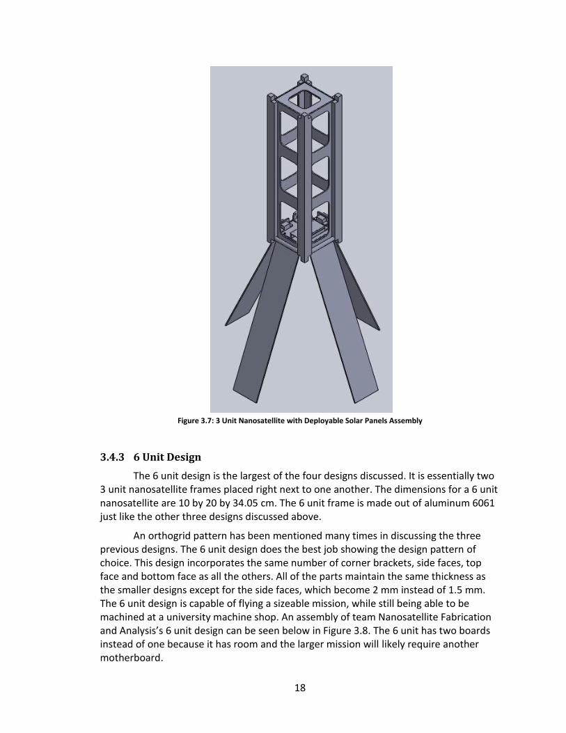
The 3 unit nanosatellite with deployable solar panel capabilities is much like the original 3 unit design but with a few modifications required for the deployable solar panels. It incorporates a bar installed into the corner brackets so that the solar panels can rotate around when they are deploying. Designing larger corner brackets takes away from a few positive parts of the team’s design. First, the corner brackets have to be thicker so that the bar can be installed into their sides. This makes the structure heavier and takes away from internal volume for the customer. With thicker corner brackets, they must become wider in order to accommodate the fasteners used to fasten the side faces to the corner brackets. This takes away from the size of the cutouts in the side faces, top face and bottom face which adds even more weight and closes down the area for the customer’s sensors or camera to see out of. The design for the 3 unit nanosatellite with deployable solar panels can be seen Figure 3.7.
On the positive side, the design does allow for solar panels to stow and deploy while staying within the P-POD requirements. It uses a simple design that can be machined at a university. The bar the solar panels rotate around is simply an aluminum dowel. The plate the deployable solar panels mount to have two small flanges with threw holes in them. The bar is put through the holes in the plate holding the deployable solar panels and installed into the holes in the sides of the corner brackets.
The outside dimensions for this design are the same as the regular 3 unit. It is also made out of aluminum 6061.
18
Figure 3.7: 3 Unit Nanosatellite with Deployable Solar Panels Assembly
3.4.3 6 Unit Design
The 6 unit design is the largest of the four designs discussed. It is essentially two 3 unit nanosatellite frames placed right next to one another. The dimensions for a 6 unit nanosatellite are 10 by 20 by 34.05 cm. The 6 unit frame is made out of aluminum 6061 just like the other three designs discussed above.
An orthogrid pattern has been mentioned many times in discussing the three previous designs. The 6 unit design does the best job showing the design pattern of choice. This design incorporates the same number of corner brackets, side faces, top face and bottom face as all the others. All of the parts maintain the same thickness as the smaller designs except for the side faces, which become 2 mm instead of 1.5 mm. The 6 unit design is capable of flying a sizeable mission, while still being able to be machined at a university machine shop. An assembly of team Nanosatellite Fabrication and Analysis’s 6 unit design can be seen below in Figure 3.8. The 6 unit has two boards instead of one because it has room and the larger mission will likely require another motherboard.

19
Figure 3.8: 6 Unit Nanosatellite Assembly
3.5 Analysis
3.5.1 Thermal
SatTherm allows students to easily input satellite and orbit properties in order to predict temperatures while in orbit. These results can then be used in the design of thermal control systems. Results from simulations of hot and cold cases for a magnetic attitude controlled nanosatellite, show that the maximum temperatures reached by the hot and cold case are 318 K and 310 K respectively. The minimum temperature reached by both cases is 260 K. Both cases reach temperatures that are outside the survival temperature ranges for certain electronics and satellite subsystems. The simulations indicate that for the specific set of satellite and orbit properties, a thermal design system needs to be implemented to keep components in their designated temperature ranges. Detailed results are located in section 6.10.
3.5.2 Modal
The modal analysis of the empty structure and assembly show that their natural frequencies are well above the required 100 Hz. The natural frequency of the empty structure is 499.4 Hz, which is 4.99 times greater than the required. The natural frequency of the assembly is 1117.5 Hz, which is 11.17 times higher than the required. These results are consistent with benchmarking cases of similar nanosatellites. Detailed results of the modal analysis simulations are located in section 7.2.

20
3.5.3 Stress at Fastener Interfaces
The expected mode of failure for the structure is the bolts shearing through the thin side faces of the nanosatellite. In order to verify that the side face design has a sufficient amount of fasteners to carry the applied loads and accelerations they are subjected to, a finite element analysis must be conducted.
Using the finite element program Marc Mentat from MSC software an analysis is done to calculate the stress on the side faces at the location of the bolt holes. In the analyses one side face is subjected to gravitational forces to simulate the acceleration of a launch. Since, this analysis isn’t of the full assembly, it is considered suitable so long as the acceleration force is significantly greater than what is expected during a launch. Hence, the analysis subjects the side face to an acceleration of 20 g. The 20 g acceleration is 3.6 times greater than the acceleration it experiences during launch. The results from the analysis show that highest stress level is 115 MPa which corresponds to a factor of safety of 2.37. Details of the set up and results of the analysis are located in section 7.3. Figure 3.9 shows the stress profile around the hole where the maximum stress occurs.
Figure 3.9: Stress Profile Around Hole Where Maximum Stress Occurs
3.6 Conclusion
The goal is to develop a range of functional nanosatellite structures capable of being machined on a university milling machine. Team Nanosatellite Fabrication and Analysis created four nanosatellite structure designs that all meet RSL, P-POD and CubeSat requirements. The four nanosatellite structural designs are 1 unit, 3 unit 3 unit deployable and 6 unit. This goal was achieved through designing a structure in SolidWorks that can be fabricated on a university milling machine. Thermal and modal analysis was also run on the design to ensure the structure would survive shipping, handling, launch, and orbit conditions. The result of this work is a functional 3 U nanosatellite with reusable fixtures to make duplicates and an easy to use thermal analysis tool.

21
Figure 3.10: Assembled Nanosatellite

22
Figure 3.11: View of the Circuit Board in the Nanosatellite

23
CHAPTER 4 – FIXTURES FOR 3 UNIT FABRICATION
Put simply, a fixture is a frame that provides support and protection for the thin nanosatellite parts while machining. Since all the parts are 2 mm thick or less, it is impossible to put them into a vice and machine them without tearing the part up with the milling tool or warping the part from the pressure of the vice. The fixtures eliminate both of those problems. The fixtures are also designed to reduce vibrations during machining. Also, for future nanosatellite fabrications the fixtures for all of the parts can be reused. All of the drawings for each fixture part can be found in Appendix VII.
4.1 Top and Bottom Face Fixture
The fixture below in Figure 4.1 is designed to machine both the top and bottom faces. This fixture consists of two parts. The first part is the bottom part of the fixture, which has outside dimensions of 120.65 by 120.65 by 25.4 mm. The bottom part of the fixture has a 12.7 mm solid base with four 12.7 mm cubes protruding from the 12.7 mm base. These cubes are designed to the height and width of the flanges on the top and bottom faces of the 3 unit nanosatellite. The base fixture also has three holes drilled and tapped in the center so that the top plate of the fixture can bolt to the base.
The top of the fixture is a 9.525 mm plate that is a 12.7 mm wider in the x and y -direction than the cutouts in the top and bottom faces. This is done to fit inside the faces and clamp down on 6.35 mm of material all the way around the cutouts. When the faces enter the fixture they are down to size in the x and y - direction so that they fit nice and snug inside the cubes coming out of the base. However, the centers of the faces are only pocketed resulting in a face cutout along with a larger pocket that accommodates the top plate with a snug fit as well. Again, the top plate grabs onto a 6.35 mm of material all the way around the cutouts.
Doing one face at a time, the face is placed inside the base plate and the top plate is placed inside the pocket made in the face. The top plate is fastened to the bottom plate using 6.35 mm coarse thread bolts. This holds the face in place and allows for the rest of the material to be removed. With everything in place, all of the excess material is removed and the faces come out with only a 2 mm thick floor and 2 mm thick flanges.

24
Figure 4.1: 1 Unit Top/Bottom Face Fixture with Completed Part
4.2 3 Unit Side Face Fixture
A two-part fixture is required to accurately and safely fabricate a 1.5 mm side face on a milling machine. The fixture designed to complete the task machines all four faces at once. A little work has to be done to bring the 4 side faces down to size in order to fit into the fixture, and holes have to be drilled in the faces in order to accommodate the six drill holes located down the center of the fixture. It can be seen below in Figure 4.2 that the six holes in the center of the fixture are in sets of two and they go all the way through to the bottom part of the fixture that is drilled and tapped. The holes are in sets of two because they go right through the three holes that are cut out of the side faces.
With the faces down to size and the holes drilled, it is time to place the parts into the fixture. The bottom part of the fixture has a trough cut out of it that creates a snug fit, once again with the part going into the fixture. The trough is 5.588 mm deep and the four faces stacked up are 6.35 mm. The trough is shallower than the faces so when the top plate is bolted down to the bottom plate by the six holes around the outside of the fixture, they clamp down on the side faces. This will keep them to move and will drastically reduce vibrations.
With everything in the fixture ready to go, three internal perimeter cuts are made; one cut is made around each of the three sets of screws. The pockets are cut right through the top plate and down through all four side faces without going beyond 10 thousands into the base plate. Once this is done, the fixture is disassembled and all four side faces come out ready for assembly. Figures 4.2 and 4.3 below show the fixture and the fixture with four side faces complete.

25
Figure 4.2: 3 Unit Side Face Fixture
Figure 4.3: 3 Unit Side Face Fixture with Completed Parts
4.3 Corner Bracket Fixture
The corner brackets were the most difficult to fabricate due to their intricate design and slenderness. The corner bracket fixture is one piece, unlike the other two fixtures, and it is designed to fabricate two corner brackets at once. Figure 4.4 shows the fixture itself. The fixture has a long pocket machined in it that holds two corner

26
brackets that start out as one piece. The corner brackets go into the fixture with the radii cut into the outside edges of the corner brackets, beveled through holes for fasteners and the cubes cut out. With the part ready for the fixture it is placed into the pocket and the cubes are clamped down at the ends as seen below in Figure 4.6.
With the aluminum bar fastened in the fixture, a pocket is then taken out of the part leaving 2 mm of material all around. At this point everything is ready except for the fact that the two corner brackets are still attached in the middle. To split the one part into two corner brackets, the clamps must be removed and the brackets must be fastened to the fixture. The brackets are fastened to the fixture using the eight drill and tap holes in the base of the trough. This will hold the parts in place while the brackets are finished. The holes in the bottom of the fixture are important because it is very dangerous to split one piece into two pieces on a milling machine. Figure 4.5 below shows the two corner brackets completed with the clamps removed.
Figure 4.4: Corner Bracket Fixture
Figure 4.5: Corner Bracket Fixture with Completed Part

27
Figure 4.6: Corner Bracket Fixture with Completed Part and Clamps

28
CHAPTER 5 – TOOL AND FASTENERS FOR 3 UNIT ASSEMBLY
5.1 Assembly Tool
Since the tolerance is so high on the 3 unit structure, an assembly tool was made to help ensure the outside most dimensions are acceptable. The tool seen in Figure 5.1 below is machined so that the outside corners of the four little pockets are exactly 10 cm by 10 cm in order to fulfill the P-POD requirements. This was made to hold the corner brackets in place while the structure is assembled with hopes of perfect outside dimensions when the tools are removed. One tool is placed on either end of the four corner brackets and engaging with the cubes to hold as best a shape as possible. The second image in Figure 5.2 shows a close up view of one of the pockets. There are two nylon tipped socket screws in the pocket so when the cubes of the corner brackets, which are smaller than the pockets, are put in, they can be pushed against the outside walls.
Figure 5.1: Assembly Tool
Figure 5.2: Assembly Tool Close Up
It can be seen in Figure 5.3 how the cubes of the four corner brackets are installed into one of the assembly tools. Figure 5.4 shows the other assembly tool exploded off the cubes for visual purposes. However, the other tool is brought down and the cubes are installed into the pockets and pressed against the back corners. This

29
should hold the corner brackets, which are in direct contact with the P-POD, at the correct location for a nice fit in the release mechanism.
Figure 5.3: Corner Brackets with One Assembly Tool
Figure 5.4: Corner Brackets with Both Assembly Tool

30
5.2 Fasteners
Due to how thin all the parts in the structural assembly are, an undercut screw must be used on one side and a captive nut must be used on the other. The machine screw is always on the outside of the frame and the captive nut is always on the inside. This is done because the screw can be made flush with a face while the captive nut cannot. The machine screw used was a 4-40 3/16 inch military specification stainless steel fastener that has an undercut on the beveled part of the screw. This is so the angle on the screw head ends and the threads start before the screw exits the face it is installed on. This will allow for the side faces to make direct contact with the corner brackets, thus creating good friction between the surfaces. Good contact between surfaces is important because the friction greatly decreases the stresses felt on the screws because the friction does not allow the face/bracket interface to move. If the interface slips it would apply a shear force on the through holes.
Figure 5.5 shows a 4-40 3/16 inch machine screw going into the outward facing part so that the screw head can sink into the face until it is just below the surface. The screw is on the left and the captive nut is on the right. The captive nut is set into the mounting hole machined into the side faces for the case seen in Figure 5.5. The captive nut is threaded with 4-40 threads and locks into the face when mounted. This allows the screw to thread into the captive nut thus securing the side face to the corner bracket. The fastener example seen below is used for the entire assembly of the structure.
Figure 5.5: Face Assembly with Fasteners
The motherboard is fastened to the structure differently. The motherboard is attached to the bottom face of the nanosatellite designs using eight 6-32 screws and four appropriate female/female standoffs. The bottom face is designed to take 6-32 undercut machine screws that are ¼ inch in length. These will be installed through the bottom face and into the 7/16 inch standoff. The motherboard is then fastened to the

31
other female side of the standoffs using 6-32 ¼ inch pan head machine screws. Figure 5.6 shows how the motherboard is fastened to the bottom face. The reason the standoffs are so high is because this allows for the circuit board ports to be accessed while the board is still attached to the bottom face. The space underneath the motherboard can be used for other parts such as additional circuit boards or batteries.
Figure 5.6: Circuit Board Assembly with Fasteners
32
CHAPTER 6 – THERMAL SYSTEM AND MAGNETIC ATTITUDE CONTROL
The electrical and mechanical components of satellite subsystems all have survival temperatures and functional temperature ranges. Therefore, it is necessary to calculate the transient temperatures of these components throughout a satellite's orbit in order to design heating or cooling systems for the components.
The following chapter explains the fundamental heat transfer and numerical methods used in the calculation of transient temperatures by the MatLab based program “SatTherm” which will be utilized and built upon to accomplish the goals set out.
6.1 SatTherm
There are several software programs that can model the orbit of a satellite and calculate the transient temperatures of nodes representing points and subsystems of a satellite. The industry standard software program is Thermal Desktop produced by C & R Technologies. Thermal Desktop is a powerful thermal analysis and modeling tool but it is expensive and can be complicated and time consuming for students to learn and become comfortable with.
A simplified software package capable of running transient thermal simulations for nanosatellites in orbit was developed by Cassandra Belle VanOutryve of San Jose State University in 2008 in conjunction with engineers at NASA Ames. The program entitled "SatTherm" consists of a group of MatLab scripts which allow the user to input physical information of the satellite, and its orbit path. The program utilizes a finite difference algorithm to approximate satellite temperatures while in orbit.
SatTherm is easy to use and it allows students to edit and add code to adapt the program for their specific project. The results from several cases attained by both SatTherm and Thermal Desktop have been compared by its developer and it is concluded that SatTherm can replicate results from Thermal Desktop to an accuracy within 4°C, which is acceptable for the early design stages of a satellite. SatTherm’s algorithms are based off of fundamental heat transfer laws and numerical methods that are discussed in the following section
One of the project's goals is to build upon SatTherm's core code to allow it to model the transient temperatures of magnetic attitude controlled nanosatellites, which is discussed in the coming sections.
6.2 Satellite Thermal Environment
In space, the sources of external heat flux onto a spacecraft are the direct radiation from the sun, infrared radiation emitted by the earth, and albedo, which is the radiation from the sun reflecting off the earth. The heat absorbed by the spacecraft is determined by the material and surface properties of the spacecraft, and its orbital path. Internal heat is generated by the electrical components of the satellite. These

33
components transfer heat to the rest of the satellite by way of conduction and radiation. The absence of a medium prevents any convection heat transfer.
6.3 Modes of Heat Transfer
6.3.1 Conduction
Conduction is the transfer of energy caused by the interactions of molecules of higher and lower energies Higher energies are associated with higher temperatures, thus in a solid object energy is transferred in the presence of a temperature gradient (Incropera, 2011). The time rate of heat conduction is characterized by Fourier's law, displayed in Eq. 6.1
(Eq. 6.1)
The variable is the heat flux in [ ], k is the transport property of the material termed thermal conductivity [ ], is the change in temperature over distance. The minus sign denotes that heat is transferred in the direction of decreasing temperature.
When analyzing the heat flux between two points, i and j, in a solid Fourier's law can be rewritten as
(Eq. 6.2)
(Eq. 6.3)
where is the total heat transfer between points i and j in watts, A is the cross-
sectional area through which the heat is flowing, L is the distance between the two
points and and are the temperatures at their respective points. The term
is the
inverse of the conduction resistance, .
6.3.2 Radiation
Thermal radiation is the emission of energy at the surface of a material as a result of its finite temperature. Unlike conduction or convection, radiation does not require the presence of a medium. It can be viewed as the transfer of energy through the propagation of photons or it can be viewed alternatively as the transfer of energy through the propagation of electromagnetic waves. For the purposes of thermal analysis in these contexts radiation is viewed as the latter case.
The amount of radiation emitted by a surface is dependent upon several factors, such as the direction and wavelength of the electromagnetic waves as well as the surface temperature. Analysis of radiation is greatly simplified by considering an idealized surface which is the perfect absorber and emitter of radiation, this idealized surface is referred to as a "blackbody". The Stefan-Boltzmann law allows for the calculation of a blackbody's emissive power as a function of temperature
(Eq. 6.4)

34
where is the Stefan-Boltzmann constant (5.67E-8 ). The results of the Stefan-Boltzmann law enables calculation of the amount of radiation emitted in all directions and over all wave lengths of a blackbody given only temperature.
As stated earlier a blackbody is an idealized surface; however, a blackbody can be used as a reference in describing emission from a real surface. Equation 6.5 gives the equation for energy emitted by a real surface, where is surface emissivity which is defined as the ratio of radiation emitted by a real surface and by a black body at the same temperature. A blackbody would have an emissivity equal to one and the more reflective a material is the lower its emissivity. Although emissivity is a function of temperature, direction, and wavelength it can be approximated as being independent of direction and wavelength.
(Eq. 6.5)
6.4 Finite Difference Temperature Solution
SatTherm utilizes a numerical method called finite difference to calculate the transient temperatures of the nanosatellite.
6.4.1 Heat Equation
The effects of heat fluxes on an objects temperature can be understood by first considering the one dimensional system under transient conditions.
(Eq. 6.6)
Where k is the materials thermal conductivity, is density and is the materials
specific heat. Equation 6.5 is referred to as the one dimensional heat equation. It is a second-order partial differential equation which relates the partial derivative of temperature with respect to time to the second partial derivative of temperature with respect to distance. In order to attain a function of temperature with respect to time and position, , numerical methods of approximation must be utilized.
6.4.2 Finite Difference Method
The finite difference method, described in Chapman, 1987, uses a forward difference approach to calculate the transient temperature of an object divided into nodes. The partial derivatives in equation 6.5 can be approximated by Taylor series expansions where higher order terms are disregarded.
(Eq. 6.7)
(Eq. 6.8)
By dividing an object into several nodes separated by and selecting one node as node n and its neighboring nodes as n-1 and n+1, becomes , becomes and becomes . Also is simply and is (The temperature of node n after one time step, ). Taking these substitutions for equations 3.6 and 3.7 and inputting them into equation 3.8 the heat equation becomes

35
(Eq. 6.9)
The next step is to multiply each side of equation 6.8 by the volume of node n,
where , substitute
with R the conduction resistance with the materials
thermal capacity, C.
(Eq. 6.10)
Equation 6.9 can be generalized to account for all nodes in direct contact with node n, allowing for analysis of systems in two dimensions.
(Eq. 6.11)
Solving for and incorporating all heat sources the explicit solution becomes
(Eq. 6.12)
Equation 6.11 shows that the transient temperature of a node can be calculated iteratively given initial temperatures and the heat fluxes at the given time. It should be noted that the value of must be bounded using associated stability criterion to insure that numerically induced oscillations are not introduced and propagated which can result in the solution going to infinity.
6.5 SatTherm Validation
The Developers of SatTherm verified the accuracy of the code by comparing several simulation cases done in SatTherm and the commercially available program Thermal Desktop. The cases consist of single and multiple node models which test the accuracy of SatTherm's heat flux calculation, contact conductance, and radiation network algorithms. Results from both programs match closely to one another, with temperature differences of approximately 4 °C (VanOutyve, 2008).
While the validation cases prove the robustness of SatTherm’s algorithms when results are compared to those of Thermal Desktop, SCU's team Nanosatellite Fabrication and Analysis conducted one additional validation case. The case is of a simple thermal balance calculation of a spherical object modeled by a single node.
The benchmarking case is of a spherical object in an orbit such that it is never in eclipse. The fact that it is never in eclipse means that all the heat fluxes remain constant and the object will reach a steady state temperature. The analytical solutions for this benchmarking case come from a lecture on spacecraft thermal design given by Dr. Christopher Kitts of Santa Clara University (Kitts, 2011). The values of all the variables involved in the case are listed in Table 6.1.

36
Variables Involved in Benchmarking Case
Variables Symbol Value
Sun Radiation Intensity
Radiation Intensity at Earth Surface
Energy Dissipated
Height Above Earth 240 km
Radius of Earth 6371 km
Visibility Factor .15
Albedo Factor .33
Area of Incident Radiation
Surface Area of a Sphere
Table 6.1: Thermal Balance Benchmarking Case Variables
The equation for the steady state temperature can be derived from the law of conservation of energy, shown in Eq. 6.13. Plugging in the equations for all the different energy sources leads to Eq. 6.16.
(Eq. 6.13)
(Eq. 6.14)
(Eq. 6.15)
(Eq. 6.16)
By rearranging Eq. 6.16 the value of the steady state temperature can be calculated and is displayed in Eq. 6.17. Plugging in the values for the sun, albedo, and earth heat fluxes, leads to Eq. 6.20 which gives the steady state temperature as a function of the ratio of the objects solar absorptivity and emissivity.
(Eq. 6.17)
(Eq. 6.18)
(Eq. 6.19)

37
(Eq. 6.20)
Figures 6.1 through 6.3 show the results of the SatTherm transient temperature values and the analytical steady state temperature calculations for three different solar absorptivity to emissivity ratios. All three graphs show that the two calculations are within 1 °C.
Figure 6.1: SatTherm and Analytical Temperatures α/ε=.13
Figure 6.2: SatTherm and Analytical Temperatures for α/ε=1

38
Figure 6.3: SatTherm and Analytical Temperatures for α/ε=44
6.6 Earth's Magnetic Field and Magnetic Attitude Control
The earth is similar to a bar magnet or a dipole, in that it has a magnetic north and south pole, which is caused by the motion of iron in Earth's liquid outer core (Freedman, 2008). The dipole causes a magnetic field that surrounds the earth, shown in Figure 6.4.
Figure 6.4: Magnetic Field Lines Surrounding Earth. Image Courtesy of NASA

39
The idea of using the Earth's magnetic field for spacecraft stabilization and attitude control was first written about in the early 1960's. White, Shigemoto, and Bourquin determined that it is possible to obtain torque about all three axes of a spacecraft, on an intermittent basis. Using torque rods, torque coils or permanent magnets the angular velocity of the spacecraft can be altered (Makovec, 2001).
6.7 Mathematical Model of Earth's Magnetic Field.
The International Association of Geomagnetism and Aeronomy (IAGA) is an organization that brings together data from magnetic field modelers and institutes that collect magnetic field data from satellites and observatories all over the world. They use the collected data to create a series of mathematical models that can approximate the force and direction of the earth’s magnetic field at points that lie between -1 km from the earth's surface to 600 km out into space. The mathematical models are referred to as the International Geomagnetic Reference Field. Due to the movement of the Earth's magnetic poles, the models are updated about every five years and are currently in the 11th generation.
6.8 Simulating Magnetic Attitude Control
MatLab has a built in function that calculates the direction and magnitude of the Earth's magnetic field at a given point and time. The function utilizes the 11th generation of the International Geomagnetic Reference Field (IGRF). This function requires the MatLab Aerospace Toolbar.
There are also sets of readily available MatLab scripts which utilize the 11th generation of the International Geomagnetic Reference Field to approximate the direction and magnitude of the Earth's magnetic field. One such set of scripts was developed by Drew Compston of Stanford University.
These scripts developed by Compston are integrated into the SatTherm code to fix the attitude of the nanosatellite so that one side is always facing in the direction of the Earth's magnetic field. The scripts generate the magnetic field line starting at a point in space and ending at a point along the magnetic field line at a given distance away. Figure 6.5 displays a graphical output of the IGRF scripts, in which a magnetic field line surrounding Earth is shown. The field line begins at a designated point in space and ends at a designated distance along the field line.
Code was added to SatTherm in order for it to utilize the IGRF code. As SatTherm goes through each time step in its calculation, it calls the IGRF scripts to calculate the direction of Earth’s magnetic field at the current position of the nanosatellite. It is setup to calculate the position of a point on the magnetic field line a small distance from the satellite's current position. Subtracting the satellite’s current position from the calculated position of the point gives a vector in the direction of the magnetic field. SatTherm sets that vector as the direction of the satellite face at that instant.

40
Figure 6.5: Magnetic Field Line Generated From IGRF Scripts
6.9 IGRF Code Validation
Code was added to SatTherm so that it would output a figure which displays a globe with the orbit path of the satellite, a vector pointing in the direction of the sun, and vectors normal to the satellite face. When the magnetic orbit orientation is selected, the direction of the vectors normal to the nanosatellite face is the direction of the earth's magnetic field.
When the nanosatellite orbit has a zero degree inclination the magnetic field vectors are expected to point upward. When the orbit has a 90 degree inclination the nanosatellite should make two revolutions about its own axis, per orbit period. It points into the earth near the North Pole and away from the earth near the South Pole. Figures 6.6 and 6.7 show that the results of these two cases are precisely what they are expected to be.
Figure 6.6: Magnetic Attitude Control Orbit with 0ᵒ Inclination

41
Figure 6.7: Magnetic Attitude Control Orbit with 90ᵒ Inclination
6.10 Magnetic Attitude Controlled Orbit Simulations
Simulations were run to calculate the transient temperatures of a nanosatellite orbit for hot and cold cases of a magnetic attitude controlled orbit. The optical properties of the satellite were the same as the GeneSat-1 nanosatellite. The outside surface of the GeneSat-1 consisted of solar cells and gold coated aluminum. The weighted averages for the solar absorptivity and emissivity of the two surface materials were .509 and .588 respectively (VanOutryve, 2008). An internal heat load of 5 watts was placed on the bottom face of the nanosatellite (node number 2).The orbit properties are displayed in Table 6.2.
Values for Hot and Cold Cases Run
Hot Case Cold Case
Solar Heat Flux 1414 W/m² 1332 W/m²
Earth IR Heat Flux 257 W/m² 218 W/m²
Albedo Factor 0.33 0.19
Orbit Inclination 40° 40°
Altitude 500 km 500 km
Eccentricity 0 0
RAAN 60° 60°
Argument of Perigee 270° 270°
RA Sun 247° 247°
Dec Sun -21° -21°
Table 6.2: Orbit Properties for Hot and Cold Cases

42
The max temperatures reached by the hot and cold cases were 318 K and 310 K respectively. The minimum temperatures reached were both 260 K. Both cases reached temperatures that are outside the range for survival temperature for electronics and satellite subsystems. The simulation data can be used for designing thermal control systems. Figures 6.8 and 6.9 show the graphs for the transient temperatures of the hot and cold cases. The six lines on the graphs are for each of the six sides of the nanosatellite.
Figure 6.8: Orbit Cold Case
Figure 6.9: Orbit Hot Case
6.11 Thermal Analysis Future Work
SatTherm does not currently have a complete graphical user interface. It runs by defining all the necessary variables in an m-file and calling the function that calculates the transient temperature. A semi functional graphical user interface was developed but never completed, because of difficulties assigning variables which were not constant for all of the nodes in the model.

43
CHAPTER 7 – FINITE ELEMENT ANALYSIS
7.1 Modal Analysis
Modal Analysis is the process of determining the inherent dynamic characteristics of a system in forms of natural frequencies, damping factors and mode shapes (He, 2001). These dynamic characteristics are determined by the structure or part's mass, stiffness and damping.
7.2 Modal Analysis Simulation
7.2.1 Structure Modal Analysis
Modal analysis is conducted using the finite element program Ansys v13. To compare the results to other modal analysis results of nanosatellite structures the structure itself with no interior parts is examined. The natural frequency for the IRIS structure developed at Santa Clara University in 2008 and 2009 has a natural frequency of about 350 Hz. Since IRIS weighed considerably more than the 3 unit nanosatellite being analyzed, it is expected that the 3 unit nanosatellite have a higher natural frequency.
The model’s boundary conditions mimic the constraints applied to the nanosatellite while in a P-POD. The eight corners are constrained to have no displacement in any direction. Figure 7.1 displays the model with its zero displacement boundary conditions.
Figure 7.1: Zero Displacement Boundary Condition at Eight Corners
The results of the modal analysis show that the structure has a natural frequency of 499.4 Hz which as predicted is greater than that of the IRIS nanosatellite and exceeds the required frequency of 100 Hz. The program also calculates the frequency for five other modes resulting in frequencies of 531.9 Hz, 536.5 Hz, 581.5 Hz 717.2 Hz and 791.4 Hz for modes 2 through 5 respectively. Table 7.1 shows the frequency results of the analysis.

44
First 6 Modal Frequencies of Structure
Mode Frequency (Hz)
1 499.4
2 531.9
3 536.5
4 581.5
5 717.2
6 791.4
Table 7.1: Frequency Results for Modal Analyses of Structure
Since the side panels of the structure are thin, it is expected that the dominant mode of vibration be at the slender horizontal sections of those panels. The mode shapes show that in fact the structure does vibrate in this manner. Figure 7.2 shows the mode shapes for the first six modes.
Figure 7.2: Mode Shapes for Structure Modal Analysis

45
7.2.2 Assembly Modal Analysis
Along with running a modal analysis on the structure alone an analysis was run on the structure containing a micro controller and payload housing in the interior and thin aluminum plates which covered the exterior. Figure 7.3 shows the assembly of the structure.
Figure 7.3: Complete Assembly of Structure (left). Structure with Outside Plates Hidden to Show Interior Components (right)
The model was given the same zero displacement boundary condition at the eight corners as the structure in section 7.2.1. Although this assembly has more mass than the previous structure it should have a higher natural frequency because the extra components make it considerably stiffer. The results showed that the natural frequency was 1117.5 Hz. The program also calculated the frequency for five other modes resulting in frequencies of 1118.3 Hz, 1291.6 Hz, 1330.6 Hz, 1417.1 Hz and 1425.2 Hz for modes 2 through 5 respectively. Table 7.2 shows the frequency results of the modal analysis.
First 6 Modal Frequencies of Assembly
Mode Frequency (Hz)
1 1117.5
2 1118.3
3 1291.6
4 1330.6
5 1417.1
6 1425.2
Table 7.2: Frequency Results for Modal Analysis of Assembly

46
The mode shapes for the previous structure (see Figure 7.2) showed that the vibrations would dominate at the slender horizontal sections of the side brackets. In the assembly those sections are constrained by the interior payload housing. For the assembly the mode shapes would be expected to show vibrations at the outside panels that cover the structure. Figure 7.4 does in fact show that the vibrations occur on the outside panels.
Figure 7.4: Mode Shapes for Assembly Modal Analysis
7.2.3 Modal Analysis Conclusion
The modal analysis of the empty structure and assembly conducted using Ansys v13 show that their natural frequencies are well above the required 100 Hz. The natural frequency of the empty structure is 499.4 Hz, which is 4.99 times greater than the required. The natural frequency of the assembly is 1117.5 Hz, which is 11.17 times higher than the required.
7.3 Analysis of Stress at Fastener Interfaces
The expected failure mode for the nanosatellite is a bolt shearing through the thin aluminum side faces. Analysis on the shearing of the side faces is done using the finite element program Marc Mentat from MSC software.

47
The model consists of 3724 nodes. The nodes along the top half of each screw hole are bounded in all directions to simulate the constraints the holes are subjected to by screws. Figure 7.5 displays the boundary conditions at the holes.
Figure 7.5: Side Face Boundary Conditions
The analysis subjects the side face to gravitational forces to simulate the acceleration of a launch. Launch vehicles, such as an Atlas rocket, reach accelerations of up to 5.5 g. Since this analysis isn’t of the full assembly it is considered suitable if the acceleration force is significantly greater than what is expected during a launch. Hence, the analysis subjects the plate to an acceleration of 20 g, which is 3.6 times greater than the force expected during launch.
The results show that the maximum stress occurs at one of the holes in the second row of holes from the bottom. It would be expected that the highest stress would occur at the lower hole, but since there are only two holes in the second row from the bottom, those two holes each carry a greater load. The maximum stress value is 115 MPa. Figure 7.6 displays the stress profile at the maximum stress area. The yield strength of aluminum 6061-T6 is 273 MPa, which leads to a safety factor of 2.37.
Figure 7.6: Stress Profile at Maximum Stress Area

48
7.3.1 Stress Analysis Conclusion
Although the stress analysis model is overly simplified, it is subjected to acceleration 3.6 times greater than it would experience during a launch. The maximum stress at a 20 g acceleration is 115 MPa which results in a safety factor of 2.37. Although the results indicate that the design would be able to survive a launch only a physical vibration test can actually guarantee, with an acceptable level of confidence, that the nanosatellite will in fact survive a launch.

49
CHAPTER 8 – COST ANALYSIS
The overall costs to design and fabricate a nanosatellite structure can be expensive. The team’s goal is to lower the cost by machining every component here at Santa Clara University. The costs include material costs for the fixtures and parts, fasteners for assembly and fixtures, and tools for machining the structure. The cost of the team’s 3 unit nanosatellite structure is 545 dollars for everything. Pumpkin Inc.’s 3 unit nanosatellite costs nearly 9,000 dollars. The team’s costs mainly come from the material for the fixtures and the milling tools. Since the fixtures and milling tools are reusable, futures costs will be even less. Labor costs are kept down because all the machining is done by students.
50
CHAPTER 9 – BUSINESS PLAN
9.1 Introduction
The nanosatellite industry is small and mainly revolves around NASA and university programs. It is very difficult and expensive to put a nanosatellite into space and therefore it does not happen all too often. Team Nanosatellite Fabrication and Analysis has designed four different sized nanosatellite structures: 1 unit, 3 unit, 3 unit deployable and 6 unit. A unit is defined as 10 by 10 by 11.34 centimeters. Due to the small market for nanosatellite frames and a company named Pumpkin Inc. that is the leader in the frame industry; the team’s designs will be used for future university programs.
9.2 Goals and Objectives
The goal of the team is to produce a 3 unit nanosatellite structure comparable to that of the commercial nanosatellite manufacturing company, Pumpkin Inc., using only the tools available in the university’s machine lab. The structure has to have a simple design to allow for machinability using only a milling machine.
Money and commercial aspirations are not a focus of the team because the market for nanosatellite structures is too small. The purpose of the project is purely educational, allowing students to gain hands on experience in the design and manufacturing processes required to build a structure under the given design constraints and manufacturing limitations.
9.3 Product Description
The products produced by team Nanosatellite Fabrication and Analysis are great for university nanosatellite programs interested in machining their own nanosatellite structures. The team created four structural designs: 1 unit, 3 unit, 3 unit deployable and 6 unit. All four designs contain the same four design components; the four components in the designs are corner brackets, side faces, a top face and a bottom face. There are four corner brackets, four side faces, a top face and a bottom face. The corner brackets are 2 mm thick and run in the vertical direction as seen in Figure 9.1. All the faces have an orthogrid pattern, which is a rectangular cutout where the pattern is square to the frame and the design is square to itself. The side faces for a 3 unit are roughly 1.5 mm and the top and bottom faces are 2 mm. The bottom face is the only non-orthogrid face. All the other faces have an orthogrid pattern and fasten together. The bottom face is interesting because it was designed to attach the circuit board directly. Attaching a motherboard is great because the customer can simply attach their components and use the motherboard installed. The circuit board can also be seen in Figure 9.1 below. It is also important to know that all of the designs can be fabricated on a university milling machine.

51
Figure 9.1: 3 Unit Nanosatellite Assembly
9.4 Potential Market
The potential consumers for nanosatellite structures are university programs and research institutions that are interested in doing scientific experiments and research in space. This is a very small market, which already has an established supplier, Pumpkin Inc.
Pumpkin Inc.’s products are made using sophisticated manufacturing processes and tools that require significant initial investments to produce. These initial investments only payoff once the company’s sales surpass that initial investment. In such a small market with an already established supplier it would be a very risky venture and possibly unwise decision to attempt to break into the market.
The only reason the team’s structure will cost less than a Pumpkin Inc. product is because the only expenses are the raw materials, fasteners and machining tools. The tools and machinery used are from the university’s machine lab and the time and labor is put in by students.

52
9.5 Manufacturing
There are many positive things that come along with the manufacturing of a design created by the team. To start, each design is made so the entire system can be fabricated on a milling machine. When manufacturing one of the designs there is a lot of work to do and a lot of very important detail to pay attention to. Since the frame ranges from 1.5 to 2 mm in thickness for the 3 unit, fixtures need to be created in order to protect the thin components that form the structure. Fortunately, team Nanosatellite Fabrication and Analysis created fixtures for all four components all of which can be reused by Santa Clara University or created by other universities from the drawings the team produced.
The entire structure is made out of aluminum 6061 and it is machined on a milling machine. The manufacturing will be done entirely by those directly involved with the project. The idea was to give universities a model to produce a nanosatellite frame for a low cost. Another benefit with fabrication is the students will gain a positive perspective into the reality of designs for manufacturability, fabrication and assembly.
9.6 Product Cost
Production cost of university nanosatellite programs tends to be very high. They survive due to generous donations from companies such as Lockheed Martin and NASA. To purchase a 3 unit nanosatellite from Pumpkin Inc. is around 9,000 dollars; team Nanosatellite Fabrication and Analysis was able to fabricate a frame for 545 dollars. The 545 dollars included tools Santa Clara University did not have, such as fasteners for fixtures and assembly and materials for fixtures and structural components. The cost breakdown can be seen in Appendix V.
9.7 Future Financials
Since the team’s project is directed toward future university nanosatellite programs, the financials in the future relate to the costs to produce a nanosatellite frame. If a frame is to be purchased costs increase, but if the frame is fabricated in a university machine shop the team will not require nearly as much financial assistance. If a frame is purchased, the cost is around 9,000 dollars. If one is machined at a university then it will cost less than 100 dollars.
In order to continue finances, university programs must do a good job producing results each year. Companies will not continue to donate money for educational purposes if the school receiving the money is not doing anything with it. Work hard, produce results and people will enjoy and continue donating.

53
CHAPTER 10 – ENGINEERING STANDARDS AND CONSTRAINTS
Team Nanosatellite Fabrication and Analysis’s project, includes 1 to 6 unit nanosatellites. A single unit is 10 by 10 by 11.34 cm and can weigh up to 1.33 kg. The team is designing 1 to 6 unit nanosatellites along with fabricating and analyzing a 3 unit nanosatellite, with the goal of at least one design making it to space. When a satellite is launched into space there are some major areas of impact, some positive and some negative. The first area of impact is space itself. Space junk, old broken space systems, is one of the largest concerns in space right now. Another impact area is launch because lots of rocket fuel is burned in our atmosphere and rockets have failed to make it to space resulting in a crash landings on earth. An additional area of impact is the large range of research nanosatellites can provide such as earthquake detection methods for those on earth. Impacts such as the manufacturability, safety and economics were also looked at.
10.1 Social
Nanosatellites can be used for different types of research. Back in 2006 NASA realized the potential of nanosatellites for deep space observation, biological research, earthquake measurements and even earth observation. These research missions can have many social impacts. The earthquake measurement missions can better predict earthquakes from space to help with warning and preparation.
10.2 Manufacturability
A major focus and concern of the project is machinability. Designs had to take into account the limitations of using only a milling machine. As parts are machined, more is learned about machining limitations. In order to eliminate those limitations, tools are created to make machining individual parts easier. Another important factor in the machining of the parts is safety. Many safety precautions are taken to ensure the safety of the people machining the parts.
10.3 Economics
The fact that everything is machined in-house improves the economic impact by reducing the cost. The cost of the project resides in the stock aluminum and fasteners. Since students are machining the project, the cost of labor is removed.
10.4 Environmental
According to NASA Orbital Debris Program Office, 95 percent of everything launched into space is no longer functional. When there is a lot of space debris it becomes more dangerous for functional satellites because they run a higher risk of getting hit by space debris. There have been thousands of space launches over the decades. Some debris has burned up in Earth’s atmosphere and thousands of others are still out there. Unfortunately, sometimes they do not burn up completely and they can fall through our atmosphere and land on earth possibly injuring those in society, however, for nanosatellites this is not a problem. Space Surveillance Network is a US
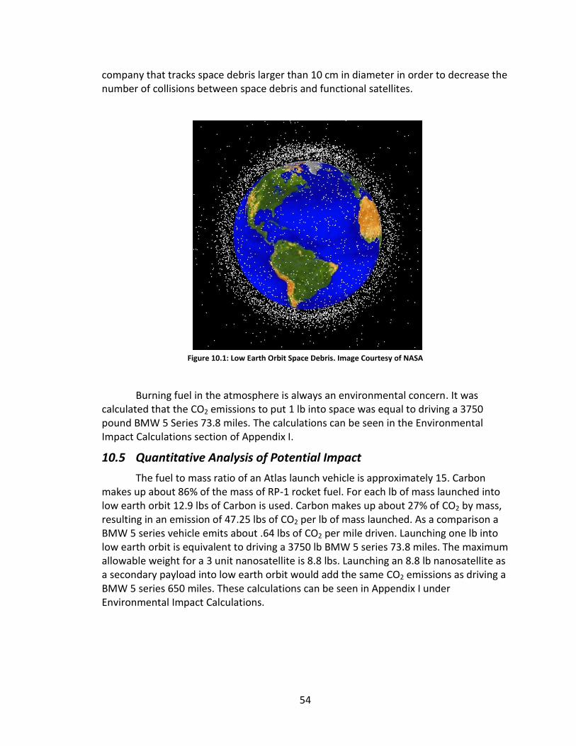
54
company that tracks space debris larger than 10 cm in diameter in order to decrease the number of collisions between space debris and functional satellites.
Figure 10.1: Low Earth Orbit Space Debris. Image Courtesy of NASA
Burning fuel in the atmosphere is always an environmental concern. It was calculated that the CO2 emissions to put 1 lb into space was equal to driving a 3750 pound BMW 5 Series 73.8 miles. The calculations can be seen in the Environmental Impact Calculations section of Appendix I.
10.5 Quantitative Analysis of Potential Impact
The fuel to mass ratio of an Atlas launch vehicle is approximately 15. Carbon makes up about 86% of the mass of RP-1 rocket fuel. For each lb of mass launched into low earth orbit 12.9 lbs of Carbon is used. Carbon makes up about 27% of CO2 by mass, resulting in an emission of 47.25 lbs of CO2 per lb of mass launched. As a comparison a BMW 5 series vehicle emits about .64 lbs of CO2 per mile driven. Launching one lb into low earth orbit is equivalent to driving a 3750 lb BMW 5 series 73.8 miles. The maximum allowable weight for a 3 unit nanosatellite is 8.8 lbs. Launching an 8.8 lb nanosatellite as a secondary payload into low earth orbit would add the same CO2 emissions as driving a BMW 5 series 650 miles. These calculations can be seen in Appendix I under Environmental Impact Calculations.

55
CHAPTER 11 – CONCLUSION
The team objective was to provide Santa Clara University the ability to rapidly design, fabricate and analyze 1-6 unit nanosatellite structures. The design, fabrication and analysis process is made so the structure can be completed at Santa Clara University. The team encountered many problems when trying to create a structure capable of being machined in a university machine shop that also met RSL, P-Pod, and CubeSat requirements.
The team developed a system that allows for four different nanosatellite structures to be fabricated on a university milling machine. The designs for the fixtures to build the parts for the nanosatellite structure and the parts for the structure itself were all successfully designed using SolidWorks. Fabrication of the 3 unit nanosatellite turned out to be a complete success. The structure meets all of the RSL, P-POD and CubeSat requirements. The designs can be machined at SCU and all the fixtures are reusable. RSL now has the ability to design to mission specifications and fabricate the structure here at Santa Clara for less than 100 dollars, while Pumpkin Inc. will cost a university roughly 9,000 dollars.
Using finite element software to conduct modal analysis the team attained results similar to other benchmarking cases. The natural frequency of the structure was found to be 499 Hz, which is well above the 100 Hz level. Finite element analysis was also done on the structure to ensure that the plate thickness used and the amount of bolts used to fasten parts together would allow the structure to survive a launch. The analyses subjected a single 3 unit side face to a gravitational load of 20g which is 3.6 times greater than the acceleration it would be exposed to during a launch. The results showed that the structure would survive with a safety factor of 2.37.
The thermal analysis tool SatTherm was used to run preliminary thermal simulations of specific orbits. Code was added to the program to enable it to calculate the direction of the earth’s magnetic field and simulate a nanosatellite which uses magnetic attitude control. This analysis tool is now available to future nanosatellite teams at Santa Clara University who will also be able to add to the code and use it for the design of thermal control systems.
Nanosatellites have proven to be valuable educational tools. Engineers in the aerospace industry value university nanosatellite programs because they give students hands on experience with spacecraft development which prepare engineers as they enter the industry.
11.1 Future Work
With the nanosatellite frame completed, there are areas that need to be worked on in the future in order to reach an overall goal of a mission launch. Physical tests, customization for internal components and a SatTherm graphical user interface would all better the project.

56
Simulations are not accepted by NASA as validation, they require physical tests. Team Nanosatellite Fabrication and Analysis did simulations to analyze the frame, but to properly validate the nanosatellite, physical tests need to be conducted. Both thermal and vibration tests need to be performed to ensure the nanosatellite’s survival during launch.
Since a nanosatellite is meant for research it needs to accommodate internal components. Team Nanosatellite Fabrication and Analysis’s frame needs to be modified to mount any internal components. The frame was designed so that fastener holes can be implemented into the faces and corner brackets by simply putting the parts back into their appropriate fixtures. This was done so that the frame could be customized to the parts going inside. The main complaint about Pumpkin Inc. is that their premade mounting holes are hard to work with.
The frame can be adapted to fit just about any mission and the frame can also be re-created for less than 100 dollars. This can be done by using the reusable fixtures team Nanosatellite Fabrication and Analysis provided SCU with. The team also ran simulations that support the decisions made in the design and fabrication process; however, thermal and vibration test must be run on the system for launch approval.

57
BIBLIOGRAPHY
Aparicio, Emmanuel, Katherine Byrne, TJ Leising, Jason Takisaki, Reyn Wakabayashi, and Anthony Young. "NANOSATELLITE MECHANICAL DESIGN AND ANALYSIS." Thesis. Santa Clara University, 2009. Print.
Clements, Twyman Samuel. "INITIAL DESIGN, MANUFACTURE, AND TESTING OF A CUBELAB MODULE FRAME FOR BIOLOGICAL PAYLOADS ABOARD THE INTERNATIONAL SPACE STATION." Mater's Thesis. University of Kentucky, 2011. Web.
<http://uknowledge.uky.edu/gradschool_theses/106>.
Compston, Drew. International Geomagnetic Reference Field (Igrf) Model. Program documentation. Mathworks.com/matlabcentral. Vers. 2012. MathWorks, 25 Apr. 2012. Web. May 2012. <http://www.mathworks.com/matlabcentral/fileexchange/34388-international-geomagnetic-reference-field-igrf-model>.
CubeSat Design Specification. Rep. California Polytechnic State University, 1 Aug. 2009. Web. Oct. 2011.
<http://www.cubesat.org/images/developers/cds_rev12.pdf>.
Dunn, Bruce. "Liquid Fuels." Liquid Fuels. NASA, 1997. Web. 26 June 2012. <http://settlement.arc.nasa.gov/Nowicki/SPBI1LF.HTM>.
Finlay, Christopher. "IAGA V-MOD Geomagnetic Field Modeling: International Geomagnetic Reference Field IGRF-11." National Geophysical Data Center. National Oceanic and Atmospheric Administration, 28 Jan. 2010. Web. Apr. 2012. <http://www.ngdc.noaa.gov/IAGA/vmod/igrf.html>.
Freedman, Roger A., and William J. Kaufmann. Universe. 8th ed. New York, NY: W.H. Freeman and, 2008. Print.
Greenberg, Andy. "Nanosatellites Take Off." Forbes. Forbes Magazine, 22 Nov. 2010. Web. Nov. 2011.
<http://www.forbes.com/forbes/2010/1122/technology-pumpkin-inc-andrew-kalman-toasters-in-space.html>.
He, Jimin, and Zhi-Fang Fu. Modal Analysis. 1st ed. Oxford: Butterworth-Heinemann, 2001. Print.
Humphery, Betty. "NASA - Advanced Space Transportation Program Fact Sheet." NASA.gov. NASA. Web. 26 June 2012. <http://www.nasa.gov/centers/marshall/news/background/facts/astp.html_prt.htm>.
Incropera, Frank P., David P. DeWitt, Theodore L. Bergman, and Adrienne S. Lavine. Fundamentals of Heat and Mass Transfer. 7th ed. John Wiley & Sons, 2011. Print.

58
Jacques, Lionel. "Thermal Design of the Oufti-1 Nanosatellite." Thesis. University of Liège, 2009. Print.
"John F. Kennedy Space Center -Â KSC Fact Sheets and Information Summaries." KSC Facts. NASA, 28 Aug. 2002. Web. Apr. 2012.
<http://www-pao.ksc.nasa.gov/kscpao/nasafact/count2.htm>.
Kalman, Andrew E. "Recent Advances in the CubeSat Kit Family of Picosatellites." 19th Annual AIAA/USU Conference on Small Satellites in Logan, Utah on August 6, 2005. Web. May 2012. <http://www.cubesatkit.com/docs/press/pumpkin_smallsat_conf_20050806.pdf>.
Kitts, Christopher. "Satellite Thermal Environment." Spacecraft Thermal Design. Santa Clara University, Santa Clara. 2011. Lecture.
""Leaked" Investor Info on Atlantic." "Leaked" Investor Info on Atlantic. Fisker Buzz, 17 May 2012. Web. May 2012. <http://fiskerbuzz.com/forums/Thread-Leaked-investor-info-on-Atlantic>.
Makovec, Kristin L. "A Nonlinear Magnetic Controller for Three-Axis Stability of Nanosatellites." Thesis. Virginia Polytechnic Institute and State University, 2001. Print.
Micciché, P., G. Bitetti, S. Mileti, M. Marchetti, P. Coluzzi, and F. Mazza. "DEVELOPMENT AND VALIDATION OF A NEW FACILITY FOR LOW EARTH ORBIT THERMAL CYCLING SIMULATION." Wiley Online Library. Society for Experimental Mechanics, 9 Oct. 2009. Web. 26 June 2012.
<http://onlinelibrary.wiley.com/doi/10.1111/j.1747-1567.2008.00417.x/full>.
Nguyen, Hugo, Robert Thorslund, Greger Thornell, Johan Kohler, and Lars Stenmark. "Structural Integrity of Flat Silicon Panels for Nanosatellites: Modeling and Testing." Journal of Spacecraft and Rockets 43.6 (2006): 1319-327. Uppsala University, 16 May 2006. Web. May 2012. <http://urn.kb.se/resolve?urn=urn:nbn:se:uu:diva-94641>.
Pariente, Meidad. "Nanosatellite Industry Overview." SlideShare. SPACECIALIST, 23 Apr. 2012. Web. 21 May 2012
<http://www.slideshare.net/mpariente/nanosatellite-industry-overview>.
Passerone, Claudio, Maurizio Tranchero, Stefano Speretta, Leonardo Reyneri, Claudio Sansoè, and Dante Del Corso. "Design Solutions for a University Nano-satellite." (2008). Print.
Pisacane, Vincent L. Fundamentals of Space Systems. 2nd ed. Oxford: Oxford UP, 2005. Print.
Preumont, André. Random Vibration and Spectral Analysis. 1st ed. Dordrecht: Kluwer Academic, 1994. Print.

59
Richmond, John Anger. "Adaptive Thermal Modeling Architecture for Small Satellite Applications." Master's Thesis. Massachusetts Institute of Technology, 2010. Print.
Shirgur, Badrinarayan, and Derek Shannon. "The Design and Feasibility Study of Nanosatellite Structures for Current and Future FSI Micromissions." Thesis. University of Central Florida. Print.
Stevens, Craig L. "Design, Analysis, Fabrication, and Testing of a Nanosatellite Structure." Master's Thesis. Virginia Polytechnic Institute and State University, 2002. Print.
Toorian, Armen, Ken Diaz, and Simon Lee. The CubeSat Approach to Space Access. Rep. Web. Nov. 2011.
USA. Air Force Research Laboratory. Nanosat-5 User’s Guide. University of Minnesota, Feb. 2007. Web. Oct. 2012. <https://wiki.umn.edu/pub/AeroDesign2Nanosat/BackgroundDocs/UN5-0001_NS5UsersGuide_Rev-.pdf>.
VanOutryve, Cassandra Belle. "A Thermal Analysis and Design Tool for Small Spacecraft." Master's Thesis. San Jose State University, 2008. Print.

60
APPENDIX I – DETAILED CALCULATIONS
Environmental Impact Calculations

61
SatTherm Code
The following MatLab code is the SatTherm program which was developed by Cassandra Belle VanOutryve and engineers at NASA AMES. VanOutryve’s thesis, "A Thermal Analysis and Design Tool for Small Spacecraft" Outlines the numerical methods and heat transfer principles and orbit parameters involved in calculating transient temperatures during an orbit. It also contains a user’s manual which explains each variable that goes into the calculations.
The Figure below displays the local coordinates and node names as they are referred to in the SatTherm code. (Outside faces should be solid)
Figure I.1: Satellite Local Coordinates & Node Names
Input Script (Not Included in Original Satherm Code)
%%%%%%%%%%Inputs to trans_temp.m
% This script is used to input all the satellite and orbit Data needed to run SatTherm
clear all
close all
clc
%----------------------------------------------------------Simulation Time
delta_t=.5; %time step <s>
min=300; % Duration <min>
t_final=60*min; %Duration <s>

62
year=2012;
month=06;
day=16;
%-------------------------------------------------------------Orientations
orientation='Magnetic';
rotation_axis='+Z'; %axis of rotation
shape='Rectangle'; %satellite shape
nodename=['S1'; 'S2'; 'S3'; 'S4'; 'S5'; 'S6']; %Node Names
ntot=6; %total side, 6 for rectangular
%---------------------------------------------------------Orbit Properties
inc=40; %Orbit Inclination <deg>
raan=60; %Right Ascension of Ascending Node <deg>
arg_peri=270 %Argument of Periapsis <degree>
max_alt=500; %Altitude above Earth <km>
ecc=.0; %eccentricity of elliptical orbit
setraddec=15; % Right Ascension and Declination, for orientaion option
% Set R.A. and Dec
%--------------------------------------------------Earth and Sun Properties
Re=6378.137; %Radius of Earth <km>
mu=398601; %Earth Gravitational Parameter <km^3/s^2>
Te=249; %Earth Temperature
AF=.19; %Albedo Factor
Gs=1332; %Solar Constant <W/m^2>
RAsun=25; %Right Ascension of Sun
Decsun=20; %Declinatrion of Sun
%-----------------------------------------------------Satellite Properties
A=[.01 .01 .03 .03 .03 .03]; %Surface Area of each side <m^2>
th=[.002 .002 .002 .002 .002 .002]; %thickness <m>
rho=[2700 2700 2700 2700 2700 2700]; %density <kg/m^3)
cp=[896 896 896 896 896 896]; %Specific Heat <J/(kg*K)>
abso_sol=[.44 .44 .44 .44 .44 .44]; %Solar Absorbtivity
emis_ir=[.01 .01 .01 .01 .01 .01]; %IR emissivity
temp_init=[295 295 295 295 295 295]; %Initial Temp (K)

63
temp_init(:,:)=298;
inthl=[0 5 0 0 0 0]; %Internal Heat Load <W>
%Conductance Matrix, Contact Conductance, <W/K>
%Note: Usually given as h_c,in W/m^2-K,
%for Aluminum with milled and clean surfaces
%h_c=1730 W/m^2 K
%Contact Areas
CA=[ 0 0 0.2000 0.2000 0.2000 0.2000;
0 0 0.2000 0.2000 0.2000 0.2000;
0.2000 0.2000 0 0.6000 0 0.6000;
0.2000 0.2000 0.6000 0 0.6000 0;
0.2000 0.2000 0 0.6000 0 0.6000;
0.2000 0.2000 0.6000 0 0.6000 0].*1e-3;
conductance=CA.*1730;
% % % Radiation View Factors Matrix for 3U
% % % See ViewFactor_Calc.m
rad_vf=[0 0.0330 0.0806 0.0806 0.0806 0.0806;
0.0330 0 0.0806 0.0806 0.0806 0.0806;
0.0806 0.0806 0 0.2570 0.3247 0.2570;
0.0806 0.0806 0.2570 0 0.2570 0.3247;
0.0806 0.0806 0.3247 0.2570 0 0.2570;
0.0806 0.0806 0.2570 0.3247 0.2570 0];
%-----------------------------------------------------------------Rotation
spins=0; %Spin per minute
a=(Re+max_alt)./(1+ecc); %orbit semi-major axis
P=2.*pi .*sqrt(a^3/mu); %orbit period
rotation= (360*spins)*P/60;
%-----------------------------------------------------------------Function
Trans_Temp=trans_temp(t_final,delta_t,shape,inc,raan,arg_peri,max_alt,ecc,orientation,setraddec,rotation,rotation_axis,Re,mu,Te,AF,Gs,RAsun,Decsun,ntot,A,th,rho,cp,abso_sol,emis_ir,temp_init,inthl,conductance,rad_vf,nodename,year,month,day);

64
Main Script, Solver
% Calculate Transient Temperatures
function [t,temp]=trans_temp(t_final,delta_t,shape,inc,raan,arg_peri,max_alt,ecc,orientation,setraddec,rotation,rotation_axis,Re,mu,Te,AF,Gs,RAsun,Decsun,ntot,A,th,rho,cp,abso_sol,emis_ir,temp_init,inthl,conductance,rad_vf,nodename,year,month,day)
tic
close all
V=A.*th; %node volumes
C=rho.*V.*cp; %node thermal capacities
sigma = 5.6704e-8; %Steffan Boltzmann const (W/(m~2 K)
r_sun=RADec2geocen(RAsun,Decsun,149598000); %geocen pos of sun (km)
a=(Re+max_alt)./(1+ecc); %orbit semi-major axis
P=2.*pi .*sqrt(a^3/mu); %orbit period
if P/delta_t <= 2.*rotation/360;
disp('Warning: Aliasing may occur. The sampling rate is less than the Nyquist Rate for the spacecraft rotation. The time step-sizeshould be decreased, or the rotation should be decreased.')
end
%Radiation Network
Res_self_inv = (A.*emis_ir)./(1-emis_ir);
%l/Ri=((l-eps_i)/(A_i*eps_i))~-l Cengel Eqn. 9-44
Res_other_inv = (repmat(transpose(A),1,ntot).*rad_vf);
%l/Rij = (l/Ai*Fij)~-l Cengel Eqn. 9-49
Res_mat = Res_other_inv; %Begin building Resistance Network matrix
for j=1:ntot %continue building Resistance Network Matrix
Res_mat(j,j)=-Res_self_inv(j)-sum(Res_other_inv(j,:));
end
%Figure out how many sides there are (outside panels)
switch shape
case 'Rectangle'
nsides=6;
case 'Hexagon'
nsides = 8;

65
case 'Octogon'
nsides = 10;
otherwise
disp('Error: Invalide Shape Option.')
end
temp_old=reshape(temp_init,1,1,ntot); %set initial temp*****************
t_old=0;
delta_t_old=delta_t;
k_old=0;
N = t_final./delta_t; %number of timesteps
%initialize arrays, to be filled in the loop
l=1;
t = zeros(floor(N+1),1,1);
r_sc = zeros(floor(N+1),3,1);
v_sc = zeros(floor(N+1),3,1);
XYZ_geoc1=zeros(floor(N+1),3);
S = zeros(floor(N+1),3,1);
PF= zeros(floor(N+1),3,1);
zloc = zeros(floor(N+1),3,1);
xloc = zeros(floor(N+1),3,1);
yloc = zeros(floor(N+1),3,1);
n = zeros(floor(N+1),3,ntot);
n_inloc = zeros(floor(N+1),3,ntot);
n_inloc_rot = zeros(floor(N+l),3,ntot);
qext_arr = zeros(floor(N+l),3,ntot);
Qext = zeros(floor(N+l),l,ntot);
Qspace = zeros(floor(N+l),l,ntot);
Qcond = zeros(floor(N+l),l,ntot);
Qrad = zeros(floor(N+l),l,ntot);
Qint = zeros(floor(N+l),l,ntot);
latT = zeros(floor(N+1),3,1);
temp = zeros(floor(N+l),l,ntot);
delta_t_lim = zeros(floor(N+l),l,ntot);

66
delta_t_lim_min = zeros(floor(N+l),1,1);
tcheck_sum = zeros(floor(N+l),1,1);
delta_t_new = zeros(floor(N+1),1,ntot);
%------------------------------------
while t_old < t_final
k=k_old+l;
percent=t_old/t_final*100
t(k,:) = t_old+delta_t_old;%current time (s)
[r_sc(k,:),v_sc(k,:)] = geocen_rv(inc,raan,arg_peri,max_alt,ecc,t(k,:)); %***********************
%current position & velocity vects (km) and (km/s)
perp_2_orbit_plane = cross(r_sc(k,:),v_sc(k,:));
%a vector that is perpendicular to the plane of the orbit
S(k,:) = r_sun-r_sc(k,:);
%line of sight vector between spacecraft and sun (km)
%Define the Spacecraft local axes, xloc,yloc,zloc, in geocen-eq.
%corrdinates. zloc is either sun-facing, nadir-facing, or
%star-facing. xloc is in the plane of the orbit (in direction of
%SC velocity if Nadir-facing). And yloc is orthagonal to zloc
%and xloc to form a right hand coord system,
%-------------------------------------------------Magnetic Field Facing
if isequal(orientation,'Magnetic') %pole facing
lat=atand(r_sc(k,3)./sqrt(r_sc(k,1).^2+r_sc(k,2).^2));
%Calculate longitude. range +/-180
%East is Positive West is negative. First determine which quadrant
%spacecraft is in.
latT(k,:)=lat;
if (r_sc(k,1)>=0)&&(r_sc(k,2)>=0)
lon=acosd(r_sc(k,1)./sqrt(r_sc(k,1).^2+r_sc(k,2).^2));
elseif (r_sc(k,1)<0)&&(r_sc(k,2)>=0)
lon=acosd(r_sc(k,2)./sqrt(r_sc(k,1).^2+r_sc(k,2).^2))+90;
elseif (r_sc(k,1)<0)&&(r_sc(k,2)<0)
lon=acosd(-r_sc(k,1)./sqrt(r_sc(k,1).^2+r_sc(k,2).^2))-180;

67
elseif (r_sc(k,1)>=0)&&(r_sc(k,2)<0)
lon=acosd(-r_sc(k,2)./sqrt(r_sc(k,1).^2+r_sc(k,2).^2))-90;
end
height1=sqrt(r_sc(k,1).^2+r_sc(k,2).^2+r_sc(k,3)^2);
%height above earth in km
time = datenum([year month day]);
%----------------------------------------------------------Magnetic Vector
nsteps=25;%Steps for calculating point on magnetic field line
distance=nsteps;%Distance of magnetic field line
lat2=lat;
LLA = igrfline(time, lat2,lon, height1, 'geocentric', distance,nsteps);
LLA=LLA(nsteps+1,:);
lon=LLA(1,2);%lon
lat2=LLA(1,1);%lat
alt=LLA(1,3);
%---------------------------------------------------Spherical to Cartesian
[xg, yg, zg] = sph2cart(lon*pi/180, lat2*pi/180, alt);
XYZ_geoc1(k,1)=xg;
XYZ_geoc1(k,2)=yg;
XYZ_geoc1(k,3)=zg;
% Magnetic Field Vector
XYZ_geoc1(k,:)=XYZ_geoc1(k,:)-r_sc(k,:);
zloc(k,:)=XYZ_geoc1(k,:)./norm(XYZ_geoc1(k,:));
%SC local axes in Geocen-Eq Coords
xloc(k,:) = cross(perp_2_orbit_plane,zloc(k,:))./norm(cross(perp_2_orbit_plane,zloc(k,:)));
if isnan(xloc(k,:))
xloc(k,:) = v_sc(l,:)./norm(v_sc(l,:));
end
yloc(k,:) = cross(zloc(k,:),xloc(k,:));
% %-------------------------------------------------------------------------------
elseif isequal(orientation,'Sun') %sun-facing
zloc(k,:) = S(k,:)./norm(S(k,:));
%SC local axes in Geocen-Eq Coords

68
xloc(k,:) = cross(perp_2_orbit_plane,zloc(k,:))./norm(cross(perp_2_orbit_plane,zloc(k,:)));
%if xloc perp to orbit plane, cross(perp_2_orbit_plane,zloc)
%is NaN. Instead define xloc in direction of vel at periapsis
if isnan(xloc(k,:))
xloc(k,:) = v_sc(l,:)./norm(v_sc(l,:));
end
yloc(k,:) = cross(zloc(k,:),xloc(k,:));
elseif isequal(orientation,'Nadir') %Nadir-facing
%SC local axes in geocen_eq coords
zloc(k,:) = -r_sc(k,:)./norm(r_sc(k,:));
xloc(k,:) = v_sc(k,:)./norm(v_sc(k,:));
yloc(k,:) = cross(zloc(k,:),xloc(k,:));
elseif isequal(orientation,'Set R.A. & Dec.') %Set-orientation
%SC local axes in geocen_eq coordinates
zloc(k,:) = RADec2geocen(setraddec(l),setraddec(2),1);
xloc(k,:) = cross(perp_2_orbit_plane,zloc(k,:))./norm(cross(perp_2_orbit_plane,zloc(k,:)));
%if xloc perp to orbit plane, cross(perp_2_orbit_plane,zloc)
%is NaN. Instead define xloc in direction of vel at periapsis
if isnan(xloc(k,:))
xloc(k,:) = v_sc(l,:)./norm(v_sc(l,:));
end
yloc(k,:) = cross(zloc(l,:),xloc(l,:));
else
disp('Error: Invalid Orientation Option.')
break
end
%Define the normals for all side surfaces
%Initial Orientation: local axes in SC local coords
xloc_inloc = [1,0,0];
yloc_inloc = [0,1,0];
zloc_inloc = [0,0,1];
%rotation matrix to convert from local coords to geocen-eq coords

69
M = [xloc_inloc;yloc_inloc;zloc_inloc]\[xloc(k,:);yloc(k,:);zloc(k,:)];
%normal vectors in SC local coords
n_inloc(k,:,1) = zloc_inloc;
n_inloc(k,:,2) = -n_inloc(l,:,1);
n_inloc(k,:,3) = xloc_inloc;
for j=l:ntot %loop through nodes
if j <= nsides %outside panels
if j >= 4
side_ang = 360./(nsides-2); %side angles (deg)
n_inloc(k,:,j) = rot3(n_inloc(k,:,3),(j-3)*side_ang,0);
end
%Additional Rotation
%NOTE: rotating the normals, but not the
%local axes means that you can only do rotation about
%one axis at a time.
rotat=rotation.*t(k)./P;
switch rotation_axis
case '+X'
n_inloc_rot(k,:,j)=rotl(n_inloc(k,:,j),rotat);
case '+Y'
n_inloc_rot(k,:,j)=rot2(n_inloc(k,:,j),rotat);
case '+Z'
n_inloc_rot(k,:,j)=rot3(n_inloc(k,:,j),0,rotat);
otherwise
disp('Error: Invalid Rotation Axis Option.')
end
%convert normal vectors from local coords back
%to geocen-eq. coords

70
n(k,:,j) = n_inloc_rot(k,:,j)*M;
%%%%Calculate Heat Flow%%%%%
%environmental radiation flux [qs,qa,qe] (W/m~2)
qext_arr(k,:,j) = ext_heat_flux_loop(r_sc(k,:),r_sun,n(k,:,j),Gs,AF,Te,abso_sol(j),emis_ir(j));
%environmental radiation input on the node (W)
Qext(k,:,j)= A(j).*sum(qext_arr(k,:,j),2);
Qspace(k,:,j)=A(j).*emis_ir(j).*sigma*(0-temp_old(:,:, j ).^4);
%radiation to space
else %Now for the inside objects
Qext(k,:,j) = 0;
Qspace(k,:,j) = 0;
end
%array of the node temp, differences (linear and 4th power)
temp_dif_mat = reshape((temp_old-temp_old(:,:,j)), l,ntot);
temp4_dif_mat = reshape((temp_old.^4-(temp_old(:,:,j)).^4),l,ntot);
%Conduction Heat flow
Qcond(k,:,j) = sum(conductance(j,:).*temp_dif_mat);
%%%%%%%%%% Radiation Network%%%%%%%%%%%
E_mat = transpose(sigma.*(reshape(temp_old,1,ntot)).^4.*Res_self_inv);
J_mat = Res_mat\(-E_mat);
Qrad(k,:,j)=sum(transpose(J_mat-J_mat(j,:)).*Res_other_inv(j , : ) );
%Radiative heat Cengel Eq9-50
Qint(k,:,j)= inthl(j); %Internal Heat source
%%%%%Check time-step for stability%%%%%%%%%%%%%
tcheck_cond = 1./C(j).*conductance(j,:);
ind = find(temp_dif_mat==0);
tcheck_rad =1./C(j).*(transpose(J_mat-J_mat(j,:)).*Res_other_inv(j,:))./(temp_dif_mat);

71
tcheck_rad(ind) = 0;
tcheck_ext = 1./C(j).*Qext(k,:,j)./temp_old(:,:,j);
tcheck_space = l./C(j).*Qspace(k,:,j)./(-temp_old(:,:,j));
tcheck_sum(k,:,j) = sum(tcheck_cond)+sum(abs(tcheck_rad))+sum(tcheck_ext)+sum(tcheck_space);
delta_t_lim(k,:,j) = 1./tcheck_sum(k,:,j);
end
delta_t_lim_min(k) = min(delta_t_lim(k,: ,:)); %time-step limit
if delta_t > delta_t_lim_min(k) %if time-step too large
delta_t_new = 0.9.*delta_t_lim_min(k);
else
delta_t_new = delta_t;
end
%New temperatures
temp(k,:,:) = temp_old(:,:,:)+delta_t./(reshape(C,l,l,ntot)).*(Qext(k,:,:)+Qspace(k,:,:)+Qcond(k,:,:)+Qrad(k,:,:)+Qint(k,:,:));
%Advance for next time loop
t_old=t(k,:);
delta_t_old = delta_t_new;
temp_old = temp(k,:,:);
k_old=k;
end
for h=l:nsides
%Plot external radiation on each side
figure(h)
plot(t(1:N-1)./60^2,qext_arr(1:N-1,1,h),'r')
hold on
plot(t(1:N-1)./60^2,qext_arr(1:N-1,2,h),'b')
plot(t(1:N-1)./60^2,qext_arr(1:N-1,3,h),'g')
plot(t(1:N-1)./60^2,sum(qext_arr(1:N-1,:,h),2),'k')
legend('Solar','Albedo','Earth IR','Total')
xlabel('Time (hrs)')

72
ylabel([nodename(h,:),' Environmental Heat Flux (W/m^2)'])
end
%Plot the temperature of each node
cell(l,ntot);
col=repmat(['r','g','b','c','m','y','k'] ,1,37);
figure(h+1)
for hh=l:ntot
plot(t(1:N-1)./60^2,temp(1:N-1,:,hh),col(hh))
hold on
leg=zeros(ntot,2);
leg(hh,:)=nodename(hh,:);
end
xlabel('Time ( hrs) ')
ylabel('Temperature (K)')
legend('S1','S2','S3','S4','S5','S6')
hold off
%Reshape temp array for output in 2D matrix form
S=size(temp);
temp=reshape(temp,S(l),S(3));
%------------------------------------------------------------Orbit Graphic
figure
%------------------Plot Orbit
plot3(r_sc(:,1),r_sc(:,2),r_sc(:,3),'g','linewidth',5)
hold on
%-------------------------------Normal to +Z Face
x_sc=zloc(1:40:N,1);
y_sc=zloc(1:40:N,2);
z_sc=zloc(1:40:N,3);
%spacecraft location
x_scp=r_sc(1:40:N,1);
y_scp=r_sc(1:40:N,2);
z_scp=r_sc(1:40:N,3);
73
quiver3(x_scp,y_scp,z_scp,x_sc,y_sc,z_sc,4,'r')
%----------------Plot vector in Sun Direction
sun_vec=r_sun(1,:);
us=(sun_vec./norm(sun_vec))*20000;
quiver3(0,0,0,us(1),us(2),us(3),'c','linewidth',3)
legend('Orbit Path','Direction Normal to NanoSat Face','Sun Direction')
%----------------Plot vector in Sun Direction
sun_vec=r_sun(1,:);
us=(sun_vec./norm(sun_vec))*20000;
quiver3(0,0,0,us(1),us(2),us(3),'c','linewidth',3)
legend('Orbit Path','Direction Normal to NanoSat Face','Sun Direction')
%-----------------------plot a globe.
Lcheck=license('test', 'MAP_Toolbox');
if Lcheck==0
[x,y,z] = sphere(50);
r =6378.137 ;
surf( r*x, r*y, r*z )
axis equal
else
load topo;
axesm('globe', 'Geoid', Re)
meshm(topo, topolegend); demcmap(topo);
% Set the plot background to black.
set(gcf, 'color', 'k');
axis off;
end
toc
end
Heat Flux Script
% External Heat Flux
function qtot = ext_heat_flux_loop(r_sc,r_sun,n,Gs,AF,Te, abso_sol,emis_ir)

74
%This function calculates the external (direct solar, qs, albedo
%radiation, qa and Earth IR) heat flux (W/nT2) absorbed by each
%input surface. The output is a 1 x 3 x nsides vector, where nsides
%is defined below. Each page of the output vector corresponds to
%one of the sides of the spacecraft. The 3 columns correspond to
%[qs,qa,qe] respectively. The total heat flux would be sum(output),
%and the total heat flow absorbed by the surface (W) would be sum
%(output)*area of the surface.
%Inputs:
%r_sc = surf, position geocentric-equitorial coords [rx,ry,rz]) (Km)
%r_sun = position of the sun in geocen coords [rx,ry,rz] (km)
%n = normal vector of surface in geocen coords [nx,ny,z]
%Gs = solar constant (W/nT2)
%AF = Albedo Factor
%Te = Effective BB temperature of Earth (k)
%abso_sol = solar absorbtivity of surface (unitless)
%emis_ir = Infrared emissivity of surface (unitless)
%Constants
l=1;
sigma = 5.670e-8; %Steffan Boltzmann const (W/(m~2 K))
Re=6378.14; %radius of Earth (km)
sizen = size(n); %dimensions of the surfaces' normals matrix
nsides = 1; %the # of pages of n = # of surfaces
qtot = zeros(l,3,nsides); %pre-alocate, to be filled in loop
for k=l:nsides
h = norm(r_sc)-Re; %SC altitude
gammar=acos(-sum(n(:,:,k).*r_sc)./(norm(n(:,:,k)).*norm(r_sc)));
%angle between n and r_sc in radians
gamma = gammar.*180./pi; %angle between n and r_sc in deg
Fsce = view_factor_scearth(h,gamma);
%view factor between Earth and surface

75
S = r_sun-r_sc;
%line of sight vector between sc and sun (km)
psir = acos(sum(n(:,:,k).*S)./(norm(n(:,:,k)).*norm(S)));
%angle between line of sight vector and surface normal
%vector (radians)
thetar = acos(sum(r_sun.*r_sc)./(norm(r_sun).*norm(r_sc)));
%solar reflection angle off earth (radians)
%Direct Solar radiation absorbed by sc per sqr meter
qs = Gs.*abso_sol.*cos(psir);
%Reflected Solar (albedo) radiation absorbed by sc W/nT2
qa = Gs.*AF.*abso_sol.*Fsce.*cos(thetar);
%Direct Earth IR radiation absorbed by sc W/m~2
qe = sigma.*Te.^4.*emis_ir*Fsce; %ir abs.=ir emiss.
if insun(r_sc,r_sun)==0; %If in ecclipse:
qs = 0; %overwrite qs to zero
qa = 0; %overwrite qa to zero
end
if psir >= pi/2; %If surface pointing away from sun:
qs = 0; %overwrite qs to zero
end
if qa < 0 %albedo goes to zero for theta>pi/2
qa = 0;
end
%output environmental radiation abosrbed by surface (W/nT2)
qtot(:,:,k)=[qs,qa,qe];
end
end
Nanosatellite Position Script
% Calculate Spacecraft Position and Velocity
function [r_geocen,v_geocen] = geocen_rv(inc, raan, arg_peri, max_alt, ecc, t)

76
% this function calculates the geocentric position of a
% spacecraft in Earth orbit . Output is a 3 element matrix
%[ri,rj ,rk] in km.
%Inputs:
%inc = inclination (deg),
%raan = right ascension of ascending node (deg)
%arg_peri = argument of periapsis (deg)
%max_alt = maximum altitude (km),
%ecc = eccentricity
%t = time (s) (assuming t=0s when ecc. anom. , E=0)
%constants
mu=398601; %Earth's grav. parameter (km)
Re = 6378.14; %radius of Earth (km)
a = (Re + max_alt) ./(1+ecc); %semi-major axis (km)
incr = inc.*pi./180; %inclination (rad)
raanr = raan.*pi./180; %0raan (rad)
arg_perir = arg_peri.*pi./180; %arg of periapsis (rad)
P=2.*pi.*sqrt(a.^3./mu); %Oribt Period (s)
M = 2.*pi.*t./P; %Mean Anomoly (radians)
E_guess = (M.*(1-sin(M+ecc))+(M+ecc).*sin(M))./(1+sin(M)-sin(M+ecc));
%Initial guess for E (Prussing, eq2.16))
functE = @(E)sqrt(a.^3./mu).*(E-ecc.*sin(E))-t; %(BMW eqn4.2-l)
E=fzero(functE,E_guess); %Ecc Anomoly (rads)
r_pfmag=a.*(1-ecc.*cos(E));
%distance from focus (peri-focal coords) (BMW eqn 4.2-14)
r_pf = a.*[(cos(E)-ecc),(sqrt(1-ecc.^2).*sin(E)),0];
v_pf = sqrt(mu.*a)./r_pfmag.*[-sin(E), sqrt(1-ecc.^2).*cos(E),0];

77
%rotation matrix (transform from peri-focal to geocentric coords)
rotmat(1,1) = cos(raanr).*cos(arg_perir)-sin(raanr).*sin(arg_perir).*cos(incr);
rotmat(1,2) = -cos(raanr).*sin(arg_perir)-sin(raanr).*cos(arg_perir).*cos(incr);
rotmat(1,3) = sin(raanr).*sin(incr);
rotmat(2,1) = sin(raanr).*cos(arg_perir)+cos(raanr).*sin(arg_perir).*cos(incr);
rotmat(2,2) = -sin(raanr).*sin(arg_perir)+cos(raanr).*cos(arg_perir).*cos(incr);
rotmat(2,3) = -cos(raanr).*sin(incr);
rotmat(3,1) = sin(arg_perir).*sin(incr);
rotmat(3,2) = cos(arg_perir).*sin(incr);
rotmat(3,3) = cos(incr);
r_geocen = transpose(rotmat*transpose(r_pf));
%sc position (geocentric coords)(BMW p83)
v_geocen = transpose(rotmat*transpose(v_pf));
%sc velocity (geocentric coords)
r_t=r_geocen./norm(r_geocen);
T_t=v_geocen./(norm(v_geocen));
z_pl=r_t;
z_min=-z_pl;
x_pl=T_t;
x_min=-x_pl;
y_pl=cross(z_pl,x_pl);
y_min=-y_pl;
Y1=dot(y_pl,x_pl);
Y2=dot(y_pl,z_pl);
end
Check for Eclipse Script
%Check for Eclipse
function insun = insun(r_sc,r_sun)
%This function determines whether a spacecraft is in sunlight
%(returning Dor in eclipse (returning 0) given the inputs:

78
%r_sc = spacecraft position in geocentric coords(km)
%r_sun = sun position in geocentric coords (km)
l=1;
Re = 6378; %radius of Earth (km)
thetal = acos(Re./norm(r_sc)); %angle (see note book p29a) (rads)
theta2 = acos(Re./norm(r_sun)); %angle (see note book p29a) (rads)
psi = acos(sum(r_sc.*r_sun)./(norm(r_sc).*norm(r_sun)));
%angle between sc position vector and sun position vector (rad)
%if psi is <= thetal+theta2, its in sun, otherwise its in eclipse
if psi >= thetal+theta2;
insun=0;
%disp('eclipse')
else
insun=l;
%disp('sun')
end
end
Rotation Script
function[norm_vector]=rot3(initial,alpha,beta)
%initial: reference normal vector at given time
%alpha: rotation to orientate matrix to face in counterclockwise direction
%beta:angle of rotation
ROT1=[cosd(alpha) sind(alpha) 0;
-sind(alpha) cosd(alpha) 0;
0 0 1];
new_normal_2_face=initial'\ROT1;
ROT2=[cosd(beta) sind(beta) 0;
-sind(beta) cosd(beta) 0;

79
0 0 1];
norm_vector=new_normal_2_face'\ROT2;
Radiation View Factor Space Craft to Earth Script
% Calculate Spacecraft-Earth Radiation View Factor
function Fe = view_factor_scearth(h,gamma)
% This function calculates the view factor (also known as configuration
% factor, geometry factor) Fdl-2, from an infinitesimal surface (dl)
%to the Earth (2). Output, Fe, is unitless.
%Inputs:
% h = altitude of the surface above Earth's surface (km)
% gamma = angle between normal vector and nadir vector (degrees)
l=1;
gammar = gamma.*pi./180; %gamma in radians
Re=6378.14; %Radius of the Earth (km)
rsc=Re+h; %distance of spacecraft from center of Earth (km)
H = rsc./Re;
phi_m = asin(l/H);
b = sqrt(H.^2-l);
%if full Earth is visible to the plate
if gammar <= pi/2-phi_m;
Fe = cos(gammar)./H.^2;
%if part of the Earth is visisible to the plate
elseif gammar > pi/2-phi_m && gammar <= pi/2+phi_m;
tl = 1./2.*asin(b./(H.*sin(gammar)));
t2 = 1./(2.*H.^2).*(cos(gammar).*acos(-b.*cot(gammar))-b.*sqrt(1-H.^2.*(cos(gammar))^2));
Fe = 2./pi.*(pi./4-tl+t2);
%if none of the Earth is visible to the plate
else
Fe=0;
end
end

80
Sun Position in Geocentric Coordinates
function [r_sun]= RADec2geocen(RAsun, Decsun,r)
%RAsun is right ascension of sun in degrees
%Decsun declination of sun in degrees
%r is distance of sun to earth in km
ys=r*sind(RAsun)*cosd(Decsun);
xs= r*cosd(RAsun)*cosd(Decsun);
zs=r*sind(Decsun);
r_sun=[xs ys zs];
end
View Factor Calculator (Not in Original SatTherm)
VF=zeros(6,6);
%-------------------View Factors Perpendicular rectangle with Common Edge
%Sides , +/-X and+/-Y
z=.01; %side <m>
y=z; %side <m>
x=.03; %length <m>
h=z/x;
w=y/x;
h2=h^2;
w2=w^2;
f1=w*atan(1/w);
f2=h*atan(1/h);
f3=sqrt(h2+w2)*atan(1/(sqrt(h2+w2)));
f4=(1+w2)*(1+h2)/(1+w2+h2);
f5=w2*(1+w2+h2)/((1+w2)*(w2+h2));
f6=h2*(1+h2+w2)/((1+h2)*(h2+w2));
F1=(1/(pi*w))*(f1+f2-f3+.25*log(f4*(f5^w2)*(f6^h2)))
VF(3,4)=F1; VF(4,3)=F1;
VF(4,5)=F1; VF(5,4)=F1;

81
VF(5,6)=F1; VF(6,5)=F1;
VF(6,3)=F1; VF(3,6)=F1;
%-------------------View Factors Perpendicular rectangle with Common Edge
%Sides 1 and 2, +/-Z
z=.01; %side <m>
y=.03; %side <m>
x=.01; %length <m>
h=z/x;
w=y/x;
h2=h^2;
w2=w^2;
f1=w*atan(1/w);
f2=h*atan(1/h);
f3=sqrt(h2+w2)*atan(1/(sqrt(h2+w2)));
f4=(1+w2)*(1+h2)/(1+w2+h2);
f5=w2*(1+w2+h2)/((1+w2)*(w2+h2));
f6=h2*(1+h2+w2)/((1+h2)*(h2+w2));
F2=(1/(pi*w))*(f1+f2-f3+.25*log(f4*(f5^w2)*(f6^h2)))
VF(1,3:6)=F2; VF(3:6,1)=F2;
VF(2,3:6)=F2; VF(3:6,2)=F2;
%------------------------------------View Factors for parrallel rectangles
%Sides 1 and 2, +/-Z
x=.01;
y=.01;
L=.03; %distance
x=x/L;
x2=x^2;
y=y/L;
y2=y^2;
f1=sqrt((1+x2)*(1+y2)/(1+x2+y2));
f2=x*sqrt(1+y2)*atan(x/sqrt(1+y2));
f3=y*sqrt(1+x2)*atan(y/sqrt(1+x2));
f4=x*atan(x);
f5=y*atan(y);

82
F3=(2/(pi*x*y))*(log(f1)+f2+f3-f4-f5)
VF(1,2)=F3; VF(2,1)=F3;
%------------------------------------View Factors for parrallel rectangles
%Sides , +/-X and+/-Y
x=.03;
y=.01;
L=.01;
x=x/L;
x2=x^2;
y=y/L;
y2=y^2;
f1=sqrt((1+x2)*(1+y2)/(1+x2+y2));
f2=x*sqrt(1+y2)*atan(x/sqrt(1+y2));
f3=y*sqrt(1+x2)*atan(y/sqrt(1+x2));
f4=x*atan(x);
f5=y*atan(y);
F4=(2/(pi*x*y))*(log(f1)+f2+f3-f4-f5)
VF(3,5)=F4; VF(5,3)=F4;
VF(4,6)=F4; VF(6,4)=F4;
%------------------------------------------------------------------------
VF

83
IGRF CODE
The following code was developed by Drew Compston of Stanford University. It uses International Geomagnetic Reference Field (IGRF) data to calculate the direction and magnitude of the earth’s magnetic field at a given point in space. Since the Earth’s magnetic poles are constantly moving the IGRF data is updated about every five years. This code uses the current 11th generation IGRF data and will need to be updated sometime in 2014.
License
Copyright (c) 2011, Drew Compston
All rights reserved.
Redistribution and use in source and binary forms, with or without modification, are permitted provided that the following conditions are met:
* Redistributions of source code must retain the above copyright
notice, this list of conditions and the following disclaimer.
* Redistributions in binary form must reproduce the above copyright
notice, this list of conditions and the following disclaimer in
the documentation and/or other materials provided with the distribution
THIS SOFTWARE IS PROVIDED BY THE COPYRIGHT HOLDERS AND CONTRIBUTORS "AS IS"
AND ANY EXPRESS OR IMPLIED WARRANTIES, INCLUDING, BUT NOT LIMITED TO, THE
IMPLIED WARRANTIES OF MERCHANTABILITY AND FITNESS FOR A PARTICULAR PURPOSE
ARE DISCLAIMED. IN NO EVENT SHALL THE COPYRIGHT OWNER OR CONTRIBUTORS BE
LIABLE FOR ANY DIRECT, INDIRECT, INCIDENTAL, SPECIAL, EXEMPLARY, OR
CONSEQUENTIAL DAMAGES (INCLUDING, BUT NOT LIMITED TO, PROCUREMENT OF
SUBSTITUTE GOODS OR SERVICES; LOSS OF USE, DATA, OR PROFITS; OR BUSINESS
INTERRUPTION) HOWEVER CAUSED AND ON ANY THEORY OF LIABILITY, WHETHER IN
CONTRACT, STRICT LIABILITY, OR TORT (INCLUDING NEGLIGENCE OR OTHERWISE)
ARISING IN ANY WAY OUT OF THE USE OF THIS SOFTWARE, EVEN IF ADVISED OF THE
POSSIBILITY OF SUCH DAMAGE.

84
----------------------------
Can be downloaded at:
http://www.mathworks.es/matlabcentral/fileexchange/34.05.05863-international-reference-ionosphere-iri-model
----------------------------------
IGRF -- Version 11 ----- March 14, 2010 (updated April 30, 2010)
The International Geomagnetic Reference Field (IGRF) model is the empirical
representation of the Earth's magnetic field recommended for scientific use
by a special Working Group of the International Association of Geomagnetism
and Aeronomy (IAGA). The IGRF model represents the main (core) field without
external sources. The model employs the usual spherical harmonics expansion
of the scalar potential in geocentric coordinates. The IGRF model coefficients
are based on all available data sources including geomagnetic measurements
from observatories, ships, aircrafts and satellites.
The IGRF model consists of sets of coefficients for a global representation
of the Earth magnetic field for the years 1945, 1950, 1955, etc. There are
definitive coefficient sets (DGRF####.DAT; #### = year) for which no further
revisions are anticipated and IGRF####.DAT and IGRF####S.DAT for which future
updates are expected. IGRF####S.DAT provides the first time derivatives of
the coefficients for extrapolation into the future. The 11th generation of the
IGRF model (IGRF-11) consists of definitive coefficients sets for 1900 thru
2005 (DGRF1945 thru DGRF2005) and preliminary sets for 1900 to 1940 and for
2010 (IGRF2010) and for extrapolating from 2005 to 2010 (IGRF2010s.DAT).
In combination with the IGRF coefficient sets different subroutines have been
used to determine the components of the magnetic field vector and the L-value
at a given location. This software package uses the subroutines FELDG (magnetic
field vector) and SHELLG (L shell) developed by G. Kluge at the European Space
Operations Center (ESOC). His use of inverse cartesian co- ordinates simplifies

85
the computation. The IGRF subroutines were developed by A. Zunde of the U.S.
Geological Survey (USGS). FELDG and SHELLG are included together with other
functions and subroutines in the file SHELLIG.FOR. The program BILCAL.FOR
produces tables of the geomagnetic field strength, vector components (B-abs.,
B-north, B-east, B-down, declination, inclination), equatorial/minimum field
strength (B0), dipole moment, and L-value in latitude, longitude (geodetic),
altitude, or year (decimal). In addition to the main driver program BILCAL.FOR
this distribution also includes a subroutine for computation of IGRF parameters
in the file IGRF_SUB.FOR.
The IGRF homepage is at http://www.ngdc.noaa.gov/IAGA/vmod/igrf.html.
-----------------
function [latitude, longitude, altitude] = igrfline(time, lat_start,lon_start, alt_start, coord, distance, nsteps)
% IGRFLINE Trace IGRF magnetic field line.
%
% Usage: [LATITUDE, LONGITUDE, ALTITUDE] = IGRFLINE(TIME, LAT_START,
% LON_START, ALT_START, COORD, DISTANCE, NSTEPS)
% or LLA = IGRFLINE(...)
%
% Gives the coordinates of the magnetic field line starting at a given
% latitude, longitude, and altitude. A total of NSTEPS points on the field
% line over a distance DISTANCE are given. Note that the step length
% (DISTANCE/NSTEPS) should be small (the smaller it is, the more accurate
% the results will be). The output coordinates are NSTEPS+1 long column
% vectors with LAT_START, LON_START, and ALT_START being the first element
% in each vector. The input coordinates can either be in the geocentric or
% geodetic (default) system (specified by COORD), and the output will be in
% the same system as the input. If just one output argument is requested,
% LATITUDE, LONGITUDE, and ALTITUDE, are output as an NSTEPS+1-by-3 matrix
% as LLA = [LATITUDE, LONGITUDE, ALTITUDE].
%
% This function relies on having the file igrfcoefs.mat in the MATLAB
% path to function properly when a time is input. If this file cannot be

86
% found, this function will try to create it by calling GETIGRFCOEFS.
%
% Inputs:
% -TIME: Time to get the magnetic field line coordinates in MATLAB serial
% date number format or a string that can be converted into MATLAB serial
% date number format using DATENUM with no format specified (see
% documentation of DATENUM for more information).
% -LAT_START: Starting point geocentric or geodetic latitude in degrees.
% -LON_START: Starting point geocentric or geodetic longitude in degrees.
% -ALT_START: For geodetic coordiates, the starting height in km above
% the Earth's surface. For geocentric coordiates, the starting radius in
% km from the center of the Earth.
% -COORD: String specifying the coordinate system to use. Either
% 'geocentric' or 'geodetic' (optional, default is geodetic).
% -DISTANCE: Distance in km to trace along the magnetic field line.
% Positive goes up the field line (towards the geographic north pole /
% geomagnetic south pole), while negative goes the other way.
% -NSTEPS: Number of steps to compute the magnetic field line.
%
% Outputs:
% -LATITUDE: Column vector of the geocentric or geodetic latitudes in
% degrees of the NSTEPS+1 points along the magnetic field line.
% -LONGITUDE: Column vector of the geocentric or geodetic longitudes in
% degrees of the NSTEPS+1 points along the magnetic field line.
% -ALTITUDE: For geodetic coordiates, the heights in km above the Earth's
% surface of the NSTEPS+1 points along the magnetic field line. For
% geocentric coordiates, the radii in km from the center of the Earth of
% the NSTEPS+1 points along the magnetic field line. Also a column
% vector.
% LLA: NSTEPS+1-by-3 matrix of [LATITUDE, LONGITUDE, ALTITUDE].
%
% See also: IGRF, GETIGRFCOEFS, LOADIGRFCOEFS, DATENUM.
error(nargchk(7, 7, nargin));

87
% Length of each step.
steplen = distance/abs(nsteps);
% Convert from geodetic coordinates to geocentric coordinates if necessary.
% The coordinate system used here is spherical coordinates (r,phi,theta)
% corresponding to radius, azimuth, and elevation, respectively.
if isempty(coord) || strcmpi(coord, 'geodetic') || ...
strcmpi(coord, 'geod') || strcmpi(coord, 'gd')
% First convert to ECEF, then convert to spherical. The function
% geod2ecef assumes meters, but we use km here.
[x, y, z] = geod2ecef(lat_start, lon_start, alt_start*1e3);
[phi, theta, r] = cart2sph(x, y, z); r = r/1e3;
elseif strcmpi(coord, 'geocentric') || strcmpi(coord, 'geoc') || ...
strcmpi(coord, 'gc')
r = alt_start;
phi = lon_start*pi/180;
theta = lat_start*pi/180;
else
error('igrfline:coordInputInvalid', ['Unrecognized command ' coord ...
' for COORD input.']);
end
% Get coefficients from loadigrfcoefs.
gh = loadigrfcoefs(time);
% Initialize for loop.
r = [r; zeros(nsteps, 1)];
phi = [phi; zeros(nsteps, 1)];
theta = [theta; zeros(nsteps, 1)];
for index = 1:nsteps
% Get magnetic field at this point. Note that IGRF outputs the
% Northward (x), Eastward (y), and Downward (z) components, but we want
% the radial (-z), azimuthal (y), and elevation (x) components

88
% corresponding to (r,phi,theta), respectively.
[Bt, Bp, Br] = igrf(gh, theta(index)*180/pi, phi(index)*180/pi, ...
r(index), 'geoc'); Br = -Br;
B = hypot(Br, hypot(Bp, Bt));
% Unit vector in the (r,phi,theta) direction:
dr = Br/B; dp = Bp/B; dt = Bt/B;
% The next point is steplen km from the previous point in the direction
% of the unit vector just found above.
r(index+1) = r(index) + steplen*dr;
theta(index+1) = theta(index) + steplen*dt/r(index);
phi(index+1) = phi(index) + steplen*dp/(r(index)*cos(theta(index)));
end
% Convert the field line to the proper coordinate system.
if isempty(coord) || strcmpi(coord, 'geodetic') || ...
strcmpi(coord, 'geod') || strcmpi(coord, 'gd')
% First convert to ECEF, then geodetic. The function ecef2geod assumes
% meters, but we want km here.
[x, y, z] = sph2cart(phi, theta, r*1e3);
[latitude, longitude, altitude] = ecef2geod(x, y, z);
altitude = altitude/1e3;
else
latitude = theta*180/pi;
longitude = phi*180/pi;
altitude = r;
end
if nargout <= 1
latitude = [latitude(:), longitude(:), altitude(:)];
end
---------------------
function [Bx, By, Bz] = igrf(time, latitude, longitude, altitude, coord)

89
% IGRF Earth's magnetic field from IGRF model.
%
% Usage: [BX, BY, BZ] = IGRF(TIME, LATITUDE, LONGITUDE, ALTITUDE, COORD)
% or [BX, BY, BZ] = IGRF(COEFS, LATITUDE, LONGITUDE, ALTITUDE, COORD)
% or B = IGRF(TIME, LATITUDE, LONGITUDE, ALTITUDE, COORD)
% or B = IGRF(COEFS, LATITUDE, LONGITUDE, ALTITUDE, COORD)
%
% Calculates the components of the Earth's magnetic field using the
% International Geomagnetic Reference Field (IGRF) model. The inputs for
% the position can be scalars or vectors (in the latter case each should
% have the same number of elements or be a scalar), but TIME must be a
% scalar.
%
% When all the coordinate inputs are scalars, the function can be run more
% efficiently by providing the proper IGRF coefficient vector for a given
% time rather than the time itself. This mode is useful when making
% multiple calls to the function while keeping the time the same (meaning
% the coefficients will be the same for each run) as loading the
% coefficients can be the most time-consuming part of the function. The
% coefficient vector can be easily loaded using the function LOADIGRFCOEFS.
% This mode is assumed when all the coordinate inputs are scalars and the
% first input is a vector. In this case, the coefficient vector should be
% formatted as (LOADIGRFCOEFS provides this):
%
% [g(n=1,m=0) g(n=1,m=1) h(n=1,m=1) g(n=2,m=0) g(n=2,m=1) h(n=2,m=1) ...]
%
% Regardless of the size of the inputs, the outputs will be column vectors.
% If only one output is requested, B = [BX(:), BY(:), BZ(:)] is output.
% Note that the other parameters the IGRF gives can be computed from BX,
% BY, and BZ as:
%
% Horizonal intenisty: hypot(BX, BY) (i.e., sqrt(BX.^2 + BY.^2) )
% Total intensity: hypot(BX, hypot(BY, BZ))
% Declination: atan(BY./BX)

90
% Inclination: atan(BZ./hypot(BX, BY))
%
% This function relies on having the file igrfcoefs.mat in the MATLAB
% path to function properly when a time is input. If this file cannot be
% found, this function will try to create it by calling GETIGRFCOEFS.
%
% The IGRF is a spherical harmonic expansion of the Earth's internal
% magnetic field. Currently, the IGRF model is valid between the years 1900
% and 2015. See the health warning for the IGRF model here:
% http://www.ngdc.noaa.gov/IAGA/vmod/igrfhw.html
%
% Reference:
% International Association of Geomagnetism and Aeronomy, Working Group
% V-MOD (2010), International Geomagnetic Reference Field: the eleventh
% generation, _Geophys. J. Int._, _183_(3), 1216-1230,
% doi:10.1111/j.1365-246X.2010.04804.x.
%
% Inputs:
% -TIME: Time to get the magnetic field values either in MATLAB serial
% date number format or a string that can be converted into MATLAB serial
% date number format using DATENUM with no format specified (see
% documentation of DATENUM for more information).
% -COEFS: Instead of inputting a time, you can simply specify the proper
% coefficients for the time you want by inputting in the first argument
% the proper coefficient vector from igrfcoefs.mat.
% -LATITUDE: Geocentric or geodetic latitude in degrees.
% -LONGITUDE: Geocentric or geodetic longitude in degrees.
% -ALTITUDE: For geodetic coordiates, the height in km above the Earth's
% surface. For geocentric coordiates, the radius in km from the center of
% the Earth.
% -COORD: String specifying the coordinate system to use. Either
% 'geocentric' or 'geodetic' (optional, default is geodetic). Note that
% only geodetic coordinates have been verified.
%
% Outputs:

91
% -BX: Northward component of the magnetic field in nanoteslas (nT).
% -BY: Eastward component of the magnetic field in nT.
% -BZ: Downward component of the magnetic field in nT.
% -B: [BX(:), BY(:), BZ(:)].
%
% See also: LOADIGRFCOEFS, GETIGRFCOEFS, IGRFLINE, DATENUM, IGRF11MAGM.
% Run IGRFS if all position inputs are scalars.
if isscalar(latitude) && isscalar(longitude) && isscalar(altitude)
if nargin < 5
[Bx, By, Bz] = igrfs(time, latitude, longitude, altitude);
else
[Bx, By, Bz] = igrfs(time, latitude, longitude, altitude, coord);
end
% Otherwise run IGRFV.
else
if nargin < 5
[Bx, By, Bz] = igrfv(time, latitude, longitude, altitude);
else
[Bx, By, Bz] = igrfv(time, latitude, longitude, altitude, coord);
end
end
if nargout <= 1
Bx = [Bx(:), By(:), Bz(:)];
end
%%%%%%%%%%%%%%%%%%%%%%%%%%%%%%%%%%%%%%%%%%%%%%%%%%%%%%%%%%%%%%%%%%%%%%%%%%%
%%%%%%%%%%%%%%%%%%% IGRF vector function. %%%%%%%%%%%%%%%%%%%
%%%%%%%%%%%%%%%%%%%%%%%%%%%%%%%%%%%%%%%%%%%%%%%%%%%%%%%%%%%%%%%%%%%%%%%%%%%
function [Bx, By, Bz] = igrfv(time, latitude, longitude, altitude, coord)
% Fundamental constant.
Rearth_km = 6371.2;

92
%%% CHECK INPUT VALIDITY %%%
% Convert time to a datenumber if it is a string.
if ischar(time)
time = datenum(time);
end
% Make sure time has only one element.
if numel(time) > 1
error('igrf:timeInputInvalid', ['The input TIME can only have one ' ...
'element']);
end
% Check that the inputs all have either one or the same number of elements.
numlat = numel(latitude);
numlon = numel(longitude);
numalt = numel(altitude);
if numlat > 1
if numlon == 1
longitude = repmat(longitude, size(latitude));
end
if numalt == 1
altitude = repmat(altitude, size(latitude));
end
elseif numlon > 1
latitude = repmat(latitude, size(longitude));
if numalt == 1
altitude = repmat(altitude, size(latitude));
end
elseif numalt > 1
latitude = repmat(latitude, size(altitude));
longitude = repmat(longitude, size(altitude));
end
if numlat ~= numlon && numlat ~= numalt && numlon ~= numalt
error('igrf:inputNotSameSize', ['The input coordinates must have ' ...

93
'the same number of elements.']);
end
%%% SPHERICAL COORDINATE CONVERSION %%%
% Convert the latitude, longitude, and altitude coordinates input into
% spherical coordinates r (radius), theta (inclination angle from +z axis),
% and phi (azimuth angle from +x axis). Also, make the coordinates go down
% the rows.
% We want cos(theta) and sin(theta) rather than theta itself.
costheta = cos((90 - latitude(:))*pi/180);
sintheta = sin((90 - latitude(:))*pi/180);
% Convert from geodetic coordinates to geocentric coordinates if necessary.
% This method was adapted from igrf11syn, which was a conversion of the
% IGRF subroutine written in FORTRAN.
if nargin < 5 || isempty(coord) || strcmpi(coord, 'geodetic') || ...
strcmpi(coord, 'geod') || strcmpi(coord, 'gd')
a = 6378.137; f = 1/298.257223563; b = a*(1 - f);
rho = hypot(a*sintheta, b*costheta);
r = sqrt( altitude(:).^2 + 2*altitude(:).*rho + ...
(a^4*sintheta.^2 + b^4*costheta.^2) ./ rho.^2 );
cd = (altitude(:) + rho) ./ r;
sd = (a^2 - b^2) ./ rho .* costheta.*sintheta./r;
oldcos = costheta;
costheta = costheta.*cd - sintheta.*sd;
sintheta = sintheta.*cd + oldcos.*sd;
elseif strcmpi(coord, 'geocentric') || strcmpi(coord, 'geoc') || ...
strcmpi(coord, 'gc')
r = altitude(:);
cd = 1;
sd = 0;
else
error('igrf:coordInputInvalid', ['Unrecognized command ' coord ...
' for COORD input.']);
end

94
% Special case when sin(theta) = 0.
sintheta0 = sintheta == 0;
% Convert longitude to radians.
phi = longitude(:)*pi/180;
%%% GET PROPER IGRF COEFFICIENTS %%%
[g, h] = loadigrfcoefs(time);
nmax = size(g, 1);
% We need cos(m*phi) and sin(m*phi) multiple times, so precalculate into a
% matrix here:
cosphi = cos(bsxfun(@times, 0:nmax, phi));
sinphi = sin(bsxfun(@times, 0:nmax, phi));
%%% BEGIN MAGNETIC FIELD CALCULATION %%%
% Initialize variables used in for loop below.
Br = zeros(size(r));
Bt = zeros(size(r));
Bp = zeros(size(r));
lastP = 1;
lastdP_1 = 0;
lastdP_2 = 0;
% Sum for each n value.
for n = 1 : nmax
m = 0 : n;
% Calculate legendre values. The output of the function has each m
% value going down the rows, but since m goes along the columns
% (coordinates go down the rows, remember?), permute it.
P = legendre(n, costheta, 'sch').';

95
% We also need the derivative of the legendre with respect to theta. It
% is given by a recursive function of both the previous legendre values
% as well as the previous derivatives. Functionally, it is:
% dP(0, 0) = 0, dP(1, 1) = cos(theta)
% dP(n, n) = sqrt(1 - 1/(2n))*(sin(theta)*dP(n-1, n-1) +
% cos(theta)*P(n-1, n-1))
% dP(n, m) = (2n - 1)/sqrt(n^2 - m^2)*(cos(theta)*dP(n-1, m) -
% sin(theta)*P(n-1, m)) - sqrt(((n-1)^2 - m^2)/(n^2 - m^2)*dP(n-2,
% m)
dP = [bsxfun(@minus, bsxfun(@times, ...
(2*n - 1)./sqrt(n^2 - m(1:end-1).^2), ...
bsxfun(@times, costheta, lastdP_1) - bsxfun(@times, sintheta, ...
lastP)), bsxfun(@times, sqrt(((n - 1)^2 - m(1:end-1).^2)./...
(n^2 - m(1:end-1).^2)), lastdP_2)), zeros(size(costheta))];
if n > 1
dP(:, end) = sqrt(1 - 1/(2*n))*...
(sintheta*lastdP_1(end) + costheta*lastP(end));
lastdP_2 = [lastdP_1 zeros(size(costheta))];
else
dP(:, end) = costheta;
lastdP_2 = lastdP_1;
end
lastP = P;
lastdP_1 = dP;
% Multiply coefficients by proper longitude trigonemetric term.
gcos = bsxfun(@times, g(n, m + 1), cosphi(:, m + 1));
gsin = bsxfun(@times, g(n, m + 1), sinphi(:, m + 1));
hcos = bsxfun(@times, h(n, m + 1), cosphi(:, m + 1));
hsin = bsxfun(@times, h(n, m + 1), sinphi(:, m + 1));
% Calculate the magnetic field components as a running sum. Find
% explicit expressions for these in Global Earth Physics: a Handbook of
% Physical Constants by Thomas J. Aherns (1995), pg. 49. Link:

96
% http://books.google.com/books?id=aqjU_NHyre4C&lpg=PP1&dq=Global%20
% earth%20physics%3A%20a%20handbook%20of%20physical%20constants&pg=PA49
% #v=onepage&q&f=false
% (except equation 6 is missing a required 1/sin(theta) and m; correct
% equations on page 5 (equations 3a-3c) of:
% http://hanspeterschaub.info/Papers/UnderGradStudents/
% MagneticField.pdf)
a_r = (Rearth_km./r).^(n + 2);
Br = Br + a_r.*(n+1).*sum((gcos + hsin).*P, 2);
Bt = Bt - a_r.*sum((gcos + hsin).*dP, 2);
% Check that sintheta ~= 0 before calculating phi component.
if any(~sintheta0)
Bp(~sintheta0) = Bp(~sintheta0) - 1./sintheta(~sintheta0).*...
a_r(~sintheta0).*sum(bsxfun(@times, m, ...
(-gsin(~sintheta0, :) + hcos(~sintheta0, :)).*...
P(~sintheta0, :)), 2);
end
if any(sintheta0)
Bp(sintheta0) = Bp(sintheta0) - costheta(sintheta0).*...
a_r(sintheta0).*sum((-gsin(sintheta0, :) ...
+ hcos(sintheta0, :)).*dP(sintheta0, :), 2);
end
end
% Convert from spherical to (x,y,z) = (North,East,Down).
Bx = -Bt;
By = Bp;
Bz = -Br;
% Convert back to geodetic coordinates if necessary.
Bx_old = Bx;
Bx = Bx.*cd + Bz.*sd;
Bz = Bz.*cd - Bx_old.*sd;

97
%%%%%%%%%%%%%%%%%%%%%%%%%%%%%%%%%%%%%%%%%%%%%%%%%%%%%%%%%%%%%%%%%%%%%%%%%%%
%%%%%%%%%%%%%%%%%%% IGRF scalar function. %%%%%%%%%%%%%%%%%%%
%%%%%%%%%%%%%%%%%%%%%%%%%%%%%%%%%%%%%%%%%%%%%%%%%%%%%%%%%%%%%%%%%%%%%%%%%%%
function [Bx, By, Bz] = igrfs(time, latitude, longitude, altitude, coord)
% Fundamental constant.
Rearth_km = 6371.2;
%%% CHECK INPUT VALIDITY %%%
% Convert time to a datenumber if it is a string.
if ischar(time)
time = datenum(time);
end
% Check that the input coordinates are scalars.
if ~isscalar(latitude) || ~isscalar(longitude) || ~isscalar(altitude)
error('igrf1:inputNotScalar', ...
'The input coordinates must be scalars.');
end
%%% SPHERICAL COORDINATE CONVERSION %%%
% Convert the latitude, longitude, and altitude coordinates input into
% spherical coordinates r (radius), theta (inclination angle from +z axis),
% and phi (azimuth angle from +x axis).
% We want cos(theta) and sin(theta) rather than theta itself.
costheta = cos((90 - latitude)*pi/180);
sintheta = sin((90 - latitude)*pi/180);
% Convert from geodetic coordinates to geocentric coordinates if necessary.
% This method was adapted from igrf11syn, which was a conversion of the
% IGRF subroutine written in FORTRAN.
if nargin < 5 || isempty(coord) || strcmpi(coord, 'geodetic') || ...
strcmpi(coord, 'geod') || strcmpi(coord, 'gd')

98
a = 6378.137; f = 1/298.257223563; b = a*(1 - f);
rho = hypot(a*sintheta, b*costheta);
r = sqrt( altitude.^2 + 2*altitude.*rho + ...
(a^4*sintheta.^2 + b^4*costheta.^2) ./ rho.^2 );
cd = (altitude + rho) ./ r;
sd = (a^2 - b^2) ./ rho .* costheta.*sintheta./r;
oldcos = costheta;
costheta = costheta.*cd - sintheta.*sd;
sintheta = sintheta.*cd + oldcos.*sd;
elseif strcmpi(coord, 'geocentric') || strcmpi(coord, 'geoc') || ...
strcmpi(coord, 'gc')
r = altitude;
cd = 1;
sd = 0;
else
error('igrf:coordInputInvalid', ['Unrecognized command ' coord ...
' for COORD input.']);
end
% Convert longitude to radians.
phi = longitude*pi/180;
%%% GET PROPER IGRF COEFFICIENTS %%%
if isscalar(time)
gh = loadigrfcoefs(time);
nmax = sqrt(numel(gh) + 1) - 1;
% Assume a vector input means the coefficients are the input.
else
gh = time;
nmax = sqrt(numel(gh) + 1) - 1;
% nmax should be an integer.
if nmax - round(nmax) ~= 0
error('igrf:timeInputInvalid', ['TIME input should either be ' ...
'a single date or a valid coefficient vector.']);
end

99
end
% We need cos(m*phi) and sin(m*phi) multiple times, so precalculate into a
% vector here:
cosphi = cos((1:nmax)*phi); sinphi = sin((1:nmax)*phi);
Pmax = (nmax+1)*(nmax+2)/2;
%%% BEGIN MAGNETIC FIELD CALCULATION %%%
% Initialize variables used in for loop below.
Br = 0; Bt = 0; Bp = 0;
P = zeros(1, Pmax); P(1) = 1; P(3) = sintheta;
dP = zeros(1, Pmax); dP(1) = 0; dP(3) = costheta;
% For this initial condition, the first if will result in n = 1, m = 0.
m = 1; n = 0; coefindex = 1;
a_r = (Rearth_km/r)^2;
% Increment through all the n's and m's. gh will be a vector with g
% followed by h for incrementing through n and m except when h would be
% redundant (i.e., when m = 0).
for Pindex = 2:Pmax
% Increment to the next n when m becomes larger than n.
if n < m
m = 0;
n = n + 1;
a_r = a_r*(Rearth_km/r); % We need (Rearth_km./r)^(n+2)
end
% Calculate P and dP. They are given recursively according to:
%
% P(0, 0) = 1, P(1, 1) = sin(theta) <- Specified above
100
% P(n, n) = sqrt(1 - 1/(2n))*sin(theta)*P(n-1, n-1)
% P(n, m) = (2n - 1)/sqrt(n^2 - m^2)*cos(theta)*P(n-1, m) -
% sqrt(((n-1)^2 - m^2) / (n^2 - m^2)) * P(n-2, m)
%
% dP(0, 0) = 0, dP(1, 1) = cos(theta) <- Specified above
% dP(n, n) = sqrt(1 - 1/(2n))*(sin(theta)*dP(n-1, n-1) +
% cos(theta)*P(n-1, n-1))
% dP(n, m) = (2n - 1)/sqrt(n^2 - m^2)*(cos(theta)*dP(n-1, m) -
% sin(theta)*P(n-1, m)) - sqrt(((n-1)^2 - m^2)/(n^2 - m^2)*dP(n-2,
% m)
if m < n && Pindex ~= 3 % (Pindex=3 is n=1, m=1, initial cond. above)
last1n = Pindex - n;
last2n = Pindex - 2*n + 1;
P(Pindex) = (2*n - 1)/sqrt(n^2 - m^2)*costheta*P(last1n) - ...
sqrt(((n-1)^2 - m^2) / (n^2 - m^2)) * P(last2n);
dP(Pindex) = (2*n - 1)/sqrt(n^2 - m^2)*(costheta*dP(last1n) - ...
sintheta*P(last1n)) - sqrt(((n-1)^2 - m^2) / (n^2 - m^2)) * ...
dP(last2n);
elseif Pindex ~= 3
lastn = Pindex - n - 1;
P(Pindex) = sqrt(1 - 1/(2*m))*sintheta*P(lastn);
dP(Pindex) = sqrt(1 - 1/(2*m))*(sintheta*dP(lastn) + ...
costheta*P(lastn));
end
% Calculate the magnetic field components as a running sum. Find
% explicit expressions for these in Global Earth Physics: a Handbook of
% Physical Constants by Thomas J. Aherns (1995), pg. 49. Link:
% http://books.google.com/books?id=aqjU_NHyre4C&lpg=PP1&dq=Global%20
% earth%20physics%3A%20a%20handbook%20of%20physical%20constants&pg=PA49
% #v=onepage&q&f=false
% (except equation 6 is missing a required 1/sin(theta) and m; correct
% equations on page 5 (equations 3a-3c) of:
% http://hanspeterschaub.info/Papers/UnderGradStudents/
% MagneticField.pdf)

101
if m == 0 % Implies h = 0, so only coefficient in gh is g
coef = a_r*gh(coefindex); %*cos(0*phi) = 1
Br = Br + (n+1)*coef*P(Pindex);
Bt = Bt - coef*dP(Pindex);
% Bp is 0 for m = 0.
coefindex = coefindex + 1; % Only need to skip over g this time.
else
coef = a_r*(gh(coefindex)*cosphi(m) + gh(coefindex+1)*sinphi(m));
Br = Br + (n+1)*coef*P(Pindex);
Bt = Bt - coef*dP(Pindex);
if sintheta == 0 % Use different formula when dividing by 0.
Bp = Bp - costheta*a_r*(-gh(coefindex)*sinphi(m) + ...
gh(coefindex+1)*cosphi(m))*dP(Pindex);
else
Bp = Bp - 1/sintheta*a_r*m*(-gh(coefindex)*sin(m*phi) + ...
gh(coefindex+1)*cos(m*phi))*P(Pindex);
end
coefindex = coefindex + 2; % Skip over g and h this time.
end
% Increment m.
m = m + 1;
end
% Convert from spherical to (x,y,z) = (North,East,Down).
Bx = -Bt;
By = Bp;
Bz = -Br;
% Convert back to geodetic coordinates if necessary.
Bx_old = Bx;
Bx = Bx.*cd + Bz.*sd;
Bz = Bz.*cd - Bx_old.*sd;
---------------------------------------------

102
function [out, years] = getigrfcoefs(datadirectory)
% GETIGRFCOEFS Extract IGRF coefficients from .dat files.
%
% Usage: GETIGRFCOEFS(DATADIRECTORY)
% or [COEFS, YEARS] = GETIGRFCOEFS(DATADIRECTORY)
%
% Use this function to extract the IGRF coefficients from .dat files
% provided on the IGRF ftp here:
%
% ftp://hanna.ccmc.gsfc.nasa.gov/pub/modelweb/geomagnetic/igrf/fortran_code/
%
% The .dat files should be located in the directory DATADIRECTORY. If
% DATADIRECTORY is unspecified, this function will look for a directory
% called "datfiles" within the directory that this file is in or, if that
% does not exist, will just use the directory that this file is in. The
% coefficients are stored as a structure array with the following fields
% (case-sensitive):
%
% -year: Year for the coefficients of that index in the array.
% -gh: g and h coefficients in a vector.
% -g: g coefficients in a matrix with each n going down the rows and
% all of the m's for each n going along the columns.
% -h: h coefficients in a matrix with each n going down the rows and
% all of the m's for each n going along the columns.
% -slope: True if the coefficients are slopes, false otherwise.
%
% The elements in the structure array will be sorted by year (i.e., the
% first structure in the array will have the earliest year and the last
% structure in the array will have the latest year). This structure array
% and a row vector corresponding to the year of each element in the
% structure array are returned to the user as COEFS and YEARS and no files
% are created if an output is requested from this function. If no outputs
% are requested, the variables COEFS and YEARS are saved to the file
% igrfcoefs.mat in the same directory as this file as 'coefs' and 'years',

103
% respectively.
%
% Inputs:
% -DATADIRECTORY: directory where the .dat IGRF coefficients can be
% found (optional, default is the directory datfiles within the same
% directory that this function is located or, if that does not exist, the
% directory where this function is located.
%
% Outputs:
% -COEFS: Structure array with fields as explained above.
% -YEARS: Year of each element in COEFS.
%
% See also: IGRF, LOADIGRFCOEFS.
% Get the directory with the datfiles.
if nargin < 1 || isempty(datadirectory)
fpath = mfilename('fullpath');
fpath = fpath(1:end-length(mfilename));
if exist(fullfile(fpath, 'datfiles'), 'dir')
datadirectory = fullfile(fpath, 'datfiles');
else
datadirectory = fpath;
end
end
% Get all the valid coefficient files.
datfiles = dir(fullfile(datadirectory, '*grf*.dat'));
if isempty(datfiles)
error('getigrfcoef:filesNotFound', ['No valid .dat files found in ' ...
datadirectory]);
end
years = zeros(1, numel(datfiles));
coefs = struct('year', [], 'g', [], 'h', [], 'gh', [], 'slope', []);

104
for index = 1:numel(datfiles)
% Read the current file.
fid = fopen(fullfile(datadirectory, datfiles(index).name));
if fid == -1
error('getigrfcoef:fileOpenError', ['Cannot open ' ...
datfiles(index).name '.']);
end
line1 = fgetl(fid);
line2 = fscanf(fid, '%d %g %g', [1 3]);
thisnmax = line2(1); thisr = line2(2); thisyear = line2(3);
thiscoefs = fscanf(fid, '%g', Inf);
% Generate a vector that has all the m indices. It will go
% [0 1 0 1 2 0 1 2 3 ...].
mmat = tril(repmat(1:thisnmax, thisnmax, 1))';
mmat(mmat == 0) = -1;
mmat = [zeros(1, thisnmax); mmat];
m = mmat(mmat ~= -1);
% Also generate a vector that has all the n indices. It will go
% [1 1 2 2 2 3 3 3 3 ...].
nmat = [1:thisnmax; triu(repmat(1:thisnmax, thisnmax, 1))];
n = nmat(nmat ~= 0);
% thiscoefs omits h when m = 0. However, it is easier to just set h = 0
% in those places. Find where those places should be in a full vector:
m0 = m; m0(m0 == 0) = -1;
h0 = [m'; m0'] == -1; h0 = h0(:);
% Extract the g and h coefficients from thiscoefs.
ncoefs = 2*sum((1:thisnmax) + 1);
coefsvec = zeros(ncoefs, 1);
coefsvec(~h0) = thiscoefs;
gvec = coefsvec(1:2:end); hvec = coefsvec(2:2:end);

105
% Put the coefficients in a matrix with n going down the rows and m
% down the columns.
thisg = zeros(thisnmax, thisnmax+1);
thisg(sub2ind(size(thisg), n, m+1)) = gvec;
thish = zeros(thisnmax, thisnmax+1);
thish(sub2ind(size(thisg), n, m+1)) = hvec;
% Save the data to coefs.
coefs(index).year = thisyear;
coefs(index).g = thisg;
coefs(index).h = thish;
coefs(index).gh = thiscoefs;
coefs(index).slope = ~isempty(regexpi(datfiles(index).name, ...
'\wgrf\d\d\d\ds.dat', 'once'));
% Save the year for sorting later.
years(index) = thisyear;
end
% Sort coefs based on the year.
[tmp, sortind] = sort(years);
coefs = coefs(sortind); years = years(sortind);
if nargout >= 1
out = coefs;
else
% Save coefs.
save(fullfile(fpath, 'igrfcoefs.mat'), 'years', 'coefs');
end
---------------------------------
function [x, y, z] = geod2ecef(latitude, longitude, altitude)

106
% GEOD2ECEF Convert geodetic coordinates to ECEF coordinates.
%
% Usage: [X, Y, Z] = GEOD2ECEF(LATITUDE, LONGITUDE, ALTITUDE)
% or [X, Y, Z] = GEOD2ECEF(LLA)
% or XYZ = GEOD2ECEF(LATITUDE, LONGITUDE, ALTITUDE)
% or XYZ = GEOD2ECEF(LLA)
%
% Converts geodetic coordinates LATITUDE, LONGITUDE, and ALTITUDE to
% Earth-centered, Earth fixed (ECEF) coordinates X, Y, and Z. The inputs
% can either be three separate arguments or 1 matrix. For a matrix input,
% the first dimension with length 3 is assumed to have the three separate
% LATITUDE, LONGITUDE, and ALTITUDE inputs across it. The World Geodetic
% System 1984 (WGS84) ellipsoid model of the Earth is assumed.
%
% Inputs:
% -LATITUDE: Geodetic latitude in degrees.
% -LONGITUDE: Geodetic longitude in degrees.
% -ALTITUDE: Height above the Earth in meters.
% -LLA: Matrix with at least one dimension with length 3, the first of
% which corresponding to the dimension across which the three inputs
% above go.
%
% Ouputs:
% -X: x coordinates of the point in meters.
% -Y: y coordinates of the point in meters.
% -Z: z coordinates of the point in meters.
% -XYZ: When just one output is requested, the three outputs above are
% returned as a row vector for scalar inputs, an M-by-3 matrix for column
% vector inputs, a 3-by-M matrix for row vector inputs, or the three
% outputs concatenated either along the next largest dimension when the
% inputs are separate arguments or the same dimension that the inputs
% went across when a single matrix is input.
%
% See also: LLA2ECEF, ECEF2GEOD.

107
% Input checking/conversion.
error(nargchk(1, 3, nargin));
if nargin == 1
sizelatitude = size(latitude);
first3 = find(sizelatitude == 3, 1, 'first');
latitude = reshape(permute(latitude, [first3, 1:(first3 - 1), ...
(first3 + 1):ndims(latitude)]), 3, []);
sizelatitude(first3) = 1;
longitude = reshape(latitude(2, :), sizelatitude);
altitude = reshape(latitude(3, :), sizelatitude);
latitude = reshape(latitude(1, :), sizelatitude);
end
latitude = latitude*pi/180; longitude = longitude*pi/180;
% WGS84 parameters.
a = 6378137; f = 1/298.257223563; b = a*(1 - f); e2 = 1 - (b/a)^2;
% Conversion from:
% en.wikipedia.org/wiki/Geodetic_system#Conversion_calculations
Nphi = a ./ sqrt(1 - e2*sin(latitude).^2);
x = (Nphi + altitude).*cos(latitude).*cos(longitude);
y = (Nphi + altitude).*cos(latitude).*sin(longitude);
z = (Nphi.*(1 - e2) + altitude).*sin(latitude);
% Shape output according to number of arguments.
if nargout <= 1
if nargin == 1
x = cat(first3, x, y, z);
else
dims = ndims(x);
if dims == 2
if size(x, 2) == 1
x = [x, y, z];
else
x = [x; y; x];

108
end
else
x = cat(dims + 1, x, y, z);
end
end
end
------------------------------------
function [latitude, longitude, altitude] = ecef2geod(x, y, z, tol)
% ECEF2GEOD Convert ECEF coordinates to geodetic coordinates.
%
% Usage: [LATITUDE, LONGITUDE, ALTITUDE] = ECEF2GEOD(X, Y, Z, TOL)
% or [LATITUDE, LONGITUDE, ALTITUDE] = ECEF2GEOD(XYZ, TOL)
% or LLA = ECEF2GEOD(X, Y, Z, TOL)
% or LLA = ECEF2GEOD(XYZ, TOL)
%
% Converts Earth-centered, Earth fixed (ECEF) coordinates X, Y, and Z to
% geodetic coordinates LATITUDE, LONGITUDE, and ALTITUDE. For a matrix
% input, the first dimension with length 3 is assumed to have the three
% separate X, Y, and Z inputs across it. The World Geodetic System 1984
% (WGS84) ellipsoid model of the Earth is assumed.
%
% Inputs:
% -X: x coordinates of the point in meters.
% -Y: y coordinates of the point in meters.
% -Z: z coordinates of the point in meters.
% -TOL: Maximum error tolerance in the latitude in radians (optional,
% default is 1e-12).
% -XYZ: Matrix with at least one dimension with length 3, the first of
% which corresponding to the dimension across which the three inputs
% above go.
%
% Ouputs:
% -LATITUDE: Geodetic latitude in degrees.
% -LONGITUDE: Geodetic longitude in degrees.

109
% -ALTITUDE: Height above the Earth in meters.
% -LLA: When just one output is requested, the three outputs above are
% returned as a row vector for scalar inputs, an M-by-3 matrix for column
% vector inputs, a 3-by-M matrix for row vector inputs, or the three
% outputs concatenated either along the next largest dimension when the
% inputs are separate arguments or the same dimension that the inputs
% went across when a single matrix is input.
%
% See also: ECEF2LLA, GEOD2ECEF.
% Input checking.
if nargin <= 2
error(nargchk(1, 2, nargin));
if nargin == 1
tol = [];
else
tol = y;
end
sizex = size(x); first3 = find(sizex == 3, 1, 'first');
x = reshape(permute(x, [first3, 1:(first3 - 1), ...
(first3 + 1):ndims(x)]), 3, []);
sizex(first3) = 1;
y = reshape(x(2, :), sizex);
z = reshape(x(3, :), sizex);
x = reshape(x(1, :), sizex);
else
error(nargchk(3, 4, nargin));
end
if nargin <= 3 || isempty(tol)
tol = 1e-12;
end
% WGS84 parameters.
a = 6378137; f = 1/298.257223563; b = a*(1 - f); e2 = 1 - (b/a)^2;

110
% Longitude is easy:
longitude = atan2(y, x)*180/pi;
% Compute latitude recursively.
rd = hypot(x, y);
[latitude, Nphi] = recur(asin(z ./ hypot(x, hypot(y, z))), z, a, e2, ...
rd, tol, 1);
sinlat = sin(latitude); coslat = cos(latitude); latitude = latitude*180/pi;
% Get altitude from latitude.
altitude = rd.*coslat + (z + e2*Nphi.*sinlat).*sinlat - Nphi;
% Shape output according to number of arguments.
if nargout <= 1
if nargin <= 2
latitude = cat(first3, latitude, longitude, altitude);
else
dims = ndims(latitude);
if dims == 2
if size(latitude, 2) == 1
latitude = [latitude, longitude, altitude];
else
latitude = [latitude; longitude; latitude];
end
else
latitude = cat(dims + 1, latitude, longitude, altitude);
end
end
end
function [latitude, Nphi] = recur(lat_in, z, a, e2, rd, tol, iter)
thisNphi = a ./ sqrt(1 - e2*sin(lat_in).^2);
nextlat = atan((z + thisNphi*e2.*sin(lat_in))./rd);
if all(abs(lat_in - nextlat) < tol) || iter > 100
latitude = nextlat; Nphi = thisNphi;

111
else
[latitude, Nphi] = recur(nextlat, z, a, e2, rd, tol, iter + 1);
end
------------------------------
function [g, h] = loadigrfcoefs(time)
% LOADIGRFCOEFS Load coefficients used in IGRF model.
%
% Usage: [G, H] = LOADIGRFCOEFS(TIME) or GH = LOADIGRFCOEFS(TIME)
%
% Loads the coefficients used in the IGRF model at time TIME in MATLAB
% serial date number format and performs the necessary interpolation. If
% two output arguments are requested, this returns the properly
% interpolated matrices G and H from igrfcoefs.mat. If just one output is
% requested, the proper coefficient vector GH from igrfcoefs.mat is
% returned.
%
% If this function cannot find a file called igrfcoefs.mat in the MATLAB
% path, it will try to create it by calling GETIGRFCOEFS.
%
% Inputs:
% -TIME: Time to load coefficients either in MATLAB serial date number
% format or a string that can be converted into MATLAB serial date number
% format using DATENUM with no format specified (see documentation of
% DATENUM for more information).
%
% Outputs:
% -G: g coefficients matrix (win n going down the rows, m along the
% columns) interpolated as necessary for the input TIME.
% -H: h coefficients matrix (win n going down the rows, m along the
% columns) interpolated as necessary for the input TIME.
% -GH: g and h coefficient vector formatted as:
% [g(n=1,m=0) g(n=1,m=1) h(n=1,m=1) g(n=2,m=0) g(n=2,m=1) h(n=2,m=1) ...]
%
% See also: IGRF, GETIGRFCOEFS.

112
% Load coefs and years variables.
if ~exist('igrfcoefs.mat', 'file')
getigrfcoefs;
end
load igrfcoefs.mat;
% Convert time to a datenumber if it is a string.
if ischar(time)
time = datenum(time);
end
% Make sure time has only one element.
if numel(time) > 1
error('loadigrfcoefs:timeInputInvalid', ['The input TIME can only ' ...
'have one element']);
end
% Convert time to fractional years.
timevec = datevec(time);
time = timevec(1) + (time - datenum([timevec(1) 1 1]))./(365 + double(...
(~mod(timevec(1),4) & mod(timevec(1),100)) | (~mod(timevec(1),400))));
% Check validity on time.
if time < years(1) || time > years(end)
error('igrf:timeOutOfRange', ['This IGRF is only valid between ' ...
num2str(years(1)) ' and ' num2str(years(end))]);
end
% Get the nearest epoch that the current time is between.
lastepoch = find(time - mod(time, 5) == years);
if lastepoch == length(years)
lastepoch = lastepoch - 1;
end
nextepoch = lastepoch + 1;

113
% Output either g and h matrices or gh vector depending on the number of
% outputs requested.
if nargout > 1
% Get the coefficients based on the epoch.
lastg = coefs(lastepoch).g; lasth = coefs(lastepoch).h;
nextg = coefs(nextepoch).g; nexth = coefs(nextepoch).h;
% If one of the coefficient matrices is smaller than the other, enlarge
% the smaller one with 0's.
if size(lastg, 1) > size(nextg, 1)
smalln = size(nextg, 1);
nextg = zeros(size(lastg));
nextg(1:smalln, (0:smalln)+1) = coefs(nextepoch).g;
nexth = zeros(size(lasth));
nexth(1:smalln, (0:smalln)+1) = coefs(nextepoch).h;
elseif size(lastg, 1) < size(nextg, 1)
smalln = size(lastg, 1);
lastg = zeros(size(nextg));
lastg(1:smalln, (0:smalln)+1) = coefs(lastepoch).g;
lasth = zeros(size(nexth));
lasth(1:smalln, (0:smalln)+1) = coefs(lastepoch).h;
end
% Calculate g and h using a linear interpolation between the last and next
% epoch.
if coefs(nextepoch).slope
gslope = nextg;
hslope = nexth;
else
gslope = (nextg - lastg)/5;
hslope = (nexth - lasth)/5;
end
g = lastg + gslope*(time - years(lastepoch));
h = lasth + hslope*(time - years(lastepoch));

114
else
% Get the coefficients based on the epoch.
lastgh = coefs(lastepoch).gh;
nextgh = coefs(nextepoch).gh;
% If one of the coefficient vectors is smaller than the other, enlarge
% the smaller one with 0's.
if length(lastgh) > length(nextgh)
smalln = length(nextgh);
nextgh = zeros(size(lastgh));
nextgh(1:smalln) = coefs(nextepoch).gh;
elseif length(lastgh) < length(nextgh)
smalln = length(lastgh);
lastgh = zeros(size(nextgh));
lastgh(1:smalln) = coefs(lastepoch).gh;
end
% Calculate gh using a linear interpolation between the last and next
% epoch.
if coefs(nextepoch).slope
ghslope = nextgh;
else
ghslope = (nextgh - lastgh)/5;
end
g = lastgh + ghslope*(time - years(lastepoch));
end

115
APPENDIX II – DRAWINGS
1 Unit

116

117

118

119

120
3 Unit

121

122

123

124

125
3 Unit Deployable

126

127

128

129
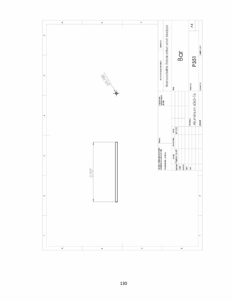
130

131

132
6 Unit

133
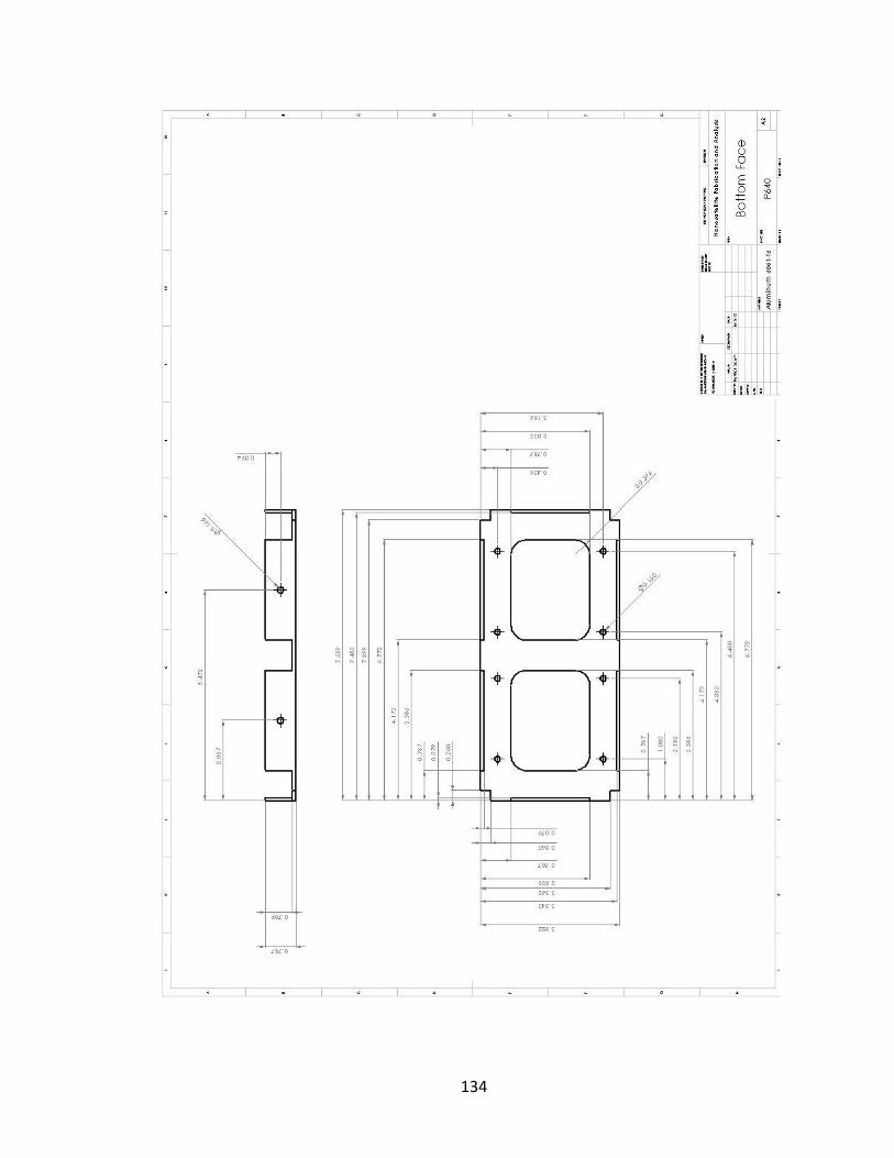
134

135

136

137

138
Assembly Tool

139
3 Unit Face Fixture

140

141
1 Unit Face Fixture

142

143
3 Unit Corner Bracket Fixture

144
APPENDIX III – PDS
REQUIREMENTS UNITS TARGET
Dimensions U “10x10x11.35 cm cube” 1-6
Weight kg 1.33 per U
Temperature °C -120 to 120
Sine Sweep Hz 20-2000
Random Vibration Grms 9.24
Cost US $ 400
Fasteners US $ 100
Parts US $ 100
Fixtures US $ 200
Materials
Frame Aluminum 6061-T6
Screws 316 Stainless Steal
Nuts 18-8 Stainless Steal

145
APPENDIX IV – TIMELINE

146

147

148

149
APPENDIX V – BUDGET SPREADSHEET
Item Name
Item Number Vendor Quantity Description Total Price
($)
Fasteners
N/A 90291A108 McMaster-
Carr 20
Nylon Tip 18-8 SS Socket Set Screw 4-40 Thread, 3/8"
Length
13.78
N/A 93190A542 McMaster-
Carr 25
Type 316 SS Fully Threaded Hex
Head Cap Screw 1/4"-20 Thread, 1"
Length
7.69
N/A 91735A104 McMaster-
Carr 50
Type 316 SS Pan Head Phillips
Machine Screw 4-40 Thread, 3/8"
Length
5.15
N/A 96439A140 McMaster-
Carr 50
18-8 Stainless Steel Clinch
Captive Nut 4-40 Thread Size, .056"
Minimum Panel Thickness
14.96
N/A 96877A198 McMaster-
Carr 50
18-8 SS 82 Deg Flat Head Phil
Machine Screw 4-40 Thread, 3/16" Length, Undercut
7.31
N/A 84985A45 McMaster-
Carr 4
Short Length SS Long-Nose Spring
Plunger 8-36 Thread, .5-1.5 lb
Nose Force
19.60

150
N/A 91125A621 McMaster-
Carr 4
18-8 SS Female Threaded Round
Standoff 1/4" OD, 7/16" Length, 6-32
Screw Size
6.12
N/A 91400A144 McMaster-
Carr 100
MIL Spec Pan Head Phillips
Machine Screw 300 Series, 6-32
Thread, 1/4" Length, MS 51957-
26, packs of 100
7.00
N/A 91099A125 McMaster-
Carr 100
18-8 SS Flat Undercut Head Phil Machine Screw 4-40
Thread, 3/16" Length, packs of
100
3.50
Total Price for Fasteners = 85.11
Tools for Fabrication
N/A 976-75622019 Enco 1 4-40 4" H2 2FL
Hertel HSS SP PT Plug Tap
35.21
N/A 3067A11 McMaster-
Carr 1
Corner-Rounding High-Speed Steel
End Mill 1/16" Radius, 1/4" Tip
Dia, 7/16" Mill Dia
31.92
N/A 8949A17 McMaster-
Carr 1
3/4" length of cut, 3/16" mill
diameter, 3/8" shank diameter
18.64
N/A S190 Starret 2 Jack Screw 108.00
Total Price for Fabrication Tools = 193.77

151
Materials
3X1 Unit Face
ASH6061/ 063 Metal
Supermarkets 4
3.75" X 12.75" X .063" Aluminum
sheet 6061 9.47
Corner Brackets
AF6061/ 34.05.05112
Metal Supermarkets
2 0.75" X 1.5" X 14" Aluminum Flat Bar
6061 18.82
Top and Bottom 1X1 Unit
Faces
AF6061/ 34.05.054
Metal Supermarkets
2 0.75" X 4" X 4"
Aluminum Flat Bar 6061
14.33
3X1 Unit Fixture
Base
AF6061/ 34.05.056
Metal Supermarkets
1 0.75" X 6" X 14"
Aluminum Flat Bar 6061
44.00
3X1 Unit Fixture
Top AF6061/ 386
Metal Supermarkets
1 0.375" X 6" X 14"
Aluminum Flat Bar 6061
17.35
1X1 Unit Fixture
Base AP6061/ 750
Metal Supermarkets
1 0.75" X 4.75" X 4.75"
Aluminum Plate 6061
15.54
1X1 Unit Fixture
Top AP6061/ 250
Metal Supermarkets
1 0.25"X 3" X 3"
Aluminum Plate 6061
2.05
Corner Bracket Fixture
AF6061/ 1144 Metal
Supermarkets 1
1.25" X 4" X 20" Aluminum Flat Bar
6061 84.30
Assembly Tool
AF6061/ 1126 Metal
Supermarkets 2
1.5" X 6" X 7.5" Aluminum Flat Bar
6061 59.76
Total Price for Materials = 265.62
Overall Price = 544.50

152
APPENDIX VI – SENIOR DESIGN CONFRENCE HANDOUT

153
Nanosatellite Fabrication and Analysis
Sam Harrison
Patrick Scott
Victor Zapien

154
Nanosatellites were first developed in 1955 to be used for communication. Surrey University was the first university to adopt the use of nanosatellites in 1981. By 1999, Stanford and Cal Poly created the CubeSat standard. It wasn’t till 2006 that NASA realized the potential of nanosatellites. Nanosatellites can be used for a variety of missions including deep space observation, biological research, earth observation and earthquake measurements. Santa Clara University has itself launched a couple nanosatellites.
The objective of our project is to develop an architecture for designing, analyzing and fabricating the structural frame of a nanosatellite. The goal is to be able to machine all the parts in house to lower cost and get experience in fabrication. Specialty tools are being designed and built to assist in the fabrication of the parts. This project is meant to be educational in terms of the knowledge gained as well as be beneficial to Santa Clara University by making it easier to produce nanosatellites. Our main focus is on designing and analyzing a 3 unit nanosatellite, but we also designed a 1 and 6 unit nanosatellite as well as a 3 unit nanosatellite with deployable solar panels. The nanosatellite needed to satisfy customer requirements such as being lightweight, durable and able to accommodate different mission capabilities. To ensure the durability of the nanosatellite frame we are performing modal, random vibration and thermal simulations.

155
Nanosatellite Fabrication and Analysis
Victor Zapien Patrick Scott Sam Harrison
Santa Clara University Students
Department of Mechanical Engineering
To Be Discussed
• Nanosatellite Overview and Background • Project Overview • Design requirements and customer needs • Nanosatellite designs and manufacturing • Analysis Simulation • Modal • Random vibration • Thermal
Nanosatellite Programs
• University nanosatellite programs • Educational
• Scientific research and advancements in technology. • SolidWorks, ANSYS, and MatLab
• Hands on experience • Fabrication
• Low cost
Key Terms
• 1 Unit = 10 x 10 x 11.35 cm • P-POD = Nanosatellite launch device • Pumpkin Incorporated = Nanosatellite company who made the 3 Unit nanosat here with us today. • ANSYS = Finite element software used for structural and thermal simulations. • SolidWorks = Computer aided design software used to design nanosat
• MatLab = Mathematical tool used for calculations • Modal Analysis = Analysis to calculate natural frequencies
SCHOOL OF ENGINEERING
Nanosatellite Background • All started back in 1955 with small satellites used for communication. • In 1981, Surrey University was the first university to launch a small satellite. • In 1999, the CubeSat standard was created by Stanford and Cal Poly.
• 2006, NASA realized nanosats full potential. • Deep space observation • Biological research • Earthquake measurements • Earth Observation
Problem Statement Development of an architecture for designing, analyzing, and fabricating the structural frame of a nanosatellite.

156
Project Overview
• 1, 3 and 6 unit nanosatellite • Design
• Meet customer needs and industry requirements. • Fabrication
• Using only the tools that the SCU machine shop provides.
• Testing • Thermal • Vibration
Customer Needs
• Meet testing specifications • Thermal • Vibration • Fit check • Lightweight, durable, optimize internal space. • Ability for cameras and sensors to see out of the
nanosat.
• Motherboard included • Deployable solar panels for more power which allows for bigger missions.
3 Unit Design
• 10 x 10 x 34.05 cm • Aluminum 6061 • 1.5875 mm side faces • 2 mm top and bottom faces. • 2 mm corner brackets.
• Open face design reduces weight and allows for customers to install cameras or sensors that need to see outside of the nanosat.
Design Requirements
• 1 Unit Nanosat • Natural frequency above • 10 x 10 x 11.35 cm 100 Hz. • 1.33 kg • 75 percent of nanosat rails • 3 Unit Nanosat must be in contact with P- • 10 x 10 x 34.05 cm POD rails. • 4 kg • Nanosat CG located within • 6 Unit Nanosat a 2 cm sphere that is • 10 x 20 x 34.05 cm centered at the geometric • 8 kg center.
1 Unit Design
• 10 x 10 x 11.35 cm • Aluminum 6061 • 1.5875 mm side faces • 2 mm top and bottom faces. • 2 mm corner brackets.
• Open face design reduces weight and allows for customers to install cameras or sensors that need to see outside of the nanosat.
3 Unit Design with Deployable Solar Panels
• 10 x 10 x 34.05 cm • Aluminum 6061 • 1.5875 mm side faces • 2 mm top and bottom faces. • 8.4582 mm corner brackets.
• Larger corner bracket may create enough room to allow for solar panel deployment. • Allows for missions that require • more power.

157
6 Unit Design
• 10 x 20 x 34.05 cm • Aluminum 6061 • 2.9058 mm side faces
• 2.9058 mm top and bottom faces. • 2.9058 mm corner brackets.
• Larger design allows for a bigger mission.
Circuit Board and Circuit Board Mounting
• Used on all 4 designs. •Attached directly to bottom face for easy installation and removal. • Santa Clara circuit board capable of all the necessary functions. • Has already been used successfully in space.
10 by 30 cm Face Fixture for Safe Machining
• Thin walls • Many pieces come loose as the faces are machined. • All 4 faces machined at once.
Manufacturing • Entire fabrication completed in Santa Clara Universities Machine
Shop. • Requires fixtures to machine delicate parts. • Requires assembly tool to ensure a good fit with P-POD • Circuit board will be attached directly to the bottom face. • Less than 500 dollars for everything.
Corner Bracket Fixture for Safe Machining
• Thin walls
• Piece is split in half when being machined. • 2 corner brackets machined at one time.
Tool for Assembly • Nanosat needs to be precise in its dimensions.
• Tools align brackets at the outmost dimension, which is the important one. • With a tool on either side holding the brackets in the desired location, the faces can be attached and the tools removed.

158
Fastening Our Assembly Together
• 3/16 inch 4-40 stainless steel undercut screw. • 4-40 stainless steel pem nut.
Modal Analysis - Determines vibration characteristics of a
structure such as natural frequencies corresponding mode shapes.
- Modal Analysis is a
pre-requisite for random vibration simulations and other dynamic simulations.
Random Vibration Simulation
Final 3 Unit Assembly Exploded
• 4x corner brackets • 4x 10 x 30 unit faces • 2x 10 x 10 unit faces • 1 motherboard
Random Vibration Simulation
- Large acceleration during random vibration can damage a structure. - Statistically analyzing the structures overall response to a random vibration environment. Input is a power spectral density, PSD. In this case acceleration spectrum density vs frequency.
- Interested in the root mean squared of the acceleration, Grms. - Special algorithm by Segalmam- Fulcher used to compute equivalent stress - Results follow a Gaussian Distribution
Thermal Analysis - Must calculate orbit path, local orientation, radiation view factors, solar position, and eclipse . - Heat sources - Direct Solar Radiation - Earth Infrared Radiation - Albedo - Internal Heat Generation

159
SatTherm
- Set of algorithms run in MatLab which can compute the orbit path, local orientation, and cumulative radiation absorbed by 6 sides of a satellite. Developed by Cassandra VanOutryve (SJSU) and NASA Ames. • Also has a finite difference algorithm which can calculate the transient temperature of each side of a satellite.
• Objective is to add to add code that would simulate an orbit orientation where a side is magnetically locked to the earth’s magnetic field.
SatTherm Orbit Simulation
Magnetically Locked Orbit
Conclusion
Development of an architecture for designing analyzing and fabricating the structural frame of a nanosatellite.
1, 3, 3 deployable, and 6 unit nanosats
Conducted Modal, Vibration, and Thermal Analysis
Thank you

160
APPENDIX VII – PROCEDURE
Below is a brief description of how all the fixtures and parts are machined in order to result in a functional 3 unit nanosatellite frame. It will be seen in the writing that exact locations of holes pockets and flanges are not discussed. All of the drawings in Appendix II can be referenced in order to properly machine all the parts. It is also very pertinent to communicate with Don MacCubbin when machining to ensure proper work. Some things done in our project could have been done slightly differently and Don would recommend these changes.
The overall fabrication consisted of 17 machined fixtures, parts and tools. Two parts made up the 1 unit fixture, one part for the corner bracket fixture and two parts for the 3 unit side face fixture. Then there is a top face and bottom face that come out of the 1 unit fixture, four corner brackets come out of the corner bracket fixture, two at a time, and four 3 unit side faces that are all machined at once in the 3 unit side face fixture. The last 2 machined components are the two assembly tools.
1 Unit Faces and Fixture
The first component done for this section was a bottom part of the 1 unit fixture. This was done by first bringing the aluminum 6061 block down to size. This is down to size based on the outside most dimensions in the x, y and z direction. Once this is done, it is time to pocket the block that is now down to size. The pocket is done so that the flanges seen below (1) actually connect all the way around the perimeter of the piece. Once the pocket is cut out down to the appropriate depth, all of the material that was left in the corner is taken out. The material in the corners is taken out down to the same depth of the pocket and the flanges left are the exact height and length of the flanges on the bottom and top faces. With the pocket cut out and the corners removed, the drill and tap holes (2) can be machined into the bottom on the fixture. With the bottom part of the 1 unit fixture complete, it is time to machine the top part for the 1 unit fixture.
Figure VII.1: 1 Unit Face Fixture Bottom
2 1

161
The top part of the fixture is made by once again bringing an aluminum 6061 block down to the appropriate size. Once, the block is down to size, the radii on the corners (1) can be machined one at a time. With all the radii machined, the holes (2) can be drilled into the center of the part. These holes are through holes for the drill and tap holes on the bottom part of the 1 unit fixture discussed above. With all of this done, the two parts that make up the 1 unit fixture are complete and ready for use.
Figure VII.2: 1 Unit Face Fixture Top
Before the top and bottom 1 unit faces go into the fixture, lots of machining has to take place. First, the block of aluminum is brought down to size. The next step is to machine out the four corner notches (1), one at each corner. With this complete, the mounting holes (2) for the captive nuts can be drilled. After this, the four holes in the bottom on the face (3) can be drilled and countersunk accordingly. The holes are countersunk in order to have the head of the chosen screw sit just below the surface of the face. With all the corners notched out, the captive nut mounting holes and motherboard through holes drilled it is time to pocket (4) the aluminum block. This is a four step process. The first pocket is 6. 35 mm larger all the way around the pocket seen that goes through the face. The pocket is more than 6.35 mm larger than the pocket that goes all the way through at the bottom left corner where it is smaller. This is done to accommodate the top part of the 1 unit fixture. So the first pocket is machined all the way down to the desired thickness of the face. When this is done, the pocket that goes all the way through can be machined out. The first step for this is machining out the bigger section of the through pocket. The second part is machining out the smaller section of the through pocket. The final step is run a perimeter cut that will clean up the two through pockets making one complete hole seen in the picture below.
2
1

162
At this point, the face is ready for the fixture. A picture of how the two parts of the fixture and the face go together can be seen below. Once it is fastened into the fixture the flanges (5) can be machined out. This is done by carefully removing all of the left over material without hitting the top part of the fixture and without removing too much material so that the flanges are too thin. If the drawings are followed to the numbers, there is no issue. When all of the extra material is removed, the screws can be removed from the fixture and the face can be taken out. When it comes out of the fixture it is completely done.
Figure VII.3: Bottom Face
The picture below is the top face to the 3 unit nanosatellite, while the face discussed above is the bottom face that holds the motherboard. Due to this there are two small differences that actually make the top face easier to machine. First, the four drill holes in the bottom of the face are not needed. Second, the three step process to remove the through pocket for the previous face is a one step process for this face. It is a simple pocket that goes all the way through.
Figure VII.4: Top Face
1
4 5
3
2
2

163
Below is the picture of how all three parts go together to order to remove the last bit of material around the flanges.
Figure VII.5: Example of 1 Unit Face Tool Use
3 Unit Faces and Fixture
To build the 3 unit side faces, a two part fixtures has to be made first. This is done by, once again bringing the aluminum down to the appropriate size for the part. Once it is brought down to size, it is time to pocket (1) the bottom fixture. The pocket leaves only three walls, which can be seen below in the picture. With the pocket complete the twelve drill and tap holes (2) can be machined. 6 are down the middle of the pocket and the other six run the perimeter of the part.
Figure VII.6: 3 Unit Face Bottom Tool
1
2

164
With the bottom part of the fixture complete, the top part has to be made so when the 4 side faces are inserted into the pocket of the bottom part of the fixture, they can be clamped down with the top face using the treaded holes machined into the bottom fixture. The top plate is very simple. The aluminum block is brought down to size and 12 through holes are machined into the plate so bolts can go through the top plate, and down into the bottom plate holding everything together.
Figure VII.7: 3 Unit Face Top Tool
With the fixtures ready, the faces have to be machined so they are ready for the fixture. Since the faces are 1.5 mm thick, they are all clamped together to make a piece strong enough to be put into a vice and machined. The first step, once the faces are clamped together is to bring them down to size. Once they four faces are down to size and clamped together, all of the drill holes can be implemented to the faces so when they come out of the fixtures they are complete. The first holes drilled (1) are mounting holes for the captive nuts. There are eight of them, four on each long side of the face. The next sets of holes are through holes (2) that go right through the cut outs seen in the face. There are two drill holes per pocket seen in the face, which amounts to six holes. These holes match up with the six threaded holes in the pocket of the bottom part of the fixture and the six holes in the top plate of the fixture. The last is a through hole that is countersunk (3) for the 4-40 undercut screws used. The countersink is to ensure the head of the screw is below the surface of the material. Since all the faces are clamped together this is a very delicate part. The through hole is drilled all the way through all four faces. The top face is them countersunk at the top through hole and the bottom through hole. The top face is then removed leaving only 3 faces. The now top face is countersunk at both locations and then removed as well. This is continued till all the faces are done. It is very important to loosen the vice pressure so when doing the final face in the vice it will not bend or deform.
2
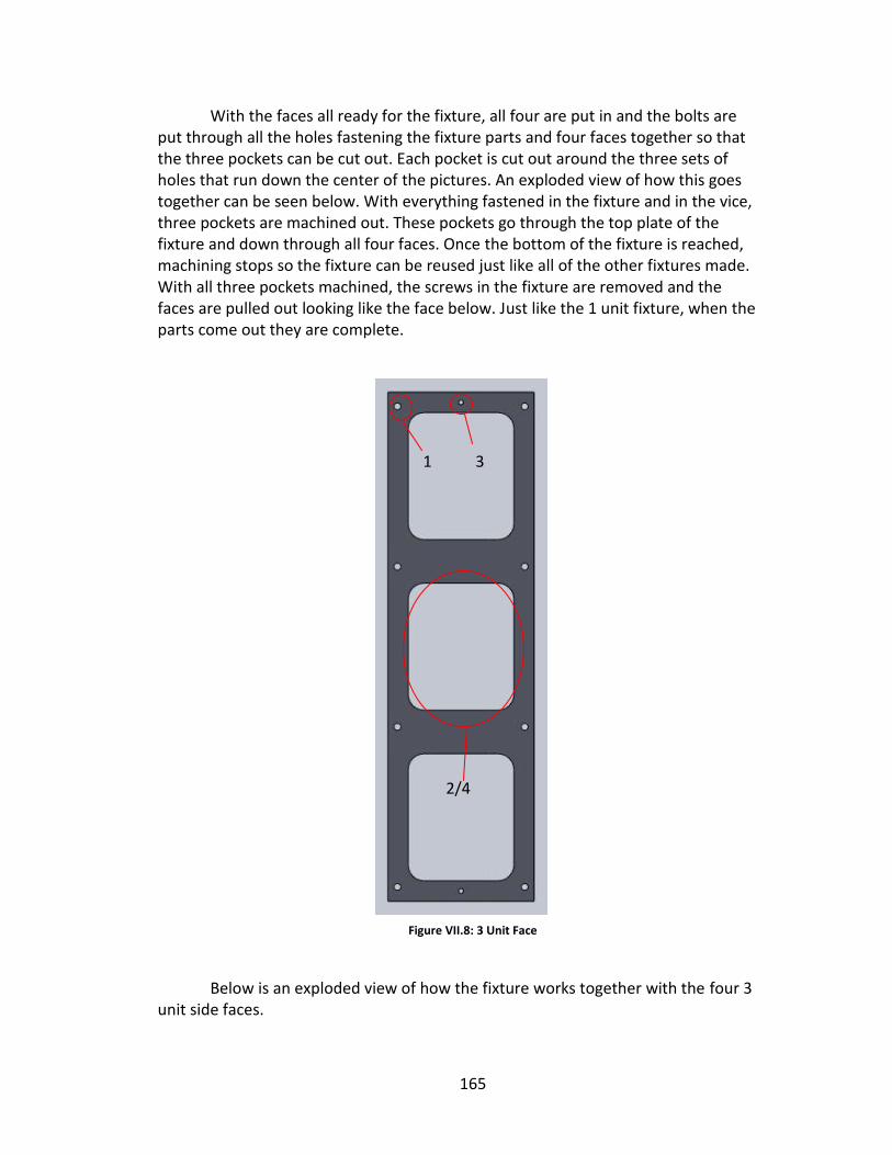
165
With the faces all ready for the fixture, all four are put in and the bolts are put through all the holes fastening the fixture parts and four faces together so that the three pockets can be cut out. Each pocket is cut out around the three sets of holes that run down the center of the pictures. An exploded view of how this goes together can be seen below. With everything fastened in the fixture and in the vice, three pockets are machined out. These pockets go through the top plate of the fixture and down through all four faces. Once the bottom of the fixture is reached, machining stops so the fixture can be reused just like all of the other fixtures made. With all three pockets machined, the screws in the fixture are removed and the faces are pulled out looking like the face below. Just like the 1 unit fixture, when the parts come out they are complete.
Figure VII.8: 3 Unit Face
Below is an exploded view of how the fixture works together with the four 3 unit side faces.
2/4
1 3
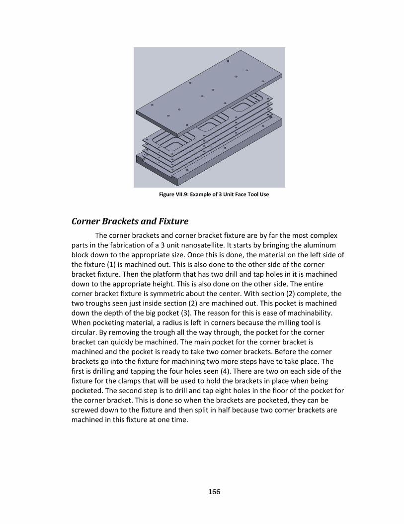
166
Figure VII.9: Example of 3 Unit Face Tool Use
Corner Brackets and Fixture
The corner brackets and corner bracket fixture are by far the most complex parts in the fabrication of a 3 unit nanosatellite. It starts by bringing the aluminum block down to the appropriate size. Once this is done, the material on the left side of the fixture (1) is machined out. This is also done to the other side of the corner bracket fixture. Then the platform that has two drill and tap holes in it is machined down to the appropriate height. This is also done on the other side. The entire corner bracket fixture is symmetric about the center. With section (2) complete, the two troughs seen just inside section (2) are machined out. This pocket is machined down the depth of the big pocket (3). The reason for this is ease of machinability. When pocketing material, a radius is left in corners because the milling tool is circular. By removing the trough all the way through, the pocket for the corner bracket can quickly be machined. The main pocket for the corner bracket is machined and the pocket is ready to take two corner brackets. Before the corner brackets go into the fixture for machining two more steps have to take place. The first is drilling and tapping the four holes seen (4). There are two on each side of the fixture for the clamps that will be used to hold the brackets in place when being pocketed. The second step is to drill and tap eight holes in the floor of the pocket for the corner bracket. This is done so when the brackets are pocketed, they can be screwed down to the fixture and then split in half because two corner brackets are machined in this fixture at one time.

167
Figure VII.10: Corner Bracket Tool
With the corner bracket fixture ready, the corner brackets have to be machined. Remember 2 corner brackets are machined at once and come from one piece. They are attached alone the long side and split into two pieces once in the fixture. Getting ready for the fixture, the aluminum was once again brought down to the correct size. Once the piece is the correct size, two external radii are machined into the piece of aluminum. The radii run the long length of the piece and will be in the bottom of the fixture when it is put in. After the radii are complete, one side of the cubes (1) is machined out. After this, all the holes are drilled and countersunk in their appropriate locations. Again, the holes (2) are countersunk so that the screw heads are below the surface of the material. With one side of the cubes cut out, the radii machined into the piece and the holes drilled and countersunk, the pieces is ready for the fixture.
The piece is put into the fixture with the radii down and drill holes down and on the sides. These parts cannot be seen when it is in the fixture because the top is what is being pocketed so all the previous work is facing down. The cubes are then clamped to the fixture, which can be seen in the assembly below. With the piece fastened to the fixture, the piece is pocketed down to the appropriate depth using a big milling tool to save time. After the majority of the pocket is done a small milling tool is used to clean up the corners of the pocket as best as possible. At this point the clamps are removed and the brackets are fastened to the fixture using the eight holes drilled and tapped in the bottom of the fixture. That same tool is then used to finish the cubes (4) and then the piece is split down the middle so two brackets are present. However, we are not done yet. Just like before inside corners have a radius due to the milling tool. To eliminate the extra material, the brackets switch sides in the fixture put the side that was down on the side of the fixture and the side that was on the side of the fixture down onto the base of the pocket. This will allow the team to machine out the material left over in the vertical direction from the milling tool. Once this material is cleaned up two brackets are done. This is repeated for the other brackets.
1
3
4
2

168
Figure VII.11: Corner Bracket
Below is a half exploded view of everything together to show how the brackets look in the fixture and how the clamps hold the parts in place during machining.
Figure VII.12: Example of Corner Bracket Tool Use
2
3
1
4

169
Assembly Tool
The final parts machined are the two assembly tools. These were made by first bring the aluminum block down to size. The next step was removing all the material except the big base and the four cubes that protrude from the base (1). Once this is done each cube needs to be handled separately. Working with one cube, the first step is to drill out the corners of the inside pocket that is going to be made. The reason for drilling the four corners out of each cube is because the milling tool leaves a radius when pocketing material. To get the corners of the cubes on the corner brackets to fit in, the corners must be drilled out before the pocket is made. With the corners drilled out it is time to pocket each of the four cubes down to the appropriate depth (2). With this done, the holes (3) can be drilled and tapped to hold the nylon tip set screws. This is repeated for the other assembly tool.
Figure VII.13: Assembly Tool
2
1
3

