This document is downloaded at: 2018-08-22T06:07:25Z

Title Study on Simplified Speed Sensorless Vector Control Systems forInduction Motors

Author(s) Mangindaan, Glanny Martial Christiaan

Citation Nagasaki University (長崎大学), 博士(工学) (2015-03-20)

Issue Date 2015-03-20

URL http://hdl.handle.net/10069/35214

Right

NAOSITE: Nagasaki University's Academic Output SITE

http://naosite.lb.nagasaki-u.ac.jp

Study on Simplified Speed Sensorless

Vector Control Systems for Induction Motors

February 2015

Graduate School of Engineering

Nagasaki University

Glanny Martial Christiaan Mangindaan

CONTENTS

Chapter 1 Introduction 1.1 Background ............................................................. 1

1.2 Content of Chapters ................................................ 8

Chapter 2 Models of Induction Motor 2.1 Space Vector Representation of Induction Motor .... 10

2.2 d – q Model ............................................................ 19

2.3 Electromagnetic Torque ........................................ 23

2.4 Non – linear State Equation ................................... 25

2.5 Linear State Equation ............................................ 26

Chapter 3 Speed Sensorless Vector Control Systems 3.1 Proposed System A ................................................ 28

3.1.1 Block Diagram of System A ............................ 28

3.1.2 Description of System ..................................... 32

3.1.3 Steady – state Analysis .................................... 35

3.1.4 Linear Model ................................................... 39

3.2 Proposed System B ................................................ 44

3.2.1 Block Diagram of System B ............................ 44

3.2.2 Description of System ..................................... 46

3.2.3 Steady – state Analysis .................................... 47

3.2.4 Linear Model ................................................... 48

3.3 Gain Selection of Controller .................................. 51

3.3.1 Current Controller ........................................... 51

3.3.2 Speed Controller .............................................. 53

Chapter 4 Simulation and Experimental Results 4.1 Experimental System ............................................. 55

4.1.1 Microcomputer Control System ...................... 55

4.1.2 Parameters of System ...................................... 59

4.1.3 Experimental IM – DCM System .................... 62

4.2 System Stability ..................................................... 66

4.3 Simulation Results ................................................. 75

4.4 Experimental Results ............................................. 84

Chapter 5 Conclusion ................................................ 96

References ......................................................................... 99

1

Chapter 1

Introduction

1.1 Background

The induction motors (IM) are very common and easy to find, because

it is low in price and robust. Those are used in industrial applications such as

electric train, pump, fan, machine tools, grinders, conveyors and home

utilizations. Conventionally, till the last of the twentieth century, the induction

motors are operated at a single speed, which is determined by the frequency

of main voltage and the number of poles. Typically, they were operated from

fixed-frequency sources 50 Hz or 60 Hz in most cases.

To control the IM speed, a variable-frequency source is required, and

such kind source did not readily exist. Thus, applications necessitating

variable speed were serviced by direct-current motors (DCM). So, controlling

the speed of IM is more difficult than controlling the speed of DCM, because

the relationship between the motor current and the resulting torque is not

linear for IM.

The availability of solid-state power switches, development of power

electronics and microelectronics change this scheme hugely. Recently

developed solid-state power device such as insulated gate bipolar transistors

(IGBT), metal-oxide semiconductor field-effect transistors (MOSFET) are

applied to many favorable switches with wide range power ratings and

switching frequency that make them suitable candidates for variable-

frequency generation. Now the power electronics are capable for supplying

the variable voltage/current, or frequency drive to realize variable-speed

2

performance for IM. About the microelectronics, a digital signal processor

(DSP) has been developed. By using C language, control algorithm is

programed and realized without adding hardware.

Recently, to reduce the pollution problem in urban area and the

availability of fossil fuel, the electric car is getting attention; but because of

the limited performance of the battery as an energy storage, it would take

considerable time to use pure electric car commonly. Many of electric cars

use interior permanent magnet synchronous motor (IPMSM) from the

viewpoint of motor efficiency. However, it is interesting that the Tesla

Company uses the IM for electric car.

According to the development of pulse width modulation (PWM)

inverter, the constant volt per hertz (V/f) control is applied at first as variable-

speed control method for IM. However, the constant V/f control cannot

control torque instantaneously. On the other hand, the vector control (or field

oriented control) can control torque instantaneously and control speed of IM

quickly. In order to realize vector control, the information of rotor flux angle

is indispensable. In order to estimate the rotor flux angle, the angular

frequency is computed by adding the rotor speed to the slip angular frequency.

The slip angular frequency is obtained from a current model of IM by

assuming that the q – axis flux becomes zero. The rotor flux angle is obtained

by integrating the angular frequency. Many researches for rotor resistance

identification are reported to compute accurate the slip frequency [10], [16],

[20], [21].

By using the rotor flux angle, the three phases currents are

transformed to two-axis (d – q) currents. In general, the d – axis is selected as

the direction of rotor flux vector. Therefore, the d – axis current is

proportional to the magnitude of the rotor flux. The electromagnetic torque is

proportional to the product of d – and q – axis currents. By controlling the d –

3

and q – axis currents quickly, the torque is produced instantaneously without

transient. In general, this currents control are achieved by PI control through

voltage control by PWM inverter. At steady – state the d and q variables

become constant. The d and q currents correspond to the field current and the

armature current of DCM respectively.

However, the use of such direct speed sensor induces additional

electronics, extra wiring, extra space, frequent maintenance, careful mounting

and default probability. The use of speed sensor has problems occurred,

mainly in harsh environment. Moreover, the speed sensor is sensitive for

electromagnetic noise in hostile environments and has a limited temperature

range. To avoid mechanical sensor (speed and position) of IM, several

methods called sensorless vector control is used. In order to simplify the

hardware, the speed sensorless vector control is studied and applied in

practical uses.

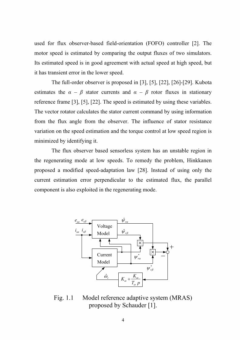
In order to improve the performance of induction motor control

without speed sensor, many model reference adaptive system (MRAS) based

methods are studied. Representative speed estimation is MRAS based method

proposed by Schauder [1]. Figure 1.1 shows the two independent simulators

are constructed to estimate the component of the rotor flux vector. Hence,

voltage model does not involve the quantity of rotor electrical-angular speed,

this model is used as a reference model, and current model which does

involve rotor electrical-angular speed is used as an adjustable model. The

errors between the states of the two models are used to derive a proper

adaptation mechanism that generates the estimation of rotor electrical-angular

speed for the adjustable model. The terminal currents and voltages are

measured and transformed to α – β variables. However, the vector control

system using MRAS speed estimate is composed independently. Therefore,

the system becomes complex. The speed estimation using flux simulator is

4

used for flux observer-based field-orientation (FOFO) controller [2]. The

motor speed is estimated by comparing the output fluxes of two simulators.

Its estimated speed is in good agreement with actual speed at high speed, but

it has transient error in the lower speed.

The full-order observer is proposed in [3], [5], [22], [26]-[29]. Kubota

estimates the α – β stator currents and α – β rotor fluxes in stationary

reference frame [3], [5], [22]. The speed is estimated by using these variables.

The vector rotator calculates the stator current command by using information

from the flux angle from the observer. The influence of stator resistance

variation on the speed estimation and the torque control at low speed region is

minimized by identifying it.

The flux observer based sensorless system has an unstable region in

the regenerating mode at low speeds. To remedy the problem, Hinkkanen

proposed a modified speed-adaptation law [28]. Instead of using only the

current estimation error perpendicular to the estimated flux, the parallel

component is also exploited in the regenerating mode.

VoltageModel

*r

*r

ˆ r

ˆ r

CurrentModel

KKT p

se se

si si

ˆr

Fig. 1.1 Model reference adaptive system (MRAS)

proposed by Schauder [1].

5

Design strategy of both observer gains and speed estimation gains for

an adaptive full-order observer based sensorless system is necessary issue to

assure the stability and the tracking performance. Suwankawin proposed a

design of observer gains to achieve the stability over the whole operation

especially in the low-speed region, including the regenerating operation [26].

The speed estimation gains are designed by considering the ramp response of

the speed estimator. There is still an unstable region of experimental result in

plugging region.

Tursini proposed an adaptive speed-sensorless field-oriented control

of an induction motor, based on a sliding-mode observer [24]. Using the

voltage equation, the observer computes the stator current and the rotor fluxes

in α – β stationary reference frame. In the case of sliding-mode observer, it is

considered that the observer gains are very large. The rotor speed estimation

is obtained by using relation with a Lyapunov function. The system

performance with different observer gains and the influence of the motor

parameters deviations are shown. Sliding-mode full-order observer also are

reported in [25], [30].

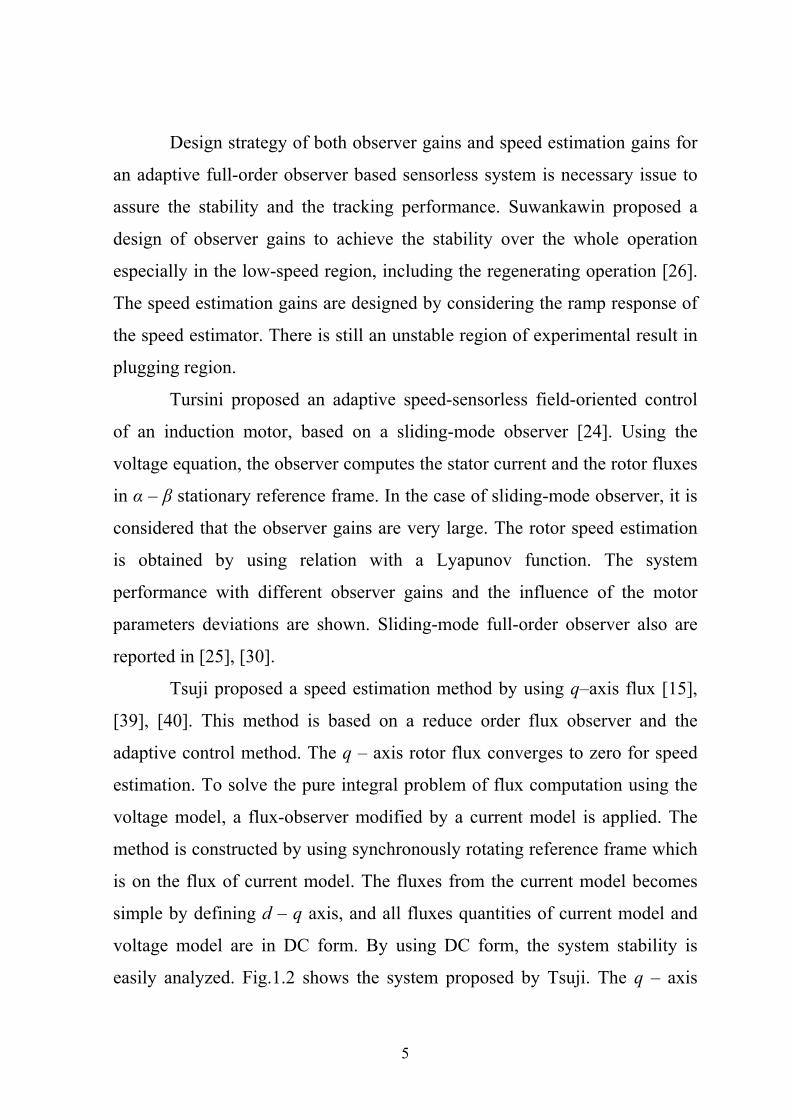
Tsuji proposed a speed estimation method by using q–axis flux [15],

[39], [40]. This method is based on a reduce order flux observer and the

adaptive control method. The q – axis rotor flux converges to zero for speed

estimation. To solve the pure integral problem of flux computation using the

voltage model, a flux-observer modified by a current model is applied. The

method is constructed by using synchronously rotating reference frame which

is on the flux of current model. The fluxes from the current model becomes

simple by defining d – q axis, and all fluxes quantities of current model and

voltage model are in DC form. By using DC form, the system stability is

easily analyzed. Fig.1.2 shows the system proposed by Tsuji. The q – axis

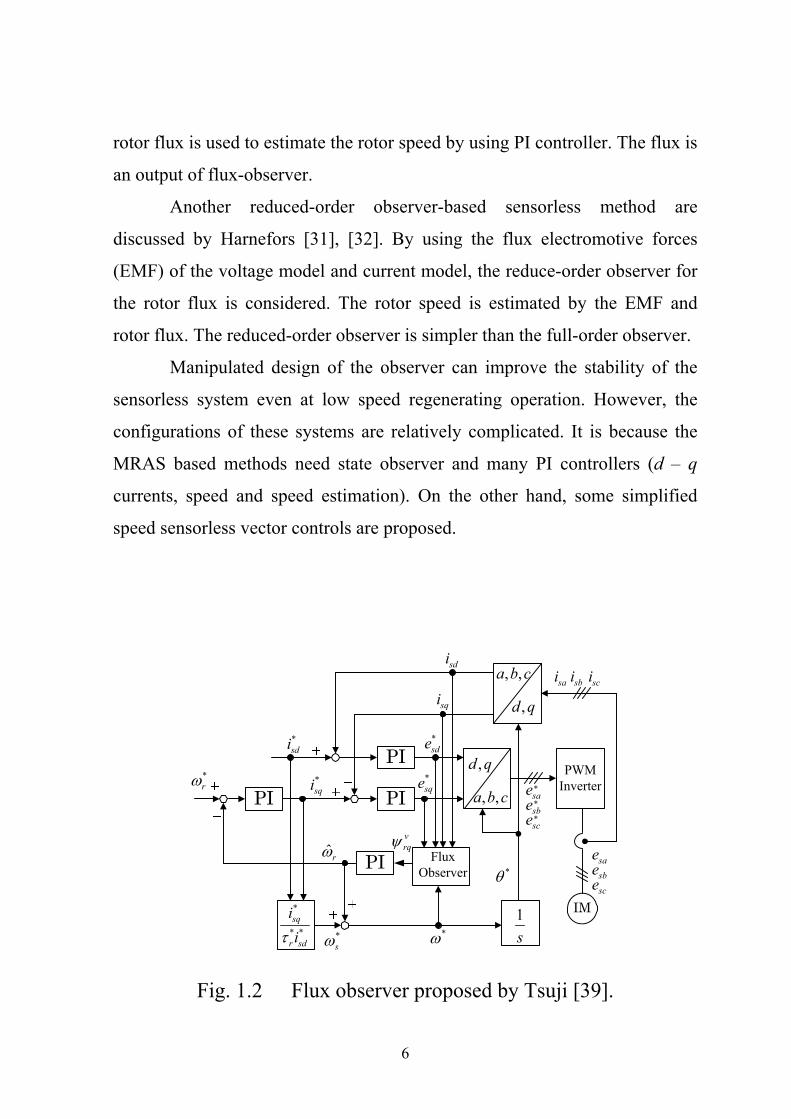
6

rotor flux is used to estimate the rotor speed by using PI controller. The flux is

an output of flux-observer.

Another reduced-order observer-based sensorless method are

discussed by Harnefors [31], [32]. By using the flux electromotive forces

(EMF) of the voltage model and current model, the reduce-order observer for

the rotor flux is considered. The rotor speed is estimated by the EMF and

rotor flux. The reduced-order observer is simpler than the full-order observer.

Manipulated design of the observer can improve the stability of the

sensorless system even at low speed regenerating operation. However, the

configurations of these systems are relatively complicated. It is because the

MRAS based methods need state observer and many PI controllers (d – q

currents, speed and speed estimation). On the other hand, some simplified

speed sensorless vector controls are proposed.

IM

PI*r

*sdi

*sqi

PI

PI

sdi

sqi

*sde

*sqe

sbesae

sce

saesbesce

, ,a b csai sbi sci

*

* *sq

r sd

ii

ˆr

*s

1s*

*

vrq

,d q

, ,a b c

,d q PWMInverter

PI FluxObserver

*

*

*

Fig. 1.2 Flux observer proposed by Tsuji [39].

7

Simplifying the system configuration by removing the current

regulators is proposed [33], and the stability is improved by adding a flux-

stabilizing controller using derivative of magnetic current [34]. However,

these papers have no information about the stability of regenerating mode. A

sensorless method using the induced d – axis and q – axis voltage obtained by

a voltage model has been proposed [35], and a similar method is applied to

railway vehicle traction [36]. However, the stable region is not clear in these

papers. Furthermore, a primary flux control method are proposed in [17], [37]

and the stability is improved at regenerating mode [38]. Simple method of

stator – flux orientation is proposed in [23]. Some survey papers for IM

sensorless control systems are reported in [4], [9], [18]. Parameter estimation

of stator and rotor resistances are also important problem for the sensorless

systems [6], [11].

In this thesis, a new simplified speed-sensorless vector control method

of IM based on q – axis rotor flux is proposed [41] – [44]. A flux vector is

obtained from voltage model, in which the derivative term is neglected. A

flux angle of a current model must be aligned with the flux angle of voltage

model. Since the output voltage of d – axis PI current controller is used for the

flux angle estimation and speed control (q–axis voltage control), the system is

simplified and stabilized at regenerating mode [41]. In conventional

simplified methods, this scheme is not reported. A linear model of the

proposed system in the state space equation is obtained to study the system

stability by showing root loci. By virtue of the stability analysis, we can

design the parameters of controller. The nonlinear simulation and

experimental results of the proposed system show stable transient responses in

both motoring and regenerating modes [43]. In order to improve the system

stability at plugging region, a PI speed controller is studied instead of original

I (integral) controller [42]. Furthermore, a simplified sensorless system that

8

uses a PI q– axis current controller and estimates the rotor speed is studied

and compared [44].

1.2 Contents of Chapters

This thesis is divided into five chapters with the arrangement:

In chapter 1, the background and the purpose of this research are

explained and the contents of chapters are specified.

Chapter 2 describes a space vector representation of induction motor.

A three-phase mathematical model of induction motor is transformed to a d –

q model by using two-axis theory. This chapter introduces a non-linear model

and a linear model of induction motor. The linear model of induction motor is

derived by considering small perturbations at a steady state operating point.

In chapter 3, new simplified speed-sensorless vector control methods

of IM based on rotor flux linkage are proposed . The two simplified sensorless

systems are called as system A and system B. The main difference is the

presence (in system A) or the absence (in system B) of q – axis PI current

controller. In system A, the angular frequency of rotor flux is estimated to

bring q–axis flux to zero by using PI controller. The q – axis flux is obtained

by the output of d – axis PI current controller with a non-interference control.

The rotor speed is computed by subtracting a slip speed from the angular

frequency. Flux angle is obtained by integrating the angular frequency. When

q – axis flux is larger (smaller) than zero and rotor flux is leading (lagging)

than d – axis, the controller must increase (decrease) the value of flux

frequency. In system B, the computation of q – axis flux is as same as the

system A. The angular frequency of rotor flux is computed by adding the q –

axis flux to the speed command. The q – axis flux is also used to control the

rotor speed, by adjusting the q – axis voltage. Non-linear models are derived

9

in both proposed systems A and B. From these non-linear models, linear

models of the systems are derived in state space equations. The selection of PI

current and speed controllers gains are outlined.

Chapter 4 demonstrates systems stability by showing the root loci

obtained by the linear models, the transient responses of simulation results

and the stable regions. The performance of both systems A and B are

compared by using linear models and non-linear models. Transient responses

of linear and non-linear models are computed and compared. Since both

responses are almost same around a steady state operating point, the validity

of the linear models are confirmed. By using the proposed methods, not only

the motoring operation but also the low speed regenerating operation can be

stabilized. Quick torque and speed responses of nonlinear models are obtained

in both systems A and B. A digital signal processor based PWM inverter fed

IM system is equipped and tested. It is confirmed that the experimental results

are very close to those of simulation. Therefore, the effectiveness of the

proposed methods are also demonstrated experimentally. It is considered that

the system B is superior to the system A because its simple structure.

Chapter 5 is the conclusions presented in this thesis.

10

Chapter 2

Models of Induction Motor

2.1 Space Vector Representation of Induction Motor

For convenience of proposed systems analysis, the models of IM are

outlined. In order to analyze the IM, it must be embodied in three-phase

mathematical model. From three-phase model, the IM is simplified into two-

phase by using the two-axis transformation [12], [13], [14].

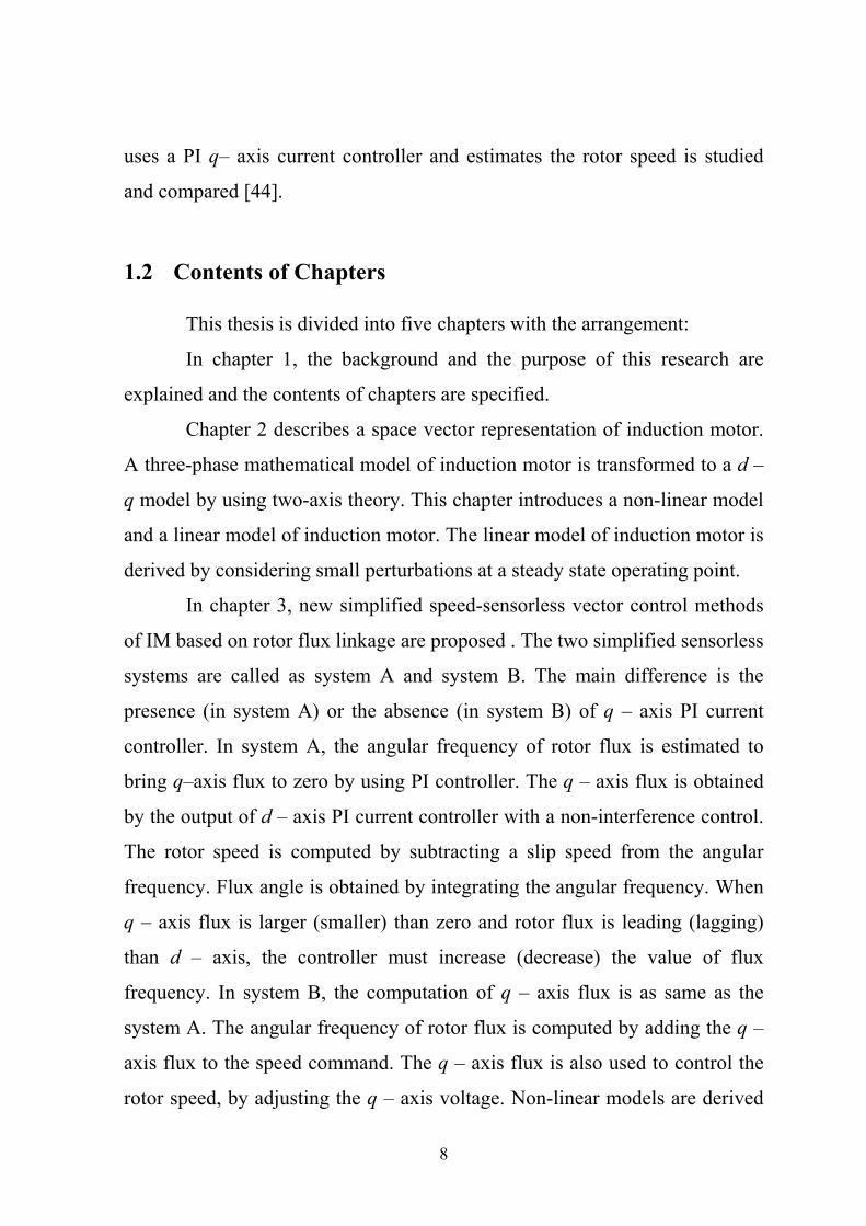
To show windings configuration and to calculate inductances, the

cross-section of simplified three-phase IM with two-poles is shown in Fig.2.1.

The winding configurations are assumed the same to each phases of both the

stator and the rotor. The winding of three-phase IM is separated by 120

electrical degrees with respect to each other as shown by the coils a – *a ,b– *b

and,c – *c .

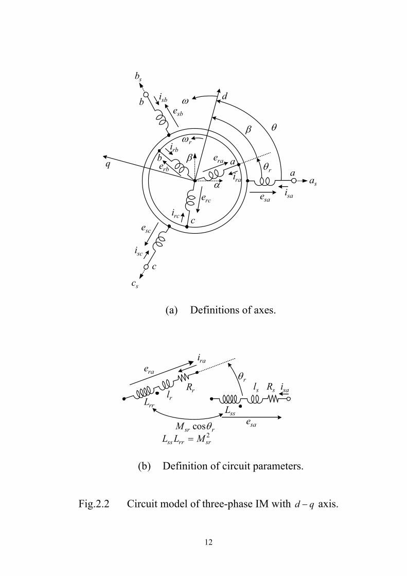
Fig.2.2 shows a circuit model of the three-phase IM with two-poles.

An equivalent three-phase winding is used in case of short-circuited squirrel-

cage rotor. The stator and rotor windings are wye connected. The sa , sb and

sc mean the axes of stator a , b and c phase winding respectively. The angle

r is an angular displacement of a -phase rotor winding axis from the axis sa .

By using the rotational angular velocity r , the angle r is expressed as

0

0t

r r rdt ......................................................... (2.1)

11

The stator winding of IM is fundamentally the same as for a

synchronous motor. In the below equations, the subscript s denotes variables

and parameters associated with the stator circuits, and the subscript r denotes

variables and parameters associated with the rotor circuits.

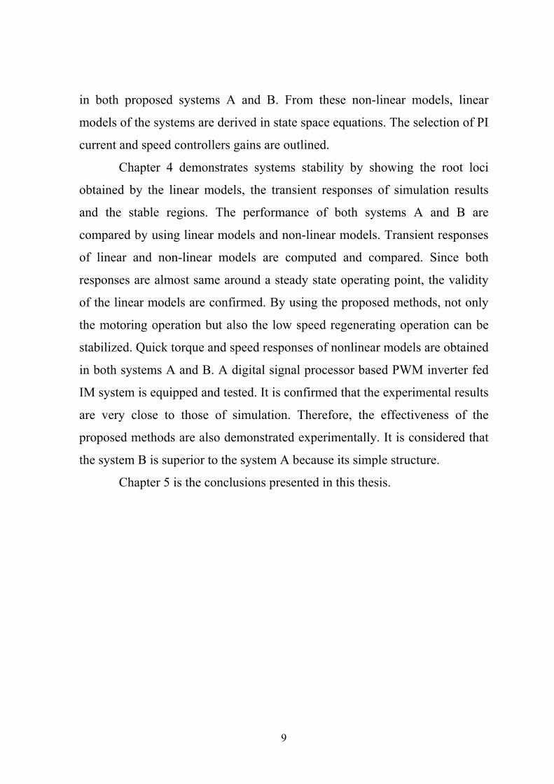
In Fig.2.2 (b), the leakage inductance at stator and rotor windings are

sl and rl respectively. The mutual inductances srM has the relation with self-

inductances ssL and rrL as follows:

2

ss rr srL L M ..................................................................... (2.2)

a

a

b bcc

*a

*b*c

*a

*b *c120

Fig. 2.1 Three-phase stator and rotor windings of IM.

12

sbesbi

saerce

rae

scerci

rai

sai

sci

rbi

a

b

c

d

q

r

rbe

r

ab

c

sa

sb

sc (a) Definitions of axes.

sRsl sai

sae

r

ssL

cossr rM 2

ss rr srL L M

rRrl

raerai

rrL

(b) Definition of circuit parameters.

Fig.2.2 Circuit model of three-phase IM with d q axis.

13

The mutual inductance between stator and rotor changes when the

rotor moves by the angle r . The rotor a -phase current rai generates flux in

the stator a -phase winding as shown in Fig2.3. If 0r , all flux by rai passes

ssL and the mutual inductance is srM . As the cosine component of the flux by

rai passes ssL , the mutual inductance becomes cossr rM . The flux linkages in

three-phase windings of the stator and the rotor are defined as sa , sb , sc

and ra , rb , rc respectively. By considering the cosine component of the

angle of the winding, we can obtain the flux linkages of sa , sb , sc , ra ,

rb , rc as follows:

/ 2 / 2/ 2 / 2/ 2 / 2

sa s ss ss ss sa

sb ss s ss ss sb

sc ss ss s ss sc

l L L L iL l L L iL L l L i

2 2cos cos cos3 3

2 2cos cos cos3 32 2cos cos cos3 3

r r r

ra

sr r r r rb

rc

r r r

iM i

i

..... (2.3)

14

/ 2 / 2/ 2 / 2/ 2 / 2

ra rar rr rr rr

rb rr r rr rr rb

rr rr r rrrc rc

il L L LL l L L iL L l L i

2 2cos cos cos3 3

2 2cos cos cos3 32 2cos cos cos3 3

r r r

sa

sr r r r sb

sc

r r r

iM i

i

..... (2.4)

By using the flux linkages, the following voltage equations are

obtained for stator and rotor windings.

sa sa sa

sb s sb sb

sc sc sc

e ie R i pe i

.................................................. (2.5)

ra ra ra

rb r rb rb

rc rc rc

e ie R i pe i

.................................................. (2.6)

where, p means d dt , sR and rR is stator resistance and rotor resistance

respectively.

rai ssLrrL

All flux by passes ra ssi L

Mutual inductance srM

0r

rair

ssLrrL

cos component of flux by passes

r

ra ssi L

Mutual inductance cos0 2

sr r

r

M

Fig.2.3 Mutual inductance of windings.

15

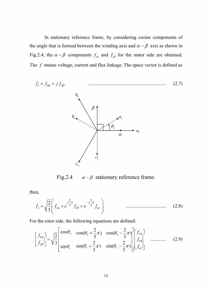
In stationary reference frame, by considering cosine components of

the angle that is formed between the winding axis and axis as shown in

Fig.2.4, the components sf and sf for the stator side are obtained.

The f means voltage, current and flux linkage. The space vector is defined as

s s sf f j f ................................................................ (2.7)

sa

ra

sb

r

rb

rcsc

Fig.2.4 stationary reference frame.

then, 2 23 32

3j j

s sa sb scf f e f e f

................................. (2.8)

For the rotor side, the following equations are defined:

2 2cos cos( ) cos( )2 3 3

2 23 sin( ) sin( )sin3 3

r rar rr

rbr

r rr rc

ff

ff

f

............. (2.9)

16

By using rf and rf , the space vector is defined as

r r rf f j f ............................................................... (2.10)

then, 2 23 32

3r

j jjr ra rb rcf e f e f e f

.......................... (2.11)

The space vector of stator voltage is expressed as 2 23 32 ( )

3j j

s sa sb sce e e e e e

................................... (2.12)

From (2.5), we have

s s s se R i p ............................................................... (2.13)

The stator flux linkage is computed from (2.3) as 2 23 32 ( )

3j j

s sa sb sce e

2 23 3

2 23 3

2 23 3

2 23 3

22 3

2 cos3

2 2cos3 3

2 2cos3 3

j jsss ss s sb sc sa sc sa sb

j jsr r ra rb rc

j jsr r rb rc ra

j jsr r rc r

s

a rb

Ll L i i i e i i e i i

M i e i e i

M i e i e i

M i e i e i

17

By using sa sb sci i i , sb sc sai i i and sc sa sbi i i , we have

2 23 3

32

2 2cos cos cos3 3

r

s s ss s

j jjj r j rsr r r r r r r

l L i

M i e i e e i e e

3 32 2

r rj js ss s ss r rl L i M i e e

3 3( )2 2s ss s ss r rl L i M i .............................................. (2.14)

By setting 32s ss sL L l and 3

2 srM M , (2.14) can be written as:

s s s rL i M i ............................................................... (2.15)

Substituting (2.15) into (2.13), we have

s s s s re R p L i p M i ............................................... (2.16)

The space vector of rotor is expressed as follows: 2 23 32

3r

j jjr ra rb rce e e e e e e

............................ (2.17)

From (2.6), we have 2 23 32

3r

j jjr r r ra rb rce R i e p e e

...................... (2.18)

hence,

r rj jr r r re R i e p e ............................................. (2.19)

18

The space vector of the rotor flux linkage is computed from (2.4) as

2 23 32

3r

j jjr ra rb rce e e

2 23 3

2 23 3

3 2 cos2 3

2cos3

rj jj

r rr r sr r sa sb sc

j jr

r

sb sc sa

l L i e M i e i e i

i e i e i

2 23 32cos

3j j

r sc sa br si e i e i

......................... (2.20)

therefore,

3 32 2r r rr r sr sl L i M i

........................................... (2.21)

By setting 32r rr rL L l , the rotor flux linkage is expressed as

r r r sL i M i ............................................................... (2.22)

From (2.19), we have

( ) ( )r r r r r r r se R i p j L i p j M i ............................... (2.23)

The space vector equation of IM from equations (2.16) and (2.23) is

expressed as

( ) ( )s s s s

r r r r r r

e R L p Mp ie p j M R p j L i

........................... (2.24)

19

The voltages se and re in (2.24) are divided into real and imaginary

parts to have stationary reference model as

0 00 0

s ss s

s ss s

r rr r r r r

r rr r r r r

e iR L p Mpe iR L p Mpe iMp M R L p Le iM Mp L R L p

............. (2.25)

2.2 d – q Model

We consider a rotating d q axis shown in Fig.2.5. Where, is the

angle between axis and d axis. The d axis rotates at an arbitrary

angular velocity . Then, can be expressed by the following equation:

0(0)

tdt ............................................................ (2.26)

The stationary reference frame quantities are transformed into

rotating reference frame quantities using d q transformation as follows:

j jsdq s s sf e f j f e f

.................................... (2.27)

j

rdq rf e f .................................................................... (2.28)

20

sa

q

sf

sf

s dfs qf

d

cossf

cossf sinsf

sinsf

cos sinje j jsdq s s

js

f f j f e

f e

sf

Fig.2.5 Reference frame transformation from to d q .

Hence, the transformation of reference frame from to d q

axis can be expressed as

cos sinsin cos

sd s

sq s

f ff f

........................................ (2.29)

From (2.16) and (2.27), we have

jsdq s

js s s r

e e e

e R p L i p M i

j j j js sdq s sdq rdqsdqe R i e L p e i e M p e i

s sdq s sdq s sdq rdq rdsdq qR i L pi j L i M p i j M pie .......... (2.30)

21

From (2.23) and (2.28), we have

jrdq r

jr s r r r r

e e e

e p j M i R p j L i

j j j j j jr rdq sdq r sdq

j j j jr rdq

rdq

r r rdq

e R e i e M p e i e j M e i

e L p e i e j L i

e

e

r rdq sdqr sdq r sdqdq R i M pi j M i j Me i

r rdq r rdq r rrdq rdqL pi j L Le i j i .................................. (2.31)

The voltage equations of (2.30) and (2.31) can be written in matrix

form as

sdq sdqs s s

rdq rdqr r r r r

e iR L p j L Mp j Me iMp j M R L p j L

...... (2.32)

Hence, sdqe and rdqe can be divided into real and imaginary parts as

follows:

sd sds s s

sq sqs s s

rd rdr r r r r

rq rqr r r r r

e iR L p L Mp Me iL R L p M Mpe iMp M R L p Le iM Mp L R L p

............ (2.33)

The relation between sdqf and three-phase variables can be expressed

as 2 23 32

3j jj

sdq sa sb scf e f e f e f

........................... (2.34)

22

Therefore, we have

2 2cos cos cos3 32

3 2 2sin sin sin3 3

sasd

sbsq

sc

ff

ff

f

........ (2.35)

The relation between rdqf and three-phase variables can be expressed

as 2 23 32

3r

j jjjrdq ra rb rcf e e f e f e f

................... (2.36)

Therefore, we have

2 2cos cos cos3 32

3 2 2sin sin sin3 3

rard

rbrq

rc

ff

ff

f

...... (2.37)

From (2.14) and (2.21), the flux linkages are expressed as

0 00 0

0 00 0

sd sds

sq sqs

rd rdr

rq rqr

iL MiL MiM LiM L

.................................... (2.38)

23

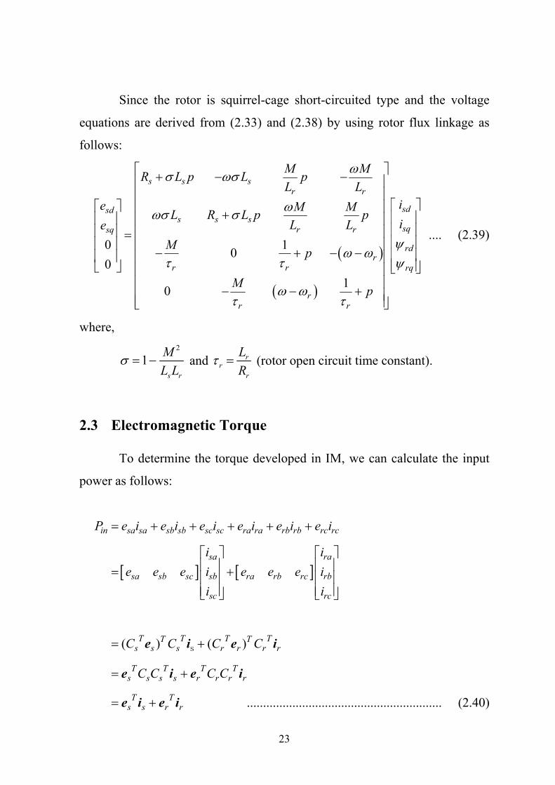
Since the rotor is squirrel-cage short-circuited type and the voltage

equations are derived from (2.33) and (2.38) by using rotor flux linkage as

follows:

0 100

10

s s sr r

sdsds s s

sqr rsq

rdr

r r rq

rr r

M MR L p L pL L

ie M ML R L p piL Le

M p

M p

.... (2.39)

where, 2

1s r

ML L

and rr

r

LR

(rotor open circuit time constant).

2.3 Electromagnetic Torque

To determine the torque developed in IM, we can calculate the input

power as follows:

in sa sa sb sb sc sc ra ra rb rb rc rcP e i e i e i e i e i e i

sa ra

sa sb sc sb ra rb rc rb

sc

in

rc

i ie e e i e e e i

i iP

( ) ( )T T T TT Ts s s r r r r

T T T Ts s s s r r r r

in C C C CP

C C C C

ｓe i e i

e i e i

T Ts s r rinP e i e i ............................................................ (2.40)

24

where,

1 112 2 23 3 30

2 2

sC

, 2 2cos cos cos2 22

3 2 2sin sin sin2 2

r r r

r

r r r

C

ss

s

ee

e , ss

s

ii

i , rr

r

ee

e , rr

r

ii

i

Therefore,

in s s s s r r r rP e i e i e i e i ............................... (2.41)

By using space vector, inP is expressed as

Rein s s r rP e i e i

Re s s s s s r r s r s

r r r r

in

r r r

i R i L pi M pi i M pi j M i

R i L

P

pi j L i

2 2 2 21 12 2s s r r s sin r rR i R i L p i L p iP

1 Re2 s r s r r s rM p i i i i j M i i ................. (2.42)

The each term of (2.42) is considered as 2

s sR i : primary copper loss

2r rR i : secondary copper loss

2 21 12 2s s r rL p i L p i : reactive power of self-inductance

25

1 ( )2 s r s rM p i i i i : reactive power of mutual inductance

Re( )r s rj M i i : mechanical power

Hence, the electromagnetic torque e is given by

*Re2

r s re

r

j M i i

P

*Im2 s reP M i i ........................................................... (2.43)

where, P : number of poles.

Therefore,

2e sq rd sd rqP M i i i i 2 sq rd d rq

re s

P M i iL

........... (2.44)

2.4 Non – linear State Equation

In order to compute the transient responses, we derive a non-linear

state equation from (2.39). The non-linear state equation is expressed as 2

r rqsd s rdsd sd sq

s s s r r s r r s r

Me R M Mpi i iL L L L L L L L

(2.45)

2sq rqs r rd

sq sd sqs s r r s r s r r s

e MR M Mpi i iL L L L L L L L

(2.46)

1rd sd rd r rq

r r

Mp i

....................................... (2.47)

1rq sq r rd rq

r r

Mp i

........................................ (2.48)

26

The mechanical equation of motion is expressed as

2

2 4 2r e L sq rd sd rq Lr

P M P Pp T i i TJ J L J

............... (2.49)

where, J : inertia of the rotor plus load, LT : load torque.

The above equations are described by a non-linear state equation

, ,s s s Lp Tx f x u ...................................................... (2.50)

where, sx is state vector and su is input vector of IM.

, , , ,T

s sd sq rd rq ri i x ............................. (2.51)

T

s sd sqe e u ..................................................... (2.52)

2.5 Linear State Equation

An essential problem connected to the modeling of the induction

machine is the non-linearity of the equations that describe its operation. This

non-linearity is caused by the voltage equations and the electromagnetic

torque relation as well, due to the products between the state variables. When

a control system is designed, it is very convenient to linearize the machine

equations [7], [8].

The stability analysis of non-linear system is difficult in general. So,

we derive a linear model of IM by considering small perturbation at a steady

state operating point which is obtained by setting 0p . The linear model of

IM is derived as follows from (2.50):

s s s s s L Lp T x A x B u B ................................... (2.53)

27

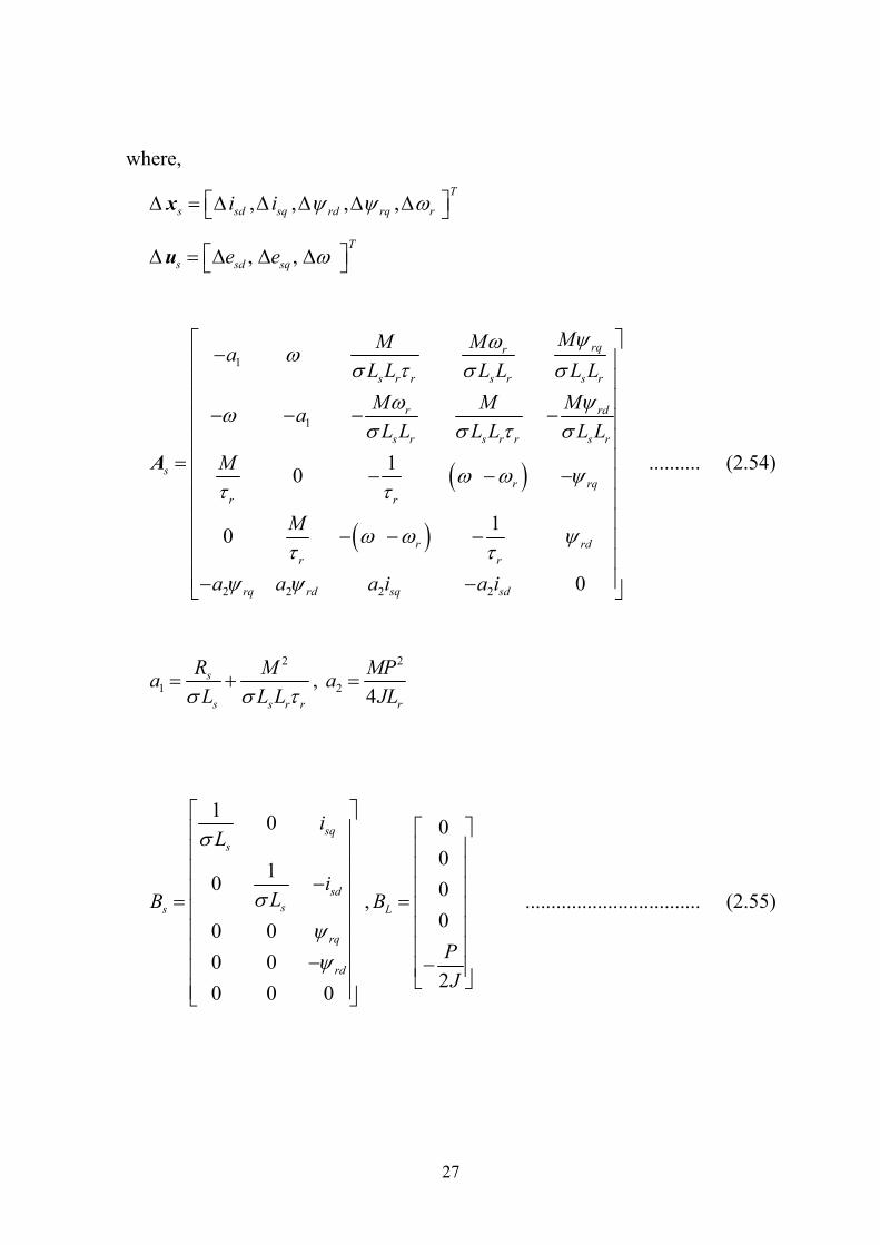
where,

, , , ,T

s sd sq rd rq ri i x

, ,T

s sd sqe e u

1

1

2 2 2 2

10

10

0

rqr

s r r s r s r

r rd

s r s r r s r

sr rq

r r

r rdr r

rq rd sq sd

MM MaL L L L L LM M MaL L L L L L

M

M

a a a i a i

A .......... (2.54)

2

1s

s s r r

R MaL L L

, 2

2 4 r

MPaJL

1 0

10

0 00 00 0 0

sqs

sdss

rq

rd

iL

iLB

,

0000

2

LB

PJ

.................................. (2.55)

28

Chapter 3

Speed Sensorless Vector Control

Systems

3.1 Proposed System A

A speed sensorless vector control system in which the rotor speed of

IM is estimated explicitly is proposed and analyzed to investigate the system

stability. We call the sensorless system “system A”.

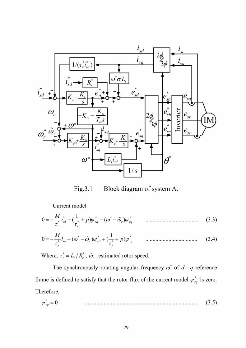
3.1.1 Block Diagram of System A

In order to simplify the controller and to stabilize the system at low

speed regenerating operations, the speed sensorless vector control system A is

proposed as shown in Fig.3.1. As described in (2.39), the d q rotating

reference frame equations of IM are modified as

Voltage model:

* * * * *( ) v vsd s s sd s sq rd rq

r r

M Me R L p i L i pL L

............... (3.1)

* * * * *( ) v vsq s sd s s sq rd rq

r r

M Me L i R L p i pL L

............... (3.2)

29

+*sdi

sdi

sae

sbe

sce

*sae*sbe

*sce

*sde

*sqe

*

sci

sai

+

+*r

1/ s

sqi

+

*s sdL i

+

* *1/( )r sdi

*sR

*sL

e

+*de+

23

23

*sdi

Inve

rter

+

+sqi

*sqi

ˆr

K

+pK iKs

pK + siK

+psK isKs

*

*

K

T s

Fig.3.1 Block diagram of system A.

Current model

* * * ** *

1 ˆ0 ( ) ( )sd rd r rqr r

M i p

.................................... (3.3)

* * ** *

1ˆ0 ( ) ( )sq r rd rqr r

M i p

.................................... (3.4)

Where, * *r r rL R , ˆr : estimated rotor speed.

The synchronously rotating angular frequency * of d q reference

frame is defined to satisfy that the rotor flux of the current model *rq is zero.

Therefore, * 0rq .............................................................................. (3.5)

30

This means that the d q axis is selected to synchronize the direction

of the current model rotor flux. By assuming that the d axis current

reference *sdi is constant, from (3.3) we have

* *rd sdMi ......................................................................... (3.6)

By substituting (3.5) and (3.6) into (3.4) we have

** *

ˆ sqr

r sd

ii

................................................................. (3.7)

Therefore, the estimated slip speed e is defined as

* *sq

er sd

ii

......................................................................... (3.8)

The assumption of constant *sdi causes that the d axis flux becomes

constant described in (3.6). Therefore, we make the following assumption:

0vrdp .......................................................................... (3.9)

By using (3.9), from (3.1) we have *

* * * * vsd s sd s sq rq

r

Me R i L iL

..................................... (3.10)

In (3.10), the induced voltage *de is defined as

** vd rq

r

MeL

............................................................... (3.11)

In the proposed system, the induced voltage *de is computed by using

the output voltage of d axis PI current controller. We can estimate the phase

of rotor flux * by changing * to satisfy

0vrq ............................................................................. (3.12)

31

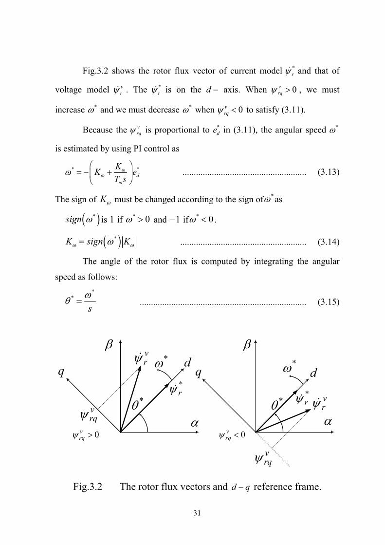
Fig.3.2 shows the rotor flux vector of current model *r and that of

voltage model vr . The *

r is on the d axis. When 0vrq , we must

increase * and we must decrease * when 0vrq to satisfy (3.11).

Because the vrq is proportional to *

de in (3.11), the angular speed *

is estimated by using PI control as

* *d

KK eT s

....................................................... (3.13)

The sign of K must be changed according to the sign of * as

*sign is 1 if * 0 and 1 if * 0 .

*K sign K ........................................................ (3.14)

The angle of the rotor flux is computed by integrating the angular

speed as follows: *

*

s .......................................................................... (3.15)

q

*

d*vr

vrq

q

*

d*

vr

vrq

0vrq 0v

rq

*r *

r

Fig.3.2 The rotor flux vectors and d q reference frame.

32

The rotor speed is estimated by using (3.7). The speed PI control and

q axis PI current control are composed like conventional system as shown

in Fig.3.1.

By assuming 0vrq and *v

rd sdM i , we have following equation

from (3.2): 2

* * * * * *( )sq s sd s s sq sdr

Me L i R L p i iL

* * ** ( )s s qs sd sq se L i R L p i .......................................... (3.16)

The 2 /3 transformation of Fig.3.1 is performed as

* * *

* * *

2 2cos cos cos3 32

3 2 2sin sin sin3 3

sasd

sbsq

sc

ii

ii

i

...... (3.17)

**

** * *

**

* *

cos sin2 2 2cos sin3 3 3

2 2cos sin3 3

sasd

sbsq

sc

ee

ee

e

...................... (3.18)

3.1.2 Description of System

The following assumptions are set in analysis.

(1) *sdi is constant.

(2) Voltage control is performed ideally and the following equation is

valid: *sa sae e , *

sb sbe e , *sc sce e ............................................ (3.19)

33

In order to analyze an IM, the d q reference frame that rotates

synchronously with the flux angle * is taken as of (2.26). Thus, * .

Therefore, the d q transformation is expressed as

* * *

* * *

2 2cos cos cos3 32

3 2 2sin sin sin3 3

sasd

sbsq

sc

ff

ff

f

. (3.20)

From (3.18), (3.19) and (3.20) we have *sd sde e , *

sq sqe e ........................................................... (3.21)

The PI d axis controller is expressed as

**d p sd sd cde K i i e ................................................... (3.22)

where,

*icd sd sd

Ke i is

............................................................ (3.23)

Then the derivative of cde is expressed as

*cd i sd sdpe K i i ......................................................... (3.24)

The PI angular speed estimator is expressed as * *

de K e ............................................................... (3.25)

where,

*d

Ke eT s

.................................................................... (3.26)

34

Then, the derivative of e is expressed as

*d

Kpe eT

................................................................. (3.27)

By using (3.22), we have

*p sd sd cd

Kpe K i i eT

....................................... (3.28)

From (3.22) and (3.25) * *

p sd p sd cde K K i K K i K e ............................... (3.29)

The output variable of PI speed controller *sqi is expressed as

* * ˆissq ps r r

Ki Ks

* **

**sq

ps r cdsqr sd

ii

i K

...................................... (3.30)

where,

* ** *sqis

cd rr sd

iKs i

............................................. (3.31)

By using * in (3.29), we have

* ** *sq

cd is r p sd p sd cdr sd

ip K K K i K K i K e e

i

....... (3.32)

The d axis voltage is expressed as

* * * * *sd p sd sd cd s sq s sde K i i e L i R i 　 ........................ (3.33)

The q – axis voltage is expressed as

* * * *isq p sq sq s sd

Ke K i i L is

* * **p sq sq cq s ssq dK i ee i L i .................................... (3.34)

35

where,

*icq sq sq

Ke i is

............................................................ (3.35)

Then, the derivative of cqe is expressed as

*cq i sq sqpe K i i ......................................................... (3.36)

3.1.3 Steady State Analysis

In this system, we can choose any value of speed command *r and

magnetizing current command *sdi . Load torque LT is an arbitrary input that

depends on any load connected to motor. When we set the *r , *

sdi , LT , other

all quantities can be determined. It has three degrees of freedom. In order to

simplify the procedure of computation, the slip speed is given instead of the

load torque.

Actually, angular frequency * , rotor speed r are constant in steady

state condition, and then the differential equation of the system becomes

linear. If the system is linear, it is similar to DC circuit. Then, we can set the

differential operator 0p in steady state analysis because there is no change

of state quantity.

The following equations is obtained by letting 0p in steady state

condition: *

sd sdi i , *sq sqi i , * 0de , 0cde , * ˆr r .............. (3.37)

36

From (2.39), the induction motor is expressed as *

* *sd s sd s sq rq

r

Me R i L iL

............................ (3.38)

** *

sq s sd s sq rdr

Me L i R iL

............................. (3.39)

*10 sd rd r rqr r

M i

............................ (3.40)

* 10 sq r rd rqr r

M i

............................ (3.41)

e LT ............................................................................ (3.42)

From (3.33) and (3.37), we have * * * *sd s sd s sqe R i L i .................................................. (3.43)

If we assume *s sR R , from (3.38) and (3.43), we have

0rq ............................................................................ (3.44)

From (3.40) and (3.44)

rd sdM i ..................................................................... (3.45)

From (3.41) and (3.44),

**

sq sqr

r rd r sd

M i ii

............................................... (3.46)

37

By assuming *r rR R and using (3.7), we have

ˆr r ........................................................................... (3.47)

Therefore, *

r r ........................................................................... (3.48)

By comparing (3.34) and (3.39), we have

cq s sqe R i ....................................................................... (3.49)

A steady-state solution is calculated in the following procedures by

setting * 1minrN , 1minslN , and *sdi as given values.

[1] Electrical angular speed command *r is calculated by

** 2

2 60r

rP N .................................................................. (3.50)

[2] Similarly, electrical slip angular frequency sl is calculated by

* 22 60

slsl r

P N ................................................. (3.51)

[3] 0rq is calculated by referred to(3.12)

[4] rd sdM i

[5] sqi is calculated by

sl rsq rdi

M ................................................................. (3.52)

38

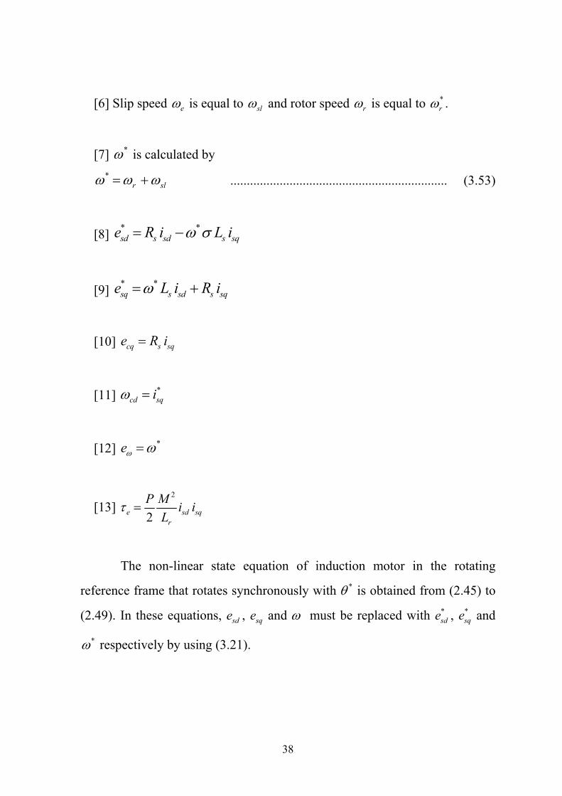
[6] Slip speed e is equal to sl and rotor speed r is equal to *r .

[7] * is calculated by *

r sl .................................................................. (3.53)

[8] * *sd s sd s sqe R i L i

[9] * *sq s sd s sqe L i R i

[10] cq s sqe R i

[11] *cd sqi

[12] *e

[13] 2

2e sd sqr

P M i iL

The non-linear state equation of induction motor in the rotating

reference frame that rotates synchronously with * is obtained from (2.45) to

(2.49). In these equations, sde , sqe and must be replaced with *sde , *

sqe and

* respectively by using (3.21).

39

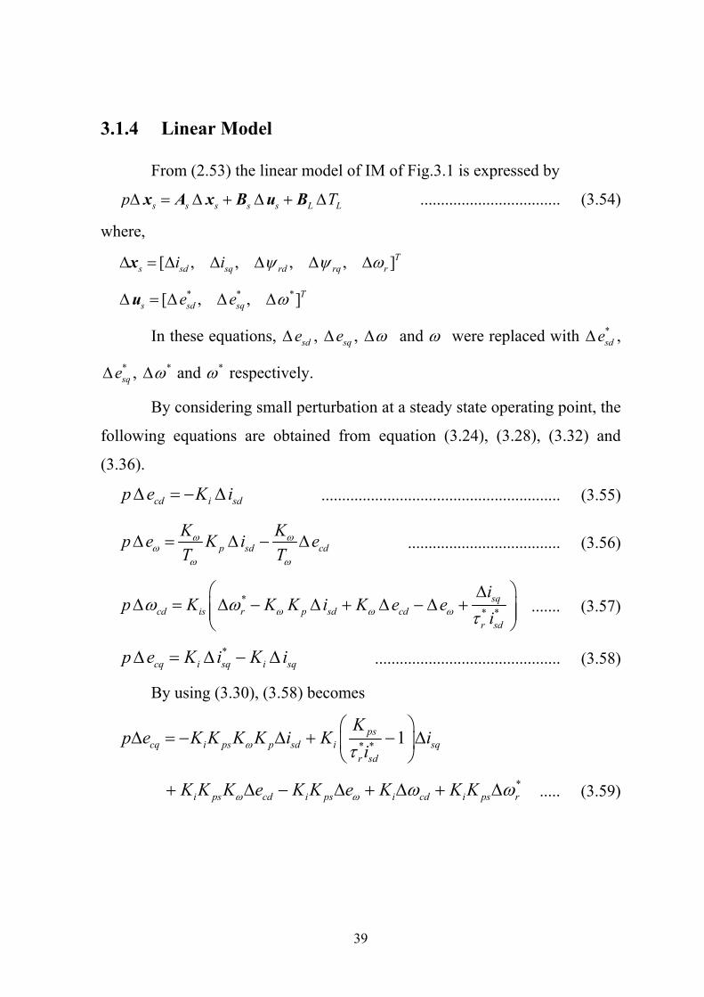
3.1.4 Linear Model

From (2.53) the linear model of IM of Fig.3.1 is expressed by

s s s s s L Lp T x A x B u B .................................. (3.54)

where,

[ , , , , ]Ts sd sq rd rq ri i x

* * *[ , , ]Ts sd sqe e u

In these equations, sde , sqe , and were replaced with *sde ,

*sqe , * and * respectively.

By considering small perturbation at a steady state operating point, the

following equations are obtained from equation (3.24), (3.28), (3.32) and

(3.36).

cd i sdp e K i .......................................................... (3.55)

p sd cdK Kp e K i eT T

..................................... (3.56)

** *

sqcd is r p sd cd

r sd

ip K K K i K e e

i

....... (3.57)

*cq i sq i sqp e K i K i ............................................. (3.58)

By using (3.30), (3.58) becomes

* * 1pscq i ps p sd i sq

r sd

Kp e K K K K i K i

i

*i ps cd i ps i cd i ps rK K K e K K e K K K ..... (3.59)

40

These equations can be expressed in a matrix form as follows:

* *

* *

0 0 0 0

0 0 0 0

0 0 0

1 0 0 0

0 0 0 0

0 0 0

0 0

i

sdpcdsq

is rdpiscd r sd rqcq

ps rps pi i

r sd

is is

psi i

KK iKe T i

e Kp K K Ki

eK

K K K K Ki

KT

K K KK K K K K

*

00

0

cd

riscd

cq psips i

ee

Ke K KK

Simply is expressed as

x z rp z = A x + A z + B r ....................................... (3.60)

where, T

cd cd cqe e e z = , *r r =

From the equations (3.29), (3.33) and (3.34) we have *

p sd cdK K i K e e ..................................... (3.61)

* * *sd p sd cd s sq s sqe K i e L i L i

* *1p s sq sd s ssd qK K L i ie L i

* 1s sq cd sd qs sK L i e L i ee .......................... (3.62)

41

* * * *sq p sq p sq cq s sde K i K i e L i

** *

* 1psp ps r p cd p sq

r sdsq

KK K K K ie

i

* *cq s sd p ps p sdsq e L i K K K ie K

* * *p ps s sd cd s sd p pssq K K L i K e L i K K ee ........... (3.63)

We can write a matrix form of su as follows:

x s zF F F s ru x z + r .......................................... (3.64)

*

*

* ** *

*

* *

1 0 0 0

1 0 0 0

0 0 0 0

1 0 0

1

1 0 0

sdp s sq s

sd sqps

sq p s sd p ps p rdr sd

rqp

r

s sq s sq

p ps s sd s sd p ps p

iK K L i Le i

Ke K K L i K K K

iK K

K L i L i

K K K L i L i K K K

K

*

0

0

cd

p ps rcd

cq

ee

K K

e

From equation (3.54), (3.61) and (3.64) the linear model of proposed

system A can be derived as follows:

0

s s x s z s rs s LL

x z r

p T

A B F B F B Fx x Br

A A Bz z .... (3.65)

Simply we can express as

s L Lp T x A x B r + B ....................................... (3.66)

42

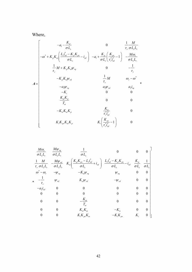
Where,

1

**

1 * *

*

2 2 2

* *

* *

10

1

1 10

1

0 0

0 0

0

1

p

s r s r

s sd p ps p ps rp sd

s s r sd s r

p rqr r

p rd rr

rq rd sq

i

p

isis p

r sd

psi ps p i

r sd

K MaL L L

L i K K K K MK K i aL L i L L

M K K

K K M

a a a iK

K KT

KK K Ki

KK K K K K

i

A *

0

* *

*

2

1 0 0 0

1 1

0 01 0 0*

0 0 0 0 00 0 0 0 0 0

0 0 0 0 0

0 0 0 00 0 0

rqr

s r s r s

p ps s sd s sd p ps prdsd sd

r s r s r s s s s

r rq rq rq

rd rd rdr

sd

is is

i ps i ps i

MML L L L L

K K L i L i K K KM M K i iL L L L L L L L

K

K

a i

KT

K K KK K K K K K

43

0 0

0

0 00 0

02

0 00 0

00

p ps

s

is

i ps

K KL

PJ

KK K

B,

0000

20000

LPJ

B

The output equation is expressed as

y C x ...................................................................... (3.67)

Where,

0 0 0 0 1 0 0 0 0C

44

3.2 Proposed System B

In the proposed system B, q axis current controller is removed.

Therefore, the system B is simpler than the system A.

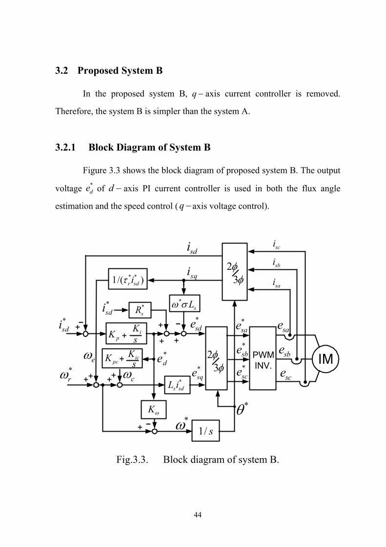
3.2.1 Block Diagram of System B

Figure 3.3 shows the block diagram of proposed system B. The output

voltage *de of d axis PI current controller is used in both the flux angle

estimation and the speed control ( q axis voltage control).

IM

+*sdi

sdi

*

sae

sbe

sce

*sae*sbe*sce

*sde

*sqe

*

sci

sbi

sai

++*r

1/ s

sqi

+

*s sdL i++

+

PWMINV.

* *1/( )r sdi

*sR

*sL

e

+

c

*de

+

23

23

*sdi

pK iK+ s

+pcK icKs

K

Fig.3.3. Block diagram of system B.

45

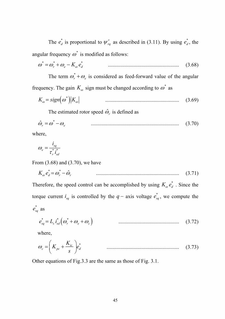
The *de is proportional to v

rq as described in (3.11). By using *de , the

angular frequency * is modified as follows: * * *

r e dK e ...................................................... (3.68)

The term *r e is considered as feed-forward value of the angular

frequency. The gain K sign must be changed according to * as

*K sign K ........................................................ (3.69)

The estimated rotor speed ˆr is defined as

*ˆr e ................................................................... (3.70)

where,

* *sq

er sd

ii

From (3.68) and (3.70), we have * * ˆd r rK e ............................................................... (3.71)

Therefore, the speed control can be accomplished by using *dK e . Since the

torque current sqi is controlled by the q axis voltage *sqe , we compute the

*sqe as

* * *sq s sd r e ce L i .............................................. (3.72)

where,

*icc pc d

KK es

....................................................... (3.73)

Other equations of Fig.3.3 are the same as those of Fig. 3.1.

46

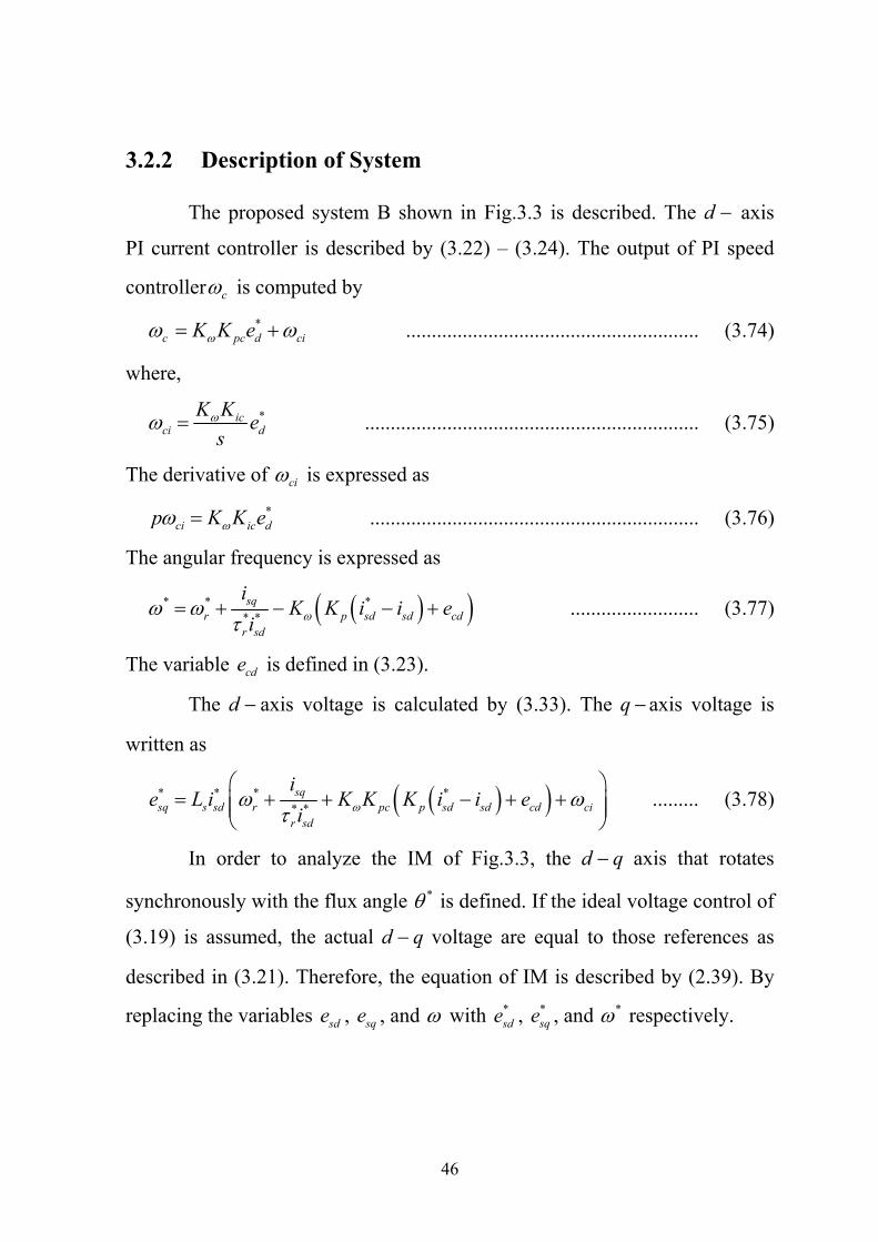
3.2.2 Description of System

The proposed system B shown in Fig.3.3 is described. The d axis

PI current controller is described by (3.22) – (3.24). The output of PI speed

controller c is computed by *

c pc d ciK K e ......................................................... (3.74)

where,

*icci d

K K es ................................................................. (3.75)

The derivative of ci is expressed as *

ci ic dp K K e ................................................................ (3.76)

The angular frequency is expressed as

* * ** *sq

r p sd sd cdr sd

iK K i i e

i

......................... (3.77)

The variable cde is defined in (3.23).

The d axis voltage is calculated by (3.33). The q axis voltage is

written as

* * * ** *sq

sq s sd r pc p sd sd cd cir sd

ie L i K K K i i e

i

......... (3.78)

In order to analyze the IM of Fig.3.3, the d q axis that rotates

synchronously with the flux angle * is defined. If the ideal voltage control of

(3.19) is assumed, the actual d q voltage are equal to those references as

described in (3.21). Therefore, the equation of IM is described by (2.39). By

replacing the variables sde , sqe , and with *sde , *

sqe , and * respectively.

47

3.2.3 Steady State Analysis

At steady state condition, the derivative operator p is set to zero. By

the integral controllers of d axis current and speed, we have *

sd sdi i ............................................................................. (3.79) * 0de ............................................................................... (3.80)

Therefore, 0cde from (3.22).

The actual IM equations at steady state are described in (3.38) – (3.42).

By assuming *s sR R , the q axis flux rq becomes zero as the same of

system A. Therefore, (3.46) is valid in this case too. From (3.80), we have

* ** *sq

rr sd

ii

................................................................ (3.81)

By assuming *r rR R , the following equation is obtained from (3.46)

and (3.81): *r r

From (3.78) and (3.81), we have * * * *sq s sd ci s sde L i L i .................................................... (3.82)

By comparing (3.39), (3.45) and (3.82)

*s sq

cis sd

R iL i

...................................................................... (3.83)

Steady-state values are calculated by giving *rN , slN and *

sdi as known

values, similar to the case of system A.

48

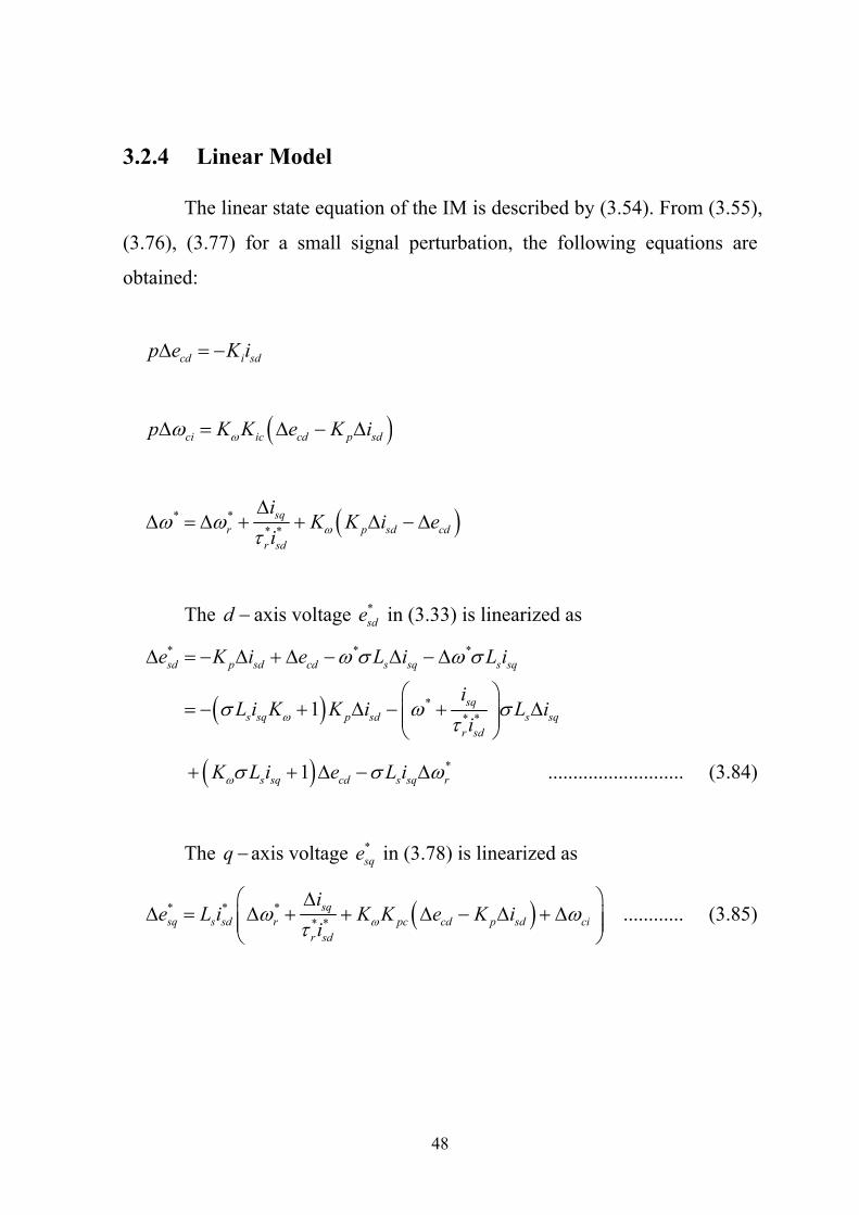
3.2.4 Linear Model

The linear state equation of the IM is described by (3.54). From (3.55),

(3.76), (3.77) for a small signal perturbation, the following equations are

obtained:

cd i sdp e K i

ci ic cd p sdp K K e K i

* ** *

sqr p sd cd

r sd

iK K i e

i

The d axis voltage *sde in (3.33) is linearized as

*

* * *

** *1

sd p sd cd s sq s sq

sqs sq p sdsd s sq

r sd

e K i e L i L i

iL i K K i L i

ie

*1s sq cd s sq rK L i e L i ........................... (3.84)

The q axis voltage *sqe in (3.78) is linearized as

* * ** *

sqsq s sd r pc cd p sd ci

r sd

ie L i K K e K i

i

............ (3.85)

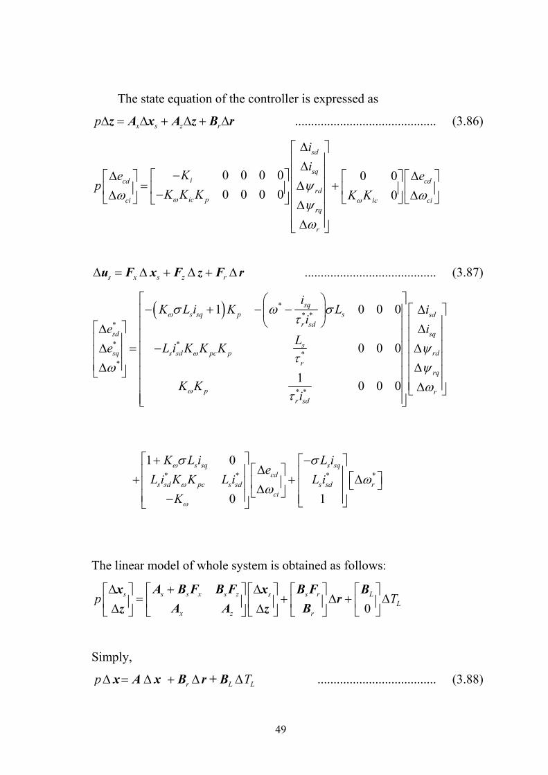
49

The state equation of the controller is expressed as

x s z rp z A x A z B r ............................................ (3.86)

0 0 0 0 0 00 0 0 0 0

sd

sqicd cd

rdic pci ic ci

rq

r

ii

Ke ep

K K K K K

s x s z r u F x F z F r ......................................... (3.87)

** *

*

* **

*

* *

* *

1 0 0 0

0 0 0

1 0 0 0

1 0

0

sqs sq p s sd

r sdsd sq

ssq s sd pc p rd

rrq

p rr sd

s sq

s sd pc s sd

iK L i K L i

ie i

Le L i K K K

K Ki

K L ie

L i K K L iK

* *

1

s sqcd

s sd rci

L iL i

The linear model of whole system is obtained as follows:

0s s x s z s rs s L

Lx z r

p T

A B F B F B Fx x Br

A A Bz z

Simply,

r L Lp T x A x B r + B ..................................... (3.88)

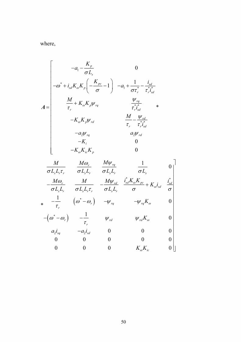
50

where,

1

*1 * * *

* *

* *

2 2

0

11

*

00

p

s

pc sdsd p

r r sd

rqp rq

r r sd

rdp rd

r r sd

rq rd

i

ic p

Ka

LK ii K K a

i

M K Ki

MK Ki

a aK

K K K

A

* *

*

*

2 2

1 0

1 0*

1 0

0 0 00 0 0 0 00 0 0 0

rqr

s r r s r s r s

sd pcr rd sdsd

s r s r r s r

r rq rqr

r rd rdr

sq sd

ic

MM ML L L L L L L

i K KM M M iK iL L L L L L

K

K

a i a i

K K

51

*

0

000

sdsd

rq

rd

i i

B ,

0000

200

LPJ

B

The output equation is expressed as

y C x ........................................................................ (3.89)

where,

0 0 0 0 1 0 0C

3.3 Gain Selection of Controller

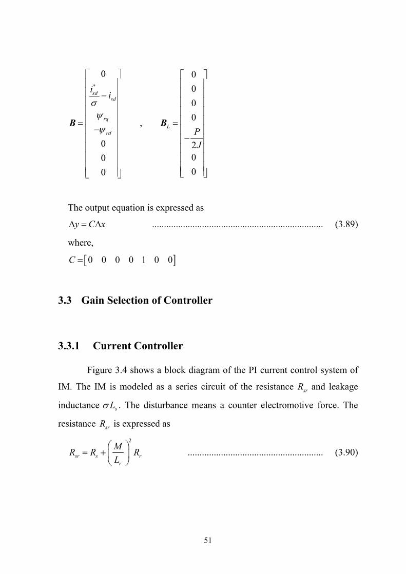
3.3.1 Current Controller

Figure 3.4 shows a block diagram of the PI current control system of

IM. The IM is modeled as a series circuit of the resistance srR and leakage

inductance sL . The disturbance means a counter electromotive force. The

resistance srR is expressed as 2

sr s rr

MR R RL

......................................................... (3.90)

52

*( )I s ( )I s1sr sR L s

11pi

KT s

Fig.3.4 Block diagram of the current control system.

Assuming that there are no disturbances, the closed-loop transfer

function of the current control becomes the following equations:

*

11

p i

s sr i p i

K T sII L s R T s K T s

The iT is usually designed as [45]

si

sr

LTR

.......................................................................... (3.91)

The current transfer function becomes as

*1

1p

s p eq

KII L s K T s

............................................... (3.92)

where,

seq

p

LTK

Cut-off frequency c of this transfer function is expressed by the

following equation:

1pc

sr i eq

KR T T

............................................................... (3.93)

53

By setting the cut-off frequency c , the proportional gain pK is

determined by (3.93).

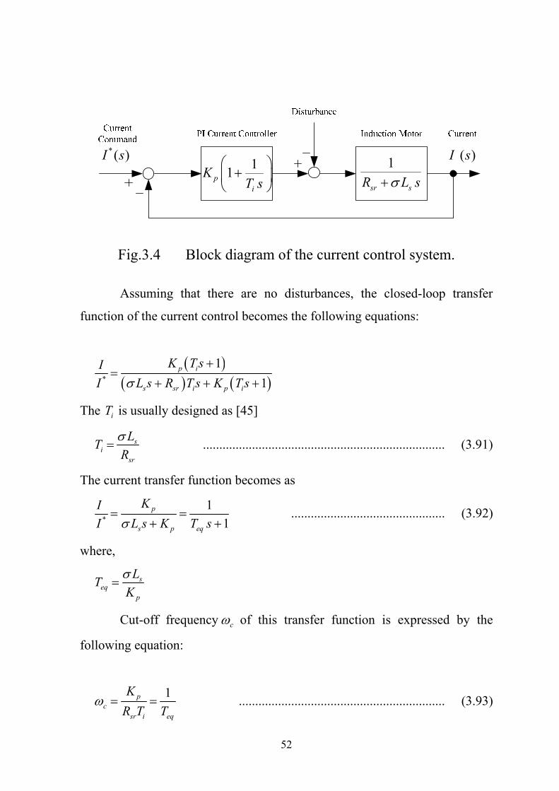
3.3.2 Speed Controller

The block diagram of speed control system is shown in Fig.3.5. When

the vector control is ideal, the torque can be controlled as

2

*

2e sd sq T sqr

PM i i K iL

..................................................... (3.94)

The loop transfer function 0G of Fig. 3.5 is

01

1 2is T

pseq

K PKG Ks T s Js

........................................ (3.95)

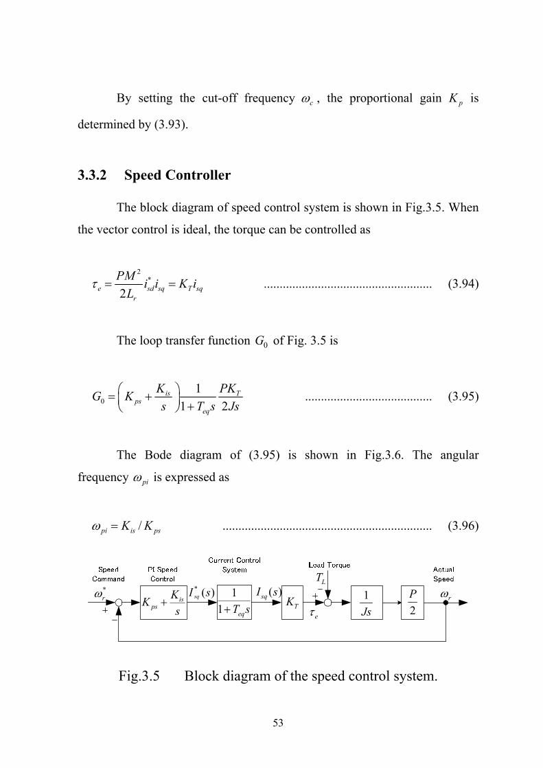
The Bode diagram of (3.95) is shown in Fig.3.6. The angular

frequency pi is expressed as

/pi is psK K .................................................................. (3.96)

* ( )sqI s ( )sqI sis

psKKs

1

1 eqT s TK 1Js

LT

e

*r

2P r

Fig.3.5 Block diagram of the speed control system.

54

pi

2TPK

Js

csc

-40 dB/dec isps

KKs

11 eqT s

0 dB

-20 dB/dec

-20 dB/dec

Gai

n

Fig.3.6 Bode diagram of loop transfer function 0G .

In order to have sufficient phase margin, the following equation

should be satisfied [45]:

/5pi sc ...................................................................... (3.97)

Under the condition (3.97), the crossover frequency sc is obtained as

2T ps

sc

PK KJ

.................................................................. (3.98)

If we set the pi and sc , the gains psK and isK is determined by (3.98) and

(3.96).

55

Chapter 4

Simulation and Experimental

Results

4.1 Experimental System

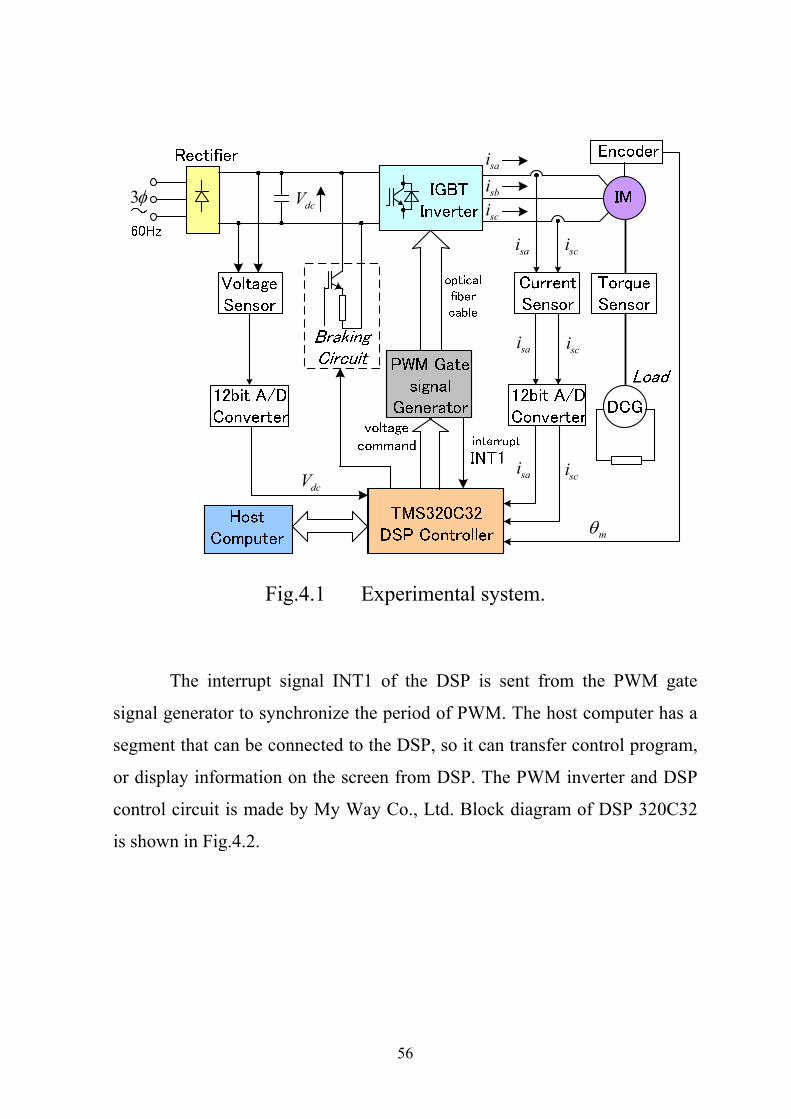
4.1.1 Microcomputer control system

The IM control system by using a digital signal processor (DSP) is

shown in Fig.4.1. The power circuit is composed by rectifier, smoothing

capacitor, and IGBT inverter. A DC machine is used as a load through a

torque sensor for the induction machine. Torque sensor is used for detecting

the torsion of the shaft. The motor currents and DC link voltage are detected

to the DSP through an analog to digital (A/D) converter.

PWM gate signal generator is connected to IGBT inverter. These

signals are carried by an optical fiber cable and are not affected by noise.

Resistor is connected to the braking circuit and the regenerative energy is

consumed as heat. When the IM operates as a generator, IGBT brake circuit is

turned on. The dangerous voltage rise can damage the rectifier circuit diode

and the smoothing capacitor, because its energy is not returned to the power

supply.

56

3

dcV

sai

sbisci

sai

sai

sai

sci

sci

sci

m

dcV

Fig.4.1 Experimental system.

The interrupt signal INT1 of the DSP is sent from the PWM gate

signal generator to synchronize the period of PWM. The host computer has a

segment that can be connected to the DSP, so it can transfer control program,

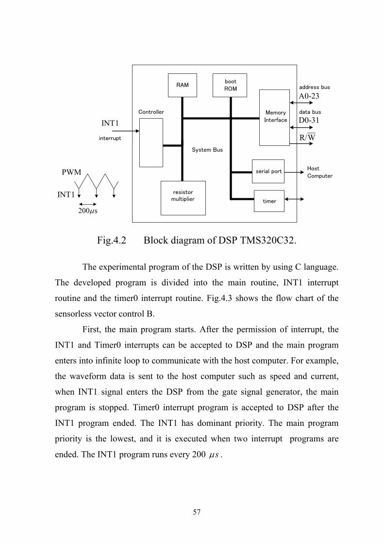
or display information on the screen from DSP. The PWM inverter and DSP

control circuit is made by My Way Co., Ltd. Block diagram of DSP 320C32

is shown in Fig.4.2.

57

bootROM

RAM

INT1

A0-23

D0-31

R/Winterrupt

Controller

System Bus

timer

serial port

address bus

data busMemory Interface

resistormultiplier

HostComputer

INT1

PWM

200 s Fig.4.2 Block diagram of DSP TMS320C32.

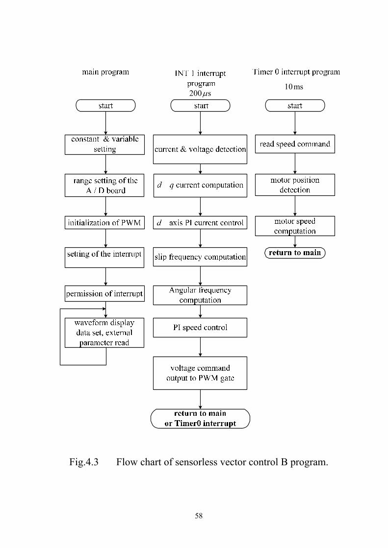
The experimental program of the DSP is written by using C language.

The developed program is divided into the main routine, INT1 interrupt

routine and the timer0 interrupt routine. Fig.4.3 shows the flow chart of the

sensorless vector control B.

First, the main program starts. After the permission of interrupt, the

INT1 and Timer0 interrupts can be accepted to DSP and the main program

enters into infinite loop to communicate with the host computer. For example,

the waveform data is sent to the host computer such as speed and current,

when INT1 signal enters the DSP from the gate signal generator, the main

program is stopped. Timer0 interrupt program is accepted to DSP after the

INT1 program ended. The INT1 has dominant priority. The main program

priority is the lowest, and it is executed when two interrupt programs are

ended. The INT1 program runs every 200 s .

58

200 s10ms

Fig.4.3 Flow chart of sensorless vector control B program.

59

The experimental programs are changed to machine language by using

C compiler and sent to RAM of DSP. This process is called “downloading”.

Process and communication program commands are made by My Way Co.

Ltd. It is necessary for both the DSP and the PC.

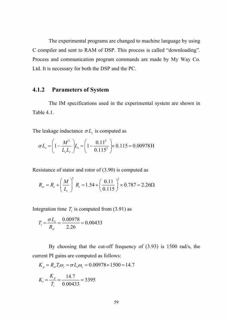
4.1.2 Parameters of System

The IM specifications used in the experimental system are shown in

Table 4.1.

The leakage inductance sL is computed as

2 2

20.111 1 0.115 0.00978H

0.115s ss r

ML LL L

Resistance of stator and rotor of (3.90) is computed as 2 20.111.54 0.787 2.26

0.115sr s rr

MR R RL

Integration time iT is computed from (3.91) as

0.00978 0.004332.26

si

sr

LTR

By choosing that the cut-off frequency of (3.93) is 1500 rad/s, the

current PI gains are computed as follows:

0.00978 1500 14.7p sr i c s cK R T L

14.7 33950.00433

pi

i

KK

T

60

Table 4.1 Parameters of the three-phase IM.

Number of poles P[poles] 4

Rated Output [kW] 1.5

Rated Torque [N-m] 8.43

Speed [min-1] 1700

Rated Line Voltage [V] 200

Rated Current [A] 6.4

Excitation Current *sdi [A] 4.2

Moment Inertia J[kg・m2] 0.0126

Primary Resistance Nominal Value Rs[Ω] 1.54

Secondary Resistance Nominal Value Rr[Ω] 0.787

Iron Loss Resistance Rm[Ω] 391

Primary Self-inductance Ls[H] 0.115

Secondary Self-Inductance Lr[H] 0.115

Mutual Inductance M[H] 0.11

Motor Manufacturer Mitsubishi Electric

Corporation

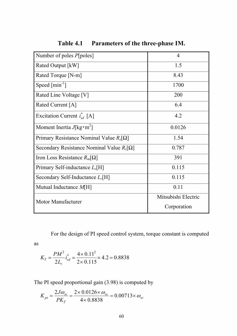
For the design of PI speed control system, torque constant is computed

as 2 2

* 4 0.11 4.2 0.88382 2 0.115T sd

r

PMK iL

The PI speed proportional gain (3.98) is computed by

2 2 0.0126 0.007134 0.8838

sc scps sc

T

JKPK

61

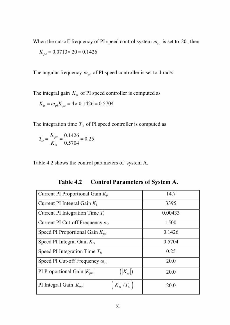
When the cut-off frequency of PI speed control system sc is set to 20 , then

0.0713 20 0.1426psK

The angular frequency pi of PI speed controller is set to 4 rad/s.

The integral gain isK of PI speed controller is computed as

4 0.1426 0.5704is pi psK K

The integration time isT of PI speed controller is computed as

0.1426 0.250.5704

psis

is

KT

K

Table 4.2 shows the control parameters of system A.

Table 4.2 Control Parameters of System A.

Current PI Proportional Gain Kp 14.7

Current PI Integral Gain Ki 3395

Current PI Integration Time Ti 0.00433

Current PI Cut-off Frequency ωc 1500

Speed PI Proportional Gain Kps 0.1426

Speed PI Integral Gain Kis 0.5704

Speed PI Integration Time Tis 0.25

Speed PI Cut-off Frequency ωsc 20.0

PI Proportional Gain |Kpω| K 20.0

PI Integral Gain |Kiω| /K T 20.0

62

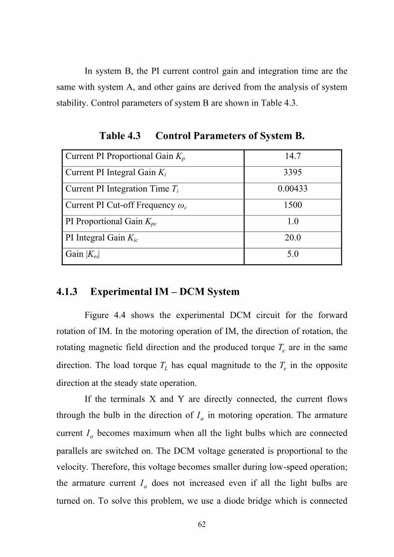
In system B, the PI current control gain and integration time are the

same with system A, and other gains are derived from the analysis of system

stability. Control parameters of system B are shown in Table 4.3.

Table 4.3 Control Parameters of System B.

Current PI Proportional Gain Kp 14.7

Current PI Integral Gain Ki 3395

Current PI Integration Time Ti 0.00433

Current PI Cut-off Frequency ωc 1500

PI Proportional Gain Kpc 1.0

PI Integral Gain Kic 20.0

Gain |Kω| 5.0

4.1.3 Experimental IM – DCM System

Figure 4.4 shows the experimental DCM circuit for the forward

rotation of IM. In the motoring operation of IM, the direction of rotation, the

rotating magnetic field direction and the produced torque eT are in the same

direction. The load torque LT has equal magnitude to the eT in the opposite

direction at the steady state operation.

If the terminals X and Y are directly connected, the current flows

through the bulb in the direction of aI in motoring operation. The armature

current aI becomes maximum when all the light bulbs which are connected

parallels are switched on. The DCM voltage generated is proportional to the

velocity. Therefore, this voltage becomes smaller during low-speed operation;

the armature current aI does not increased even if all the light bulbs are

turned on. To solve this problem, we use a diode bridge which is connected

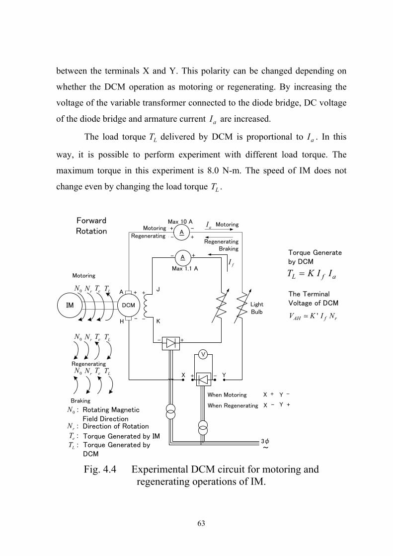
63

between the terminals X and Y. This polarity can be changed depending on

whether the DCM operation as motoring or regenerating. By increasing the

voltage of the variable transformer connected to the diode bridge, DC voltage

of the diode bridge and armature current aI are increased.

The load torque LT delivered by DCM is proportional to aI . In this

way, it is possible to perform experiment with different load torque. The

maximum torque in this experiment is 8.0 N-m. The speed of IM does not

change even by changing the load torque LT .

DCM

A

H

+

-

A

A

+

-

J

K

3φ～

When Motoring

When Regenerating

+-

+ -

- +

Motoring ：

Regenerating ：

Motoring

Regenerating

Max 10 A

Max 1.1 A

Ｖ

+ -

+-

Forward Rotation

IM Light Bulb

X Y

X

X

Y

Y

+

+

-

-

Motoring

Regenerating

Direction of Rotation

Torque Generated by IM Torque Generated by

DCM

L f aT K I I

'AH f rV K I N

Torque Generate by DCM

The Terminal Voltage of DCM

Braking

Rotating Magnetic Field Direction

Braking

0N rN eT LT

0N rN eT LT

0N rN eT LT

0 :N

:rN:eT:LT

aI

fI

Fig. 4.4 Experimental DCM circuit for motoring and

regenerating operations of IM.

64

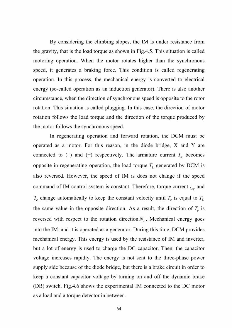
By considering the climbing slopes, the IM is under resistance from

the gravity, that is the load torque as shown in Fig.4.5. This situation is called

motoring operation. When the motor rotates higher than the synchronous

speed, it generates a braking force. This condition is called regenerating

operation. In this process, the mechanical energy is converted to electrical

energy (so-called operation as an induction generator). There is also another

circumstance, when the direction of synchronous speed is opposite to the rotor

rotation. This situation is called plugging. In this case, the direction of motor

rotation follows the load torque and the direction of the torque produced by

the motor follows the synchronous speed.

In regenerating operation and forward rotation, the DCM must be

operated as a motor. For this reason, in the diode bridge, X and Y are

connected to (–) and (+) respectively. The armature current aI becomes

opposite in regenerating operation, the load torque LT generated by DCM is

also reversed. However, the speed of IM is does not change if the speed

command of IM control system is constant. Therefore, torque current sqi and

eT change automatically to keep the constant velocity until eT is equal to LT

the same value in the opposite direction. As a result, the direction of eT is

reversed with respect to the rotation direction rN . Mechanical energy goes

into the IM; and it is operated as a generator. During this time, DCM provides

mechanical energy. This energy is used by the resistance of IM and inverter,

but a lot of energy is used to charge the DC capacitor. Then, the capacitor

voltage increases rapidly. The energy is not sent to the three-phase power

supply side because of the diode bridge, but there is a brake circuit in order to

keep a constant capacitor voltage by turning on and off the dynamic brake

(DB) switch. Fig.4.6 shows the experimental IM connected to the DC motor

as a load and a torque detector in between.

65

0N

I

II

III

rN

eTLT

0N

0N

rN

rN

eT

eT

LT

LT

0N

rNeT

LT eT

N0N N

( 0)s 0N

( 1)s

III III

lT

LT

I

Motoring operationPlugging Regenerating operation Fig.4.5 Operating regions of IM.

Fig.4.6 IM with DCM as a load and a torque detector in between.

66

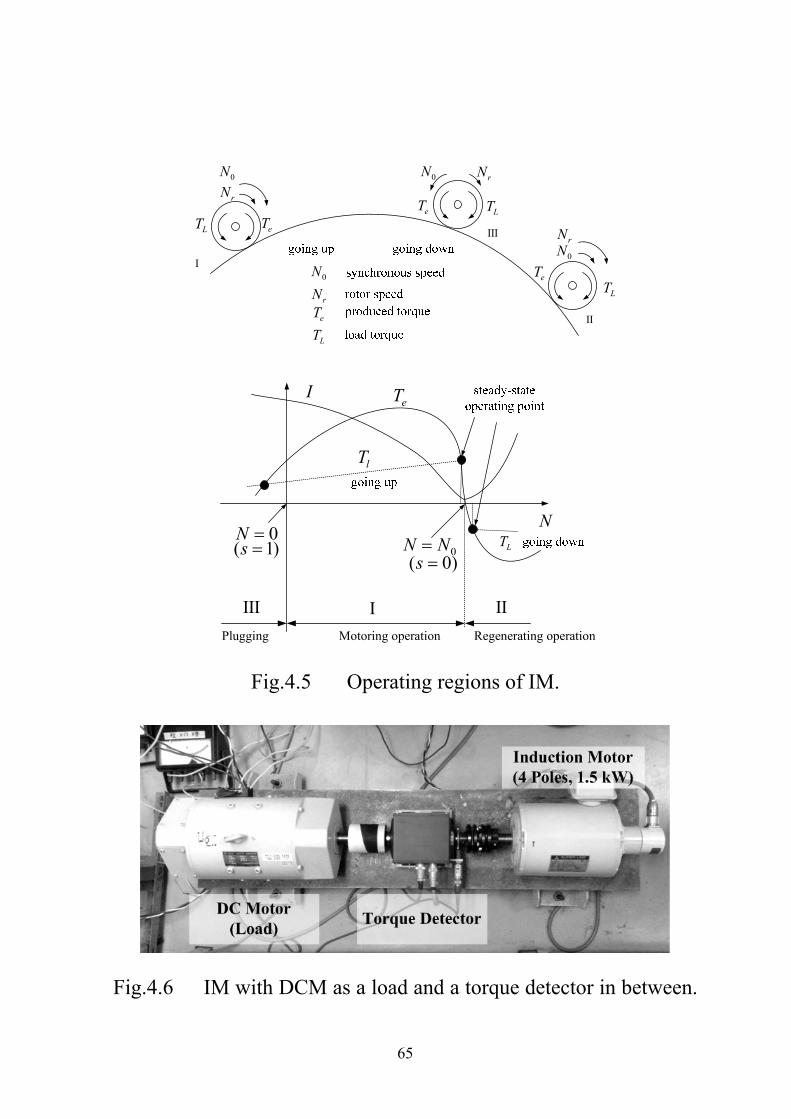
4.2 System Stability

Figure 4.7 shows the root trajectories that are computed by the linear

model of proposed system B. The speed command *rN is 1700 min , and slip

speed slN are changed from 180min to 180min as parameter of load. The

different integral gain icK such as 100.0, 50.0, 33.3, 25.0 and 20.0 are

selected. If the integral gain icK is very large, the system becomes unstable.

However, if icK is selected smaller than 100.0, the system is stable at both

motoring and regenerating operation.

: 100.0icK

: 50.0: 33.3: 25.0: 20.0

* -1700 min3.0

rNK

1

10

10

1 5

10

5

1

1010

1

122

3

4

53

6789

-1minslN 1 : -80

10 : 809 : 608 : 357 : 206 : 55 : 04 : -203 : -352 : -60

Fig.4.7 Root trajectories with parameters of slip speed slN and

integral gain icK (system B).

67

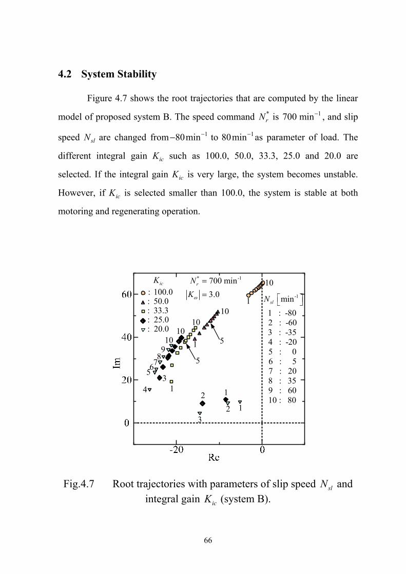
Figure 4.8 shows the root trajectories when the gain K and the

integral gain icK are changed. The speed command *rN is 1700min , and slip

speed slN is 135.0min . It is observed that the system becomes stable by

choosing larger value of K and smaller value of icK .

* -1

1700 min35 min

r

sl

NN

1 : 0.01

2 : 0.13 : 0.54 : 1.05 : 1.56 : 2.07 : 3.08 : 5.09 : 1010 : 100

K

: 100.0: 50.0: 33.3: 20.0: 10.0

icK1

2

34

44

4

4

5

55

5

5

6

6

6

6

6

7

7

7

7

7

8

8

8

8

8

9

9

9

9

9

10

10

10

10

10

Fig.4.8 Root trajectories with parameters of integral gain icK

and gain K (system B).

68

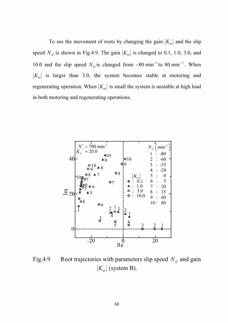
To see the movement of roots by changing the gain K and the slip

speed slN is shown in Fig.4.9. The gain K is changed to 0.1, 1.0, 3.0, and

10.0 and the slip speed slN is changed from 180 min to 180 min . When

K is larger than 3.0, the system becomes stable at motoring and

regenerating operation. When K is small the system is unstable at high load

in both motoring and regenerating operations.

: 0.1: 1.0: 3.0: 10.0

K

* -1700 min20.0

r

ic

NK

1

111

10

2

22

3

3

34

4

4

5

55

6

66 7

77

88

8

99

9

1010

10

-1minslN 1 : -80

10 : 809 : 608 : 357 : 206 : 55 : 04 : -203 : -352 : -60

Fig.4.9 Root trajectories with parameters slip speed slN and gain

K (system B).

69

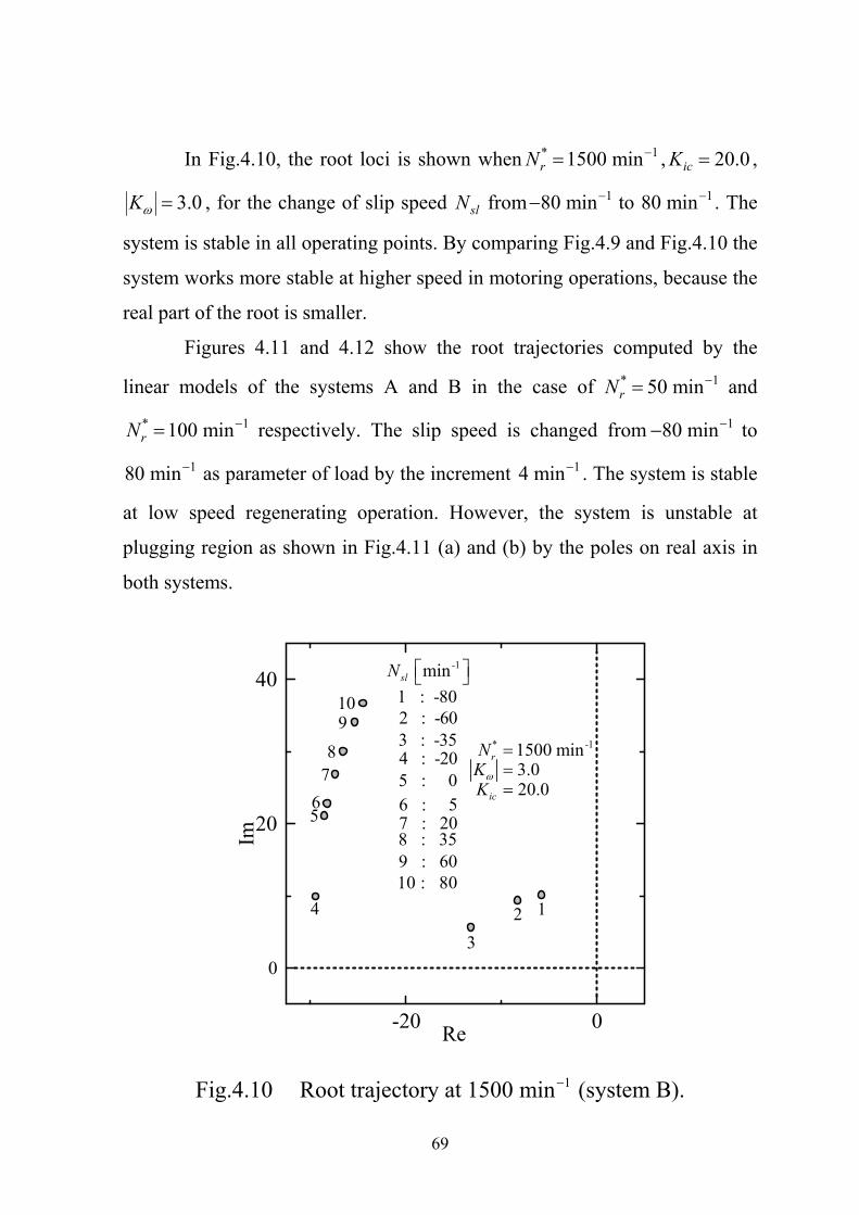
In Fig.4.10, the root loci is shown when * 11500 minrN , 20.0icK ,

3.0K , for the change of slip speed slN from 180 min to 180 min . The

system is stable in all operating points. By comparing Fig.4.9 and Fig.4.10 the

system works more stable at higher speed in motoring operations, because the

real part of the root is smaller.

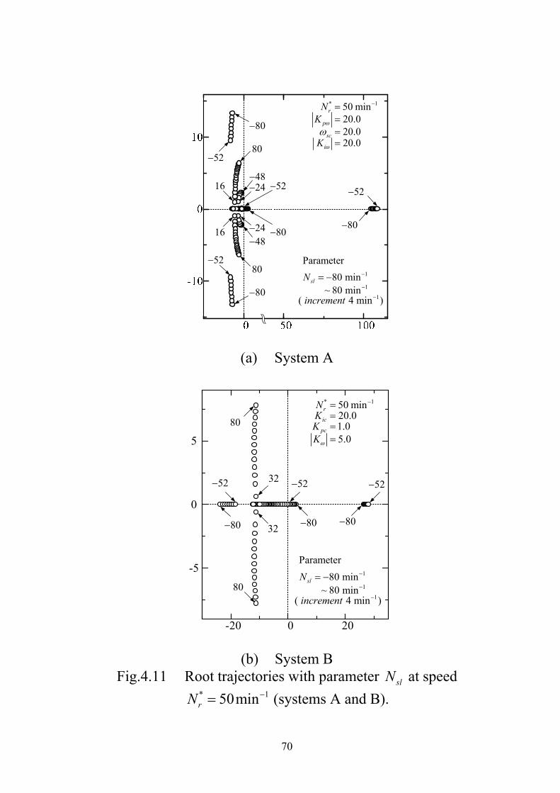
Figures 4.11 and 4.12 show the root trajectories computed by the

linear models of the systems A and B in the case of * 150 minrN and

* 1100 minrN respectively. The slip speed is changed from 180 min to

180 min as parameter of load by the increment 14 min . The system is stable

at low speed regenerating operation. However, the system is unstable at

plugging region as shown in Fig.4.11 (a) and (b) by the poles on real axis in

both systems.

-1minslN 1 : -80

10 : 809 : 608 : 357 : 206 : 55 : 04 : -203 : -352 : -60

* -11500 min3.020.0

r

ic

NKK

-20 0

0

20

40

Im

Re

1

109

87

65

4

32

Fig.4.10 Root trajectory at 11500 min (system B).

70

* 150 min20.020.020.0

r

p

sc

i

NK

K

80

8052

482416

80

52

2448

80

80

52

16

1

Parameter80 minslN

1( 4 min )increment

1~ 80 min

52

80

(a) System A

-20 0 20

-5

0

5

1

Parameter80 minslN

1( 4 min )increment

1~ 80 min

* 150 min20.01.05.0

r

ic

pc

NKKK

80

52

80

80

52

80

5232

32

80

(b) System B

Fig.4.11 Root trajectories with parameter slN at speed * 150minrN (systems A and B).

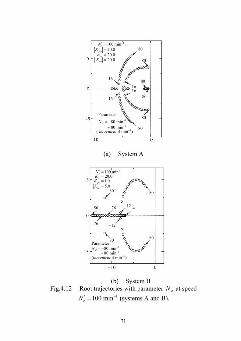
71

* 1100 min20.020.020.0

r

p

sc

i

NK

K

80

80

16

16

16

1680

80

80

80

1

Parameter80 minslN

1( 4 min )increment

1~ 80 min

(a) System A

3

0

3

10 0

8080

80 80

12

Parameter180 minslN

1( 4 min )increment

1~ 80 min

* 1100 min20.01.05.0

r

ic

pc

NKKK

12 456 76

76

(b) System B

Fig.4.12 Root trajectories with parameter slN at speed * 1100 minrN (systems A and B).

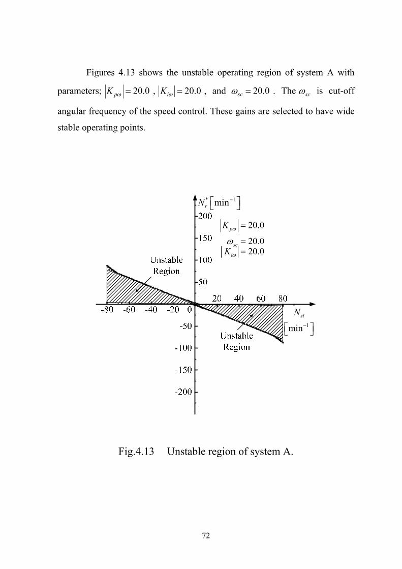
72

Figures 4.13 shows the unstable operating region of system A with

parameters; 20.0pK , 20.0iK , and 20.0sc . The sc is cut-off

angular frequency of the speed control. These gains are selected to have wide

stable operating points.

* 1minrN

20.0

20.020.0

p

sc

i

K

K

1minslN

Fig.4.13 Unstable region of system A.

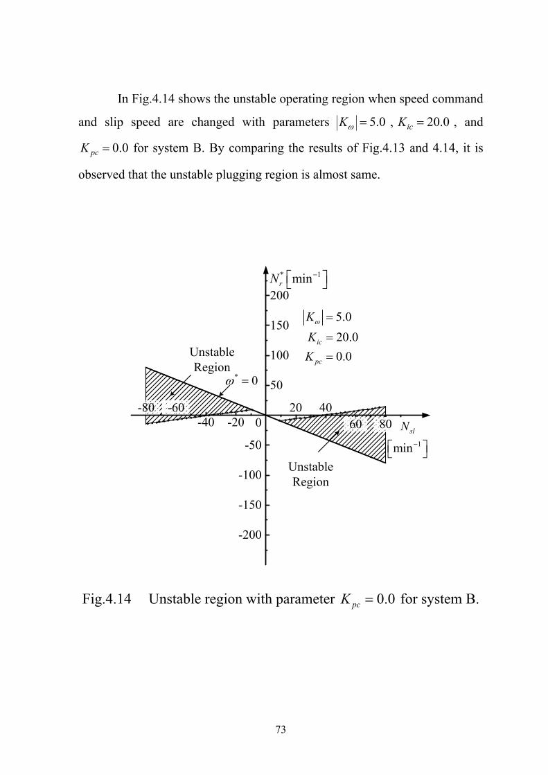
73

In Fig.4.14 shows the unstable operating region when speed command

and slip speed are changed with parameters 5.0K , 20.0icK , and

0.0pcK for system B. By comparing the results of Fig.4.13 and 4.14, it is

observed that the unstable plugging region is almost same.

* 1minrN

5.020.00.0

ic

pc

KKK

-20-40 0

50

100

150

200

4020

-50

-100

-150

-200

-60-8060 80

Unstable Region

Unstable Region

* 0

1minslN

Fig.4.14 Unstable region with parameter 0.0pcK for system B.

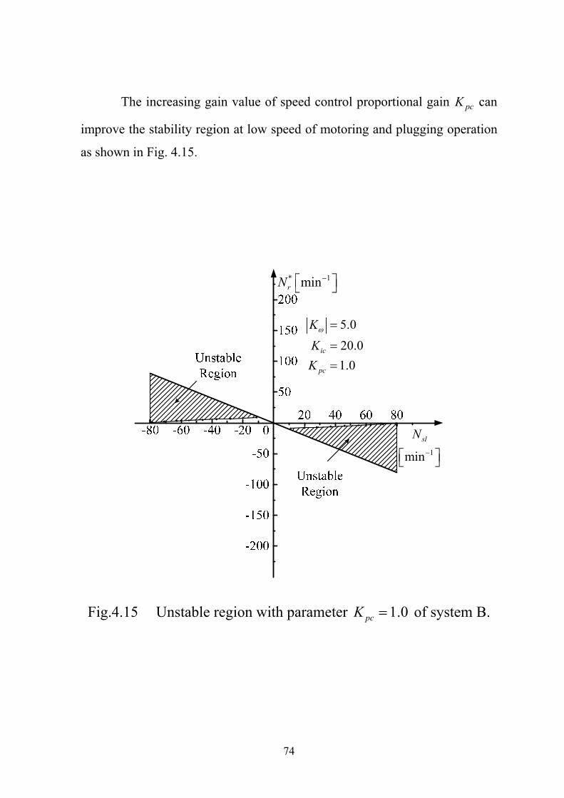
74

The increasing gain value of speed control proportional gain pcK can

improve the stability region at low speed of motoring and plugging operation

as shown in Fig. 4.15.

* 1minrN

5.020.01.0

ic

pc

KKK

1minslN

Fig.4.15 Unstable region with parameter 1.0pcK of system B.

75

4.3 Simulation Results

Figure 4.16 shows the simulation results of non-linear and linear

models of system A. The simulation results of linear and non-linear are

almost same. Therefore, the modeling of the system is appropriate. The

parameters used in this simulations are pK =20.0, iK = 20.0 and sc = 20.0

for system A. In the case of system B, the result is shown in Fig. 4.17. For

system B, the parameters are: K =5.0, icK = 20.0, and pcK =1. The load

torque 4.0 N-mLT is selected.

In Figs.4.18, 4.20 and 4.22, the transient responses of system A and B

are shown for the step change of speed command at motoring operation.

These figures are correspondent to low-speed, medium-speed and high-speed

operations. On the other hand, the transient responses at regenerating

operations are shown in Figs 4.19, 4.21 and 4.23 for low-speed, medium-

speed and high-speed operations respectively.

In system A, the estimated speed ˆr is shown to compare with rotor

speed, while in system B flux frequency * is shown. Both systems A and B

are stable in both regenerating and motoring operations.

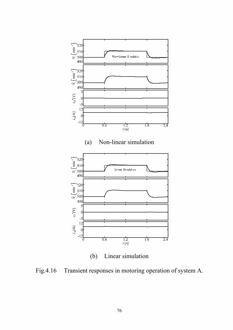
76

-1ˆ

min

rN

-1m

inr

N

(a) Non-linear simulation

-1ˆ

min

rN

-1m

inr

N

(b) Linear simulation

Fig.4.16 Transient responses in motoring operation of system A.

77

[min

-1]

[min

-1]

[V]

[A]

(a) Non-linear simulation

(b) Linear simulation

Fig.4.17 Transient responses in motoring operation of system B.

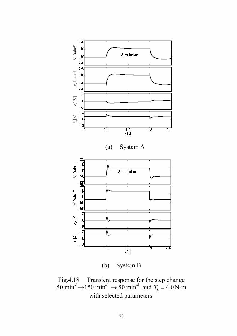
78

e d* [

V]

i sq[A

]ˆ r

Nr

N[m

in-1

][m

in-1

]

(a) System A

*N

rN

(b) System B

Fig.4.18 Transient response for the step change

50 min-1→150 min-1 → 50 min-1 and 4.0LT N-m with selected parameters.

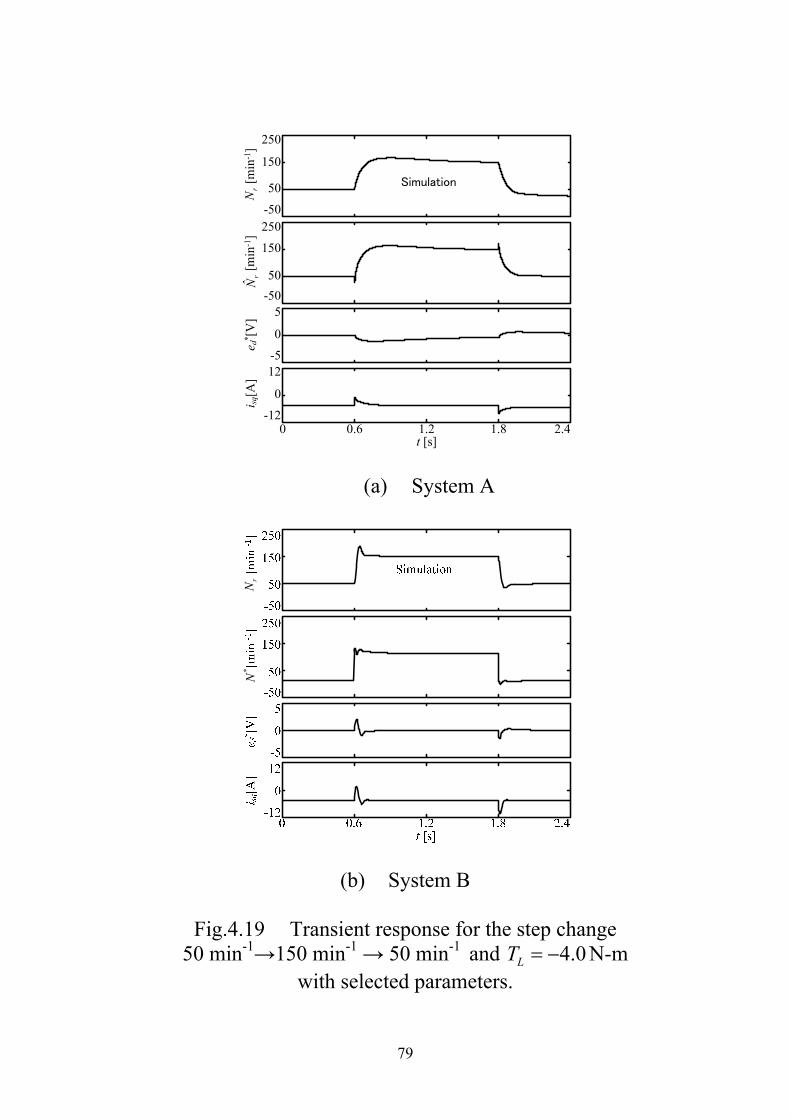
79

t [s]0 0.6 1.2 1.8 2.4

250

e d* [

V]

i sq[A

]

150

50

-50250

150

50-50

5

0

-512

-12

0

ˆ rN

rN

[min

-1]

[min

-1]

Simulation

(a) System A

*N

rN

(b) System B

Fig.4.19 Transient response for the step change

50 min-1→150 min-1 → 50 min-1 and 4.0LT N-m with selected parameters.

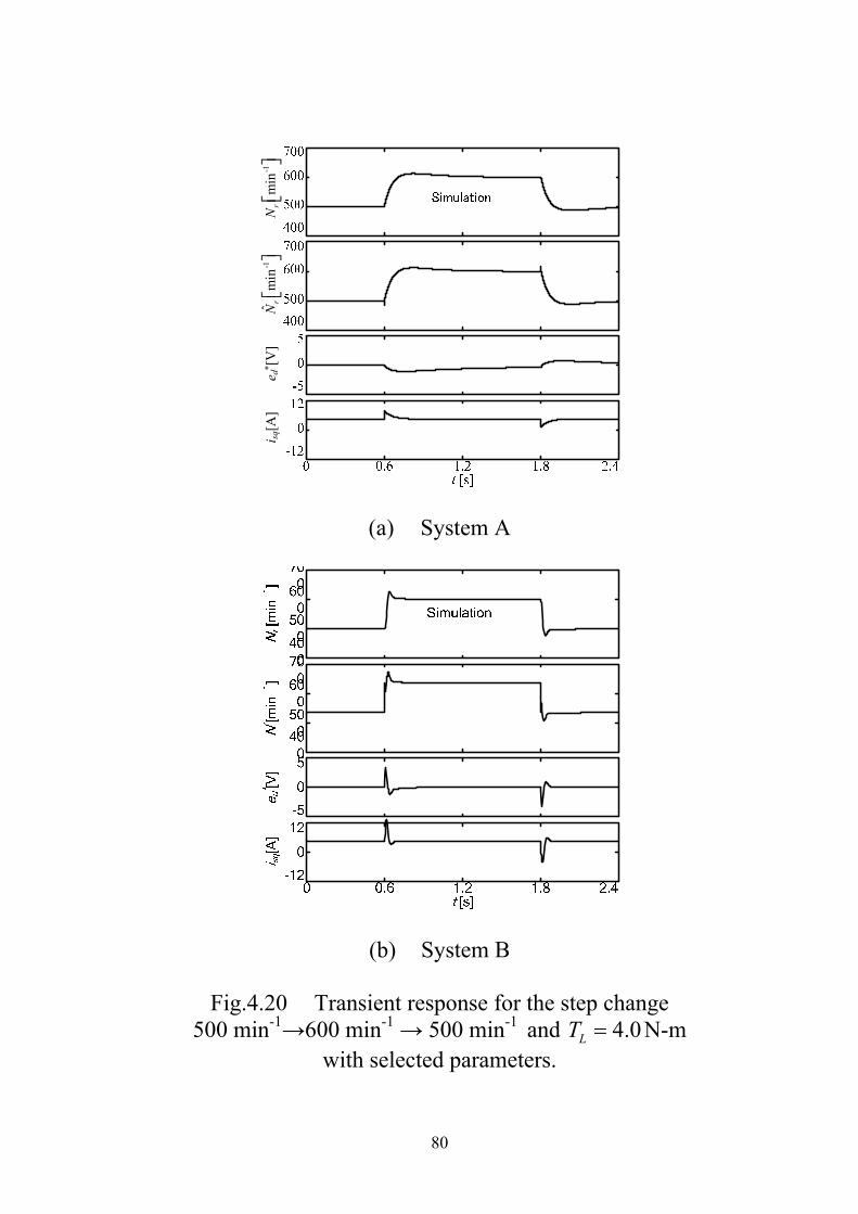
80

e d* [

V]

i sq[A

]-1

ˆm

inr

N

-1

min

rN

(a) System A

(b) System B

Fig.4.20 Transient response for the step change

500 min-1→600 min-1 → 500 min-1 and 4.0LT N-m with selected parameters.

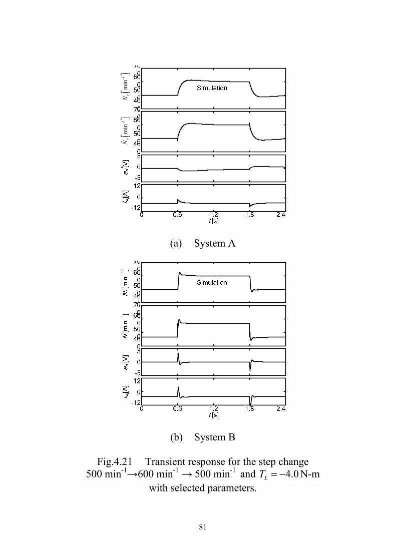
81

-1ˆ

min

rN

-1m

inr

N

(a) System A

(b) System B

Fig.4.21 Transient response for the step change

500 min-1→600 min-1 → 500 min-1 and 4.0LT N-m with selected parameters.

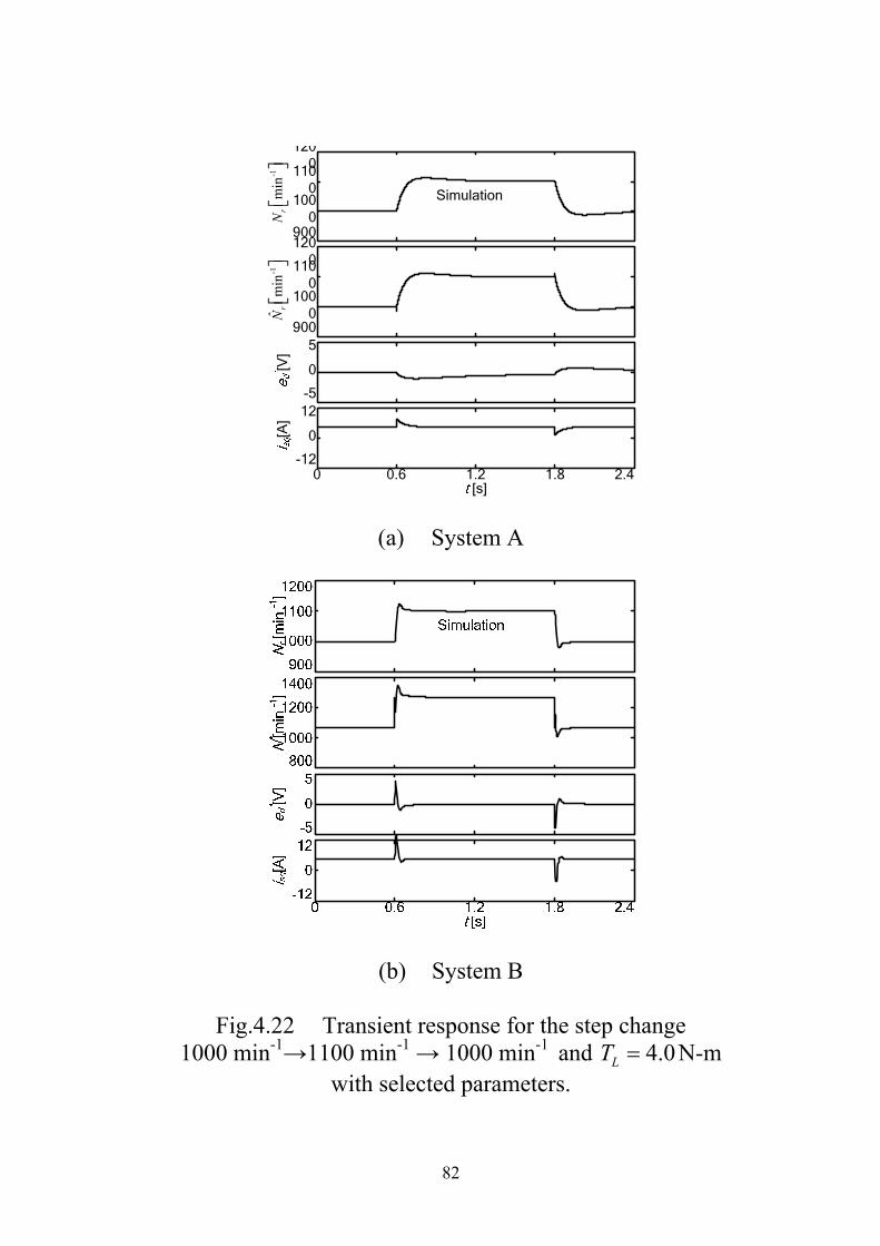
82

1200

[V]

[A]

1100

1000

900120

01100

1000

9005

0

-512

-12

0

-1ˆ

min

rN

-1m

inr

N

[s]0 0.6 1.2 1.8 2.4

Simulation

(a) System A

(b) System B

Fig.4.22 Transient response for the step change

1000 min-1→1100 min-1 → 1000 min-1 and 4.0LT N-m with selected parameters.

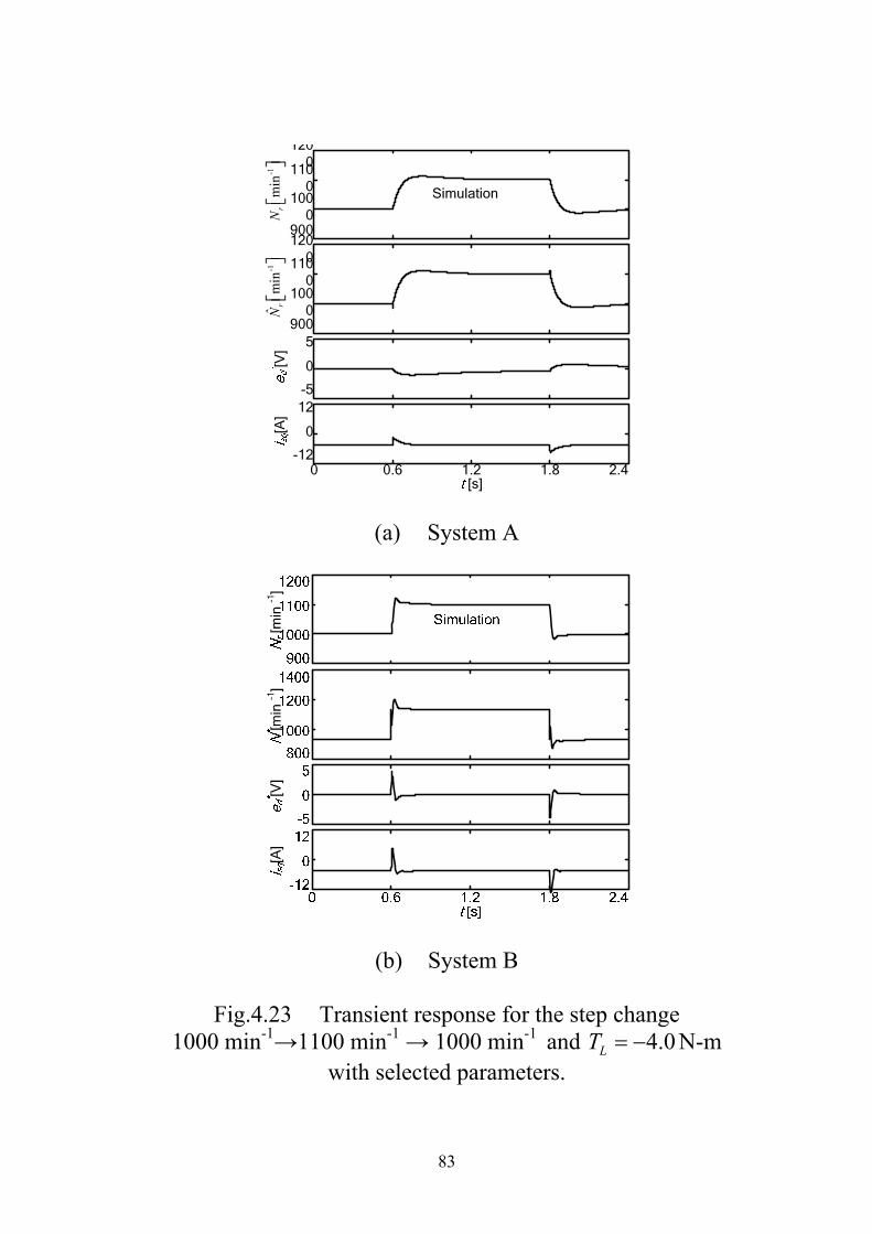
83

[s]0 0.6 1.2 1.8 2.4

1200

[V]

[A]

1100

1000

900120

01100

1000

9005

0

-512

-12

0

-1ˆ

min

rN

-1m

inr

N

Simulation

(a) System A

[min

-1]

[min

-1]

[V]

[A]

(b) System B

Fig.4.23 Transient response for the step change

1000 min-1→1100 min-1 → 1000 min-1 and 4.0LT N-m with selected parameters.

84

4.4 Experimental Results

All experimental results are shown in the case of system B. Figures

4.24, 4.25 and 4.26 shows the simulation and the experimental results for low,

medium and high speed respectively. rN is actual motor speed r and *N

is synchronous speed * . The control parameters are set as 5.0K ,

20.0icK and 0.0pcK . The load torque LT is set to 4.0 N-m (half of rated

torque). From these comparisons, the experimental results are very close to

those of simulation. Therefore, the validity of proposed method is confirmed,

except for high frequency ripples. The high frequency ripples of *N and *de

are caused by PWM voltage control in experimental system. However, since

the flux angle * is obtained by integrating * , the actual rotor speed has

little ripples.

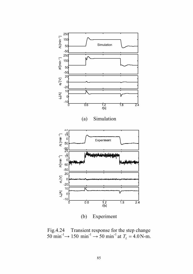
85

250

[min

-1]

[min

-1]

[V]

[A]

150

50

-50250

150

50

-5020

0

-2010

-10

0

[s]0 0.6 1.2 1.8 2.4

Simulation

(a) Simulation

(b) Experiment

Fig.4.24 Transient response for the step change 50 min-1→ 150 min-1 → 50 min-1

at 4.0LT N-m.

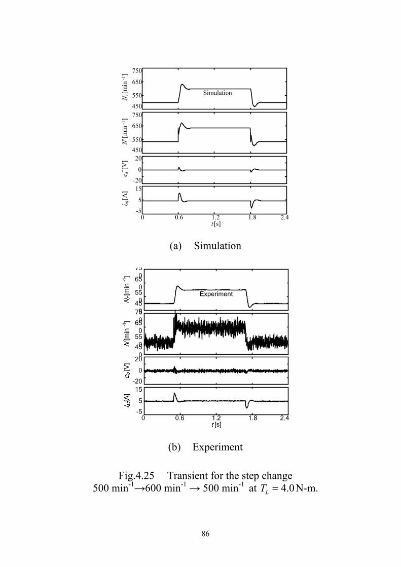
86

750

Nr[

min

-1]

N* [m

in-1

]e d

* [V

]i sq

[A]

650

550450750650

55045020

0-2015

-55

t [s]0 0.6 1.2 1.8 2.4

Simulation

(a) Simulation

[s]0 0.6 1.2 1.8 2.4

750

[min

-1]

[min

-1]

[V]

[A]

650

550450750650

550450

20

0

-2015

-5

5

Experiment

(b) Experiment

Fig.4.25 Transient for the step change 500 min-1→600 min-1 → 500 min-1 at 4.0LT N-m.

87

1400

Nr[

min

-1]

N* [m

in-1

]e d

* [V

]i sq

[A]

1200

1000800

14001200

100080020

0-2015

-55

t [s]0 0.6 1.2 1.8 2.4

Simulation

(a) Simulation

[s]0 0.6 1.2 1.8 2.4

1400

[min

-1]

[min

-1]

[V]

[A]

1200

1000

800140

01200

1000800

20

0

-2015

-5

5

Experiment

(b) Experiment

Fig.4.26 Transient response for the step change 1000 min-1→1100 min-1 → 1000 min-1 at 4.0LT N-m.

88

Figures 4.27, 4.28 and 4.29 shows the simulation and the experimental

result in regenerating operation. Same change of speed command are tested

under the load torque 4.0 N-mLT for low, medium and high speed

respectively. In any cases, quick responses of rN are obtained. The high

frequency ripples of *N in Figs. 4.27, 4.28 and 4.29 are smaller than those in

Figs. 4.24, 4.25 and 4.26. The reason for this difference can be considered

that the amplitude modulation ratio of regenerating operation is smaller if the

voltage control has allowance under limited DC-bus voltage; the distortion of

stator currents is reduced. The larger we choose the gain K , the larger high

frequency ripples of *N are induced.

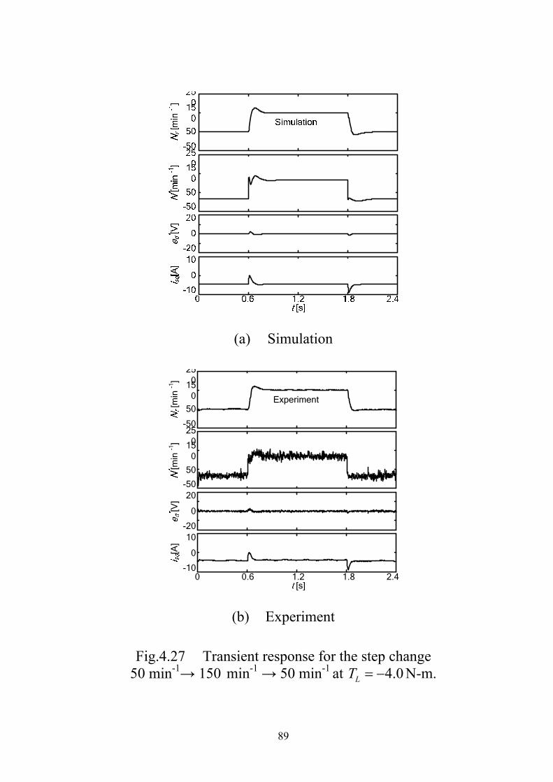
89

(a) Simulation

25

0

[min

-1]

[min

-1]

[V]

[A]

150

50

-5025

0150

50

-5020

0

-2010

-10

0

[s]0 0.6 1.2 1.8 2.4

Experiment

(b) Experiment

Fig.4.27 Transient response for the step change 50 min-1→ 150 min-1 → 50 min-1

at 4.0LT N-m.

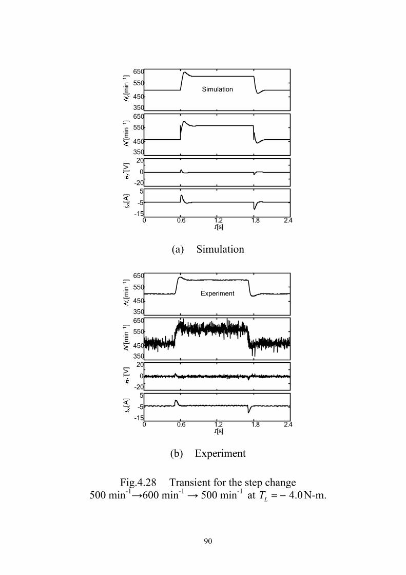
90

650

[min

-1]

[min

-1]

[V]

[A]

550

450

350650

550

450

35020

0

-205

-15

-5

[s]0 0.6 1.2 1.8 2.4

Simulation

(a) Simulation

650

[min

-1]

[min

-1]

[V]

[A]

550

450

350650

550

450

35020

0

-205

-15

-5

[s]0 0.6 1.2 1.8 2.4

Experiment

(b) Experiment

Fig.4.28 Transient for the step change 500 min-1→600 min-1 → 500 min-1 at 4.0LT N-m.

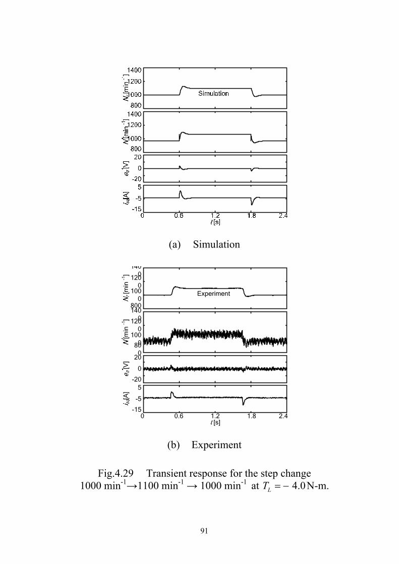
91

(a) Simulation

[s]0 0.6 1.2 1.8 2.4

1400

[min

-1]

[min

-1]

[V]

[A]

1200

1000

800140

01200

1000800

20

0

-205

-15

-5

Experiment

(b) Experiment

Fig.4.29 Transient response for the step change 1000 min-1→1100 min-1 → 1000 min-1 at 4.0LT N-m.

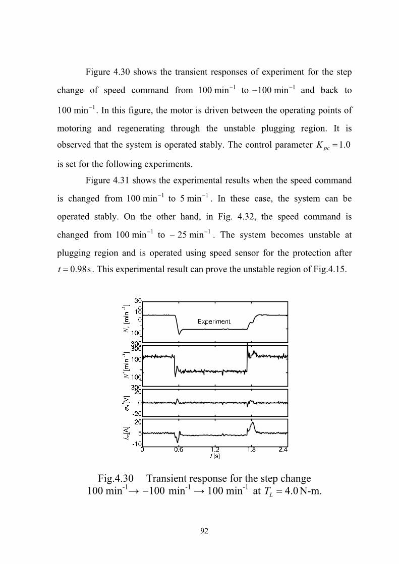
92

Figure 4.30 shows the transient responses of experiment for the step

change of speed command from 1100 min to 1100 min and back to

1100 min . In this figure, the motor is driven between the operating points of

motoring and regenerating through the unstable plugging region. It is

observed that the system is operated stably. The control parameter 1.0pcK

is set for the following experiments.

Figure 4.31 shows the experimental results when the speed command

is changed from 1100 min to 15 min . In these case, the system can be

operated stably. On the other hand, in Fig. 4.32, the speed command is

changed from 1100 min to 125 min . The system becomes unstable at

plugging region and is operated using speed sensor for the protection after

0.98st . This experimental result can prove the unstable region of Fig.4.15.

*N

rN

Fig.4.30 Transient response for the step change

100 min-1→ 100 min-1 → 100 min-1 at 4.0LT N-m.

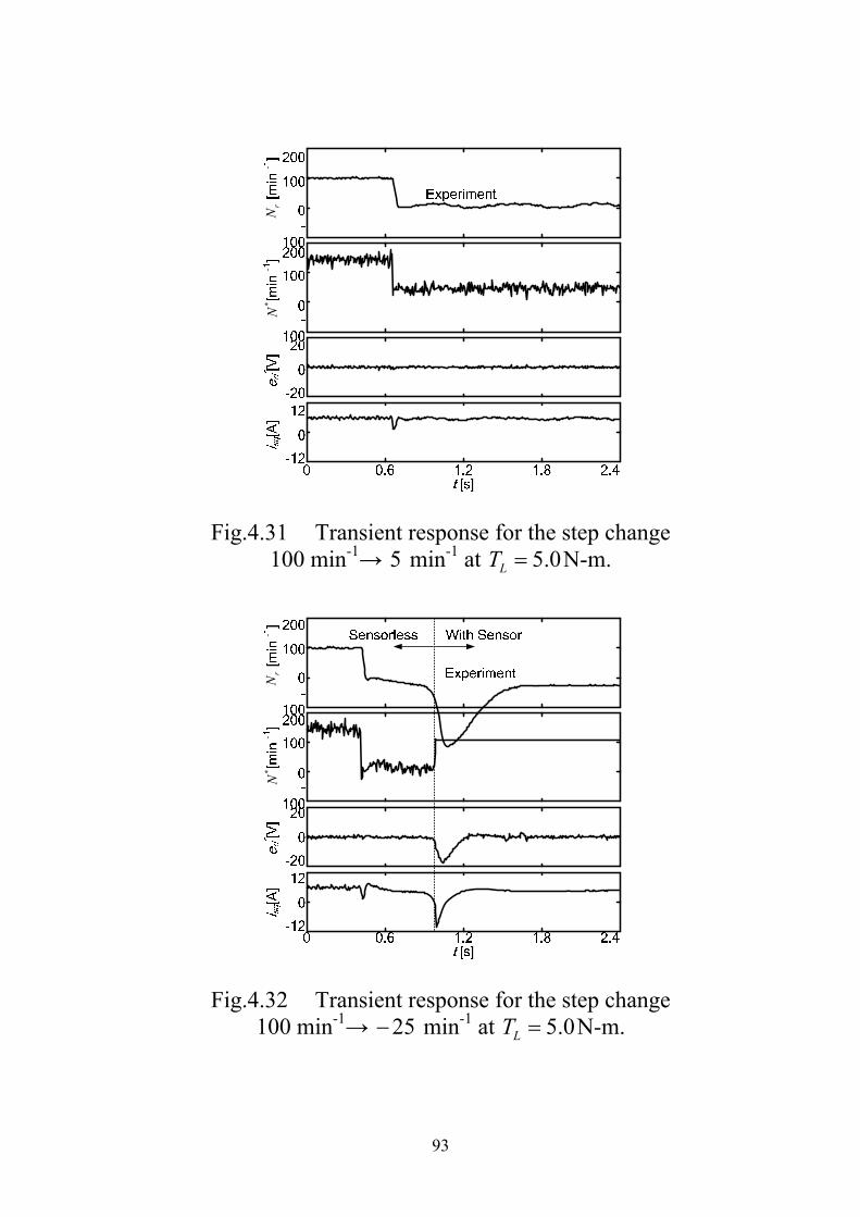
93

*N

rN

Fig.4.31 Transient response for the step change

100 min-1→ 5 min-1 at 5.0LT N-m.

*N

rN

Fig.4.32 Transient response for the step change

100 min-1→ 25 min-1 at 5.0LT N-m.

94

Moreover, Figs.4.33 and 4.34 shows the experimental results for the

step change of the speed command *rN with speed changed 50 min-1→ 150

min-1→ 50 min-1 corresponding to Fig.4.18 (b) and 4.19 (b) in motoring and

regenerating operation respectively. These figures can compare the responses

of actual rotor speed rN for control parameter 1.0pcK .

Figure 4.35 shows the transient response at no-load condition 0LT ,

with speed changed 50 min-1→ 150 min-1→ 50 min-1 corresponding to Figs.

4.33 and 4.34. The speed responses give almost the same characteristics for

each load torque. However, the sqi differs from each parameter of LT .

[min

-1]

[min

-1]

[V]

[A]

*N

rN

Fig.4.33 Transient response for the step change 50 min-1→150 min-1 → 50 min-1 at 4.0LT N-m.

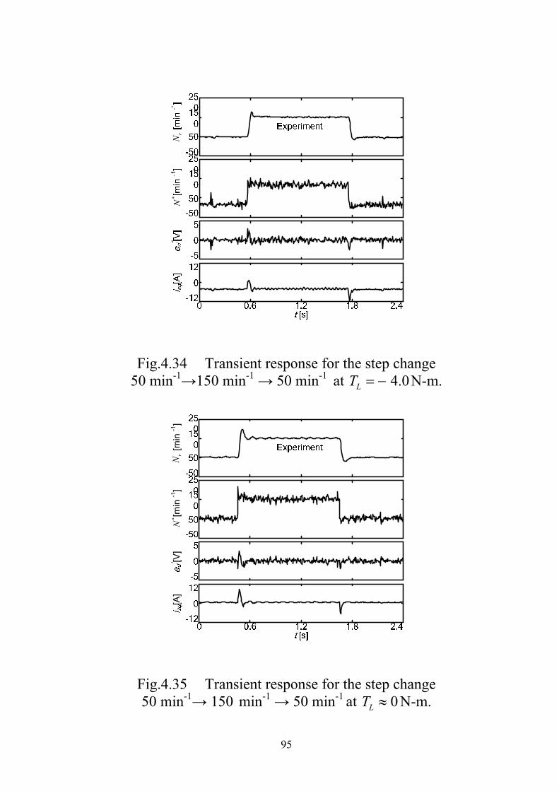
95

*N

rN

Fig.4.34 Transient response for the step change 50 min-1→150 min-1 → 50 min-1 at 4.0LT N-m.

[min

-1]

[min

-1]

[V]

[A]

*N

rN

Fig.4.35 Transient response for the step change 50 min-1→ 150 min-1 → 50 min-1

at 0LT N-m.

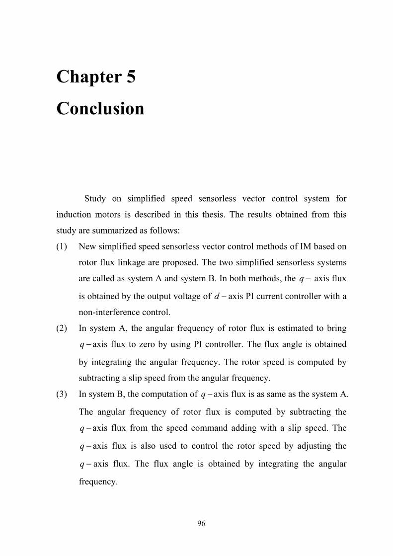
96

Chapter 5

Conclusion

Study on simplified speed sensorless vector control system for

induction motors is described in this thesis. The results obtained from this

study are summarized as follows:

(1) New simplified speed sensorless vector control methods of IM based on

rotor flux linkage are proposed. The two simplified sensorless systems

are called as system A and system B. In both methods, the q axis flux

is obtained by the output voltage of d axis PI current controller with a

non-interference control.

(2) In system A, the angular frequency of rotor flux is estimated to bring

q axis flux to zero by using PI controller. The flux angle is obtained

by integrating the angular frequency. The rotor speed is computed by

subtracting a slip speed from the angular frequency.

(3) In system B, the computation of q axis flux is as same as the system A.

The angular frequency of rotor flux is computed by subtracting the

q axis flux from the speed command adding with a slip speed. The

q axis flux is also used to control the rotor speed by adjusting the

q axis flux. The flux angle is obtained by integrating the angular

frequency.

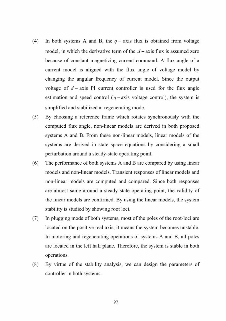
97

(4) In both systems A and B, the q axis flux is obtained from voltage

model, in which the derivative term of the d axis flux is assumed zero

because of constant magnetizing current command. A flux angle of a

current model is aligned with the flux angle of voltage model by

changing the angular frequency of current model. Since the output

voltage of d axis PI current controller is used for the flux angle

estimation and speed control ( q axis voltage control), the system is

simplified and stabilized at regenerating mode.

(5) By choosing a reference frame which rotates synchronously with the

computed flux angle, non-linear models are derived in both proposed

systems A and B. From these non-linear models, linear models of the

systems are derived in state space equations by considering a small

perturbation around a steady-state operating point.

(6) The performance of both systems A and B are compared by using linear

models and non-linear models. Transient responses of linear models and

non-linear models are computed and compared. Since both responses

are almost same around a steady state operating point, the validity of

the linear models are confirmed. By using the linear models, the system

stability is studied by showing root loci.

(7) In plugging mode of both systems, most of the poles of the root-loci are

located on the positive real axis, it means the system becomes unstable.

In motoring and regenerating operations of systems A and B, all poles

are located in the left half plane. Therefore, the system is stable in both

operations.

(8) By virtue of the stability analysis, we can design the parameters of

controller in both systems.

98

(9) A digital signal processor (DSP) based PWM inverter fed IM system is

equipped and tested. It is confirmed that the experimental results are

very close to those of non-linear simulation except for high frequency

ripples. Therefore, the effectiveness of the proposed methods are also

demonstrated experimentally.

(10) The nonlinear simulation and experimental results of the proposed

system show stable and quick transient responses in both motoring and

regenerating modes.

(11) By using PI speed control ( q axis voltage control), the unstable region

is improved comparing with the case of I control in system B.

(12) It is considered that the system B is superior to the system A because its

simple structure in the case of speed control applications.

99

References

[1] C. Schauder, “Adaptive speed identification for vector control of

induction motors without rotational transducers”, IEEE Trans. Ind. Appl.,

vol.28, No.5, pp. 1054–1061 (1992)

[2] H. Tajima, Y. Hori, “Speed sensorless field-orientation control of the

induction machine”, IEEE Trans.Ind. Appl., vol. 29, No.1, pp. 175–180,

(1993)

[3] H. Kubota, K. Matsuse, and T. Nakano “DSP-based speed adaptive flux

observer of induction motor”, IEEE Trans. Ind. Appl., vol.29, No.2, pp.

344–348 (1993)

[4] J. Holtz, “Speed estimation and sensorless control of AC drive”, Conf.

Rec. IEEE-IECON, pp. 649 – 654 (1993)

[5] H. Kubota, K. Matsuse, “Speed sensorless field oriented control of

induction motor with rotor resistance adaptation”, Conf. Rec. IEEE-IAS

Ann. Mtg., pp. 414 – 418 (1993)

[6] T. Kanmachi, I. Takahashi, “Sensorless speed control of an induction

motor with no influence of secondary resistance variation”, Proc.of IEEE

IAS Ann. Mtg., pp. 408 – 413 (1993)

100

[7] M. Tsuji, E. Yamada, K. Izumi and J. Oyama, “A flux observer based

vector control of a controlled current source-fed induction motor”, Trans.

IEE Japan, vol.113-D, No.10, pp.1145 – 1153 (1993)

[8] M. Tsuji, E. Yamada, K. Izumi and J. Oyama, “Stability analysis of a

controlled-current source-fed induction motor vector control system

without a speed sensor”, Electrical Engineering in Japan, vol.114, No.1,

pp.78 – 87 (1994) (in Japanese)

[9] C. Ilas, A. Bettini, L. Ferraris, G. Griva, F. Profumo, “Comparison of

different schemes without shaft sensors for field oriented control drives”,

Proc. of the 20th int. Conf. on Industrial Electronics, Control and

Instrumentation, IEEE-IECON, pp. 1579 – 1588 (1994)

[10] H. Kubota, M. Tsuji, “Online tuning of induction machine parameters”,

National Convention Rec. IEE Japan IAS Symposium, pp.s69 – s74

(1995) (in Japanese)

[11] T. Kanmachi, I. Takahashi, “A secondary resistance calculation method

for sensorless speed control of an induction motor”, Proc. IPEC-

Yokohama’95, pp.1671 – 1676 (1995)

[12] P. K. Kovacs, “Transient phenomena in electrical machine”, Elsevier,

1984

[13] P. C. Krause, “Analysis of electric machinery”, McGraw-Hill Book

Company, 1986

101

[14] P. Vas, “Sensorless vector and direct torque control”, Oxford University

Press, 1998

[15] M. Tsuji, S. Chen, K. Izumi, T. Ohta, E. Yamada, “A speed sensorless

induction motor vector control system using q-axis flux with parameter

identification”, Conf. Rec. IEEE-IECON, pp. 960 – 965 (1997)

[16] M. Tsuji, E. Yamada, F. Parasiliti, M. Tursini, “A digital parameter

identification for a vector controlled induction motor, Proc. of EPE,

pp.4.603 – 4.608 (1997)

[17] J. S. Lee, T. Takeshita, N. Matsui, “Stator-flux oriented sensorless

induction motor drive for optimum low-speed performance”, IEEE Trans.

Ind. Application, vol.33, No.5, pp. 1170 – 1176 (1997)

[18] H. Umida, “The system configuration of speed sensorless vector control”,

Trans. IEE Japan, vol.117-D, No.5, pp.541 – 543 (1997) (in Japanese)

[19] M. Tsuji, S. Doki, “Advanced vector control for accurate torque control”,

National Conv. Rec. IEE Japan IAS, pp.s3 – s8 (1997)

[20] T. Noguchi, S. Kondo, I. Takahashi, “Field-oriented control of an

induction motor with robust online tuning of its parameters”, IEEE Trans.

Ind. Applications, vol.33, No.1, pp.35 – 42 (1997)

102

[21] M. Tsuji, H. Li, K. Izumi, E. Yamada, “A generalized method of

controlled voltage source-fed induction motor vector control using the

observer theory, Electrical Engineering in Japan, vol.119, No.4, pp. 66 –

76 (1997)

[22] H. Kubota, K. Matsuse, and Y. Hori, “Behavior of sensorless induction

motor drives in regenerating mode”, Proc.PCC-Nagaoka’97, pp.549 –

552 (1997)

[23] K. D. Hurst, T. G. Habetler, G. Griva, and F. Profumo, ”Zero-speed

tacholess IM torque control: Simply a matter of stator voltage

integration”, IEEE Trans. Ind. Applicat., vol.34, pp.790 – 795 (1998)

[24] M. Tursini, R. Petrella, and F. Parasiliti, “Adaptive sliding-mode

observer for speed sensorless control of induction motors”, IEEE Trans.

Ind. Appl., vol.36, No.5, pp.1380-1387 (2000)

[25] T. Hamajima, M. Hasegawa, S. Doki, and S. Okuma, “Sensorless vector

control of induction motor with stator resistance identification based on

augmented error”, Proc. of Power Conversion Conf.(PCC-Osaka), pp.

504 - 509 (2002)

[26] S. Suwankawin and S. Sangwongwanich, “A speed-sensorless IM drive

with decoupling control and stability analysis of speed estimation”, IEEE

Trans. Ind. Electron., vol.49, No.2, pp. 444 – 455 (2002)

[27] M. Hinkkanen, “Analysis and design of full-order flux observers for

sensorless induction motors”, IEEE Trans. Ind. Electron., vol.51, No.5,

pp. 1033 – 1040 (2004)

103

[28] M. Hinkkanen and J. Luomi, “Stabilization of regenerating-mode

operation in sensorless induction motor drives by full-order flux observer

design”, IEEE Trans. Ind. Electron., vol.51, No.6, pp. 1318 – 1328

(2004)

[29] M. Saejia and S. Sangwongwanich, “Averaging analysis approach for

stability analysis of speed-sensorless induction motor drives with stator

resistance estimation”, IEEE Trans. Ind. Electron., vol.53, No.1, pp.

162–177 (2006)

[30] C. Lascu, I. Boldea, and F. Blaabjerg, “A class of speed-sensorless

sliding-mode observers for high-performance induction motor drives”,

IEEE Trans. Ind. Electron., vol.56, No.9, pp. 3394–3403 (2009)

[31] L. Harnefors and M. Hinkkanen, “Complete stability of reduced-order

and full-order observers for sensorless IM drives”, IEEE Trans. Ind.

Electron., vol. 55, No.3, pp. 1319 – 1329 (2008)

[32] M. Hinkkanen, L. Harnefors, and J. Luomi, “Reduced-order flux

observer with stator-resistance adaptation for speed sensorless induction

motor drives”, IEEE Trans. Power Electron., vol.25, No.5, pp. 1173–

1183 (2010)

[33] T. Okuyama, N. Fujimoto, H. Fujii, “Simplified vector control system

without speed and voltage sensors – effects of setting errors in control

parameters and their compensation –”, Trans. IEE Japan, vol.110-D, pp.

477 – 486 (1990) (in Japanese)

104

[34] S. Ishida, T. Endo, H. Fujii, H. Tomita, N. Fujimoto, “Sensorless vector

control with quick response for general purpose inverters” Proc. of

Power Conversion Conf. (PCC-Yokohama) pp. 467 – 472 (1993)

[35] H. Tajima, Y. Matsumoto, H. Umida, and M. Kawano, “Speed

sensorless vector control method for an industrial drive system”, Proc. of

International Power Electronics Conference (IPEC-Yokohama) ,

pp.1034–1039 (1995)

[36] K. Kondo and K. Yuki, “Study on an application of induction motor

speed sensorless vector control to railway vehicle traction”, Trans. IEE

Japan, vol.125-D, pp. 1–8 (2005) (in Japanese)

[37] N. Yamamura, K. Aiba, Y. Tsunehiro, “Primary flux control for

induction motor drive”, Trans. IEE Japan, vol.113-D, pp.859 – 864

(1993) (in Japanese)

[38] N. Yamamura, I. Yasuoka, N. Nanato, Y. Tsunehiro, “A method for

improving the performance characteristics of induction motor with

primary flux control”, Trans. IEE Japan, vol.119-D, pp. 371 – 376

(1999) (in Japanese)

[39] M. Tsuji, S. Chen, K. Izumi, and E. Yamada, “A sensorless vector

control system for induction motors using q-axis flux with stator

resistance identification”, IEEE Trans. Ind. Electron., vol.48, No.1, pp.

185–194 (2001)

105

[40] M. Tsuji, S. Chen, T. Kai, S. Hamasaki, “Q-axis flux-based sensorless

vector control of induction motor taking into account iron loss”, IEEJ

Trans. IA, vol.126, No.12, pp.1645–1651 (2006)

[41] M. Tsuji, G. M. C. Mangindaan, Y. Kunizaki, R. Hashimoto and S.

Hamasaki, “A New Simplified Sensorless Speed Control of Induction

Motor using d-axis Voltage”, Proc. of The 15th International Conference

on Electrical Machines and Systems (ICEMS), 6 pages (2012.10)

[42] G. M. C. Mangindaan, M. Tsuji and S. Hamasaki, “Transient

Characteristics of a New Simplified Speed Sensorless Vector Control for

Induction Motors”, Proc. of The 16th International Conference on

Electrical Machines and Systems (ICEMS), 6 pages (2013.10)

[43] M. Tsuji, G. M. Ch. Mangindaan, Y. Kunizaki and S. Hamasaki,

“Simplified Speed-Sensorless Vector Control for Induction Motors and

Stability Analysis”, IEEJ Journal of Industry Applications, Vol.3, No.2,

pp.138 – 145, (2014.3)

[44] G. M. Ch. Mangindaan, M. Tsuji, S. Hamasaki, ”Stability Comparison of

New Simplified Speed Sensorless Vector Control System for Induction

Motors”, Journal of International Conference on Electrical Machines

and Systems, Vol.3. No.2, pp.126 – 131, (2014.6)

[45] H. Sugimoto, M. Koyama, S. Tamai, ”AC Servo System no Riron to

Sekkei no Jissai”, So-Go Den-Shi Syuppan (1990) (in Japanese)

106

Acknowledgment

I used this opportunity to express my gratitude to my supervisor,

Professor Mineo Tsuji, for the supervision and guidance that inspired me to

realize this thesis. His enthusiasm, encouragements have been extremely

helpful. He was always available for my questions and he spent generously

his time. He always advised me to discover the solution while leading me to

the right basic, concept, and perception. My thankful also to Assistant

Professor Shinichi Hamasaki for his contributions, assistance and provision.

I would like to express my honest thank to my committee members of

the dissertation, Professor Tsuyoshi Higuchi and Professor Takahiko

Yamashita for their assessment, instruct and valuable criticism.

I would also like to thank Ms.Yurika Kunizaki for her contribution,

support and guidance.

I received financial support from BPPLN-governmental Higher

Education of the Republic of Indonesia.

Last but not least are my family, my wife Susan Marlein Mambu, my

daughters Keensy Aimee Hendrika Mangindaan and Jeska Queency Javelin

Mangindaan. They are supporting me spiritually all through my life to work

for my Ph.D. in engineering.

Glanny Martial Christiaan Mangindaan

Nagasaki University