Narrow Bracketing and Dominated Choices

Matthew Rabin

and

Georg Weizsäcker1

Abstract

We consider a decisionmaker who "narrowly brackets", i.e. evaluates her decisions

separately. Generalizing an example by Tversky and Kahneman (1981) we show that

if the decisionmaker does not have constant-absolute-risk-averse preferences, there

exists a simple pair of independent binary decisions where she will make a �rst-

order stochastically dominated combination of choices. We also characterize, as a

function of preferences, a lower bound on the monetary cost that can be incurred

due to a single mistake of this kind. Empirically, we conduct a real-stakes laboratory

1Rabin: University of California � Berkeley, 549 Evans Hall, Berkeley, CA 94720-3880, USA, ra-

bin@econ.berkeley.edu. Weizsäcker: London School of Economics, Houghton Street, London, WC2A

2AE, U.K., g.weizsacker@lse.ac.uk. We are grateful to Dan Benjamin, Syngjoo Choi, Erik Eyster,

Thorsten Hens, Michele Piccione, Peter Wakker, Heinrich Weizsäcker, seminar participants at Ams-

terdam, Caltech, Cambridge, Helsinki, IIES Stockholm, IZA Bonn, LSE, Zurich, Harvard, Notting-

ham, NYU, Oxford, Pompeu Fabra, and the LEaF 2006, FUR 2008 and ESSET 2008 conferences,

and especially to Vince Crawford and three anonymous referees for helpful comments, and to Zack

Grossman and Paige Marta Skiba for research assistance. The survey experiment was made possible

by the generous support of TESS (Time-Sharing Experiments in the Social Sciences) and the e¤orts

by the sta¤ of Knowledge Networks. We also thank the ELSE Centre at University College Lon-

don for the generous support of the laboratory experiment, and Rabin thanks the National Science

Foundation (Grants SES-0518758 and SES-0648659) for �nancial support.

experiment replicating Tversky and Kahneman�s original experiment, �nding that

28% of the participants violate dominance. In addition, we conduct a representative

survey among the general U.S. population that asks for hypothetical large-stakes

choices. There we �nd higher proportions of dominated choice combinations. A

statistical model suggests that the average preferences are close to prospect-theory

preferences and that about 89% of people bracket narrowly. Results do not vary much

with the personal characteristics of participants.

Keywords: Lottery choice, narrow framing, representative-sample experi-

ments

JEL Classi�cation: B49

Contact: rabin@econ.berkeley.edu, g.weizsacker@lse.ac.uk

2

A mass of evidence, and the ineluctable logic of choice in a complicated world,

suggests that people �narrowly bracket�: a decisionmaker who faces multiple decisions

tends to choose an option in each case without full regard to the other decisions and

circumstances that she faces. In the context of monetary risk, Tversky and Kahneman

(1981) present an experiment that demonstrates both how powerful this propensity

is, and its clear welfare cost. In their experiment, people narrowly bracket even when

faced with only a pair of independent simple binary decisions that are presented

on the same sheet of paper, and as a result make a combination of choices that is

inconsistent with any reasonable preferences. In our slight reformulation, we present

subjects with the following:

You face the following pair of concurrent decisions. First examine both deci-

sions, then indicate your choices, by circling the corresponding letter. Both

choices will be payo¤ relevant, i.e. the gains and losses will be added to your

overall payment.

Decision (i): Choose between

A. a sure gain of £ 2.40

B. a 25% chance to gain £ 10.00 and a 75% chance to gain £ 0.00.

Decision (ii): Choose between

C. a sure loss of £ 7.50

D. a 75% chance to lose £ 10.00, and a 25% chance to lose £ 0.00.

If, as predicted by Kahneman and Tversky�s (1979) prospect theory, the decision-

maker is risk-averting in gains and risk-seeking in losses and if she applies these

preferences separately to the decisions, then she will tend to choose A and D. This

3

prediction was con�rmed: 60% of Tversky and Kahneman�s (1981) participants chose

A and D with small real stakes, and 73% did so for large hypothetical stakes. But

A and D is �rst-order stochastically dominated: the joint distribution resulting from

the combination of B and C is a 14chance of gaining £ 2.50 and a 3

4chance of losing

£ 7.50; the joint distribution of A and D is a 14chance of gaining £ 2.40 and a 3

4chance

of losing £ 7.60. The BC combination is equal to the AD combination plus a sure

payo¤ of £ 0.10.

In this paper, we explore both the empirical and theoretical generality of this exper-

iment. Our experiments � laboratory experiments both with real and hypothetical

payments, and a hypothetical-payment survey with a representative sample from the

general U.S. population � con�rm the pattern of frequent AD choices, although at

a somewhat lower level. With large hypothetical payo¤s (£ 1 being replaced by £ 100

in the laboratory, and by $100 in the survey) about 60% of participants choose AD;

for small real and hypothetical stakes, 28% and 34% of the subjects do so. We also

introduce three other hypothetical large-stakes sets of decisions where between 40%

and 50% of subjects make dominated choices, despite giving up amounts of $50 and

$75 rather than the $10 in the large-payo¤ version of the original example.

These dominance violations demonstrate that subjects are narrowly bracketing,

because the choice of AD is clearly due to the separate presentation.2 Theoretically,

2A related example of narrow bracketing is Redelmeier and Tversky�s (1992) demonstration that

the investment choice in a risky asset can depend on whether the asset is framed as part of a

portfolio of other assets or as a stand-alone investment. See also the replication and variation in

Langer and Weber (2001), and the literature cited there. Other evidence on narrow bracketing in

lottery choice include Gneezy and Potters (1997) and Thaler et al (1997) who test whether mypoic

loss aversion � a form of narrow bracketing � may serve as a possible explanation of the equity-

premium puzzle, and by Camerer (1989) and Battalio et al (1990), both of whom present treatment

4

we are not aware of any broad-bracketed utility theory ever proposed that would

allow for the choice of AD over BC.3 Empirically, we �nd in a "broad presentation"

treatment, o¤ering an explicit choice between the combinations AC, AD, BC and

BD, that violation rates are reduced to 0% and 6%, respectively, in the laboratory

and the survey.4

The theoretical part of the paper contributes to understanding the generality with

which narrow bracketing can lead to dominated choices. For a given preference rela-

tion � and a given set of choice sets, we de�ne narrow bracketing as the application

of � separately to each choice set. In contrast, a broad bracketer applies � to the set

that comprises all possible choice combinations. This de�nition is widely applicable

and, in particular, a natural connection can be made to arbitrage possibilities. Build-

ing on Diecidue and Wakker (2002), one can use the de�nition of narrow bracketing

to re-phrase de Finetti�s (1974) Dutch-book theorem: for a narrow bracketer who is

variations that suggest narrow bracketing of standard lottery choices. Papers that have explored

the principles of what we call narrow bracketing include Kahneman and Lovallo (1993), Benartzi

and Thaler (1995) and Read, Loewenstein, and Rabin (1999). Other research has found evidence

of violation of dominance due to errors besides narrow bracketing; see, e.g., Birnbaum et al (1992)

and Mellers, Weiss, and Birnbaum (1992).3Even models that allow for dominance violations � such as the disappointment-theory models of

Bell (1985) and Loomes and Sugden (1986), the related �choice-acclimating personal equilibrium�

concept in K½oszegi and Rabin (2007), and the gambling preferences in Diecidue, Schmidt, and

Wakker (2004) � do not permit the preference for AD over BC, since BC is simply AD plus a sure

amount of money.4We examine the broad presentation in three examples in the survey experiment, and the violation

rates are reduced from 66% to 6%, from 40% to 3%, and from 50% to 29%. The surprisingly high

violations of dominance in the last example even under broad presentation are inconsistent with any

hypothesis about choice behavior that we are aware of and we do not understand what motives or

errors were induced by the design of this example.

5

not risk neutral, there exists a series of choices between correlated gambles such that

her combined choice will be dominated by another feasible combination of choice.5

Being a narrow bracketer, she ignores all correlations between gambles that appear in

di¤erent choices and thus she can be tricked into a suboptimal combination. In light

of this, Tversky and Kahneman�s example is is striking in that it works even if the

gambles are uncorrelated. Hence, even if a decisionmaker merely ignores other un-

correlated choices, prospect-theory preferences may induce her to choose a �rst-order

stochastically dominated portfolio.6 This extension is not trivial: most prospects in

life are relatively independent of each other and it is a considerably weaker assump-

tion that people ignore only independent background choices. Moreover, the example

induces dominance in only two binary decisions.

Yet we show below that Tversky and Kahneman�s example can itself be generalized

considerably. The main result in Section 1 establishes that the logic of their exam-

ple extends broadly beyond prospect-theoretic preferences: if a narrow bracketer�s

risk attitudes are not identical at all possible ranges of outcomes � essentially, if

she does not have constant-absolute-risk-aversion (CARA) preferences � then there

exists a pair of independent binary lottery problems where she chooses a dominated

combination.

The logic behind this simple result is itself simple. In the Tversky and Kahneman

example, narrow bracketing means that a prospect-theoretic chooser takes a less-

than-expected-value certain amount over the lottery in the gain domain due to risk

aversion, but takes the lottery over its expected value in the loss domain due to risk-

lovingness. Since her payo¤ is the sum of the two gambles, she�d be better o¤ doing

5The result is the single-person analogue of the fundamental theorem of asset pricing, which

equates the market�s freedom from arbitrage with as-if risk neutrality of prices.6Our instructions made clear that all draws are independent.

6

the opposite. But the potential for dominance does not depend on where or how her

risk attitudes di¤er: if a person�s absolute risk aversion is not identical over all possible

ranges, then there exists a non-risky alternative payment that a person would prefer

to a given lottery in one range that involves sacri�cing more money than a non-risky

payment that she would reject in favor of the same lottery in another range. If o¤ered

both decisions between such non-risky payments and the corresponding lotteries, a

narrow bracketer will therefore choose the non-risky alternative only in the case where

it involves more sacri�ce. But then reversing her choices leaves her with the same

risk but a higher distribution of outcomes.

This result relies solely on monotonicity and completeness of preferences as well

as the existence of certainty equivalents. In particular, it does not assume that the

decisionmaker is an expected-utility maximizer in the sense of weighting prospects

linearly in probabilities. Section 1 also establishes two stronger results for the case of

linear-in-probability evaluations. First, we characterize as a function of preferences a

lower bound on the maximum amount that the decisionmaker can leave on the table

in only two choices, establishing that a narrow bracketer with preferences signi�cantly

di¤erent from CARA can be made to give up substantial amounts of money in such

cases. Second, we show that a pair of independent binary choices can induce domi-

nance even for a decisionmaker who has an arbitrarily small propensity to narrowly

bracket.

While our results establish the existence of situations that generate dominance

violations, we do not address the empirical prevalence of such situations or scale of

welfare loss from dominated choices.7 However, a narrow bracketer who faces a large

7Also, we take as given the perception of what is in each bracket and do not discuss the origin of

narrow bracketing.

7

enough set of varied decisions will make a dominated choice overall if only one pair

of those decisions generates a dominated choice. And people will typically lose utility

from bracketing narrowly even when they do not violate dominance; we focus on

dominance violations because they are suboptimal for all monotonic preferences.

The high rates of dominance violations in the experiments indicate directly that

many subjects are not broad-bracketing utility maximizers. But to demonstrate that

narrow-bracketing utility maximization has greater explanatory power, we use a sim-

ple statistical model to jointly estimate the subjects�utility and the extent of narrow

bracketing. Agents are all assumed to maximize a common utility function, but to

di¤er as to whether they bracket narrowly or broadly. We estimate that about 89% of

decisions are made with narrow brackets, and that average preferences accord to the

prospect-theory value function, with risk aversion in gains and around the status quo

point, and a preference for risk in losses. While the estimation strategy comes with

strong assumptions � most notably, that preferences are homogeneous across the

population � Section 3 provides additional statistics that robustly indicate narrow

bracketing.

The data on personal characteristics in our survey sample also allows us to ask

who brackets narrowly. We �nd few strong correlations of bracketing propensity with

observable background characteristics. In each of the subgroups that we examined,

between 0% and 22% of people are broad bracketers, with few signi�cant deviations

from the average level of 11%. There is more variation, however, in estimated prefer-

ences. �Non-white�respondents are more risk-neutral with respect to lotteries around

zero and in the gains domain, which makes them less likely to violate dominance. Al-

though less pronounced, estimates also suggest that men are more risk neutral than

women and that the math-skilled are more risk neutral than the less math-skilled

8

respondents. Perhaps surprisingly, we �nd no signi�cant e¤ect of education on the

violation rates.

Although this paper concentrates on the �positive� questions of when and how

narrow bracketing leads people to dominated choice, we elaborate in Section 4 on

the implications our analysis has for the normative status of various models of risky

choice. We then conclude the paper with a brief discussion of whether such violations

may be observed in markets where agents interact, and with some methodological

implications for assessments of risk preferences. Our Appendix presents proofs, and

more detail on our experimental procedures and results are on the journal�s Web site.

1 Theory

Assume that a person simultaeneously faces I di¤erent choice sets M1; :::;MI , where

every possible mi 2 Mi induces a lottery, or probability distribution, Li(xijmi) over

changes in wealth xi 2 R. A possible vector of choices m = (m1; :::;mI) induces

a probability distribution over the sum of wealth changes xI =Xi

xi, denoted by

F (xI jm). We restrict attention to the case that the lotteries Li are independent

across the "brackets" i = 1; :::; I, and will state conditions for which there exists a set

of choice sets fM1; :::;MIg such that the chosen distribution F (xI jm) is dominated.

As described in the introduction, we denote the decisionmaker�s preferences by �

and de�ne her as a narrow bracketer if she applies � separately to each of the I choice

sets, without consideration to the fact that the relevant outcome is the combined

outcome from all her choices. That is, she chooses from each Mi by evaluating the

lotteries Li(xijmi), but not the summed distribution F (xI jm). We assume further

that � is complete and strictly monotonic over the set of all possible lotteries, and

that according to �, certainty equivalents exist for all available lotteries. Because

9

preferences are monotonic, the agent will never choose a dominated lottery within

any single bracket � but the resulting distribution F (xI jm) may be dominated.

To de�ne the size of a �rst-order stochastic dominance (FOSD) violation, we say

that F1 dominates F2 by an amount � if it holds for all x in their support that

F1(x+�) � F2(x). This measure has a straightforward interpretation: if F1 dominates

F2 by an amount �, any decisionmaker with monotonic preferences will �nd F1 at least

as desirable as receiving F2 plus a sure payment of �. We say that the decisionmaker

violates FOSD by an amount � if she chooses a distribution F2 that is FOS-dominated

by amount � by another available distribution F1.

The propositions below establish that lower bounds for the largest possible � are

linked to the decisionmaker�s variability of risk attitudes, which can be captured by

describing certainty equivalents and their variability. Let CEL be the decisionmaker�s

certainty equivalent for L. Denote by eL� L+4x a lottery that is generated by adding4x to all payo¤s in L, keeping the probabilities constant: eL is a shifted version of L.Finally, de�ne the decisionmaker�s risk premium for lottery L, �L, as the di¤erence

between the lottery�s expected value, �L, and its certainty equivalent: �L = �L�CEL:

A larger �L corresponds to more risk aversion towards L, and the agent is risk neutral

if �L = 0.

Proposition 1 shows that a decisionmaker will violate dominance in joint decisions

to the degree that a shift can induce a change in the risk premium:

Proposition 1: Suppose that the decisionmaker is a narrow bracketer

and there exist a lottery L and a shifted version thereof, eL = L + 4x,

such that j�L � �eLj > �. Then there exists a pair of independent binarychoices such that the decisionmaker violates FOSD by the amount �.

The proof of Proposition 1 follows the logic behind Tversky and Kahneman�s ex-

10

ample. But whereas they applied prospect theory to generate a shift in lotteries (from

D to B) that moved the decisionmaker from risk seeking to risk averse, the proposi-

tion clari�es that neither a sign change in risk aversion nor the type of lottery that

Tversky and Kahneman used is necessary to generate dominance. The construction

works whenever the risk premium changes by any amount, and for any shift of any

lottery. Therefore, dominance can result from narrow bracketing for all but a very

restricted class of preferences. In particular, among all expected-utility preferences,

the proposition shows that a dominance violation is possible for all utility functions

v outside the constant-absolute-risk-aversion family, i.e. any preferences that cannot

be represented by v(x) = CARA(x; �; �; r) � � � � exp(�rx) for any (�; �; r) 2 R3.

This is because under expected utility (and indeed more generally) the CARA family

encompasses exactly those utility functions where the risk premium is constant for

all shifts of all lotteries L. But the proof of Proposition 1 does not rely on prefer-

ences being EU-representable, and hence the violations can occur even for a large

class of non-EU preferences � in particular, preferences that are representable under

probability weighting formulations.

For any given �, however, Proposition 1 is silent about the set of preferences for

which there is a pair of lotteries L and eL with the property j�L � �eLj > �. To in-

vestigate when the decisionmaker is in danger of making a large mistake, we now

consider preferences that are EU-representable by a (possibly reference-dependent)

strictly increasing and continuously di¤erentiable function v whose expected value

she maximizes. This allows us to characterize a lower bound for the size of possi-

ble dominance violations by comparing preferences to the CARA family using the

following metric:

11

De�nition: For an interval [x; x] � R of changes in wealth,

K(v; x; x) � inf(�;�;r)2R3

maxy2[v(x);v(x)]

jv�1(y)� CARA�1(y; �; �; r)j

is the horizontal distance between v and the family of CARA functions.

That is, for an interval [x; x], K is the smallest distance in horizontal direction

such that all CARA functions reach at least this distance from v, somewhere on the

interval. K is a monetary amount that indicates the change in risk attitudes across

di¤erent ranges within [x; x], as CARA represents a constant risk attitude and K

measures the distance between v and CARA. (K�s arguments v; x; x are suppressed

from here onwards.) We can now state another simple proposition (although with a

long proof):

Proposition 2: Suppose that the decisionmaker is a narrow bracketer

and that preferences are EU-representable by a function v that is strictly

increasing and continuously di¤erentiable and has a horizontal distance

of K from the CARA family on the interval [x; x]. Then for all � > 0

there exists a pair of independent binary choices � each between a binary

lottery and a sure payment, and using only payo¤s in [x; x] � such that

the decisionmaker violates FOSD by an amount greater than K � �.

Proposition 2 shows that one can �nd an example where narrow bracketing causes

the decisionmaker to leave K on the table. The proof provides a construction of

two candidate binary lotteries LA and LB, where at least one of them can always be

shifted in a way that yields a variation of the risk premium by K. Hence, Proposition

1 can be applied to generate the violation.

K is de�ned conditional not only on v, but also on the interval [x; x]. If the

interval is expanded, K increases. Indeed, with almost all functional forms of v that

12

are commonly used, such as a two-part linear function or a constant relative risk

aversion function, K becomes in�nitely large as the interval increases to in�nite size.

This is a strong limiting result, but we note that for larger and larger payo¤ sizes the

assumption of narrow bracketing is arguably less and less plausible.

Our �nal theoretical result shows that it is not only fully narrow bracketers who

make dominated choices. To formulate the sense in which "partial narrow bracketing"

causes problems, we abandon our simple de�nition of narrow bracketing, and impose

some additional structure on the preferences. A convenient formulation is the global-

plus-local functional form of Barberis and Huang (2004) and Barberis, Huang and

Thaler (2006): assume that the agent�s choices are determined by maximizing, over

possible choice vectors m, the expression

U(m) = �

Zu(xI)dF (xI jm) + (1� �)

Xi

Zu(xi)dLi(xijmi).

Here u is a valuation function for money, which the decisionmaker applies both glob-

ally to total earnings � as captured in the �rst term � and locally to each choice set

Mi � as captured in the second term. Notice that each element mi of m enters U in

two ways, by contributing to the distribution F of total wealth changes and through

the narrow evaluation of payo¤s in bracket i alone. The parameter � 2 [0; 1) is the

weight of the global part, so that 1 � � is the degree of narrow bracketing. When

� ! 1, choices correspond to fully broad bracketing, and when � = 0, there is fully

narrow bracketing. The proposition shows that if u is di¤erent from CARA, then

an arbitrarily mild degree of narrow bracketing puts the decisionmaker in danger of

FOSD violations: � could be arbitrarily close to 1.8

8The proof in the appendix covers a somewhat stronger statement, allowing for di¤erent valuation

functions in the broad versus narrow parts of the valuations. That is, the proposition holds even if

the function representing the broad valuation (here, �u) is CARA. It su¢ ces if the narrow valuation

13

Proposition 3: Suppose that the decisionmaker maximizes U(�), where u

is strictly increasing, twice continuously di¤erentiable and not a member

of the CARA family of functions. Then there is a pair of independent

binary choices, each between a 50/50 lottery and a sure payment, where

the decisionmaker violates FOSD.

All three propositions highlight that departures from constant absolute risk aversion

lead to dominance violations. In fact, the converse of all propositions is also true:

a person with CARA preferences will never make dominated choices, as even under

broad bracketing her choice within each bracket is independent of the background risk

generated in other brackets. Among economists, there is widespread agreement that

CARA is not the best-�tting class of preferences. To the extent that this agreement

is based on data analyses, however, it is important to note that all estimates of risk

attitudes will crucially depend on the maintained assumptions about bracketing.9 We

are not aware of a study that simultaneously describes risk attitudes and narrowness

of bracketing, and will provide such an estimation in the following sections.

2 Experimental Design and Procedure

We conducted two experiments in di¤erent formats: one laboratory experiment that

replicates and systematically varies the Tversky and Kahneman experiment ("Exam-

ple 1", hereafter), and one survey experiment with a large and representative subject

function (here, (1� �)u) di¤ers from CARA.9The evidence on lottery choice behavior points at a decreasing degree of absolute risk aversion,

for the average decisionmaker � see e.g. Holt and Laury (2002) for laboratory evidence. As in most

related studies, this stylized result implicitly assumes narrow bracketing in the sense that all income

from outside the experiment is ignored in the analysis. Dohmen et al (2005), in contrast, measure

risk aversion also under the assumption that people integrate other assets.

14

pool, where we introduce additional tasks. We describe the procedures of both ex-

periments before describing the additional choice tasks and the data.

2.1 Procedure of the Laboratory Experiment

For the laboratory experiment, 190 individuals (mostly students) were recruited from

the subject pool of the ELSE laboratory at University College London. We held 15

sessions of sizes ranging between 7 and 18 participants, in four di¤erent treatments.

Each participant faced one treatment only, consisting of one particular variant of the

A=B=C=D choices of Example 1. The wording was as given in the introduction.

In the �rst treatment, "Incentives-Small Scale", which was conducted in four ses-

sions with N = 53 participants in total, we used the payo¤s that were given in the

introduction, and these payments were made for real. In a "Flat Fee-Small Scale"

treatment (three sessions, N = 44), participants made the same two choices A=B and

C=D, but only the show-up fee was paid, as explained below. In the third treatment,

"Incentives-Small Scale-Broad Presentation" (four sessions, N = 45), they made only

one four-way decision, choosing between the distributions of the sum of earnings that

would result from the four possible combinations of A and C, A and D, B and C,

and B and D. That is, in this treatment we imposed a broad view by adding up

the payo¤s from the two decisions. For example, the combination of A and D would

be presented as "a 25% chance to gain £ 2.40 and a 75% chance to lose £ 7.60."10

Finally, in a "Flat Fee-Large Scale" treatment (three sessions, N = 48), the partici-

pants made the two hypothetical choices of the second treatment, but we multiplied

all payo¤ numbers by a factor of 100. Hence, they could make hypothetical gains and

10In this treatment, the order of the four choice options was randomly changed between the

participants. In the three treatments with two binary choices, we maintained the same order as in

Tversky and Kahneman (1981).

15

losses of up to £ 1000 in this treatment.

On the �rst sheet of the experimental instructions, it was clari�ed that all random

draws in the course of the experiment would be determined by independent coin �ips.

All choices were made by paper and pencil, with only very few oral announcements

that followed a �xed protocol for all treatments, and with the same experimenter

present in all sessions. After the choices on Example 1, the experiments moved on to

a second part. This second part is not analyzed in the paper; the tasks and data are

described in Online Appendix 1. The tasks of the second part di¤ered between the 15

sessions, but the participants were not made aware of the contents of the second part

before making their choices in the �rst part, so that the Example 1 choices cannot

have been a¤ected by the di¤erences in the second part. The participants also had

to �ll in a questionnaire and a sheet with �ve mathematical problems. Finally, the

relevant random draws were made and the participants were paid in cash. The entire

procedure, including payments, took about 40-50 minutes in each session.

An email was sent to the participants 24 hours before the session in which they

participated, and made them aware that (i) they would receive a show-up fee of

£ 22, (ii) that they "may" make gains and losses relative to their show-up fee, and

(iii) that overall, they would be "about equally likely to make gains as losses (on

top of the £ 22)."11 Upon arrival at the laboratory, the participants learned whether

the experiment used monetary incentives or not, i.e. whether the outcome amounts

were added to/subtracted from their show-up fee. This procedure aims at minimizing

possible e¤ects of earnings di¤erences between treatments with hypothetical and real

payments, by ruling out both ex-ante di¤erences and anticipated ex-post di¤erences

in average earnings. In those sessions where we used real monetary incentives, the

11The email text and complete instructions of all experiments are in Online Appendix 3.

16

second part of the experiment was designed such that the expected average of total

earnings would indeed be at £ 22. (On average, the subjects received £ 21.85 in these

sessions, with a standard deviation of £ 7.70.) A further role of the 24-hour advance

notice about the show-up fee was to make the losses more akin to real losses, as the

participants may have "banked" the show-up fee. The amount £ 22 was not mentioned

on the day of the experiment before the subjects had made their Example 1 choices,

and all gains and losses were presented using the words "gain" and "lose".

Treatment # of obs. Sessions

Incentives-Small Scale 53 1-4

Flat Fee-Small Scale 44 5-7

Incentives-Small Scale-Broad Presentation 45 8-11

Flat Fee-Large Scale 48 12-15

Table 1: Overview of laboratory treatments.

2.2 Procedure of the Survey Experiment

The survey experiment used the survey tool of TESS (Time-Sharing Experiments in

the Social Sciences), which regularly conducts questionnaire surveys with a strati�ed

sample of American households, those on the Knowledge Networks panel. The panel

members were recruited based on their telephone directory entries and are used to

answering questions via special TV-connected terminals at their homes. For each

new study, they are contacted by email. In the case of our questionnaire, a total

of 1910 panel members were contacted, of whom 1292 fully completed the study. A

further 30 respondents participated but left at least one question unanswered. (We

included their responses in the analysis, wherever possible.) Each participant was

presented with one or several decision tasks, plus a short questionnaire that asked for

information on mathematics education and gave the participants three mathemati-

17

cal problems to solve. The data set also contains information on each participant�s

personal background characteristics such as gender, employment status, income and

obtained level of education. None of the lotteries was paid out, i.e. all choices were

hypothetical. The amounts used in the decision tasks ranged from �$1550 to +$2500.

In addition to the binary lottery choices that we report here, subjects were also

asked to state certainty equivalents for 11 di¤erent lotteries. In Online Appendix 2, we

describe the procedure and data, and discuss why we feel that these certainty equiva-

lence data are unreliable, as many participants cannot plausibly have understood the

procedure. We therefore do not include these data in the analysis.

Participants were randomly assigned to 10 di¤erent treatment groups, and each

treatment contained a di¤erent set of one, two or six decision tasks (including lot-

tery choices and certainty equivalent statements). Within each decision, the order in

which the choice options appeared was randomized. After excluding two treatments

where only certainty-equivalent statements were collected, the sample contains 2543

choices made by 1130 participants in 8 treatments. Table 2 summarizes the lottery

choice (LC) tasks in each of the 8 treatments and lists the number of certainty equiv-

alent (CE) tasks in the same treatments. Further details on the lottery choice tasks

(Example 1 etc.) are given in the next subsection.

In each treatment, the participants�interfaces forced them to read through all their

decisions before they could make their choices. Importantly, the instructions stated

clearly on the �rst screen that the participants should make their choices as if all

of their outcomes were paid. Hence, it is unlikely that choices were made under

a misunderstanding that only subsets of the decisions were relevant. Also, as in

the laboratory experiment, the instructions made clear that all random draws were

independent.

18

Treatment # of obs. # of LC tasks Description # of CE tasks

1 88 2 Example 1 0

2 86 1 Example 1 � broad presentation 0

3 107 2 Example 2 0

4 108 1 Example 2 � broad presentation 0

5 168 3Example 2

Example 4 � broad presentation3

6 185 3Example 2 � separate screens

Example 33

7 174 2 Example 4 4

8 184 3Example 2 � broad presentation

Example 4 � separate screens3

Table 2: Overview of survey experiment treatments

2.3 The Lottery Choice Problems

The lottery choice tasks of the survey experiment are similar to those in Tversky and

Kahneman�s example, but with a slightly di¤erent wording. Our �rst set of decisions

is parallel to the original example, but using U.S. dollars instead of pounds:

Example 1:

Decision 1: Choose between:

A. winning $240

B. a 25% chance of winning $1000 and a 75% chance of not winning or losing any money

Before answering, read the next decision.

Decision 2: Choose between:

C. losing $750

D. a 75% chance of losing $1000, and a 25% chance of not winning or losing any money

19

This example was conducted in two treatments, once as described above (Treatment

1) and once in the broad four-way presentation of the four combined choices AC, AD,

BC and BD (Treatment 2), analogous to the third laboratory treatment. In both of

these treatments, the participants made no other choices.

In all other treatments, we used only 50/50 gambles. The following are the new

examples that we designed to generate dominance violations (the labels of choice

options were changed from the instructions, for the sake of the exposition):

Example 2:

Decision 1: Choose between:

A. not winning or losing any money

B. a 50% chance of losing $500 and a 50% chance of winning $600

Before answering, read the next decision.

Decision 2: Choose between:

C. losing $500

D. a 50% chance of losing $1000, and a 50% chance of not winning or losing any money

Example 2 was designed to bring loss aversion into play: if participants weigh losses

heavier than gains, they will tend to choose A over B, and if they are risk seeking in

losses, they will tend to choose D over C. Such a combination is dominated with an

expected loss of $50 relative to the reversed choices. This example, too, was conducted

in isolation � i.e. with no other decisions for the participants � and presented as

stated here (Treatment 3) and presented as a broad four-way choice (Treatment 4). In

addition, the example was presented together with other decisions, in three di¤erent

ways. In Treatment 5, the two decisions appeared on the same screen. In Treatment

6, they appeared on separate screens, with four other tasks appearing in between.

This variation was included to detect potential e¤ects (e.g. distractions) caused by

20

other choices. In Treatment 8, the example was presented as a broad four-way choice

alongside with other decisions.

Similar to Example 1, Example 3 uses possible risk aversion in gains and risk

lovingness in losses.

Example 3:

Decision 1: Choose between:

A. winning $1500

B. a 50% chance of winning $1000, and a 50% chance of winning $2100

Before answering, read the next decision. [...]

Decision 2: Choose between:

C. losing $500

D. a 50% chance of losing $1000, and a 50% chance of not winning or losing any money

The choice of A and D is dominated with a loss of $50 on average. The example

was only conducted as stated here, in Treatment 6.12 An important new feature of the

example is that all possible combined outcomes involve positive amounts. Therefore,

although a narrow evaluation of the second decision would consider negative payo¤s,

a broad-bracketing decisionmaker�s choices can only be in�uenced by preferences over

gains. In particular, under the assumption of broad-bracketed choice, a decision for

D over C would be evidence of risk-lovingness in gains.13

12In treatment 6, the second decision of Example 3 is also the second decision of Example 2, so

that the occurences of dominance violations are correlated between the two examples.13This is true only if Example 3 is viewed separately from the third lottery choice decision in

Treatment 6 (Decision 1 in Example 2). Considering all three decisions, the treatment involves

eight possible choice combinations, only one of which involves a possible loss as only one of its eight

possible outcomes. Hence, the choice of D in Example 3 would still be indicative of a preference for

risk with almost all payo¤s being positive.

21

The �nal example uses a more di¢ cult spread between the payo¤s and it involves

some payo¤s that are not multiples of $100:

Example 4:

Decision 1: Choose between:

A. winning $850

B. a 50% chance of winning $100 and a 50% chance of winning $1600

Before answering, read the second decision.

Decision 2: Choose between:

C. losing $650

D. a 50% chance of losing $1550, and a 50% chance of winning $100

As before, a decisionmaker who rejects the risk in the �rst decision but accepts it in

the second decision (A and D) would violate dominance, here with an expected loss of

$75 relative to B and C. An new feature is that these choices sacri�ce expected value

in the second decision, not in the �rst. This implies that for all broad-bracketing

risk averters the combined choice of A and C would be optimal: it generates the

highest available expected value at no variance. Di¤erent from the other examples,

the prediction for a broad-bracketed risk averter is therefore independent of the exact

nature of her preferences. A further property of the example is that A and C would

be predicted even for some narrow bracketers who have preferences like in prospect

theory, with diminishing sensitivity for larger gains and losses, loss aversion, and

risk aversion/lovingness in the gain/loss domains. This is because the risky choice D

involves a possible gain of $100 so that a prospect-theoretic decisionmaker would only

accept the gamble D if the preference for risk in the loss domain is strong relative to

the e¤ect of loss aversion (which makes her averse to lotteries with payo¤s on both

sides of zero). In particular, the preference for risk in the loss domain needs to be

22

slightly stronger than in the often-used parameterization of Tversky and Kahneman

(1992) �see footnote 17. Under the assumption of narrow bracketing, the example

therefore helps to discriminate between di¤erent plausible degrees of risk lovingness

in the loss domain. The example was conducted in Treatments 5, 7, and 8, with

di¤erences between broad versus narrow presentation, and with and without other

decisions appearing in between the two decisions.

3 Experimental Results

3.1 Results of the Laboratory Experiment

Table 3 lists the frequencies of observing each of the four possible choice combinations

in Example 1, in the four di¤erent laboratory treatments.

Treatment A and C A and D B and C B and D

Incentives-Small Scale 0.21 0.28 0.11 0.40

Flat Fee-Small Scale 0.16 0.34 0.09 0.41

Incentives-Small Scale-Broad Presentation 0.11 0.00 0.38 0.51

Flat Fee-Large Scale 0.15 0.54 0.08 0.23

Table 3: Laboratory choice frequencies in Example 1.

There is little di¤erence between the observed behavior in the �rst two treatments.

No matter whether the outcomes are actually paid or not, about half of the respon-

dents choose the sure gain of A over the lottery B, and slightly more than two thirds

choose the uncertain loss of lottery D over the sure loss in C. This con�rms prospect

theory�s prediction of risk-seeking behavior in the losses domain, but with less clear

evidence of risk aversion in the gain domain.14 The dominance-violating combina-

14The choices in the sessions�second parts also show much risk taking behavior.

23

tion of A and D was chosen by 28 percent and 34 percent of the two treatments�

participants, respectively. The di¤erence in these two frequencies is insigni�cant at

any conventional level (p = 0:346, one-tailed Fisher exact test), i.e. we �nd little

indication that the frequency of dominance violations decreases if the decisions are

paid for real. Similarly, testing for di¤erences in the entire distribution of choices, not

just in the frequency of A and D, we cannot reject the null hypothesis of no di¤er-

ence (p = 0:866, two-tailed Pearson chi-square test). Overall, there is no statistically

signi�cant e¤ect of actually paying the (small-scale) decisions in this data set.

Comparing the Flat Fee-Small Scale treatment with the Flat Fee-Large Scale treat-

ment, the frequencies of the dominated AD combination increases from 34 percent

to 54 percent, which is statistically signi�cant (p = 0:042, one-tailed Fisher exact

test).15

Finally, a comparison between the Incentives-Small Scale treatment and the Incentives-

Small Scale-Broad Presentation treatment suggests a strong e¤ect of narrow bracket-

ing. If the participants have to view the decision problem from a broad perspective,

the number of combined A and D choices goes from 28% to 0% (p < 0:001, one-tailed

Fisher exact test), and also the overall distributions of choices are signi�cantly dif-

ferent (p < 0:001, two-tailed Pearson chi-square test). This clearly indicates that the

subjects did not view the two decisions in the Incentives-Small Scale treatment as a

combined problem.

15But a Pearson chi-square test still supports the hypothesis of identical four-way distributions

of choices between the two treatments (p = 0:221, two-tailed). In light of the signi�cant result of

the Fisher exact test we attribute this failure to reject to the low numbers of observations. In any

case, the results do not indicate that a large (hypothetical) payo¤ scale makes people more likely to

bracket broadly.

24

3.2 Results of the Survey Experiment

3.2.1 Data Summary

Treatment Description A and C A and D B and C B and D

1 Example 1 0.16 0.66 0.03 0.15

2 Example 1 � broad presentation 0.22 0.06 0.24 0.48

3 Example 2 0.24 0.53 0.05 0.19

4 Example 2 � broad presentation 0.09 0.38 0.12 0.41

5Example 2

Example 4 � broad presentation

0.22

0.72

0.53

0.04

0.05

0.13

0.20

0.12

6Example 2 � separate screens,

Example 3

0.26

0.23

0.44

0.50

0.07

0.10

0.23

0.17

7 Example 4 0.35 0.36 0.16 0.13

8Example 2 � broad presentation,

Example 4 � separate screens

0.15

0.33

0.24

0.43

0.24

0.10

0.36

0.14

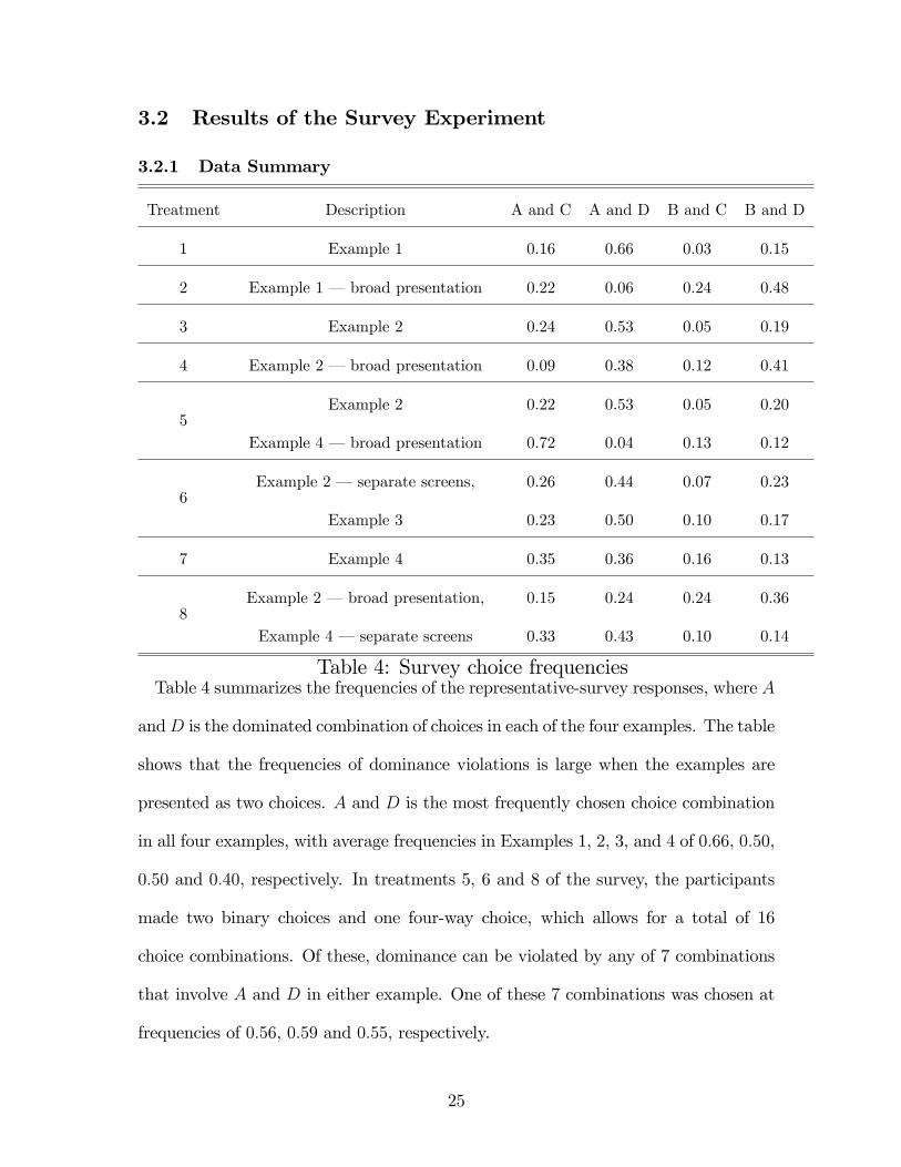
Table 4: Survey choice frequenciesTable 4 summarizes the frequencies of the representative-survey responses, where A

andD is the dominated combination of choices in each of the four examples. The table

shows that the frequencies of dominance violations is large when the examples are

presented as two choices. A and D is the most frequently chosen choice combination

in all four examples, with average frequencies in Examples 1, 2, 3, and 4 of 0:66, 0:50,

0:50 and 0:40, respectively. In treatments 5, 6 and 8 of the survey, the participants

made two binary choices and one four-way choice, which allows for a total of 16

choice combinations. Of these, dominance can be violated by any of 7 combinations

that involve A and D in either example. One of these 7 combinations was chosen at

frequencies of 0:56, 0:59 and 0:55, respectively.

25

All of these observed violations are inconsistent with any model where rational

agents with monotonic preferences make broad-bracketed choices. But the table also

contains more direct evidence against broad bracketing. In the three examples that

we presented broadly, Examples 1, 2 and 4, the frequencies of dominated choice are

signi�cantly reduced. In Examples 1 and 4, violations are reduced drastically, to 0:06

and 0:03, respectively. But in the case of Example 2, there remains a large proportion

of respondents (0:29, summing across treatments) who choose the dominated A and

D even when the choice is presented to them in a broad way. This is puzzling, and

clearly is not due to narrow bracketing. We have no good explanation for the high

violation rate in this task.16

Evidence that participants are not broadly bracketing also also comesfrom thinking

about the nature of preferences that broad bracketers would have to have in order to

make the observed constellation of choices. The designs of Examples 3 and 4 help for

this: in Example 3, 67% of the participants choose D over C, which broad bracketers

would do only if they are risk loving in the gains domain. Beyond massive evidence

for risk aversion over gains from previous experiments, however, the high frequencies

of A and C in Example 4, particularly when the example is presented broadly (72%),

suggest the opposite � because the choice of A and C is predicted for a risk-averse

broad bracketer in that example.

3.2.2 Further Summary Statistics that Support Narrow Bracketing

To make such a comparison of hypothetical underlying preferences more rigorous, it

is convenient to look at treatments 5 and 8, which contain the same set of 16 avail-

16Perhaps (to give a couple of bad explanations) the fact that AD has fewer nonzero outcomes

led some participants to choose it, or BC is unattractive due to the large-looming loss of $1000 that

may appear even larger when contrasted with the small gain of $100.

26

able choice combinations, only bracketed in di¤erent ways. One can ask whether

any distribution of broadly bracketed preferences in the population would predict the

choices in these two treatments. Obviously, no monotonic preferences would allow a

dominated choice, so (considering the violation rates reported above) a distribution of

broad monotonic preferences can at most generate 44% of the choices in these treat-

ments. But because the available composite lotteries are identical and the allocation

of participants into treatments was random, all behavioral di¤erences between the

two treatments are further evidence against broad bracketing. The largest possible

proportion of choices that can be generated by a model with a stable distribution of

broad-bracketing agents is therefore given by adding up the smaller of the two ob-

served frequencies of all 9 undominated choice combinations. For brevity, we do not

report the full distribution of choice combinations, but only the result of the addition:

at most 33% of all choices could be generated by broad bracketers with monotonic

preferences.

This upper bound permits arbitrary heterogeneity in the preferences of broad brack-

eters. Restricting preferences further in various ways yields some insights into the

plausibility of more speci�c models. For example, assume an expected-utility model

where all agents have two-part CRRA preferences with a kink at 0, so that

v(x) =

�x1� for x � 0

��(�x1� ) for x < 0

�, (3.1)

and allow the two parameters and � to vary arbitrarily across the population.

Under braod bracketing, this model rules out few additional choice combinations and

explains up to 31% of the choices in treatments 7 and 10. In contrast, a distribution

of CARA agents with di¤erent risk attitudes (a much less �exible model with one

parameter per agent) could only explain up to 17%. Restricting preferences to meet

27

the most standard model of economic decisionmaking � expected utility over total

earnings � would require near-risk-neutrality and could not explain virtually any of

the participants�choices: this model would predict B and C in Example 2 and A and

C in Example 4 but only 2% of the choices in treatment 5 follow this prediction.

We also brie�y summarize the evidence in Table 4 that speaks for or against models

where agents have narrow brackets. As mentioned earlier, the surprisingly high fre-

quency of A and D choices in the broad presentation of Example 2 represents a failure

of all reasonable models, including those with narrow brackets. But in the remaining

choices, the results are consistent with narrowly-bracketed preferences. In particular,

it is straightforward to �nd prospect-theoretic preferences, e.g. of the form (3.1), that

have a very good �t in the binary choices: preferences that exhibit a su¢ cient degree

of loss aversion and a su¢ ciently fast decrease in the sensitivity to gains and losses

would predict the modal choice in each of the survey�s 13 binary choice problems �

and a forteriori it would correctly predict the modal choice of A and D in all four

examples.17

The table also shows that the experimental variation of presenting the two tasks of

17For a narrowly bracketed model with no free parameters, consider Tversky and Kahneman�s

(1992) estimated utility function, which is given by expression (3.1) with parameters = 0:12 and

� = 2:25. Among the three four-way choices with broad presentation, this model would correctly

predict the modal choice in Examples 1 and 4, but not in Example 2. Among the binary choices, it

would predict A and D in Examples 1, 2 and 3, but not in Example 4: In treatments 5 and 8, the

model would only be partially successful, correctly predicting the choice combinations in 44% and

8%, respectively. Partly, the poor performance in treatment 8 is driven by the strange behavior in

Example 2 under broad presentation, and partly by the fact that the model would not predict D

in the narrow presentation of Example 4, because the preference for risks in the negative domain is

too small to o¤set the e¤ect of the kink that discounts the high payo¤ of $100 relative to the other

payo¤s. To predict D, the sensitivity parameter would have to be at least 0:15.

28

Examples 2 and 4 on separate screens, and hence including other choices in between,

yielded no strong e¤ect.18 One can also ask more generally whether the inclusion

of other tasks in a treatment appears to in�uence the choice frequencies. With the

exception of the broadly presented Example 2 � which shows an e¤ect towards fewer

violations when other choices are included � there appears to be no such e¤ect.

Indeed, all of the binary choices can be quite reliably predicted independent of other

choices, but strongly dependent on the framing of the choice itself: in each case where

a binary choice problem was framed as a risky choice with positive payo¤s (the A-

versus-B problems in Examples 1, 3 and 4), at least 67% participants rejected the

risk. In contrast, in each of the four cases where a binary choice was presented as a

risky choice with negative payo¤s (the C-versus-D choices in Examples 1, 2 and 3),

the risk was accepted by at least 67% of the participants.

Summing up, we �nd that broad-bracketing models can explain only a small mi-

nority of choices, whereas most choices can be fairly well organized by assuming

narrow brackets, with risk aversion over gains and strong risk lovingness over loss. To

provide a fuller and more systematic statistical test of this claim, we now estimate

simultaneously the preferences and brackets that �t the behavior best.

3.2.3 Simultaneous Estimation of Preferences and Degree of Bracketing

We analyze the lottery-choice data from the survey experiment under the assumption

that there exist two types of decisionmakers: one broad type who integrates her

lottery-choice decisions into a joint decision problem, and a narrow type who makes

18The di¤erences in the frequencies of A and D are statistically signi�cant but small, and have

opposite directions between the two examples. In Example 2, the frequency decreases from 0:53 to

0:44 when other choices are included (p = 0:091, two-tailed Fisher exact test) and in Example 4, the

frequency increases from 0:36 to 0:43 (p = 0:026):

29

all decisions one at a time. Apart from their di¤erent bracketing, we assume that the

decisionmakers have identical preferences that are EU-representable with a utility

function v(�). In order to generate a positive likelihood of observing any feasible

choice vector, we assume logistic choice: the broad type calculates the expected utility

E[v(m)] from each available choice vector m in the set of choice combinations M �

M1 � :::�MI , and probabilistically makes her choice according to

Pr(mj�; broad) = exp(�E[v(m)]Pm02M exp(�E[v(m

0)],

where � 2 R+0 is the precision parameter that governs how well the choice probabilities

approximate best responses. The narrow type calculates the expected utitlity for each

choice mi within each bracket i, and chooses mi with probability

Pr(mij�; narrow) =exp(�E[v(mi)]P

m0i2Mi

exp(�E[v(m0i)].

Hence, her choices in bracket i are independent of the choices in other brackets.

Letting � be the proportion of broad bracketers, the overall likelihood of observing

choice vector m is

Pr(mj�; �; v) = �Pr(mj�; broad) + (1� �) Pr(mj�; narrow), (3.2)

where the narrow type�s likelihood of choosing the vector m is calculated as the

product Pr(mj�;narrow) = �i Pr(mij�;narrow).

For the preferences v, we allow for a �exible hybrid CRRA-CARA utility function

both above and below the status-quo point of x = 0, which we take as the agent�s

reference point. The hybrid CRRA-CARA function is given by19

v(x) =

� 1�exp(�r+x1� + )r+

if x � 0

�1�exp(�r�(�x)1� � )r�

otherwise

�,

19See Abdellaoui, Barrios and Wakker (2007) and Holt and Laury (2002) for related analyses with

this hybrid function.

30

where r+; r�; +; � 2 (0; 1). The parameters r+ and + govern the shape of the

function for positive x-values, and r� and � for negative x-values. This separation

into two separate domains introduces a kink at 0 and makes v �exible in terms of

allowing for changes in the degree of risk aversion. For r+ ! 0 or r� ! 0, the

respective parts above or below the reference point exhibit constant relative risk

aversion, and for + ! 0 or � ! 0 they exhibit constant absolute risk aversion.

Simultaneously to estimating the four parameters of v via maximum likelihood, we

estimate the proportion of broad types � and the noise parameter �. � and � are

estimated as b� = 0:1119 (std. dev. 0:0491) and b� = 0:0133 (0:0012). The obtainedlog likelihood is ll� = �1926:4. The estimate b� = 0:1119 indicates the degree of

broad bracketing: only one out of nine choice vectors is estimated to be made by

a broad-bracketing decisionmaker. Hence, our statistical model supports even more

strongly the arguments above for the main empirical claim of the paper � that narrow

bracketing is ubiquitous.

Figure 3.1 shows the estimated v function, with the parameter estimates for v given

in the caption of the �gure.

­1000 1000 2000

­1000

­500

500

x

v(x)

31

Figure 3.1: Estimated preferences v. Parameter estimates (and estimated standard

deviations in parentheses) are br+ = 0:0014 (0:0004); b + = 0:0740 (0:0109);br� = 0:0005 (0:0001); and b + = 0:0000 (0:0000).

The estimates of the preferences are reminiscent of prospect theory�s value function,

with risk aversion around zero and in the positive domain, and a preference for risk

in the negative domain. In part, this is because of the restrictions that we impose on

the parameters: we require that r+; r�; +; � all lie in (0; 1), so that the function is

necessarily concave above 0 and convex below 0. However, the reader is referred to

our working paper (Rabin and Weizsäcker, 2007) for an analogous estimation with a

�exible reference point, where the degree of risk aversion is unrestricted at any given

x-value and the function is generally more �exible. The estimates in the working

paper essentially con�rm the depicted shape of the utility function. They also allow

to reject the hypothesis that v has the CARA form, so that the propositions of

Section 1 apply. Using a numerical approximation, we can also calculate the minimal

horizontal distance K between the estimated preferences and the family of CARA

functions, on the interval [�$1550; $2500]. The result is K = $183:4, indicating (by

Proposition 2) that the typical decisionmaker can be made to leave $183:4 on the

table in a single pair of choices.

We can also examine how well each of the extreme cases of the degree of bracketing

can organize the data. Suppose we restrict � = 0, so that all decisionmakers are

assumed to be narrow bracketers. The resulting model has a log likelihood of ll��=0 =

�1928:7. While this implies that the restriction is rejected at statistical signi�cance

of p = 0:032, the log likelihood is still fairly close to that of the unrestricted model.

In particular, the �t of the fully narrow model is hugely better than the �t when

we restrict � = 1, the fully broad model. This latter model yields ll��=1 = �2128:8,

32

i.e. it performs not much better than a uniformly random model of choice, with log

likelihood llrand = �2158:5.20

3.2.4 Allowing for Heterogeneous Preferences

The above tests depend, of course, on the maintained assumptions about the pref-

erences. In particular, the simplifying assumption that all agents have the same

preferences is very strong. But in light of the data summary in Section 3.2.2, it seems

impossible that allowing for heterogeneity would rescue the broad-bracketing model.

There, we had found that even allowing for an arbitrary degree of heterogeneity, only

small parts of the data can be accounted for within a broad-bracketing model.

A di¤erent kind of heterogeneity can arise if broad and narrow types have di¤erent

preferences. We address this by estimating the parameters of (3.2) but with sepa-

rate functions vnarrow(�) and vbroad(�) for the two types. To save on the number of

parameters, we assume that both vnarrow(�) and vbroad(�) follow the two-part CRRA

form given in (3.1). Hence, we estimate six parameters, narrow; �narrow; broad; �broad; �

and �. This estimation also has the advantage that the kink parameters �narrow and

�broad can be interpreted as the factors by which losses weigh heavier than gains. The

resulting parameter estimates are b narrow = 0:220 (0:024), b�narrow = 1:772 (0:138),

b broad = 0:296 (0:094), b�broad = 2:752 (1:589), b� = 0:110 (0:058) and b� = 0:026

(0:003), and the model has a maximum log-likelihood of �1951:3. While there is20As another goodness-of-�t measure we counted how often each model has its modal prediction on

the choice that actually occurred. The best-�tting model among those with � = 0 correctly predicts

a total of 63.3% of all the lottery choices. In contrast, the best-�tting model with � = 1 only has a

rate of 48.6% correct predictions. Given that most choices are binary choices, this statistic further

illustrates the weakness of the broad-bracketing model. A fully random model would correctly predict

44.6% of the choices. The value function of Kahneman and Tversky (1992), with their estimated

parameters, correctly predicts 59.1% of the choices.

33

a hint of di¤erence in preference between the types, it is statistically insigni�cant.

The results also show that the high estimated frequency of narrow bracketing does

not depend on assuming homogeneity of preferences between the two types, since

the estimated proportion of broad bracketers remains at 11%. Under the restrictions

that narrow = broad = and �narrow = �broad = �, we estimate the parameters as

b = 0:223 (0:023), b� = 1:806 (0:144), b� = 0:115 (0:049) and b� = 0:026 (0:003), with alog-likelihood of �1951:5. We see that the kink parameter � that governs loss aversion

lies close to 2, con�rming previous studies.

3.2.5 Testing for Demographic Di¤erences

In Online Appendices 4 and 5, we consider the whether preferences and bracketing

may di¤er by background characteristics of the decisionmakers in the survey sample.

The panel is designed to be representative of the general U.S. population and we

have a variety of potentially relevant characteristics in the data set. Before analyzing

results, we chose to separate the data set into pairs of subsamples according to the fol-

lowing variables: gender, age, racial/ethnic background, household income, revealed

mathematical skills, attendance of a mathematics course in college, and educational

degree. In Online Appendix 4, we re-estimate the statistical model (with homogene-

ity in preferences between broad and narrow types) for each of the subsamples. In

Online Appendix 5, we conduct a series of behavioral regressions with the personal

characteristics as explanatory variables.

Between the subgroups of respondents, di¤erences in the dominance violation rates

may appear for two reasons: di¤erences in the groups�preferences, and di¤erences

in the groups�propensities to narrowly bracket. It is therefore instructive to con-

sider separately the two comparisons of preference parameters (r+; r�; +; �) and

the bracketing parameter �. Online Appendix 4 shows that although preferences are

34

sometimes quite di¤erent between the subgroups, the frequency of broad bracketers

is below 22% in all subgroups. Although there is some variation, the only notable

di¤erence in � is between men and women, where 21% of men are broad bracketers,

compared to 0% of women. However, the men in our sample are also especially risk

loving in the domain of losses, which makes them choose dominated combinations with

about equal likelihood as women. A stronger behavioral di¤erence appears between

white and non-white respondents. Non-whites are much more risk neutral towards

lotteries around zero and in the domain above zero. This di¤erence in risk attitudes

translates into a rate of dominance violations that is 28% higher for whites than for

non-whites.

We �nd very little e¤ects with regard to education and math skills.21 Our re-

sults therefore only partially con�rm recent studies by Benjamin, Brown and Shapiro

(2006), Frederick (2006) and Dohmen et al (2007) who �nd that risk preferences

change systematically with measures of IQ or mathematics skills. Like these stud-

ies, we �nd more risk neutrality among the math-skilled respondents. But (perhaps

due to the di¤erent pools of participants and/or to the di¤erent behavioral outcome

variables) we do not �nd robust di¤erences in most choice rates and no signi�cant dif-

ference in the bracketing parameter �. These results suggest that it is not a question

of numerical complexity that determines whether or not decisionmakers integrate

broadly. Even math-skilled respondents are susceptible to narrow bracketing, and

therefore to making dominated choices.

21The respondents who correctly answered three mathematical questions have a 9% lower violation

rate than the remaining respondents. Respondents with a bachelor�s degree have a 5% higher

violation rate than those with lower level of schooling. Respondents who report to have attended a

math course in college have a 8% higher violation rate. None of these di¤erences is signi�cant at 5

percent in logistic regressions.

35

4 Conclusion

We believe that the analysis in this paper can be usefully related to several recent

strands of the literature on risk preferences. Rabin (2000a) formalizes a common intu-

ition among researchers that the conventional diminishing-marginal-utility-of-wealth

expected-utility model not only fails in systematic ways to empirically describe risk

behaviors, but cannot even in theory provide a calibrationally plausible account of

modest-scale risk aversion. As suggested in Rabin (2000a, 2000b) and Rabin and

Thaler (2001), and brought into further focus by Cox and Sadiraj (2006) and Ru-

binstein (2006), the culprit in the failure of the conventional model to account for

departures from modest-scale risk neutrality is the premise that choice is determined

by �nal wealth: maintaining the assumption that people�s weighting of prospects are

linear in probabilities, the reality of widespread modest-scale risk aversion could be

accounted for by assuming as in prospect theory that changes in wealth are the car-

riers of value.22 Yet we note that the existing evidence of preferences over changes

in wealth is essentially evidence of preferences over choice-by-choice isolated changes

in wealth. As our new evidence recon�rms, most decisionmakers do not integrate

their experimental choices with other choices that occur even within the same exper-

imental session, and certainly not with simultaneous risks outside the experiment.

22Indeed, papers such as Benartzi and Thaler (1995), Bowman, Minehart, and Rabin (1999),

K½oszegi and Rabin (2006, 2007, forthcoming) and many others have over the years emphasized that

much of the insight of prospect theory as an alternative to the expected-utility-of-wealth model can

be gleaned even assuming linear-probability preferences. Safra and Segal (2006) make the case even

more clearly that the assumption that �nal wealth is the carrier of utility is the culprit: they show

that a wide range of models that allow non-linear probability weighting but assume �nal wealth

as the carrier of utility cannot provide plausible accounts of modest-scale risk aversion. Barberis,

Huang and Thaler (2006) give a closely related discussion in a di¤erent model.

36

Because the typical decisionmaker narrowly brackets preferences that do not have a

constant degree of absolute risk aversion, one can conclude that she is apt to make

combinations of choices that are dominated. Our analysis thus reinforces Wakker�s

(2005) observation that choice-by-choice consistency with von Neumann�s and Mor-

genstern�s axioms does not per se yield the features of rationality generally associated

with �expected-utility theory�.

More generally, our experimental and theoretical results illustrate the problems in-

herent in trying to �nd a model of risky choice that is both positively and normatively

compelling: narrow bracketing is highly prevalent in decisions under risk, but will lead

to decisions that are bad by every normative standard we are aware of having been

proposed by researchers. And the normative error associated with narrow bracket-

ing here is especially striking because of the presentation of two simple independent

choices side by side. Indeed, the �nding of narrow bracketing in response to an in-

your-face invitation to combine independent gambles is likely to be a lower bound on

the propensity of people to narrowly bracket in risky choice. The huge number of

risky choices people face in their lives are largely independent of each other, and are

presented in stronger isolation. In this sense, the natural framing of life is likely to be

more separated than any of the conditions in our or other experiments demonstrating

narrow bracketing.

The �nding of narrow bracketing in simultaneous side-by-side choice is relevant for

a second reason. Narrow bracketing has, under various names, been interpreted as

an error by many researchers � such as Kahneman and Lovallo (1993), Benartzi and

Thaler (1995), Read, Loewenstein and Rabin (1999), and others. Recently researchers

have argued � see, e.g., Palacios-Huerta (1999) for an earlier articulation and exam-

ple, and K½oszegi and Rabin (forthcoming) for a general model that formalizes some

37

of the issues � that given correctly identi�ed preferences some instances of what has

been thought of as narrow bracketing may in fact not be an error. Whereas sacri-

�cing near-certain long-term gains because of over-attentiveness to short-term losses

is a mistake from the perspective of previous preference models, K½oszegi and Rabin

(forthcoming) argue, by de�ning �gain-loss utility�over changes in beliefs, that peo-

ple may care about small changes in wealth even if they recognize that the changes

contribute negligible risk to the consumption ultimately determined by their wealth.

The reason is that gains and losses in money are news about future consumption, and

this news generates immediate �prospective gain-loss utility�. Isolated treatment of

risks whose resolution is spread out over time can be rational with such preferences.

However, the type of narrow bracketing we observe here is irrational even under this

broader conception, since the realizations of the lotteries occur simultaneously and

�news utility�cannot give an account of why people might knowingly separate the

gambles out. Unless one believes in preferences that are even nuttier than proposed

in this recent research, narrowly bracketed choices like those in this paper are errors.

The paper establishes that, under a very wide set of preferences, the failure to com-

bine decisions can lead a decisionmaker to make such errors. We have not explored

at all whether such situations are likely to arise naturally, or whether economic ac-

tors out to make money will have the wish and the ability to induce dominance by

narrowly-bracketing agents. However, our results showing that dominance violations

can occur without either the inclusion of choices that involve only losses, as does the

second decision in the original example, or correlation among the choices, may add

reason to believe that such violations might be prevalent.

Against all this, we note that the frequency of dominated choices is not itself likely

to be of fundamental interest for welfare analysis because the prevalence of such

38

choices does not tell us how much utility the decisionmakers forgo. A complete wel-

fare analysis of the losses due to narrow bracketing would measure the utility loss

occuring with the preferences that people seem to have, given the array of choices

they face. We focus on stochastically dominated choices because this allows establish-

ing that narrow bracketing induces mistakes independent of what preferences prevail

(in the economy or in economic theory), and as such provide a rather stark and un-

controversial indication that prevalent behavior is inconsistent with normative models

of risky choice.

A �nal methodological note concerns the question of how to devise empirical es-

timates of risk preferences. Narrow bracketing implies that empirical estimates of

risk attitudes will vary widely with the assumptions about the scope of the deci-

sion problem that the agents face, and how well those assumptions match the way

agents themselves isolate choices in their minds. The currently prevalent approach

of measuring, for instance, a coe¢ cient of relative risk aversion over wealth gives the

researcher the freedom to choose from a range of possible de�nitions of wealth (from

one-hour experimental earnings to lifetime wealth). This has the undesirable prop-

erty that the choice of de�nition changes the measured coe¢ cient by several orders of

magnitude. The method might be made more coherent and justi�ed if we linked the

de�nition of wealth to the decisions or sets of decisions that people are focusing on.

As a �rst step in the direction of adding more such discipline, our statistical analysis

demonstrates that it is possible to include a simultaneous estimation of the agents�

degrees of bracketing.

References

Abdellaoui, Mohammed, Carolina Barrios, and Peter P. Wakker.

39

2007. "Reconciling revealed utiltiy with introspective preference: Exper-

imental arguments based on Prospect Theory." Journal of Econometrics,

138(1): 356-378.

Barberis, Nicholas, andMing Huang. 2004. "Preferences with frames:

A new utility speci�cation that allows for the framing of risks." http://badger.som.

yale.edu/faculty/ncb25/tc18b.pdf.

Barberis, Nicholas, Ming Huang, and Richard H. Thaler. 2006.

"Individual preferences, monetary gambles, and stock market participa-

tion: A case for narrow framing." American Economic Review, 96(4):

1069-1090.

Battalio, Raymond C., John H. Kagel, and Komain Jiranyakul.

1990. "Testing between alternative models of choice under uncertainty:

Some initial results." Journal of Risk and Uncertainty, 3(1): 25-50.

Bell, David E. 1985. "Disappointment in decision making under uncer-

tainty." Operations Research, 33(1): 1-27.

Benartzi, Shlomo, and Richard H. Thaler. 1995. "Myopic loss aver-

sion and the equity premium puzzle." Quarterly Journal of Economics,

110(1): 73-92.

Benjamin, Daniel J., Sebastian A. Brown, and Jesse M. Shapiro.

2005. "Who is �behavioral�? Cognitive ability and anomalous prefer-

ences." http://home.uchicago.edu/~jmshapir/iq050506.pdf.

Birnbaum, Michael H., Gregory Co¤ey, Barbara A. Mellers, and

Robin Weiss. 1992. "Utility measurement: Con�gural-Weight Theory

and the judge�s point of view." Journal of Experimental Psychology: Hu-

40

man Perception and Performance, 18(2): 331-346.

Bowman, David, Deborah Minehart, and Matthew Rabin. 1999.

"Loss aversion in a consumption-savings model." Journal of Economic

Behavior and Organization, 38(2): 155-178.

Camerer, Colin F. 1989. "An experimental test of several generalized

utility theories." Journal of Risk and Uncertainty, 2(1): 61-104.

Cox, James C., and Vjollca Sadiraj. 2006. "Small- and large-stakes

risk aversion: Implications of concavity calibrations for decision theory."

Games and Economic Behavior, 56(1): 45-60.

de Finetti, Bruno. 1974. Theory of Probability. Vol. 1, New York:

Wiley.

Diecidue, Enrico, Ulrich Schmidt, and Peter P. Wakker. 2004.

"The utility of gambling reconsidered." Journal of Risk and Uncertainty,

29(3): 241-259.

Diecidue, Enrico, and Peter P. Wakker. 2002. "Dutch books: Avoid-

ing strategic and dynamic complications, and a comonotonic extension."

Mathematical Social Sciences 43(2): 135-149.

Dohmen, Thomas, Armin Falk, David Hu¤man, Uwe Sunde,

Jürgen Schupp, and Gert G. Wagner. 2005. "Individual risk atti-

tudes: New evidence from a large, representative, experimentally-validated

survey." IZA Discussion Paper 1730.

Dohmen, Thomas, Armin Falk, David Hu¤man, and Uwe Sunde.

2007. "Are risk aversion and impatience related to cognitive ability?" IZA

Discussion Paper 2735.

41

Frederick, Shane. 2005. "Cognitive re�ection and decision making."

Journal of Economic Perspectives, 19(4): 25-42.

Gneezy, Uri, and Jan Potters. "An experiment on risk taking and

evaluation periods." Quarterly Journal of Economics, 112(2): 631-645.

Holt, Charles A., and Susan K. Laury. 2002. "Risk aversion and

incentive e¤ects." American Economic Review, 92(5): 1644-1655.

Kahneman, Daniel, and Dan Lovallo. 1993. "Timid choices and bold

forecasts: A cognitive perspective on risk-taking." Management Science,

39(1): 17-31.

K½oszegi, Botond, and Matthew Rabin. 2006. "A model of reference-

dependent preferences." Quarterly Journal of Economics, 121(4): 1133-

1166.

K½oszegi, Botond, and Matthew Rabin. 2007. "Reference-dependent

risk attitudes." American Economic Review, 97(4): 1047-1073.

K½oszegi, Botond, and Matthew Rabin. Forthcoming. �Reference-

Dependent Consumption Plans,�American Economic Review.

Langer, Thomas, and Martin Weber. 2001. "Prospect theory, mental

accounting, and di¤erences in aggregated and segregated evaluation of

lottery portfolios." Management Science 47(5): 716-733.

Loomes, Graham, and Robert Sugden. 1986. "Disappointment and

dynamic consistency in choice under uncertainty." Review of Economic

Studies, 53(2): 271-282.

Mellers, Barbara A., Robin Weiss, and Michael H. Birnbaum.

1992. "Violations of Dominance in Pricing Judgments." Journal of Risk

42

and Uncertainty, 5(1): 73-90.

Palacios-Huerta, Ignacio. 1999. "The Aversion to the Sequential Res-

olution of Uncertainty." Journal of Risk and Uncertainty, 18(3): 249-269.

Rabin, Matthew. 2000a. "Risk aversion and expected utility theory: A

calibration theorem." Econometrica, 68(5): 1281-1292.

Rabin, Matthew. 2000b. "Diminishing marginal utility of wealth can-

not explain risk aversion." in Choices, Values, and Frames, ed. Daniel

Kahneman and Amos Tversky, 202-208. New York: Cambridge Univer-

sity Press.

Rabin, Matthew, and Richard H. Thaler. 2001. "Anomalies: Risk

aversion." Journal of Economic Perspectives, 15(1): 219-232.

Rabin, Matthew, and Georg Weizsäcker. 2007. "Narrow bracketing

and dominated choices." IZA Discussion Paper 3040.

Read, Daniel, Loewenstein, George, and Matthew Rabin. 1999.

"Choice bracketing." Journal of Risk and Uncertainty, 19(1-3): 171-197.

Redelmeier, Donald A., and Amos Tversky. 1992. "On the framing

of multiple prospects." Psychological Science 3(3): 191-193.

Rubinstein, Ariel. 2006. "Dilemmas of an economic theorist." Econo-

metrica, 74(4): 865-883.

Safra, Zvi, and Uzi Segal. 2006. "Calibration results for non-expected

utility theories." Boston College Working Papers in Economics 645.

Thaler, Richard H., Amos Tversky, Daniel Kahneman, and Alan-

Schwartz. 1997. "The e¤ect of myopia and loss aversion on risk taking:

43

An experimental test." Quarterly Journal of Economics, 112(2): 647-661.

Tversky, Amos, and Daniel Kahneman. 1981. "The framing of de-

cisions and the psychology of choice." Science, 211(4481): 453-458.

Tversky, Amos, and Daniel Kahneman. 1992. "Advances in prospect

theory: Cumulative representation of uncertainty." Journal of Risk and

Uncertainty, 5(4): 297-323.

Wakker, Peter P. 2005. "Formalizing Reference Dependence and Initial

Wealth in Rabin�s Calibration Theorem." http://people.few.eur.nl/wakker/pdf/

calibcsocty05.pdf.

5 Appendix: Proofs

Proof of Proposition 1: The result is shown by a simple construction of two

decision problems, each of which leaves the agent approximately indi¤erent. Suppose

w.l.o.g. that eL has the larger risk premium, i.e. �eL��L > �. Therefore, to make thethe agent indi¤erent between accepting eL and a sure outcome, a relatively smallersure outcome su¢ ces. O¤er her the following pair of choices, for small � > 0:

"Choose between lottery eL and a sure payment of CEeL + �"."Choose between lottery L and a sure payment of CEL � �".

She will take the sure payment in the �rst choice, and the lottery in the second. In

sum, she will own the joint lottery given by CEeL + �+ L. But she could have madethe reverse choices, which would have resulted in the joint lottery CEL� �+ eL. Fromthe stated assumptions (�eL = �L +4x, eL = L +4x and �eL � �L > �), it follows

that CEL� �+ eL is identical to CEeL+ �+L plus a sure payment that exceeds ��2�:

44

CEL � �+ eL=CEL � �+ L+4x=�L � �L � �+ L+4x

>�eL + � � �eL � �+ L=CEeL + � � �+ L

Hence, a dominance of size � can be approached. �

Proof of Proposition 2: Let CARA�(�) denote the CARA function that is clos-

est to v (or the limiting function if the minimum does not exist), i.e. reaches the

distance K at a "K-distance value" x 2 [x; x].23 The proof proceeds in four steps

and one lemma. The �rst three steps show the result for the case that CARA�

is concave, and step 4 covers the case that CARA� is convex. Several additional

notations will be used repeatedly in the proof: For a given binary lottery L with

possible outcomes x0L and x00L and expected value �L 2 (x0L; x

00L), let L(�) denote

the function that describes the straight line connecting (x0L; v(x0L)) and (x

00L; v(x

00L))

(the "lottery line"). Let CL(�) be the function describing a straight line through

(x0L; CARA�(x0L)) and (x

00L; CARA

�(x00L)). Similarly, let HL(�) describe the straight

line through (x0L; CARA�(x0L�K)) and (x00L; CARA�(x00L+K)), and let JL(�) describe

the straight line through (x0L; CARA�(x0L+K)) and (x

00L; CARA

�(x00L�K)). The two23Since K is de�ned as an in�mum over an open set of parameters (�; �; r) 2 R3 it may be that K

can only be approached but not reached with equality at some or all K-distance values � this may

occur for one or more of the CARA parameters growing to in�nity. To cover this case, the precise

de�nition of a "K-distance value" is a value such that for all � > 0 the horizontal distance lies within

an �-neighborhood of K for a sequence of CARA functions that converges to the limiting function.

In the following, we will deal with the case that K can be reached with equality at all K-distance

points, but all arguments extend to the case where K can only be approached.

45

lines CL and HL intersect at a point denoted by x�HL , and the two lines CL and JL

intersect at a point denoted by x�JL . The lemma stated after the proof contains some

properties of x�HL and x�JL, as well as other properties of CARA functions.

From here on, we de�ne risk premia with respect to the functions that repre-

sent underlying preferences. For example, for utility function v and binary lot-

tery L, the risk premium �vL is de�ned as �L � CEvL, where CEvL satis�es the in-

di¤erence condition v(CEvL) = Pr(x0)v(x0) + (1 � Pr(x0))v(x00). Finally, for any

given point (x; v(x)) on the graph of v and for any given CARA function CARA(�),

we describe the horizontal distance between (x; v(x)) and CARA by the function

�(x; v; CARA) = x � CARA�1(v(x)): Under the assumptions of the proposition, it

holds that j�(x; v; CARA�)j � K for all x 2 [x; x].

Step 1: Existence of four K-distance points on the graph of v. Assume that v has

a horizontal distance of K from the CARA family on [x; x]. Then [x; x] contains (at

least) four distinct x-values fx1; x2; x3; x4g with j�(xi; v; CARA�)j = K for i = 1:::4

and with three sign changes of f�(xi; v; CARA�)g4i=1 from one value to the next: there

exist x1 < x2 < x3 < x4 such that either [�(x1; v; CARA�) = �K, �(x2; v; CARA�) =

K, �(x3; v; CARA�) = �K and �(x4; v; CARA�) = K] or [�(x1; v; CARA�) = K,

�(x2; v; CARA�) = �K, �(x3; v; CARA�) = K and �(x4; v; CARA�) = �K].

This statement holds because if there are fewer sign changes between K-distance

values then CARA� cannot be the closest CARA function but there exists a CARA

function CARA00� with the property that j�(x; v; CARA00� )j < K � � for all x 2 [x; x]

and some � > 0. Towards a contradiction, assume that there are no more than two

sign changes of �(�; v; CARA�) between K-distance values in [x; x]. With no more

than two such sign changes, we can assume without loss of generality that the sign

46

xx

v(x)

A x B xC

A

B

C

B’

candidateforCARA*(x)

Figure 5.1: Three K-distance values

47

of �(�; v; CARA�) does not change from negative to positive and back to negative

within the set of K-distance values �so we have a sequence like in Figure 5.1.24 We

will discuss several cases, with the main argument given for Case 1. For each case,

denote by XB the (possibly empty) set of K-distance values that lie to the left of

CARA� so that XB = fx 2 [x; x]j�(x; v; CARA�) = �Kg. If XB is nonempty, let

XA and XC be the two (possibly empty) sets of K-distance values below XB and

above XB, respectively: XA = fx 2 [x; x]jx < XB and �(x; v; CARA�) = Kg and

XC = fx 2 [x; x]jx > XB and �(x; v; CARA�) = Kg. Then all K-distance values lie

in the set XA [XB [XC . If XA and XC are nonempty, select xA to be the maximum

of XA and xC to be the minimum of XC .

Case 1: The sets XA; XB; XC are all nonempty and XB is a singleton with a

unique element xB. This case is depicted in Figure 5.1. (In the �gure XA and XC

are also singletons, but the arguments below cover the more general case of non-

singleton sets.) By assumption, the minimum-distance CARA function is CARA�,

depicted as the middle dashed line through points A;B;C. Consider the point B0 ,

with coordinates (xB +K � �; v(xB)) for some small � > 0. By the lemma, property

(i), there exists a CARA function CARA0� that connects the three points A;B0; C.

Consider the following two-step manipulation of CARA functions: �rst, replace

CARA� byCARA0�; second, replaceCARA0� by the functionCARA

00� : x! CARA0�(x�

�=2) �i.e. shift CARA0� horizontally to the right by �=2. For su¢ ciently small �, this

manipulation will always be feasible and will result in a smaller horizontal distance

to v: let eX� = fx 2 [x; x]jj�(x; v; CARA00� )j > K � �=4g be the set of x-values that24This is equivalent to assuming that if the sign changes twice, then it is from positive to negative

to positive, like in Figure 5.1. If the sequence of sign switches is from negative to positive to

negative, then construct XA, XB , XC analogously, starting with the de�nition of XB = fx 2

[x; x]j�(x; v; CARA�) = Kg. All ensuing arguments are analogous.

48

have a horizontal distance that is strictly larger than K � �=4 if CARA� is replaced

by CARA00� . We will show that this set is empty for su¢ ciently small �, by checking

all possible x 2 [x; x].

Checking x 2 XA [ XB [ XC : for x = xB the two-step manipulation yields

j�(x; v; CARA00� )j = j�(x; v; CARA0�)j+ �=2 = j�(x; v; CARA�)j� �=2 by construction

of CARA0� and CARA00� . For x 2 fxA; xCg, the �rst manipulation from CARA�

to CARA0� does not change the horizontal distance j�j, and the second manipu-

lation reduces it by �=2 so that j�(x; v; CARA00� )j = j�(x; v; CARA�)j� �=2. For

x 2 XA [ XCnfxA; xCg, i.e. for K-distance values that lie below xA and above xC ,

the initial manipulation yields a strict reduction in j�j for su¢ ciently small � because

CARA0� is more concave than CARA�, and the second manipulation yields a further

reduction by �=2. Hence, j�(x; v; CARA00� )j > K � �=4 cannot hold at any initial

K-distance value.

Checking x =2 XA [ XB [ XC : �rst observe that only in the vicinity of the initial

K-distance values in XA[XB [XC can v�s distance from CARA� be arbitrarily close

to K. Since CARA� and CARA00� converge for � ! 0, this observation implies that

eX� converges to XA [ XB [ XC as � ! 0. Hence, any sequence of pairs (�; ex�) suchthat �! 0 and ex� 2 eX� has the property that ex� lies arbitrarily close to XA[XB[XC

for su¢ ciently small �. But ex� cannot lie to the left of xA or to the right of xC , bythe same argument that we gave above for x 2 XA [ XCnfxA; xCg: for any such

values the two manipulations will yield a reduction in horizontal distance by strictly

more than �=2 so that j�(ex�; v; CARA00� )j > K � �=4 can hold only if ex� 2 (xA; xC).It follows that ex� must become arbitrarily close to the set fxA; xB; xCg so that thereexists a subsequence of ex�, eex�, that converges to xA, xB or xC :Could eex� converge to xA? eex� needs to satisfy j�(eex�; v; CARA00� )j > K � �=4, which

49

implies j�(eex�; v; CARA0�)j > K + �=4, since CARA00� results from a right shift of

CARA0� by �=2. But this means that as CARA� is replaced by CARA0� in the �rst

manipulation, the horizontal distance �(x; v; �) increases at x = eex� by more than 1=4of the decrease at x = xB, or

j�(eex�;v;CARA�)��(eex�;v;CARA0�)jj�(xB ;v;CARA�)��(xB ;v;CARA0�)j

> 1=4. This is impossible if

eex� converges to xA because by L�Hospital�s rule we havelim�!0

j�(eex�; v; CARA�)� �(eex�; v; CARA0�)jj�(xB; v; CARA�)� �(xB; v; CARA0�)j

= lim�!0

dd�j�(eex�; v; CARA�)� �(eex�; v; CARA0�)j

dd�j�(xB; v; CARA�)� �(xB; v; CARA0�)j

=dd�j�(lim�!0 eex�; v; CARA�)� �(lim�!0 eex�; v; CARA0�)j

1

=d

d�j�(xA; v; CARA�)� �(xA; v; CARA0�)j = 0;

a contradiction. The same argument rules out that eex� converges to xC .Could eex� converge to xB? Again, eex� would need to satisfy j�(eex�; v; CARA00� )j >

K��=4, which implies that as CARA� is replaced by CARA00� the absolute horizontal

distance j�(x; v; �)j is reduced at x = eex� by less than 1=2 of the reduction at x = xB.But by L�Hospital�s rule we have

lim�!0

j�(eex�; v; CARA�)� �(eex�; v; CARA00� )jj�(xB; v; CARA�)� �(xB; v; CARA00� )j

= lim�!0

dd�j�(eex�; v; CARA�)� �(eex�; v; CARA00� )j

dd�j�(xB; v; CARA�)� �(xB; v; CARA00� )j

=dd�j�(lim�!0 eex�; v; CARA�)� �(lim�!0 eex�; v; CARA00� )j

dd�j�(xB; v; CARA�)� �(xB; v; CARA00� )j

=dd�j�(xB; v; CARA�)� �(xB; v; CARA00� )j

dd�j�(xB; v; CARA�)� �(xB; v; CARA00� )j

= 1;

in contradiction to the preceding sentence, so that eex� cannot converge to xB either.Therefore, eX� must be empty under the assumptions of Case 1, for small enough �.

Case 2: The sets XA; XB; XC are all nonempty and XB is has multiple elements.

In this case, de�ne xminB = minXB and xmaxB = maxXB. The argument proceeds

50

analogously to Case 1, but instead of using the value xB in the construction, we will

appropriately choose for each � a value xB;� 2 fxminB ; xmaxB g which will determine the

functions CARA0� and CARA00� .

For any given (small) � > 0 consider the point B0min with coordinates (xminB +K �

�; v(xminB )) and construct CARA functions CARA0min� and CARA00min� just as in Case

1 but using xminB instead of xB: CARA0min� is the CARA function through A, B0min

and C, and CARA00min� is a right shift of CARA0min� by �=2. Among the x-values in

XB, let xB;� be the value with the smallest reduction in horizontal distance that is

achieved by replacing CARA� by CARA0min� , given by

xB;� = arg minx2XB

j�(x; v; CARA�)j � j�(x; v; CARA0min� )j.

Note that j�(x; v; CARA�)j�j�(x; v; CARA0min� )j is simply the horizontal distance be-

tweenCARA� andCARA0min� at the level v(x)�it can be rewritten as j�(ex;CARA0min� ; CARA�)j

for ex = (CARA�)�1(v(x)).25 This yields that xB;� 2 fxminB ; xmaxB g because the two

functions cross in A and C: for such a pair of functions, property (v) of the lemma

implies that their horizontal distance cannot have a local minimum between A and

C.

If xB;� = xminB , then we set CARA0� = CARA0min� and CARA00� = CARA00min� .

If xB;� = xmaxB , then we repeat the construction of the two CARA functions, but

using xmaxB instead of xminB : we construct CARA0max� through A, C and the point

with coordinates (xmaxB + K � �; v(xmaxB )), and we construct CARA00max� by shifting

CARA0max� to the right by �=2. Then we set CARA0� = CARA0max� and CARA00� =

CARA00max� .

Notice that if xB;� = xmaxB , CARA0max� lies above CARA0min� at all x 2 XB: xB;� =

25The reformulation is j�(x; v; CARA�)j � j�(x; v; CARA0min� )j = (CARA�)�1(v(x)) �

(CARA0min� )�1(v(x)) = ex� (CARA0min� )�1(CARA�(ex)) = �(ex;CARA�; CARA0min� ).

51

xmaxB implies that the horizontal distance decreases less at xmaxB than at xminB when

CARA� is replaced by CARA0min� �hence, the decrease at xmaxB is less than �. But

when replacing CARA� by CARA0max� , the distance at xmaxB is decreased by �, so that

CARA0max� lies above CARA0min� at x = xmaxB . Since two CARA functions can only

cross each other twice (by property (v) of the lemma), and CARA0min� and CARA0max�

cross in A and C, CARA0max� lies above CARA0min� at all x 2 [xA �K; xC �K]. By

an analogous argument, if xB;� = xminB then CARA0min� lies above CARA0max� at all

x 2 [xA �K; xC �K]. Therefore, we have established that the construction of xB;�,

CARA0� and CARA00� has the property that j�(x; v; CARA�)j � j�(x; v; CARA0�)j � �

for all x 2 XB, and hence j�(x; v; CARA�)j � j�(x; v; CARA00� )j � �=2 for all x 2 XB.

The arguments of Case 1 now apply to this construction, ruling out that j�(x; v; CARA00� )j >

K � �=4 for small enough � at all x that are bounded away from XB. In addition, we

need to rule out two possibilities: First, could j�(x; v; CARA00� )j > K � �=4 be true

for x 2 XB? This is impossible due to the observation in the previous paragraph,

which implies that j�(x; v; CARA00� )j � K� �=2 for x 2 XB. Second, could there exist

a sequence (�; ex�) such that � ! 0, ex� 2 eX� and ex� becomes arbitrarily close to XB?

No: ex� would have a subsequence eex� converging to some value eex 2 XB, and due to

the observation in the previous paragraph we could use the same argument as in Case

1, where convergence of eex� to xB was ruled out: it would have to hold that replacingCARA� by CARA00� reduces j�(x; v; �)j at x = eex� by less than 1=2 of the reduction atx = eex, which is disproven by L�Hospital�s rule for small enough �.Case 3: XA is empty but XB and XC are nonempty, so that there is only one sign

change between K-distance values. The argument follows exactly the cases above,

except that xA is chosen to be the smallest possible value, xA = x.26

26The case that XC is empty is analogous, with xC = x.

52

xx1 x 2 x 3 x4

v

L*

L**

CARA*(x)

CARA*(x­K)

CARALL*

*

LL*

vLL*

µ

Figure 5.2: Lotteries L� and L��

Case 4: XB is empty or both XA and XC are empty, so that no sign change

between K-distance points exists. In this case CARA� cannot be the best-�tting

CARA function, as it can obviously be improved by a horizontal shift that moves it

closer to v.

Step 2: Constructing the candidate lotteries LA and LB: As seen in Proposition

1, it su¢ ces to �nd a lottery that can be shifted within [x; x] such that its risk

premium varies by at least K. Step 1 guarantees the existence of four K-distance

values x1 < x2 < x3 < x4 where v lies on alternating sides of CARA�. We start by

considering the lottery L� in Figure 5.2, which has as its two outcomes x1 and x3,

and has an expectation �L� that is chosen such that the decisionmaker is indi¤erent

between receiving lottery L� or a sure payment of x2. This can be expressed as

53

L�(�L�) = v(x2), where L�(�) is the function describing the lottery line. This lottery

L� has the property that �vL� = �CARA�L� + 2K, as can be seen in Figure 5.2: �CARA

�L�

is the horizontal distance between (�L� ; L�(�L�)) and the graph of CARA

�(x�K) at

v-value v(x2) � this is because CARA��s risk premium is constant across shifts of a

lottery (property (ii) of the lemma), so that �CARA�(x�K)

L� and �CARA�(x)

L� are identical.

Hence, it holds that �vL� = �CARA�L� + 2K, as the point (x2; v(x2)) lies 2K to the left

of the graph of CARA�(x�K).

Analogously, consider the lottery L��, with outcomes x2 and x4 and the property

that L��(�L��) = v(x3) (see Figure 5.2). Here, it holds that �vL�� = �

CARA�L�� � 2K.

Now consider changing the payo¤s of lottery L�, while holding its expected value �L

constant, at the level where L(�L) = v(x2). It holds that any such lottery L � with

payo¤s x0 and x00 that lie in [x; x], and with L(�L) = v(x2) � has the property that

�vL � �CARA�

L . This is because v(x0) � CARA�(x0+K) and v(x00) � CARA�(x00+K):

if v reaches both of these upper bounds, then �vL = �CARA�L . All lower values of v(x0)

and v(x00) result in a lower location of the lottery line L(�), and hence in a larger �.

Analogously, it holds that any binary lottery L with L(�L) = v(x3) has the property

that �vL � �CARA�

L if both payo¤s lie in [x; x].

Notice that the above properties suggest a construction that would produce the

desired result: if we can shift lottery L� far enough to the right so that this shift results

in a lottery eL� with an expected utility of L(�eL�) = v(x3), then we are done: due toCARA�s constant � (see property (ii) of the lemma), we would have �CARA

�L� = �CARA

�eL� ,

so the two properties �vL� = �CARA�L� + 2K and �veL� � �CARA�eL� would imply that the

risk premium varies by at least 2K, i.e. more than we need. We could then apply

Proposition 1 to conclude that an FOSD-violation by 2K can be generated. The

trouble is that we cannot always shift L� far enough. It may be that the upper payo¤

54

xx1 x2 x3LLA

v(x)

vLLA

LA

x’’LLA

CARA*(x)

CLLA

µ

Figure 5.3: Lottery LA , in the case v(x1) < CARA(x1)

bound x is close or equal to x4, and that x3 is close to x4 , such that x3��L� exceeds

x� x3. Similarly, it may be that the analogous shift of L�� to the left is not possible

either.

However, we can use the lotteries L� and L�� to generate two "shorter" lotteries

that can be shifted far enough for the risk premium to vary by at least K (as will be

shown in the next steps).

First, there exists a binary lottery LA with the properties that �vLA = �CARA�

LA +K,

that the low outcome is x1, and that its expected utility is L(�LA) = v(x2). This

lottery is depicted in Figure 5.3. LA must exist due to continuity: consider the

lottery L�, and decrease its high payo¤ outcome x00, but keep the low lottery outcome

x1 constant and keep the expected utility constant at L(�) = v(x2). At the starting

55

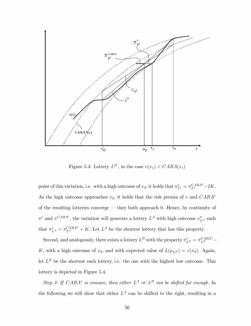
xx4x3LLBx’LLB

CARA*(x)

v(x)

vLLB­

CARALLB

*

LB

CLLB

µ

Figure 5.4: Lottery LB , in the case v(x1) < CARA(x1)

point of this variation, i.e. with a high outcome of x3, it holds that �vL� = �CARA�L� �2K.

As the high outcome approaches x2, it holds that the risk premia of v and CARA�

of the resulting lotteries converge � they both approach 0. Hence, by continuity of

�v and �CARA�, the variation will generate a lottery LA with high outcome x00LA such

that �vLA = �CARA�

LA +K. Let LA be the shortest lottery that has this property.

Second, and analogously, there exists a lottery LB with the property �vLB = �CARA�

LB �

K, with a high outcome of x4, and with expected value of L(�LB) = v(x3). Again,

let LB be the shortest such lottery, i.e. the one with the highest low outcome. This

lottery is depicted in Figure 5.4.

Step 3: If CARA� is concave, then either LA or LB can be shifted far enough. In

the following we will show that either LA can be shifted to the right, resulting in a

56

lottery L eA with expected utility L eA(�L eA) = v(x3) or LB can be shifted to the left,

resulting in a lottery L eB with expected utility L eB(�L eB) = v(x2). By the observationsin the previous step, this su¢ ces to prove the result (for the case that CARA� is

concave). We consider 4 cases � two with v(x1) < CARA�(x1) (as in Figures 5.3

and 5.4), and two with v(x1) > CARA�(x1).

Case 1: v(x1) < CARA�(x1), and LA is longer than LB, i.e. x00LA � x1 > x4 � x0LB .

First notice that the line HLA lies above the lottery line of LA. (See Figure 5.3: HLA

is a straight line through (x1; v(x1)) and (x00LA ; CARA�(x00LA +K)) � it is not drawn

in the �gure, to avoid having too many lines.) Hence, the value x�HA, where HLA

intersects CLA, lies to the left of �LA, i.e. x�HA � �LA. Similarly, for lottery L

B,

consider the auxiliary straight line HLB through (x4; v(x4)) and (x0LB ; CARA�(x0LB �

K)). HLB lies below CLB , so it holds that �LB � x�HB .

Now shift LB to the left, such that the low outcome of the resulting lottery LB0

is equal to x1 � which is clearly possible without leaving [x; x]. Let x00LB

0 be the

high outcome of LB0, and �LB0 be its expected value. We will show that for this

shifted lottery we have LB0(�LB0 ) � v(x2), which implies the desired result, because

by continuity of v there must then exist another shifted version of LB, L eB, withLeB(�L eB) = v(x2).For the shifted lottery LB

0, consider the auxiliary lines HLB0 and CLB0 , which in-

tersect at a point x�HB0 . Due to property (iii) of the lemma, the relative x-location of

this intersection is constant, i.e. it holds that x�HB0 = x

00LB

0� (x4�x�HB). This implies

that �LB0 � x�HB0 , because both xLB0 and x

�HB0 were shifted by the same 4x (from

x�LB and x�HB).

It holds that CLA(�LA) = v(x2) by construction. x�HA � �LA then implies that

CLA(x�HA) � v(x2), because CLA is increasing. From property (iv) of the lemma, it

57

holds that CLB0 (x�HB0 ) < CLA(x

�HA): LA is longer than LB

0and both have the same

low outcome x1, so the property applies here.

From above, we know that �LB0 � x�HB0 . But for all values x � x�HB0 it holds that

HLB0 (x) � CLB0 (x�HB0 ), becauseHLB0 andCLB0 intersect in x�HB0 . Hence,HLB0 (�LB0 ) �

CLB0 (x�HB0 ), and since the lottery line L

B0 lies below HLB0 , it holds that LB0(�LB0 ) �

HLB0 (�LB0 ). Collecting the above inequalities, it holds that LB0(�LB0 ) < v(x2).

Case 2: v(x1) < CARA�(x1), and LA is shorter than LB, i.e. x00LA � x1 � x4� x0LB :

Now shift lottery LA to the right, resulting in a lottery LA0with high outcome x4 and

expected value �LA0 . Construct the auxiliary lines HLA0 and CLA0 , which intersect at

x�HA0 . Analogous to the arguments in Case 1, it holds that x

�HA0 � �LA0 and x�HB �

�LB . Also analogous to the above arguments, one can show that CLB(x�HB) � v(x3),

CLA0 (x�HA0 ) � CLB(x

�HB), HLA0 (�LA0 ) � CLA0 (x

�HA0 ), and L

A0(x�LA

0 ) � HLA0 (�LA0 ).27

Hence, LA0(�LA0 ) � v(x3), and it follows that there exists a lottery L

eA with L eA(�L eA) =v(x3).

Case 3: CARA�(x1) < v(x1), and LA is shorter than LB, i.e. x00LA � x1 � x4� x0LB :

Again, shift LA to the right, resulting in a lottery LA0with high outcome x4 and

expected value �LA0 . Consider Figure 5.5, which depicts the auxiliary lines CLA0 and

CLB . Since both lotteries LB and LA0have the same high outcome, CLA0 lies above

CLB . As in Case 2, we will argue that LA0(�LA0 ) � v(x3). To this end, we �rst ask

where the lottery line LA0lies, relative to CLA0 . Observe that if the entire line L

A0 lies

27The following repeats the arguments, for this case. It holds that CLB (�LB ) = v(x3) by con-

struction. x�HB � �LB then implies that CLB (x�HB ) � v(x3), because CLB is increasing. Property

(iv) of the lemma yields CLB (x�HB ) � CLA0 (x�HA0 ): L

B is longer than LA0and both have the

same high outcome x4. From above, we know that x�HA0 � �LA0 , so that HLA0 (x) � CLA0 (x

�HA0 ).

Hence, HLA0 (�LA0 ) � CLA0 (x�HA0 ), and since the lottery line L

A0lies above HLA0 , it holds that

LA0(�LA0 ) � HLA0 (�LA0 ).

58

xx3 x4LLBx’LLA’x’LLB x~

v(x)

CLLB

CLLA’

LA’

µ

Figure 5.5: Location of CLB , CLA0 and LA0 in Case 3 of Step 3.

59

above v(x3), then we are done � LA0(�LA0 ) � v(x3) must be true in this case. Hence,

assume to the contrary that the low payo¤ of LA0lies below v(x3), LA

0(x0LA0) < v(x3),

as in the �gure. LA0crosses the horizontal line at level v(x3) somewhere, because its

high payo¤ is x4, and v is increasing. Furthermore, we will show in the next paragraph

that at v-level v(x3), LA0necessarily lies to the left of CLA0 . Otherwise, there would

exist a lottery bL that is shorter than LB but has all of the properties of LB: it wouldhold that �vbL = �CARA�bL +K, x00(bL) = x4, and bL(�bL) = v(x3). This would contradictthe de�nition of LB as the shortest lottery with these properties.

The following shows existence of bL, for this case. Consider the lottery bbL withoutcomes x0

LA0 and x4, and an expected value �bbL that is chosen such that bbL(�bbL) =

v(x3). If LA0lies to the right of CLA0 at v-level v(x3), then it follows that �

vbbL >�CARA

�bbL + K. Hence, we can increase the lower outcome of this lottery, keeping

the expected value �bbL constant, until (by continuity) there results a lottery bL with�vbL = �CARA�bL +K, as claimed in the previous paragraph.

The observation that LA0lies to the left of CLA0 at v-level v(x3) implies that there

exists a value ex where CLA0 crosses the horizontal line at level v(x3), see Figure 5.5.(This is true because otherwise CLA0 would lie entirely above the horizontal line at

v(x3) and could therefore not lie to the right of LA0at v(x3).) Also, it holds that LA

0

lies above CLA0 at ex, i.e. LA0(ex) � CLA0 (ex) = v(x3).Next, construct the auxiliary lines JLB and JLA0 , which intersect with CLB and

CLA0 , respectively, at x�JB and x

�JA

0 . Analogous to Case 1, it holds that x�JB � �LB

and x�JA0

� �LA0 . The �rst of these inequalities implies that CLB(x�JB) � CLB(�LB)

because CLB is increasing, and hence CLB(x�JB) � v(x3).

Now, we have

CLA0 (x�JA

0 ) � CLB(x�JB) � v(x3),

60

where the �rst inequality is implied by property (iv) of the lemma. Since CLA0 is

increasing and reaches the level v(x3) at ex, this implies that x�JA0 � ex. Since LA0is increasing and lies above CLA0 at ex, it follows that LA0(x�JA0 ) � LA

0(ex) � v(x3).

Finally, since x�JA0

� �LA0 (and LA0 is increasing) it follows that LA

0(�LA0 ) � v(x3),

the desired result.

Case 4: CARA�(x1) < v(x1), and LA is longer than LB, i.e. x00LA � x1 > x4 � x0LB .

This is analogous to Case 3. Shift LB to the left, so that the resulting lottery LB0has

the lower outcome x1. Then, analogous versions of all arguments for Case 3 apply,

yielding LB0(�LB0 ) � v(x2).28

Step 4: The previous steps show the result for the case that CARA� is concave.

This can be used to show that if CARA� is convex, the result holds as well.

Suppose that CARA� is convex. Consider the functions that describe v and

CARA�, from upside-down: bv = �v(�x) and \CARA�(x) = �CARA�(�x). Both of

these mirrored functions are increasing in x, on the interval [�x;�x], and \CARA�

is concave. Also, for any CARA function CARA : x ! CARA(x), it holds that

\CARA : x ! �CARA(�x) is also a CARA function, and that the horizontal dis-

tance between v and CARA on [x; x] is equal to the horizontal distance between bv and28The following sketches the steps: CLB0 lies above CLA . If the entire line L

B0lies below v(x2),

then LB0(�LB0 ) � v(x2) holds. Assume to the contrary that LB

0(x00LB0) > v(x2). LB

0crosses the

horizontal line at level v(x2) to the right of CLB0 , because otherwise the de�nition of LA would

be violated. Hence, there exists a value eex where CLB0 crosses the horizontal line at level v(x2),and LB

0(eex) � CLB0 (eex) = v(x2). For the locations where the auxiliary lines JLA and JLB0 intersect

with CLA and CLB0 , respectively, it holds that x�JA � �LA and x�JB0 � �LB0 . Therefore, and from

property (iv) of the lemma, we have CLB0 (x�JB0) � CLA(x�JA) � v(x2). Since CLB0 is increasing and

reaches v(x2) at eex, this implies that x�JB0 � eex. Since LB0is increasing and x�

JB0� �LB0 , it follows

that LB0(�LB0 ) � LB

0(x�JB0) � LB0

(eex) � v(x2).

61

\CARA on [�x;�x]. Hence, \CARA� is the best-�tting CARA function for bv on theinterval [�x;�x], with distance K (because if there were a CARA function CARA(�)

with a lower horizontal distance, then it would also be true that �CARA(�x) is a

CARA function with a lower horizontal distance from v on the interval [x; x]).

Hence, from the result of step 3, we know that there is a pair of shifted lotteries,

with payo¤s in [�x;�x], such that bv�s risk premium varies by at least K between

the two lotteries. This pair of lottery choice tasks can be re�ected around zero, by

reversing the sign of all payo¤s. Since bv is the mirror image of v, the resulting pair oflotteries has the property that v�s risk premium varies by at least K between the two

lotteries. Also, all payo¤s of the re�ected lotteries lie in [x; x]. Hence, we can apply

Proposition 1 to obtain the result. �

Lemma: Properties of CARA:

(For notation, see the �rst two paragraphs of the proof of Proposition 2.)

(i) Consider a set of three points f(x1; v1); (x2; v2); (x3; v3)g that is strictly monotonic:

x1 < x2 < x3 and v1 < v2 < v3. There exists a CARA function that connects the

three points.

(ii) For any CARA function CARA(�) and any binary lottery L, �CARAL is constant

across shifted versions of L, where 4x is added to both payo¤s as in Section 1. That

is, �CARAeL � �CARAL = 0.

(iii) Let (L; eL) be a pair of shifted lotteries. Then x�HeL � x0eL and x�JeL � x0eL are bothindependent of the shift 4x. That is, the relative location of x�HL and x

�JLdoes not

change if L is shifted.

(iv) Let �; r > 0, so that CARA is strictly concave. Consider a pair of lotteries

(eL; eeL) such that eeL that is longer than eL, i.e. x00eeL�x0eeL � x00eL�x0eL. If both eeL and eL havethe same low payo¤ (x0eeL = x0eL), then CL(x�HeeL) � CL(x

�HeL) and CL(x�JeeL) � CL(x

�JeL), i.e.

62

for the longer lottery, both values CL(x�HL) and CL(x�JL) are larger than for the shorter

lottery. If both have the same high payo¤ (x00eeL = x00eL), then the reverse inequalitiesare true, CL(x�HeeL) � CL(x

�HeL) and CL(x�JeeL) � CL(x

�JeL).

(v) Consider two CARA functionsCARA1(x) = �1��1 exp(�r1x) andCARA2(x) =

�2 � �2 exp(�r2x). Their horizontal distance �(x;CARA1; CARA2) is unimodal: its

derivative w.r.t. x changes its sign no more than once.

Proof: (i) For a CARA function with parameters �; �; r to connect (x1; v1) and

(x3; v3), we need

v1= � � � exp(�rx1)

v3= � � � exp(�rx3).

First restrict attention to the case that the CARA function is strictly concave (i.e.

�; r > 0) and that � > v3. Under these conditions, the above equations imply that �

can be expressed as a function of �,

�=exp(x3

x3 � x1ln(� � v1)�

x1x3 � x1

ln(� � v3))

=(� � v1)

x3x3�x1

(� � v3)x1

x3�x1.

Plugging the �rst of the expressions for � into the equation for v1 yields an expression

for r, as a function of �:

r =ln(� � v1)� ln(� � v3)

x3 � x1

Now vary �, and ask what values can the CARA function have at x2, if it connects

(x1; v1) and (x3; v3). Using the above expressions for � and r, it holds that

CARA(x2)= � � � exp(�rx2)

= � � (� � v1)x3�x2x3�x1 (� � v3)

x2�x1x3�x1 .

63

As � approaches v3 from above, this expression approaches v3. Also, as � approaches

1, r approaches 0, and therefore the function becomes approximately linear between

x1 and x3. Hence, by varying �, all points (x2; v2) that lie in the triangle between

(x1; v3), (x1; v1) and (x3; v3) can be reached by a concave CARA function that also

connects (x1; v1) and (x3; v3).

Now, consider the points that lie below the straight line between (x1; v1) and

(x3; v3). The upside-down images of convex CARA functions are concave CARA func-

tions (�CARA(�x), like in step 4 of the proof of Proposition 2), so that the above ar-

gument applies: we can �nd a convex CARA function connecting (x1; v1); (x2; v2); and

(x3; v3) i¤ we can �nd a concave CARA function connecting (�x3;�v3); (�x2;�v2);

and (�x1;�v1). This can be achieved by the above construction.

(ii) For a binary lottery L with lower payo¤ x0L, express the higher payo¤ as x00L =

x0L + �00 and the expected value as �L = x0L +

b�. By the de�nition of the certaintyequivalent CECARAL ,

CARA(CECARAL )=Pr(x0L)CARA(x0L) + (1� Pr(x0L))CARA(x00L)

=�00 � b��00

CARA(x0L) +b��00CARA(x0L + �

00).

Using the functional form of CARA, and �CARAL = �L � CECARAL , this is equivalent

to

exp(�r(b� � �CARAL )) =�00 � b��00

+b��00exp(�r�00),

which implicitly de�nes �CARAL independent of the lottery�s lower payo¤ x0L. Since

shifting the lottery to eL is equivalent to a shift in x0L while keeping �00 and b� constant,it follows that �CARAL = �CARAeL .

(iii) It is straightforward to check that the relative location of x�HL is

x�HL � x0L

x00L � x0L=

eKr

e�r(x00L�x0L) + eKr

.

64

Since 4x is added to both x00L and x0L, the term (x00L�x0L) is constant. Hence,x�HL

�x0Lx00L�x0L

is constant.

Similarly, one can check that x�JL has the relative location

x�JL � x0L

x00L � x0L= � (1� e�rK)

(e�rK � 1� erK�r(x00L�x0L) + e�r(x00L�x0L)).

This expression, too, depends only on (x00L � x0L), so it is constant across shifts of the

lottery.

(iv) To calculate CL(x�HL), �rst solvex�HL

�x0Lx00L�x0L

= eKr

e�r(x00

L�x0

L)+eKr

for x�HL :

x�HL =1

e�r(x00L�x0L) + eKr

�x0Le

�r(x00L�x0L) + x00LeKr�

The functional form of CL is given by

CL(x) = � � (� exp(�rx0L))(1 +x� x0Lx00L � x0L

(exp(�r(x00L � x0L))� 1)).

Plugging x�HL into this expression yields

CL(x�HL) = � � � e

Kr�rx00L + e�rx00L

e�r(x00L�x0L) + eKr

.

Taking partial derivatives, one can see that the expression is increasing in both vari-

ables x0L and x00L, if � > 0 and r > 0. Now, observe that if eeL is longer than eL and

the two lotteries have the same lower payo¤, then eeL can be generated from eL byincreasing x00eL, so the inequality CL(x�HeeL) � CL(x

�HeL) follows from the monotonicity

of CL(x�HL) in x00L. If they have the same higher payo¤, then

eeL can be generated fromeL by decreasing x0eL, and CL(x�HeeL) � CL(x

�HeL) follows from the monotonicity in x0L.

Similarly, one can check that the intersection of CL and JL occurs at v-level

CL(x�JL) = � � �e�rx0L + �e�rK e�rx

0L � e�rx00L

e�rK + e�r(x00L�x0L)

,

65

and again, the partial derivatives with respect to x0L and x00L show that the expression

is increasing in both x0L and x00L, if � > 0 and r > 0. The same reasoning as in the

previous paragraph then yields the results for CL(x�JeeL) and CL(x�JeL).

(v) The horizontal distance betweenCARA1 andCARA2 is given by �(x;CARA1; CARA2) =

x�CARA�12 (CARA1(x)). The inverse of CARA2 is given byCARA�12 (v) = � 1r2ln(�2�v

�2).

Hence, �(x;CARA1; CARA2) = x+ 1r2ln(�2��1+�1 exp(�r1x)

�2).

The statement is true because the second derivative of � w.r.t. x is

d2

dx2�(x;CARA1; CARA2) =

(�2 � �1)(�r1)2�1 exp(�r1x)((�2 � �1)�1 exp(�r1x))2

,

which has a constant sign. �

Proof of Proposition 3. We show a more general version of the proposition,

which covers the case that choices are representable by maximizing over m the ex-

pression

U(m) =

Zu(xI)dF (xI jm) +

Xi

Zv(xi)dLi(xijmi).

Here, u is the global evaluation of the distribution of total earnings, and v is the local

or narrow evaluation of wealth changes in each bracket. Both are assumed to be in-

creasing and twice continuously di¤erentiable. This generalizes the assumptions made

in Section 1, where v(x) = (1 � �)u(x). In the following version of the proposition,

there are only two choices to be made (I = 2) but this is only a simpli�cation. As we

will see, the gambles o¤ered in brackets 1 and 2 (to be constructed in the proof) can

be made arbitrarily small for the result to hold, so that by the continuity of u and v

these gambles would generally not a¤ect the choices in any other existing brackets,

unless these choices were knife-edge cases. Hence, �xing I = 2 is not restrictive �

for larger I, we can construct the I � 2 other choices to be non-knife-edge.

Proposition 30: Let u and v be strictly increasing and twice continuously

66

di¤erentiable, and suppose that v is not a member of the CARA family

of functions. Then there is a pair of binary choices, each between a 50/50

lottery and a sure payment, where a decisionmaker who maximizes U(�)

violates FOSD.

Proof: We will show that there exists a pair of 50/50 lottery choices of the following

kind, violating FOSD:

Reject gamble 1: A 50/50 gamble between x1�y1 and x1+z, with y1; z > 0, versus

x1 for sure.

Accept gamble 2: A 50/50 gamble between x2�y2 and x2+z, with y2; z > 0, versus

x1 for sure. Importantly, y2 > y1.

Due to y2 > y1, the choice combination (reject1; accept2) is FOS-dominated by

(reject2; accept1). We �nd appropriate values of x1; x2; y1; y2; z in two steps.

(i) If v is di¤erentiable but not CARA, then there exist payo¤s x�1 6= x�2 such that the

Arrow-Pratt degree of risk aversion rAP (x) = �v00(x)v0(x) is di¤erent at the two locations.

This can be shown by showing the reverse statement: suppose that rAP (x) is constant

and equal to some value r, at all x. Then we have a �rst-order linear di¤erential

equation for the function v0: v00(x) + rv0(x) = 0, which has the general solution

v0(x) = � exp(�rx). Integrating yields the general solution v(x) = � � � exp(�rx),

i.e. that v is CARA.

(ii) Consider a fair 50/50 gamble in an arbitrary bracket i: the decisionmaker can

either receive a certain payo¤xi or a 50/50 gamble between xi+� and xi��. (We will

show that as � gets small, the expression v00(x)v0(x) will be important, and that we would

need di¤erent certainty equivalents to o¤set the gamble at x�1 and x�2.) Fix the choices

in the other bracket at m�i, which will generate a distribution L�i(�jm�i) over the

sum of earnings in bracket �i. For any m�i, there exists a payment ci(xi; �;m�i) that

67

would need to be added to xi in order to make xi+ ci into a certainty equivalent, i.e.

for the decisionmaker to be indi¤erent between accepting and rejecting the gamble.

This payment ci(xi; �;m�i) is implicitly de�ned by U(x+ci(xi; �;m�i)jrejecti;m�i) =

U(xjaccepti;m�i). Using the global-plus-local form, this isZu(x+ xi + ci(xi; �;m�i))dL�i(xjm�i) + v(xi + ci(xi; �;m�i))

�Z1

2[u(x+ xi + �) + u(x+ xi � �)]dL�i(xjm�i)�

1

2[v(xi + �) + v(xi � �)]

= 0.

With �x xi and m�i, we can view this as h(�; ci(�)) = 0, and apply the implicit

function theorem to �nd that

dcid�=� (@h=@�)

(@h=@ci)

=

R12u0(x+ xi + �)� 1

2u0(x+ xi � �)dL�i(xjm�i) +

12[v0(xi + �)� v0(xi � �)]R

u0(x+ xi + ci(�))dL�i(xjm�i) + v0(xi + ci(�)).

Now consider the pair of brackets labeled 1 and 2, and simultaneously o¤er such a

50/50 gamble to win or lose � in both of them, starting from sure payo¤s of x�1 and x�2

(taken from part (i) above). Now, since the decisionmaker can either accept or reject

the gamble in the other bracket j (with j 2 f1; 2g and j 6= i), we have to consider two

cases for m�i in the expression for dcid�. But di¤erentiating both of these expressions

once again with respect to �, and taking the limit �! 0, it is straightforward to see

that for both possible choices mj 2 facceptj; rejectjg, the second derivative of ci(�)

has the same limit:

lim�!0

d

d�

dcid�(acceptj) = lim

�!0

d

d�

dcid�(rejectj) =

u00(x�i + x�j) + v

00(x�i )

u0(x�i + x�j) + v

0(x�i )

(The complete expressions for dd�(dcd�), evaluated separately at mj 2 facceptj; rejectjg,

are available upon request.)

68

Now compare this expression between i = 1 and i = 2. In the denominator and

in the numerator, respectively, the same expressions u00(x�i + x�j) and u

0(x�i + x�j) are

added in both brackets. But v00(x�1)v0(x�1)

6= v00(x�2)v0(x�2)

by the result of (i). Hence, there is

an � such that the second derivative of ci(xi; �;m�i) is di¤erent between i = 1 and

i = 2, for all � < �. This holds irrespective of the behavior in bracket j 6= i, because

the limit of dd�dcid�is the same for both possible values of mj. That is, even if the

choice in bracket j changes arbitrarily often as � approaches 0, it is still true that

dd�dcid�approaches a di¤erent limit in the two brackets. Hence, there is an � < � such

that the certainty equivalent itself is di¤erent, i.e. c1(x�1; �) 6= c2(x�2; �), because if

two functions have di¤erent continuous second derivatives over an interval, then they

have a di¤erent value somewhere in that interval. W.l.o.g., assume c(x�1; �) < c(x�2; �).

Then, by the de�nition of a certainty equivalent and by monotonicity of u and v,

there exists a value c with c(x�1; �) < c < c(x�2; �), such that the decisionmaker strictly

prefers to get x�1 + c for sure over the 50/50 gamble between x�1 + � and x

�1 � �, and

he strictly prefers the 50/50 gamble between x�2 + � and x�2 � � over x�2 + c for sure.

Hence, the desired payo¤s exist: pick a � that is small enough to not change these

choices, and set x1 = x�1 + c; x2 = x�2 + c; y1 = �+ c; y2 = �+ c+ �; z = �� c. �

69